Evolutionary Optimization of Least-Squares Support Vector ... · Evolutionary Optimization of Least-Squares Support Vector Machines 3 2 Kernel Machines All Kernel Machines rely on

Evolutionary Optimization of Least-SquaresSupport Vector Machines

Arjan Gijsberts, Giorgio Metta and Leon Rothkrantz

Abstract The performance of Kernel Machines depends to a large extent on its ker-nel function and hyperparameters. Selecting these is traditionally done using intu-ition or a costly “trial-and-error” approach, which typically prevents these methodsfrom being used to their fullest extent. Therefore, two automated approaches arepresented for the selection of a suitable kernel function and optimal hyperparam-eters for the Least-Squares Support Vector Machine. The first approach uses Evo-lution Strategies, Genetic Algorithms, and Genetic Algorithms with floating pointrepresentation to find optimal hyperparameters in a timely manner. On benchmarkdata sets the standard Genetic Algorithms approach outperforms the two other evo-lutionary algorithms and is shown to be more efficient than grid search. The sec-ond approach aims to improve the generalization capacity of the machine by evolv-ing combined kernel functions using Genetic Programming. Empirical studies showthat this model indeed increases the generalization performance of the machine, al-though this improvement comes at a high computational cost. This suggests that theapproach may be justified primarily in applications where prediction errors can havesevere consequences, such as in medical settings.

Arjan GijsbertsItalian Institute of Technology, Via Morego, 30 – Genoa 16163, ItalyDelft University of Technology, Mekelweg 4, 2628 CD Delft, The Netherlandse-mail: [email protected]

Giorgio MettaItalian Institute of Technology, Via Morego, 30 – Genoa 16163, ItalyUniversity of Genoa, Viale F. Causa, 13 – Genoa 16145, Italye-mail: [email protected]

Leon RothkrantzDelft University of Technology, Mekelweg 4, 2628 CD Delft, The NetherlandsNetherlands Defence Academy, Nieuwe Diep 8, 1781 AT Den Helder, The Netherlandse-mail: [email protected]

1

2 Arjan Gijsberts, Giorgio Metta and Leon Rothkrantz

1 Introduction

Kernel Machines allow the construction of powerful, non-linear classifiers using rel-atively simple mathematical and computational techniques [35]. As such, they havesuccessfully been applied in fields as diverse as data mining, economics, biology,medicine, and robotics. Much of the success of the Kernel Machines is due to thekernel trick, which can best be described as an implicit mapping of the input datainto a high dimensional feature space. In this manner, the algorithms can be appliedin a high dimensional space, without the need to explicitly map the data points. Thisimplicit mapping is done by means of a kernel function, which represents the innerproduct for the specific hypothetical feature space.

The performance of Kernel Machines is highly dependent on the chosen ker-nel function and parameter settings. Unfortunately, there are no analytical meth-ods or strong heuristics that can guide the user in selecting an appropriate kernelfunction and good parameter values. The common way of finding optimal hyperpa-rameters is to use a costly grid search, which scales exponentially with the numberof parameters. Additionally, it is usually necessary to manually determine the re-gion and resolution of the search to ensure computational feasibility. Selection ofthe kernel function is done similarly, i.e. either trial-and-error or only consideringthe default Gaussian kernel function. Consequently, tuning the techniques may bearduous, such that less than optimal performance is achieved. For a successful inte-gration in real-life information systems, Kernel Machines should be combined withan automated, efficient optimization strategy for both hyperparameters and kernelfunction.

Two distinct approaches are proposed for the automated selection of the param-eters and the kernel function itself. These models are based on techniques thatfall in the class of Evolutionary Computation, which are techniques inspired byneo-Darwinian evolution. The first approach uses evolutionary algorithms to op-timize the hyperparameters of a Kernel Machine in a time-efficient manner. Thesecond aims to increase the generalization performance by constructing combined,problem-specific kernel functions using Genetic Programming. Implementations ofboth approaches have been evaluated on seven benchmark data sets, for which tra-ditional grid search was used as a reference.

Kernel Machines and the kernel trick are presented in Sect. 2. We emphasize onone particular type of Kernel Machine, namely the Least-Squares Support VectorMachine. In Sect. 3, an introduction is given into the evolutionary algorithms thatare used in the models. A review of related work on hyperparameter optimizationand kernel construction is given in Sect. 4. The two approaches are presented inSect. 5, after which the experimental results are presented in Sect. 6. The paper isfinalized in Sect. 7 with the conclusions and suggestions for future work.

Evolutionary Optimization of Least-Squares Support Vector Machines 3

2 Kernel Machines

All Kernel Machines rely on a kernel function to transform a non-linear probleminto a linear one by mapping the input data into a hypothetical, high dimensionalfeature space. This mapping – the kernel trick – is not done explicitly, as the kernelfunction calculates the inner product in the corresponding feature space. The kerneltrick is explained together with the Least-Squares Support Vector Machine (LS-SVM), which is a particular type of Kernel Machine.

2.1 Least-Squares Support Vector Machines

Assume a set of ` labeled training samples, i.e. S = {(xi,yi)}`i=1, where x∈X ⊆Rn

is an input vector of n features and y ∈ Y is the corresponding label. In the case Ydenotes a set of discrete classes, e.g. Y ⊆ {−1,1}, then the problem is considered aclassification problem. Conversely, if Y ⊆R, then we are dealing with a regressionproblem. The LS-SVM aims to construct a linear function [37]

f (x) = 〈x,w〉+ b , (1)

which is able to predict an output value y given an input sample x. Note that forbinary classification purposes it is necessary to apply the sign function on the pre-dicted output value. The error in the prediction for each sample i is defined as

yi− (〈xi,w〉+ b) = εi for 1≤ i≤ ` . (2)

The optimization problem in LS-SVM is analogous to that of traditional SupportVector Machines (SVM) [38]. The goal is to minimize both the norm of the weightvector w (i.e. maximize the margin) and the sum of the squared errors. In contrastto SVM, LS-SVM uses equality constraints for the errors instead of inequality con-straints. Combining the optimization problem with the equality constraints for theerrors (2), one obtains

minimize12‖w‖2 +

12

C`

∑i=1

ε2i (3)

subject to yi = 〈xi,w〉+ b + εi for 1≤ i≤ ` ,

where C is the regularization parameter. Reformulating this optimization problemas a Lagrangian gives the unconstrained minimization problem

12‖w‖2 +

12

C`

∑i=1

ε2i −

`

∑i=1

αi (〈xi,w〉+ b + εi− yi) , (4)

where αi ∈ R for 1 ≤ i ≤ `. Note that the Lagrange multipliers αi can be eitherpositive or negative, due to the equality constraints in the LS-SVM algorithm. The


optimality conditions for this problem can be obtained by setting all derivativesequal to zero. This yields a set of linear equations

`

∑j=1

α j⟨x j,xi

⟩+ b +C−1

αi = yi for 1≤ i≤ ` . (5)

2.2 Kernel Functions

We observe that the training samples are only present within the inner products in(5). The kernel function used to compute an inner product is defined as

k (x,z) = 〈φ (x) ,φ (z)〉 , (6)

where φ (x) is the mapping of the input samples into a feature space. If we substitutethe standard inner product with a kernel function in (5), we obtain the “kernelized”variant

`

∑j=1

α jk (x j,xi)+ b +C−1αi = yi for 1≤ i≤ ` . (7)

Usually it is convenient to define a symmetric kernel matrix as K = (k (xi,x j))`i, j=1,

so that the system of linear equations can be rewritten as[K +C−1I 1

1T 0

][α

b

]=[

y0

]. (8)

Note that the bottom row and rightmost column have been added to integrate thebias b in the system of linear equations. Other than the sign function, the algorithmis identical for both regression and classification. After the optimal Lagrange multi-pliers and bias have been obtained using (8), unseen samples can be predicted using

f (x) =`

∑i=1

αik (xi,x)+ b . (9)

2.2.1 Conditions for Kernels

It is important to obtain functions that correspond to an inner product in some fea-ture space. Mercer’s theorem states that valid kernel functions must be symmetric,continuous, and positive semi-definite [38], formalized as the following condition:∫

X ×Xk (x,z) f (x) f (z)dxdz≥ 0 for all f ∈ L2 (X ) . (10)


Kernel functions that satisfy these conditions are referred to as admissible kernelfunctions. If this condition is satisfied, then the kernel matrix is accordingly posi-tive semi-definite [4]. Unfortunately, it is not trivial to verify that a kernel functionsatisfies Mercer’s condition, nor whether the kernel matrix is positive semi-definite.There are, however, certain functions that have analytically been proven to be ad-missible. Common kernel functions – for classification and regression purposes –include the polynomial (11), the RBF (12), and the sigmoid function (13). Note thatthe sigmoid kernel function is only admissible for certain parameter values.

k (x,z) =(〈x,z〉+ c)d for d ∈ N, c≥ 0 (11)

k (x,z) =exp(−γ‖x− z‖2) for γ > 0 (12)

k (x,z) = tanh(γ 〈x,z〉+ c) for some γ > 0,c ≥ 0 (13)

All these function are parameterized, allowing for adjustments with respect tothe training data. The kernel parameter(s) and the regularization parameter C are thehyperparameters. The performance of an LS-SVM (or an SVM, for that matter) iscritically dependent on the selection of hyperparameters.

Mercer’s condition can be used to infer simple operations for creating combinedkernel functions, which are also admissible. For instance, assume that k1 and k2are admissible kernel functions, then the following combined kernels are admissible[35]:

k (x,z) = c1k1 (x,z)+ c2k2 (x,z) for c1,c2 ≥ 0 (14)k (x,z) = k1 (x,z)k2 (x,z) (15)k (x,z) = ak2 (x,z) for a≥ 0 (16)

Moreover, these operations allow modular construction of kernel functions. In-creasingly complex kernel functions can be constructed by recursively applyingthese operations.

3 Evolutionary Computation

Several biologically inspired techniques have been developed over the years forsearch, optimization, and machine learning under the collective term Evolution-ary Computation (EC) [40]. The key principle in EC is that potential solutions aregenerated, evaluated, and reproduced iteratively. Between iterations, individuals aresubject to certain forms of mutation and can reproduce with a probability that is pro-portional to their fitness. A selection procedure removes individuals with low fitnessfrom the population, so that the more fit ones are more likely to “survive”. Threeof the main branches within EC are Genetic Algorithms, Evolution Strategies, andGenetic Programming.


3.1 Genetic Algorithms

Probably the most recognized form of EC is the class of Genetic Algorithms (GA),popularized by Holland [15]. Genetic Algorithms mainly operate in the realm ofthe genotype, which is commonly represented as a bitstring. This means that allparameters need to be converted to a binary representation and are then concatenatedto form the chromosome. Various types of bit encoding may be used, such as Graycodes or even floating point representations.

Reproduction of individuals is usually emphasized in preference to mutation inGA. Two or more parents exchange part of their chromosome, resulting in offspringthat contains genetic information from each of the parents. The common imple-mentation is crossover recombination, in which two parents exchange a fragment oftheir chromosome. The size of the fragment is determined by a randomly selectedcrossover point. Mutation, on the other hand, is implemented by flipping the bits inthe chromosome with a certain probability. Note that the implementation of both re-production and mutation operators may depend on the specific representation that isused. For instance, reproduction of floating point chromosomes is done by blendingthe parents [10].

In addition to the mutation and recombination operators, the other key element inGA is the selection mechanism. The selection procedure selects the individuals thatwill be subject to mutation and reproduction with a probability proportional to theirfitness. Further, offspring can be created on a generational interval or, alternatively,individuals can be replaced one by one (i.e. steady state GA).

3.2 Evolution Strategies

Evolution Strategies (ES) operate in the realm of the phenotype and use real-valuedrepresentations for the individuals [2]. An optimization problem with three param-eters is represented as a vector c = (x1,x2,x3), where the parameters xi ∈ R are theobject parameters. There are two main types of ES, namely (µ + λ )-ES and (µ,λ )-ES. In these notations, µ is the size of the parent population and λ is the size of theoffspring population. In (µ + λ )-ES, the new parent population is chosen from boththe current parent population and the offspring. In contrast, in (µ,λ )-ES the newparent population is chosen only from the offspring population, which requires thatλ ≥ µ .

The canonical ES relies solely on the mutation operation for diversifying thegenetic material. The mutation operation is typically implemented as a random per-turbation of the parameters according to a probability distribution. More formally,

x′i = xi +Ni (0,σi) , (17)

where N denotes a logarithmic normal distribution. Note that this mutation mech-anism requires the user to specify a standard deviation σi (i.e. the strategy parame-


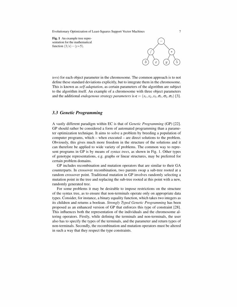
Fig. 1 An example tree repre-sentation for the mathematicalfunction (3/x)− (y∗5).

3 x

/

y 5

∗

−

ters) for each object parameter in the chromosome. The common approach is to notdefine these standard deviations explicitly, but to integrate them in the chromosome.This is known as self adaptation, as certain parameters of the algorithm are subjectto the algorithm itself. An example of a chromosome with three object parametersand the additional endogenous strategy parameters is c = (x1,x2,x3,σ1,σ2,σ3) [3].

3.3 Genetic Programming

A vastly different paradigm within EC is that of Genetic Programming (GP) [22].GP should rather be considered a form of automated programming than a parame-ter optimization technique. It aims to solve a problem by breeding a population ofcomputer programs, which – when executed – are direct solutions to the problem.Obviously, this gives much more freedom in the structure of the solutions and itcan therefore be applied to wide variety of problems. The common way to repre-sent programs in GP is by means of syntax trees, as shown in Fig. 1. Other typesof genotype representations, e.g. graphs or linear structures, may be preferred forcertain problem domains.

GP includes recombination and mutation operators that are similar to their GAcounterparts. In crossover recombination, two parents swap a sub-tree rooted at arandom crossover point. Traditional mutation in GP involves randomly selecting amutation point in the tree and replacing the sub-tree rooted at this point with a new,randomly generated tree.

For some problems it may be desirable to impose restrictions on the structureof the syntax tree, as to ensure that non-terminals operate only on appropriate datatypes. Consider, for instance, a binary equality function, which takes two integers asits children and returns a boolean. Strongly Typed Genetic Programming has beenproposed as an enhanced version of GP that enforces this type of constraint [28].This influences both the representation of the individuals and the chromosome al-tering operators. Firstly, while defining the terminals and non-terminals, the useralso has to specify the types of the terminals, and the parameter and return types ofnon-terminals. Secondly, the recombination and mutation operators must be alteredin such a way that they respect the type constraints.


4 Related Work

Hyperparameters and the kernel function are usually selected using a trial-and-errorapproach. Trial runs are performed using various configurations, the best of whichis selected. This approach is generally considered time consuming and does notscale well with the number of parameters. Furthermore, the process often yieldsless than optimal performance in situations where time is a limited. More elaborateapproaches have been suggested for both selection problems, which will be summa-rized below.

4.1 Hyperparameter Optimization

An analytical technique that has been proposed for hyperparameter optimization isthat of gradient descent [5, 20], which finds a local minimum by taking steps inthe negative gradient direction. This approach has been used for hyperparameterselection with a non-spherical RBF function, which means that each feature has adistinct scaling factor. Accordingly, there are more hyperparameters than there arefeatures, demonstrating the scalability of the approach. The gradient descent methodis shown to be able to find reasonable hyperparameters more efficiently than gridsearch. However, the method requires a continuous differentiable kernel and ob-jective function, which may not be satisfiable for specific types of problems (e.g.non-vectorial kernel functions). Approaches based on pattern search have been pro-posed to overcome this problem [27]. In this method the neighborhood of a parame-ter vector is investigated in order to approximate the gradient empirically. However,the whole class of gradient descent methods has the inherent disadvantage that theymay find local minima.

One of the first mentions of the use of EC for hyperparameter optimization canbe found in the work of Frohlich et al. [12], in which GA is primarily used for fea-ture selection. However, the optimization of the regularization parameter C is donein parallel. Other GA-based approaches focus mainly on the optimization of the hy-perparameters. The objective function in these type of approaches is either the erroron a validation set [18, 26, 29], the radius-margin bound [7], or k-fold cross valida-tion [6,33]. Some studies make use of a real-valued variant of GA [17,42], althoughit is not clear whether the real-valued representation performs significantly betterthan a binary representation. All these studies suggest that GA can successfully beapplied for hyperparameter optimization. However, there are some caveats, such asheterogeneity of the solutions and the selection of a reliable and efficient objectivefunction.

ES have only scarcely been used for hyperparameter optimization [11]. In thisapproach, ES optimizes not only the scaling, but also the orientation of the RBF ker-nel. An improvement on the generalization performance is achieved over the kernelparameters that were found using grid search. This result should be interpreted withcare, as the optimal grid search parameters are used as the initial solutions for the


evolutionary algorithm. The classification error on separate test sets is used as theempirical objective function.

The main advantage of evolutionary algorithms in comparison to grid searchis that they usually find good parameter settings efficiently and that the techniquescales well with the number of hyperparameters. An advantage compared to gradientdescent methods is that they cope better with local minima. Furthermore, they do notimpose requirements on the kernel and objective functions, such as differentiability.

4.2 Combined Kernel Functions

It is intuitive that combined kernel functions are capable of improving the gener-alization performance, as the implicit feature mapping can be tuned for a specificproblem. Several methods have been proposed for the composition of kernel func-tions. One of the first manifestations of combined kernel optimization was inves-tigated by Lanckriet et al. [23]. This work considers linear combinations of ker-nels, i.e. K = ∑

mi=0 aiKi for a > 0 and Ki chosen from a predefined set of kernel

functions. The optimization of weight factors a is done using semi-definite pro-gramming, which is an optimization method that deals with convex functions overthe convex cone of positive semi-definite matrices. This method can be applied tokernel matrices, since these need to be semi-definite to satisfy Mercer’s condition.However, other methods may be used for the optimization of the weights, such asso-called hyperkernels [30], the Lagrange multiplier method [19], or using a gener-alized eigenvalue approach [36].

Lee et al. argue that during the combination of kernels some potentially usefulinformation is lost [24]. They propose a method for combining kernels that aims toprevent this loss of information. Instead of combining various kernel matrices intoone, their method creates a large kernel matrix that contains all original kernel ma-trices and all possible mixtures of kernel functions, e.g. ki, j (x,z) =

⟨φi (x) ,φ j (z)

⟩,

where φi is the mapping that belongs to kernel function ki and φ j the mapping thatbelongs to kernel k j. This eliminates the requirement to optimize the weight factorfor each kernel, as this is done implicitly by the SVM algorithm. However, spe-cial mixture functions need to be provided for the combination of two kernel func-tions. Furthermore, the spatial and temporal requirements of the algorithm increasesdrastically, as the kernel matrix is enlarged in both dimensions in proportion to thenumber of kernels in the combination.

Other EC inspired approaches have been proposed to combine kernel functions.Most of these optimize a linear combination of weighted kernels using either GAor ES. The distinguishing elements are the set of kernel functions that is consid-ered and the type of combination operators. Some only consider linear combina-tions (i.e. the addition operator) [9, 31], whilst others may allow both addition andmultiplication [25]. These studies suggest that combining kernel functions can im-prove the generalization performance of the machine. However, the combinationsare restricted to a predefined size and structure.


Howley and Madden propose a method to construct complete kernel functionsusing GP [16]. In this method, a kernel function is evolved for use with an SVMclassifier. They use a tree structured genotype, with the operators +, −, and ×in both scalar and vector variants as the non-terminals. The terminals in their ap-proach are the two vectors x1 and x2. Since the kernels are constructed using sim-ple arithmetic, they are not guaranteed to satisfy Mercer’s condition. Nonetheless,the technique still keeps up with (or outperforms) traditional kernels for most datasets. It is emphasized that techniques such as GP require a sufficiently large dataset. Diosan et al. have proposed some enhancements; their method differs from theoriginal approach by an enriched operator set (e.g. various norms are included) andsmall changes to certain operators [8]. Similar modifications are presented for Ker-nel Nearest-Neighbor classification by Gagne et al., who also use co-evolution tokeep the approach computationally tractable [14]. Besides a species that evolveskernel functions, there are two other species for the training and validation sets. Thetraining set species cooperates with the kernel function on minimizing the error andthus maximizing the fitness, whereas the species for the validation set is competitiveand tries to maximize the error of the kernel functions.

5 Evolutionary Optimization of Kernel Machines

Two methods for the evolutionary optimization of hyperparameters and the ker-nel function are proposed. The first approach uses ES, GA, and GA with floatingpoint representation to optimize the hyperparameters for a given kernel function(EvoKMES, EvoKMGA, and EvoKMGAflt, respectively). The aim is to find optimalhyperparameters more efficiently than using traditional grid search. Our secondmodel uses GP to evolve combined kernel functions (EvoKMGP), with the aim toincrease the generalization performance.

5.1 Hyperparameter Optimization

In the hyperparameter optimization models, ES and GA are used to optimize thehyperparameters θ . Two variants of the GA model have been implemented; one thatuses the traditional bitstring representation with Gray coding and another that usesa floating point representation. Evolutionary algorithms are highly generalized andtheir application on this specific problem is straightforward.

In EvoKMES, the chromosomes contain the real-valued hyperparameters and thecorresponding endogenous strategy parameters σ , which yields for the RBF ker-nel the chromosome c =

[γ,C,σγ ,σC

]. Note that all the models use the hyper-

parameters on a logarithmic scale with base-2. Each hyperparameter is initializedto the center of its range and mutated according to the initial standard deviationσi = 1.0. An interesting issue is whether to use (µ + λ )-ES or (µ,λ )-ES in the


model. Both types have their own specific advantages and disadvantages. Typicalapplication areas of (µ + λ )-ES are discrete finite size search spaces, such as com-binatorial optimization problems [3]. When the problem is an unbounded, typicallyreal-valued search spaces, then (µ,λ )-ES is preferred [34]. Furthermore, Whitleypresents empirical evidence that indicates that (µ,λ )-ES generally performs betterthan (µ + λ )-ES [41]. We prefer to follow both the heuristic and the empirical indi-cations and adopted (µ,λ )-ES for our model. Unfortunately, there is no guaranteethat the search process will converge, as would have been the case with (µ + λ )-ES.For our model, we have empirically selected µ = 3 and λ = 12 based on preliminaryexperimentations.

EvoKMGA and EvoKMGAflt differ from EvoKMES in terms of the the operatorsand the genotype representation. EvoKMGA uses a Gray code of 18 bits for eachparameter, and one-point crossover recombination and bit-flip mutation operators.One disadvantage of GA, as compared to ES, is that there are many more parametersparameters that need to be set. The population size of 10 is relatively low for GAstandards. However, one must take into account that the maximum number of eval-uations is limited to several hundreds up to a few thousand and, moreover, the goalis to see convergence to good solutions within the first hundred evaluations. Largepopulation sizes, e.g. larger than 50, would have a disadvantage in this context, asthe algorithm can only perform one or two generations within this range. Further,preliminary experiments have shown that a population size of 10 shows similar con-vergence to larger population sizes. Other parameters of EvoKMGA have been tunedusing a coarse grid search as well. One-point crossover recombination occurs witha probability of pc = 0.2. During mutation, each bit in the chromosome is invertedwith a probability of pm = 0.1. The number of participants in tournament selectionis 5. Further, the steady state variant of GA has been used.

EvoKMGAflt, on the other hand, uses a floating point representation. Crossoverrecombination in this model is performed by blending two individuals using theBLX-α method [10]. This recombination operator is applied with a probabilityof pc = 0.3 and with α = 0.5. Additionally, each parameter has a probability ofpm = 0.4 of being mutated using a random perturbation according to the normaldistribution N (µ,σ), where µ = 0 and σ = 0.5. All other settings are equal tothose for EvoKMGA.

5.2 Kernel Construction

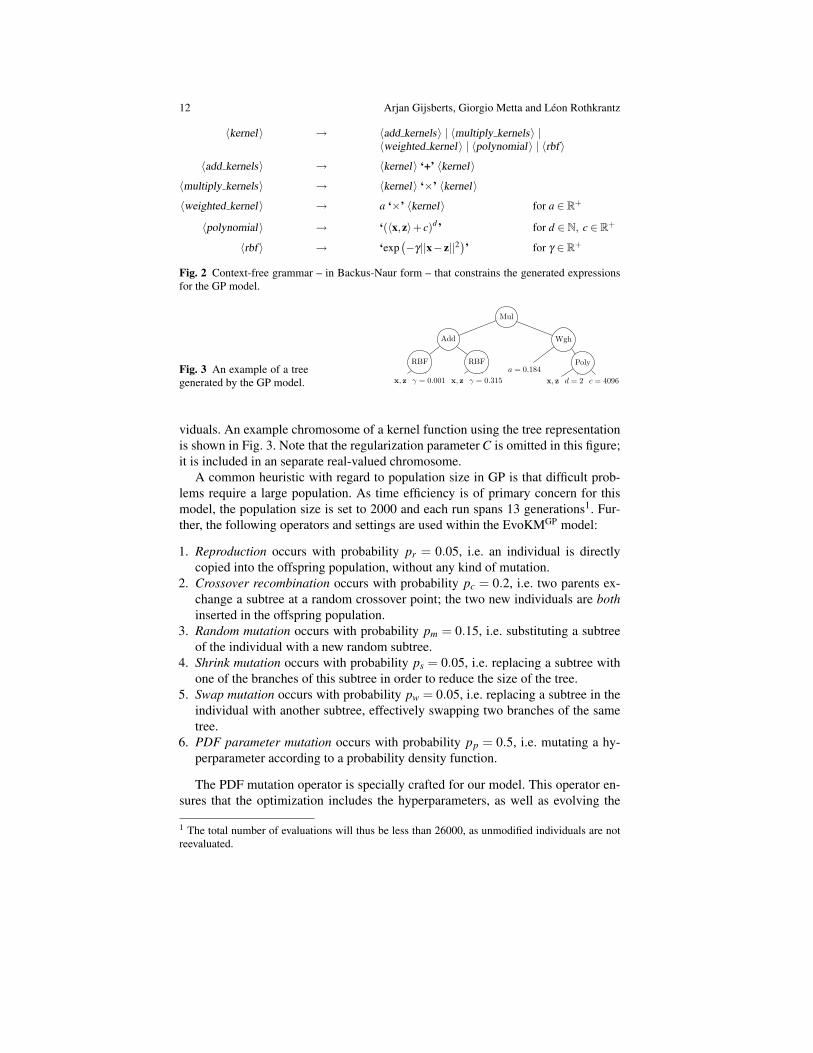
The second optimization method constructs complete kernel functions using GP. Inthis model, the functions are represented using syntax trees. The syntactic structureof the trees is based on the combination operations that guarantee admissible kernelfunctions, cf. (14), (15), and (16). These operations form the set of non-terminals,whereas the polynomial and RBF kernels form the set of terminals. This is formal-ized in the context-free grammar shown in Fig. 2. The model makes use of StronglyTyped GP, as it needs to ensure that the syntactic structure is enforced for all indi-


〈kernel〉 → 〈add kernels〉 | 〈multiply kernels〉 |〈weighted kernel〉 | 〈polynomial〉 | 〈rbf〉

〈add kernels〉 → 〈kernel〉 ‘+’ 〈kernel〉

〈multiply kernels〉 → 〈kernel〉 ‘×’ 〈kernel〉

〈weighted kernel〉 → a ‘×’ 〈kernel〉 for a ∈ R+

〈polynomial〉 → ‘(〈x,z〉+ c)d’ for d ∈ N, c ∈ R+

〈rbf〉 → ‘exp(−γ||x− z||2

)’ for γ ∈ R+

Fig. 2 Context-free grammar – in Backus-Naur form – that constrains the generated expressionsfor the GP model.

Fig. 3 An example of a treegenerated by the GP model. x, z γ = 0.001

RBF

x, z γ = 0.315

RBF

Add

a = 0.184x, z d = 2 c = 4096

Poly

Wgh

Mul

viduals. An example chromosome of a kernel function using the tree representationis shown in Fig. 3. Note that the regularization parameter C is omitted in this figure;it is included in an separate real-valued chromosome.

A common heuristic with regard to population size in GP is that difficult prob-lems require a large population. As time efficiency is of primary concern for thismodel, the population size is set to 2000 and each run spans 13 generations1. Fur-ther, the following operators and settings are used within the EvoKMGP model:

1. Reproduction occurs with probability pr = 0.05, i.e. an individual is directlycopied into the offspring population, without any kind of mutation.

2. Crossover recombination occurs with probability pc = 0.2, i.e. two parents ex-change a subtree at a random crossover point; the two new individuals are bothinserted in the offspring population.

3. Random mutation occurs with probability pm = 0.15, i.e. substituting a subtreeof the individual with a new random subtree.

4. Shrink mutation occurs with probability ps = 0.05, i.e. replacing a subtree withone of the branches of this subtree in order to reduce the size of the tree.

5. Swap mutation occurs with probability pw = 0.05, i.e. replacing a subtree in theindividual with another subtree, effectively swapping two branches of the sametree.

6. PDF parameter mutation occurs with probability pp = 0.5, i.e. mutating a hy-perparameter according to a probability density function.

The PDF mutation operator is specially crafted for our model. This operator en-sures that the optimization includes the hyperparameters, as well as evolving the

1 The total number of evaluations will thus be less than 26000, as unmodified individuals are notreevaluated.


structure of the kernel functions. The common GP operators would only be able tomutate these parameters by substituting them for another randomly selected param-eter.

5.3 Objective Function

When applying EC techniques it is important to decide which objective functionto use, as this is the actual measure that is being optimized. It should, therefore,measure the “quality” of a solution for the given domain. In the context of thisstudy quality is best described as the generalization performance of the machine.A very important aspect is that the fitness function must prevent overfitting of themachine to the training data. This is especially true for EvoKMGP, as this modeltunes both the hyperparameters and the kernel function for the specific data set.There are several methods to estimate this generalization performance, of whichcross validation can be applied to practically any learning method. Both k-fold andleave-one-out cross validation have been shown to be approximately unbiased interms of estimating the true expected error [21]. However, k-fold cross validationusually exhibits a lower variance on the error than the leave-one-out measure. Forthis reason, k-fold cross validation is used as fitness function for both approaches.

6 Results

All models have been validated experimentally on a standard set of benchmark prob-lems. An LS-SVM has been implemented in C++ using the efficient Atlas libraryfor Linear Algebra [39]. This implementation uses an approximate variant of theLS-SVM kernel machine [32], so as to reduce the computational demands of theexperiments. The size of the subset that is used to describe the model is set to 10%of the total data set. Although LS-SVM is only one specific type of kernel machine,all relevant aspects of the models have been kept generalized, so that extension toother types of Kernel Machines (e.g. SVM) is straightforward. Two kernel functionshave been considered in these experiments. The first is the RBF kernel function, cf.(12), which is commonly regarded the “default” choice for kernel machines. Thesecond is the polynomial function, cf. (11).

The evolutionary algorithms in the models have been implemented using theOpenBeagle framework for EC [13]. The objective function is, as explained, k-foldcross validation with k = 5. This value gives a adequate tradeoff between accuracyand computational expenses. For classification problems, the error measure is thenormalized classification error; in case of regression problems the mean-squared-error (MSE) is used.


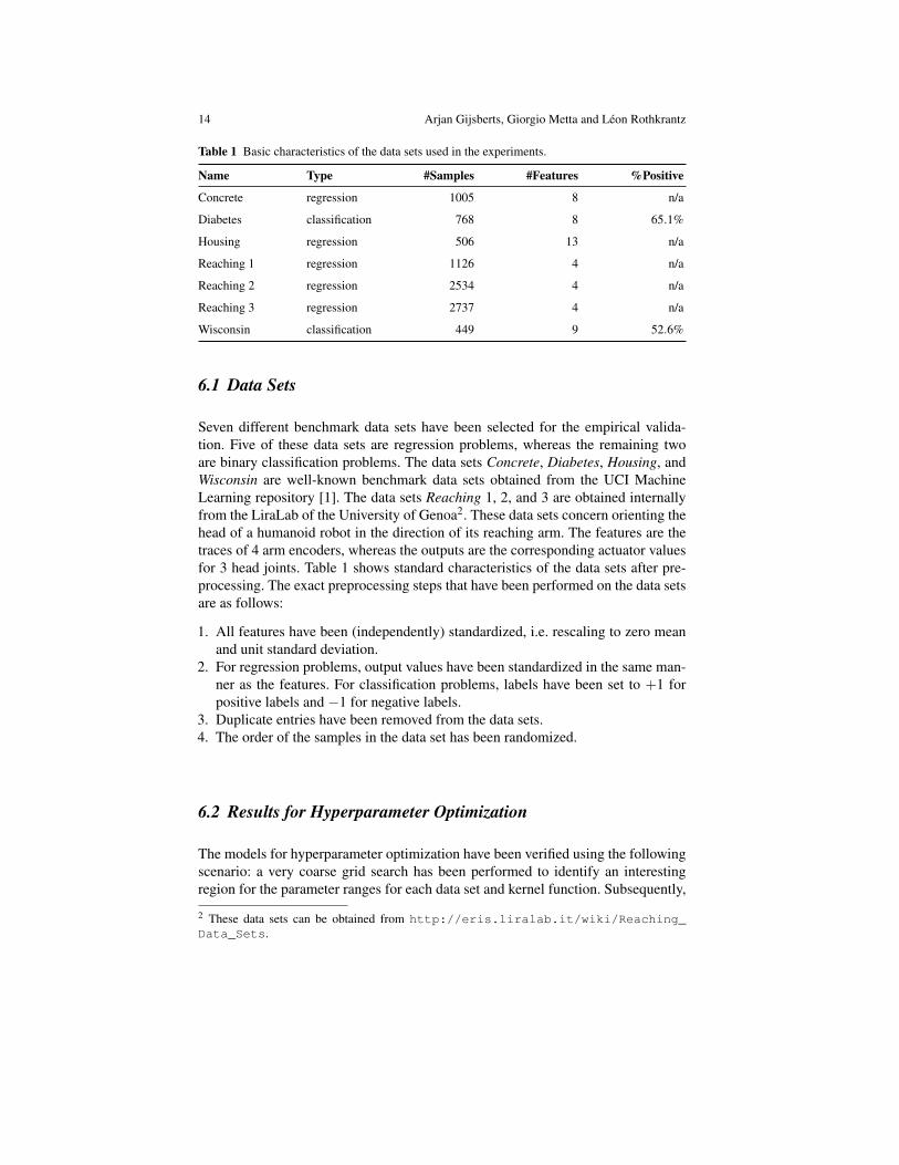
Table 1 Basic characteristics of the data sets used in the experiments.

Name Type #Samples #Features %Positive

Concrete regression 1005 8 n/a

Diabetes classification 768 8 65.1%

Housing regression 506 13 n/a

Reaching 1 regression 1126 4 n/a



Wisconsin classification 449 9 52.6%

6.1 Data Sets

Seven different benchmark data sets have been selected for the empirical valida-tion. Five of these data sets are regression problems, whereas the remaining twoare binary classification problems. The data sets Concrete, Diabetes, Housing, andWisconsin are well-known benchmark data sets obtained from the UCI MachineLearning repository [1]. The data sets Reaching 1, 2, and 3 are obtained internallyfrom the LiraLab of the University of Genoa2. These data sets concern orienting thehead of a humanoid robot in the direction of its reaching arm. The features are thetraces of 4 arm encoders, whereas the outputs are the corresponding actuator valuesfor 3 head joints. Table 1 shows standard characteristics of the data sets after pre-processing. The exact preprocessing steps that have been performed on the data setsare as follows:

1. All features have been (independently) standardized, i.e. rescaling to zero meanand unit standard deviation.

2. For regression problems, output values have been standardized in the same man-ner as the features. For classification problems, labels have been set to +1 forpositive labels and −1 for negative labels.

3. Duplicate entries have been removed from the data sets.4. The order of the samples in the data set has been randomized.

6.2 Results for Hyperparameter Optimization

The models for hyperparameter optimization have been verified using the followingscenario: a very coarse grid search has been performed to identify an interestingregion for the parameter ranges for each data set and kernel function. Subsequently,

2 These data sets can be obtained from http://eris.liralab.it/wiki/Reaching_Data_Sets.


a very dense grid search is performed on this region to establish a reference for ourmodels. For the polynomial kernel function, which has two parameters, the degreehas been kept fixed at d = 3 in order to keep the search computationally tractable.This reference contains the number of evaluations used for grid search3 and thecorresponding minimum error, which serves as the target for our models.

The evolutionary models have been used on the same parameter ranges as thegrid search. The only exception is that for the polynomial kernel we have not keptthe degree fixed at d = 3; instead it is set within a range of d = {1, ..,8}. Thisexception is made to investigate the scaling properties of the ES-based approach,i.e. to see whether evolutionary optimization can yield better solutions by optimizingmore parameters. The evolutionary search is terminated after the same number ofevaluations as used for the grid search.

A comparison of the generalization performance of the grid search and the evo-lutionary models is shown in Table 2. The overall impression is that all the evolu-tionary algorithms are able to find competitive solutions. In particular EvoKMGA

shows stable performance, as it finds equal or better solutions for all of the data sets.The only minor exception is the Diabetes data set, for which it finds solutions thatare only marginally worse than those found using grid search. Another observationis that for the majority of the data sets the inclusion of the degree of the polyno-mial kernel indeed decreases the generalization error. This suggests that the meth-ods scale well with the number of parameters and, moreover, that the extra degreeof freedom is used to decrease the error. Furthermore, EvoKMES and EvoKMGAflt

perform worse than that of the GA-based model on this real-valued optimizationproblem, suggesting that real-valued chromosomes are not necessarily beneficialfor hyperparameter optimization.

More interesting than the optimal solutions is the rate of convergence of the vari-ous methods. This has been analyzed by considering the number of evaluations thatwere needed to reach an error that is close to the target, cf. Table 3. These resultsconfirm the previous observation that EvoKMGA outperforms the two other modelsin most situations. The GA method converges to the target error in only a fraction ofthe number of evaluations used for grid search, with the exception of the Diabetesdata set. Furthermore, in almost all situations, it is able to find solutions within arange of 5% of the target within the first 100 evaluations.

The ES and GAflt methods converge slower than EvoKMGA, although EvoKMES

outperforms the others on a number of regression data sets. Conversely, it performsmuch worse on the Wisconsin classification data set. One of the reasons for thisbehavior is that ES uses the mutated offspring to sample the proximity of the parentindividuals. This information is then used to find a direction in which the error isdecreasing, in a manner similar to gradient descent or pattern search. The difficultywith classification problems is that the error surface incorporates plateaus. Offspringindividuals in the proximity of a parent are thus likely to have an identical fitnessscore and the algorithm will perform a random search on the plateau. Smoothnessof the fitness landscape may be regarded as a prerequisite to efficient optimization

3 Note that the number of evaluations directly translates into time, as solving the LS-SVM problemis independent of the chosen parameters.


Table 2 Comparison of the minimum errors of grid search and the evolutionary optimization meth-ods. Note that the results of the latter are averages over 25 runs.

Grid Search EvoKMES EvoKMGA EvoKMGAflt

Name Kernel εmin Eval. εmin εmin εmin

Concrete RBF 0.1607 1221 0.1591 ± 0.0000 0.1590 ± 0.0000 0.1590 ± 0.0000Poly. 0.1700 899 0.1741 ± 0.0000 0.1698 ± 0.0001 0.1778 ± 0.0235

Diabetes RBF 0.2200 621 0.2201 ± 0.0004 0.2202 ± 0.0006 0.2207 ± 0.0015Poly. 0.2213 777 0.2226 ± 0.0003 0.2215 ± 0.0012 0.2231 ± 0.0016

Housing RBF 0.1676 2793 0.1674 ± 0.0000 0.1674 ± 0.0000 0.1674 ± 0.0000Poly. 0.1675 1739 0.1641 ± 0.0016 0.1661 ± 0.0015 0.1646 ± 0.0022

Reaching 1 RBF 0.0683 3185 0.0683 ± 0.0000 0.0683 ± 0.0000 0.0683 ± 0.0000Poly. 0.0720 1517 0.0670 ± 0.0002 0.0670 ± 0.0001 0.0677 ± 0.0029



Wisconsin RBF 0.0423 3185 0.0467 ± 0.0025 0.0423 ± 0.0000 0.0432 ± 0.0017Poly. 0.0401 2337 0.0433 ± 0.0031 0.0400 ± 0.0017 0.0424 ± 0.0017

Table 3 Comparison of the convergence of the evolutionary models. The column ETT (Evalua-tions To Target) denotes the number of evaluations that the average run needs to reach the targeterror. Analogously, the column ETT5% denotes the number of evaluations needed to reach an errorthat is at most 5% higher than the target error.

Grid Search EvoKMES EvoKMGA EvoKMGAflt

Name Kernel εmin Eval. ETT ETT5% ETT ETT5% ETT ETT5%

Concrete RBF 0.1607 1221 243 135 98 79 274 134Poly. 0.1700 899 >899 39 513 102 > 899 285

Diabetes RBF 0.2200 621 >621 3 >621 10 >621 10Poly. 0.2213 777 >777 3 >777 10 >777 10

Housing RBF 0.1676 2793 267 123 306 64 333 135Poly. 0.1675 1739 291 27 550 19 558 39

Reaching 1 RBF 0.0683 3185 435 207 165 35 446 84Poly. 0.0720 1517 39 15 28 19 18 10



Wisconsin RBF 0.0423 3185 >3185 >3185 802 28 >3185 80Poly. 0.0401 2337 >2337 >2337 2158 270 >2337 >2337


0.16

0.165

0.17

0.175

0.18

0.185

0.19

0.195

0.2

0.205

0.21

0 100 200 300 400 500

Err

or

Evaluation

ESGA

GAfltTarget

(a) Concrete + Poly.

0.22

0.221

0.222

0.223

0.224

0.225

0.226

0.227

0 100 200 300 400 500 600 700

Err

or

Evaluation

ESGA

GAfltTarget

(b) Diabetes + Poly.

0.04

0.05

0.06

0.07

0.08

0.09

0.1

0 200 400 600 800 1000 1200 1400

Err

or

Evaluation

ESGA

GAfltTarget

(c) Wisconsin + RBF

0.035

0.04

0.045

0.05

0.055

0.06

0.065

0 500 1000 1500 2000

Err

or

Evaluation

ESGA

GAfltTarget

(d) Wisconsin + Poly.

Fig. 4 Convergence of the various optimization methods in several problematic combinations ofdata sets and kernels.

using ES [3]. The situation is somewhat similar for EvoKMGAflt, as this model alsoincorporates a random perturbation operator for mutation. However, this model hasa larger population size and a recombination operator, which can “diversify” thepopulation when progress is ceased on a plateau.

The problematic behavior of EvoKMES can be verified in the error convergencesdepicted in Fig. 4. Albeit the ES method shows a steep initial convergence, thesearch in these situations stagnates, indicating a random search. Further, in Figs. 4(c)and (d) it can be seen that EvoKMES has a considerably higher initial position. Thiscan be attributed to the smaller initial population size, as these individuals are usedas the starting points for the search. Additionally, the individuals in EvoKMES areinitialized near the center of the range, in contrast to the two other methods. Wehave verified that, for this data set only, the results of EvoKMES can be improved byinitializing the individuals uniformly over the search space, as is done in the othertwo models.

Inspection of the solutions confirms the observation that all the evolutionarymodels produce heterogeneous “optimal” solutions. This is not necessarily problem-atic, given that variance in the quality of the solutions is limited. Further, althoughthe presented results give some insight regarding the performance of various evolu-tionary algorithms, it must be taken into account that there is a variety of parameters


Table 4 The minimum errors as obtained with EvoKMGP. Note that εmin indicates the averageminimum error over 10 runs, whereas εmin indicates the absolute minimum error.

Grid Search EvoKMGP

Name εmin εmin εmin

Concrete 0.1607 0.1513 ± 0.0010 0.1490

Diabetes 0.2200 0.2176 ± 0.0032 0.2096

Housing 0.1675 0.1633 ± 0.0006 0.1620

Reaching 1 0.0683 0.0592 ± 0.0004 0.0587

Reaching 2 0.0042 0.0038 ± 0.0000 0.0037

Reaching 3 0.0019 0.0018 ± 0.0000 0.0018

Wisconsin 0.0401 0.0358 ± 0.0012 0.0333

and operators – in particular for EvoKMGA and EvoKMGAflt – that influence thespeed of convergence. It is likely that additional fine-tuning of these parameters canimprove the performance of these models.

6.3 Results for EvoKMGP

The results from grid search have also been used as a performance benchmark forEvoKMGP. However, for this model we consider only the quality of the solutionand ignore the temporal aspects (i.e. number of evaluations). The minimum errorsof both grid search and EvoKMGPare shown in Table 4. It can be observed thatEvoKMGP increases the generalization performance for all data sets. However, theminimum errors are only marginally lower than those obtained by grid search. Thisindicates that the combined kernel functions perform only slightly better than sin-gular kernel functions.

It is difficult to provide strict interpretations of this result, since not finding anycombined kernel functions that drastically improves the generalization performancedoes not necessarily mean that they will not exist at all. This relates directly tothe difficulty of finding good configurations for the GP method, as seen with theGA models as well. There are many parameters that need to be set and one has tofind a suitable evolver model (i.e. the set of individual altering operators and theirorder). Unfortunately, there is no structured approach for optimizing the configura-tion. Therefore, it remains mostly a task that has to be solved using loose heuristicsor even intuition. This problem is particularly evident in this GP context, as the com-putational demand does not allow for an empirical verification of multiple possibleconfigurations, as was done for the ES and GA models4.

4 The experiments that we presented for EvoKMGP need more than half a year of CPU time on aPentium 4 class computer running at 3 GHz.


7 Conclusions and Future Work

Two approaches for the evolutionary optimization of LS-SVM have been presented.The distinction is that the first aims to find optimal hyperparameters more efficientlythan traditional methods (i.e. grid search) and the second aims to increase the gener-alization performance by means of combined kernel functions. The models for thefirst approach are based on ES, GA, and GA with a floating point representation.In particular the standard GA model has shown to be an efficient and generalizedmethod for performing hyperparameter optimization for LS-SVM. It was able tofind solutions comparable to optimal grid search solutions in only a fraction of thecomputational demands. Furthermore, the method scales well with the number ofparameters. The ES and floating point GA models performed worse than GA, al-though they are still preferable to grid search for regression problems. Classificationproblems, on the other hand, are more challenging particularly for the ES model, asthe error surface is discontinuous. ES uses the offspring individuals to sample theneighborhood in order to find a direction that minimizes the error. The plateausfound in the error surface of classification problem interfere with this strategy, asoffspring are likely to have a fitness that is identical to that of the parent. This prob-lem may be avoided by using the squared error loss function also for classificationproblems, such that the error surface becomes continuous. Further, the performanceof all models may be improved upon by fine-tuning the variety of parameters. Infuture work, it would be interesting to compare the evolutionary algorithms withvarious gradient descent methods in terms of solution quality and convergence rate.

The Genetic Programming approach for the generation and selection of ker-nel functions increases the generalization performance of the Kernel Machine onlymarginally. This suggests that combined kernel functions may not improve the per-formance as much as one may expect. In most circumstances, this slight improve-ment will not justify the high computational demands of this model. The fact thatwe have not found kernel functions that considerably improve on the generaliza-tion performance does not necessarily mean that such kernel functions will not existat all. The configuration of GP, in terms of the evolver model and parameters, in-fluences to a great extent the results. However, the numerous options and the highcomputational demand make it very difficult to find an optimal configuration for ourmodel. It is worth investigating whether more advanced variants of GP and furthertuning of the configuration can improve the presented results.

Acknowledgment

This study has partially been funded by EU projects RobotCub (IST-004370) andCONTACT (NEST-5010). The authors gratefully acknowledge Francesco Orabonafor his constructive comments, and Francesco Nori and Lorenzo Natale for supply-ing the Reaching data sets.


References

1. Arthur Asuncion and David J. Newman. UCI machine learning repository, 2007.2. Hans-Georg Beyer. The theory of evolution strategies. Springer-Verlag New York, Inc., New

York, NY, USA, 2001.3. Hans-Georg Beyer and Hans-Paul Schwefel. Evolution strategies a comprehensive introduc-

tion. Natural Computing: an international journal, 1(1):3–52, 2002.4. Christopher J. C. Burges. A tutorial on support vector machines for pattern recognition. Data

Mining and Knowledge Discovery, 2(2):121–167, 1998.5. Olivier Chapelle, Vladimir N. Vapnik, Olivier Bousquet, and Sayan Mukherjee. Choosing

multiple parameters for support vector machines. Machine Learning, 46(1–3):131–159, 2002.6. Peng-Wei Chen, Jung-Ying Wang, and Hahn-Ming Lee. Model selection of svms using ga

approach. Proceedings of the 2004 IEEE International Joint Conference on Neural Networks,3(2):2035–2040, July 2004.

7. Zheng Chunhong and Jiao Licheng. Automatic parameters selection for svm based on ga. InWCICA 2004: Fifth World Congress on Intelligent Control and Automation, volume 2, pages1869–1872, June 2004.

8. Laura Diosan and Mihai Oltean. Evolving kernel function for support vector machines. InCagnoni C., editor, The 17th European Conference on Artificial Intelligence, EvolutionaryComputation Workshop, pages 11–16, 2006.

9. Laura Diosan, Mihai Oltean, Alexandrina Rogozan, and Jean Pierre Pecuchet. Improvingsvm performance using a linear combination of kernels. In ICANNGA ’07: InternationalConference on Adaptive and Natural Computing Algorithms, number 4432 in LNCS, pages218–227. Springer, 2007.

10. Larry J. Eshelman and J. David Schaffer. Real–coded genetic algorithms and interval-schemata. In L. Darrell Whitley, editor, Proceedings of the Second Workshop on Foundationsof Genetic Algorithms, pages 187–202, San Mateo, 1993. Morgan Kaufmann.

11. Frauke Friedrichs and Christian Igel. Evolutionary tuning of multiple svm parameters. InESANN 2004: Proceedings of the 12th European Symposium on Artificial Neural Networks,pages 519–524, April 2004.

12. Holger Frohlich, Olivier Chapelle, and Bernhard Scholkopf. Feature selection for supportvector machines by means of genetic algorithms. In ICTAI ’03: Proceedings of the 15th IEEEInternational Conference on Tools with Artificial Intelligence, page 142, Washington, DC,USA, 2003. IEEE Computer Society.

13. Christian Gagne and Marc Parizeau. Genericity in evolutionary computation software tools:Principles and case study. International Journal on Artificial Intelligence Tools, 15(2):173–194, April 2006. 22 pages.

14. Christian Gagne, Marc Schoenauer, Michele Sebag, and Marco Tomassini. Genetic program-ming for kernel-based learning with co-evolving subsets selection. In Parallel Problem Solv-ing from Nature - PPSN IX, volume 4193 of LNCS, pages 1008–1017, Reykjavik, Iceland,September 2006. Springer-Verlag.

15. John H. Holland. Adaptation in Natural and Artificial Systems. University of Michigan Press,1975.

16. Tom Howley and Michael G. Madden. The genetic kernel support vector machine: Descriptionand evaluation. Artificial Intelligence Review, 24(3-4):379–395, 2005.

17. Chin-Chia Hsu, Chih-Hung Wu, Shih-Chien Chen, and Kang-Lin Peng. Dynamically opti-mizing parameters in support vector regression: An application of electricity load forecasting.In HICSS ’06: Proceedings of the 39th Annual Hawaii International Conference on SystemSciences, page 30.3, Washington, DC, USA, 2006. IEEE Computer Society.

18. Cheng-Lung Huang and Chieh-Jen Wang. A ga-based feature selection and parameters op-timization for support vector machines. Expert Systems with Applications, 31(2):231–240,2006.

19. Jaz Kandola, John Shawe-Taylor, and Nello Cristianini. Optimizing kernel alignment overcombinations of kernels. Technical Report 121, Department of Computer Science, RoyalHolloway, University of London, UK, 2002.


20. S. Sathiya Keerthi, Vikas Sindhwani, and Olivier Chapelle. An efficient method for gradient-based adaptation of hyperparameters in svm models. In B. Scholkopf, J. Platt, and T. Hoffman,editors, Advances in Neural Information Processing Systems 19, pages 673–680. MIT Press,Cambridge, MA, USA, 2007.

21. Ron Kohavi. A study of cross-validation and bootstrap for accuracy estimation and modelselection. In International Joint Conference on Artificial Intelligence, pages 1137–1145, 1995.

22. John R. Koza. Genetic Programming: On the Programming of Computers by Means of NaturalSelection. MIT Press, Cambridge, MA, USA, 1992.

23. Gert R. G. Lanckriet, Nello Cristianini, Peter L. Bartlett, Laurent El Ghaoui, and Michael I.Jordan. Learning the kernel matrix with semidefinite programming. Journal of MachineLearning Research, 5:27–72, 2004.

24. Wan-Jui Lee, Sergey Verzakov, and Robert P. W. Duin. Kernel combination versus classi-fier combination. In MCS 2007: Proceedings of the 7th International Workshop on MultipleClassifier Systems, pages 22–31, May 2007.

25. Stefan Lessmann, Robert Stahlbock, and Sven F. Crone. Genetic algorithms for support vectormachine model selection. In IJCNN ’06: International Joint Conference on Neural Networks,pages 3063–3069. IEEE Press, July 2006.

26. Sung-Hwan Min, Jumin Lee, and Ingoo Han. Hybrid genetic algorithms and support vectormachines for bankruptcy prediction. Expert Systems with Applications, 31(3):652–660, 2006.

27. Michinari Momma and Kristin P. Bennett. A pattern search method for model selection ofsupport vector regression. In Proceedings of the Second SIAM International Conference onData Mining. SIAM, April 2002.

28. David J. Montana. Strongly typed genetic programming. Evolutionary Computation,3(2):199–230, 1995.

29. Syng-Yup Ohn, Ha-Nam Nguyen, Dong Seong Kim, and Jong Sou Park. Determining op-timal decision model for support vector machine by genetic algorithm. In CIS 2004: FirstInternational Symposium on Computational and Information Science, pages 895–902, Shang-hai, China, December 2004.

30. Cheng S. Ong, Alexander J. Smola, and Robert C. Williamson. Learning the kernel withhyperkernels. Journal of Machine Learning Research, 6:1043–1071, 2005.

31. Tanasanee Phienthrakul and Boonserm Kijsirikul. Evolutionary strategies for multi-scale ra-dial basis function kernels in support vector machines. In GECCO ’05: Proceedings of the2005 Conference on Genetic and Evolutionary Computation, pages 905–911, New York, NY,USA, 2005. ACM Press.

32. Ryan Rifkin, Gene Yeo, and Tomaso Poggio. Regularized least squares classification. InAdvances in Learning Theory: Methods, Model and Applications, volume 190, pages 131–154, Amsterdam, 2003. VIOS Press.

33. Sergio A. Rojas and Delmiro Fernandez-Reyes. Adapting multiple kernel parameters for sup-port vector machines using genetic algorithms. In Proceedings of the 2005 IEEE Congress onEvolutionary Computation, volume 1, pages 626–631, Edinburgh, Scotland, UK, September2005. IEEE Press.

34. Hans-Paul Schwefel. Collective phenomena in evolutionary systems. In Problems of Con-stancy and Change – The Complementarity of Systems Approaches to Complexity, volume 2,pages 1025–1033. International Society for General System Research, 1987.

35. John Shawe-Taylor and Nello Cristianini. Kernel Methods for Pattern Analysis. CambridgeUniversity Press, June 2004.

36. Jian-Tao Sun, Ben-Yu Zhang, Zheng Chen, Yu-Chang Lu, Chun-Yi Shi, and Wei-Ying Ma.Ge-cko: A method to optimize composite kernels for web page classification. In WI ’04:Proceedings of the IEEE/WIC/ACM International Conference on Web Intelligence, pages 299–305, Washington, DC, USA, 2004. IEEE Computer Society.

37. Johan A. K. Suykens, Tony Van Gestel, Jos De Brabanter, Bart De Moor, and Joost Vande-walle. Least Squares Support Vector Machines. World Scientific Publishing Co., Pte, Ltd.,Singapore, 2002.

38. Vladimir N. Vapnik. The nature of statistical learning theory. Springer-Verlag New York,Inc., New York, NY, USA, 1995.


39. R. Clint Whaley and Antoine Petitet. Minimizing development and maintenance costs insupporting persistently optimized BLAS. Software: Practice and Experience, 35(2):101–121,February 2005.

40. Darrell Whitley. An overview of evolutionary algorithms: practical issues and common pit-falls. Information and Software Technology, 43(14):817–831, 2001.

41. Darrell Whitley, Marc Richards, Ross Beveridge, and Andre’ da Motta Salles Barreto. Al-ternative evolutionary algorithms for evolving programs: evolution strategies and steady stategp. In GECCO ’06: Proceedings of the 8th annual conference on Genetic and evolutionarycomputation, pages 919–926, New York, NY, USA, 2006. ACM Press.

42. Chih-Hung Wu, Gwo-Hshiung Tzeng, Yeong-Jia Goo, and Wen-Chang Fang. A real-valued genetic algorithm to optimize the parameters of support vector machine for predictingbankruptcy. Expert Systems with Applications, 32(2):397–408, 2007.

Documents

Evolutionary Optimization of Least-Squares Support Vector ... · Evolutionary Optimization of Least-Squares Support Vector Machines 3 2 Kernel Machines All Kernel Machines rely on