Embed Size (px)
Citation preview
Kernel Machines
Kernel MachinesTheory And Practice
Marco Del [email protected]
Warwick Manufacturing GroupUniversity of Warwick
26/07/2017
Kernel Machines
Outline I
1 Introduction
2 Kernel Methods
3 Support Vector Machines For Classification
4 Support Vector Machines For Regression
Kernel Machines
Introduction
Outline I
1 IntroductionTraining DataLoss FunctionsGeneralisation And Overfitting
2 Kernel MethodsKernel Methods: An IntroductionDual RepresentationsConstructing Kernels
3 Support Vector Machines For ClassificationSupport Vector Machines For Classification: An OverviewHard Margin SVMs For ClassificationSoft Margin SVMs For ClassificationA Note on ComputationsA Note on Probabilistic Output

Kernel Machines
Introduction
Outline II
A Note on Multiclass Problems
4 Support Vector Machines For RegressionSupport Vector Machines For Regression: An OverviewCommon Kernels Choices

Kernel Machines
Introduction
Training Data
Training Data
Definition (Training Data)
Let the training data be denoted as
{(x(n), y(n)) ∈ RD × R | n = 1, . . . , N},
in the case where the response variable is a scalar, and
{(x(n),y(n)) ∈ RD × RK | n = 1, . . . , N}
when it is a multidimensional vector, where N denotes the totalnumber of training examples.

Kernel Machines
Introduction
Loss Functions
Loss Functions
Definition (Loss Function)
A loss function L(X,y,w) is a single, overall measure of lossincurred in taking any of the available decisions or actions. Inparticular, in this context, we define a loss function to be a map-ping that quantifies how unhappy we would be if we used w tomake a prediction on X when the correct output is y.

Kernel Machines
Introduction
Generalisation And Overfitting
Generalisation And Overfitting I
Definition (Overfitting)
A model, is said to overfit to the data if it does not generalise toout-of-sample cases although it fits the training data very well.More specifically, a model which explains the random error ornoise in the data instead of underlying relationship is said to beoverfitting.
Kernel Machines
Introduction
Generalisation And Overfitting
Generalisation And Overfitting II
Ideally, we would like to choose a model which performs best (i.e.minimises the loss) on new unseen data.That is, we would like a model that can generalises well beyondthe data used during training. However, by the very nature ofthe problem, unseen data is not available.
Kernel Machines
Introduction
Generalisation And Overfitting
Generalisation And Overfitting III
One solution to this is to train and validate the model on twodifferent datasets.
Definition (K-Fold Cross Validation)
In k-fold cv, the original sam- ple is randomly partitioned into kequal sized subsamples. Of the k subsamples, a single subsampleis retained as the validation data for testing the model, and theremaining k1 subsamples are used as training data. The cross-validation process is then repeated k times (the folds), with eachof the k subsamples used exactly once as the validation data. Thek results from the folds are then averaged to produce a singlemeasure of performance.

Kernel Machines
Kernel Methods
Outline I
1 IntroductionTraining DataLoss FunctionsGeneralisation And Overfitting
2 Kernel MethodsKernel Methods: An IntroductionDual RepresentationsConstructing Kernels
3 Support Vector Machines For ClassificationSupport Vector Machines For Classification: An OverviewHard Margin SVMs For ClassificationSoft Margin SVMs For ClassificationA Note on ComputationsA Note on Probabilistic Output

Kernel Machines
Kernel Methods
Outline II
A Note on Multiclass Problems
4 Support Vector Machines For RegressionSupport Vector Machines For Regression: An OverviewCommon Kernels Choices

Kernel Machines
Kernel Methods
Kernel Methods: An Introduction
An Introduction I
Many linear parametric models can be re-cast into an equivalent“dual representation” in which the predictions are based on linearcombinations of a kernel function evaluated at the training datapoints.As we shall see, for models which are based on a fixed non-linearfeature space mapping φ(x), the kernel function is given by
k(x(n),x(m)) = φ(x(n))Tφ(x(m))
Kernel Machines
Kernel Methods
Kernel Methods: An Introduction
An Introduction II
The kernel concept was introduced into the field of pattern recog-nition by Aizerman et al. (1964) however, it was neglected formany years until Boser et al. (1992) popularised it by giving riseto the technique of large margin classifiers which lead to supportvector machines introduced by Vapnik (1995).

Kernel Machines
Kernel Methods
Kernel Methods: An Introduction
An Introduction III
The concept of a kernel formulated as an inner product in afeature space allows us to build interesting extensions of manyalgorithms by making use of the kernel trick, also known as kernelsubstitution.In this case, the kernel can be written in form of a feature mapφ : X → V which satisfies
k(x(n),x(m)) = 〈φ(x(n)),φ(x(m))〉V
for x(n) and x(m) ∈ X , where 〈·, ·〉V is a proper inner product.

Kernel Machines
Kernel Methods
Kernel Methods: An Introduction
An Introduction IV
Viewing kernel functions in this way gives rise to a powerful result
Result
An implicitly defined function φ exists whenever the space X canbe equipped with a suitable measure ensuring the function k sat-isfies Mercer’s condition.Hence, an explicit representation for φ is not necessary, as longas V is an inner product space.

Kernel Machines
Kernel Methods
Kernel Methods: An Introduction
An Introduction V
The general idea is that, if we have an algorithm formulated insuch a way that the input vector x enters only in the form ofscalar products, then we can replace that scalar product a kernelfunction.
Kernel Machines
Kernel Methods
Kernel Methods: An Introduction
An Introduction VI
Question: What if the algorithm to which we want to apply thekernel trick does not posses the above stated requirement?

Kernel Machines
Kernel Methods
Dual Representations
Dual Representations I
Many linear models for regression and classification can be re-formulated in terms of a dual representation in which the kernelfunction arises naturally.

Kernel Machines
Kernel Methods
Dual Representations
Dual Representations II
Definition ((Lagrangian) Dual Problem)
Given a Lagrangian L(x, {λs}Ms=1) where x is the input vectorand {λs}Ms=1 are the non-negative Lagrangian multipliers, thedual problem can be derived by:
1 Solving for some primal variable values that minimize theLagrangian
2 Writing the solution in terms of primal variables asfunctions of the Lagrange multipliers called dual variables
3 Formulate the dual problem to maximize the objectivefunction with respect to the dual variables under thederived constraints on the dual variables (includingnon-negativity).

Kernel Machines
Kernel Methods
Dual Representations
Dual Representations III
Example (Dual Representation of Ridge Regression with BasisFunctions)
Consider the linear regression model h(x;w) = wTφ(x) whoseparameters are determined by minimizing a regularized sum-of-squares error function given by
L(X,y,w, λ) =1
2
N∑n=1
(wTφ(x(n))− y(n))2 +λ
2wTw
where λ ≥ 0 gives the regularisation strength, and φ : RD+1 →RM+1.

Kernel Machines
Kernel Methods
Dual Representations
Dual Representations IV
Example (Dual Representation of Ridge Regression with BasisFunctions (Cont.))
Our objective is then so solve
arg minw,λ≥0
L(X,y,w, λ).
Taking derivatives w.r.t. w, we find that at the optimum, wsatisfies
w = − 1
λ
N∑n=1
(wTφ(x(n))− y(n))φ(x(n)) =
N∑n=1
anφ(x(n)) = ΦTa
Kernel Machines
Kernel Methods
Dual Representations
Dual Representations V
Example (Dual Representation of Ridge Regression with BasisFunctions (Cont.))
where Φ is a N × (M + 1) matrix whose nth row is given byφ(x(n))T . Hence the vector a = (a1, . . . , aN )T is defined as
an = − 1
λ(wTx(n) − y(n))
Now, we can give rise to the dual formulation of this optimisationproblem by writing the loss function in terms of a by substitutingw with the expression derived previously.
Kernel Machines
Kernel Methods
Dual Representations
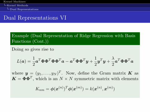
Dual Representations VI
Example (Dual Representation of Ridge Regression with BasisFunctions (Cont.))
Doing so gives rise to
L(a) =1
2aTΦΦTΦΦTa− aTΦΦTy +
1
2yTy +
λ
2aTΦΦTa
where y = (y1, . . . , yN )T . Now, define the Gram matrix K asK = ΦΦT , which is an N ×N symmetric matrix with elements
Knm = φ(x(n))Tφ(x(m)) = k(x(n),x(m))

Kernel Machines
Kernel Methods
Dual Representations
Dual Representations VII
Example (Dual Representation of Ridge Regression with BasisFunctions (Cont.))
Now, writing the regularised sum-of-squares in terms of K yields
L(a) =1
2aTKKTa− aTKy +
1
2yTy +
λ
2aTKa
Thus we see that the dual formulation allows the solution to theleast-squares problem to be expressed entirely in terms of thekernel function k(x(n),x(m)).
Kernel Machines
Kernel Methods
Dual Representations
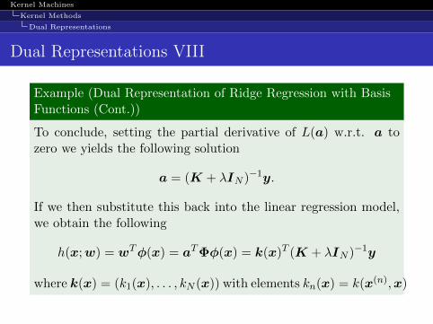
Dual Representations VIII
Example (Dual Representation of Ridge Regression with BasisFunctions (Cont.))
To conclude, setting the partial derivative of L(a) w.r.t. a tozero we yields the following solution
a = (K + λIN )−1y.
If we then substitute this back into the linear regression model,we obtain the following
h(x;w) = wTφ(x) = aTΦφ(x) = k(x)T (K + λIN )−1y
where k(x) = (k1(x), . . . , kN (x)) with elements kn(x) = k(x(n),x)

Kernel Machines
Kernel Methods
Constructing Kernels
Constructing Kernels I
In order to exploit the kernel trick, we need to be able to constructvalid kernel functions. Generally, there are two approaches:
1 Choose a feature space mapping φ(x) and then use this tofind the corresponding kernel function.
2 Construct the kernel function directly.

Kernel Machines
Kernel Methods
Constructing Kernels
Constructing Kernels II
Example (From Feature Map to Kernel)
Suppose that we want to find the kernel which corresponds tothe following feature mapping φ(x) = (1, x1, x2, x1x2)
T then, thekernel corresponding to this feature mapping is
k(x,x′) = φ(x)Tφ(x′)
= (1, x1, x2, x1x2)T (1, x′1, x
′2, x′1x′2)
= 1 + x′1 + x′2 + x′1x′2
+ x1 + x1x′1 + x1x
′2 + x1x
′1x′2
+ x2 + x2x′1 + x2x
′2 + x2x
′1x′2
+ x1x2 + x1x2x′1 + x1x2x
′2 + x1x2x
′1x′2.
Kernel Machines
Kernel Methods
Constructing Kernels
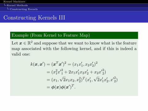
Constructing Kernels III
Example (From Kernel to Feature Map)
Let x ∈ R2 and suppose that we want to know what is the featuremap associated with the following kernel, and if this is indeed avalid one:
k(x,x′) = (xTx′)2 = (x1x′1, x2x
′2)
2
= (x21x′21 + 2x1x
′1x2x
′2 + x2x
′22)
= (x1,√
2x1x2, x22)T (x′1,
√2x′1x
′2, x′22)
= φ(x)φ(x′)T .

Kernel Machines
Kernel Methods
Constructing Kernels
Constructing Kernels IV
Example (From Kernel to Feature Map (Cont.))
We see that the feature mapping takes the form
φ(x) = (x1,√
2x1x2, x22)T .
and therefore comprises all possible second order terms, with aspecific weighting between them. Furthermore, we can see thatthe kernel can be written in terms of an inner product in s spacedefined by φ(x).
Kernel Machines
Kernel Methods
Constructing Kernels
Constructing Kernels V
More generally, however, we need a simple way to test whethera function constitutes a valid kernel without having to constructthe function φ(x) explicitly.

Kernel Machines
Kernel Methods
Constructing Kernels
Constructing Kernels VI
Result
A necessary and sufficient condition for a function k(x(n),x(m))to be a valid kernel (Shawe Taylor and Cristianini, 2004) is thatthe Gram matrix K, whose elements are given by k(x(n),x(m)),should be positive semi-definite for all possible choices of the set{x(n),x(m)}
Kernel Machines
Kernel Methods
Constructing Kernels
Constructing Kernels VII
Therefore, we can use a kernel k(·, ·) without having to do anycalculation in the underlying feature space !

Kernel Machines
Kernel Methods
Constructing Kernels
Constructing Kernels VIII
Result (Gaussian Kernel)
Consider the Gaussian kernel, which belongs to the class of RadialBasis Function (RBF) kernels
k(x,x′) = exp(− γ||x− x′||2
)then, the underlying space is infinite dimensional.

Kernel Machines
Kernel Methods
Constructing Kernels
Constructing Kernels IX
Proof.
Take the case where x ∈ R and γ = 1 then,
k(x, x′) = exp(− (x− x′)2
)= exp(x2) exp(x′
2) exp(2xx′)
= exp(x2) exp(x′2)
∞∑k=0
2k(x)k(x′)k
k!
= exp(x2)
∞∑k=0
2k2 (x)k√k!
exp(x′2)
∞∑k=0
2k2 (x′)k√k!

Kernel Machines
Kernel Methods
Constructing Kernels
Constructing Kernels X
One powerful technique for constructing new kernels is to buildthem out of simpler kernels as building blocks. This can be doneusing the following properties.Let c > 0 be a constant, f(·) any function, q(·) a polynomial withnon-negative coefficients, φ : RD → RM , k3(·, ·) a valid kernel inRM , and A a positive semidefinite matrix.

Kernel Machines
Kernel Methods
Constructing Kernels
Constructing Kernels XI
Given valid kernels k1(x,x′) and k2(xx
′) the following are alsovalid kernels
k(x,x′) = ck1(x,x′)
k(x,x′) = f(x)k1(x,x′)f(x′)
k(x,x′) = q(k1(x,x′))
k(x,x′) = exp(k1(x,x′))
k(x,x′) = k1(x,x′) + k2(x,x
′)
k(x,x′) = k1(x,x′)k2(x,x
′)
k(x,x′) = k3(φ(x),φ(x′))
k(x,x′) = xTAx′

Kernel Machines
Support Vector Machines For Classification
Outline I
1 IntroductionTraining DataLoss FunctionsGeneralisation And Overfitting
2 Kernel MethodsKernel Methods: An IntroductionDual RepresentationsConstructing Kernels
3 Support Vector Machines For ClassificationSupport Vector Machines For Classification: An OverviewHard Margin SVMs For ClassificationSoft Margin SVMs For ClassificationA Note on ComputationsA Note on Probabilistic Output

Kernel Machines
Support Vector Machines For Classification
Outline II
A Note on Multiclass Problems
4 Support Vector Machines For RegressionSupport Vector Machines For Regression: An OverviewCommon Kernels Choices
Kernel Machines
Support Vector Machines For Classification
Support Vector Machines For Classification: An Overview
An Overview I
Support Vector Machines (SVMs) belong to a class of non prob-abilistic classification models called maximum margin classifiers.
Definition (Margin)
We define the margin as the smallest distance between the deci-sion boundary and any of the samples.

Kernel Machines
Support Vector Machines For Classification
Support Vector Machines For Classification: An Overview
An Overview II
An important property of support vector machines is that thedetermination of the model parameters corresponds to a convexoptimization problem, and so any local solution is also a globaloptimum.

Kernel Machines
Support Vector Machines For Classification
Hard Margin SVMs For Classification
Hard Margin SVMs For Classification I
Consider the class of linear models for binary classification prob-lems specified by
h(x) = wTφ(x) + b
where φ : RD → RM denotes a fixed feature-space transforma-tion, and b ∈ R denotes the bias term.

Kernel Machines
Support Vector Machines For Classification
Hard Margin SVMs For Classification
Hard Margin SVMs For Classification II
Consider a data set given by
{(x(n), y(n)) ∈ RD × {−1,+1} | n = 1, . . . , N},
and assume that is it linearly separable in the feature space spec-ified by φ : RD → RM .

Kernel Machines
Support Vector Machines For Classification
Hard Margin SVMs For Classification
Hard Margin SVMs For Classification III
by definition of linear separability, there exist at least one choiceof the parameters w and b such that
h(x(n)) = wTφ(x(n)) + b =
{> 0 if y(n) = +1
< 0 if y(n) = −1
So that
h(x(n))y(n) > 0
for all training data points.

Kernel Machines
Support Vector Machines For Classification
Hard Margin SVMs For Classification
Hard Margin SVMs For Classification IV
In support vector machines the decision boundary is cho-sen to be the one for which the margin is maximized.
The maximum margin solution can be motivated using computa-tional learning theory, also known as statistical learning theory.
Kernel Machines
Support Vector Machines For Classification
Hard Margin SVMs For Classification
Hard Margin SVMs For Classification V
the perpendicular distance of a point x from a hyperplane definedby h(x) = 0 where h(x) = wTφ(x) + b is given by
|h(x)|||w||2
.
Furthermore, we are only interested in solutions for which alldata points are correctly classified, so that h(x(n))y(n) > 0

Kernel Machines
Support Vector Machines For Classification
Hard Margin SVMs For Classification
Hard Margin SVMs For Classification VI
Thus the distance of an observation x(n) to the decision surfaceunder perfect classification is given by
|h(x(n))y(n)|||w||2
=|(wTφ(x(n)) + b)y(n)|
||w||2

Kernel Machines
Support Vector Machines For Classification
Hard Margin SVMs For Classification
Hard Margin SVMs For Classification VII
The margin, is the perpendicular distance to the closest pointx(n) from decision boundary. Thus, the maximum margin solu-tion is found by solving
arg maxw,b
{ 1
||w||2minn{(wTφ(x(n)) + b)y(n)}
}.

Kernel Machines
Support Vector Machines For Classification
Hard Margin SVMs For Classification
Hard Margin SVMs For Classification VIII
Direct solutions to this optimisation problem would be very com-plex, and so we shall impose that
(wTφ(x(n)) + b)y(n) = 1
for the point that is closest to the surface. So that, all data pointswill satisfy the constraints
(wTφ(x(n)) + b)y(n) ≥ 1, ∀ n = 1, 2, . . . , N.

Kernel Machines
Support Vector Machines For Classification
Hard Margin SVMs For Classification
Hard Margin SVMs For Classification IX
So, the optimisation problem that needs to be solved is given by
arg maxw,b
1
||w||2s.t. (wTφ(x(n)) + b)y(n) ≥ 1, ∀ n = 1, 2, . . . , N.
which is equivalent to
arg minw,b
1
2||w||22
s.t. (wTφ(x(n)) + b)y(n) ≥ 1, ∀ n = 1, 2, . . . , N.

Kernel Machines
Support Vector Machines For Classification
Hard Margin SVMs For Classification
Hard Margin SVMs For Classification X
The above optimisation problem is an example of a quadraticprogramming problem in which we are minimizing a quadraticfunction subject to a set of linear inequality constraints.

Kernel Machines
Support Vector Machines For Classification
Hard Margin SVMs For Classification
Hard Margin SVMs For Classification XI
In order to solve this constrained optimization problem, we in-troduce Lagrange multipliers {αn ≥ 0}Nn=1, giving the Lagrangefunction
L(w,α, b) =1
2||w||22 −
N∑n=1
αn((wTφ(x(n)) + b)y(n) − 1)
where α = (α1, α2, . . . , αN )T . Note the minus sign is in front ofthe Lagrangian multipliers because we are minimising w.r.t. wand b, but we are maximising with respect to α since we want asthe classifications to be correct, that is we want
(wTφ(x(n)) + b)y(n) ≥ 1.
Kernel Machines
Support Vector Machines For Classification
Hard Margin SVMs For Classification
Hard Margin SVMs For Classification XII
Setting the derivatives of L(w,α, b) with respect tow and b equalto zero, we obtain the following two conditions
∂L(w,α, b)
∂w= 0 =⇒ w =
N∑n=1
αnφ(x(n))y(n)
∂L(w,α, b)
∂b= 0 =⇒ 0 =
N∑n=1
αny(n).

Kernel Machines
Support Vector Machines For Classification
Hard Margin SVMs For Classification
Hard Margin SVMs For Classification XIII
Using the conditions above to get rid of the dependencies onw and b from L(w,α, b) leads to the dual formulation of theoptimisation problem:
arg maxα
N∑n=1
αn −1
2
N∑n=1
N∑m=1
αnαmφ(x(n))Tφ(x(m))y(n)y(m)
s.t. αn ≥ 0, ∀ n = 1, 2, . . . , N,
N∑n=1
αny(n) = 0.

Kernel Machines
Support Vector Machines For Classification
Hard Margin SVMs For Classification
Hard Margin SVMs For Classification XIV
We note that the data enters the function to optimise only inthe form of an inner product in the feature space specified byφ : RD → RM . Hence, we can apply the kernel trick by replacingφ(x(n))Tφ(x(m)) with
k(x(n),x(m)).

Kernel Machines
Support Vector Machines For Classification
Hard Margin SVMs For Classification
Hard Margin SVMs For Classification XV
In order to classify new data points using the trained model, weevaluate the sign of h(x) = wTφ(x) + b which can be expressedin terms of the kernel function and the Lagrange multipliers bysubstituting for
w =N∑n=1
αnφ(x(n))y(n)
giving
h(x) =
N∑n=1
αnk(x,x(n))y(n) + b.
Kernel Machines
Support Vector Machines For Classification
Hard Margin SVMs For Classification
Hard Margin SVMs For Classification XVI
Result (Hard Margin SVM)
Consider an Hard Margin SVM where the decision boundary ismodelled as
h(x) = wTφ(x) + b,
where φ : RD → RM denotes a fixed feature-space transforma-tion, and b ∈ R denotes the bias term. Let the training data beof the form
{(x(n), y(n)) ∈ RD × {−1,+1} | n = 1, . . . , N}.

Kernel Machines
Support Vector Machines For Classification
Hard Margin SVMs For Classification
Hard Margin SVMs For Classification XVII
Result (Hard Margin SVM (Cont.))
Assume that the data is linearly separable in the feature spacespecified by φ, and impose that
(wTφ(x(n)) + b)y(n) ≥ 1, ∀ n = 1, 2, . . . , N.

Kernel Machines
Support Vector Machines For Classification
Hard Margin SVMs For Classification
Hard Margin SVMs For Classification XVIII
Result (Hard Margin SVM (Cont.))
Then, the set of parameters w and b which achieve perfect clas-sification can be found by solving the dual problem given by
arg maxα
N∑n=1
αn −1
2
N∑n=1
N∑m=1
αnαmk(x(n),x(m))y(n)y(m)
s.t. αn ≥ 0, ∀ n = 1, 2, . . . , N,
N∑n=1
αny(n) = 0.
(3.1)
where k(x(n),x(m)) is a valid kernel.

Kernel Machines
Support Vector Machines For Classification
Hard Margin SVMs For Classification
Hard Margin SVMs For Classification XIX
Result (Hard Margin SVM (Cont.))
Finally, we can make predictions by computing
h(x) =
N∑n=1
αnk(x,x(n))y(n) + b.

Kernel Machines
Support Vector Machines For Classification
Soft Margin SVMs For Classification
Soft Margin SVMs For Classification I
So far, we have assumed that the training data points are linearlyseparable in the feature space given by φ.In practice, however, the training data might not be linearly sep-arable neither in the input nor in the feature space.
Kernel Machines
Support Vector Machines For Classification
Soft Margin SVMs For Classification
Soft Margin SVMs For Classification II
Question: How can we deal with data that is not linearly sepa-rable neither in the input nor in the feature space?

Kernel Machines
Support Vector Machines For Classification
Soft Margin SVMs For Classification
Soft Margin SVMs For Classification III
Answer: Modify the support vector machine so as to allow someof the training points to be misclassified.
Kernel Machines
Support Vector Machines For Classification
Soft Margin SVMs For Classification
Soft Margin SVMs For Classification IV
To do so we introduce the slack variables ξn ≥ 0 to allow formisclassification errors to occur. That is, we allow non linearlyseparable dataset to be dealt with.These are defined as
ξn = 0, if x(n) is on or inside the correct margin boundary
ξn = |y(n) − h(x(n))| if x(n) is not on or inside the correctmargin boundary
Note: ξn can be greater than 0 even thought the nth observationis on the correct side of the decision boundary if it is inside themargin.
Kernel Machines
Support Vector Machines For Classification
Soft Margin SVMs For Classification
Soft Margin SVMs For Classification V
The exact classification constraints are then replaced with
h(x(n))y(n) ≥ 1− ξn, n = 1, 2, . . . , N.
in which the slack variables are constrained to satisfy ξn ≥ 0.
Kernel Machines
Support Vector Machines For Classification
Soft Margin SVMs For Classification
Soft Margin SVMs For Classification VI
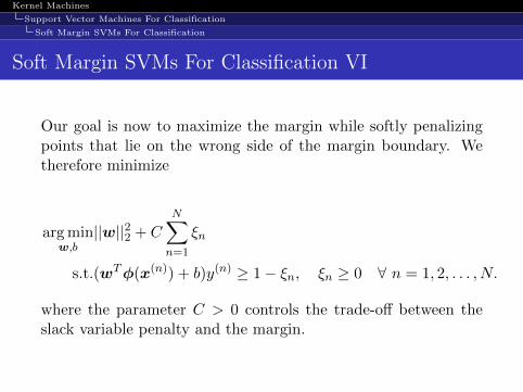
Our goal is now to maximize the margin while softly penalizingpoints that lie on the wrong side of the margin boundary. Wetherefore minimize
arg minw,b
||w||22 + CN∑n=1
ξn
s.t.(wTφ(x(n)) + b)y(n) ≥ 1− ξn, ξn ≥ 0 ∀ n = 1, 2, . . . , N.
where the parameter C > 0 controls the trade-off between theslack variable penalty and the margin.
Kernel Machines
Support Vector Machines For Classification
Soft Margin SVMs For Classification
Soft Margin SVMs For Classification VII
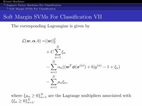
The corresponding Lagrangian is given by
L(w,α, b) =||w||22
+ C
N∑n=1
ξn
−N∑n=1
αn((wTφ(x(n)) + b)y(n) − 1 + ξn)
−N∑n=1
µnξn,
where {µn ≥ 0}Nn=1 are the Lagrange multipliers associated with{ξn ≥ 0}Nn=1.
Kernel Machines
Support Vector Machines For Classification
Soft Margin SVMs For Classification
Soft Margin SVMs For Classification VIII
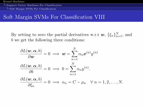
By setting to zero the partial derivatives w.r.t w, {ξn}Nn=1, andb we get the following three conditions:
∂L(w,α, b)
∂w= 0 =⇒ w =
N∑n=1
αnx(n)y(n)
∂L(w,α, b)
∂b= 0 =⇒ 0 =
N∑n=1
αny(n).
∂L(w,α, b)
∂ξn= 0 =⇒ αn = C − µn ∀ n = 1, 2, . . . , N.

Kernel Machines
Support Vector Machines For Classification
Soft Margin SVMs For Classification
Soft Margin SVMs For Classification IX
Using these conditions to get rid of the dependencies on w and bfrom L(w,α, b) leads to the dual formulation of the optimisationproblem:
arg maxα
N∑n=1
αn −1
2
N∑n=1
N∑m=1
αnαmφ(x(n))Tφ(x(m))y(n)y(m)
s.t. 0 ≤ αn ≤ C,N∑n=1
αny(n) = 0
∀ n = 1, 2, . . . , N.
Kernel Machines
Support Vector Machines For Classification
Soft Margin SVMs For Classification
Soft Margin SVMs For Classification X
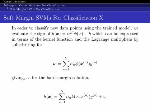
In order to classify new data points using the trained model, weevaluate the sign of h(x) = wTφ(x) + b which can be expressedin terms of the kernel function and the Lagrange multipliers bysubstituting for
w =
N∑n=1
αnφ(x(n))y(n)
giving, as for the hard margin solution,
h(x) =
N∑n=1
αnk(x,x(n))y(n) + b.
Kernel Machines
Support Vector Machines For Classification
Soft Margin SVMs For Classification
Soft Margin SVMs For Classification XI
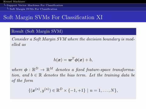
Result (Soft Margin SVM)
Consider a Soft Margin SVM where the decision boundary is mod-elled as
h(x) = wTφ(x) + b,
where φ : RD → RM denotes a fixed feature-space transforma-tion, and b ∈ R denotes the bias term. Let the training data beof the form
{(x(n), y(n)) ∈ RD × {−1,+1} | n = 1, . . . , N},
Kernel Machines
Support Vector Machines For Classification
Soft Margin SVMs For Classification
Soft Margin SVMs For Classification XII
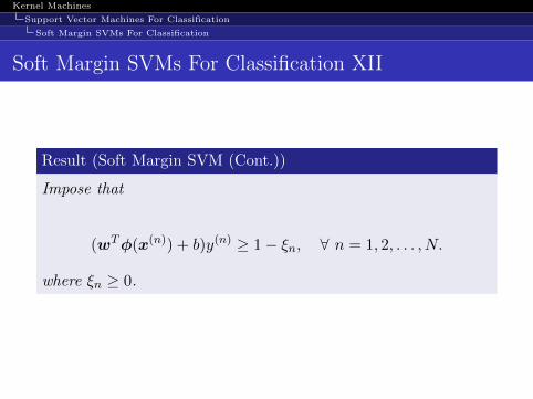
Result (Soft Margin SVM (Cont.))
Impose that
(wTφ(x(n)) + b)y(n) ≥ 1− ξn, ∀ n = 1, 2, . . . , N.
where ξn ≥ 0.

Kernel Machines
Support Vector Machines For Classification
Soft Margin SVMs For Classification
Soft Margin SVMs For Classification XIII
Result (Soft Margin SVM (Cont.))
Then, the set of parameters w and b can be found by solving thedual problem given by
arg maxα
N∑n=1
αn −1
2
N∑n=1
N∑m=1
αnαmk(x(n),x(m))y(n)y(m)
s.t. 0 ≤ αn ≤ C,N∑n=1
αny(n) = 0
∀ n = 1, 2, . . . , N.
(3.2)
where k(x(n),x(m)) is a valid kernel.

Kernel Machines
Support Vector Machines For Classification
Soft Margin SVMs For Classification
Soft Margin SVMs For Classification XIV
Result (Soft Margin SVM (Cont.))
Finally, we can make predictions by computing
h(x) =
N∑n=1
αnk(x,x(n))y(n) + b.
Kernel Machines
Support Vector Machines For Classification
A Note on Computations
A Note on Computations I
We first note that the objective function given by 3.1 or 3.2 isquadratic and so any local optimum will also be a global optimumsince the constraints define a convex region as a consequence ofbeing liner.
Kernel Machines
Support Vector Machines For Classification
A Note on Computations
A Note on Computations II
Direct solution of the quadratic programming problem using tra-ditional techniques is often infeasible due to the demanding com-putation and memory requirements.So, a wide range of more practical approaches have been pro-posed:
Protected conjugate gradients (Burges, 1998).
Decomposition methods (Osuna et al., 1996).
Sequential minimal optimization (Platt, 1999).
Kernel Machines
Support Vector Machines For Classification
A Note on Probabilistic Output
Support Vector Machines: A Note on ProbabilisticOutput I
As we have seen, support vector machines do not provide proba-bilistic outputs but instead make hard classification decisions fornew input vectors.However, it is possible to construct conditional probabilities ofthe form
P(y = 1|x) = 1− P(y = −1|x)
by fitting a logistic sigmoid to the outputs of a previously trainedSVM Platt (2000).

Kernel Machines
Support Vector Machines For Classification
A Note on Probabilistic Output
Support Vector Machines: A Note on ProbabilisticOutput II
Specifically, the conditional probability is assumed to be of theform
P(y = 1|x; w) = σ(w0 + w1h(x))
where the parameters w = (w0, w1) ∈ R2 are found by minimis-ing the negative log-likelihood of the training data:
− logP(y|w,X) = −N∑n=1
(y(n) logP(y(n) = 1|w,x(n))
+(1− y(n)) log(1− P(y(n) = 1|w,x(n)))
Kernel Machines
Support Vector Machines For Classification
A Note on Probabilistic Output
Support Vector Machines: A Note on ProbabilisticOutput III
Note: it is important to fit the logistic model using data thathas not been used to train the underlying SVM in order to avoidsevere overfitting.

Kernel Machines
Support Vector Machines For Classification
A Note on Multiclass Problems
Support Vector Machines: A Note on MulticlassProblems I
The support vector machine is fundamentally a two-class clas-sifier. In practice, however, we often have to tackle problemsinvolving K > 2 classes. Various methods have therefore beenproposed for combining multiple two-class SVMs in order to builda multiclass classifier.
Kernel Machines
Support Vector Machines For Classification
A Note on Multiclass Problems
Support Vector Machines: A Note on MulticlassProblems II
one-versus-the-rest: train K separate SVMs, in which thekth model hk(x) is trained using the data from class Ck asthe positive examples and the data from the remainingK − 1 classes as the negative examples.
one-versus-one: train K(K − 1)/2 different 2-class SVMson all possible pairs of classes, and then to classify testpoints according to which class has the highest number ofvotes.

Kernel Machines
Support Vector Machines For Regression
Outline I
1 IntroductionTraining DataLoss FunctionsGeneralisation And Overfitting
2 Kernel MethodsKernel Methods: An IntroductionDual RepresentationsConstructing Kernels
3 Support Vector Machines For ClassificationSupport Vector Machines For Classification: An OverviewHard Margin SVMs For ClassificationSoft Margin SVMs For ClassificationA Note on ComputationsA Note on Probabilistic Output
Kernel Machines
Support Vector Machines For Regression
Outline II
A Note on Multiclass Problems
4 Support Vector Machines For RegressionSupport Vector Machines For Regression: An OverviewCommon Kernels Choices
Kernel Machines
Support Vector Machines For Regression
Support Vector Machines For Regression: An Overview
Support Vector Machines For Regression: An Overview
We now extend support vector machines to regression problemswhile at the same time preserving the property of sparseness.In regularised linear regression, the objective is to minimise theregularised error function given by
1
2
N∑n=1
(h(x(n))− y(n))2 +λ
2||w||22
where λ ≥ 0 determines the regularisation strength.Support vector regression replaces the sum-of-squared error func-tion with an ε- insensitive error function in order to recoversparse solutions.
Kernel Machines
Support Vector Machines For Regression
Support Vector Machines For Regression: An Overview
Derivation I
Let us take a special case of an ε- insensitive error function hav-ing a linear cost associated with errors outside the insensitiveregion
Eε(h(x;w)− y) =
{0, if |h(x;w)− y| < ε
|h(x;w)− y| − ε, otherwise
This error function gives zero error if the absolute difference be-tween the predicted value h(x;w) and the target y is less than εwhere ε > 0.
Kernel Machines
Support Vector Machines For Regression
Support Vector Machines For Regression: An Overview
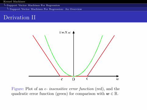
Derivation II
Figure: Plot of an ε- insensitive error function (red), and thequadratic error function (green) for comparison with w ∈ R.
Kernel Machines
Support Vector Machines For Regression
Support Vector Machines For Regression: An Overview
Derivation III
Given the model family expressed as
h(x) = wTφ(x) + b
where φ : RD → RM denotes a fixed feature-space transforma-tion,we therefore want to find the weights w ∈ RD and b which min-imize the regularized error function given by
C
N∑n=1
Eε(h(x(n))− y(n)) +1
2||w||22
Kernel Machines
Support Vector Machines For Regression
Support Vector Machines For Regression: An Overview
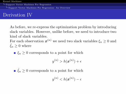
Derivation IV
As before, we re-express the optimization problem by introducingslack variables. However, unlike before, we need to introduce twokind of slack variables.For each observation x(n) we need two slack variables ξn ≥ 0 andξn ≥ 0 where
ξn ≥ 0 corresponds to a point for which
y(n) > h(x(n)) + ε
ξn ≥ 0 corresponds to a point for which
y(n) < h(x(n))− ε
Kernel Machines
Support Vector Machines For Regression
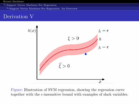
Support Vector Machines For Regression: An Overview
Derivation V
Figure: Illustration of SVM regression, showing the regression curvetogether with the ε-insensitive bound with examples of slack variables.

Kernel Machines
Support Vector Machines For Regression
Support Vector Machines For Regression: An Overview
Derivation VI
The condition for a target point to lie inside the ε-tube is that
h(x(n))− ε ≥ y(n) ≤ h(x(n)) + ε.
Introducing the slack variables allows points to lie outside thetube provided the slack variables are non-zero, and the corre-sponding conditions are
y(n) ≤ h(x(n)) + ε+ ξn,
y(n) ≥ h(x(n))− ε− ξn.
Kernel Machines
Support Vector Machines For Regression
Support Vector Machines For Regression: An Overview
Derivation VII
The error function for support vector regression can then be writ-ten as
C
N∑n=1
(ξn + ξn)− y(n)) +1
2||w||22.

Kernel Machines
Support Vector Machines For Regression
Support Vector Machines For Regression: An Overview
Derivation VIII
From this, we can write the optimisation problem as
arg maxw
C
N∑n=1
(ξn + ξn)− y(n)) +1
2||w||22
s.t. ξn ≥ 0,
ξn ≥ 0,
y(n) ≤ h(x(n)) + ε+ ξn,
y(n) ≥ h(x(n))− ε− ξn,∀ n = 1, 2, . . . , N.

Kernel Machines
Support Vector Machines For Regression
Support Vector Machines For Regression: An Overview
Derivation IX
In order to solve this constrained optimization problem, we in-troduce Lagrange multipliers {αn ≥ 0}Nn=1, {αn ≥ 0}Nn=1, {µn ≥0}Nn=1, and {µn ≥ 0}Nn=1 giving the Lagrange function

Kernel Machines
Support Vector Machines For Regression
Support Vector Machines For Regression: An Overview
Derivation X
L =C
N∑n=1
(ξn + ξn) +1
2||w||22
−N∑n=1
(µnξn + µnξn)
−N∑n=1
αn(ε+ ξn + h(x)− y(n))
−N∑n=1
αn(ε+ ξn − h(x) + y(n)).
Kernel Machines
Support Vector Machines For Regression
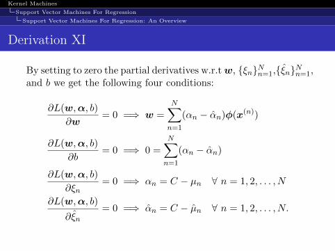
Support Vector Machines For Regression: An Overview
Derivation XI
By setting to zero the partial derivatives w.r.tw, {ξn}Nn=1,{ξn}Nn=1,and b we get the following four conditions:
∂L(w,α, b)
∂w= 0 =⇒ w =
N∑n=1
(αn − αn)φ(x(n))
∂L(w,α, b)
∂b= 0 =⇒ 0 =
N∑n=1
(αn − αn)
∂L(w,α, b)
∂ξn= 0 =⇒ αn = C − µn ∀ n = 1, 2, . . . , N
∂L(w,α, b)
∂ξn= 0 =⇒ αn = C − µn ∀ n = 1, 2, . . . , N.

Kernel Machines
Support Vector Machines For Regression
Support Vector Machines For Regression: An Overview
Derivation XII
Using these conditions to get rid of the dependencies on w and bfrom L leads to the dual formulation of the optimisation problem:
arg minα,α
− 1
2
N∑n=1
N∑m=1
(αn − αn)(αm − αm)k(xn,xm)
s.t. 0 ≤ αn ≤ C,0 ≤ αn ≤ C,N∑n=1
(αn − αn) = 0
∀ n = 1, 2, . . . , N.
where we have introduced the kernel k(xn,xm) = φ(x(n))Tφ(x(m)).

Kernel Machines
Support Vector Machines For Regression
Support Vector Machines For Regression: An Overview
Derivation XIII
In order to classify new data points using the trained model, weevaluate the sign of h(x) = wTφ(x) + b which can be expressedin terms of the kernel function and the Lagrange multipliers bysubstituting for
w =N∑n=1
(αn − αn)φ(x(n))
giving
h(x) =
N∑n=1
(αn − αn)k(x,xn) + b.

Kernel Machines
Support Vector Machines For Regression
Support Vector Machines For Regression: An Overview
Derivation XIV
Result (Support Vector Regression)
Consider a support vector regression model where specified as
h(x) = wTφ(x) + b,
where φ : RD → RM denotes a fixed feature-space transforma-tion, and b ∈ R denotes the bias term. Let the training data beof the form
{(x(n), y(n)) ∈ RD × R | n = 1, . . . , N}.

Kernel Machines
Support Vector Machines For Regression
Support Vector Machines For Regression: An Overview
Derivation XV
Result (Hard Margin SVM (Cont.))
Impose that
y(n) ≤ h(x(n)) + ε+ ξn,
y(n) ≥ h(x(n))− ε− ξn.
where {ξn ≥ 0}Nn=1, {ξn ≥ 0}Nn=1, and ε > 0
Kernel Machines
Support Vector Machines For Regression
Support Vector Machines For Regression: An Overview
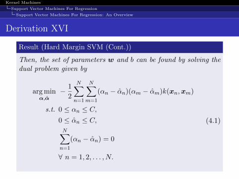
Derivation XVI
Result (Hard Margin SVM (Cont.))
Then, the set of parameters w and b can be found by solving thedual problem given by
arg minα,α
− 1
2
N∑n=1
N∑m=1
(αn − αn)(αm − αm)k(xn,xm)
s.t. 0 ≤ αn ≤ C,0 ≤ αn ≤ C,N∑n=1
(αn − αn) = 0
∀ n = 1, 2, . . . , N.
(4.1)

Kernel Machines
Support Vector Machines For Regression
Support Vector Machines For Regression: An Overview
Derivation XVII
Result (Hard Margin SVM (Cont.))
where k(x(n),x(m)) is a valid kernel.Finally, we can make predictions by computing
h(x) =
N∑n=1
(αn − αn)k(x,xn) + b.
Kernel Machines
Support Vector Machines For Regression
Common Kernels Choices
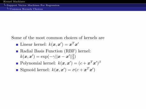
Some of the most common choices of kernels are
Linear kernel: k(x,x′) = xTx′
Radial Basis Function (RBF) kernel:k(x,x′) = exp(−γ||x− x′||22)Polynomial kernel: k(x,x′) = (c+ xTx′)β
Sigmoid kernel: k(x,x′) = σ(c+ xTx′)
Kernel Machines
Appendix
For Further Reading
For Further Reading I
Shawe-Taylor, J. and N. Cristianini (2004)Kernel Methods for Pattern Analysis.Cambridge University Press.
Aizerman, M. A., E. M. Braverman, and L. I. Rozonoer(1964)The probability problem of pattern recognition learning andthe method of potential functionsAutomation and Remote Control, 25:1175–1190.
Boser, B. E., I. M. Guyon, and V. N. Vapnik (1992)A training algorithm for optimal margin classi- fiers. In D.Haussler (Ed.)Proceedings Fifth Annual Workshop on ComputationalLearning Theory (COLT), 144–152.

Kernel Machines
Appendix
For Further Reading
For Further Reading II
Cortes, C. and V. N. Vapnik (1995)Support vector networksMachine Learning, 20: 273-297.