Embed Size (px)
Citation preview

Kernels and the learning problem Tools: the functional framework Algorithms Conclusion
Plan
1 Kernels and the learning problemThree learning problemsLearning from data: the problemKernelizing the linear regressionKernel machines: a definition
2 Tools: the functional frameworkIn the beginning was the kenrelKernel and hypothesis setOptimization, loss function and the reguarization cost
3 Kernel machinesNon sparse kernel machinessparse kernel machines: SVMpractical SVM
4 Conclusion

Kernels and the learning problem Tools: the functional framework Algorithms Conclusion
Interpolation splines
find out f ∈ H such that f (xi ) = yi , i = 1, ..., n
It is an ill posed problem

Kernels and the learning problem Tools: the functional framework Algorithms Conclusion
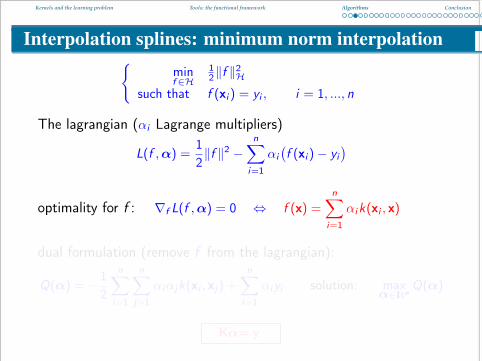
Interpolation splines: minimum norm interpolation{minf∈H
12‖f ‖
2H
such that f (xi ) = yi , i = 1, ..., n
The lagrangian (αi Lagrange multipliers)
L(f ,α) =12‖f ‖2 −
n∑i=1
αi(f (xi )− yi
)
optimality for f : ∇f L(f ,α) = 0 ⇔ f (x) =n∑
i=1
αik(xi , x)
dual formulation (remove f from the lagrangian):
Q(α) = −12
n∑i=1
n∑j=1
αiαjk(xi , xj) +n∑
i=1
αiyi solution: maxα∈IRn
Q(α)
Kα= y
Kernels and the learning problem Tools: the functional framework Algorithms Conclusion
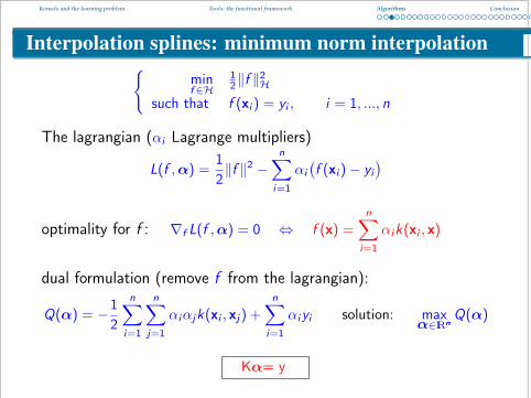
Interpolation splines: minimum norm interpolation{minf∈H
12‖f ‖
2H
such that f (xi ) = yi , i = 1, ..., n
The lagrangian (αi Lagrange multipliers)
L(f ,α) =12‖f ‖2 −
n∑i=1
αi(f (xi )− yi
)
optimality for f : ∇f L(f ,α) = 0 ⇔ f (x) =n∑
i=1
αik(xi , x)
dual formulation (remove f from the lagrangian):
Q(α) = −12
n∑i=1
n∑j=1
αiαjk(xi , xj) +n∑
i=1
αiyi solution: maxα∈IRn
Q(α)
Kα= y
Kernels and the learning problem Tools: the functional framework Algorithms Conclusion
Interpolation splines: minimum norm interpolation{minf∈H
12‖f ‖
2H
such that f (xi ) = yi , i = 1, ..., n
The lagrangian (αi Lagrange multipliers)
L(f ,α) =12‖f ‖2 −
n∑i=1
αi(f (xi )− yi
)
optimality for f : ∇f L(f ,α) = 0 ⇔ f (x) =n∑
i=1
αik(xi , x)
dual formulation (remove f from the lagrangian):
Q(α) = −12
n∑i=1
n∑j=1
αiαjk(xi , xj) +n∑
i=1
αiyi solution: maxα∈IRn
Q(α)
Kα= y

Kernels and the learning problem Tools: the functional framework Algorithms Conclusion
Representer theorem
Theorem (epresenter theorem)LetH be a RKHS with kernel k(s, t). Let ` be a function from X to IR(loss function) and Φ a non decreasing function from IR to IR. If thereexists a function f ∗minimizing:
f ∗ = argminf∈H
n∑i=1
`(yi , f (xi )
)+ Φ
(‖f ‖2H
)then there exists a vector α ∈ IRn such that:
f ∗(x) =n∑
i=1
αik(x, xi )
it can be generalized to the semi parametric case: +∑m
j=1 βjφj(x)
Kernels and the learning problem Tools: the functional framework Algorithms Conclusion
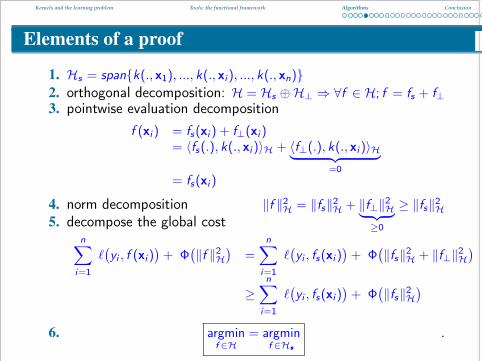
Elements of a proof
1. Hs = span{k(., x1), ..., k(., xi ), ..., k(., xn)}2. orthogonal decomposition: H = Hs ⊕H⊥ ⇒ ∀f ∈ H; f = fs + f⊥3. pointwise evaluation decomposition
f (xi ) = fs(xi ) + f⊥(xi )= 〈fs(.), k(., xi )〉H + 〈f⊥(.), k(., xi )〉H︸ ︷︷ ︸
=0= fs(xi )
4. norm decomposition ‖f ‖2H = ‖fs‖2H + ‖f⊥‖2H︸ ︷︷ ︸≥0
≥ ‖fs‖2H5. decompose the global cost
n∑i=1
`(yi , f (xi )
)+ Φ
(‖f ‖2H
)=
n∑i=1
`(yi , fs(xi )
)+ Φ
(‖fs‖2H + ‖f⊥‖2H
)≥
n∑i=1
`(yi , fs(xi )
)+ Φ
(‖fs‖2H
)6. argmin
f∈H= argmin
f∈Hs
.

Kernels and the learning problem Tools: the functional framework Algorithms Conclusion
Smooting splinesintroducing the error (the slack) ξ = f (xi )− yi
(S)
minf∈H
12‖f ‖
2H + 1
2λ
n∑i=1
ξ2i
such that f (xi ) = yi + ξi , i = 1, n
three equivalents definitions(S′) min
f∈H
12
n∑i=1
(f (xi )− yi
)2+λ
2‖f ‖2H
minf∈H
12‖f ‖
2H
such thatn∑
i=1
(f (xi )− yi
)2 ≤ C ′
minf∈H
n∑i=1
(f (xi )− yi
)2such that ‖f ‖2H ≤ C ′′
using the representer theorem(S ′′) min
α∈IRn
12‖Kα− y‖2 +
λ
2α>Kα
solution:(S)⇔ (S ′)⇔ (S ′′)⇔ (K + λI )α = y
minα∈IRn
12‖Kα− y‖2 +
λ
2α>α
α = (K>K + λI )−1K>y

Kernels and the learning problem Tools: the functional framework Algorithms Conclusion
Kernel logistic regressioninspiration: the Bayes rule
D(x) = sign(f (x) + α0
)=⇒ log
(IP(Y=1|x)
IP(Y=−1|x)
)= f (x) + α0
probabilities:
IP(Y = 1|x) =expf (x)+α0
1 + expf (x)+α0IP(Y = −1|x) =
11 + expf (x)+α0
Rademacher distributionL(xi , yi , f , α0) = IP(Y = 1|xi )
yi +12 (1− IP(Y = 1|xi ))
1−yi2
penalized likelihood
J(f , α0) = −n∑
i=1
log(L(xi , yi , f , α0)
)+λ
2‖f ‖2H
=n∑
i=1
log(1 + exp−yi (f (xi )+α0)
)+λ
2‖f ‖2H

Kernels and the learning problem Tools: the functional framework Algorithms Conclusion
Kernel logistic regression (2)
(R)
minf∈H
12‖f ‖
2H + 1
λ
n∑i=1
log(1 + exp−ξi
)with ξi = yi (f (xi ) + α0) , i = 1, n
Representer theoremJ(α, α0) = 1I> log
(1I + expdiag(y)Kα+α0y
)+
λ
2α>Kα
gradient vector anf Hessian matrix:∇αJ(α, α0) = K
(y − (2p− 1I)
)+ λKα
HαJ(α, α0) = Kdiag(p(1I− p)
)K + λK
solve the problem using Newton iterationsαnew = αold+
(Kdiag
(p(1I− p)
)K + λK
)−1 K(y − (2p− 1I) + λα
)
Kernels and the learning problem Tools: the functional framework Algorithms Conclusion
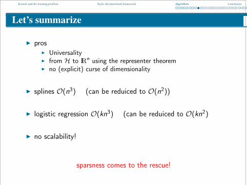
Let’s summarize
I prosI UniversalityI from H to IRn using the representer theoremI no (explicit) curse of dimensionality
I splines O(n3) (can be reduiced to O(n2))
I logistic regression O(kn3) (can be reduiced to O(kn2)
I no scalability!
sparsness comes to the rescue!
Kernels and the learning problem Tools: the functional framework Algorithms Conclusion
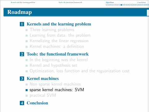
Roadmap
1 Kernels and the learning problemThree learning problemsLearning from data: the problemKernelizing the linear regressionKernel machines: a definition
2 Tools: the functional frameworkIn the beginning was the kenrelKernel and hypothesis setOptimization, loss function and the reguarization cost
3 Kernel machinesNon sparse kernel machinessparse kernel machines: SVMpractical SVM
4 Conclusion

Kernels and the learning problem Tools: the functional framework Algorithms Conclusion
SVM: the separable case (no noise)
maxf ,α0
m
with yi(f (xi ) + α0
)≥ m
and 12‖f ‖
2H = 1
⇔
{minf ,α0
12‖f ‖
2H
with yi(f (xi ) + α0
)≥ 1
3 ways to represent function f
f (x)︸ ︷︷ ︸in the RKHS H
=d∑
j=1
wj φj(x)︸ ︷︷ ︸d features
=n∑
i=1
αi yi k(x, xi )︸ ︷︷ ︸n data points
{minw,α0
12‖w‖
2IRd = 1
2 w>w
with yi(w>φ(xi ) + α0
)≥ 1
⇔
{minα,α0
12 α>Kα
with yi(α>K (:, i) + α0
)≥ 1

Kernels and the learning problem Tools: the functional framework Algorithms Conclusion
using relevant features...
a data point becomes a function x −→ k(x, .)

Kernels and the learning problem Tools: the functional framework Algorithms Conclusion
Representer theorem for SVM{
minf ,α0
12‖f ‖
2H
with yi(f (xi ) + α0
)≥ 1
LagrangianL(f , α0,α) =
12‖f ‖2H −
n∑i=1
αi(yi (f (xi ) + α0)− 1
)α ≥ 0
optimility condition: ∇f L(f , α0,α) = 0⇔ f (x) =n∑
i=1
αiyik(xi , x)
Eliminate f from L:
‖f ‖2H =
n∑i=1
n∑j=1
αiαjyiyjk(xi , xj)
n∑i=1
αiyi f (xi ) =n∑
i=1
n∑j=1
αiαjyiyjk(xi , xj)
Q(α0,α) = −12
n∑i=1
n∑j=1
αiαjyiyjk(xi , xj)−n∑
i=1
αi(yiα0 − 1
)
Kernels and the learning problem Tools: the functional framework Algorithms Conclusion
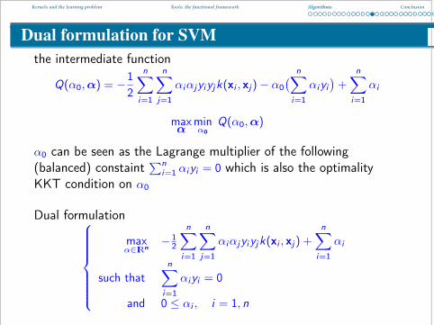
Dual formulation for SVMthe intermediate function
Q(α0,α) = −12
n∑i=1
n∑j=1
αiαjyiyjk(xi , xj)− α0( n∑
i=1
αiyi)
+n∑
i=1
αi
maxα
minα0
Q(α0,α)
α0 can be seen as the Lagrange multiplier of the following(balanced) constaint
∑ni=1 αiyi = 0 which is also the optimality
KKT condition on α0
Dual formulation
maxα∈IRn
− 12
n∑i=1
n∑j=1
αiαjyiyjk(xi , xj) +n∑
i=1
αi
such thatn∑
i=1
αiyi = 0
and 0 ≤ αi , i = 1, n
Kernels and the learning problem Tools: the functional framework Algorithms Conclusion
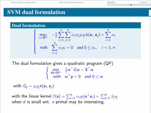
SVM dual formulation
Dual formulationmaxα∈IRn
− 12
n∑i=1
n∑j=1
αiαjyiyjk(xi , xj) +n∑
i=1
αi
withn∑
i=1
αiyi = 0 and 0 ≤ αi , i = 1, n
The dual formulation gives a quadratic program (QP){min
α∈IRn12α>Gα− 1I>α
with α>y = 0 and 0 ≤ α
with Gij = yiyjk(xi , xj)
with the linear kernel f (x) =∑n
i=1 αiyi (x>xi ) =∑d
j=1 βjxj
when d is small wrt. n primal may be interesting.
Kernels and the learning problem Tools: the functional framework Algorithms Conclusion
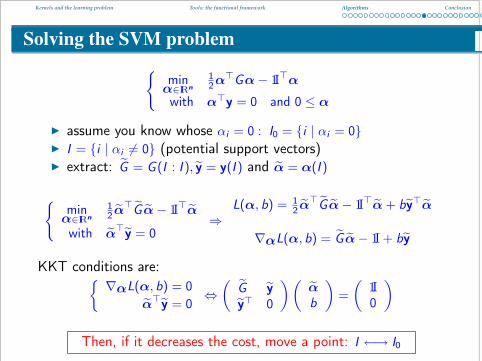
Solving the SVM problem{
minα∈IRn
12α>Gα− 1I>α
with α>y = 0 and 0 ≤ α
I assume you know whose αi = 0 : I0 = {i | αi = 0}I I = {i | αi 6= 0} (potential support vectors)I extract: G = G (I : I ), y = y(I ) and α = α(I )
{min
α∈IRn12 α>G α− 1I>α
with α>y = 0⇒
L(α, b) = 12 α>G α− 1I>α + by>α
∇αL(α, b) = G α− 1I + by
KKT conditions are:{∇αL(α, b) = 0
α>y = 0⇔(
G yy> 0
)(αb
)=
(1I0
)
Then, if it decreases the cost, move a point: I ←→ I0

Kernels and the learning problem Tools: the functional framework Algorithms Conclusion
The importance of being support
f (x) =n∑
i=1
αiyik(xi , x)
datapoint
αconstraint
valuexi useless αi = 0 yi
(f (xi ) + α0
)> 1
xi support αi > 0 yi(f (xi ) + α0
)= 1
Table: When a data point is « support » it lies exacty on the margin.
here lies the efficency of the algorithm (and its complexity)!
sparsness: αi = 0

Kernels and the learning problem Tools: the functional framework Algorithms Conclusion
Data groups: illustration
f (x) =n∑
i=1
αik(x, xi ) + α0
D(x) = sign(f (x)
)
useless data important data suspicious datawell classified support
α = 0 0 < α < C α = C
Kernels and the learning problem Tools: the functional framework Algorithms Conclusion
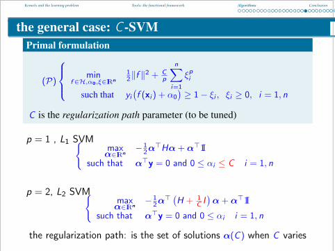
the general case: C -SVMPrimal formulation
(P)
minf∈H,α0,ξ∈IRn
12‖f ‖
2 + Cp
n∑i=1
ξpi
such that yi(f (xi ) + α0
)≥ 1− ξi , ξi ≥ 0, i = 1, n
C is the regularization path parameter (to be tuned)
p = 1 , L1 SVM{maxα∈IRn
− 12α>Hα + α>1I
such that α>y = 0 and 0 ≤ αi ≤ C i = 1, n
p = 2, L2 SVM{maxα∈IRn
− 12α>
(H + 1
C I)α + α>1I
such that α>y = 0 and 0 ≤ αi i = 1, n
the regularization path: is the set of solutions α(C ) when C varies

Kernels and the learning problem Tools: the functional framework Algorithms Conclusion
Two more ways to derivate SVM
Using the hinge loss
minf∈H,α0∈IR
1p
n∑i=1
max(0, 1− yi (f (xi ) + α0)
)p+
12C‖f ‖2
Minimizing the distance betwen the convex hulls
minα
‖u − v‖2Hwith u(x) =
∑{i|yi=1}
αik(xi , x), v(x) =∑
{i|yi=−1}
αik(xi , x)
and∑{i|yi=1}
αi = 1,∑
{i|yi=−1}
αi = 1, 0 ≤ αi i = 1, n
f (x) =2
‖u − v‖2H
(u(x)− v(x)
)and α0 =
‖u‖2H − ‖v‖2H‖u − v‖2H

Kernels and the learning problem Tools: the functional framework Algorithms Conclusion
Regularization path for SVM
minf∈H
n∑i=1
max(1− yi f (xi ), 0) +λ
2‖f ‖2H
Iα is the set of support vectors s.t. yi f (xi ) = 1;
∇f J(f ) =∑i∈Iα
αiyiK (xi , .) +∑i∈I1
yiK (xi , .) + λ f (.) with αi = ∂H(xi )
in particular at point xj ∈ Iα (fo(xj ) = fn(xj ) = yj)∑i∈Iα αioyiK (xi , xj) = −
∑i∈I1 yiK (xi , xj)− λo yj∑
i∈Iα αinyiK (xi , xj) = −∑
i∈I1 yiK (xi , xj)− λn yj
G (αn − αo) = (λo − λn)y avec Gij = yiK (xi , xj)
αn = αo + (λo − λn)ww = (G)−1y

Kernels and the learning problem Tools: the functional framework Algorithms Conclusion
Example of regularization path
α estimation and data selection

Kernels and the learning problem Tools: the functional framework Algorithms Conclusion
How to choose ` and P to get linear regularization path?
the path is piecewise linear ⇔ one is piecewise quadraticand the other is piecewise linear
the convex case [Rosset & Zhu, 07]
minβ∈IRd
`(β) + λP(β)
1. piecewise linearity: limε→0
β(λ+ ε)− β(λ)
ε= constant
2. optimality∇`(β(λ)) + λ∇P(β(λ)) = 0∇`(β(λ+ ε)) + (λ+ ε)∇P(β(λ+ ε)) = 0
3. Taylor expension
limε→0
β(λ+ ε)− β(λ)
ε=[∇2`(β(λ)) + λ∇2P(β(λ))
]−1∇P(β(λ))
∇2`(β(λ)) = constant and ∇2P(β(λ)) = 0

Kernels and the learning problem Tools: the functional framework Algorithms Conclusion
Problems with Piecewise linear regularization path
L P regression classification clusteringL2 L1 Lasso/LARS L1 L2 SVM PCA L1L1 L2 SVR SVM OC SVML1 L1 L1 LAD L1 SVM
Danzig Selector
Table: example of piecewise linear regularization path algorithms.
P : Lp =d∑
j=1
|βj |p L : Lp : |f (x)− y |p hinge (yf (x)− 1)p+
ε-insensitive
{0 if |f (x)− y | < ε|f (x)− y | − ε else
Huber’s loss:
{|f (x)− y |2 if |f (x)− y | < t2t|f (x)− y | − t2 else
Kernels and the learning problem Tools: the functional framework Algorithms Conclusion
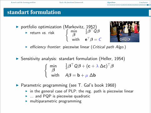
standart formulation
I portfolio optimization (Markovitz, 1952)I return vs. risk
{minβ
12β>Qβ
with e>β = C
I efficiency frontier: piecewise linear (Critical path Algo.)
I Sensitivity analysis: standart formulation (Heller, 1954){minβ
12β>Qβ + (c + λ ∆c)>β
with Aβ = b + µ ∆b
I Parametric programming (see T. Gal’s book 1968)I in the general case of PLP: the reg. path is piecewise linearI ... and PQP is piecewise quadraticI multiparametric programming

Kernels and the learning problem Tools: the functional framework Algorithms Conclusion
ν-SVM and other formulations...
ν ∈ [0, 1]
(ν)
min
f ,α0,ξ,m12‖f ‖
2H + 1
np
n∑i=1
ξpi − νm
with yi(f (xi ) + α0
)≥ m − ξi , i = 1, n,
and m ≥ 0, ξi ≥ 0, i = 1, n,
for p = 1 the dual formulation is:maxα∈IRn
− 12α>Gα
with α>y = 0 et 0 ≤ αi ≤ 1n i = 1, n
and ν ≤ α>1I
C = 1m

Kernels and the learning problem Tools: the functional framework Algorithms Conclusion
SVM with non symetric costs
problem in the primal minf∈H,α0,ξ∈IRn
12‖f ‖
2H + C+
∑{i|yi=1}
ξpi + C−∑
{i|yi=−1}
ξpi
with yi(f (xi ) + α0
)≥ 1− ξi , ξi ≥ 0, i = 1, n
for p = 1 the dual formulation is the following:{maxα∈IRn
− 12α>Gα + α>1I
with α>y = 0 and 0 ≤ αi ≤ C+ or C− i = 1, n

Kernels and the learning problem Tools: the functional framework Algorithms Conclusion
Generalized SVM
minf∈H,α0∈IR
n∑i=1
max(0, 1− yi (f (xi ) + α0)
)+
1Cϕ(f ) ϕ convex
in particular ϕ(f ) = ‖f ‖pp with p = 1 leads to L1 SVM.min
α∈IRn,α0,ξ1I>β + C1I>ξ
with yi( n∑
j=1
αjk(xi , xj) + α0)≥ 1− ξi ,
and −βi ≤ αi ≤ βi , ξi ≥ 0, i = 1, n
with β = |α|. the dual is:max
γ,δ,δ∗∈IR3n1I>γ
with y>γ = 0, δi + δ∗i = 1∑nj=1 γjk(xi , xj) = δi − δ∗i , i = 1, n
and 0 ≤ δi , 0 ≤ δ∗i , 0 ≤ γi ≤ C , i = 1, n
Mangassarian, 2001

Kernels and the learning problem Tools: the functional framework Algorithms Conclusion
SVM reduction (reduced set method))
I objective: compile the model
I f (x) =ns∑i=1
αik(xi , x), ns � n, ns too big
I compiled model as the solution of:
g(x) =nc∑i=1
βik(zi , x), nc � ns
I β, zi and c are tuned by minimizing:
minβ,zi‖g − f ‖2H
where
minβ,zi‖g − f ‖2H = α>Kxα + β>Kzβ − 2α>Kxzβ
some authors advice 0, 03 ≤ ncns≤ 0, 1
I solve it by using use (stochastic) gradient (its a RBF problem)Burges 1996, Ozuna 1997, Romdhani 2001
Kernels and the learning problem Tools: the functional framework Algorithms Conclusion
SVM and probabilities (1/2)
logIP(Y = 1|x)
IP(Y = −1|x)as (almost) the same sign as f (x)
logIP(Y = 1|x)
IP(Y = −1|x)= a1f (x) + a2 IP(Y = 1|x) = 1− 1
1 + expa1f (x)+a2
a1 et a2 estimated using maximum likelihoodsome facts
I SVM is universaly consistent (coverges towards the Bayes risk)I SVM asymptotically implements the bayes ruleI but theoreticaly: no consistency towards conditional
probabilities (due to the nature of sparsity)I to estimate conditional probabilities on an interval
(typicaly[ 12 − η,
12 + η]) to spasness in this interval (all data
points have to be support vectors)Platt, 99 ; Bartlett & Tewari, JMLR, 07
Kernels and the learning problem Tools: the functional framework Algorithms Conclusion
SVM and probabilities (2/2)
An alternative approach
g(x)− ε−(x) ≤ IP(Y = 1|x) ≤ g(x) + ε+(x)
with g(x) = 11+4−f (x)−α0
non parametric functions ε− and ε+ have to verify:
g(x) + ε+(x) = exp−a1(1−f (x)−α0)++a2
1− g(x)− ε−(x) = exp−a1(1+f (x)+α0)++a2
with a1 = log 2 and a2 = 0
Grandvalet et al., 07
Kernels and the learning problem Tools: the functional framework Algorithms Conclusion
logistic regression and the import vector machine
I Logistic regression is NON sparseI kernalize it using the dictionary strategyI Algorithm:
I find the solution of the KLR using only a subset S of the dataI build S iteratively using active constraint approach
I this trick brings sparsityI it estimates probabilityI it can naturally be generalized to the multiclass case
I efficent when uses:I a few import vectorsI component-wise update procedure
I extention using L1 KLRZhu & Hastie, 01 ; Keerthi et. al., 02

Kernels and the learning problem Tools: the functional framework Algorithms Conclusion
Multiclass SVMI one vs all: winner takes allI one vs one:
I max-wins votingI pairwise coupling: use probability
I global approach (size c × n),I formal (differents variations)
minf∈H,α0,ξ∈IRn
12
c∑`=1
‖f`‖2H +Cp
n∑i=1
c∑`=1, 6=yi
ξpi`
with yi(fyi (xi ) + byi − f`(xi )− b`
)≥ 1− ξi`
and ξi` ≥ 0 for i = 1, ..., n; ` = 1, ..., c ; ` 6= yi
non consistent estimator but practicaly usefullI structured outputs
approachproblemsize
number ofsub problems
all together n × c 11 vs. all n c1 vs. 1 2n
cc(c−1)
2Duan & Keerti, 05 ; Bartlett 06

Kernels and the learning problem Tools: the functional framework Algorithms Conclusion
Multiclass SVMI one vs all: winner takes allI one vs one:
I max-wins votingI pairwise coupling: use probability – best results
I global approach (size c × n),I formal (differents variations)
minf∈H,α0,ξ∈IRn
12
c∑`=1
‖f`‖2H +Cp
n∑i=1
c∑`=1, 6=yi
ξpi`
with yi(fyi (xi ) + byi − f`(xi )− b`
)≥ 1− ξi`
and ξi` ≥ 0 for i = 1, ..., n; ` = 1, ..., c ; ` 6= yi
non consistent estimator but practicaly usefullI structured outputs
approachproblemsize
number ofsub problems
all together n × c 11 vs. all n c1 vs. 1 2n
cc(c−1)
2Duan & Keerti, 05 ; Bartlett 06

Kernels and the learning problem Tools: the functional framework Algorithms Conclusion
Roadmap
1 Kernels and the learning problemThree learning problemsLearning from data: the problemKernelizing the linear regressionKernel machines: a definition
2 Tools: the functional frameworkIn the beginning was the kenrelKernel and hypothesis setOptimization, loss function and the reguarization cost
3 Kernel machinesNon sparse kernel machinessparse kernel machines: SVMpractical SVM
4 Conclusion
Kernels and the learning problem Tools: the functional framework Algorithms Conclusion
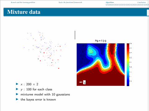
Mixture data
I x : 200 × 2I y : 100 for each classI mixturee model with 10 gaussiansI the bayes error is known
Kernels and the learning problem Tools: the functional framework Algorithms Conclusion
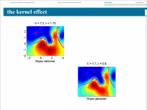
the kernel effect

Kernels and the learning problem Tools: the functional framework Algorithms Conclusion
tuning C and σ : grid search
for σ = 0.5 : 0.25 : 2
for C = 0.1 à 10000
3 different error estimate
Kernels and the learning problem Tools: the functional framework Algorithms Conclusion
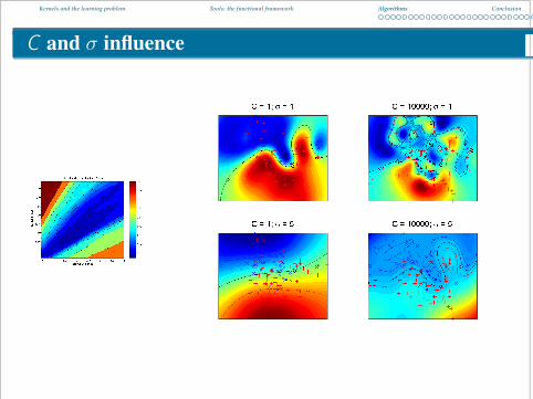
C and σ influence

Kernels and the learning problem Tools: the functional framework Algorithms Conclusion
checker board
I 2 classesI 500 examplesI separable

Kernels and the learning problem Tools: the functional framework Algorithms Conclusion
a separable case
n = 500 data points
n = 5000 data points

Kernels and the learning problem Tools: the functional framework Algorithms Conclusion
tuning C and σ : grid search
Kernels and the learning problem Tools: the functional framework Algorithms Conclusion
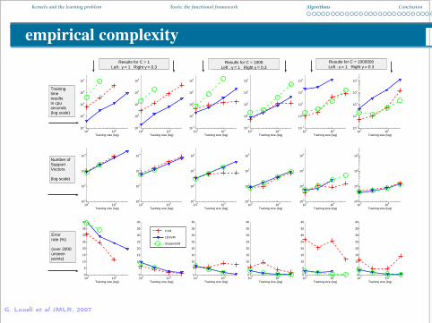
empirical complexity
103
104
10−1
100
101
102
103
Training size (log)
103
104
101
102
103
104
Training size (log)
103
104
0
5
10
15
20
25
30
35
40
Training size (log)
103
104
10−1
100
101
102
103
Training size (log)
103
104
101
102
103
104
Training size (log)
103
104
0
5
10
15
20
25
30
35
40
Training size (log)
103
104
10−1
100
101
102
103
Training size (log)
103
104
101
102
103
104
Training size (log)
103
104
0
5
10
15
20
25
30
35
40
Training size (log)
103
104
10−1
100
101
102
103
Training size (log)
103
104
101
102
103
104
Training size (log)
103
104
0
5
10
15
20
25
30
35
40
Training size (log)
103
104
10−1
100
101
102
103
Training size (log)
103
104
101
102
103
104
Training size (log)
103
104
0
5
10
15
20
25
30
35
40
Training size (log)
103
104
10−1
100
101
102
103
Training size (log)
103
104
101
102
103
104
Training size (log)
103
104
0
5
10
15
20
25
30
35
40
Training size (log)
CVM
LibSVM
SimpleSVM
Results for C = 1Left : γ = 1 Right γ = 0.3
Results for C = 1000Left : γ = 1 Right γ = 0.3
Results for C = 1000000Left : γ = 1 Right γ = 0.3
Trainingtimeresultsin cpuseconds(log scale)
Number ofSupportVectors
(log scale)
Errorrate (%)
(over 2000unseenpoints)
G. Loosli et al JMLR, 2007

Kernels and the learning problem Tools: the functional framework Algorithms Conclusion
ConclusionI nonlinearity throught kernel: using examples influenceI universality: kernel to functions (R.K.H.S.)I representer theorem: from functions to vectorsI L1 provides sparsity
a question of vocabulary
I margin: regularizationI Mercer kenrel: positive kernelI SVM: a method among others
I kernels (RKHS) universalityI regularization univ. consistencyI convexity efficiencyI sparsity efficiency
no (explicit) model
but a kernel, a cost and a regularity

Kernels and the learning problem Tools: the functional framework Algorithms Conclusion
Historical perspective on kernel machines
statistics
1960 Parzen, Nadaraya Watson
1970 Splines
1980 Kernels: Silverman, Hardle...
1990 sparsity: Donoho (pursuit),Tibshirani (Lasso)...
Statistical learning
1985 Neural networks:I non linear - universalI structural complexityI non convex optimization
1992 Vapnik et. al.I theory - regularization -
consistancyI convexity - LinearityI Kernel - universalityI sparsityI results: MNIST

Kernels and the learning problem Tools: the functional framework Algorithms Conclusion
what’s new since 1995
I ApplicationsI kernlisation w>x→ 〈f , k(x, .)〉HI kernel engineeringI sturtured outputsI applications: image, text, signal, bio-info...
I OptimizationI dual: mloss.orgI regularization pathI approximationI primal
I StatisticI proofs and boundsI model selection
I span boundI multikernel: tuning (k and σ)

Kernels and the learning problem Tools: the functional framework Algorithms Conclusion
challenges: towards tough learning
I the size effectI ready to use: automatizationI adaptative: on line context awareI beyond kenrels
I Automatic and adaptive model selectionI variable selectionI kernel tuning (k et σ)I hyperparametres: C , duality gap, λ
I IP change
I TheoryI non positive kernelsI a more general representer theorem

Kernels and the learning problem Tools: the functional framework Algorithms Conclusion
biblio: kernel-machines.orgI John Shawe-Taylor and Nello Cristianini Kernel Methods for Pattern Analysis,
Cambridge University Press, 2004I Bernhard Schölkopf and Alex Smola. Learning with Kernels. MIT Press,
Cambridge, MA, 2002.I Trevor Hastie, Robert Tibshirani and Jerome Friedman, The Elements of
Statistical Learning:. Data Mining, Inference, and Prediction, springer, 2001
I Léon Bottou, Olivier Chapelle, Dennis DeCoste and Jason Weston Large-ScaleKernel Machines (Neural Information Processing, MIT press 2007
I Olivier Chapelle, Bernhard Scholkopf and Alexander Zien, Semi-supervisedLearning, MIT press 2006
I Vladimir Vapnik. Estimation of Dependences Based on Empirical Data.Springer Verlag, 2006, 2nd edition.
I Vladimir Vapnik. The Nature of Statistical Learning Theory. Springer, 1995.
I Grace Wahba. Spline Models for Observational Data. SIAM CBMS-NSFRegional Conference Series in Applied Mathematics vol. 59, Philadelphia, 1990
I Alain Berlinet and Christine Thomas-Agnan, Reproducing Kernel Hilbert Spacesin Probability and Statistics,Kluwer Academic Publishers, 2003
I Marc Atteia et Jean Gaches , Approximation Hilbertienne - Splines, Ondelettes,Fractales, PUG, 1999