Mach Learn (2012) 86:335–367DOI 10.1007/s10994-011-5266-3

Statistical analysis of kernel-based least-squaresdensity-ratio estimation

Takafumi Kanamori · Taiji Suzuki · Masashi Sugiyama

Received: 8 April 2009 / Accepted: 30 September 2011 / Published online: 1 November 2011© The Author(s) 2011

Abstract The ratio of two probability densities can be used for solving various machinelearning tasks such as covariate shift adaptation (importance sampling), outlier detection(likelihood-ratio test), feature selection (mutual information), and conditional probabilityestimation. Several methods of directly estimating the density ratio have recently been de-veloped, e.g., moment matching estimation, maximum-likelihood density-ratio estimation,and least-squares density-ratio fitting. In this paper, we propose a kernelized variant of theleast-squares method for density-ratio estimation, which is called kernel unconstrained least-squares importance fitting (KuLSIF). We investigate its fundamental statistical propertiesincluding a non-parametric convergence rate, an analytic-form solution, and a leave-one-out cross-validation score. We further study its relation to other kernel-based density-ratioestimators. In experiments, we numerically compare various kernel-based density-ratio es-timation methods, and show that KuLSIF compares favorably with other approaches.

Keywords Density ratio · Kernel method · Least-square method · Statistical consistency

1 Introduction

The problem of estimating the ratio of two probability densities is attracting a great dealof attention these days, since the density ratio can be used for various purposes (Sugiyamaet al. 2009; Sugiyama et al. 2012), such as covariate shift adaptation (Shimodaira 2000;

Editor: Massimiliano Pontil

T. Kanamori (�)Nagoya University, Nagoya, Japane-mail: kanamori@is.nagoya-u.ac.jp

T. SuzukiUniversity of Tokyo, Tokyo, Japane-mail: s-taiji@stat.t.u-tokyo.ac.jp

M. SugiyamaTokyo Institute of Technology, Tokyo, Japane-mail: sugi@cs.titech.ac.jp

336 Mach Learn (2012) 86:335–367

Zadrozny 2004; Sugiyama and Müller 2005; Huang et al. 2007; Sugiyama et al. 2007;Bickel et al. 2009; Quiñonero-Candela et al. 2009; Sugiyama and Kawanabe 2011), outlierdetection (Hido et al. 2008, 2011; Smola et al. 2009; Kawahar and Sugiyama 2011), diver-gence estimation (Nguyen et al. 2010; Suzuki et al. 2008, 2009), and conditional probabilityestimation (Sugiyama et al. 2010; Sugiyama 2010).

A naive approach to density-ratio estimation is to first separately estimate two probabil-ity densities (corresponding to the numerator and the denominator of the ratio), and thentake the ratio of the estimated densities. However, density estimation is known to be a hardproblem particularly in high-dimensional cases unless we have simple and good parametricdensity models (Vapnik 1998; Härdle et al. 2004; Kanamori et al. 2010), which may not bethe case in practice.

For reliable statistical inference, it is important to develop methods of directly estimatingthe density ratio without going through density estimation. In the context of case-controlstudies, Qin (1998) has proposed a direct method of estimating the density ratio by match-ing moments of the two distributions. Another density-ratio estimation approach uses theM-estimator (Nguyen et al. 2010) based on non-asymptotic variational characterization ofthe f -divergence (Ali and Silvey 1966; Csiszár 1967). See also Sugiyama et al. (2008a)for a similar algorithm using the Kullback-Leibler divergence. Kanamori et al. (2009) havedeveloped a squared-loss version of the M-estimator for linear density-ratio models calledunconstrained Least-Squares Importance Fitting (uLSIF), and have shown that uLSIF pos-sesses superior computational properties. That is, a closed-form solution is available and theleave-one-out cross-validation score can be analytically computed. As another approach, onecan use logistic regression for the inference of density ratios, since the ratio of two prob-ability densities is directly connected to the posterior probability of labels in classificationproblems. Using the Bayes formula, the estimated posterior probability can be transformedto an estimator of density ratios (Bickel et al. 2007).

Various kernel-based approaches are also available for density-ratio estimation. Thekernel mean matching (KMM) method (Gretton et al. 2009) directly gives estimates ofthe density ratio by matching the two distributions using universal reproducing kernelHilbert spaces (Steinwart 2001). KMM can be regarded as a kernelized variant of Qin’smoment matching estimator (Qin 1998). Nguyen’s approach based on the M-estimator(Nguyen et al. 2010) also has a kernelized variant. Non-parametric convergence proper-ties of the M-estimator in reproducing kernel Hilbert spaces have been elucidated underthe Kullback-Leibler divergence (Nguyen et al. 2010; Sugiyama et al. 2008b). For thedensity-ratio estimation, one can also apply kernel logistic regression (Wahba et al. 1993;Zhu and Hastie 2001), instead of conventional linear logistic models for the inference of theposterior distribution in classification problems.

In this paper, we first propose a kernelized variant of uLSIF (called KuLSIF), and showthat the solution of KuLSIF as well as its leave-out-out cross-validation score can be com-puted analytically, as the original uLSIF for linear models. We then elucidate the statisti-cal consistency and convergence rate of KuLSIF based on the argument on non-parametricbounds (van de Geer 2000; Nguyen et al. 2010). We further study the relation betweenKuLSIF and other kernel-based density-ratio estimators. Finally, statistical performance ofKuLSIF is numerically compared with other kernel-based density-ratio estimators in exper-iments.

The rest of this paper is organized as follows. In Sect. 2, we formulate the problem ofdensity-ratio estimation and briefly review the existing least-squares method. In Sect. 3,we describe the kernelized variant of uLSIF, and show its statistical properties such as theconvergence rate and availability of the analytic-form solution and the analytic-form leave-one-out cross-validation score. In Sect. 4, we investigate the relation between KuLSIF and

Mach Learn (2012) 86:335–367 337

other kernel-based density-ratio estimators. In Sect. 5, we experimentally investigate com-putational efficiency and statistical performance of KuLSIF. Finally, in Sect. 6, we concludeby summarizing our contributions and showing possible future directions. Detailed proofsand calculations are deferred to Appendix. In a companion paper (Kanamori et al. 2011),computational properties of the KuLSIF method are further investigated from the viewpointof condition numbers.

2 Estimation of density ratios

In this section, we formulate the problem of density-ratio estimation and briefly review theleast-squares density-ratio estimator.

2.1 Formulation and notations

Consider two probability distributions P and Q on a probability space Z . Assume thatthe distributions P and Q have the probability densities p and q , respectively. We assumep(x) > 0 for all x ∈ Z . Suppose that we are given two sets of independent and identicallydistributed (i.i.d.) samples,

X1, . . . ,Xn

i.i.d.∼ P, Y1, . . . , Ym

i.i.d.∼ Q. (1)

Our goal is to estimate the density ratio

w0(x) = q(x)

p(x)(≥ 0)

based on the observed samples.We summarize some notations to be used throughout the paper. For two integers n and

m, n ∧ m denotes min{m,n}. For a vector a in the Euclidean space, ‖a‖ denotes the Eu-clidean norm. Given a probability distribution P and a random variable h(X), we denotethe expectation of h(X) under P by

∫hdP or

∫h(x)P (dx). Let ‖ · ‖∞ be the infinity norm,

and ‖ · ‖P be the L2-norm under the probability P , i.e., ‖h‖2P = ∫ |h|2dP . For a reproducing

kernel Hilbert space (RKHS) H (Aronszajn 1950), the inner product and the norm on H aredenoted as 〈·, ·〉H and ‖ · ‖H , respectively.

Below we review the least-squares approach to density-ratio estimation proposed byKanamori et al. (2009).

2.2 Least-squares approach

The linear model

w(x) =B∑

i=1

αihi(x) (2)

is assumed for the estimation of the density ratio w0, where the coefficients α1, . . . , αB arethe parameters of the model. The basis functions hi, i = 1, . . . ,B are chosen so that thenon-negativity condition hi(x) ≥ 0 is satisfied. A practical choice would be the Gaussiankernel function hi(x) = e−‖x−ci‖2/2σ 2

with appropriate kernel center ci ∈ Z and kernel widthσ (Sugiyama et al. 2008a).

338 Mach Learn (2012) 86:335–367

The unconstrained least-squares importance fitting (uLSIF) (Kanamori et al. 2009) esti-mates the parameter α based on the squared error:

1

2

∫(w − w0)

2dP =1

2

∫w2dP −

∫wdQ + 1

2

∫w2

0dP.

The last term in the above expression is a constant and can be safely ignored when minimiz-ing the squared error of the estimator w. Therefore, the solution of the following minimiza-tion problem over the linear model (2),

minw

1

2n

n∑

i=1

(w(Xi))2 − 1

m

m∑

j=1

w(Yj ) + λ · Reg(α), (3)

is expected to approximate the true density-ratio w0, where the regularization term Reg(α)

with the regularization parameter λ is introduced to avoid overfitting. Let α be the op-timal solution of (3) under the linear model (2). Then the estimator of w0 is given asw(x) = ∑B

i=1 αihi(x). There are several ways to impose the non-negativity conditionw(x) ≥ 0 (Kanamori et al. 2009). Here, truncation of w defined as

w+(x) = max{w(x), 0}is used to ensure the non-negativity of the estimator.

It is worthwhile to point out that uLSIF can be regarded as an example of the M-estimator(Nguyen et al. 2010) with the quadratic loss function, i.e., φ∗(f ) = f 2/2 in Nguyen’s nota-tion. Nguyen’s M-estimator is constructed based on the f -divergence from Q and P . Due tothe asymmetry of f -divergence, the estimation error evaluated with respect to P rather thanQ is obtained in uLSIF. uLSIF has an advantage in computation over other M-estimators:When Reg(α) = ‖α‖2/2, the estimator α can be obtained in an analytic form. As a result,the leave-one-out cross-validation (LOOCV) score can also be computed in a closed form(Kanamori et al. 2009), which allows us to compute the LOOCV score very efficiently.LOOCV is an (almost) unbiased estimator of the prediction error and can be used for de-termining hyper-parameters such as the regularization parameter and the Gaussian kernelwidth. In addition, for the L1-regularization Reg(α) = ∑B

i=1 |αi |, Kanamori et al. (2009)applied the path-following algorithm to regularization parameter estimation, which highlycontributes to reducing the computational cost in the model selection phase.

3 Kernel uLSIF

The purpose of this paper is to show that a kernelized variant of uLSIF (which we refer to askernel uLSIF; KuLSIF) has good theoretical properties and thus useful. In this section, weformalize the KuLSIF algorithm and show its fundamental statistical properties.

3.1 uLSIF on RKHS

We assume that the model for the density ratio is an RKHS H endowed with a kernel func-tion k on Z × Z , and we consider the optimization problem (3) on H. Then, the estimatorw is obtained as an optimal solution of

minw

1

2n

n∑

i=1

(w(Xi))2 − 1

m

m∑

j=1

w(Yj ) + λ

2‖w‖2

H s.t. w ∈ H, (4)

Mach Learn (2012) 86:335–367 339

where the regularization term λ2 ‖w‖2

H with the regularization parameter λ (≥ 0) is intro-duced to avoid overfitting. We may also consider the truncated estimator w+ = max{w,0}.The estimator based on the loss function (4) is called KuLSIF.

The computation of KuLSIF is efficiently conducted. For infinite-dimensional H, theproblem (4) is an infinite-dimensional optimization problem. The representer theorem(Kimeldorf and Wahba 1971), however, is applicable to RKHSs, which allows us to trans-form the infinite-dimensional optimization problem to a finite-dimensional one. Let K11,K12, and K21 be the sub-matrices of the Gram matrix:

(K11)ii′ =k(Xi,Xi′), (K12)ij = k(Xi, Yj ), K21 = K�12,

where i, i ′ = 1, . . . , n, j, j ′ = 1, . . . ,m. Then, detailed analysis leads us to the specific formof the solution as follows.

Theorem 1 (Analytic solution of KuLSIF) Suppose λ > 0. Then, the KuLSIF estimator isgiven as

w(z) =n∑

i=1

αik(z,Xi) + 1

mλ

m∑

j=1

k(z,Yj ).

The coefficients α = (α1, . . . , αn)� are given by the solution of the linear equation

(1

nK11 + λIn

)

α = − 1

nmλK121m, (5)

where In is the n by n identity matrix and 1m is the column vector defined as 1m =(1, . . . ,1)� ∈ m.

The proof is deferred to Appendix A. Theorem 1 implies that it is sufficient to find n vari-ables α1, . . . , αn to obtain the estimator w and that the estimator has the analytic-form solu-tion.

Theorem 1 also guarantees that the parameters in the KuLSIF estimator are obtained bythe solution of the following optimization problem:

minα

1

2α�

(1

nK11 + λIn

)

α + 1

nmλ1�

mK21α, α ∈ n, (6)

where we used the fact that the solution of Ax = b is given as the minimizer of 12x�Ax −

b�x, when A is positive-semidefinite. When the sample size of n is large, numerically op-timizing the quadratic function in (6) can be computationally more efficient than directlysolving the linear equation (5). In Sect. 5, numerical experiments are carried out to investi-gate the computational efficiency of KuLSIF.

3.2 Leave-one-out cross-validation

The leave-one-out cross-validation (LOOCV) score for the KuLSIF estimator can also beobtained analytically as well as the coefficient parameters of the kernel model. Let us mea-sure the accuracy of the KuLSIF estimator, w+ = max{w,0}, by

1

2

∫w2

+dP −∫

w+dQ,

340 Mach Learn (2012) 86:335–367

which is equal to the squared error of w+ up to a constant term. Then the LOOCV score ofw+ under the squared error is defined as

LOOCV = 1

n ∧ m

n∧m∑

�=1

{1

2(w

(�)+ (x�))

2 − w(�)+ (y�)

}

, (7)

where w(�)+ = max{w(�),0} is the estimator based on training samples except1 x� and y�. The

hyper-parameters achieving the minimum value of LOOCV are chosen.Thanks to the analytic-form solution shown in Theorem 1, the leave-one-out solution

w(�) can be computed efficiently from w by the use of the Sherman-Woodbury-Morrisonformula (Golub and Loan 1996). Details of the analytic LOOCV expression are presentedin Appendix B.

3.3 Statistical consistency of KuLSIF

The following theorem reveals the convergence rate of the KuLSIF estimator.

Theorem 2 (Convergence rate of KuLSIF) Let Z be a probability space, and H be theRKHS endowed with the kernel function k defined on Z × Z . Suppose that supx∈Z k(x, x) <

∞, and that the bracketing entropy HB(δ, HM,P ) is bounded above by O(M/δ)γ , whereγ is a constant satisfying 0 < γ < 2 (see Appendix C for the detailed definition). Set theregularization parameter λ = λn,m so that2

limn,m→∞λn,m = 0, λ−1

n,m = O((n ∧ m)1−δ) (n,m → ∞),

where n ∧ m = min{n,m} and δ is an arbitrary number satisfying 1 − 2/(2 + γ ) < δ < 1.Then, for q/p = w0 ∈ H, we have

‖w+ − w0‖P ≤ ‖w − w0‖P = Op(λ1/2n,m),

where ‖ · ‖P is the L2-norm under the probability P .

The proof is available in Appendix C. See Nguyen et al. (2010) and Sugiyama et al.(2008b) for similar convergence analysis for the logarithmic loss function. The conditionlimn,m→∞ λn,m = 0 means that the regularization parameter λn,m should vanish asymptoti-cally, but the condition λ−1

n,m = O((n ∧ m)1−δ) means that the regularization parameter λn,m

should not vanish too fast. As shown in the proof of the theorem, the assumption w0 ∈ Himposes supx∈Z w0(x) ≤ ‖w0‖H supx∈Z

√k(x, x) < ∞. For example, the ratio of two Gaus-

sian distributions with different means or variances does not satisfy this condition (see Ya-mada et al. 2011 for how to handle such a situation).

1The index of removed samples can be different for x and y, i.e., x�1 and y�2 (�1 �= �2) can be removed. Forthe sake of simplicity, however, we suppose that the samples x� and y� are removed in the computation ofLOOCV.2The multivariate big-O notation f (n,m) = O(g(n,m)), (n,m → ∞) implies that there exist C > 0, n0 > 0,and m0 > 0 such that the inequality |f (n,m)| ≤ C|g(n,m)| holds for all n > n0 and all m > m0.

Mach Learn (2012) 86:335–367 341

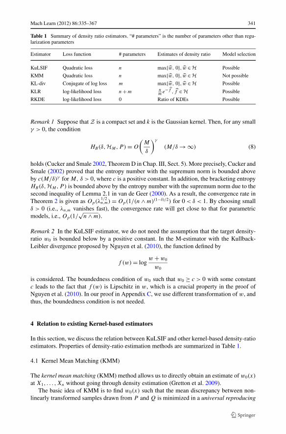
Table 1 Summary of density ratio estimators. “# parameters” is the number of parameters other than regu-larization parameters

Estimator Loss function # parameters Estimates of density ratio Model selection

KuLSIF Quadratic loss n max{w, 0}, w ∈ H Possible

KMM Quadratic loss n max{w, 0}, w ∈ H Not possible

KL-div Conjugate of log loss m max{w, 0}, w ∈ H Possible

KLR log-likelihood loss n + m nme−f , f ∈ H Possible

RKDE log-likelihood loss 0 Ratio of KDEs Possible

Remark 1 Suppose that Z is a compact set and k is the Gaussian kernel. Then, for any smallγ > 0, the condition

HB(δ, HM,P ) = O

(M

δ

)γ

(M/δ → ∞) (8)

holds (Cucker and Smale 2002, Theorem D in Chap. III, Sect. 5). More precisely, Cucker andSmale (2002) proved that the entropy number with the supremum norm is bounded aboveby c(M/δ)γ for M, δ > 0, where c is a positive constant. In addition, the bracketing entropyHB(δ, HM,P ) is bounded above by the entropy number with the supremum norm due to thesecond inequality of Lemma 2.1 in van de Geer (2000). As a result, the convergence rate inTheorem 2 is given as Op(λ

1/2n,m) = Op(1/(n ∧ m)(1−δ)/2) for 0 < δ < 1. By choosing small

δ > 0 (i.e., λn,m vanishes fast), the convergence rate will get close to that for parametricmodels, i.e., Op(1/

√n ∧ m).

Remark 2 In the KuLSIF estimator, we do not need the assumption that the target density-ratio w0 is bounded below by a positive constant. In the M-estimator with the Kullback-Leibler divergence proposed by Nguyen et al. (2010), the function defined by

f (w) = logw + w0

w0

is considered. The boundedness condition of w0 such that w0 ≥ c > 0 with some constantc leads to the fact that f (w) is Lipschitz in w, which is a crucial property in the proof ofNguyen et al. (2010). In our proof in Appendix C, we use different transformation of w, andthus, the boundedness condition is not needed.

4 Relation to existing Kernel-based estimators

In this section, we discuss the relation between KuLSIF and other kernel-based density-ratioestimators. Properties of density-ratio estimation methods are summarized in Table 1.

4.1 Kernel Mean Matching (KMM)

The kernel mean matching (KMM) method allows us to directly obtain an estimate of w0(x)

at X1, . . . ,Xn without going through density estimation (Gretton et al. 2009).The basic idea of KMM is to find w0(x) such that the mean discrepancy between non-

linearly transformed samples drawn from P and Q is minimized in a universal reproducing

342 Mach Learn (2012) 86:335–367

kernel Hilbert space (Steinwart 2001). We introduce the definition of universal kernels be-low.

Definition 1 (Definition 4.52 in Steinwart 2001) A continuous kernel k on a compact metricspace Z is called universal if the RKHS H of k is dense in the set of all continuous functionson Z , that is, for every continuous function g on Z and all ε > 0, there exists an f ∈ H suchthat ‖f − g‖∞ < ε. The corresponding RKHS is called a universal RKHS.

The Gaussian kernel on a compact set Z is an example of universal kernels. Let H be auniversal RKHS endowed with a universal kernel function k : Z × Z → . Then, one caninfer the density ratio w0 by solving the following minimization problem:

minw

1

2

∥∥∥∥

∫w(x)k(·, x)P (dx) −

∫k(·, y)Q(dy)

∥∥∥∥

2

H,

s.t.∫

w dP = 1 and w ≥ 0.

(9)

Huang et al. (2007) proved that the solution of (9) is given as w = w0, when Q is absolutelycontinuous with respect to P .

An empirical version of the above problem is reduced to the following convex quadraticprogram:

minw1,...,wn

1

2n

n∑

i,j=1

wiwjk(Xi,Xj ) − 1

m

m∑

j=1

n∑

i=1

wik(Xi, Yj ),

s.t.

∣∣∣∣1

n

n∑

i=1

wi − 1

∣∣∣∣ ≤ ε and 0 ≤ w1,w2, . . . ,wn ≤ B.

(10)

The tuning parameters, B ≥ 0 and ε ≥ 0, control the regularization effects. The opti-mal solution (w1, . . . , wn) is an estimate of the density ratio at the samples from P , i.e.,w0(X1), . . . ,w0(Xn). KMM does not estimate the function w0 on Z but the values on sam-ple points, while the assumption that w0 ∈ H is not required.

We study the relation between KuLSIF and KMM. Below, we assume that the truedensity-ratio w0 = q/p is included in the RKHS H. Let �(w) be

�(w) =∫

k(·, x)w(x)P (dx) −∫

k(·, y)Q(dy). (11)

Then the loss function of KMM on H under the population distribution is written as

LKMM(w) = 1

2‖�(w)‖2

H.

In the estimation phase, an empirical approximation of LKMM is optimized in the KMMalgorithm. On the other hand, the (unregularized) loss function of KuLSIF is given by

LKuLSIF(w) = 1

2

∫w2dP −

∫wdQ.

Both LKMM and LKuLSIF are minimized at the true density-ratio w0 ∈ H. Although somelinear constraints may be introduced in the optimization phase, we study the optimization

Mach Learn (2012) 86:335–367 343

problems of LKMM and LKuLSIF without constraints. This is because when the sample sizetends to infinity, the optimal solutions of LKMM and LKuLSIF without constraints automati-cally satisfy the required constraints such as

∫wdP = 1 and w ≥ 0.

We consider the extremal condition of LKuLSIF(w) at w0. Substituting

w = w0 + δ · v (δ ∈ , v ∈ H)

into LKuLSIF(w), we have

LKuLSIF(w0 + δv) − LKuLSIF(w0) = δ

{∫w0vdP −

∫vdQ

}

+ δ2

2

∫v2dP.

Since LKuLSIF(w0 + δv) is minimized at δ = 0, the derivative of LKuLSIF(w0 + δv) at δ = 0vanishes, i.e.,

∫w0vdP −

∫vdQ = 0. (12)

The equality (12) holds for arbitrary v ∈ H. Using the reproducing property of the kernelfunction k, we can derive another expression of (12) as follows

∫w0vdP −

∫vdQ =

∫w0(x)〈k(·, x), v〉HP (dx) −

∫〈k(·, y), v〉HQ(dy)

=⟨∫

k(·, x)w0(x)P (dx) −∫

k(·, y)Q(dy), v

⟩

H

= ⟨�(w0), v

⟩H = 0, ∀v ∈ H. (13)

Rigorous proof of the above formula is shown in Appendix D. As a result, we obtain�(w0) = 0. The above expression implies that �(w) is the Gâteaux derivative (Zeidler1986, Sect. 4.2) of LKuLSIF at w ∈ H, that is,

d

dδLKuLSIF(w + δ · v)

∣∣∣∣δ=0

= 〈�(w), v〉H (14)

holds for all v ∈ H. Let DLKuLSIF be the Gâteaux derivative of LKuLSIF over the RKHS H.Then we have DLKuLSIF = �, and the equality

LKMM(w) = 1

2‖DLKuLSIF(w)‖2

H (15)

holds. Tsuboi et al. (2008) have pointed out a similar relation for the M-estimator based onthe Kullback-Leibler divergence.

Now we give an interpretation of (15) through an analogous optimization example in theEuclidean space. Let f : d → be a differentiable function, and consider the optimizationproblem minx f (x). At an optimal solution x0, the extremal condition ∇f (x0) = 0 shouldhold, where ∇f is the gradient of f with respect to x. Thus, instead of minimizing f , min-imization of ‖∇f (x)‖2 also provides the minimizer of f . This corresponds to the relationbetween KuLSIF and KMM:

KuLSIF ⇐⇒ minx

f (x),

344 Mach Learn (2012) 86:335–367

KMM ⇐⇒ minx

1

2‖∇f (x)‖2.

In other words, in order to find the solution of the equation

�(w) = 0, (16)

KMM tries to minimize the norm of �(w). The “dual” expression of (16) is given as

〈�(w), v〉H = 0, ∀v ∈ H. (17)

By “integrating” 〈�(w), v〉H , we obtain the loss function LKuLSIF.

Remark 3 Gretton et al. (2006) proposed the maximum mean discrepancy (MMD) crite-rion to measure the discrepancy between two probability distributions P and Q. Whenthe constant function 1 is included in the RKHS H, MMD between P and Q is equalto 2 × LKMM(1). Due to the equality (15), we find that MMD is also expressed as‖DLKuLSIF(1)‖2

H , that is, the squared norm of the derivative of LKuLSIF at 1 ∈ H. This quan-tity will be related to the discrepancy between the constant function 1 and the true density-ratio w0 = q/p.

In the original KMM method, the density-ratio values on training samples X1, . . . ,Xn

are estimated (Gretton et al. 2009). Here, we consider its inductive variant, i.e., estimatingthe function w0 on Z using the loss function of KMM. Given samples (1), the empirical lossfunction of inductive KMM is defined as

minw

1

2

∥∥�(w) + λw

∥∥2

H, w ∈ H, (18)

where �(w) is defined as

�(w) = 1

n

n∑

i=1

k(· ,Xi)w(Xi) − 1

m

m∑

j=1

k(· , Yj ).

Note that �(w) + λw in (18) is the Gâteaux derivative of the empirical loss function ofKuLSIF in (4) including the regularization term. The optimal solution of (18) is the sameas that of KuLSIF, and hence, the same results as Theorems 1 and 2 hold for the inductiveversion of the KMM estimator. The computational efficiency, however, could be different.We show numerical examples of the computational cost in Sect. 5.

In a companion paper (Kanamori et al. 2011), we further investigate the computationalproperties of the KuLSIF method from the viewpoint of condition numbers (see Sect. 8.7of Luenberger and Ye 2008), and reveal that KuLSIF is computationally more efficient thanKMM.

Another difference between KuLSIF and the inductive variant of KMM lies in modelselection. As shown in Sect. 3.2, KuLSIF is equipped with cross-validation, and thus modelselection can be performed systematically. On the other hand, the KMM objective function(9) is defined in terms of the RKHS norm. This implies that once kernel parameters (suchas the Gaussian kernel width) are changed, the definition of the objective function is alsochanged and therefore naively performing cross-validation may not be valid in KMM. Theregularization parameter in KMM may be optimized by cross-validation for a fixed RKHS.

Mach Learn (2012) 86:335–367 345

4.2 M-Estimator with the Kullback-Leibler divergence (KL-div)

The M-estimator based on the Kullback-Leibler (KL) divergence (Nguyen et al. 2010) alsodirectly gives an estimate of the density ratio without going through density estimation. TheKL divergence I (Q,P ) is defined as

I (Q,P ) = −∫

logp(z)

q(z)dQ(z)

= − infw

[

−∫

log(w(z))dQ(z) +∫

w(z)dP (z) − 1

]

, (19)

where the second equality follows from the conjugate dual function of the logarithmic func-tion and the infimum is taken over all measurable functions. Detailed derivation is shown inNguyen et al. (2010). The optimal solution of (19) is given as w(z) = q(z)/p(z), and thus,the empirical approximation of (19) leads to the loss function for the estimation of densityratios.

The kernel-based estimator w(z) is defined as an optimal solution of

minw

− 1

m

m∑

j=1

log(w(Yj )) + 1

n

n∑

i=1

w(Xi) + λ

2‖w‖2

H, w ∈ H,

where H is an RKHS. We may also use the truncated one w = max{w,0} as the estimatorof the density ratio. Nguyen et al. (2010) proved that the RKHS H endowed with the Gaus-sian kernel and regularization parameter λ = (m ∧ m)δ−1, (0 < δ < 1) leads to a consistentestimator under a boundedness assumption on w0 = q/p. Due to the representer theorem(Kimeldorf and Wahba 1971), we see that the above infinite-dimensional optimization prob-lem is reduced to a finite-dimensional one.

Furthermore, the optimal solution of KL-div has a similar form to that shown in Theorem1, and one needs to estimate only m parameters when samples (1) are observed (Nguyen etal. 2010). Actually, this property holds for general M-estimators with all f -divergences (Aliand Silvey 1966; Csiszár 1967); see Kanamori et al. (2011) for details.

Note that model selection of the KL-div method can be systematically carried out basedon cross-validation in terms of the KL-divergence (Sugiyama et al. 2008b).

4.3 Kernel logistic regression (KLR)

Another approach to directly estimating the density ratio is to use a probabilistic classifier.Let b be a binary random variable. For the conditional probability p(z|b), we assume that

p(z) = p(z|b = +1),

q(z) = p(z|b = −1),

hold. That is, b plays a role as a ‘class label’ for discriminating ‘numerator’ and ‘denomi-nator’. An application of the Bayes theorem yields that the density ratio can be expressed interms of the class label b as

w0(z) = q(z)

p(z)= p(b = +1)

p(b = −1)

p(b = −1|z)p(b = +1|z) .

346 Mach Learn (2012) 86:335–367

The ratio of class-prior probabilities, p(b = +1)/p(b = −1), can be simply estimated fromthe numbers of samples from P and Q, and the class-posterior probability p(b|z) can beestimated by discrimination methods such as logistic regression. Below we briefly explainthe kernel logistic regression method (Wahba et al. 1993; Zhu and Hastie 2001).

The kernel logistic regression method employs a model of the following form for ex-pressing the class-posterior probability p(b|z):

p(b|z) = 1

1 + exp(−bf (z)), f ∈ H,

where H is an RKHS on Z . The function f ∈ H is learned so that the negative regularizedlog-likelihood based on training samples (1) is minimized:

minf

1

n + m

[n∑

i=1

log(1 + e−f (Xi )) +m∑

j=1

log(1 + ef (Yj ))

]

+ λ

2‖f ‖2

H, f ∈ H,

where λ is the regularization parameter. Let f be an optimal solution. Then the density ratiocan be estimated by

w(z) = n

me−f (z).

Note that we do not need to truncate the negative part of w(z), since the estimator w takesonly positive values by construction.

Model selection of the KLR-based density-ratio estimator is performed by cross-validation in terms of the classification accuracy measured by the log-likelihood of the lo-gistic model.

4.4 Ratio of kernel density estimators (RKDE)

The kernel density estimator (KDE) is a non-parametric technique to estimate a probabilitydensity function p(x) from its i.i.d. samples {xk}n

k=1. For the Gaussian kernel kσ (x, x ′) =exp{−‖x − x ′‖2/(2σ 2)}, KDE is expressed as

p(x) = 1

n(2πσ 2)d/2

n∑

k=1

kσ (x, xk).

The accuracy of KDE heavily depends on the choice of the kernel width σ , which can beoptimized by cross-validation in terms of the log-likelihood. See Härdle et al. (2004) fordetails.

KDE can be used for density-ratio estimation by first obtaining density estimators p(x)

and q(y) separately from X1, . . . ,Xn and Y1, . . . , Ym, and then estimating the density ratioby q(z)/p(z). This estimator is referred to as the ratio of kernel density estimators (RKDE).A potential limitation of RKDE is that division by an estimated density p(z) is involved,which tends to magnify the estimation error of q(z). This is critical when the number ofavailable samples is limited. Therefore, the KDE-based approach may not be reliable inhigh-dimensional problems.

Mach Learn (2012) 86:335–367 347

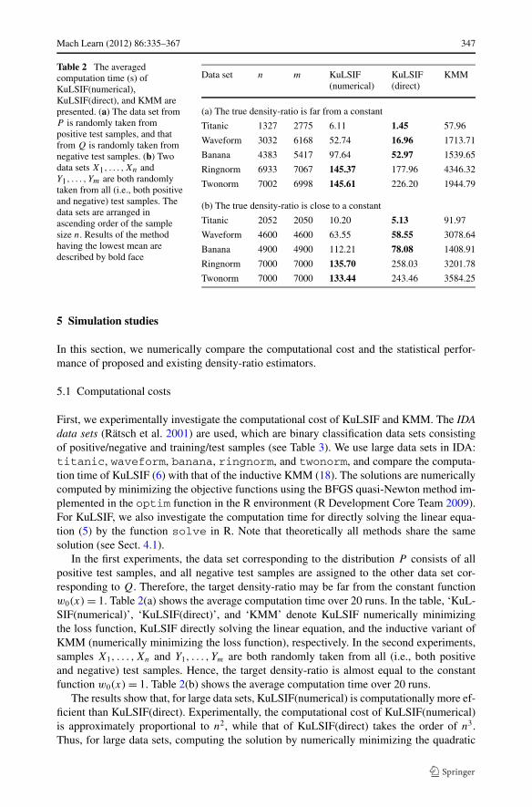
Table 2 The averagedcomputation time (s) ofKuLSIF(numerical),KuLSIF(direct), and KMM arepresented. (a) The data set fromP is randomly taken frompositive test samples, and thatfrom Q is randomly taken fromnegative test samples. (b) Twodata sets X1, . . . ,Xn andY1, . . . , Ym are both randomlytaken from all (i.e., both positiveand negative) test samples. Thedata sets are arranged inascending order of the samplesize n. Results of the methodhaving the lowest mean aredescribed by bold face

Data set n m KuLSIF(numerical)

KuLSIF(direct)

KMM

(a) The true density-ratio is far from a constant

Titanic 1327 2775 6.11 1.45 57.96

Waveform 3032 6168 52.74 16.96 1713.71

Banana 4383 5417 97.64 52.97 1539.65

Ringnorm 6933 7067 145.37 177.96 4346.32

Twonorm 7002 6998 145.61 226.20 1944.79

(b) The true density-ratio is close to a constant

Titanic 2052 2050 10.20 5.13 91.97

Waveform 4600 4600 63.55 58.55 3078.64

Banana 4900 4900 112.21 78.08 1408.91

Ringnorm 7000 7000 135.70 258.03 3201.78

Twonorm 7000 7000 133.44 243.46 3584.25

5 Simulation studies

In this section, we numerically compare the computational cost and the statistical perfor-mance of proposed and existing density-ratio estimators.

5.1 Computational costs

First, we experimentally investigate the computational cost of KuLSIF and KMM. The IDAdata sets (Rätsch et al. 2001) are used, which are binary classification data sets consistingof positive/negative and training/test samples (see Table 3). We use large data sets in IDA:titanic, waveform, banana, ringnorm, and twonorm, and compare the computa-tion time of KuLSIF (6) with that of the inductive KMM (18). The solutions are numericallycomputed by minimizing the objective functions using the BFGS quasi-Newton method im-plemented in the optim function in the R environment (R Development Core Team 2009).For KuLSIF, we also investigate the computation time for directly solving the linear equa-tion (5) by the function solve in R. Note that theoretically all methods share the samesolution (see Sect. 4.1).

In the first experiments, the data set corresponding to the distribution P consists of allpositive test samples, and all negative test samples are assigned to the other data set cor-responding to Q. Therefore, the target density-ratio may be far from the constant functionw0(x) = 1. Table 2(a) shows the average computation time over 20 runs. In the table, ‘KuL-SIF(numerical)’, ‘KuLSIF(direct)’, and ‘KMM’ denote KuLSIF numerically minimizingthe loss function, KuLSIF directly solving the linear equation, and the inductive variant ofKMM (numerically minimizing the loss function), respectively. In the second experiments,samples X1, . . . ,Xn and Y1, . . . , Ym are both randomly taken from all (i.e., both positiveand negative) test samples. Hence, the target density-ratio is almost equal to the constantfunction w0(x) = 1. Table 2(b) shows the average computation time over 20 runs.

The results show that, for large data sets, KuLSIF(numerical) is computationally more ef-ficient than KuLSIF(direct). Experimentally, the computational cost of KuLSIF(numerical)is approximately proportional to n2, while that of KuLSIF(direct) takes the order of n3.Thus, for large data sets, computing the solution by numerically minimizing the quadratic

348 Mach Learn (2012) 86:335–367

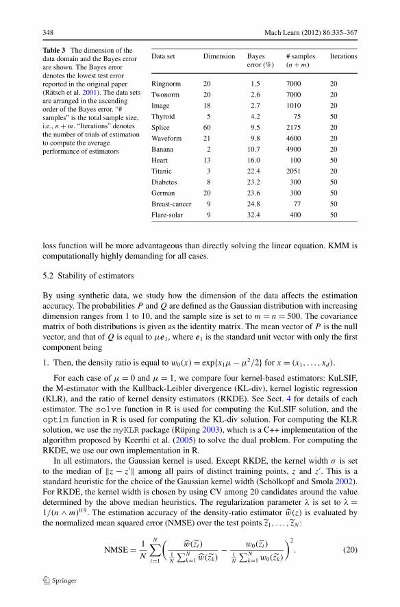
Table 3 The dimension of thedata domain and the Bayes errorare shown. The Bayes errordenotes the lowest test errorreported in the original paper(Rätsch et al. 2001). The data setsare arranged in the ascendingorder of the Bayes error. “#samples” is the total sample size,i.e., n + m. “Iterations” denotesthe number of trials of estimationto compute the averageperformance of estimators

Data set Dimension Bayeserror (%)

# samples(n + m)

Iterations

Ringnorm 20 1.5 7000 20

Twonorm 20 2.6 7000 20

Image 18 2.7 1010 20

Thyroid 5 4.2 75 50

Splice 60 9.5 2175 20

Waveform 21 9.8 4600 20

Banana 2 10.7 4900 20

Heart 13 16.0 100 50

Titanic 3 22.4 2051 20

Diabetes 8 23.2 300 50

German 20 23.6 300 50

Breast-cancer 9 24.8 77 50

Flare-solar 9 32.4 400 50

loss function will be more advantageous than directly solving the linear equation. KMM iscomputationally highly demanding for all cases.

5.2 Stability of estimators

By using synthetic data, we study how the dimension of the data affects the estimationaccuracy. The probabilities P and Q are defined as the Gaussian distribution with increasingdimension ranges from 1 to 10, and the sample size is set to m = n = 500. The covariancematrix of both distributions is given as the identity matrix. The mean vector of P is the nullvector, and that of Q is equal to μe1, where e1 is the standard unit vector with only the firstcomponent being

1. Then, the density ratio is equal to w0(x) = exp{x1μ − μ2/2} for x = (x1, . . . , xd).

For each case of μ = 0 and μ = 1, we compare four kernel-based estimators: KuLSIF,the M-estimator with the Kullback-Leibler divergence (KL-div), kernel logistic regression(KLR), and the ratio of kernel density estimators (RKDE). See Sect. 4 for details of eachestimator. The solve function in R is used for computing the KuLSIF solution, and theoptim function in R is used for computing the KL-div solution. For computing the KLRsolution, we use the myKLR package (Rüping 2003), which is a C++ implementation of thealgorithm proposed by Keerthi et al. (2005) to solve the dual problem. For computing theRKDE, we use our own implementation in R.

In all estimators, the Gaussian kernel is used. Except RKDE, the kernel width σ is setto the median of ‖z − z′‖ among all pairs of distinct training points, z and z′. This is astandard heuristic for the choice of the Gaussian kernel width (Schölkopf and Smola 2002).For RKDE, the kernel width is chosen by using CV among 20 candidates around the valuedetermined by the above median heuristics. The regularization parameter λ is set to λ =1/(n ∧ m)0.9. The estimation accuracy of the density-ratio estimator w(z) is evaluated bythe normalized mean squared error (NMSE) over the test points z1, . . . , zN :

NMSE = 1

N

N∑

i=1

(w(zi )

1N

∑N

k=1 w(zk)− w0(zi)

1N

∑N

k=1 w0(zk)

)2

. (20)

Mach Learn (2012) 86:335–367 349

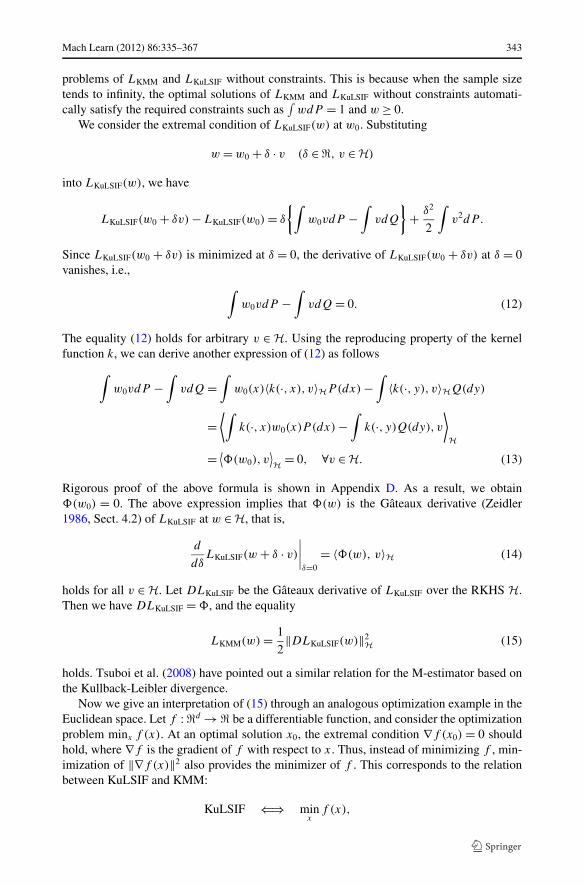
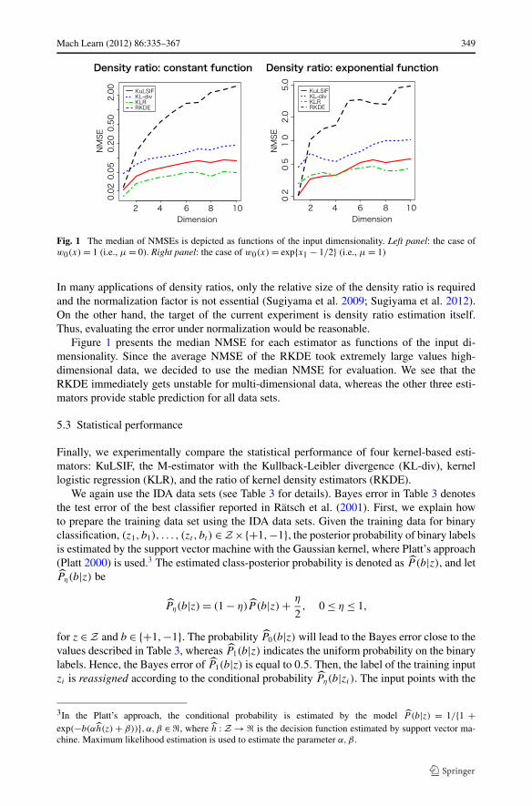
Fig. 1 The median of NMSEs is depicted as functions of the input dimensionality. Left panel: the case ofw0(x) = 1 (i.e., μ = 0). Right panel: the case of w0(x) = exp{x1 − 1/2} (i.e., μ = 1)

In many applications of density ratios, only the relative size of the density ratio is requiredand the normalization factor is not essential (Sugiyama et al. 2009; Sugiyama et al. 2012).On the other hand, the target of the current experiment is density ratio estimation itself.Thus, evaluating the error under normalization would be reasonable.

Figure 1 presents the median NMSE for each estimator as functions of the input di-mensionality. Since the average NMSE of the RKDE took extremely large values high-dimensional data, we decided to use the median NMSE for evaluation. We see that theRKDE immediately gets unstable for multi-dimensional data, whereas the other three esti-mators provide stable prediction for all data sets.

5.3 Statistical performance

Finally, we experimentally compare the statistical performance of four kernel-based esti-mators: KuLSIF, the M-estimator with the Kullback-Leibler divergence (KL-div), kernellogistic regression (KLR), and the ratio of kernel density estimators (RKDE).

We again use the IDA data sets (see Table 3 for details). Bayes error in Table 3 denotesthe test error of the best classifier reported in Rätsch et al. (2001). First, we explain howto prepare the training data set using the IDA data sets. Given the training data for binaryclassification, (z1, b1), . . . , (zt , bt ) ∈ Z ×{+1,−1}, the posterior probability of binary labelsis estimated by the support vector machine with the Gaussian kernel, where Platt’s approach(Platt 2000) is used.3 The estimated class-posterior probability is denoted as P (b|z), and letPη(b|z) be

Pη(b|z) = (1 − η)P (b|z) + η

2, 0 ≤ η ≤ 1,

for z ∈ Z and b ∈ {+1,−1}. The probability P0(b|z) will lead to the Bayes error close to thevalues described in Table 3, whereas P1(b|z) indicates the uniform probability on the binarylabels. Hence, the Bayes error of P1(b|z) is equal to 0.5. Then, the label of the training inputzi is reassigned according to the conditional probability Pη(b|zi). The input points with the

3In the Platt’s approach, the conditional probability is estimated by the model P (b|z) = 1/{1 +exp(−b(αh(z) + β))}, α,β ∈ , where h : Z → is the decision function estimated by support vector ma-chine. Maximum likelihood estimation is used to estimate the parameter α,β .

350 Mach Learn (2012) 86:335–367

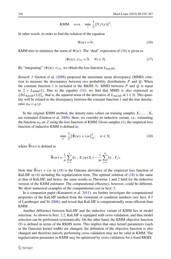
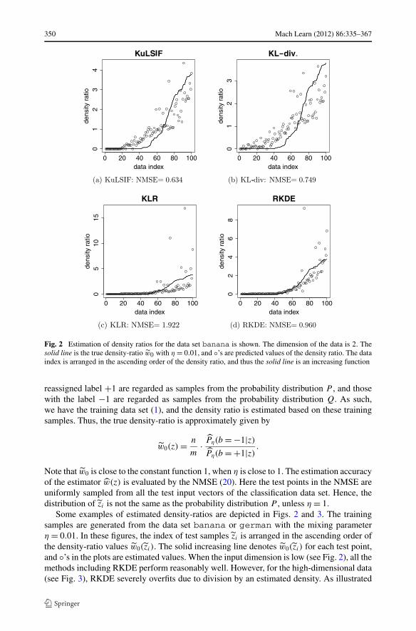
Fig. 2 Estimation of density ratios for the data set banana is shown. The dimension of the data is 2. Thesolid line is the true density-ratio w0 with η = 0.01, and ◦’s are predicted values of the density ratio. The dataindex is arranged in the ascending order of the density ratio, and thus the solid line is an increasing function

reassigned label +1 are regarded as samples from the probability distribution P , and thosewith the label −1 are regarded as samples from the probability distribution Q. As such,we have the training data set (1), and the density ratio is estimated based on these trainingsamples. Thus, the true density-ratio is approximately given by

w0(z) = n

m· Pη(b = −1|z)Pη(b = +1|z) .

Note that w0 is close to the constant function 1, when η is close to 1. The estimation accuracyof the estimator w(z) is evaluated by the NMSE (20). Here the test points in the NMSE areuniformly sampled from all the test input vectors of the classification data set. Hence, thedistribution of zi is not the same as the probability distribution P , unless η = 1.

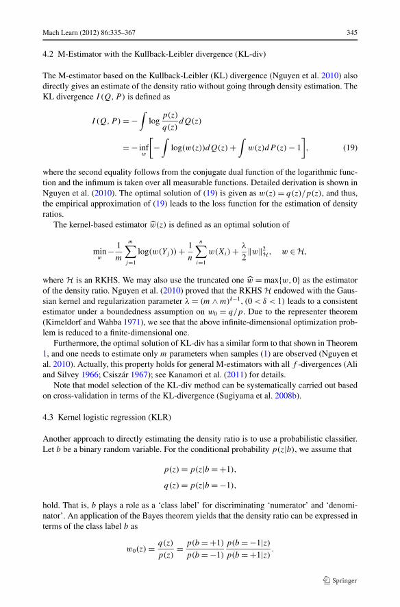
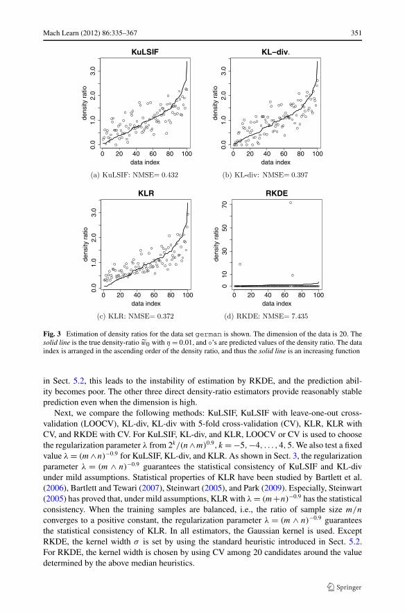
Some examples of estimated density-ratios are depicted in Figs. 2 and 3. The trainingsamples are generated from the data set banana or german with the mixing parameterη = 0.01. In these figures, the index of test samples zi is arranged in the ascending order ofthe density-ratio values w0(zi). The solid increasing line denotes w0(zi) for each test point,and ◦’s in the plots are estimated values. When the input dimension is low (see Fig. 2), all themethods including RKDE perform reasonably well. However, for the high-dimensional data(see Fig. 3), RKDE severely overfits due to division by an estimated density. As illustrated

Mach Learn (2012) 86:335–367 351

Fig. 3 Estimation of density ratios for the data set german is shown. The dimension of the data is 20. Thesolid line is the true density-ratio w0 with η = 0.01, and ◦’s are predicted values of the density ratio. The dataindex is arranged in the ascending order of the density ratio, and thus the solid line is an increasing function

in Sect. 5.2, this leads to the instability of estimation by RKDE, and the prediction abil-ity becomes poor. The other three direct density-ratio estimators provide reasonably stableprediction even when the dimension is high.

Next, we compare the following methods: KuLSIF, KuLSIF with leave-one-out cross-validation (LOOCV), KL-div, KL-div with 5-fold cross-validation (CV), KLR, KLR withCV, and RKDE with CV. For KuLSIF, KL-div, and KLR, LOOCV or CV is used to choosethe regularization parameter λ from 2k/(n∧m)0.9, k = −5,−4, . . . ,4,5. We also test a fixedvalue λ = (m∧n)−0.9 for KuLSIF, KL-div, and KLR. As shown in Sect. 3, the regularizationparameter λ = (m ∧ n)−0.9 guarantees the statistical consistency of KuLSIF and KL-divunder mild assumptions. Statistical properties of KLR have been studied by Bartlett et al.(2006), Bartlett and Tewari (2007), Steinwart (2005), and Park (2009). Especially, Steinwart(2005) has proved that, under mild assumptions, KLR with λ = (m+n)−0.9 has the statisticalconsistency. When the training samples are balanced, i.e., the ratio of sample size m/n

converges to a positive constant, the regularization parameter λ = (m ∧ n)−0.9 guaranteesthe statistical consistency of KLR. In all estimators, the Gaussian kernel is used. ExceptRKDE, the kernel width σ is set by using the standard heuristic introduced in Sect. 5.2.For RKDE, the kernel width is chosen by using CV among 20 candidates around the valuedetermined by the above median heuristics.

352 Mach Learn (2012) 86:335–367

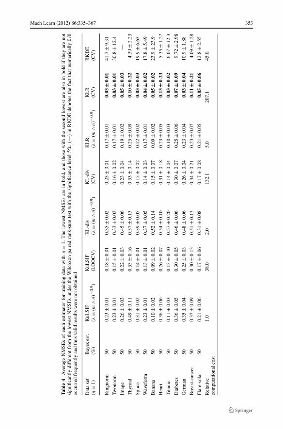
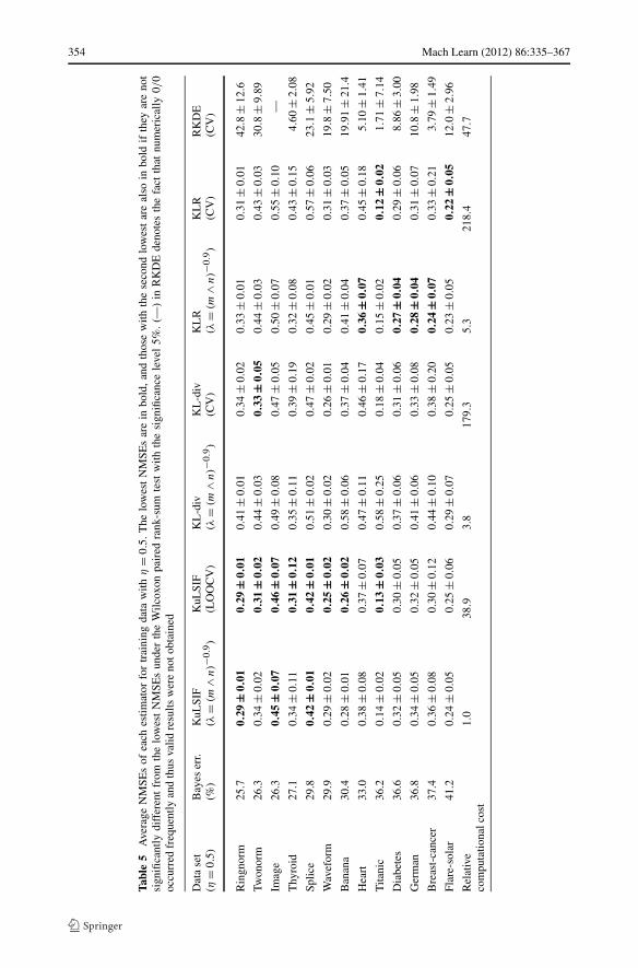
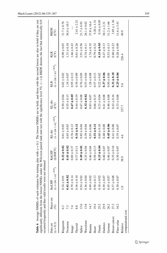
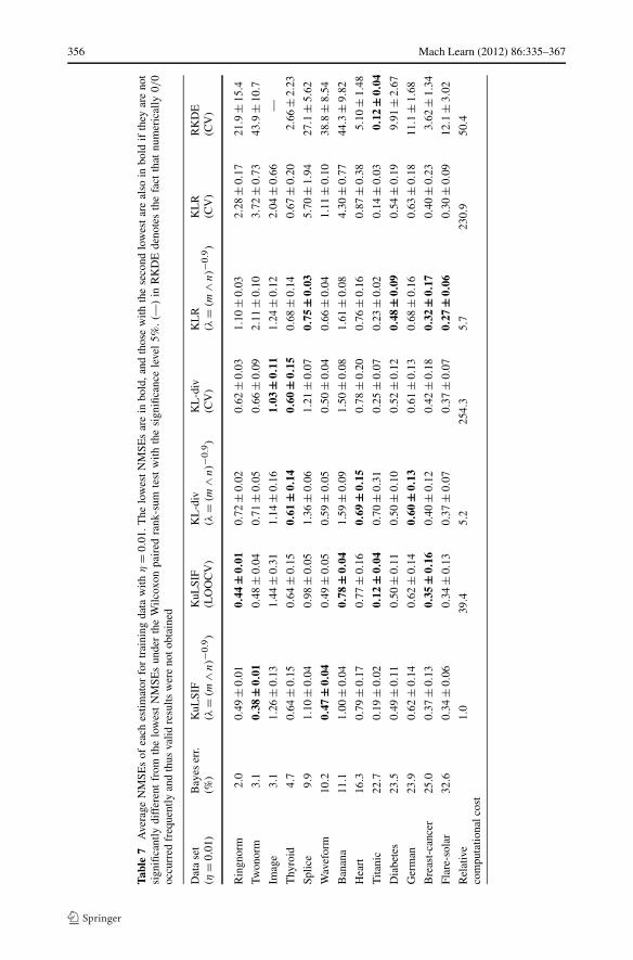
For each data set, training samples generated by setting η = 0.01,0.1,0.5 or 1 in Pη(b|z)are respectively prepared. For each training set, the NMSE of each estimator is computed. Byusing the NMSE over the uniformly distributed test samples, the estimation accuracy on thewhole data domain is evaluated, while Theorem 2 does not guarantee the statistical consis-tency for that test distribution. To compute the average performance, the above experimentsare repeated multiple times as described in Table 3. The numerical results are presented inTables 4–7 and Fig. 4. In the tables, data sets are arranged in the ascending order of theBayes error shown in Table 3. In Table 4, the NMSEs under η = 1 are presented. In thiscase, the class-posterior probability satisfies P1(b|z) = 0.5, and hence, the density ratio isclose to the constant function. Then, estimators with strong regularization will provide goodresults. Indeed, methods using LOOCV or CV such as KuLSIF(LOOCV), KL-div(CV), andKLR(CV) achieve the lowest NMSEs. Especially, KLR(CV) is significantly better than theothers. For small η, other estimators except RKDE also present good statistical performance(see Tables 5–7).

At the bottom of each table, the relative computational costs are also described. Thecomputation time depends on parameters included in the optimization algorithm. In order toreduce the computation time of KL-div and KL-div(CV), we used the optim function withthe stopping criterion reltol= 0.5 × 10−3, instead of the default value reltol= 10−8.On the other hand, KuLSIF using the solve function is numerically accurate. From theexperimental results, we see that KuLSIF dominates the other methods in terms of the com-putational efficiency. KuLSIF(LOOCV) with the analytic-form expression of the LOOCVscore also has a computational advantage over KL-div(CV), KLR(CV), and RKDE(CV).Note that the relative computational cost of KL-div is large for small η. This phenomenonis theoretically studied in a companion paper (Kanamori et al. 2011).

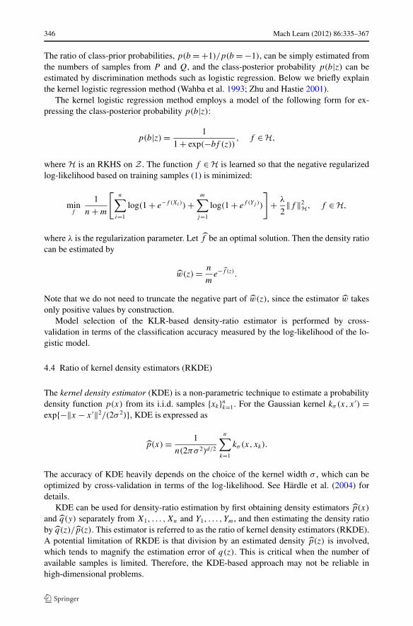
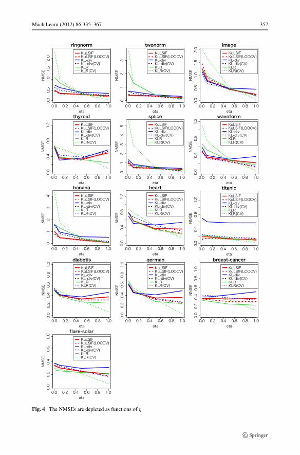
In Fig. 4, the NMSEs of estimators described in these tables are plotted as functions ofη. The NMSEs of RKDE are not shown since they are much larger than the others. We seethat KLR and KLR(CV) are sensitive to η for the data set with low Bayes error such asringnorm, twonorm, image, thyroid, splice, waveform, and banana. On theother hand, KuLSIF, KuLSIF(LOOCV), and KL-div(CV) present moderate NMSEs for awide range of η. See Tables 4–7 for more details.

6 Conclusions

In this paper, we addressed the problem of estimating the ratio of two probability densi-ties. We proposed a kernel-based least-squares density-ratio estimator called KuLSIF, andinvestigated its statistical properties such as consistency and the rate of convergence. Wealso showed that, not only the estimator, but also the leave-one-out cross-validation scorecan be analytically obtained for KuLSIF. This highly contributes to reducing the compu-tational cost. Then we pointed out that KuLSIF and an inductive variant of kernel meanmatching (KMM) actually share the same solution. Hence, the statistical properties of KuL-SIF are inherited to KMM. However, we showed through numerical experiments that KuL-SIF is computationally much more efficient than KMM. We further experimentally showedthat KuLSIF overall compares favorably with other density-ratio estimators such as the M-estimator with the Kullback-Leibler divergence, kernel logistic regression, and the ratio ofkernel density estimators.

Our definition of KuLSIF (see (4)) does not contain a non-negativity constraint on thelearned density-ratio function. We may add a non-negativity constraint w ≥ 0 to (4) asKanamori et al. (2009) did. However, by the additional constraint, we can no longer ob-tain the solution analytically. When the sample size is large, the estimator w obtained by (4)

Mach Learn (2012) 86:335–367 353

Tabl

e4

Ave

rage

NM

SEs

ofea

ches

timat

orfo

rtr

aini

ngda

taw

ithη

=1.

The

low

est

NM

SEs

are

inbo

ld,

and

thos

ew

ithth

ese

cond

low

est

are

also

inbo

ldif

they

are

not

sign

ifica

ntly

diff

eren

tfr

omth

elo

wes

tN

MSE

sun

der

the

Wilc

oxon

pair

edra

nk-s

umte

stw

ithth

esi

gnifi

canc

ele

vel

5%.

(—)

inR

KD

Ede

note

sth

efa

ctth

atnu

mer

ical

ly0/

0oc

curr

edfr

eque

ntly

and

thus

valid

resu

ltsw

ere

noto

btai

ned

Dat

ase

t(η

=1)

Bay

eser

r.(%

)K

uLSI

F(λ

=(m

∧n)−

0.9)

KuL

SIF

(LO

OC

V)

KL

-div

(λ=

(m∧n

)−0.

9)

KL

-div

(CV

)K

LR

(λ=

(m∧n

)−0.

9)

KL

R(C

V)

RK

DE

(CV

)

Rin

gnor

m50

0.23

±0.

010.

18±

0.01

0.35

±0.

020.

25±

0.01

0.17

±0.

010.

03±

0.01

41.7

±9.

31

Twon

orm

500.

23±

0.01

0.15

±0.

010.

33±

0.03

0.16

±0.

020.

17±

0.01

0.03

±0.

0130

.8±

12.4

Imag

e50

0.26

±0.

030.

22±

0 .03

0.45

±0.

060.

23±

0.04

0.19

±0.

020.

05±

0.03

—

Thy

roid

500.

49±

0.11

0.53

±0.

160.

57±

0.13

0.53

±0.

140.

25±

0.09

0.10

±0.

224.

39±

2.23

Splic

e50

0.31

±0.

020.

14±

0.01

0.39

±0.

050.

15±

0.02

0.22

±0.

020.

03±

0.03

19.9

±6.

63

Wav

efor

m50

0.23

±0.

010.

13±

0.01

0.37

±0.

050.

14±

0.03

0.17

±0.

010.

04±

0.02

17.8

±5.

49

Ban

ana

500.

10±

0.02

0.09

±0.

020.

52±

0.14

0.15

±0.

070.

09±

0.02

0.05

±0.

0223

.9±

23.9

Hea

rt50

0.36

±0.

060.

26±

0.07

0.54

±0.

100.

31±

0.18

0.23

±0.

050.

13±

0.23

5.35

±1.

27

Tita

nic

500.

11±

0.03

0.13

±0.

100.

57±

0.20

0.14

±0.

040.

10±

0.03

0.03

±0.

026.

07±

12.3

Dia

bete

s50

0.36

±0.

050.

30±

0.05

0.46

±0.

060.

30±

0.07

0.25

±0.

060.

07±

0.09

9.72

±2.

98

Ger

man

500.

35±

0.04

0.25

±0.

030.

48±

0.06

0.26

±0.

040.

23±

0.04

0.03

±0.

0410

.9±

1.88

Bre

ast-

canc

er50

0.37

±0.

090.

30±

0.13

0.51

±0.

130.

34±

0.21

0.23

±0.

070.

11±

0.21

4.09

±1.

28

Flar

e-so

lar

500.

21±

0.06

0.17

±0.

060.

31±

0.08

0.17

±0.

080.

21±

0.05

0.05

±0.

0612

.8±

2.55

Rel

ativ

eco

mpu

tatio

nalc

ost

1.0

38.0

2.0

132.

15.

020

7.1

45.0

354 Mach Learn (2012) 86:335–367

Tabl

e5

Ave

rage

NM

SEs

ofea

ches

timat

orfo

rtr

aini

ngda

taw

ithη

=0.

5.T

helo

wes

tN

MSE

sar

ein

bold

,an

dth

ose

with

the

seco

ndlo

wes

tar

eal

soin

bold

ifth

eyar

eno

tsi

gnifi

cant

lydi

ffer

ent

from

the

low

est

NM

SEs

unde

rth

eW

ilcox

onpa

ired

rank

-sum

test

with

the

sign

ifica

nce

leve

l5%

.(—

)in

RK

DE

deno

tes

the

fact

that

num

eric

ally

0/0

occu

rred

freq

uent

lyan

dth

usva

lidre

sults

wer

eno

tobt

aine

d

Dat

ase

t(η

=0.

5)B

ayes

err.

(%)

KuL

SIF

(λ=

(m∧n

)−0.

9)

KuL

SIF

(LO

OC

V)

KL

-div

(λ=

(m∧n

)−0.

9)

KL

-div

(CV

)K

LR

(λ=

(m∧n

)−0.

9)

KL

R(C

V)

RK

DE

(CV

)

Rin

gnor

m25

.70.

29±

0.01

0.29

±0.

010.

41±

0.01

0.34

±0.

020.

33±

0.01

0.31

±0.

0142

.8±

12.6

Twon

orm

26.3

0.34

±0.

020.

31±

0.02

0.44

±0.

030.

33±

0.05

0.44

±0.

030.

43±

0.03

30.8

±9.

89

Imag

e26

.30.

45±

0.07

0.46

±0.

070.

49±

0.08

0.47

±0.

050.

50±

0.07

0.55

±0.

10—

Thy

roid

27.1

0.34

±0.

110.

31±

0.12

0.35

±0.

110.

39±

0.19

0.32

±0.

080.

43±

0.15

4.60

±2.

08

Splic

e29

.80.

42±

0.01

0.42

±0.

010.

51±

0.02

0.47

±0.

020.

45±

0.01

0.57

±0.

0623

.1±

5.92

Wav

efor

m29

.90.

29±

0.02

0.25

±0.

020.

30±

0.02

0.26

±0.

010.

29±

0.02

0.31

±0.

0319

.8±

7.50

Ban

ana

30.4

0.28

±0.

010.

26±

0.02

0.58

±0.

060.

37±

0.04

0.41

±0.

040.

37±

0.05

19.9

1±

21.4

Hea

rt33

.00.

38±

0.08

0.37

±0.

070.

47±

0.11

0.46

±0.

170.

36±

0.07

0.45

±0.

185.

10±

1.41

Tita

nic

36.2

0.14

±0.

020.

13±

0.03

0.58

±0.

250.

18±

0.04

0.15

±0.

020.

12±

0.02

1.71

±7.

14

Dia

bete

s36

.60.

32±

0.05

0.30

±0.

050.

37±

0.06

0.31

±0.

060.

27±

0.04

0.29

±0.

068.

86±

3.00

Ger

man

36.8

0.34

±0.

050.

32±

0.05

0.41

±0.

060.

33±

0.08

0.28

±0.

040.

31±

0.07

10.8

±1.

98

Bre

ast-

canc

er37

.40.

36±

0.08

0.30

±0.

120.

44±

0.10

0.38

±0.

200.

24±

0.07

0.33

±0.

213.

79±

1.49

Flar

e-so

lar

41.2

0.24

±0.

050.

25±

0.06

0.29

±0.

070.

25±

0.05

0.23

±0.

050.

22±

0.05

12.0

±2.

96

Rel

ativ

eco

mpu

tatio

nalc

ost

1.0

38.9

3.8

179.

35.

321

8.4

47.7

Mach Learn (2012) 86:335–367 355

Tabl

e6

Ave

rage

NM

SEs

ofea

ches

timat

orfo

rtr

aini

ngda

taw

ithη

=0.

1.T

helo

wes

tN

MSE

sar

ein

bold

,an

dth

ose

with

the

seco

ndlo

wes

tar

eal

soin

bold

ifth

eyar

eno

tsi

gnifi

cant

lydi

ffer

ent

from

the

low

est

NM

SEs

unde

rth

eW

ilcox

onpa

ired

rank

-sum

test

with

the

sign

ifica

nce

leve

l5%

.(—

)in

RK

DE

deno

tes

the

fact

that

num

eric

ally

0/0

occu

rred

freq

uent

lyan

dth

usva

lidre

sults

wer

eno

tobt

aine

d

Dat

ase

t(η

=0.

1)B

ayes

err.

(%)

KuL

SIF

(λ=

(m∧n

)−0.

9)

KuL

SIF

(LO

OC

V)

KL

-div

(λ=

(m∧n

)−0.

9)

KL

-div

(CV

)K

LR

(λ=

(m∧n

)−0.

9)

KL

R(C

V)

RK

DE

(CV

)

Rin

gnor

m6.

30.

34±

0.01

0.32

±0.

020.

61±

0.02

0.50

±0.

040.

82±

0.02

0.98

±0.

0331

.7±

8.78

Twon

orm

7.3

0.41

±0.

020.

41±

0.02

0.65

±0.

030.

55±

0.13

1.34

±0.

071.

31±

0.10

36.4

±10

.3

Imag

e7.

40.

79±

0.14

0.89

±0 .

370.

76±

0.12

0.67

±0.

050.

95±

0.12

1.66

±0.

43—

Thy

roid

8.8

0.36

±0.

100.

37±

0.11

0.31

±0.

110.

44±

0.19

0.39

±0.

090.

61±

0.26

2.41

±2.

21

Splic

e13

.60.

54±

0.02

0.49

±0.

010.

85±

0.04

0.67

±0.

080.

76±

0.05

2.91

±0.

5621

.7±

6.93

Wav

efor

m13

.80.

36±

0.04

0.35

±0.

040.

39±

0.04

0.32

±0.

020.

53±

0.04

0.74

±0.

1126

.1±

9.02

Ban

ana

14.7

0.49

±0.

020.

46±

0.04

0.93

±0.

060.

83±

0.07

1.28

±0.

081.

74±

0.35

37.8

±16

.4

Hea

rt19

.40.

58±

0.13

0.58

±0.

130.

51±

0.11

0.66

±0.

150.

57±

0.13

0.79

±0.

325.

20±

1.31

Tita

nic

25.2

0.18

±0.

020.

15±

0.04

0.60

±0.

180.

23±

0.04

0.22

±0.

020.

15±

0.03

0.16

±0.

05

Dia

bete

s25

.90.

39±

0.07

0.40

±0.

070.

40±

0.08

0.41

±0.

080.

37±

0.06

0.47

±0.

1310

.1±

2.31

Ger

man

26.2

0.45

±0.

070.

46±

0.07

0.45

±0.

060.

46±

0.08

0.50

±0.

080.

53±

0.13

11.2

±1.

66

Bre

ast-

canc

er27

.30.

37±

0.08

0.35

±0.

100.

41±

0.08

0.43

±0.

160.

31±

0.10

0.40

±0.

233.

85±

1.36

Flar

e-so

lar

34.2

0.30

±0.

070.

30±

0.07

0.35

±0.

070.

33±

0.08

0.25

±0.

060.

28±

0.09

11.6

±3.

43

Rel

ativ

eco

mpu

tatio

nalc

ost

1.0

38.9

4.6

237.

75.

622

6.4

49.9

356 Mach Learn (2012) 86:335–367

Tabl

e7

Ave

rage

NM

SEs

ofea

ches

timat

orfo

rtr

aini

ngda

taw

ithη

=0.

01.T

helo

wes

tN

MSE

sar

ein

bold

,and

thos

ew

ithth

ese

cond

low

est

are

also

inbo

ldif

they

are

not

sign

ifica

ntly

diff

eren

tfr

omth

elo

wes

tN

MSE

sun

der

the

Wilc

oxon

pair

edra

nk-s

umte

stw

ithth

esi

gnifi

canc

ele

vel

5%.

(—)

inR

KD

Ede

note

sth

efa

ctth

atnu

mer

ical

ly0/

0oc

curr

edfr

eque

ntly

and

thus

valid

resu

ltsw

ere

noto

btai

ned

Dat

ase

t(η

=0.

01)

Bay

eser

r.(%

)K

uLSI

F(λ

=(m

∧n)−

0.9)

KuL

SIF

(LO

OC

V)

KL

-div

(λ=

(m∧n

)−0.

9)

KL

-div

(CV

)K

LR

(λ=

(m∧n

)−0.

9)

KL

R(C

V)

RK

DE

(CV

)

Rin

gnor

m2.

00.

49±

0.01

0.44

±0.

010.

72±

0.02

0.62

±0.

031.

10±

0.03

2.28

±0.

1721

.9±

15.4

Twon

orm

3.1

0.38

±0.

010.

48±

0.04

0.71

±0.

050.

66±

0.09

2.11

±0.

103.

72±

0.73

43.9

±10

.7

Imag

e3.

11.

26±

0 .13

1.44

±0.

311.

14±

0.16

1.03

±0.

111.

24±

0.12

2.04

±0.

66—

Thy

roid

4.7

0.64

±0.

150.

64±

0.15

0.61

±0.

140.

60±

0.15

0.68

±0.

140.

67±

0.20

2.66

±2.

23

Splic

e9.

91.

10±

0.04

0.98

±0.

051.

36±

0.06

1.21

±0.

070.

75±

0.03

5.70

±1.

9427

.1±

5.62

Wav

efor

m10

.20.

47±

0.04

0.49

±0.

050.

59±

0.05

0.50

±0.

040.

66±

0.04

1.11

±0.

1038

.8±

8.54

Ban

ana

11.1

1.00

±0.

040.

78±

0.04

1.59

±0.

091.

50±

0.08

1.61

±0.

084.

30±

0.77

44.3

±9.

82

Hea

rt16

.30.

79±

0.17

0.77

±0.

160.

69±

0.15

0.78

±0.

200.

76±

0.16

0.87

±0.

385.

10±

1.48

Tita

nic

22.7

0.19

±0.

020.

12±

0.04

0.70

±0.

310.

25±

0.07

0.23

±0.

020.

14±

0.03

0.12

±0.

04

Dia

bete

s23

.50.

49±

0.11

0.50

±0.

110.

50±

0.10

0.52

±0.

120.

48±

0.09

0.54

±0.

199.

91±

2.67

Ger

man

23.9

0.62

±0.

140.

62±

0.14

0.60

±0.

130.

61±

0.13

0.68

±0.

160.

63±

0.18

11.1

±1.

68

Bre

ast-

canc

er25

.00.

37±

0.13

0.35

±0.

160.

40±

0.12

0.42

±0.

180.

32±

0.17

0.40

±0.

233.

62±

1.34

Flar

e-so

lar

32.6

0.34

±0.

060.

34±

0.13

0.37

±0.

070.

37±

0.07

0.27

±0.

060.

30±

0.09

12.1

±3.

02

Rel

ativ

eco

mpu

tatio

nalc

ost

1.0

39.4

5.2

254.

35.

723

0.9

50.4

Mach Learn (2012) 86:335–367 357

Fig. 4 The NMSEs are depicted as functions of η

358 Mach Learn (2012) 86:335–367

will be a non-negative function without additional constraints. Thus, the estimator w (andits cut-off version w+) will be asymptotically the same as the one obtained by imposingthe nonnegative constraint on (4). For the small sample size, however, the estimator w cantake negative values, and the cut-off estimator w+ may have statistical bias. Thus, we needcareful treatment to obtain a good estimator in practice. In nonparametric density estima-tion, it was shown that nonnegative estimators cannot be unbiased (Rosenblatt 1956). Weconjecture that a similar result also holds in the inference of density ratios, which needs tobe investigated in our future work.

Acknowledgements The authors are grateful to the anonymous reviewers for their helpful comments. Thework of T. Kanamori was partially supported by Grant-in-Aid for Young Scientists (20700251). T. Suzukiwas supported in part by Global COE Program “The research and training center for new development inmathematics”, MEXT, Japan. M. Sugiyama was supported by SCAT, AOARD, and the JST PRESTO pro-gram.

Appendix A: Proof of Theorem 1

Proof Applying the representer theorem (Kimeldorf and Wahba 1971), we see that an opti-mal solution of (4) has the form of

w =n∑

j=1

αjk(·,Xj ) +m∑

�=1

β�k(·, Y�). (21)

Let K11, K12, K21, and K22 be the sub-matrices of the Gram matrix:

(K11)ii′ = k(Xi,Xi′), (K12)ij = k(Xi, Yj ), K21 = K�12, (K22)jj ′ = k(Yj , Yj ′),

where i, i ′ = 1, . . . , n, j, j ′ = 1, . . . ,m. Then, the extremal condition of (4) with respect toparameters α = (α1, . . . , αn)

� and β = (β1, . . . , βn)� is given as

1

nK11(K11α + K12β) − 1

mK121m + λK11α + λK12β = 0, and

1

nK21(K11α + K12β) − 1

mK221m + λK22β + λK21α = 0.

An easy computation shows that the above extremal condition is satisfied at the parameterα which is defined as the solution of the linear (5) and β = 1

mλ(1, . . . ,1)�. �

Appendix B: Leave-one-out cross-validation of KuLSIF

The procedure to compute the leave-one-out cross-validation score of KuLSIF is presentedhere. Let K

(�)

11 ∈ (n−1)×(n−1) and K(�)

12 = K(�)�21 ∈ (n−1)×(m−1) be the Gram matrices of sam-

ples except x� and y�, respectively. According to Theorem 1, the estimated parameters α(�)

and β(�) of

w(�)(z) =∑

i �=�

αik(z,Xi) +∑

j �=�

βj k(z,Yj )

Mach Learn (2012) 86:335–367 359

is equal to

α(�) = − 1

(m − 1)λ(K

(�)

11 + (n − 1)λIn−1)−1K

(�)

12 1m−1, β(�) = 1

(m − 1)λ1m−1,

where In−1 denotes the (n − 1) by (n − 1) identity matrix. Hence, the parameter α(�) is thesolution of the following convex quadratic problem,

minα

1

2α�(K

(�)

11 + (n − 1)λIn−1)α + 1

(m − 1)λ1�

m−1K(�)

21 α, α ∈ n−1.

The same solution can be obtained by solving

minα

1

2α�(K11 + (n − 1)λIn)α + 1

(m − 1)λ(1m − em,�)

�K21α,

s.t. α ∈ n, α� = 0,

(22)

where em,� ∈ m is the standard unit vector with only the �-th component being 1. Theoptimal solution of (22) denoted by α(�) is equal to

α(�) = (K11 + (n − 1)λIn)−1

(

− 1

(m − 1)λK12(1m − em,�) − c�en,�

)

,

where c� is determined so that α(�)� = 0. The estimator α(�) ∈ n−1 is equal to the

(n − 1)-dimensional vector consisting of α(�) except the �-th component, i.e., α(�) =(α

(�)

1 , . . . , α(�)

�−1, α(�)

�+1, . . . , α(�)n )�. Let β(�) be

β(�) = 1

(m − 1)λ(1m − em,�),

then we have

w(�)(z) =n∑

i=1

α(�)i k(z,Xi) +

m∑

j=1

β(�)j k(z,Yj ).

We consider an analytic expression of the leave-one-out score. Let the matrices A and B

be the parameters of the leave-one-out estimator,

A = (α(1), . . . , α(n∧m)) ∈ n×(n∧m), B = (β(1), . . . , β(n∧m)) ∈ m×(n∧m),

the matrix G ∈ n×n be G = (K11 + (n− 1)λIn)−1, and E ∈ m×(n∧m) be the matrix defined

as

Eij ={

1 i �= j,

0 i = j.

Let S ∈ n×(n∧m) be

S = − 1

(m − 1)λK12E,

and T ∈ n×(n∧m) be

Tij =⎧⎨

⎩

(GS)ii

Gii

i = j,

0 i �= j.

360 Mach Learn (2012) 86:335–367

Then, we obtain

A = G(S − T ), B = 1

(m − 1)λE.

Let KX ∈ (n∧m)×(n+m) be the sub-matrix of (K11K12) formed by the first n ∧ m rows andall columns. Similarly, let KY ∈ (n∧m)×(n+m) be the sub-matrix of (K21K22) formed by thefirst n ∧ m rows and all columns. Let the product U ∗ U ′ be the element-wise multiplicationof matrices U and U ′ of the same size, i.e., the (i, j) element is given by UijU

′ij . Then, we

have

wX = (w(1)(X1), . . . , w(n∧m)(Xn∧m))� = (KX ∗ (A� B�))1n+m,

wY = (w(1)(Y1), . . . , w(n∧m)(Yn∧m))� = (KY ∗ (A� B�))1n+m,

wX+ = (w(1)+ (X1), . . . , w

(n∧m)+ (Xn∧m))� = max{wX,0},

wY+ = (w(1)+ (Y1), . . . , w

(n∧m)+ (Yn∧m))� = max{wY ,0},

where the max operation for a vector is applied in the element-wise manner. As a result,LOOCV (7) is equal to

LOOCV = 1

n ∧ m

{1

2w�

X+wX+ − 1�n∧mwY+

}

.

Appendix C: Proof of Theorem 2

We summarize some notations to be used in the proof. Given a probability distribution P

and a random variable h(X), we denote the expectation of h(X) under P by∫

hdP . Givensamples X1, . . . ,Xn from P , the empirical distribution is denoted by Pn. The expectation∫

hdPn denotes the empirical means of h(X), that is, 1n

∑n

i=1 h(Xi). We also use the notation∫hd(P − Pn) to represent

∫hdP − 1

n

∑n

i=1 h(Xi). Let H be the RKHS endowed with thekernel k. The norm and inner product on H are denoted by ‖ · ‖H and 〈·, ·〉H , respectively.Let ‖ · ‖∞ be the infinity norm, and for distribution function P , define the L2 norm by

‖g‖P =(∫

|g|2dP

)1/2

,

and let L2(P ) be the metric space defined by this distance.Since supx∈Z k(x, x) is assumed to be bounded above, without loss of generality we

assume supx∈Z k(x, x) ≤ 1. The constant factor of the kernel function does not affect thefollowing proof.

We now define the bracketing entropy of the set of functions. For any fixed δ > 0,a covering for function class F using the metric L2(P ) is a collection of functionswhich allows F to be covered using L2(P ) balls of radius δ centered at these functions.Let NB(δ, F ,P ) be the smallest number of N for which there exist pairs of functions{(gL

j , gUj ) ∈ L2(P ) × L2(P )|j = 1, . . . ,N} such that ‖gL

j − gUj ‖P ≤ δ, and such that for

each f ∈ F , there exists j satisfying gLj ≤ f ≤ gU

j . Then, HB(δ, F ,P ) = logNB(δ, F ,P )

is called the bracketing entropy of F (van de Geer 2000, Definition 2.2).

Mach Learn (2012) 86:335–367 361

For w ∈ H, we have ‖w‖P ≤ ‖w‖∞ ≤ ‖w‖H , because for any x ∈ Z , the inequalities

|w(x)| = |〈w,k(·, x)〉H| ≤ ‖w‖H supx

√k(x, x) ≤ ‖w‖H

hold. Let G = {v2|v ∈ H} and we define a measure of complexity J : G → by

J (g) = inf { ‖v‖2H|g = v2, v ∈ H }.

Let HM and G M be

HM ={v ∈ H|‖v‖H < M},(23)

GM ={v2|v ∈ H√M} = {g ∈ G|J (g) < M}.

It is straightforward to verify the second equality of (23).The following proposition is crucial to prove the convergence property of KuLSIF.

Proposition 1 (Lemma 5.14 in van de Geer 2000) Let F ⊂ L2(P ) be a function class, andthe map I (f ) be a measure of complexity of f ∈ F , where I is a non-negative functional onF and I (f0) < ∞ for a fixed f0 ∈ F . We now define FM = {f ∈ F |I (f ) < M} satisfyingF = ∪M≥1 FM . Suppose that there exist c0 > 0 and 0 < γ < 2 such that

supf ∈FM

‖f − f0‖P ≤ c0M, supf ∈FM‖f −f0‖P ≤δ

‖f − f0‖∞ ≤ c0M, for all δ > 0,

and that HB(δ, FM,P ) = O(M/δ)γ . Then, we have

supf ∈F

∣∣∫(f − f0)d(P − Pn)

∣∣

D(f )= Op(1) (n → ∞),

where D(f ) is defined by

D(f ) = ‖f − f0‖1−γ /2P I (f )γ/2

√n

∨ I (f )

n2/(2+γ )

and a ∨ b denotes max{a, b}.

In van de Geer (2000), the probabilistic order is evaluated for each case of ‖f − f0‖ ≤n−1/(2+γ )I (f ) and ‖f − f0‖ > n−1/(2+γ )I (f ), respectively. When the supremum is takenover {f ∈ F |‖f − f0‖ ≤ n−1/(2+γ )I (f )}, D(f ) is equal to I (f )/n2/(2+γ ), and the proba-bilistic order above is obtained from the first formula of Lemma 5.14 (van de Geer 2000).In the same way, we obtain the probabilistic order for ‖f − f0‖ > n−1/(2+γ )I (f ). The sumof the probabilistic upper bounds for these two cases provides the result in the above propo-sition.

We use Proposition 1 to derive an upper bound of

∫(w − w0)d(Q − Qm) and

∫(w2 − w2

0)d(P − Pn).

362 Mach Learn (2012) 86:335–367

Lemma 1 The bracketing entropy of GM is bounded above by

HB(δ, G M,P ) = O

(M

δ

)γ

.

Proof Let vL1 , vU

1 , vL2 , vU

2 , . . . , vLN , vU

N ∈ L2(P ) be coverings of H√M in the sense of brack-

eting, such that ‖vLi − vU

i ‖P ≤ δ holds for i = 1, . . . ,N . Then, for any v ∈ H√M there exists

i such that vLi ≤ v ≤ vU

i holds. We can choose these functions such that ‖vL(U)i ‖∞ ≤ √

M issatisfied for all i = 1, . . . ,N , since for any v ∈ H√

M , the inequality ‖v‖∞ ≤ ‖v‖H <√

M

holds. For example, replace vL(U)i with min{√M ,max{−√

M,vL(U)i }} ∈ L2(P ). Let vL

i andvU

i be

vLi (x) =

⎧⎨

⎩

(vLi (x))2, vL

i (x) ≥ 0,

(vUi (x))2, vU

i (x) ≤ 0,

0, vLi (x) < 0 < vU

i (x),

vUi = max{(vL

i )2, (vUi )2},

for i = 1, . . . ,N . Then, vLi ≤ vU

i holds. Moreover, for any v ∈ H√M satisfying vL

i ≤ v ≤ vUi ,

we have vLi ≤ v2 ≤ vU

i . By definition, we also have

0 ≤vUi (x) − vL

i (x) ≤ max{|vUi (x)2 − vL

i (x)2|, |vUi (x) − vL

i (x)|2}≤(|vU

i (x)| + |vLi (x)|) · |vU

i (x) − vLi (x)| ≤ 2

√M|vU

i (x) − vLi (x)|,

and thus, ‖vUi − vL

i ‖P ≤ 2√

M‖vUi − vL

i ‖P holds. Due to (8), we obtain

HB(2√

Mδ, G M,P ) ≤ HB(δ, H√M,P ) = O

(√M

δ

)γ

.

Hence, HB(δ, G M,P ) = O(M/δ)γ holds. �

Lemma 2 Assume the condition of Theorem 2. Then, for the KuLSIF estimator w, we have

∣∣∣∣

∫(w − w0)d(Q − Qm)

∣∣∣∣ =Op

(‖w0 − w‖1−γ /2P ‖w‖γ /2

H√m

∨ ‖w‖H

m2/(2+γ )

)

,

∣∣∣∣

∫(w2 − w2

0)d(P − Pn)

∣∣∣∣ =Op

(‖w − w0‖1−γ /2P (1 + ‖w‖H)1+γ /2

√n

∨ ‖w‖2H

n2/(2+γ )

)

.

Proof There exists c0 > 0 such that

supw∈HM

‖w − w0‖P ≤ c0M, supw∈HM‖w−w0‖P ≤δ

‖w − w0‖∞ ≤ c0M, (24)

supg∈GM

‖g − w20‖P ≤ c0M, sup

g∈GM

‖g−w20‖P ≤δ

‖g − w20‖∞ ≤ c0M. (25)

The inequalities in (25) are derived as follows. For g ∈ GM , there exists v ∈ H such thatv2 = g and ‖v‖2

H < M , and then, we have

‖g − w20‖P ≤ ‖g − w2

0‖∞ ≤ ‖v‖2∞ + ‖w0‖2

∞

Mach Learn (2012) 86:335–367 363

≤ ‖v‖2H + ‖w0‖2

∞ ≤ M + ‖w0‖2∞ ≤ c0M (M ≥ 1).

In the same way, (24) also holds.Set F be H and I (w) = ‖w‖H in Proposition 1. Taking (24) into account, we have

supw∈H

∣∣∫(w0 − w)d(Q − Qm)

∣∣

D(w)= Op(1),

where D(w) is defined as

D(w) = ‖w0 − w‖1−γ /2P ‖w‖γ /2

H√m

∨ ‖w‖H

m2/(2+γ ).

In the same way, by setting F be G and I (g) = J (g) in Proposition 1, we have

supw∈H

∣∣∫(w2 − w2

0)d(P − Pn)∣∣

E(w)= Op(1),

where E(w) is defined as

E(w) = ‖w2 − w20‖1−γ /2

P J (w2)γ/2

√n

∨ J (w2)

n2/(2+γ ).

Note that ‖w2 − w20‖P ≤ (‖w0‖∞ + ‖w‖H)‖w − w0‖P = O((1 + ‖w‖H)‖w − w0‖P ) and

J (w2) ≤ ‖w‖2H . Then, we obtain

E(w) ≤‖w − w0‖1−γ /2P (1 + ‖w‖H)1+γ /2

√n

∨ ‖w‖2H

n2/(2+γ ).

�

Now we show the proof of Theorem 2.

Proof The estimator w satisfies the inequality

1

2

∫w2dPn −

∫wdQm + λ

2‖w‖2

H ≤ 1

2

∫w2

0dPn −∫

w0dQm + λ

2‖w0‖2

H.

Then, we have

1

2‖w − w0‖2

P =∫

(w0 − w)dQ + 1

2

∫(w2 − w2

0)dP

≤∫

(w0 − w)dQ + 1

2

∫(w2 − w2

0)dP

+∫

(w − w0)dQm + 1

2

∫(w2

0 − w2)dPn + λ

2‖w0‖2

H − λ

2‖w‖2

H.

As a result, we have

1

2‖w − w0‖2

P + λ

2‖w‖2

H

364 Mach Learn (2012) 86:335–367

≤∣∣∣∣

∫(w − w0)d(Q − Qm)

∣∣∣∣ + 1

2

∣∣∣∣

∫(w2 − w2

0)d(P − Pn)

∣∣∣∣ + λ

2‖w0‖2

H

≤ λ

2‖w0‖2

H + Op

(‖w0 − w‖1−γ /2P (1 + ‖w‖H)1+γ /2

√n ∧ m

∨ (1 + ‖w‖H)2

(n ∧ m)2/(2+γ )

)

,

where Lemma 2 is used.We need to study three possibilities:

1

2‖w0 − w‖2

P + λ

2‖w‖2

H ≤ Op(λ), (26)

1

2‖w0 − w‖2

P + λ

2‖w‖2

H ≤ Op

(‖w0 − w‖1−γ /2P (1 + ‖w‖H)1+γ /2

√n ∧ m

)

, (27)

1

2‖w0 − w‖2

P + λ

2‖w‖2

H ≤ Op

((1 + ‖w‖H)2

(n ∧ m)2/(2+γ )

)

. (28)

One of the above inequalities should be satisfied. We study each inequality below.Case (26): we have

1

2‖w0 − w‖2

P ≤ Op(λ),λ

2‖w‖2

H ≤ Op(λ),

and hence the inequalities ‖w0 − w‖P ≤ Op(λ1/2) and ‖w‖H ≤ Op(1) hold.Case (27): we have

‖w0 − w‖2P ≤ Op

(‖w0 − w‖1−γ /2P (1 + ‖w‖H)1+γ /2

(n ∧ m)1/2

)

,

λ‖w‖2H ≤ Op

(‖w0 − w‖1−γ /2P (1 + ‖w‖H)1+γ /2

(n ∧ m)1/2

)

.

The first inequality provides

‖w0 − w‖P ≤ Op

(1 + ‖w‖H

(n ∧ m)1/(2+γ )

)

.

Thus, the second inequality leads to

λ‖w‖2H ≤Op

(‖w0 − w‖1−γ /2P (1 + ‖w‖H)1+γ /2

(n ∧ m)1/2

)

≤Op

((1 + ‖w‖H

(n ∧ m)1/(2+γ )

)1−γ /2(1 + ‖w‖H)1+γ /2

(n ∧ m)1/2

)

=Op

((1 + ‖w‖H)2

(n ∧ m)2/(2+γ )

)

.

Hence, we have

‖w‖H ≤ Op

(1

λ1/2(n ∧ m)1/(2+γ )

)

= op(1).

Mach Learn (2012) 86:335–367 365

Then, we obtain

‖w0 − w‖P ≤ Op

(1

(n ∧ m)1/(2+γ )

)

≤ Op(λ1/2).

Case (28): we have

‖w0 − w‖2P ≤ Op

((1 + ‖w‖H)2

(n ∧ m)2/(2+γ )

)

, λ‖w‖2H ≤ Op

((1 + ‖w‖H)2

(n ∧ m)2/(2+γ )

)

.

Then, as shown in the case (27), we have ‖w‖H = op(1). Hence, we obtain

‖w0 − w‖P ≤ Op

(1

(n ∧ m)1/(2+γ )

)

≤ Op(λ1/2).

�

Appendix D: Proof of (13)

Theorem 3 Let H be the reproducing kernel Hilbert space endowed with the kernel functionk on Z × Z , and suppose supx∈Z k(x, x) < ∞. Then, for w,v ∈ H, the equality

∫wvdP −

∫vdQ = 〈�(w), v〉H

holds, where �(w) is defined by (11).

Proof For all w ∈ H, supx∈Z |w(x)| is bounded. This is because |w(x)| = |〈w,k(·, x)〉H| ≤‖w‖H

√k(x, x) < ∞. For a fixed w ∈ H, the function

∫wvdP − ∫

vdQ is linear andbounded as the function of v ∈ H. Indeed, the linearity is clear, and the boundedness isshown by

∣∣∣∣

∫wvdP −

∫vdQ

∣∣∣∣ ≤

∫|v(x)||w(x)|P (dx) +

∫|v(y)|Q(dy)

=∫

|〈v, k(·, x)〉H||w(x)|P (dx) +∫

|〈v, k(·, y)〉H|Q(dy)

≤ supx∈Z

√k(x, x)

(∫|w(x)|P (dx) + 1

)

‖v‖H.

Since |w(x)| is bounded, the integral above is finite. Then, by the Riesz representation the-orem (Reed and Simon 1972, Theorem II.4), there exists � : H → H such that

∫wvdP −

∫vdQ = 〈�(w), v〉H

holds for all w,v ∈ H. For v = k(·, x0) ∈ H, we have

(�(w))(x0) =∫

k(x0, x)w(x)P (dx) −∫

k(x0, y)Q(dy),

where we used the symmetry of the kernel function. We see that the function � is the sameas the function � defined by (11). �

366 Mach Learn (2012) 86:335–367

References

Ali, S. M., & Silvey, S. D. (1966). A general class of coefficients of divergence of one distribution fromanother. Journal of the Royal Statistical Society, Series B, 28, 131–142.

Aronszajn, N. (1950). Theory of reproducing kernels. Transactions of the American Mathematical Society,68, 337–404.

Bartlett, P. L., & Tewari, A. (2007). Sparseness vs estimating conditional probabilities: some asymptoticresults. Journal of Machine Learning Research, 8, 775–790.

Bartlett, P. L., Jordan, M. I., & McAuliffe, J. D. (2006). Convexity, classification, and risk bounds. Journal ofthe American Statistical Association, 101, 138–156.

Bickel, S., Brückner, M., & Scheffer, T. (2007). Discriminative learning for differing training and test distri-butions. In Proceedings of the 24th international conference on machine learning (pp. 81–88).

Bickel, S., Brückner, M., & Scheffer, T. (2009). Discriminative learning under covariate shift. Journal ofMachine Learning Research, 10, 2137–2155.

Csiszár, I. (1967). Information-type measures of difference of probability distributions and indirect observa-tion. Studia Scientiarum Mathematicarum Hungarica, 2, 229–318.

Cucker, F., & Smale, S. (2002). On the mathematical foundations of learning. Bulletin of the American Math-ematical Society, 39, 1–49.

Golub, G. H., & Loan, C. F. V. (1996). Matrix computations. Baltimore: Johns Hopkins University Press.Gretton, A., Borgwardt, K. M., Rasch, M. J., Schölkopf, B., & Smola, A. J. (2006). A kernel method for the

two-sample-problem. Advances in Neural Information Processing Systems, 19, 513–520.Gretton, A., Smola, A., Huang, J., Schmittfull, M., Borgwardt, K., & Schölkopf, B. (2009). Covariate shift

by kernel mean matching. In J. Quiñonero-Candela, M. Sugiyama, A. Schwaighofer, & N. Lawrence(Eds.), Dataset shift in machine learning, Chap. 8 (pp. 131–160). Cambridge: MIT Press.

Härdle, W., Müller, M., Sperlich, S., & Werwatz, A. (2004). Nonparametric and semiparametric models.Springer series in statistics. Berlin: Springer.

Hido, S., Tsuboi, Y., Kashima, H., Sugiyama, M., & Kanamori, T. (2008). Inlier-based outlier detectionvia direct density ratio estimation. In Proceedings of IEEE international conference on data mining(ICDM2008) (pp. 223–232), Pisa, Italy.

Hido, S., Tsuboi, Y., Kashima, H., Sugiyama, M., & Kanamori, T. (2011). Statistical outlier detection usingdirect density ratio estimation. Knowledge and Information Systems, 26, 309–336.

Huang, J., Smola, A., Gretton, A., Borgwardt, K. M., & Schölkopf, B. (2007). Correcting sample selectionbias by unlabeled data. Advances in neural information processing systems, vol. 19 (pp. 601–608).Cambridge: MIT Press.

Kanamori, T., Hido, S., & Sugiyama, M. (2009). A least-squares approach to direct importance estimation.Journal of Machine Learning Research, 10, 1391–1445.

Kanamori, T., Suzuki, T., & Sugiyama, M. (2010). Theoretical analysis of density ratio estimation. IEICETransactions on Fundamentals of Electronics, Communications and Computer Sciences, E93-A, 787–798.

Kanamori, T., Suzuki, T., & Sugiyama, M. (2011, submitted). Kernel-based density ratio estimation. Part II.Condition number analysis. Machine Learning. .

Kawahar, Y., & Sugiyama, M. (2011, to appear) Sequential change-point detection based on direct density-ratio estimation. Statistical Analysis and Data Mining.

Keerthi, S. S., Duan, K., Shevade, S. K., & Poo, A. N. (2005). A fast dual algorithm for kernel logisticregression. Machine Learning, 61, 151–165.

Kimeldorf, G. S., & Wahba, G. (1971). Some results on Tchebycheffian spline functions. Journal of Mathe-matical Analysis and Applications, 33, 82–95.

Luenberger, D., & Ye, Y. (2008). Linear and nonlinear programming. Berlin: Springer.Nguyen, X., Wainwright, M. J., & Jordan, M. I. (2010). Estimating divergence functionals and the likelihood

ratio by convex risk minimization. IEEE Transactions on Information Theory, 56, 5847–5861.Park, C. (2009). Convergence rates of generalization errors for margin-based classification. Journal of Statis-

tical Planning and Inference, 139, 2543–2551.Platt, J. C. (2000). Probabilistic outputs for support vector machines and comparison to regularized likelihood

methods. In Advances in large margin classifiers (pp. 61–74).Qin, J. (1998). Inferences for case-control and semiparametric two-sample density ratio models. Biometrika,

85, 619–639.Quiñonero-Candela, J., Sugiyama, M., Schwaighofer, A., & Lawrence, N. (Eds.) (2009). Dataset shift in

machine learning. Cambridge: MIT Press.R Development Core Team (2009). R: a language and environment for statistical computing. Vienna: R Foun-

dation for Statistical Computing. ISBN 3-900051-07-0.Rätsch, G., Onoda, T., & Müller, K.-R. (2001). Soft margins for adaboost. Machine Learning, 42, 287–320.

Mach Learn (2012) 86:335–367 367

Reed, M., & Simon, B. (1972). Functional analysis. New York: Academic Press.Rosenblatt, M. (1956). Remarks on some nonparametric estimates of a density function. The Annals of Math-

ematical Statistics, 27, 832–837.Rüping, S. (2003). myklr—kernel logistic regression. Dortmund: University of Dortmund, Department of

Computer Science.Schölkopf, B., & Smola, A. J. (2002). Learning with kernels. Cambridge: MIT Press.Shimodaira, H. (2000). Improving predictive inference under covariate shift by weighting the log-likelihood

function. Journal of Statistical Planning and Inference, 90, 227–244.Smola, A., Song, L., & Teo, C. H. (2009). Relative novelty detection. In Twelfth international conference on

artificial intelligence and statistics (pp. 536–543).Steinwart, I. (2001). On the influence of the kernel on the consistency of support vector machines. Journal of

Machine Learning Research, 2, 67–93.Steinwart, I. (2005). Consistency of support vector machines and other regularized kernel classifiers. IEEE

Transactions on Information Theory, 51, 128–142.Sugiyama, M. (2010). Superfast-trainable multi-class probabilistic classifier by least-squares posterior fitting.

IEICE Transactions on Information and Systems, E93-D, 2690–2701.Sugiyama, M., & Müller, K.-R. (2005). Input-dependent estimation of generalization error under covariate

shift. Statistics & Decisions, 23, 249–279.Sugiyama, M., Krauledat, M., & Müller, K.-R. (2007). Covariate shift adaptation by importance weighted

cross validation. Journal of Machine Learning Research, 8, 985–1005.Sugiyama, M., Kanamori, T., Suzuki, T., Hido, S., Sese, J., Takeuchi, I., & Wang, L. (2009). A density-ratio

framework for statistical data processing. IPSJ Transactions on Computer Vision and Applications, 1,183–208.

Sugiyama, M., Nakajima, S., Kashima, H., von Bünau, P., & Kawanabe, M. (2008a). Direct importanceestimation with model selection and its application to covariate shift adaptation. Advances in Neuralinformation processing systems, vol. 20 (pp. 1433–1440). Cambridge: MIT Press.

Sugiyama, M., Suzuki, T., Nakajima, S., Kashima, H., von Bünau, P., & Kawanabe, M. (2008b). Directimportance estimation for covariate shift adaptation. Annals of the Institute of Statistical Mathematics,60, 699–746.

Sugiyama, M., Takeuchi, I., Suzuki, T., Kanamori, T., Hachiya, H., & Okanohara, D. (2010). Least-squaresconditional density estimation. IEICE Transactions on Information and Systems, E93-D, 583–594.

Sugiyama, M., & Kawanabe, M. (2011, to appear). Machine learning in non-stationary environments: intro-duction to covariate shift adaptation. Cambridge: MIT Press.

Sugiyama, M., Suzuki, T., & Kanamori, T. (2012, to appear). Density ratio estimation in machine learning.Cambridge: Cambridge University Press.

Suzuki, T., Sugiyama, M., Sese, J., & Kanamori, T. (2008). Approximating mutual information by maximumlikelihood density ratio estimation. In JMLR workshop and conference proceedings (pp. 5–20).

Suzuki, T., Sugiyama, M., & Tanaka, T. (2009). Mutual information approximation via maximum likelihoodestimation of density ratio. In Proceedings of 2009 IEEE international symposium on information theory(ISIT2009) (pp. 463–467), Seoul, Korea.

Tsuboi, Y., Kashima, H., Hido, S., Bickel, S., & Sugiyama, M. (2008). Direct density ratio estimation forlarge-scale covariate shift adaptation. In SDM (pp. 443–454).

van de Geer, S. (2000). Empirical processes in M-estimation. Cambridge: Cambridge University Press.Vapnik, V. N. (1998). Statistical learning theory. New York: Wiley.Wahba, G., Gu, C., Wang, Y., & Chappel, R. (1993). Soft classification, a.k.a. risk estimation, via penalized

log likelihood and smoothing spline analysis of variance. The mathematics of generalization. Reading:Addison-Wesley.

Yamada, M., Suzuki, T., Kanamori, T., Hachiya, H., & Sugiyama, M. (2011, to appear). Relative density-ratioestimation for robust distribution comparison. In Advances in neural information processing systemsvol. 24.

Zadrozny, B. (2004). Learning and evaluating classifiers under sample selection bias. In Proceedings of thetwenty-first international conference on machine learning. New York: ACM Press.

Zeidler, E. (1986). Nonlinear functional analysis and its applications. In Fixed-point theorems. Berlin:Springer.

Zhu, J., & Hastie, T. (2001). Kernel logistic regression and the import vector machine. Journal of Computa-tional and Graphical Statistics, 14, 1081–1088.