Kernel Regularized Least Squares: Reducing MisspecificationBias with a Flexible and Interpretable Machine

Learning Approach

Jens Hainmueller

Department of Political Science, Massachusetts Institute of Technology,

77 Massachusetts Avenue, Cambridge, MA 02139

e-mail: jhainm@mit.edu (corresponding author)

Chad Hazlett

Department of Political Science, Massachusetts Institute of Technology,

77 Massachusetts Avenue, Cambridge, MA 02139

e-mail: hazlett@mit.edu

Edited by R. Michael Alvarez

We propose the use of Kernel Regularized Least Squares (KRLS) for social science modeling and inference

problems. KRLS borrows from machine learning methods designed to solve regression and classification

problems without relying on linearity or additivity assumptions. The method constructs a flexible hypothesis

space that uses kernels as radial basis functions and finds the best-fitting surface in this space by

minimizing a complexity-penalized least squares problem. We argue that the method is well-suited for

social science inquiry because it avoids strong parametric assumptions, yet allows interpretation in ways

analogous to generalized linear models while also permitting more complex interpretation to examine

nonlinearities, interactions, and heterogeneous effects. We also extend the method in several directions

to make it more effective for social inquiry, by (1) deriving estimators for the pointwise marginal effects and

their variances, (2) establishing unbiasedness, consistency, and asymptotic normality of the KRLS estimator

under fairly general conditions, (3) proposing a simple automated rule for choosing the kernel bandwidth,

and (4) providing companion software. We illustrate the use of the method through simulations and

empirical examples.

1 Introduction

Generalized linear models (GLMs) remain the workhorse method for regression and classificationproblems in the social sciences. Applied researchers are attracted to GLMs because they are fairlyeasy to understand, implement, and interpret. However, GLMs also impose strict functional formassumptions. These assumptions are often problematic in social science data, which are frequentlyridden with nonlinearities, nonadditivity, heterogeneous marginal effects, complex interactions,bad leverage points, or other complications. It is well-known that misspecified models can leadto bias, inefficiency, incomplete conditioning on control variables, incorrect inferences, and fragilemodel-dependent results (e.g., King and Zeng 2006). One traditional and well-studied approachto address some of these problems is to introduce high-order terms and interactions to GLMs

Authors’ note: The authors are listed in alphabetical order and contributed equally. We thank Jeremy Ferwerda, DominikHangartner, Danny Hidalgo, Gary King, Lorenzo Rosasco, Marc Ratkovic, Teppei Yamamoto, our anonymousreviewers, the editors, and participants in seminars at NYU, MIT, the Midwest Political Science Conference, and theEuropean Political Science Association Conference for helpful comments. Companion software written by the authors toimplement the methods proposed in this article in R, Matlab, and Stata can be downloaded from the authors’Web pages. Replication materials are available in the Political Analysis Dataverse at http://dvn.iq.harvard.edu/dvn/dv/pan. The usual disclaimer applies. Supplementary materials for this article are available on the Political Analysis Web site.

Advance Access publication October 10, 2013 Political Analysis (2014) 22:143–168doi:10.1093/pan/mpt019

� The Author 2013. Published by Oxford University Press on behalf of the Society for Political Methodology.All rights reserved. For Permissions, please email: journals.permissions@oup.com

143

at Stanford University on D

ecember 4, 2015

http://pan.oxfordjournals.org/D

ownloaded from

(e.g., Friedrich 1982; Jackson 1991; Brambor, Clark, and Golder 2006). However, higher-orderterms only allow for interactions of a prescribed type, and even for experienced researchers, it istypically very difficult to find the correct functional form among the many possible interactionspecifications, which explode in number once the model involves more than a few variables.Moreover, as we show below, even when these efforts may appear to work based on model diag-nostics, under common conditions, they can instead make the problem worse, generating falseinferences about the effects of included variables.

Presumably, many researchers are aware of these problems and routinely resort to GLMs notbecause they staunchly believe in the implied functional form assumptions, but because they lackconvenient alternatives that relax these modeling assumptions while maintaining a high degree ofinterpretability. Although some more flexible methods, such as neural networks (NNs) (e.g., Beck,King, and Zeng 2000) and Generalized Additive Models (GAMs, e.g., Wood 2003), have beenproposed, they have not been widely adopted by social scientists, perhaps because these modelsoften do not generate the desired quantities of interest or allow inference on them (e.g., confidenceintervals or tests of null hypotheses) without nontrivial modifications and often impracticablecomputational demands.

In this article, we describe Kernel Regularized Least Squares (KRLS). This approach drawsfrom Regularized Least Squares (RLS), a well-established method in the machine learning litera-ture (see, e.g., Rifkin, Yeo, and Poggio 2003).1 We add the “K” to (1) emphasize that it employskernels (whereas the term RLS can also apply to nonkernelized models), and (2) designate thespecific set of choices we have made in this version of RLS, including procedures we developed toremove all parameter selection from the investigator’s hands and, most importantly, methodo-logical innovations we have added relating to interpretability and inference.

The KRLS approach offers a versatile and convenient modeling tool that strikes a compromisebetween the highly constrained GLMs that many investigators rely on and more flexible but oftenless interpretable machine learning approaches. KRLS is an easy-to-use approach that helpsresearchers to protect their inferences against misspecification bias and does not require them togive up many of the interpretative and statistical properties they value. This method belongs to aclass of models for which marginal effects are well-behaved and easily obtainable due to the exist-ence of a continuously differentiable solution surface, estimated in closed form. It also readilyadmits to statistical inference using closed form expressions, and has desirable statistical propertiesunder relatively weak assumptions. The resulting model is directly interpretable in ways similar tolinear regression while also making much richer interpretations possible. The estimator yieldspointwise estimates of partial derivatives that characterize the marginal effects of each independentvariable at each data point in the covariate space. The researcher can examine the distribution ofthese pointwise estimates to learn about the heterogeneity in marginal effects or average them toobtain an average partial derivative similar to a � coefficient from linear regression.

Because it marries flexibility with interpretability, the KRLS approach is suitable for a widerange of regression and classification problems where the correct functional form is unknown. Thisincludes exploratory analysis to learn about the data-generating process, model-based causalinference, or prediction problems that require an accurate approximation of a conditional expect-ation function to impute missing counterfactuals. Similarly, it can be employed for propensity scoreestimation or other regression and classification problems where it is critical to use all the availableinformation from covariates to estimate a quantity of interest. Instead of engaging in a tediousspecification search, researchers simply pass the Xmatrix of predictors to the KRLS estimator (e.g.,krls(y¼y,X¼X) in our R package), which then learns the target function from the data. Forthose who work with matching approaches, the KRLS estimator has the benefit of similarly weakfunctional form assumptions while allowing continuous valued treatments, maintaining goodproperties in high-dimensional spaces where matching and other local methods suffer from thecurse of dimensionality, and producing principled variance estimates in closed form. Finally,

1Similar methods appear under various names, including Regularization Networks (e.g., Evgeniou, Pontil, and Poggio2000) and Kernel Ridge Regression (e.g., Saunders, Gammerman, and Vovk 1998).

Jens Hainmueller and Chad Hazlett144

at Stanford University on D

ecember 4, 2015

http://pan.oxfordjournals.org/D

ownloaded from

although necessarily somewhat less efficient than Ordinary Least Squares (OLS), the KRLS esti-mator also has advantages even when the true data-generating process is linear, as it protectsagainst model dependency that results from bad leverage points or extrapolation and is designedto bound over-fitting.

The main contributions of this article are three-fold. First, we explain and justify the underlyingmethodology in an accessible way and introduce interpretations that illustrate why KRLS is a goodfit for social science data. Second, we develop various methodological innovations. We (1) deriveclosed-form estimators for pointwise and average marginal effects, (2) derive closed-form varianceestimators for these quantities to enable hypothesis tests and the construction of confidenceintervals, (3) establish the unbiasedness, consistency, and asymptotic normality of the estimatorfor fitted values under conditions more general than those required for GLMs, and (4) derive asimple rule for choosing the bandwidth of the kernel at no computational cost, thereby taking allparameter-setting decisions out of the investigator’s hands to improve falsifiability. Third, weprovide companion software that allows researchers to implement the approach in R, Stata,and Matlab.

2 Explaining KRLS

RLS approaches with kernels, of which KRLS is a special case, can be motivated in a variety ofways. We begin with two explanations, the “similarity-based” view and the “superposition ofGaussians” view, which provide useful insight on how the method works and why it is a goodfit for many social science problems. Further below we also provide a more rigorous, but perhapsless intuitive, justification.2

2.1 Similarity-Based View

Assume that we draw i.i.d. data of the form ðyi, xiÞ, where i ¼ 1, . . . ,N indexes units of observation,yi 2 R is the outcome of interest, and xi 2 R

D is our D-dimensional vector of covariate values forunit i (often called exemplars). Next, we need a so-called kernel, which for our purposes is definedas a symmetric and positive semi-definite function kð�, �Þ that takes two arguments and produces areal-valued output.3 It is useful to think of the kernel function as providing a measure of similaritybetween two input patterns. Although many kernels are available, the kernel used in KRLS andthroughout this article is the Gaussian kernel given by

kðxj, xiÞ ¼ e�jjxj�xi jj

2

�2,

ð1Þ

where ex is the exponential function and jjxj � xijj is the Euclidean distance between the covariatevectors xj and xi. This function is the same function as the normal distribution, but with �2 in placeof 2�2, and omitting the normalizing factor 1=

ffiffiffiffiffiffiffiffiffiffi2��2p

. The most important feature of this kernelis that it reaches its maximum of one only when xi ¼ xj and grows closer to zero as xi and xjbecome more distant. We will thus think of kðxi,xjÞ as a measure of the similarity of xi to xj.

Under the “similarity-based view,” we assert that the target function y ¼ f ðxÞ can beapproximated by some function in the space of functions represented by4

f ðxÞ ¼XNi¼1

cikðx, xiÞ, ð2Þ

2Another justification is based on the analysis of reproducing kernels, and the corresponding spaces of functions theygenerate along with norms over those spaces. For details on this approach, we direct readers to recent reviews includedin Evgeniou, Pontil, and Poggio (2000) and Scholkopf and Smola (2002).

3By positive semi-definite, we mean thatP

i

Pj �i�jkðxi, xjÞ � 0, 8 �i, �j 2 R,x 2 R

D,D 2 Zþ. Note that the use of kernels

for regression in our context should not be confused with nonparametric methods commonly called “kernel regression”that involve using a kernel to construct a weighted local estimate.

4Below we provide a formal justification for this space based on ridge regressions in high-dimensional feature spaces.

KRLS for Social Science Modeling and Inference Problems 145

at Stanford University on D

ecember 4, 2015

http://pan.oxfordjournals.org/D

ownloaded from

where kðx,xiÞ measures the similarity between our point of interest ðxÞ and one of N input patterns

xi, and ci is a weight for each input pattern. The key intuition behind this approach is that it does

not model yi as a linear function of xi. Rather, it leverages information about the similarity between

observations. To see this, consider some test point x? at which we would like to evaluate the

function value given fixed input patterns xi and weights ci. For such a test point, the predicted

value is given by

f ðx?Þ ¼ c1kðx?, x1Þ þ c2kðx

?, x2Þ þ . . .þ cNkðx?, xNÞ ð3Þ

¼ c1ðsimilarity of x? to x1Þ þ c2ðsim: of x? to x2Þ þ . . .þ cNðsim: of x

? to xNÞ: ð4Þ

That is, the outcome is linear in the similarities of the target point to each observation, and the

closer x? comes to some xj, the greater the “influence” of xj on the predicted f ðx?Þ. This approach to

understanding how equation (2) fits complex functions is what we refer to as the “similarity view.”

It highlights a fundamental difference between KRLS and the GLM approach. With GLMs, we

assume that the outcome is a weighted sum of the independent variables. In contrast, KRLS is

based on the premise that information is encoded in the similarity between observations, with more

similar observations expected to have more similar outcomes. We argue that this latter approach is

more natural and powerful in most social science circumstances: in most reasonable cases, we

expect that the nearness of a given observation, xi, to other observations reveals information

about the expected value of yi, which suggests a large space of smooth functions in which obser-

vations close to each other in X are close to each other in y.

2.1.1 Superposition of Gaussians view

Another useful perspective is the “superposition of Gaussians” view. Recalling that kð�, xiÞ tracesout a Gaussian curve centered over xi, we slightly rewrite our function approximation as

f ð�Þ ¼ c1kð�, x1Þ þ c2kð�, x2Þ þ . . .þ cNkð�,xNÞ: ð5Þ

The resulting function can be thought of as the superposition of Gaussian curves, centered over

the exemplars (xi) and scaled by their weights (ci). Figure 1 illustrates six random samples of

functions in this space. We draw eight data points xi � Uniformð0, 1Þ and weights ci � Nð0, 1Þand compute the target function by centering a Gaussian over each xi, scaling each by its ci, and

then summing them (the dots represent the data points, the dotted lines refer to the scaled Gaussian

kernels, and the solid lines represent the target function created from the superposition). This figure

shows that the function space is much more flexible than the function spaces available to GLMs; it

enables us to approximate highly nonlinear and nonadditive functions that may characterize the

data-generating process in social science data. The same logic generalizes seamlessly to multiple

dimensions.In this view, for a given data set, KRLS would fit the target function by placing Gaussians over

each of the observed exemplars xi and scaling them such that the summated surface approximates

the target function. The process of fitting the function requires solving for the N values of the

weights ci. We therefore refer to the ci weights as choice coefficients, similar to the role that �coefficients play in linear regression. Notice that a great many choices of ci can produce highly

similar fits—a problem resolved in the next section through regularization. (In the supplementary

appendix, we present a toy example to build intuition for the mechanics of fitting the function; see

Fig. A1.)Before describing how KRLS chooses the choice coefficients, we introduce a more convenient

matrix notation. Let K be the N�N symmetric Kernel matrix whose jth, ith entry is kðxj, xiÞ; itmeasures the pairwise similarities between each of the N input patterns xi. Let c ¼ ½c1, . . . , cN�

T be

the N� 1 vector of choice coefficients and y ¼ ½y1, . . . , yN�T be the N� 1 vector of outcome values.

Jens Hainmueller and Chad Hazlett146

at Stanford University on D

ecember 4, 2015

http://pan.oxfordjournals.org/D

ownloaded from

−4

−2

02

4

f(x) ● ●● ●●●● ● ● ● ●●● ●●●

−4

−2

02

4

f(x) ●● ●●● ●●● ● ●●● ● ●● ●

0.0 0.2 0.4 0.6 0.8 1.0

−4

−2

02

4

f(x)

x

Gaussians for x_iSuperposition

●● ● ●● ● ● ●

0.0 0.2 0.4 0.6 0.8 1.0

x

● ●●● ●● ●●

Fig. 1 Random samples of functions of the form f ðxÞ ¼PN

i¼1 cikðx, xiÞ. The target function is created

by centering a Gaussian over each xi, scaling each by its ci, and then summing them. We use eight obser-vations with ci � Nð0, 1Þ, x � Unifð0, 1Þ, and a fixed value for the bandwidth of the kernel �2. The dotsrepresent the sampled data points, the dotted lines refer to the scaled Gaussian kernels that are placed over

each sample point, and the solid lines represent the target functions created from the superpositions. Noticethat the center of the Gaussian curves depends on the point xi, its upward or downward direction dependson the sign of the weight ci, and its amplitude depends on the magnitude of the weight ci (as well as thefixed �2).

KRLS for Social Science Modeling and Inference Problems 147

at Stanford University on D

ecember 4, 2015

http://pan.oxfordjournals.org/D

ownloaded from

Equation (2) can be rewritten as

y ¼ Kc ¼

kðx1, x1Þ kðx1, x2Þ . . . kðx1,xNÞ

kðx2, x1Þ. .

.

..

.

kðxN, x1Þ kðxN, xNÞ

266664377775

c1c2

cN

26643775: ð6Þ

In this form, we plainly see KRLS as fitting a simple linear model (LM): we fit y for some xi as alinear combination of basis functions or regressors, each of which is a measure of xi’s similarity toanother observation in the data set. Notice that the matrix K will be symmetric and positive semi-definite and, thus, invertible.5 Therefore, there is a “perfect” solution to the linear system y ¼ Kc, orequivalently, there is a target surface that is created from the superposition of scaled Gaussians thatprovides a perfect fit to each data point.

2.2 Regularization and the KRLS Solution

Although extremely flexible, fitting functions by the method described above produces a perfectfit of the data and invariably leads to over-fitting. This issue speaks to the ill-posedness of theproblem of simply fitting the observed data: there are many solutions that are similarly goodfits. We need to make two additional assumptions that specify which type of solutions we prefer.Our first assumption is that we prefer functions that minimize squared loss, which ensures thatthe resulting function has a clear interpretation as a conditional expectation function (of y condi-tional on x).

The second assumption is that we prefer smoother, less complicated functions. Rather than simplychoosing c as c ¼ K�1y, we instead solve a different problem that explicitly takes into account ourpreference for smoothness and concerns for over-fitting. This is based on a common but perhapsunderutilized assumption: In social science contexts, we often believe that the conditional expectationfunction characterizing the data-generating process is relatively smooth, and that less “wiggly” func-tions are more likely to be due to real underlying relationships rather than noise. Less “wiggly”functions also provide more stable predictions at values between the observed data points. Putanother way, for most social science inquiry, we think that “low-frequency” relationships (inwhich y cycles up and down fewer times across the range of x) are theoretically more plausibleand useful than “high-frequency” relationships. (Figure A2 in the supplementary appendixprovides an example for a low- and high-frequency explanation of the relationship between x and y.)6

To give preference to smoother, less complicated functions, we change the optimization problemfrom one that considers only model fit to one that also considers complexity. Tikhonov regular-ization (Tychonoff 1963) proposes that we search over some space of possible functions and choosethe best function according to the rule

argminf2H

Xi

ðVðf ðxiÞ, yiÞÞ þ �Rð f Þ, ð7Þ

where Vðyi, f ðxiÞÞ is a loss function that computes how “wrong” the function is at each observation,R is a “regularizer” measuring the “complexity” of function f, and � 2 R

þ is a scalar parameter thatgoverns the trade-off between model fit and complexity. Tikhonov regularization forces us tochoose a function that minimizes a weighted combination of empirical error and complexity.Larger values of � result in a larger penalty for the complexity of the function and a higher

5This holds as long as no input pattern is repeated exactly. We relax this in the following section.6This smoothness prior may prove wrong if there are truly sharp thresholds or discontinuities in the phenomenon ofinterest. Rarely, however, is a threshold so sharp that it cannot be fit well by a smooth curve. Moreover, most politicalscience data has a degree of measurement error. Given measurement error (on x), then, even if the relationship betweenthe “true” x and y was a step function, the observed relationship with noise will be the convolution of a step functionwith the distribution of the noise, producing a smoother curve (e.g., a sigmoidal curve in the case of normallydistributed noise).

Jens Hainmueller and Chad Hazlett148

at Stanford University on D

ecember 4, 2015

http://pan.oxfordjournals.org/D

ownloaded from

priority for model fit; lower values of � will have the opposite effect. Our hypothesis space, H, is theflexible space of functions in the span of kernels built on N input patterns or, more formally, theReproducing Kernel Hilbert Spaces (RKHSs) of functions associated with a particular choice ofkernel.

For our particular purposes, we choose the regularizer to be the square of the L2 norm,h f, f iH ¼ jj f jj

2K, in the RKHS associated with our kernel. It can be shown that, for the Gaussian

kernel, this choice of norm imposes an increasingly high penalty on higher-frequency componentsof f. We also always use squared-loss for V. The resulting Tikhonov regularization problemis given by

argminf2H

Xi

ð f ðxiÞ � yiÞ2þ �jj f jj2K: ð8Þ

Tikhonov regularization may seem a natural objective function given our preference for low-complexity functions. As we show in the supplementary appendix, it also results more formallyfrom encoding our prior beliefs that desirable functions tend to be less complicated and thensolving for the most likely model given this preference and the observed data.

To solve this problem, we first substitute f ðxÞ ¼ Kc to approximate f ðxÞ in our hypothesisspace H.7 In addition, we use as the regularizer the norm jj f jj2K ¼

Pi

Pj cicjkðxi, xjÞ ¼ cTKc.

The justification for this form is given below; however, a suitable intuition is that it is akin tothe sum of the squared cis, which itself is a possible measure of complexity, but it is weightedto reflect overlap that occurs for points nearer to each other. The resulting problem is

c? ¼ argminc2R

D

ðy� KcÞTðy� KcÞ þ �cTKc: ð9Þ

Accordingly, y? ¼ Kc? provides the best-fitting approximation to the conditional expectation of theoutcome in the available space of functions given regularization. Notice that this minimization isequivalent to a ridge regression in a new set of features, one that measures the similarity of anexemplar to each of the other exemplars. As we show in the supplementary appendix, we explicitlysolve for the solution by differentiating the objective function with respect to the choice coefficientsc and solving the resulting first-order conditions, finding the solution c? ¼ ðKþ �IÞ�1y.

We therefore have a closed-form solution for the estimator of the choice coefficients thatprovides the solution to the Tikhonov regularization problem within our flexible space of functions.This estimator is numerically rather benign. Given a fixed value for �, we compute the kernel matrixand add � to its diagonal. The resulting matrix is symmetric and positive definite, so inverting it isstraightforward. Also, note that the addition of � along the diagonal ensures that the matrix is well-conditioned (for large enough �), which is another way of conceptualizing the stability gainsachieved by regularization.

2.3 Derivation from an Infinite-Dimensional LM

The above interpretations informally motivate the choices made in KRLS through our expectationthat “similarity matters” more than linearity and that, within a broad space of smooth functions,less complex functions are preferable. Here we provide a formal justification for the KRLSapproach that offers perhaps less intuition, but has the benefit of being generalizable to otherchoices of kernels and motivates both the choice of f ðxiÞ ¼

PNj¼1 cjkðxi, xjÞ for the function space

and cTKc for the regularizer. For any positive semi-definite kernel function kð�, �Þ, there exists amapping �ðxÞ that transforms xi to a higher-dimensional vector �ðxiÞ such that kðxi, xjÞ ¼h�ðxiÞ,�ðxjÞi. In the case of the Gaussian kernel, the mapping �ðxiÞ is infinite-dimensional.Suppose we wish to fit a regularized LM (i.e., a ridge regression) in the expanded features; thatis, f ðxiÞ ¼ �ðxiÞ

T�, where �ðxÞ has dimension D0 (which is 1 in the Gaussian case), and � is a D0

vector of coefficients. Then, we solve

7As we explain below, we do not need an intercept since we work with demeaned data for fitting the function.

KRLS for Social Science Modeling and Inference Problems 149

at Stanford University on D

ecember 4, 2015

http://pan.oxfordjournals.org/D

ownloaded from

argmin�2RD0

Xi

ðyi � �ðxiÞT�Þ2 þ �jj�jj2, ð10Þ

where � 2 RD0 gives the coefficients for each dimension of the new feature space, and jj�jj2 ¼ �T� is

simply the L2 norm in that space. The first-order condition is �2PN

i ðyi � �ðxiÞT�Þ�ðxiÞ þ 2�� ¼ 0.

Solving partially for � gives � ¼ ��1PN

i¼1 ðyi � �ðxiÞT�Þ�ðxiÞ; or simply

� ¼XNi¼1

ci�ðxiÞ; ð11Þ

where ci ¼ ��1ðyi � �ðxiÞ

T�Þ. Equation (11) asserts that the solution for � is in the span of thefeatures, �ðxiÞ. Moreover, it makes clear that the solution to our potentially infinite-dimensionalproblem can be found in just N parameters, and using only the features at the observations.8

Substituting � back into f ðxÞ ¼ �ðxÞT�, we get

f ðxÞ ¼XNj¼1

ci�ðxiÞT�ðxÞ ¼

XNi

cikðx,xiÞ; ð12Þ

which is precisely the form of the function space we previously asserted. Note that the use ofkernels to compute inner products between each �ðxiÞ and �ðxjÞ in equation (12) prevents usfrom needing to ever explicitly perform the expansion implied by �ðxiÞ; this is often referredto as the kernel “trick” or kernel substitution. Finally, the norm in equation (10), jj�jj2, ish�, �i ¼

�PNi¼1 ci�ðxiÞ,

PNi¼1 ci�ðxiÞ

�¼ cTKc. Thus, both the choice of our function space and our

norm can be derived from a ridge regression in a high- or infinite-dimensional feature space �ðxÞassociated with the kernel.

3 KRLS in Practice: Parameters and Quantities of Interest

In this section, we address some remaining features of the KRLS approach and discuss thequantities of interest that can be computed from the KRLS model.

3.1 Why Gaussian Kernels?

Although users can build a kernel of their choosing to be used with KRLS, the logic is mostapplicable to kernels that radially measure the distance between points. We seek functionskðxi, xjÞ that approach 1 as xi and xj become identical and approach 0 as they move far awayfrom each other, with some smooth transition in between. Among kernels with this property,Gaussian kernels provide a suitable choice. One intuition for this is that we can imagine somedata-generating process that produces xs with normally distributed errors. Some xs may be essen-tially “the same” point but separated in observation by random fluctuations. Then, the value ofkðxi, xjÞ is proportional to the likelihood of the two observations xi and xj being the “same” in thissense. Moreover, we can take derivatives of the Gaussian kernel and, thus, of the response surfaceitself, which is central to interpretation.9

3.2 Data Pre-Processing

We standardize all variables prior to analysis by subtracting off the sample means and dividing bythe sample standard deviations. Subtracting the mean of y is equivalent to including an(unpenalized) intercept and simplifies the mathematics and exposition. Subtracting the means of

8This powerful result is more directly shown by the Representer theorem (Kimeldorf and Wahba 1970).9In addition, by choosing the Gaussian kernel, KRLS is made similar to Gaussian process regression, in which eachpoint (yi) is assumed to be a normally distributed random variable, and part of a joint normal distribution together withall other yj, with the covariance between any two observations yi, yj (taken over the space of possible functions) beingequal to kðxi, xjÞ.

Jens Hainmueller and Chad Hazlett150

at Stanford University on D

ecember 4, 2015

http://pan.oxfordjournals.org/D

ownloaded from

the xs has no effect, since the kernel is translation-invariant. The rescaling operation is commonlyinvoked in penalized regressions for norms Lq with q > 0—including ridge, bridge, Least AbsoluteShrinkage and Selection Operator (LASSO), and elastic-net methods—because, in theseapproaches, the penalty depends on the magnitudes of the coefficients and thus on the scale ofthe data. Rescaling by the standard deviation ensures that unit-of-measure decisions have no effecton the estimates. As a second benefit, rescaling enables us to use a simple and fast approach forchoosing �2 (see below). Note that this rescaling does not interfere with interpretation or general-izability; all estimates are returned to the original scale and location.10

3.3 Choosing the Regularization Parameter �

As formulated, there is no single “correct” choice of �, a property shared with other penalizedregression approaches such as ridge, bridge, LASSO, etc. Nevertheless, cross-validation provides anow standard approach (see, e.g., Hastie, Tibshirani, and Friedman 2009) for choosing reasonablevalues that perform well in practice. We follow the previous work on RLS-related approachesand choose � by minimizing the sum of the squared leave-one-out errors (LOOEs) by default(e.g., Scholkopf and Smola 2002; Rifkin, Yeo, and Poggio 2003; Rifkin and Lippert 2007). Forleave-one-out validation, the model is trained on N� 1 observations and tested on the left-outobservation. For a given test value of �, this can be done N times, producing a prediction foreach observation that does not depend on that observation itself. The N errors from these predic-tions can then be summed and squared to measure the goodness of out-of-sample fit for that choiceof �. Fortunately, with KRLS, the vector of N LOOEs can be efficiently estimated in OðN1Þ timefor any valid choice of � using the formula LOOE ¼ c

diagðG�1Þ, where G ¼ Kþ �I (see Rifkin and

Lippert 2007).11

3.4 Choosing the Kernel Bandwidth �2

To avoid confusion, we first emphasize that the role of �2 in KRLS differs from its role in methodssuch as traditional kernel regression and kernel density estimation. In those approaches, the kernelbandwidth is typically the only smoothing parameter; no additional fitting procedure is conductedto minimize an objective function, and no separate complexity penalty is available. In KRLS, bycontrast, the kernel is used to form K, beyond which fitting is conducted through the choice ofcoefficients c, under a penalty for complexity controlled by �. Here, �2 enters principally as ameasurement decision incorporated into the kernel definition, determining how distant pointsneed to be in the (standardized) covariate space before they are considered dissimilar. The resultingfit is thus expected to be less dependent on the exact choice of �2 than is true of those kernelmethods in which the bandwidth is the only parameter. Moreover, since there is a trade-off between�2 and � (increasing either can increase smoothness), a range of �2 values is typically acceptable andleads to similar fits after optimizing over �.

Accordingly, in KRLS, our goal is to chose �2 to ensure that the columns of K carry usefulinformation extracted from X, resulting in some units being considered similar, some beingdissimilar, and some in between. We propose that �2 ¼ dimðXÞ ¼ D is a suitable default choicethat adds no computational cost. The theoretical motivation for this proposition is that, in thestandardized data, the average (Euclidian) distance between two observations that enters into thekernel calculation, E ½jjxj � xijj

2�, is equal to 2D (see supplementary appendix). Choosing �2 to be

10New test points for which estimates are required can be applied, using the means and standard deviations from theoriginal training. Our companion software handles this automatically.

11A variant on this approach, generalized cross-validation (GCV), is equal to a weighted version of LOOE (Golub, Heath,and Wahba 1979), computed as c

1NtrðG

�1Þ. GCV can provide computational savings in some contexts (since the trace of G�1

can be computed without computing G�1 itself) but less so here, as we must compute G�1 anyway to solve for c. Inpractice, LOOE and GCV provide nearly identical measures of out-of-sample fit, and commonly, very similar results.Our companion software also allows users to set their own value of �, which can be used to implement otherapproaches if needed.

KRLS for Social Science Modeling and Inference Problems 151

at Stanford University on D

ecember 4, 2015

http://pan.oxfordjournals.org/D

ownloaded from

proportional to D therefore ensures a reasonable scaling of the average distance. Empirically, wehave found that setting �2 ¼ 1D in particular has reliably resulted in good empirical performance(see simulations below) and typically provides a suitable distribution of values in K such that entriesrange from close to 1 (highly similar) to close to 0 (highly dissimilar), with a distribution falling inbetween.12

4 Inference and Interpretation with KRLS

In this section, we provide the properties of the KRLS estimator. In particular, we establish itsunbiasedness, consistency, and asymptotic normality and derive a closed-form estimator for itsvariance.13 We also develop new interpretational tools, including estimators for the pointwisepartial derivatives and their variances, and discuss how the KRLS estimator protects againstextrapolation when modeling extreme counterfactuals.

4.1 Unbiasedness, Variance, Consistency, and Asymptotic Normality

4.1.1 Unbiasedness

We first show that KRLS unbiasedly estimates the best approximation of the true conditionalexpectation function that falls in the available space of functions given our preference for lesscomplex functions.

Assumption 1 (Functional Form).The target function we seek to estimate falls in the space of functions representable as y? ¼ Kc?, andwe observe a noisy version of this, yobs ¼ yþ .

These two conditions together constitute the “correct specification” requirement for KRLS.Notice that these requirements are analogous to the familiar correct specification assumption forthe linear regression model, which states that the data-generating process is given by y ¼ X�þ .However, as we saw above, the functional form assumption in KRLS is much more flexiblecompared to linear regression or GLMs more generally, and this guards against misspecificationbias.

Assumption 2 (Zero Conditional Mean).E ½jX� ¼ 0, which implies that E ½jKi� ¼ 0 (where Ki designates the ith column of K) since K is adeterministic function of X.

This assumption is mathematically equivalent to the usual zero conditional mean assumptionused to establish unbiasedness for linear regression or GLMs more generally. However, note thatsubstantively, this assumption is typically weaker in KRLS than in GLMs, which is the source ofKRLS’ improved robustness to misspecification bias. In a standard OLS setup, withy ¼ X�þ linear, unbiasedness requires that E ½linearjX� ¼ 0. Importantly, this linear includes bothomitted variables and unmodeled effects of X on y that are not linear functions of X (e.g., anomitted squared term or interaction). Thus, in addition to any omitted-variable bias due to

12Note that our choice for � is consistent with advice from other work. For example, Scholkopf and Smola (2002) suggest

that an “educated guess” for �2 can be made by ensuring thatðxi�xjÞ

2

�2“roughly lies in the same range, even if the scaling

and dimension of the data are different,” and they also choose �2 ¼ dimðXÞ for the Gaussian kernel in several examples(though without the justification given here). Our companion software also allows users to set their own value for �2,and this feature can be used to implement more complicated approaches if needed. In principle, one could also use a

joint grid search over values of �2 and �, for example using k-fold cross-validation, where k is typically between five andten. However, this approach adds a significant computational burden (since a new K needs to be formed for each choiceof �2), and the benefits can be small since �2 and � trade off with each other, and so it is typically computationally

more efficient to fix �2 at a reasonable value and optimize over �.13Although statisticians and econometricians are often interested in these classical statistical properties, machine learningtheorists have largely focused attention on whether and how fast the empirical error rate of the estimator converges tothe true error rate. We are not aware of existing arguments for unbiasedness, or the normality of KRLS point estimates,though proofs of consistency, distinct from our own, have been given, including in frameworks with stochastic X (e.g.,De Vito, Caponnetto, and Rosasco 2005).

Jens Hainmueller and Chad Hazlett152

at Stanford University on D

ecember 4, 2015

http://pan.oxfordjournals.org/D

ownloaded from

unobserved confounders, misspecification bias also occurs whenever the unmodeled effects of X inlinear are correlated with the Xs that are included in the model. In KRLS, we instead have

y ¼ Kcþ KRLS. In this case, KRLS is devoid of virtually any smooth function of X becausethese functions are captured in the flexible model through Kc. In other words, KRLS moves

many otherwise unmodeled effects of X from the error term into the model. This greatly reducesthe chances of misspecification bias, leaving the errors restricted to principally the unobservedconfounders, which will always be an issue in nonexperimental data.

Under these assumptions, we can establish the unbiasedness of the KRLS estimator, meaning

that the expectation of the estimator for the choice coefficients that minimize the penalized leastsquares c? obtained from running KRLS on yobs equals its true population estimand, c?. Given thisunbiasedness result, we can also establish unbiasedness for the fitted values.

Theorem 1 (Unbiasedness of choice coefficients).Under assumptions 1–2, E ½c?jX� ¼ c?: The proof is given in the supplementary appendix.

Theorem 2 (Unbiasedness of fitted values).Under assumptions 1–2, E ½y� ¼ y?. The proof is given in the supplementary appendix.

We emphasize that this definition of unbiasedness says only that the estimator is unbiased for thebest approximation of the conditional expectation function given penalization.14 In other words,

unbiasedness here establishes that we get the correct answer in expectation for y? (not y), regardlessof noise added to the observations. Although this may seem like a somewhat dissatisfying notion of

unbiasedness, it is precisely the sense in which many other approaches are unbiased, including OLS.If, for example, the “true” data-generating process includes a sharp discontinuity that we do nothave a dummy variable for, then KRLS will always instead choose a function that smooths this out

somewhat, regardless of N, just as an LM will not correctly fit a nonlinear function. The benefit ofKRLS over GLMs is that the space of allowable functions is much larger, making the “correct

specification” assumption much weaker.

4.1.2 Variance

Here, we derive a closed-form estimator for the variance of the KRLS estimator of the choicecoefficients that minimizes the penalized least squares, c?, conditional on a given �. This is import-

ant because it allows researchers to conduct hypothesis tests and construct confidence intervals.We utilize a standard homoscedasticity assumption, although the results could be extended toallow for heteroscedastic, serially correlated, or grouped error structures. We note that, as in

OLS, the values for the point estimates of interest (e.g., y,c@y@xðdÞ

j

, discussed below) do not dependon this homoscedasticity assumption. Rather, an assumption over the error structure is needed for

computing variances.

Assumption 3 (Spherical Errors).The errors are homoscedastic and have zero serial correlation, such that E ½TjX� ¼ �2 I.

Lemma 1 (Variance of choice coefficients).Under assumptions 1–3, the variance of the choice coefficients is given by Var½c?jX, �� ¼ �2 ðKþ �IÞ

�2.The proof is given in the supplementary appendix.

Lemma 2 (Variance of fitted values).Under assumptions 1–3, the variance of the fitted values y is given by Var½yjX, �� ¼ Var½Kc?jX, �� ¼KT½�2 IðKþ �IÞ

�2�K:

14Readers will recognize that classical ridge regression, usually in the span of X rather than �ðXÞ, is biased, in that thecoefficients achieved are biased relative to the unpenalized coefficients. Imposing this bias is, in some sense, the purposeof ridge regression. However, if one is seeking to estimate the postpenalization function because regularization isdesirable to identify the most reliable function for making new predictions, the procedure is unbiased for estimatingthat postpenalization function.

KRLS for Social Science Modeling and Inference Problems 153

at Stanford University on D

ecember 4, 2015

http://pan.oxfordjournals.org/D

ownloaded from

In many applications, we also need to estimate the variance of fitted values for new counterfac-tual predictions at specific test points. We can compute these out-of-sample predictions usingytest ¼ Ktestc

?, where Ktest is the Ntest �Ntrain dimensional kernel matrix that contains the similaritymeasures of each test observation to each training observation.15

Lemma 3 (Variance for test points).Under assumptions 1–3, the variance for predicted outcomes at test points is given by Var½ytestjX, �� ¼KtestVar½c

?jX, ��KTtest ¼ Ktest½�

2 IðKþ �IÞ

�2�KT

test:

Our companion software implements these variance estimators. We estimate �2 by �2 ¼1N

PNi

2¼ 1

N ðy� Kc?ÞTðy� Kc?Þ: Note that all variance estimates above are conditional on the

user’s choice of �. This is important, since the variance does indeed depend on �: higher choicesof � always imply the choice of a more stable (but less well-fitting) solution, producing lowervariance. Recall that � is not a random variable with a distribution but, rather, a choice regardingthe trade-off of fit and complexity made by the investigator. LOOE provides a reasonable criterionfor choosing this parameter, and so variance estimates are given for � ¼ �LOOE.

16

4.1.3 Consistency

In machine learning, attention is usually given to bounds on the error rate of a given method, andto how this error rate changes with the sample size. When the probability limit of the sample errorrate will reach the irreducible approximation error (i.e., the best error rate possible for a givenproblem and a given learning machine), the approach is said to be consistent (e.g., De Vito,Caponnetto, and Rosasco 2005). Here, we are instead interested in consistency in the classicalsense; that is, determining whether plim

N!1yi,N ¼ y?i for all i. Since we have already established

that E ½yi� ¼ y?i , all that remains to prove consistency is that the variance of yi goes to zero as N

grows large.

Assumption 4 (Regularity Condition I).Let (1) � > 0 and (2) as N!1, for eigenvalues of K given by ai,

Pi

aiaiþ�

grows slower than N onceN >M for some M <1.

Theorem 3 (Consistency).Under assumptions 1–4, E ½yijX� ¼ y?i and plim

N!1Var½yjX, �� ¼ 0, so the estimator is therefore consist-

ent with plimN!1

yi,N ¼ y?i for all i. The proof is provided in the supplementary appendix.

Our proof provides several insights, which we briefly highlight here. The degrees of freedom ofthe model can be related to the effective number of nonzero eigenvalues. The number of effectiveeigenvalues, in turn, is given by

Pi

aiaiþ�

, where ai are the eigenvalues of K. This generates two

important insights. First, some regularization is needed (� > 0) or this quantity grows exactly asN does. Without regularization (� ¼ 0), new observations translate into added complexity ratherthan added certainty; accordingly, the variances do not shrink. Thus, consistency is achieved pre-cisely because of the regularization. Second, regularization greatly reduces the number of effectivedegrees of freedom, driving the eigenvalues that are small relative to � essentially to zero.Empirically, a model with hundreds or thousands of observations, which could theoreticallysupport as many degrees of freedom, often turns out to have on the order of 5–10 effectivedegrees of freedom. This ability to approximate complex functions but with a preference for lesscomplicated ones is central to the wide applicability of KRLS. It makes models as complicated asneeded but not more so, and it gains from the efficiency boost when simple models are sufficient.

15To reduce notation, here we condition simply on X, but we intend this X to include both the original training data (usedto form K) and the test data (needed to form Ktest).

16Though we suppress the notation, variance estimates are technically conditional on the choice of �2 as well. Recall that,in our setup, �2 is not a random variable; it is set to the dimension of the input data as a mechanical means of rescalingEuclidian distances appropriately.

Jens Hainmueller and Chad Hazlett154

at Stanford University on D

ecember 4, 2015

http://pan.oxfordjournals.org/D

ownloaded from

As we show below, the regularization can rescue so much efficiency that the resulting KRLS modelis not much less efficient than an OLS regression even for linear data.

4.1.4 Finite sample and asymptotic distribution of y

Here, we establish the asymptotic normality of the KRLS estimator. First, we establish that theestimator is normally distributed in finite samples when the elements of are i.i.d. normal.

Assumption 5 (Normality).The errors are distributed normally, i�

iidNð0, �2 Þ.

Theorem 4 (Normality in finite samples).Under assumptions 1–5, y � Nðy?, ð�KðKþ �IÞ

�1Þ2Þ. The proof is given in the supplementary

appendix.

Second, we establish that the estimator is also normal asymptotically even when is non-normalbut independently drawn from a distribution with a finite mean and variance.

Assumption 6 (Regularity Conditions II).Let (1) the errors be independently drawn from a distribution with a finite mean and variance and (2)the standard Lindeberg conditions hold such that the sum of variances of each term in the summationP

j ½KðKþ �IÞ�1�ði, jÞj goes to infinity as N!1 and that the summands are uniformly bounded; that

is, there exists some constant a such that j½KðKþ �IÞ�1�ði, jÞjj � a for all j.

Theorem 5 (Asymptotic Normality).

Under assumptions 1–4 and 6, y �!d

Nðy?, ð�KðKþ �IÞ�1Þ2Þ as N!1. The proof is given in the

supplementary appendix. The resulting asymptotic distribution used for inference on any given yi isbyi � y?i�ðKðKþ �IÞ

�1Þði, iÞ�!d

Nð0, 1Þ: ð13Þ

Theorem 4 is corroborated by simulations, which show that 95% confidence intervals based onstandard errors computed by this method (1) closely match confidence intervals constructed from anonparametric bootstrap, and (2) have accurate empirical coverage rates under repeated samplingwhere new noise vectors are drawn for each iteration.

Taken together, these new results establish the desirable theoretical properties of the KRLSestimator for the conditional expectation: it is unbiased for the best-fitting approximation to thetrue Conditional Expectation Function (CEF) in a large space of (penalized) functions (Theorems 1and 2); it is consistent (Theorem 3); and it is asymptotically normally distributed given standardregularity conditions (Theorems 4 and 5). Moreover, variances can be estimated in closed form(Lemmas 1–3).

4.2 Interpretation and Quantities of Interest

One important benefit of KRLS over many other flexible modeling approaches is that the fittedKRLS model lends itself to a range of interpretational tools, which we develop in this section.

4.2.1 Estimating E ½yjX� and first differences

The most straightforward interpretive element of KRLS is that we can use it to estimate theexpectation of y conditional on X ¼ x. From here, we can compute many quantities of interest,such as first differences or marginal effects. We can also produce plots that show how thepredicted outcomes change across a range of values for a given predictor variable whileholding the other predictors fixed. For example, we can construct a data set in which onepredictor xðaÞ varies across a range of test values and the other predictors remain fixed atsome constant value (e.g., the means) and then use this data set to generate predicted

KRLS for Social Science Modeling and Inference Problems 155

at Stanford University on D

ecember 4, 2015

http://pan.oxfordjournals.org/D

ownloaded from

outcomes, add a confidence envelope, and plot them against xðaÞ to explore ceteris paribuschanges. Similar plots are typically used to interpret GAM models; however, the advantageof KRLS is that the learned model that is used to generate predicted outcomes does not rely onthe additivity assumptions typically required for GAMs. Our companion software includes anoption to produce such plots.

4.2.2 Partial derivatives

We derive an estimator for the pointwise partial derivatives of y with respect to any particular inputvariable, xðaÞ, which allows researchers to directly explore the pointwise marginal effects of eachinput variable and summarize them, for example, in the form of a regression table. Let xðdÞ be aparticular variable such that X ¼ ½x1 . . . xd . . . xD�. Then, for a single observation, j, the partialderivative of y with respect to variable d is estimated byd@y

@xðdÞj¼�2

�2

Xi

cie�jjxi�xj jj

2

�2 ðxðdÞi � x

ðdÞj Þ: ð14Þ

The KRLS pointwise partial derivatives may vary across every point in the covariate space. Oneway to summarize the partial derivatives is to take their expectation. We thus estimate the sample-average partial derivative of y with respect to xðdÞ at each observation as

EN

d@y@xðdÞj

" #¼�2

�2N

Xj

Xi

cie�jjxi�xj jj

2

�2 ðxðdÞi � x

ðdÞj Þ: ð15Þ

We also derive the variance of this quantity, and our companion software computes thepointwise and the sample-average partial derivative for each input variable together with theirstandard errors. The benefit of the sample-average partial derivative estimator is that it reportssomething akin to the usual � produced by linear regression: an estimate of the average marginaleffect of each independent variable. However, there is a key difference between taking a best linearapproximation to the data (as in OLS) versus fitting the CEF flexibly and then taking the averagepartial derivative in each dimension (as in KRLS). OLS gives a linear summary, but it is highlysusceptible to misspecification bias, in which the unmodeled effects of some observed variables canbe mistakenly attributed to other observed variables. KRLS is much less susceptible to this biasbecause it first fits the CEF more flexibly and then can report back an average derivative over thisimproved fit.

Since KRLS provides partial derivatives for every observation, it allows for interpretationbeyond the sample-average partial derivative. Plotting histograms of the pointwise derivativesand plotting the derivative of y with respect to x

ðdÞi as a function of xðdÞ are useful interpretational

tools. Plotting a histogram of @y

@xðdÞi

over all i can quickly give the investigator a sense of whether theeffect of a particular variable is relatively constant or very heterogeneous. It may turn out that thedistribution of @y

@xðdÞis bimodal, having a marginal effect that is strongly positive for one group of

observations and strongly negative for another group. While the average partial derivative (or a �coefficient) would return a result near zero, this would obscure the fact that the variable in questionis having a strong effect but in opposite directions depending on the levels of other variables. KRLSis well-suited to detect such effect heterogeneity. Our companion software includes an option to plotsuch histograms, as well as a range of other quantities.

4.2.3 Binary independent variables

KRLS works well with binary independent variables; however, they must be interpreted by a

different approach than continuous variables. Given a binary variable xðbÞ, the pointwise partial

derivative @y

@xðbÞi

is only observed where xðbÞj ¼ 0 or where x

ðbÞj ¼ 1. The partial derivatives at these two

Jens Hainmueller and Chad Hazlett156

at Stanford University on D

ecember 4, 2015

http://pan.oxfordjournals.org/D

ownloaded from

points do not characterize the expected effect of going from xðbÞ ¼ 0 to xðbÞ ¼ 1.17 If the investigator

wishes to know the expected difference in y between a case in which xðbÞ ¼ 0 and one in which

xðbÞ ¼ 1, as is usually the case, we must instead compute first-differences directly. Let all othercovariates (besides the binary covariate in question) be given by X. The first-difference sample

estimator is 1N

P½yijx

ðbÞi ¼ 1,X ¼ xi� �

1N

P½yijx

ðbÞi ¼ 0,X ¼ xi�. This is computed by taking the

mean y in one version of the data set in which all Xs retain their original value and all xðbÞ ¼ 1

and then subtracting from this the mean y in a data set where all the values of xðbÞ ¼ 0. In thesupplementary appendix, we derive closed-form estimators for the standard errors for this quantity.Our companion software detects binary variables and reports the first-difference estimate and itsstandard error, allowing users to interpret these effects as they are accustomed to from regressiontables.

4.3 E ½yjx� Returns to E ½y� for Extreme Examples of x

One important result is that KRLS protects against extrapolation for modeling extreme coun-terfactuals. Suppose we attempt to model a value of yj for a test point xj. If xj lies far from allthe observed data points, then kðxi, xjÞ will be close to zero for all i. Thus, by equation (2), f ðxjÞwill be close to zero, which also equals the mean of y due to preprocessing. Thus, if we attemptto predict y for a new counterfactual example that is far from the observed data, our estimateapproaches the sample mean of the outcome variable. This property of the estimator is bothuseful and sensible. It is useful because it protects against highly model-dependent counterfactualreasoning based on extrapolation. In LMs, for example, counterfactuals are modeled as thoughthe linear trajectory of the CEF continues on indefinitely, creating a risk of producing highlyimplausible estimates (King and Zeng 2006). This property is also sensible, we argue, because, ina Bayesian sense, it reflects the knowledge that we have for extreme counterfactuals. Recall that,under the similarity-based view, the only information we need about observations is how similarthey are to other observations; the matrix of similarities, K, is a sufficient statistic for the data. Ifan observation is so unusual that it is not similar to any other observation, our best estimate ofE ½yjjX ¼ xj� would simply be E ½y�, as we have no basis for updating that expectation.

5 Simulation Results

Here, we show simulation examples of KRLS that illustrate certain aspects of its behavior. Furtherexamples are presented in the supplementary appendix.

5.1 Leverage Points

One weakness of OLS is that a single aberrant data point can have an overwhelming effect on thecoefficients and lead to unstable inferences. This concern is mitigated in KRLS due to the com-plexity-penalized objective function: adjusting the model to accommodate a single aberrant pointtypically adds more in complexity than it makes up for by improving model fit. To test this, weconsider a linear data-generating process, y ¼ 2xþ . In each simulation, we draw x � Unifð0, 1Þand � Nð0, 0:3Þ. We then contaminate the data by setting a single data point to ðx ¼ 5, y ¼ �5Þ,which is off the line described by the target function. As shown in Fig. 2A, this single bad leveragepoint strongly biases the OLS estimates of the average marginal effect downward (open circles),whereas the estimates of the average marginal effect from KRLS are robust even at small samplesizes (closed circles).

17The predicted function that KRLS fits for a binary input variable is a sigmoidal curve, less steep at the two endpointsthan at the (unobserved) values in between. Thus, the sample-average partial derivative on such variables will under-estimate the marginal effect of going from zero to one on this variable.

KRLS for Social Science Modeling and Inference Problems 157

at Stanford University on D

ecember 4, 2015

http://pan.oxfordjournals.org/D

ownloaded from

5.2 Efficiency Comparison

We expect that the added flexibility of KRLS will reduce the bias due to misspecification errorbut at the cost of increased variance due to the usual bias-variance trade-off. However, regu-larization helps to prevent KRLS from suffering this problem too severely. The regularizerimposes a high penalty on complex, high-frequency functions, effectively reducing the spaceof functions and ensuring that small variations in the data do not lead to large variations inthe fitted function. Thus, it reduces the variance. We illustrate this using a linear data-generatingprocess, y ¼ 2xþ , x � Nð0, 1Þ, and � Nð0, 1Þ; such that OLS is guaranteed to be the mostefficient unbiased linear estimator according to the Gauss-Markov theorem. Figure 2B comparesthe standard error of the sample average partial derivative estimated by KRLS to that of �obtained by OLS. As expected, KRLS is not as efficient as OLS. However, the efficiency cost isquite modest, with the KRLS standard error, on average, being only 14% larger than thestandard errors from OLS. The efficiency cost is relatively low due to regularization, as dis-cussed above. Both OLS and KRLS standard errors decrease at the rate of roughly 1=

ffiffiffiffiNp

, assuggested by our consistency results.

5.3 Over-Fitting

A possible concern with flexible estimators is that they may be prone to over-fitting, especially inlarge samples. With KRLS, regularization helps to prevent over-fitting by explicitly penalizingcomplex functions. To demonstrate this point, we consider a high-frequency function given byy ¼ 0:2 sinð12�xÞ þ sinð2�xÞ and run simulations with x � Unifð0, 1Þ and � Nð0, 0:2Þ with twosample sizes, N ¼ 40 and N ¼ 400. The results are displayed in Fig. 3A. We find that, for the smallsample size, KRLS approximates the high-frequency target function (solid line) well with a smoothlow-frequency approximation (dashed line). This approximation remains stable at the larger samplesize (dotted line), indicating that KRLS is not prone to over-fit the function even as N grows large.This admittedly depends on the appropriate choice of �, which is automatically chosen in allexamples by LOOE, as described above.

●● ● ● ● ● ● ● ●● ●

● ● ● ● ● ● ● ● ● ● ● ● ● ● ● ● ● ● ● ●

0 100 200 300 400 500 600

−1.

0−

0.5

0.0

0.5

N

estim

ate

of a

vera

ge d

eriv

ativ

e

●

●

●

●

●●

●●

●●

●●

●● ●

●● ● ● ●

● ● ● ● ● ● ● ● ● ●

●

●

True average dy/dx=.5OLS estimatesKRLS estimates

0 100 200 300 400 500 600

0.05

0.10

0.15

0.20

0.25

N

stan

dard

err

or

KRLS: SE(E[dy/dx])OLS: SE(beta)

A B

Fig. 2 KRLS compares well to OLS with linear data-generating processes. (A) Simulation to recover theaverage derivative of y ¼ 0:5x; that is, @y

@x ¼ 0:5 (solid line). For each sample size, we run one hundred

simulations with observed outcomes y ¼ 0:5xþ e, where x � Unifð0, 1Þ and e � Nð0, 0:3Þ. Onecontaminated data point is set to ðyi ¼ �5, xi ¼ 5Þ. Dots represent the mean estimated average derivativefor each sample size for OLS (open circles) and KRLS (full circles). The simulation shows that KRLS is

robust to the bad leverage point, whereas OLS is not. (B) Comparison of the standard error of � from OLS(solid line) to the standard error of the sample average partial derivative from KRLS (dashed line). Data aregenerated according to y ¼ 2xþ , with x � Nð0, 1Þ and � Nð0, 1Þ with one hundred simulations for

each sample size. KRLS is nearly as efficient as OLS at all but very small sample sizes, with standard errors,on average, approximately 14% larger than those of OLS.

Jens Hainmueller and Chad Hazlett158

at Stanford University on D

ecember 4, 2015

http://pan.oxfordjournals.org/D

ownloaded from

5.4 Non-Smooth Functions

One potential downside of regularization is that KRLS is not well-suited to estimate discontinuoustarget functions. In Fig. 3B, we use the same setup from the over-fitting simulation above butreplace the high-frequency function with a discontinuous step function. KRLS does not approxi-mate the step well at N ¼ 40, and the fit improves only modestly at N ¼ 400, still failing to ap-proximate the sharp discontinuity. However, KRLS still performs much better than the comparableOLS estimate, which uses x as a continuous regressor. The fact that KRLS tries to approximate thestep with a smooth function is expected and desirable. For most social science problems, we wouldassume that the target function is continuous in the sense that very small changes in the independ-ent variable are not associated with dramatic changes in the outcome variable, which is why KRLSuses such a smoothness prior by construction. Of course, if the discontinuity is known to theresearcher, it should be directly incorporated into the KRLS or the OLS model by using adummy variable x0 ¼ 1½x > 0:5� instead of the continuous x regression. Both methods wouldthen exactly fit the target function.

5.5 Interactions

We now turn to multivariate functions. First, we consider the standard interaction model wherethe target function is y ¼ 0:5þ x1 þ x2 � 2ðx1 � x2Þ þ e with xj � Bernoullið0:5Þ for j ¼ 1, 2 ande � Nð0, 0:5Þ. We fit KRLS and OLS models that include x1 and x2 as covariates and test theout-of-sample performance using the R2 for predictions of y at a thousand test points drawn fromthe same distribution as the covariates. Figure 4A shows the out-of-sample R2 estimates. KRLS(closed circles) accurately learns the interaction from the data and approaches the true R2 as thesample size increases. OLS (open circles) misses the interaction and performs poorly even as thesample size increases.

Of course, in this simple case, we can get the correct answer with OLS if we specify the saturatedregression that includes the interaction term (x1 � x2). However, even if the investigator suspects

0.0 0.2 0.4 0.6 0.8 1.0

−1.

0−

0.5

0.0

0.5

1.0

x

y

Target functionKRLS estimate, N=40KRLS estimate, N=400

0.0 0.2 0.4 0.6 0.8 1.0

−0.

20.

00.

20.

40.

60.

8

x

y

Target functionKRLS estimate, N=40KRLS estimate, N=400OLS estimate, N=40OLS estimate, N=400

A B

Fig. 3 KRLS with high-frequency and discontinuous functions. (A) Simulation to recover a high-frequencytarget function given by y ¼ 0:2 sinð12�xÞ þ sinð2�xÞ (solid line). For each sample size, we run onehundred simulations where we draw x � Unifð0, 1Þ and simulate observed outcomes as

y ¼ 0:2 sinð12�xÞ þ sinð2�xÞ þ e, where e � Nð0, 0:2Þ. The dashed line shows mean estimates across simu-lations for N¼ 40, and the dotted line for N¼ 400. The results show that KRLS finds a low-frequencyapproximation even at the larger sample sizes. (B) Simulation to recover the discontinuous target functiongiven by y ¼ 0:5 1ðx > 0:5Þ (solid line). For each sample size, we run one hundred simulations where we

draw x � Unifð0, 1Þ and simulate observed outcomes as y ¼ 0:5 1ðx > 0:5Þ þ e, where e � Nð0, 0:2Þ.Dashed lines show mean estimates across simulations for N¼ 40, and dotted lines for N¼ 400. Theresults show that KRLS fails to approximate the sharp discontinuity even at the larger sample size, but

still dominates the comparable OLS estimate, which uses x as a continuous regressor.

KRLS for Social Science Modeling and Inference Problems 159

at Stanford University on D

ecember 4, 2015

http://pan.oxfordjournals.org/D

ownloaded from

that such an interaction needs to be modeled, the strategy of including interaction terms veryquickly runs up against the combinatorial explosion of potential interactions in more realisticcases with multiple predictors. Consider a similar simulation for a more realistic case with ten binarypredictors and a target function that contains several interactions: y ¼ ðx1 � x2Þ � 2ðx3 � x4Þþ3ðx5 � x6 � x7Þ � ðx1 � x8Þ þ 2ðx8 � x9 � x10Þ þ x10. Here, it is difficult to search through the myriaddifferent OLS specifications to find the correct model: it would take 210 terms to account for allthe unique possible multiplicative interactions. This is why, in practice, social science researcherstypically include no or very few interactions in their regressions. It is well-known that this results inoften severe misspecification bias if the effects of some covariates depend on the levels of othercovariates (e.g., Brambor, Clark, and Golder 2006). KRLS allows researchers to avoid this problemsince it learns the interactions from the data.

Figure 4B shows that, in this more complex example, the OLS regression that is linear in thepredictors (open circles) performs very poorly, and this performance does not improve as thesample size increases. Even at the largest sample size, it still misses close to half of the systematicvariation in the outcome that results from the covariates. In stark contrast, the KRLS estimator(closed circles) performs well even at small sample sizes when there are fewer observations than thenumber of possible two-way interactions (not to mention higher-order interactions). Moreover, theout-of-sample performance approaches the true R2 as the sample size increases, indicating that thelearning of the function continues as the sample size grows larger. This clearly demonstrates howKRLS obviates the need for tedious specification searches and guards against misspecification bias.The KRLS estimator accurately learns the target function from the data and captures complexnonlinearities or interactions that are likely to bias OLS estimates.

5.6 The Dangers of OLS with Multiplicative Interactions

Here, we show how the strategy of adding interaction terms can easily lead to incorrect inferenceseven in simple cases. Consider two correlated predictors x1 � Unifð0, 2Þ and x2 ¼ x1 þ with � Nð0, 1Þ. The true target function is y ¼ 5x21 and, thus, only depends on x1 with a mild

●

●

●● ● ● ● ● ● ● ● ● ● ● ● ● ● ● ● ● ● ● ● ● ● ● ● ● ● ●

0 50 100 150 200 250 300

−0.

20.

00.

20.

40.

60.

8

Simple Interaction

N

Out

of S

ampl

e R

^2 (

1000

Tes

t Poi

nts)

●●

● ● ● ● ● ● ● ● ● ● ● ● ● ● ● ● ● ● ● ● ● ● ● ● ● ● ●

●

●

●● ● ● ● ● ● ● ● ● ● ● ● ● ● ● ● ● ● ● ● ● ● ● ● ● ● ●

●

●

KRLSOLSTrue R^2

●

●

●

●

●●

●● ●

●● ● ● ● ● ● ● ● ● ● ● ● ● ● ● ● ● ● ● ●

0 50 100 150 200 250 300

−0.

20.

00.

20.

40.

60.

8

Complex Interaction

N

Out

of S

ampl

e R

^2 (

1000

Tes

t Poi

nts)

●

●

●

●●

●● ● ● ● ● ● ● ● ● ● ● ● ● ● ● ● ● ● ● ● ● ● ●

●

●

●

●

●●

●● ●

●● ● ● ● ● ● ● ● ● ● ● ● ● ● ● ● ● ● ● ●

●

●

KRLSOLSTrue R^2

A B

Fig. 4 KRLS learns interactions from the data. Simulations to recover target functions that include multi-

plicative interaction terms. (A) The target function is y ¼ 0:5þ x1 þ x2 � 2ðx1 � x2Þ þ e withxj � Bernoullið0:5Þ for j ¼ 1, 2 and e � Nð0, 0:5Þ. (B) The target function isy ¼ ðx1 � x2Þ � 2ðx3 � x4Þ þ 3ðx5 � x6 � x7Þ � ðx1 � x8Þ þ 2ðx8 � x9 � x10Þ þ x10, where all x are drawn i.i.d.BernoulliðpÞ with p ¼ 0:25 for x1 and x2, p ¼ 0:75 for x3 and x4, and p ¼ 0:5 for all others. For each

sample size, we run one hundred simulations where we draw the x and simulate outcomes usingy ¼ ytrue þ e, where e � Nð0,0:5Þ for the training data. We use one thousand test points drawn from thesame distribution to test the out-of-sample R2 of the estimators. The closed circles show the average R2

estimates across simulations for the KRLS estimator; the open circles show the estimates for the OLSregression that uses all x as predictors. The true R2 is given by the solid line. The results show thatKRLS learns the interactions from the data and approaches the true R2 that one would obtain knowing

the functional form as the sample size increases.

Jens Hainmueller and Chad Hazlett160

at Stanford University on D

ecember 4, 2015

http://pan.oxfordjournals.org/D

ownloaded from

nonlinearity. This nonlinearity is so mild that, in reasonably noisy samples, even a carefulresearcher who follows the textbook recommendations and first inspects a scatterplot betweenthe outcome and x1 might mistake it for a linear relationship. The same is true for the relationshipbetween the outcome and the (conditionally irrelevant) predictor x2. Given this, a researcher whohas no additional knowledge about the true model is likely to fit a rather “flexible” regression modelwith a multiplicative interaction term given by y ¼ �þ �1x1 þ �2x2 þ �3ðx1 � x2Þ. To examine theperformance of this model, we run a simulation that adds random noise and fits the model usingoutcomes generated by y0 ¼ 5x21 þ e where e � Nð0, 2Þ.

The second column in Table 1 displays the coefficient estimates from the OLS regression(averaged across the simulations) together with their bootstrapped standard errors. In the eyesof the researcher, the OLS model performs rather well. Both lower-order terms and the interactionterm are highly significant, and the model fit is good with R2 ¼ 0:89. In reality, however, using OLSwith the added interaction term leads us to entirely false conclusions. We conclude that x1 has apositive effect, and the magnitude of this effect increases with higher levels of x2. Similarly, x2appears to have a negative effect at low levels of x1 and a positive effect at high levels of x1. Bothconclusions are false and an artifact of misspecification bias. In truth, no interaction effect exists;the effect of x1 only depends on levels of x1, and x2 has no effect at all.

The third column in Table 1 displays the estimates of the average pointwise derivatives from theKRLS estimator, which accurately recover the true average derivatives. The magnitude of theaverage marginal effect of x2 is zero and highly insignificant. The average marginal effect of x1 ishighly significant and estimated at 9:2, which is fairly accurate given that x1 is uniform between 0and 2 (so we expect an average marginal effect of 10). Moreover, KRLS gives us more than just theaverage derivatives: it allows us to examine the effect of heterogeneity by examining the marginaldistribution of the pointwise derivatives. The next three columns display the first, second, and thirdquartile of the distributions of the marginal effects of the two predictors. The marginal effect of x2 isclose to zero throughout the support of x2, which is accurate given that this predictor is indeedirrelevant for the outcome. The marginal effect of x1 varies greatly in magnitude, from about 5 atthe first quartile to more than 14 at the third quartile. This accurately captures the nonlinearity inthe true effect of x1.

5.7 Common Interactions and Nonadditivity

Here, we show how KRLS is well-suited to fit target functions that are nonadditive and/or involvemore complex interactions as they arise in social science research. For the sake of presentation, wefocus on target functions that involve two independent variables, but the principles generalize tohigher-dimensional problems. We consider three types of functions: those with one “hill” and one

Table 1 Comparing KRLS to OLS with multiplicative interactions

Estimator OLS KRLS

@y=@xij Average Average 1st Qu. Median 3rd Qu.

const �1.50 (0.34)x1 7.51 (0.40) 9.22 (0.52) 5.22 (0.82) 9.38 (0.85) 14.03 (0.79)x2 �1.28 (0.21) 0.02 (0.13) �0.08 (0.19) 0.00 (0.16) 0.10 (0.20)

ðx1 � x2Þ 1.24 (0.15)

N 250

Note. Point estimates of marginal effects from OLS and KRLS regression with bootstrapped standard errors in parentheses. For KRLS,the table shows the average and the quartiles of the distribution of the pointwise marginal effects. The true target function is y ¼ 5x21 andsimulated using y0 ¼ 5x21 þ e with e � ð0, 2Þ, x1 � Unifð0, 2Þ, and x2 ¼ x1 þ with � Nð0, 1Þ. With OLS, we conclude that x1 has apositive effect that grows with higher levels of x2 and that x2 has a negative (positive) effect at low (high) levels of x1. The true marginaleffects are @y

@x1¼ 10x1 and @y

@x2¼ 0; the effect of x1 only depends on levels of x1, and x2 has no effect at all. The KRLS estimator accurately

recovers the true average derivatives. The marginal effects of x2 are close to zero throughout the support of x2. The marginal effects of x1vary from about five at the first quartile to about fourteen at the third quartile.

KRLS for Social Science Modeling and Inference Problems 161

at Stanford University on D

ecember 4, 2015

http://pan.oxfordjournals.org/D

ownloaded from

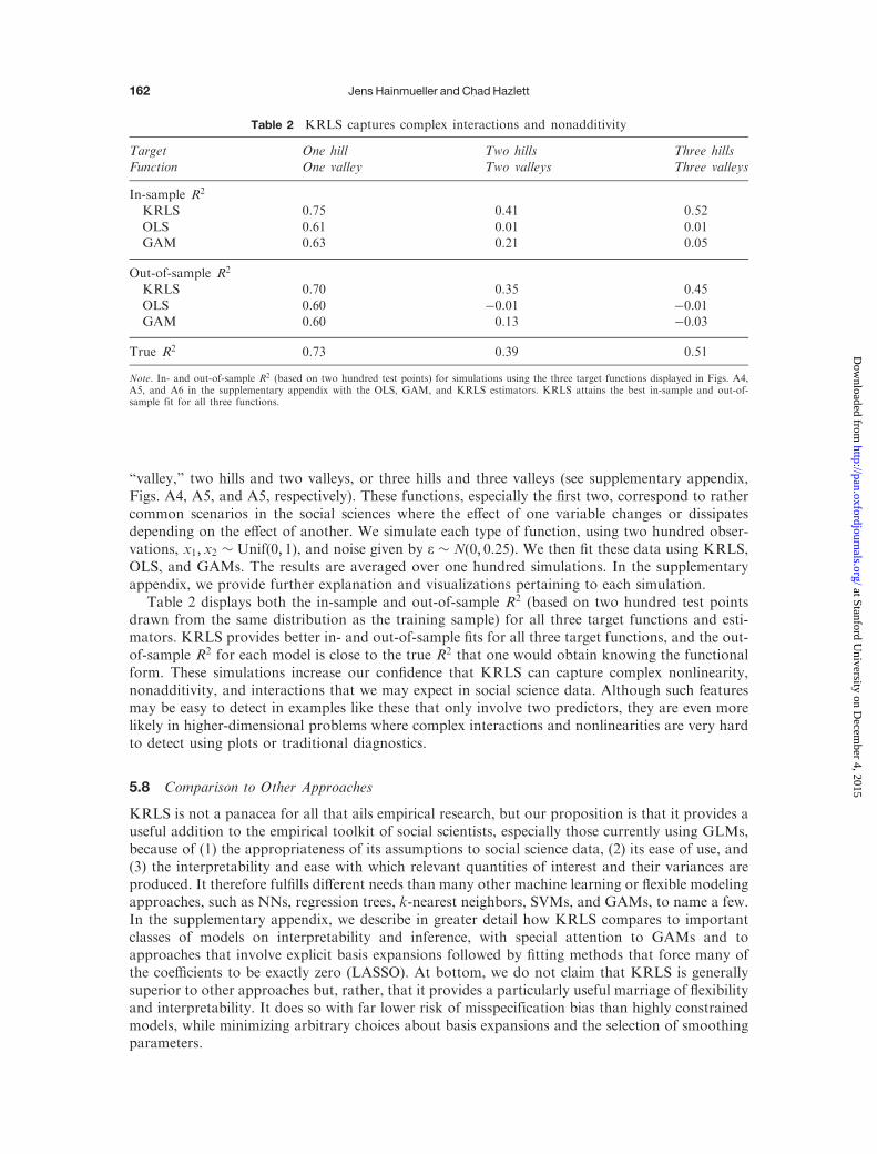
“valley,” two hills and two valleys, or three hills and three valleys (see supplementary appendix,Figs. A4, A5, and A5, respectively). These functions, especially the first two, correspond to rathercommon scenarios in the social sciences where the effect of one variable changes or dissipatesdepending on the effect of another. We simulate each type of function, using two hundred obser-vations, x1, x2 � Unifð0, 1Þ, and noise given by e � Nð0, 0:25Þ. We then fit these data using KRLS,OLS, and GAMs. The results are averaged over one hundred simulations. In the supplementaryappendix, we provide further explanation and visualizations pertaining to each simulation.

Table 2 displays both the in-sample and out-of-sample R2 (based on two hundred test pointsdrawn from the same distribution as the training sample) for all three target functions and esti-mators. KRLS provides better in- and out-of-sample fits for all three target functions, and the out-of-sample R2 for each model is close to the true R2 that one would obtain knowing the functionalform. These simulations increase our confidence that KRLS can capture complex nonlinearity,nonadditivity, and interactions that we may expect in social science data. Although such featuresmay be easy to detect in examples like these that only involve two predictors, they are even morelikely in higher-dimensional problems where complex interactions and nonlinearities are very hardto detect using plots or traditional diagnostics.

5.8 Comparison to Other Approaches

KRLS is not a panacea for all that ails empirical research, but our proposition is that it provides auseful addition to the empirical toolkit of social scientists, especially those currently using GLMs,because of (1) the appropriateness of its assumptions to social science data, (2) its ease of use, and(3) the interpretability and ease with which relevant quantities of interest and their variances areproduced. It therefore fulfills different needs than many other machine learning or flexible modelingapproaches, such as NNs, regression trees, k-nearest neighbors, SVMs, and GAMs, to name a few.In the supplementary appendix, we describe in greater detail how KRLS compares to importantclasses of models on interpretability and inference, with special attention to GAMs and toapproaches that involve explicit basis expansions followed by fitting methods that force many ofthe coefficients to be exactly zero (LASSO). At bottom, we do not claim that KRLS is generallysuperior to other approaches but, rather, that it provides a particularly useful marriage of flexibilityand interpretability. It does so with far lower risk of misspecification bias than highly constrainedmodels, while minimizing arbitrary choices about basis expansions and the selection of smoothingparameters.

Table 2 KRLS captures complex interactions and nonadditivity

Target One hill Two hills Three hillsFunction One valley Two valleys Three valleys

In-sample R2

KRLS 0.75 0.41 0.52

OLS 0.61 0.01 0.01GAM 0.63 0.21 0.05

Out-of-sample R2

KRLS 0.70 0.35 0.45

OLS 0.60 �0.01 �0.01GAM 0.60 0.13 �0.03

True R2 0.73 0.39 0.51

Note. In- and out-of-sample R2 (based on two hundred test points) for simulations using the three target functions displayed in Figs. A4,A5, and A6 in the supplementary appendix with the OLS, GAM, and KRLS estimators. KRLS attains the best in-sample and out-of-sample fit for all three functions.

Jens Hainmueller and Chad Hazlett162

at Stanford University on D

ecember 4, 2015

http://pan.oxfordjournals.org/D

ownloaded from

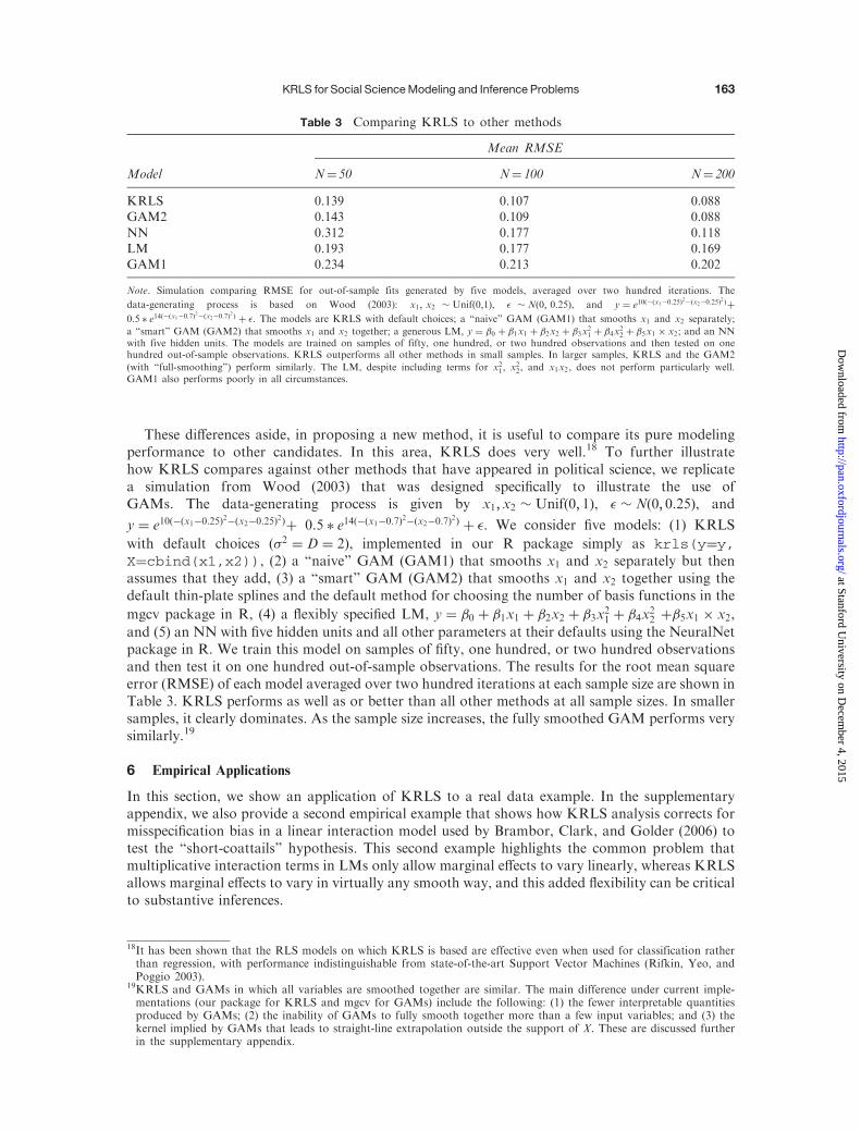
These differences aside, in proposing a new method, it is useful to compare its pure modelingperformance to other candidates. In this area, KRLS does very well.18 To further illustratehow KRLS compares against other methods that have appeared in political science, we replicatea simulation from Wood (2003) that was designed specifically to illustrate the use ofGAMs. The data-generating process is given by x1,x2 � Unifð0, 1Þ, � Nð0, 0:25Þ, and

y ¼ e10ð�ðx1�0:25Þ2�ðx2�0:25Þ

2Þþ 0:5 e14ð�ðx1�0:7Þ

2�ðx2�0:7Þ

2Þ þ . We consider five models: (1) KRLS

with default choices (�2 ¼ D ¼ 2), implemented in our R package simply as krls(y¼y,X¼cbind(x1,x2)), (2) a “naive” GAM (GAM1) that smooths x1 and x2 separately but thenassumes that they add, (3) a “smart” GAM (GAM2) that smooths x1 and x2 together using thedefault thin-plate splines and the default method for choosing the number of basis functions in the

mgcv package in R, (4) a flexibly specified LM, y ¼ �0 þ �1x1 þ �2x2 þ �3x21 þ �4x

22 þ�5x1 � x2,

and (5) an NN with five hidden units and all other parameters at their defaults using the NeuralNetpackage in R. We train this model on samples of fifty, one hundred, or two hundred observationsand then test it on one hundred out-of-sample observations. The results for the root mean squareerror (RMSE) of each model averaged over two hundred iterations at each sample size are shown inTable 3. KRLS performs as well as or better than all other methods at all sample sizes. In smallersamples, it clearly dominates. As the sample size increases, the fully smoothed GAM performs verysimilarly.19

6 Empirical Applications

In this section, we show an application of KRLS to a real data example. In the supplementaryappendix, we also provide a second empirical example that shows how KRLS analysis corrects formisspecification bias in a linear interaction model used by Brambor, Clark, and Golder (2006) totest the “short-coattails” hypothesis. This second example highlights the common problem thatmultiplicative interaction terms in LMs only allow marginal effects to vary linearly, whereas KRLSallows marginal effects to vary in virtually any smooth way, and this added flexibility can be criticalto substantive inferences.

Table 3 Comparing KRLS to other methods

Model

Mean RMSE

N¼ 50 N¼ 100 N¼ 200

KRLS 0.139 0.107 0.088GAM2 0.143 0.109 0.088

NN 0.312 0.177 0.118LM 0.193 0.177 0.169GAM1 0.234 0.213 0.202

Note. Simulation comparing RMSE for out-of-sample fits generated by five models, averaged over two hundred iterations. The

data-generating process is based on Wood (2003): x1, x2 � Unifð0,1Þ, � Nð0, 0:25Þ, and y ¼ e10ð�ðx1�0:25Þ2�ðx2�0:25Þ

2Þþ

0:5 e14ð�ðx1�0:7Þ2�ðx2�0:7Þ

2Þ þ . The models are KRLS with default choices; a “naive” GAM (GAM1) that smooths x1 and x2 separately;

a “smart” GAM (GAM2) that smooths x1 and x2 together; a generous LM, y ¼ �0 þ �1x1 þ �2x2 þ �3x21 þ �4x

22 þ �5x1 � x2; and an NN

with five hidden units. The models are trained on samples of fifty, one hundred, or two hundred observations and then tested on onehundred out-of-sample observations. KRLS outperforms all other methods in small samples. In larger samples, KRLS and the GAM2

(with “full-smoothing”) perform similarly. The LM, despite including terms for x21, x22, and x1x2, does not perform particularly well.GAM1 also performs poorly in all circumstances.

18It has been shown that the RLS models on which KRLS is based are effective even when used for classification ratherthan regression, with performance indistinguishable from state-of-the-art Support Vector Machines (Rifkin, Yeo, andPoggio 2003).

19KRLS and GAMs in which all variables are smoothed together are similar. The main difference under current imple-mentations (our package for KRLS and mgcv for GAMs) include the following: (1) the fewer interpretable quantitiesproduced by GAMs; (2) the inability of GAMs to fully smooth together more than a few input variables; and (3) thekernel implied by GAMs that leads to straight-line extrapolation outside the support of X. These are discussed furtherin the supplementary appendix.

KRLS for Social Science Modeling and Inference Problems 163

at Stanford University on D

ecember 4, 2015

http://pan.oxfordjournals.org/D

ownloaded from

6.1 Predicting Genocide

In a widely cited article, Harff (2003) examines data from 126 political instability events (i.e.,internal wars and regime changes away from democracy) to determine which factors can be usedto predict whether a state will commit genocide.20 Harff proposes a “structural model of genocide”where a dummy for genocide onset (onset) is regressed on two continuous variables, prior upheaval(summed years of prior instability events in the past fifteen years) and trade openness (imports andexports as a fraction of gross domestic product [GDP] in logs), and four dummy variables thatcapture whether the state is an autocracy, had a prior genocide, and whether the ruling elite has anideological character and/or an ethnic character.21 The first column in Table 4 replicates the originalspecification, using a linear probability model (LPM) in place of the original logit. We use the LPMhere because this allows more direct comparison to the KRLS results. However, the substantiveresults of the LPM are virtually identical to those of the logit in terms of magnitude and statisticalsignificance. The next four columns on the left present the replication results from the KRLSestimator. We report first differences for all the binary predictor variables, as described above.

The analysis yields several lessons. First, the in-sample R2 from the original logit model andKRLS are very similar (32% versus 34%), but KRLS dominates in terms of its receiver operatorcurve (ROC) for predicting genocide, with statistically significantly more area under the curve(p < 0:03). It is reassuring that KRLS performs better (at least in-sample) than the original logitmodel even though, as Harff reports, her final specification was selected after an extensive searchthrough a large number of models. Moreover, this added predictive power does not require anyhuman specification search; the researcher simply passes the predictor matrix to KRLS, whichlearns the functional form from the data, and this improves empirical performance and reducesarbitrariness in selecting a particular specification.

Second, the average marginal effects reported by KRLS (shown in the second column) are all ofreasonable size and tend to be in the same direction as but somewhat smaller than the estimatesfrom the linear probability model. We also see some important differences. The LPM model (andthe original logit) shows a significant effect of prior upheaval, with an increase of one standarddeviation corresponding to a ten-percentage-point increase in the probability of genocide onset,which corresponds to a 37% increase over the baseline probability. This sizable “effect” completelyvanishes in the KRLS model, which yields an average marginal effect of zero that is also highlyinsignificant. This sharply different finding is confirmed when we look beyond the average marginaleffect. Recall that the average marginal effects, although a useful summary tool especially tocompare to GLMs, are only summaries and can hide interesting heterogeneity in the actualmarginal effects across the covariate space. To examine the effect heterogeneity, the next threecolumns on the left in Table 4 show the quartiles of the distribution of pointwise marginaleffects for each input variable. Figure 5 also plots histograms to visualize the distributions. Wesee that the effect of prior upheaval is essentially zero at every point.

What explains this difference in marginal effect estimates? It turns out that the significant effectin the LPM model is an artifact of misspecification bias. The variable prior upheaval is stronglyright-skewed and, when logged to make it more appropriate for linear or logistic regression, the“effect” disappears entirely. This change in results emphasizes the risk of mistaken inference due tomisspecification under GLMs and its potential impact on interpretation. Note that this difference inresults is by no means trivial substantively. In fact, Harff (2003) argues that prior upheaval is “thenecessary precondition for genocide and politicide” and “a concept that captures the essence of thestructural crises and societal pressures that are preconditions for authorities’ efforts to eliminateentire groups.” Harff (2003) goes on to explain two mechanisms by which this variable matters anddraws policy conclusions from it. However, as the KRLS results show, this “important finding”

20The American Political Science Association lists this article as the 15th most downloaded paper in the AmericanPolitical Science Review. According to Google Scholar, this article has been cited 310 times.

21See Harff (2003) for details. Notice that Harff dichotomized a number of continuous variables (such as the polity score),which discards valuable information. With KRLS, one could instead use the original continuous variables unless therewas a strong reason to code dummies. In fact, tests confirm that using the original continuous variables with KRLSresults in a more predictive model.

Jens Hainmueller and Chad Hazlett164

at Stanford University on D

ecember 4, 2015

http://pan.oxfordjournals.org/D

ownloaded from

Distributions of pointwise marginal effects

marginal effect

Per

cent

of T

otal

−0.2 0.0 0.2

PriorUpheaval

−0.2 0.0 0.2

PriorGen

−0.2 0.0 0.2

IdeologicalChar

0

5

10

15

20

25

30

0

5

10

15

20

25

30

Autoc EthnicChar TradeOpen

Fig. 5 Effect heterogeneity in Harff data. Histograms of pointwise marginal effects based on KRLS fit tothe Harff data (Model 2 in Table 4).

Table 4 Predictors of genocide onset: OLS versus KRLS

Estimator OLS KRLS

@y/@xij

� Average 1st Qu. Median 3rd Qu.

Prior upheaval 0.009* 0.002 �0.001 0.002 0.004(0.004) (0.003)

Prior genocide 0.263* 0.190* 0.137 0.232 0.266(0.119) (0.075)

Ideological char. of elite 0.152 0.129 0.086 0.136 0.186(0.084) (0.076)

Autocracy 0.160* 0.122 0.092 0.114 0.136(0.077) (0.068)

Ethnic char. of elite 0.120 0.052 0.012 0.046 0.078

(0.083) (0.077)Trade openness (log) �0.172* �0.093* �0.142 �0.073 �0.048

(0.057) (0.035)

Intercept 0.659(0.217)

Note. Replication of the “structural model of genocide” by Harff (2003). Marginal effects of predictors from OLS regression and KRLSregression with standard errors in parentheses. For KRLS, the table shows the average of the pointwise derivative as well as the quartilesof their distribution to examine the effect heterogeneity. The dependent variable is a binary indicator for genocide onsets. N¼ 126.*p< 0.05.

KRLS for Social Science Modeling and Inference Problems 165

at Stanford University on D

ecember 4, 2015

http://pan.oxfordjournals.org/D

ownloaded from

readily disappears when the model accounts for the skew. This showcases the general problem that

misspecification bias is often difficult to avoid in typical political science data, even for experienced

researchers who publish in top journals and engage in various model diagnostics and specification

searches. It also highlights the advantages of a more flexible approach such as KRLS, which avoids

misspecification bias while yielding marginal effects estimates that are as easy to interpret as

coefficient estimates from a regression model and also make richer interpretation possible.Third, although using KRLS as a robustness test of more rigid models can thus be valu-

able, working in a much richer model space also permits exploration of effect heterogeneity,

including interactions. In Fig. 5 we see that for several variables, such as autocracy and ideo-

logical character, the marginal effect lies to the same side of zero at almost every point,

indicating that these variables have marginal effects in the same direction regardless of their

level or the levels of other variables. We also see that some variables show little variation in

marginal effects, such as prior upheaval, whereas others show more substantial variation, such as

prior genocide.For example, the marginal effects (measured as first-differences) of ethnic character and ideolo-

gical character are mostly positive, but both show variation from approximately zero to twenty

percentage points. A suggestive summary of how these marginal effects relate to each observed

covariate can be provided by regressing the estimates of the pointwise marginal effects@ onset

@ ideological character or @onset@ ethnic character on the covariates.22 Both regressions reveal a strong negative

relationship of the level of trade openness on these marginal effects. To give substantive interpret-

ation to the results, we find that having an ethnic character to the ruling elite is associated with

a three-percentage-point higher probability of genocide for countries in the highest quartile of

trade openness, but a nine-percentage-point higher probability in the highest quartile of trade

openness. Ideological character is associated with a nine-percentage-point higher risk of genocide

for the countries in the top quartile of trade openness, but an eighteen-percentage-point higher risk

among those in the first quartile of trade openness. These findings, while associational only, are

consistent with theoretical expectations, but would be easily missed in models that do not allow

sufficient flexibility.In addition, the marginal effects of prior genocide are very widely dispersed. We find that the

marginal effects of prior genocide and ideological character are strongly related: when one is high,

the marginal effect of the other is lessened on average. For example, the marginal effect of ideolo-

gical character is eighteen percentage points higher when prior genocide is equal to zero.

Correspondingly, the marginal effect of prior genocide is twenty-one percentage points higher

when ideological character is equal to zero. This is characteristic of a sub-additive relationship,

in which either prior genocide or ideological character signals a higher risk of genocide, but once

one of them is known, the marginal effect of the other is negligible.23 In contrast, the marginal

effects of ethnic character—and every other variable besides ideological character—changes by little

as a function of prior genocide.This brief example demonstrates that KRLS is appropriate and effective in dealing

with real-world data even in relatively small data sets. KRLS offers much more flexibility

than GLMs and guards against misspecification bias that can result in incorrect substantive

22This approach is helpful to identify nonlinearities and interaction effects. For each variable, take the pointwise partialderivatives (or first-differences) modeled by KRLS and regress them on all original independent variables to see which

of them help explain the marginal effects. For example, if @y@xðaÞ

is found to be well-explained by xðaÞ itself, then this

suggests a nonlinearity in xðaÞ (because the derivative changes with the level of the same variable). Likewise, if @y@xðaÞ

is

well-explained by another variable, xðbÞ, this suggests an interaction effect (the marginal effect of one variable, xðaÞ,

depends on the level of another, xðbÞÞ.23In addition to theoretically plausible reasons why these effects are sub-additive, this relationship may be partly due to expost facto coding of the variables: once a prior genocide has occurred, it becomes easier to classify a government ashaving an ideological character, since it has demonstrated a willingness to kill civilians, possibly even stating an ideo-logical aim as justification. Thus, in the absence of prior genocide, coding a country as having ideological character isinformative of genocide risk, whereas it adds less after prior genocide has been observed.

Jens Hainmueller and Chad Hazlett166

at Stanford University on D

ecember 4, 2015

http://pan.oxfordjournals.org/D

ownloaded from

inferences. It is also straightforward to interpret the KRLS results in ways that are familiar toresearchers from GLMs.

7 Conclusion

To date, it has been difficult to find user-friendly approaches that avoid the dangers of

misspecification while also conveniently generating quantities of interest that are as interpretableand appealing as the coefficients from GLMs. We argue that KRLS represents a particularly usefulmarriage of flexibility and interpretability, especially for current GLM users looking for more

powerful modeling approaches. It allows investigators to easily model nonlinear and nonadditiveeffects and reduce misspecification bias and still produce quantities of interest that enable “simple”interpretations (similar to those allowed by GLMs) and, if desired, more nuanced interpretations

that examine nonconstant marginal effects.Although interpretable quantities can be derived from almost any flexible modeling approach

with sufficient knowledge, computational power, and time, constructing such estimates for manymethods is inconvenient at best and computationally infeasible in some cases. Moreover, conduct-

ing inference over derived quantities of interest multiplies the problem. KRLS belongs to a class ofmodels, those producing continuously differentiable solution surfaces with closed-form expressions,that makes such interpretation feasible and fast. All the interpretational and inferential quantities

are produced by a single run of the model, and the model does not require user input regardingfunctional form or parameter settings, improving falsifiability.

We have illustrated how KRLS accomplishes this improved trade-off between flexibility andinterpretability by starting from a different set of assumptions altogether: rather than assume that

the target function is well-fitted by a linear combination of the original regressors, it is insteadmodeled in an N-dimensional space using information about similarity to each observation, butwith a preference for less complicated functions, improving stability and efficiency. Since KRLS is a

global method (i.e., the estimate at each point uses information from all other points), it is lesssusceptible to the curse of dimensionality than purely local methods such as k-nearest neighborsand matching.

We have established a number of desirable properties of this technique. First, it allows compu-

tationally tractable, closed-form solutions for many quantities, including E ½yjX�, the variance ofthis estimator, the pointwise partial derivatives with respect to each variable, the sample averagepartial derivatives, and their variances. We have also shown that it is unbiased, consistent,

and asymptotically normal. Simulations have demonstrated the performance of this method,even with small samples and high-dimensional spaces. They have also shown that even whenthe true data-generating process is linear, the KRLS estimate of the average partial derivative

is not much less efficient than the analogous OLS coefficient and far more robust to badleverage points.

We believe that KRLS is broadly useful whenever investigators are unsure of the functional formin regression and classification problems. This may include model-fitting problems such as predic-

tion tasks, propensity score estimation, or any case where a conditional expectation function mustbe acquired and rigid functional forms risk missing important variation. The method’s interpret-ability also makes it suitable for both exploratory analyses of marginal effects and causal inference

problems in which accurate conditioning on a set of covariates is required to achieve a reliablecausal estimate. Relatedly, using KRLS as a specification check for more rigid methods can also bevery useful.

However, there remains considerable room for further research. Our hope is that the

approach provided here and in our companion software will allow more researchers to beginusing KRLS or methods like it; only when tested by a larger community of scholars will we beable to determine the method’s true usefulness. Specific research tasks remain as well. Due to the

memory demands of working with an N�N matrix, the practical limit on N for most users iscurrently in the tens of thousands. Work on resolving this constraint would be useful. In addition,the most effective methods for choosing � and �2 are still relatively open questions, and it would be

KRLS for Social Science Modeling and Inference Problems 167

at Stanford University on D

ecember 4, 2015

http://pan.oxfordjournals.org/D

ownloaded from

useful to develop heteroscedasticity-, autocorrelation-, and cluster-robust estimators for standard

errors.

References

Beck, N., G. King, and L. Zeng. 2000. Improving quantitative studies of international conflict: A conjecture. American

Political Science Review 94:21–36.

Brambor, T., W. Clark, and M. Golder. 2006. Understanding interaction models: Improving empirical analyses. Political

Analysis 14(1):63–82.

De Vito, E., A. Caponnetto, and L. Rosasco. 2005. Model selection for regularized least-squares algorithm in learning

theory. Foundations of Computational Mathematics 5(1):59–85.

Evgeniou, T., M. Pontil, and T. Poggio. 2000. Regularization networks and support vector machines. Advances in

Computational Mathematics 13(1):1–50.

Friedrich, R. J. 1982. In defense of multiplicative terms in multiple regression equations. American Journal of Political

Science 26(4):797–833.

Golub, G. H., M. Heath, and G. Wahba. 1979. Generalized cross-validation as a method for choosing a good ridge

parameter. Technometrics 21(2):215–23.

Harff, B. 2003. No lessons learned from the Holocaust? Assessing risks of genocide and political mass murder since 1955.

American Political Science Review 97(1):57–73.

Hastie, T., R. Tibshirani, and J. Friedman. 2009. The elements of statistical learning: Data mining, inference, and

prediction. 2nd ed. New York, NY: Springer.

Jackson, J. E. 1991. Estimation of models with variable coefficients. Political Analysis 3(1):27–49.

Kimeldorf, G., and G. Wahba. 1970. A correspondence between Bayesian estimation on stochastic processes and

smoothing by splines. Annals of Mathematical Statistics 41(2):495–502.

King, G., and L. Zeng. 2006. The dangers of extreme counterfactuals. Political Analysis 14(2):131–59.

Rifkin, R. M., and R. A. Lippert. 2007. Notes on regularized least squares. Technical report, MIT Computer Science and

Artificial Intelligence Laboratory.

Rifkin, R., G. Yeo, and T. Poggio. 2003. Regularized least-squares classification. Nato Science Series Sub Series III

Computer and Systems Sciences 190:131–54.

Saunders, C., A. Gammerman, and V. Vovk. 1998. Ridge regression learning algorithm in dual variables. In Proceedings

of the 15th International Conference on Machine Learning. Volume 19980, 515–21. San Francisco, CA: Morgan

Kaufmann.

Scholkopf, B., and A. Smola. 2002. Learning with kernels: Support vector machines, regularization, optimization, and

beyond. Cambridge, MA: MIT Press.

Tychonoff, A. N. 1963. Solution of incorrectly formulated problems and the regularization method. Doklady Akademii

Nauk SSSR 151:501–4. Translated in Soviet Mathematics 4:1035–8.

Wood, S. N. 2003. Thin plate regression splines. Journal of the Royal Statistical Society: Series B (Statistical

Methodology) 65(1):95–114.

Jens Hainmueller and Chad Hazlett168

at Stanford University on D

ecember 4, 2015

http://pan.oxfordjournals.org/D

ownloaded from