Estimation of reference evapotranspiration using machine

AIMS Geosciences, 7(3): 268–290.

DOI: 10.3934/geosci.2021016

Received: 28 May 2021

Accepted: 05 July 2021

Published: 07 July 2021

http://www.aimspress.com/journal/geosciences

Research article

Estimation of reference evapotranspiration using machine learning

models with limited data

Adeeba Ayaz1, Maddu Rajesh1, Shailesh Kumar Singh2,* and Shaik Rehana1

1 Lab for Spatial Informatics, International Institute of Information Technology, Hyderabad, India 2 National Institute of Water & Atmospheric Research Ltd (NIWA), New Zealand

* Correspondence: Email: [email protected]; Tel: 6433438053.

Abstract: Reference Evapotranspiration (ET0) is a complex hydrological variable defined by various climatic variables affecting water and energy balances and critical factors for crop water requirements and irrigation scheduling. Conventionally ET0 is calculated by various empirical methods based on rigorous climatic data. However, there are many places where various climatic data may not available for ET0 estimation. The objective of this study is to evaluate different machine learning (ML) techniques to estimate ET0 with minimal climatic inputs. In this study, FAO-56 Penman-Monteith model was considered as the standard model and different ML models based on A Long short-term memory neural networks (LSTM), Gradient Boosting Regressor (GBR), Random Forest (RF) and Support Vector Regression (SVR) were developed to estimate ET0 with climatic variables as input parameters. These models were evaluated in two different climatic regions, Hyderabad in India and Waipara in New Zealand. The results indicated that 99 % accuracy could be achieved with all climatic input, whereas accuracy drops to 86% with fewer data. LSTM model performed better than other ML models with all input combinations at both the stations, followed by SVR and RF. Both LSTM and SVR models have been noted as the most robust ML models for estimating ET0 with minimal climate data. Even though the excellent performance can be achievable when all input variables are used, the study, however, found that even a three-parameter combination (Temperature, Wind Speed and Relative Humidity values) or two-parameter combination (Temperature and Relative Humidity, Temperature and Wind Speed) can also be promising in ET0 estimation. The presented study will help to estimate ET0 for data scare regions, which is vital for agricultural water management in semi-arid climates.

269

AIMS Geosciences Volume 7, Issue 3, 268–290.

Keywords: evapotranspiration; gradient boosting regressor; long short-term memory; penman-monteith; random forest; support vector regression

1. Introduction

Evapotranspiration (ET0) is the process wherein water starting from an expansive scope of sources is moved from the soil and vegetation layer to the atmosphere. Water loss from a vegetative surface through the consolidated cycles of plant transpiration and soil and atmospheric evaporation. It is proportional to and frequently alluded to as consumptive use. The best possible assessment of ET0 is an essential issue in food security research, land management frameworks, contamination recognition, irrigation planning and scheduling, hydrological balance studies, and watershed hydrology. Knowledge of ET0 is essential while managing water resources and management problems, such as the stipulation of the water for irrigation, agriculture, drinking and industrial use, or water reserve management [1]. ET0 also offers potential advantages for irrigation management. Hence, the exact calculation of ET0 is fundamental in improving irrigation efficiency, water reuse and seepage control [2–3]

The laws of mass or energy preservation or both were always associated with the evaluation of ET0. In recent years, various ET0 estimating procedures and modelling methods are available in the literature. ET0 assessments can be performed utilizing distinctive exploratory methods, for example, the leaf (porometer), an individual plant (for example, lysimeter), at the field scale (for example, field water balance, Bowen proportion, scintillometer) and landscape scale (for instance eddy correlation and catchment water balance) [4]. However, some of these techniques are not practical for long haul estimation over a vast region because of regular maintenance and significant expense [4,5] referenced that the main factor influencing ET0 is climatic variables so that ET0 can be surveyed by experimental and semi-experimental equations from meteorological data. Numerous strategies dependent on climatic data have already been proposed. However, the Food and Agriculture Organization of the United Nations (FAO) suggested that the (FAO56-PM) be utilized as the standard method to assess ET0 [6]. This equation has picked up the parcel of acknowledgment and utilized worldwide for benchmark evapotranspiration assessments [6].

The Penman-Monteith equation has two critical advantages. First, it can be used in a wide variety of environments and climate scenarios without the need for any local calibrations because of its physical basis. Second, it is a well-documented method that has been validated using lysimeters under a wide range of climate conditions [7]. The main drawback of this equation is that it requires loads of climatic factors, including Temperature, Wind Speed, Solar Radiation, and Relative Humidity, are required, that are unavailable in many regions. In some cases, these factors are incomplete or not accessible in a given meteorological station, particularly in developing nations [8]. Consequently, it is fundamental to build up a more precise methodology that could compute ET0 with high accuracy, particularly in data-scarce regions. Potential Evapotranspiration (PET), Reference Evapotranspiration (ET0), and Actual Evapotranspiration (AET) are the terms that are commonly utilized in the literature to characterize evapotranspiration. The PET was characterized by [9] as the maximal water amount moved to the climate, from a vegetation spread in a condition of full physiological activity and unlimited water and supplement accessibility [1]. The reference evapotranspiration idea was

270


presented by designers and specialists of hydrology in the last part of the 1970s and mid-80s to stay away from the ambiguity that existed in the definition of potential evapotranspiration [10]. Reference Evapotranspiration is the ET0 rate not highest from the extended area entirely covered by grasses of 12–15 cm high completely covering the ground. It is an abundant soil moisture substance [11]. PET is the ET from a vegetated surface with an infinite supply of water. However, because PET is still dependent on vegetation-specific characteristics (as previously mentioned) rather than solely meteorological variables, there was a determined need for a reference surface that was independent of vegetation and soil characteristics [5,11] This reference surface would allow for the analysis of the “atmospheric evaporative demand”, leaving only meteorological factors to be considered [6,12].

This simplifies ET calculation by generating a single surface against which other surfaces (e.g., different vegetation types) can be compared. Furthermore, the use of such an ET term would eliminate the need to vary the ET equation at various stages of vegetative growth [6]. This new type of ET, referred to as reference 14 evapotranspiration (ET0), simply “expresses the evaporating power of the atmosphere at a specific location and time of year” [6]. ET0 can also be viewed as a subset of PET in which the transpiring vegetation has been specifically defined. Explicit standardized equations and procedures are being suggested for reference evapotranspiration estimates and are typically modeled utilizing climate data and algorithms that depict surface vitality and aerodynamic qualities of the vegetation.

Several empirical models for assessing ET0 with limited data can also be categorized as mass exchange-based, temperature-based, radiation-based, pan-evaporation based, and combination type [8], inferred a model for measuring evaporation from open surfaces by the mix of vitality offset with mass exchange techniques. [13] proposed the radiation-based Priestley-Taylor model, a rearrangement of the Penman model. [14] proposed the temperature-based Hargreaves model, which was perhaps the least complicated strategy. Eleven temperature-based ET0 techniques were evaluated for assessing ET0, and were discovered that the Hargreaves method gave an excellent performance in arid, semi-arid, temperate, cold, and polar atmospheres [10].

Because of the reliance on different climatic components, several researchers considered the calculation of ET0 as a complicated non-direct regression process and have progressed the assessment of ET0 models using computing procedures, for example, prepared Artificial Intelligence (AI), Machine learning models, and statistical regression approaches. [15] detailed gene expression programming (GEP), with its capacity to represent algebraic equations, to be a reliable procedure for modelling the decadal ET0 of six districts in Burkina Faso. [16] found a versatile neuro-fuzzy inference system (ANFIS) that outperformed Artificial neural networks (ANN) in modelling the monthly mean ET0. Additionally, [17] evaluated the ANN, GEP, and ANFIS-grid partitioning (ANFIS-GP) models to display monthly ET0, discovered that the ANFIS-GP model performed well compared to other models. [18] discovered ANN models to give more superior accuracy than GEP models in comparing GEP and ANN for modelling daily ET0. Moreover, [19], assessing week by week ET at Pali and Jodhpur, India, related the performance of ANN, least-square SVM, and extreme learning machine (ELM) approaches. The ELM gave preferable ET0 estimates over the other two models. [20] found that the ANN model gives preferred outcomes over the experimental conditions in assessing ANN’s performance and four empirical methods for demonstrating every day ET0 at the Amineto climate station in Greece. [21] assessed the ET0 in Florida, USA, utilizing M5P regression tree, SVR, and RF procedures and announced that these techniques were all prepared to model ET0 in the study area. [22] used ANFIS, feed-forward neural networks (FFNN), and SVR

271


ensemble-based models to model ET0 at 14 stations in Iran, Iraq, Libya, Turkey, and Cyprus. They found the ensemble techniques improved the performance of traditional ML models. ET0

demonstrating methods that likewise incorporate SVR and RF were applied by [15,23–26]. Assessment of the precision of regression and machine learning approaches recommends that such methodologies estimate better ET0 over empirical models, such as the [1] and [14], which utilized limited meteorological factors. [27,28] compared the performance of four atmosphere-based methods and ANNs to assess ET0 when input climatic parameters were insufficient to apply the FAO Penman-Monteith method. They inferred that ANN models performed superior to climatic techniques. In the 1st case, they have used 4 meteorological variables (T, RH, Rs and u2) as input variables. In the 2nd case, 3 variables (T, RH, and Rs), were used and in the 3rd case, 2 variables (T and RH or T and Rs), were used. [29] inspected the temperature and potential evapotranspiration pattern over the Betwa bowl, India. [30] examined the pattern of minimum and maximum temperature of yearly, monthly, winter, pre-monsoon, monsoon, and post-monsoon. Assessment of the ET0 of Punjab was done by [31] was done dependent on different machine learning models including Deep Learning-Multilayer Perceptrons (DL), Generalized Linear Model (GLM), Random Forest (RF), and Gradient-Boosting Machine (GBM) models. It was compared in predicting daily ET0 with the deep learning model’s performance and was compared with the Penman-Monteith model and found that deep learning models performed superior to the considered models for training, validation and testing sets. [32] examined the unique data-driven based regression approaches to deal with daily ET0 modelling utilizing four data-inputs, including average air temperature, average wind speed, average relative humidity, and solar radiation. Results from their examination proposed that the unique data-driven and AI models could effectively be utilized in modelling the ET0. [33] investigated Support vector regression model for large scale regression problems and investigated the performance of Support vector regression model. [34] investigated the viability of the deep learning neural network (DLNN) for estimating the ET0. The LSTM model was developed by [35] to predict the dynamic of the water table depth in five sub-areas in arid north-western China. The results showed that the LSTM model achieved the best performance among the considered feed-forward neural network and double LSTM models.

With the upcoming technology, there has been a drastic change in many industries over the globe [36], however agribusiness, being the least digitized, has also seen the development and commercialization of rural advances. Machine learning models and Deep learning models have also started to assume a significant function in everyday lives, stretching out our recognitions and capacity to adjust the earth around us, With this rising innovations the workforce which were confined to just a negligible mechanical areas are currently adding to various segments. Implementation of automation in agriculture, the weeding systems were studied using machine learning models by [37]. Correlations of direct profundities or ET0 rates with estimates from other timeframes or different areas aren't a viable method for evaluating ET0 data.ET0 profundities are firmly affected by climate and atmosphere and consequently change with time or area, therefore. Direct correlations ought to be made in the wake of normalizing the ET0 estimate or estimation utilizing reference ET0 to represent climate impacts by expressing it as a fraction of reference ET0. The current study gives a comparison of four ML based models to discover the best model for assessing daily ET0 under the state of minimal input variables in the semi-arid atmospheres in two unique areas, for example, Hyderabad, India and Waipara, New Zealand. The objectives of the current study are as per the following: (1) to develop different ML models, SVR, LSTM, RF and

272


GBR for modelling ET0 in Hyderabad and Waipara Stations (2) to assess the performance and stability of these models with different input combinations over the two stations (3) to find an appropriate approach to boost the modelling performance under the limited input factors condition.

2. Data and case study

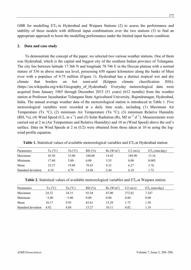
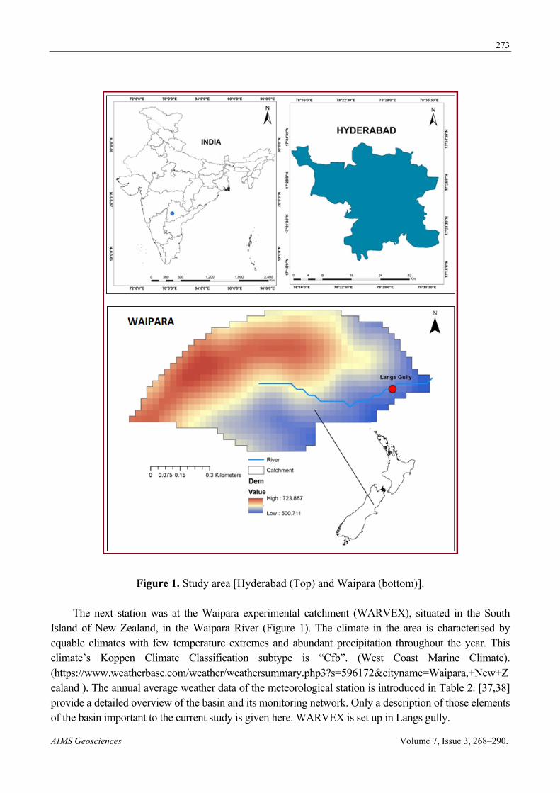
To demonstrate the concept of the paper, we selected two various weather stations. One of them was Hyderabad, which is the capital and biggest city of the southern Indian province of Telangana. The city lies between latitude 17.366 N and longitude 78.746 E in the Deccan plateau with a normal stature of 536 m above mean sea level, possessing 650 square kilometers along the banks of Musi river with a populace of 9.75 million (Figure 1). Hyderabad has a distinct tropical wet and dry climate that borders on hot semi-arid (Köppen climate classification BSh). (https://en.wikipedia.org/wiki/Geography_of_Hyderabad). Everyday meteorological data were acquired from January 1965 through December 2015 (51 years) (612 months) from the weather station at Professor Jayashankar Telangana State Agricultural University, Rajendranagar, Hyderabad, India. The annual average weather data of the meteorological station is introduced in Table 1. Five meteorological variables were recorded at a daily time scale, including (1) Maximum Air Temperature (Tx °C); (2) minimum Air Temperature (Tn °C); (3) minimum Relative Humidity (RH, %); (4) Wind Speed (U2, m s−1) and (5) Solar Radiation (Rs, MJ m−2 d−1). Measurements were carried out at 2 m (Air Temperature and Relative Humidity) and 10 m (Wind Speed) above the soil’s surface. Data on Wind Speeds at 2 m (U2) were obtained from those taken at 10 m using the log-wind profile equation.

Table 1. Statistical values of available meteorological variables and ET0 at Hyderabad station.

Parameters Tx (oC) Tn (oC) RH (%) Rs (W/m2) U2 (m/s) ET0 (mm/day)

Maximum 45.50 33.00 100.00 14.45 189.90 13.16

Minimum 17.60 5.00 6.00 3.55 0.00 0.005

Mean 32.37 19.88 78.43 9.32 6.27 3.76

Standard deviation 4.10 4.79 14.48 2.44 6.18 1.72

Table 2. Statistical values of available meteorological variables and ET0 at Waipara station.

Parameters Tx (oC) Tn (oC) RH (%) Rs (W/m2) U2 (m/s) ET0 (mm/day)

Maximum 24.32 24.15 93.54 47.00 272.82 7.247

Minimum −3.00 −3.00 0.00 0.00 0.00 0.00

Mean 10.17 9.95 65.61 15.29 1.75 1.50

Standard deviation 4.92 4.88 15.27 10.11 0.82 1.18

273


Figure 1. Study area [Hyderabad (Top) and Waipara (bottom)].

The next station was at the Waipara experimental catchment (WARVEX), situated in the South Island of New Zealand, in the Waipara River (Figure 1). The climate in the area is characterised by equable climates with few temperature extremes and abundant precipitation throughout the year. This climate’s Koppen Climate Classification subtype is “Cfb”. (West Coast Marine Climate). (https://www.weatherbase.com/weather/weathersummary.php3?s=596172&cityname=Waipara,+New+Zealand ). The annual average weather data of the meteorological station is introduced in Table 2. [37,38] provide a detailed overview of the basin and its monitoring network. Only a description of those elements of the basin important to the current study is given here. WARVEX is set up in Langs gully.

274


The catchment area of the Langs gully is 0.7 km2. The elevation varies between 500 m and 723 m above sea level. The annual rainfall varies from 500 to 1100 mm/yr. It contains a surface slope of 0.22–34 degrees with a mean slope of 17 degrees. Soils are gravelly sandy loam, depth ranges from 0.25 to 1.5 m and averages 0.5 m. Grass and exotic forests are the primary vegetation. An ephemeral stream flows approximately from late March through early November. The catchment has fairly regular frosts and occasional snow in winter. Field data from Lang gully was collected from 2010 to 2016. All data were stored in data loggers and had temporal resolutions of 10 minutes and have been aggregated to the hourly time series for this study to match the model time step.

3. Methodology

The FAO-56 Penman-Monteith model determined ET0 values are regarded as the ground truth benchmarking for training and testing the different machine learning models.

3.1. Estimation of reference evapotranspiration by FAO-56 penman-monteith method

The Penman-Monteith method on a daily time scale is calculated by

ET0 = .

. (1)

Where, ET0 = reference evapotranspiration (mm d−1), D = slope vapor pressure curve [k pa°C−1], Rn = net radiation (MJ m−2 d−1), G = soil heat flux (MJ m−2 d−1), U2 = wind speed measured at 2 m height [m s−1], (es - ea) = vapor pressure deficit for measurement at 2 m height [k Pa], T = average temperature at 2 m height (°C), 900 = coefficient for the reference crop [l J-1 Kg K d-1], g = psychrometric constant [k pa°C-1], 0.34 = wind coefficient for the reference crop [s m-1].

4. Machine learning models

In this study, four ML models were implemented for modelling the ET0 relationship of the Hyderabad and Waipara stations, namely, LSTM, GBR, SVR, and RF regressor, and a comparison was made between the models. For modelling the machine learning models 70% data was used for training and 30% data was used for testing.

4.1. Long short-term memory (LSTM)

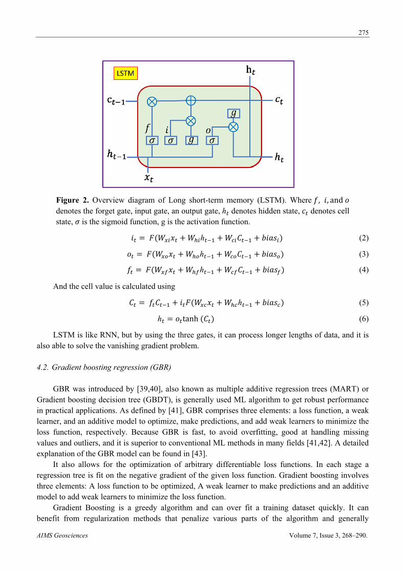
Long short-term memory neural networks are similar to Recurrent neural networks (RNN), which has the capability to learn larger data compared to normal RNNs. This is done by controlling the hidden state in LSTM and solving the vanishing gradient problem. LSTM has feedback connections. An LSTM unit has an input gate, an output gate, and a forget gate (Figure 2). LSTM calculates a gate’s values by using the previous cell value Ct-1, previously hidden values ht-1, and input xt.

275


Figure 2. Overview diagram of Long short-term memory (LSTM). Where 𝑓, 𝑖, and 𝑜 denotes the forget gate, input gate, an output gate, ℎ denotes hidden state, 𝑐 denotes cell state, 𝜎 is the sigmoid function, g is the activation function.

𝑖 𝐹 𝑊 𝑥 𝑊 ℎ 𝑊 𝐶 𝑏𝑖𝑎𝑠 (2)

𝑜 𝐹 𝑊 𝑥 𝑊 ℎ 𝑊 𝐶 𝑏𝑖𝑎𝑠 (3)

𝑓 𝐹 𝑊 𝑥 𝑊 ℎ 𝑊 𝐶 𝑏𝑖𝑎𝑠 (4)

And the cell value is calculated using

𝐶 𝑓 𝐶 𝑖 𝐹 𝑊 𝑥 𝑊 ℎ 𝑏𝑖𝑎𝑠 (5)

ℎ 𝑜 tanh 𝐶 (6)

LSTM is like RNN, but by using the three gates, it can process longer lengths of data, and it is also able to solve the vanishing gradient problem.

4.2. Gradient boosting regression (GBR)

GBR was introduced by [39,40], also known as multiple additive regression trees (MART) or Gradient boosting decision tree (GBDT), is generally used ML algorithm to get robust performance in practical applications. As defined by [41], GBR comprises three elements: a loss function, a weak learner, and an additive model to optimize, make predictions, and add weak learners to minimize the loss function, respectively. Because GBR is fast, to avoid overfitting, good at handling missing values and outliers, and it is superior to conventional ML methods in many fields [41,42]. A detailed explanation of the GBR model can be found in [43].

It also allows for the optimization of arbitrary differentiable loss functions. In each stage a regression tree is fit on the negative gradient of the given loss function. Gradient boosting involves three elements: A loss function to be optimized, A weak learner to make predictions and an additive model to add weak learners to minimize the loss function.

Gradient Boosting is a greedy algorithm and can over fit a training dataset quickly. It can benefit from regularization methods that penalize various parts of the algorithm and generally

276


improve the performance of the algorithm by reducing over fitting. There are four improvements basic gradient boosting: Tree Constraints, Shrinkage, Sampling, Penalized learning

Gradient Boosting trains many models in a gradual, additive and sequential manner. The major difference between AdaBoost and Gradient Boosting Algorithm is how the two algorithms identify the shortcomings of weak learners (e.g., decision trees). While the AdaBoost model identifies the shortcomings by using high weight data points, gradient boosting performs the same by using gradients in the loss function (y = ax + b + e, e needs a special mention as it is the error term).

The loss function is a measure indicating how good are model’s coefficients are at fitting the underlying data. A logical understanding of loss function would depend on what we are trying to optimise.

For example, if we are trying to predict the sales prices by using a regression, then the loss function would be based off the error between true and predicted house prices. Similarly, if our goal is to classify credit defaults, then the loss function would be a measure of how good our predictive model is at classifying bad loans.

One of the biggest motivations of using gradient boosting is that it allows one to optimise a user specified cost function, instead of a loss function that usually offers less control and does not essentially correspond with real world applications.

4.3. Random forest regression (RF)

RF is an ensemble technique, which is capable of both classification and regression, known as bagging. It is one of the practical algorithms for predictive analysis. In determining the final output, the principle of RF is to combine the various decision trees rather than depending on individual decision trees. RF is used for classification by majority vote and regression by an average of the single-tree method in the output generation process [40]. RF models have supervised ML approaches, which are popular in ML [43–47] and frequently used in hydrology [42,48–50]. The Sum of Squared Error (SSE) has been calculated between the observed values and the predicted values. This procedure will recursively continue until the entire data is being covered. The model can be written as:

𝑓 𝑥 𝑓 𝑥 𝑓 𝑥 𝑓 𝑥 ⋯ (7)

Where the ultimate model f is the sum of simple base models fi. Where each base regressor portion is the simple decision tree.

The basic idea behind this is to combine multiple decision trees in determining the final output rather than relying on individual decision trees.

Approach: 1. Pick at random K data points from the training set; 2. Build the decision tree associated with those K data points; 3. Choose the number Ntree of trees you want to build and repeat step 1 & 2; 4. For a new data point, make each one of your Ntree trees predict the value of Y for the data point, and assign the new data point the average across all of the predicted Y values.

Random forests or random decision forests are an ensemble learning method for classification, regression and other tasks that operate by constructing a multitude of decision trees at training time and outputting the class that is the mode of the classes (classification) or mean prediction (regression) of the individual trees. Random decision forests correct for decision trees habit of over fitting to their training set.

277


Each Decision Tree in the Extra Trees Forest is constructed from the original training sample. Then, at each test node, each tree is provided with a random sample of k features from the feature-set from which each decision tree must select the best feature to split the data based on some mathematical criteria (typically the Gini Index). This random sample of features leads to the creation of multiple de-correlated decision trees.

4.4. Support vector regression (SVR)

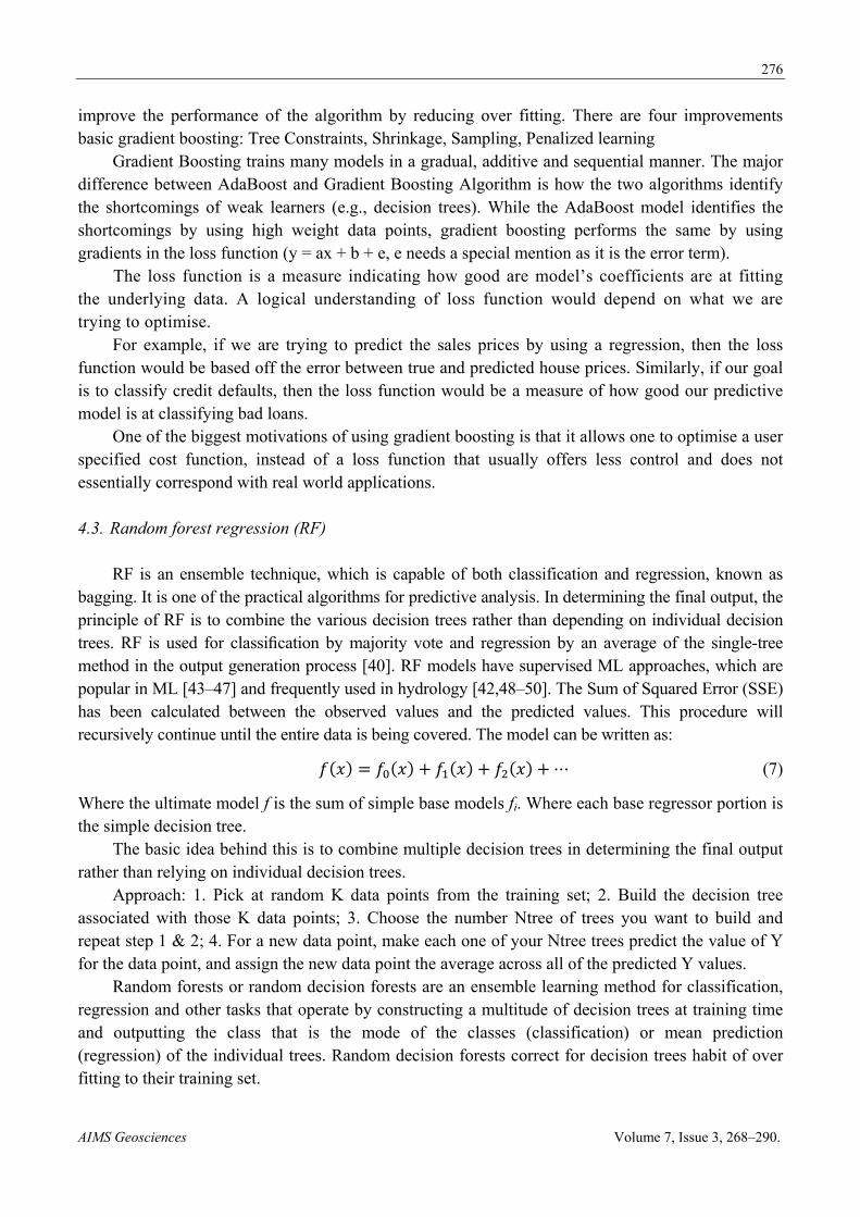
In several research studies, SVR, which is focused on systemic risk minimization to prevent overfitting [51], was adopted over ANN due to the solution’s uniqueness and globalization [52]. The SVR has been commonly used in engineering [53–55]. Its evapotranspiration applications are also quite impressive [56–58] firstly applied the SVR approach for rainfall-runoff modelling in hydrology. SVRs are today known as efficient and robust ML algorithms for predictions. When the training data of

𝑥 , 𝑦 , … … . . 𝑥 , 𝑦 with n patterns, a function 𝑓 𝑥 will be identified with the consideration of the deviation from the actually observed target variables 𝑦 for all the training data [60]. Using a non-linear mapping function φ, X will be map the input variables to a higher dimensional feature space.

Figure 3. Structure of SVR.

In simple regression we try to minimise the error rate. While in SVR we try to fit the error within a certain threshold.

Our objective when we are moving on with SVR is to basically consider the points that are within the boundary line. Our best fit line is the line hyperplane that has maximum number of points.

In the case of regression, a margin of tolerance (epsilon) is set in approximation to the SVM which would have already requested from the problem. But besides this fact, there is also a more complicated reason, the algorithm is more complicated therefore to be taken in consideration. However, the main idea is always the same: to minimize error, individualizing the hyper plane which maximizes the margin, keeping in mind that part of the error is tolerated. The goal in linear regression is to minimize the error between the prediction and data. In SVR, the goal is to make sure that the errors do not exceed the threshold.

SVRs are today known as efficient and robust ML algorithms for predictions. When the training data of 𝑥 , 𝑦 , … … . . 𝑥 , 𝑦 with n patterns, a function 𝑓 𝑥 will be identified with the

278


consideration of the deviation from the actually observed target variables 𝑦 for all the training data [60]. Using a non-linear mapping function φ, X will be mapping the input variables to a higher dimensional feature space.

𝑓 𝑥; 𝑤 𝑊, 𝜑 𝑥 𝑏 (8)

where W and b are the regression coefficients and < , > denotes the inner product. SVR uses the ∈ insensitive error to measure the error between 𝑓 𝑥 and the observed values of 𝑦.

|𝑓 𝑥; 𝑤 𝑦|∈0, 𝑖𝑓|𝑓 𝑥; 𝑤 𝑦| ∈

|𝑓 𝑥; 𝑤 𝑦| ∈, 𝑜𝑡ℎ𝑒𝑟𝑤𝑖𝑠𝑒, (9)

Using the training data of 𝑥 , 𝑦 the values of w and b are calculated by minimizing the objective function:

𝐹 |𝑓 𝑥 , 𝑤 𝑦 |∈ ||𝑤|| (10)

Where ∈ and C are the hyper-parameters. The minimization of the objective function, F, uses the Lagrange multiplier method. The ultimate regression equation with kernel function 𝐾 𝑋, 𝑋 ′ can be in the form:

𝑓 𝑋 ∑ 𝐾 𝑋, 𝑋 𝑏 (11)

Based on earlier studies [59], the kernel function RBF was chosen to measure the performance of the model for the ET0. A complete overview of the SVR method may be found in [59].

5. Model evaluation

The accuracy of the ML models was calculated using the coefficient of determination (R2) (Eq. 12), the root mean squared error (RMSE) (Eq. 13), and the mean absolute error (MAE) (Eq. 14). The equations are as follows:

𝑅 1 ∑

∑ (12)

𝑅𝑀𝑆𝐸 √𝑀𝑆𝐸∑

(13)

𝑀𝐴𝐸 ∑ 𝐸𝑇 𝐸𝑇 (14)

𝑁𝑆𝐸 1∑

∑ (15)

where 𝐸𝑇 is the simulated ET0 at time step i in mm/day; 𝐸𝑇 is the observed ET0 at time step i in mm/day; 𝐸𝑇 is the average ET0 at time step i in mm/day; n is the number of data pairs, respectively.

279


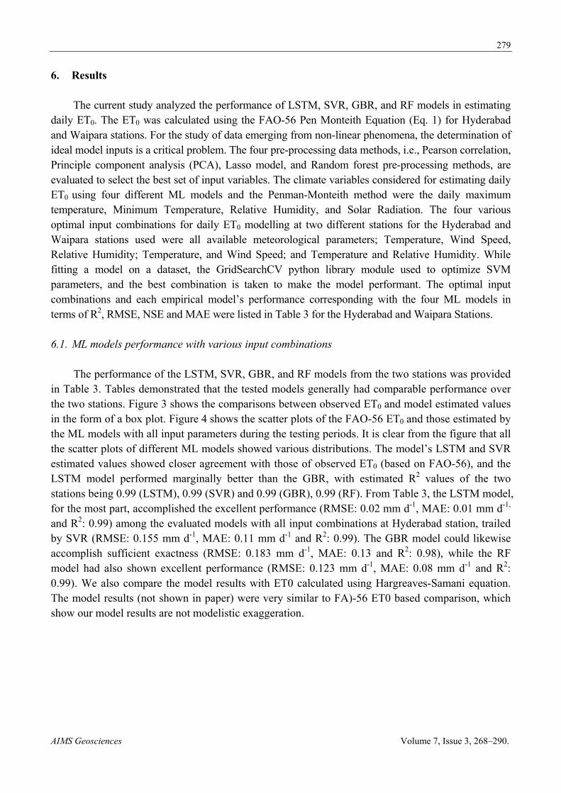
6. Results

The current study analyzed the performance of LSTM, SVR, GBR, and RF models in estimating daily ET0. The ET0 was calculated using the FAO-56 Pen Monteith Equation (Eq. 1) for Hyderabad and Waipara stations. For the study of data emerging from non-linear phenomena, the determination of ideal model inputs is a critical problem. The four pre-processing data methods, i.e., Pearson correlation, Principle component analysis (PCA), Lasso model, and Random forest pre-processing methods, are evaluated to select the best set of input variables. The climate variables considered for estimating daily ET0 using four different ML models and the Penman-Monteith method were the daily maximum temperature, Minimum Temperature, Relative Humidity, and Solar Radiation. The four various optimal input combinations for daily ET0 modelling at two different stations for the Hyderabad and Waipara stations used were all available meteorological parameters; Temperature, Wind Speed, Relative Humidity; Temperature, and Wind Speed; and Temperature and Relative Humidity. While fitting a model on a dataset, the GridSearchCV python library module used to optimize SVM parameters, and the best combination is taken to make the model performant. The optimal input combinations and each empirical model’s performance corresponding with the four ML models in terms of R2, RMSE, NSE and MAE were listed in Table 3 for the Hyderabad and Waipara Stations.

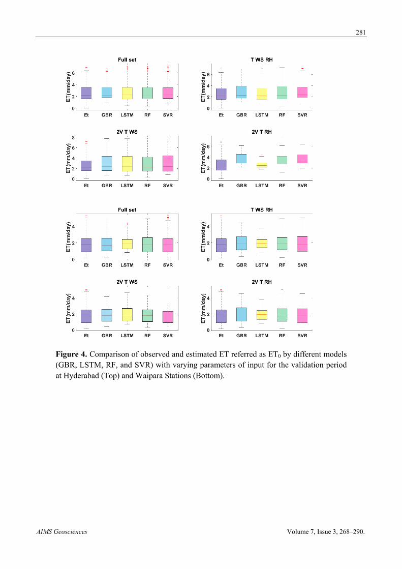
6.1. ML models performance with various input combinations

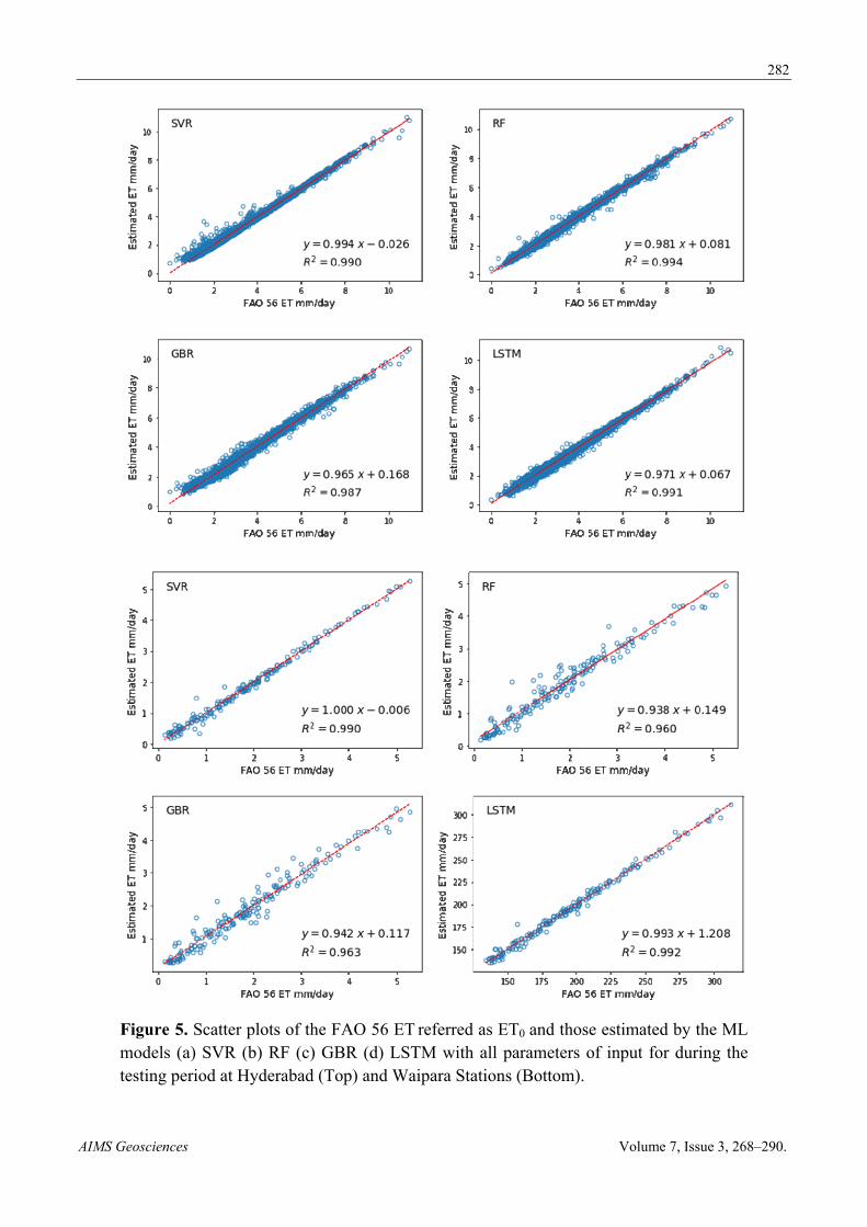
The performance of the LSTM, SVR, GBR, and RF models from the two stations was provided in Table 3. Tables demonstrated that the tested models generally had comparable performance over the two stations. Figure 3 shows the comparisons between observed ET0 and model estimated values in the form of a box plot. Figure 4 shows the scatter plots of the FAO-56 ET0 and those estimated by the ML models with all input parameters during the testing periods. It is clear from the figure that all the scatter plots of different ML models showed various distributions. The model’s LSTM and SVR estimated values showed closer agreement with those of observed ET0 (based on FAO-56), and the LSTM model performed marginally better than the GBR, with estimated R2 values of the two stations being 0.99 (LSTM), 0.99 (SVR) and 0.99 (GBR), 0.99 (RF). From Table 3, the LSTM model, for the most part, accomplished the excellent performance (RMSE: 0.02 mm d-1, MAE: 0.01 mm d-1, and R2: 0.99) among the evaluated models with all input combinations at Hyderabad station, trailed by SVR (RMSE: 0.155 mm d-1, MAE: 0.11 mm d-1 and R2: 0.99). The GBR model could likewise accomplish sufficient exactness (RMSE: 0.183 mm d-1, MAE: 0.13 and R2: 0.98), while the RF model had also shown excellent performance (RMSE: 0.123 mm d-1, MAE: 0.08 mm d-1 and R2: 0.99). We also compare the model results with ET0 calculated using Hargreaves-Samani equation. The model results (not shown in paper) were very similar to FA)-56 ET0 based comparison, which show our model results are not modelistic exaggeration.

280


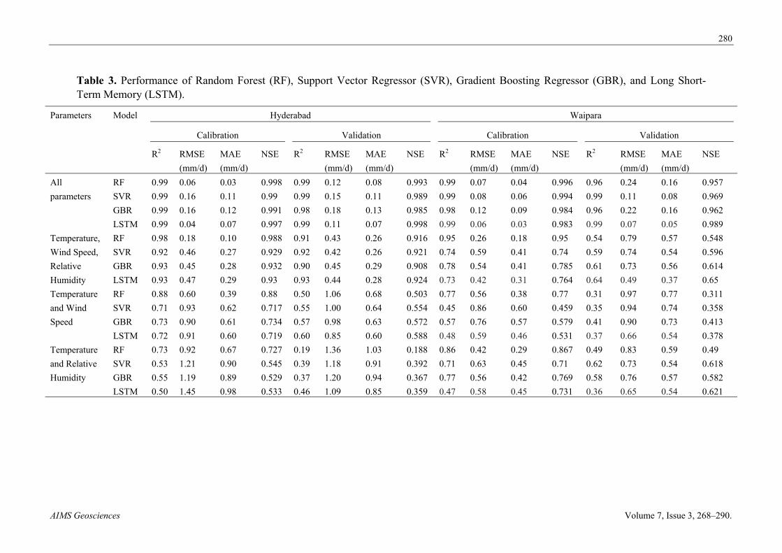
Table 3. Performance of Random Forest (RF), Support Vector Regressor (SVR), Gradient Boosting Regressor (GBR), and Long Short-Term Memory (LSTM).

Parameters Model Hyderabad Waipara

Calibration Validation Calibration Validation

R2 RMSE

(mm/d)

MAE

(mm/d)

NSE

R2 RMSE

(mm/d)

MAE

(mm/d)

NSE R2 RMSE

(mm/d)

MAE

(mm/d)

NSE

R2 RMSE

(mm/d)

MAE

(mm/d)

NSE

All

parameters

RF 0.99 0.06 0.03 0.998 0.99 0.12 0.08 0.993 0.99 0.07 0.04 0.996 0.96 0.24 0.16 0.957

SVR 0.99 0.16 0.11 0.99 0.99 0.15 0.11 0.989 0.99 0.08 0.06 0.994 0.99 0.11 0.08 0.969

GBR 0.99 0.16 0.12 0.991 0.98 0.18 0.13 0.985 0.98 0.12 0.09 0.984 0.96 0.22 0.16 0.962

LSTM 0.99 0.04 0.07 0.997 0.99 0.11 0.07 0.998 0.99 0.06 0.03 0.983 0.99 0.07 0.05 0.989

Temperature,

Wind Speed,

Relative

Humidity

RF 0.98 0.18 0.10 0.988 0.91 0.43 0.26 0.916 0.95 0.26 0.18 0.95 0.54 0.79 0.57 0.548

SVR 0.92 0.46 0.27 0.929 0.92 0.42 0.26 0.921 0.74 0.59 0.41 0.74 0.59 0.74 0.54 0.596

GBR 0.93 0.45 0.28 0.932 0.90 0.45 0.29 0.908 0.78 0.54 0.41 0.785 0.61 0.73 0.56 0.614

LSTM 0.93 0.47 0.29 0.93 0.93 0.44 0.28 0.924 0.73 0.42 0.31 0.764 0.64 0.49 0.37 0.65

Temperature

and Wind

Speed

RF 0.88 0.60 0.39 0.88 0.50 1.06 0.68 0.503 0.77 0.56 0.38 0.77 0.31 0.97 0.77 0.311

SVR 0.71 0.93 0.62 0.717 0.55 1.00 0.64 0.554 0.45 0.86 0.60 0.459 0.35 0.94 0.74 0.358

GBR 0.73 0.90 0.61 0.734 0.57 0.98 0.63 0.572 0.57 0.76 0.57 0.579 0.41 0.90 0.73 0.413

LSTM 0.72 0.91 0.60 0.719 0.60 0.85 0.60 0.588 0.48 0.59 0.46 0.531 0.37 0.66 0.54 0.378

Temperature

and Relative

Humidity

RF 0.73 0.92 0.67 0.727 0.19 1.36 1.03 0.188 0.86 0.42 0.29 0.867 0.49 0.83 0.59 0.49

SVR 0.53 1.21 0.90 0.545 0.39 1.18 0.91 0.392 0.71 0.63 0.45 0.71 0.62 0.73 0.54 0.618

GBR 0.55 1.19 0.89 0.529 0.37 1.20 0.94 0.367 0.77 0.56 0.42 0.769 0.58 0.76 0.57 0.582

LSTM 0.50 1.45 0.98 0.533 0.46 1.09 0.85 0.359 0.47 0.58 0.45 0.731 0.36 0.65 0.54 0.621

281


Figure 4. Comparison of observed and estimated ET referred as ET0 by different models (GBR, LSTM, RF, and SVR) with varying parameters of input for the validation period at Hyderabad (Top) and Waipara Stations (Bottom).

282


Figure 5. Scatter plots of the FAO 56 ET referred as ET0 and those estimated by the ML models (a) SVR (b) RF (c) GBR (d) LSTM with all parameters of input for during the testing period at Hyderabad (Top) and Waipara Stations (Bottom).

283


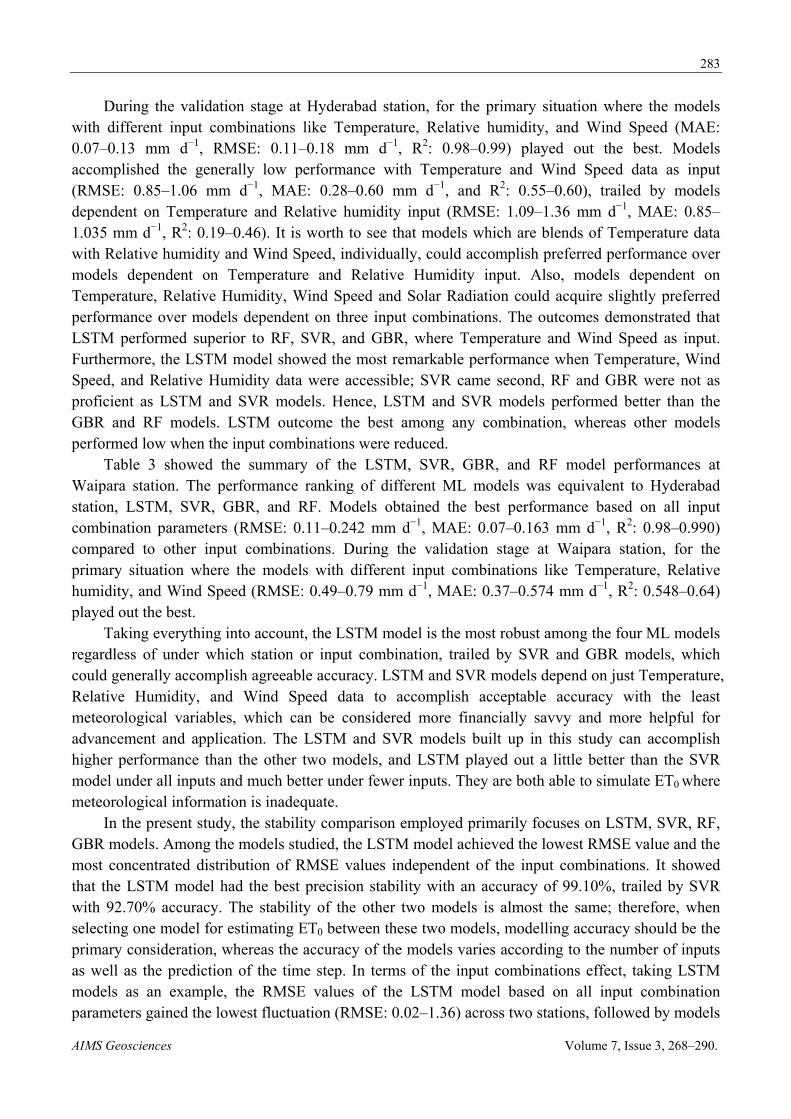
During the validation stage at Hyderabad station, for the primary situation where the models with different input combinations like Temperature, Relative humidity, and Wind Speed (MAE: 0.07–0.13 mm d−1, RMSE: 0.11–0.18 mm d−1, R2: 0.98–0.99) played out the best. Models accomplished the generally low performance with Temperature and Wind Speed data as input (RMSE: 0.85–1.06 mm d−1, MAE: 0.28–0.60 mm d−1, and R2: 0.55–0.60), trailed by models dependent on Temperature and Relative humidity input (RMSE: 1.09–1.36 mm d−1, MAE: 0.85–1.035 mm d−1, R2: 0.19–0.46). It is worth to see that models which are blends of Temperature data with Relative humidity and Wind Speed, individually, could accomplish preferred performance over models dependent on Temperature and Relative Humidity input. Also, models dependent on Temperature, Relative Humidity, Wind Speed and Solar Radiation could acquire slightly preferred performance over models dependent on three input combinations. The outcomes demonstrated that LSTM performed superior to RF, SVR, and GBR, where Temperature and Wind Speed as input. Furthermore, the LSTM model showed the most remarkable performance when Temperature, Wind Speed, and Relative Humidity data were accessible; SVR came second, RF and GBR were not as proficient as LSTM and SVR models. Hence, LSTM and SVR models performed better than the GBR and RF models. LSTM outcome the best among any combination, whereas other models performed low when the input combinations were reduced.

Table 3 showed the summary of the LSTM, SVR, GBR, and RF model performances at Waipara station. The performance ranking of different ML models was equivalent to Hyderabad station, LSTM, SVR, GBR, and RF. Models obtained the best performance based on all input combination parameters (RMSE: 0.11–0.242 mm d−1, MAE: 0.07–0.163 mm d−1, R2: 0.98–0.990) compared to other input combinations. During the validation stage at Waipara station, for the primary situation where the models with different input combinations like Temperature, Relative humidity, and Wind Speed (RMSE: 0.49–0.79 mm d−1, MAE: 0.37–0.574 mm d−1, R2: 0.548–0.64) played out the best.

Taking everything into account, the LSTM model is the most robust among the four ML models regardless of under which station or input combination, trailed by SVR and GBR models, which could generally accomplish agreeable accuracy. LSTM and SVR models depend on just Temperature, Relative Humidity, and Wind Speed data to accomplish acceptable accuracy with the least meteorological variables, which can be considered more financially savvy and more helpful for advancement and application. The LSTM and SVR models built up in this study can accomplish higher performance than the other two models, and LSTM played out a little better than the SVR model under all inputs and much better under fewer inputs. They are both able to simulate ET0 where meteorological information is inadequate.

In the present study, the stability comparison employed primarily focuses on LSTM, SVR, RF, GBR models. Among the models studied, the LSTM model achieved the lowest RMSE value and the most concentrated distribution of RMSE values independent of the input combinations. It showed that the LSTM model had the best precision stability with an accuracy of 99.10%, trailed by SVR with 92.70% accuracy. The stability of the other two models is almost the same; therefore, when selecting one model for estimating ET0 between these two models, modelling accuracy should be the primary consideration, whereas the accuracy of the models varies according to the number of inputs as well as the prediction of the time step. In terms of the input combinations effect, taking LSTM models as an example, the RMSE values of the LSTM model based on all input combination parameters gained the lowest fluctuation (RMSE: 0.02–1.36) across two stations, followed by models

284


based on Temperature, Wind Speed, Relative Humidity; Temperature, Relative Humidity; Temperature, Wind Speed. It’s also worth noticing that although the accuracy of models with all parameters input combination was the highest in each station. Even if all parameter information is not available in a particular station, we can use the above three combination parameters or the two combinations: Temperature and Relative Humidity or Temperature and Wind Speed values.

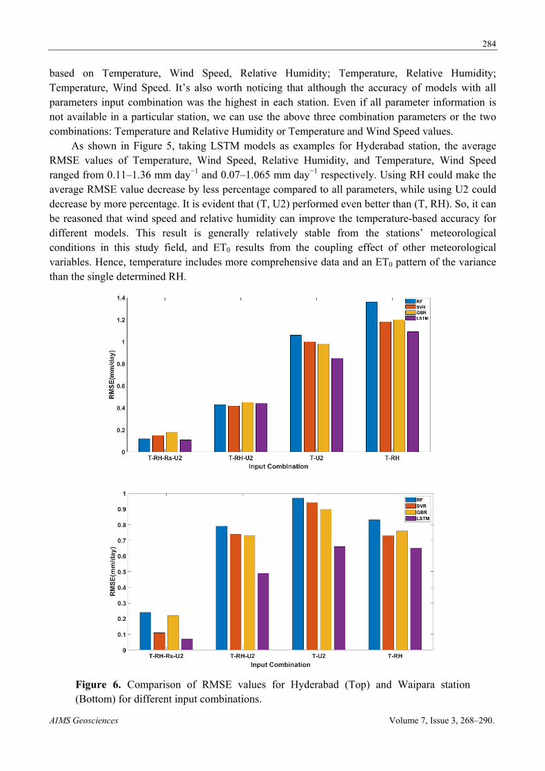
As shown in Figure 5, taking LSTM models as examples for Hyderabad station, the average RMSE values of Temperature, Wind Speed, Relative Humidity, and Temperature, Wind Speed ranged from 0.11–1.36 mm day−1 and 0.07–1.065 mm day−1 respectively. Using RH could make the average RMSE value decrease by less percentage compared to all parameters, while using U2 could decrease by more percentage. It is evident that (T, U2) performed even better than (T, RH). So, it can be reasoned that wind speed and relative humidity can improve the temperature-based accuracy for different models. This result is generally relatively stable from the stations’ meteorological conditions in this study field, and ET0 results from the coupling effect of other meteorological variables. Hence, temperature includes more comprehensive data and an ET0 pattern of the variance than the single determined RH.

Figure 6. Comparison of RMSE values for Hyderabad (Top) and Waipara station (Bottom) for different input combinations.

285


7. Discussion

This paper investigated the four ML models in estimating daily reference evapotranspiration, including LSTM, GBR, RF, and SVR with Penman-Monteith as a standard reference model with four various input combinations at semi-arid climate conditions of Hyderabad and Waipara Stations. We have reportingly found that LSTM performed the best at two stations. Three other models like SVR, GBR and RF were also used to estimate ET0. We have seen that they have also produced lower RMSE values and accurate R2 values for these stations. Various studies in literature by [30,61–64], which used ANN, LSTM, RF, SVR for ET0 estimation, reportingly found ANN, LSTM, and SVR performed best. The present study also acts as proof for the performance of these. In the present study, we have also seen that LSTM outperformed, followed by SVR and GBR. But our studies have also used different input combinations and concluded that even when two input combinations like temperature and Wind Speed are used, LSTM works well in comparison with two input combinations like Temperature and relative humidity.

From table 3, we have observed that, while some of the ML models performed well in terms of both accuracy and computational demand, which can be seen clearly in the case of LSTM and SVR. The LSTM model is appealing due to its efficiency and low test RMSE and irrespective of input combination. Notably, the multi-layer neural networks tested in this study performed better than the other machine learning models. The multi neural networks and deep learning models showed more evidence of overfitting than other mentioned machine learning models, and it is worth noticing the performance metrics for LSTM and SVR ranging R2 values to 0.99. Comparison of different machine learning and deep learning models and their performance when inputs were reduced showed the lowest performance in the case of RF and GBR models. The two input combinations, Temperature and Relative Humidity did not work well with other models, but they worked comparatively well with LSTM. So, LSTM can be used even if there are two input combinations followed by the SVR model. It has also shown that this study resembles the assessment of reference evapotranspiration found by [63] where SVR, was found to be used as an alternative ET0 estimation model to the subsistence of conventional methods. Whereas other two models RF and GBR, performed best when more inputs were used, and their performance gradually reduced when inputs combinations were brought down. [65] and [66] both reported that machine learning methods developed with regional data outperformed empirical equations. strategy showed in the current investigation can be embraced in different domains and regions as done in this paper, namely Hyderabad (India) and Waipara (New Zealand). The results obtained in this study can be compared with other empirical methods and computational models in future studies. The analysis of this presented work contributes essential guidance to use these models to estimate ET0, where partial meteorological variables and topographical data are absent and, in turn, providing ease for agriculturists, water resources management and hydrological engineers. In the future, proposed models can be applied for irrigation scheduling, evaluating the crop coefficients for crop water modelling and in estimating Actual Evapotranspiration.

To summarize, in the present study, the result of using RH with only Temperature data for assessing ET0 was also the same as previous studies done by [63] , where As a parameter for calculating RH, with limited inputs, U2 could increase modelling accuracy and be even better than RH. Hence, models based on U2 as input and LSTM model can be suggested for calculating ET0 in the light of data availability.

286


8. Conclusions

In this study comparison of four machine learning models, namely LSTM, SVR, GBR, RF, was made to know their potential in the estimation of ET0 with four different input combinations at two different stations.

The study investigated that the best performance was when all input variables were used, the study, however, finds that even three input variable combination (Temperature, Wind Speed and Relative Humidity values) or two combination input variables (Temperature and Relative Humidity, Temperature and Wind Speed) also can provide practically identical results as using all data.

The study proved that first priority can be given to model where all parameters are used as inputs, followed by three and two input combinations .

The results showed that the LSTM model could offer the most remarkable performance among four tested models regardless of station or input combination, trailed by SVR and GBR models, which could likewise accomplish moderately good performance.

Among five ML models LSTM and SVR models depend on just temperature, relative humidity, and wind speed data to achieve good performance with the fewest meteorological variables, which can be viewed as more practicality and more helpful for advancement and application. Then comes the combination of Temperature and wind speed, followed by temperature and Relative Humidity. Other models did not show remarkable results as LSTM and SVR when the above input combinations were used.

So, we concluded that even if not all parameter information is available in a particular station, we can use the above three combination parameters or the two combinations, which are temperature and wind speed or temperature and relative humidity values, to estimate reference ET0.

At spatiotemporal scales, LSTM and SVR models demonstrated extraordinary pertinence in displaying ET0 and can be strongly suggested for assessing ET0 when meteorological information is fragmented or restricted.

Acknowledgments

The Science & Engineering Research Board sponsors the research work presented in the paper, Department of Science & Technology, Government of India, Project no. YSS/2015/002111 through a start-up research grant (SRG) for Young Scientists to Dr. S. Rehana. The authors sincerely thank Professor Jayashankar Telangana State Agricultural University (PJTSAU), Rajendranagar, Hyderabad, India, for providing meteorological data. The authors would also like to thanks editor and three reviewers for their constructive comments, which has improve the paper.

Conflict of interest

The authors declare no conflict of interest.

References

1. Thornthwaite CW (1948) An Approach toward a Rational Classification of Climate. Geogr Rev 38: 55–94.

287


2. Shiri J (2019) Evaluation of a neuro‐fuzzy technique in estimating pan evaporation values in low‐altitude locations. Meteoro Appl 26: 204–212.

3. Singh SK, Marcy N (2017) Comparison of Simple and Complex Hydrological Models for Predicting Catchment Discharge Under Climate Change. AIMS Geosci 3: 467–497.

4. Verhoef W, Bach H (2003) Remote sensing data assimilation using coupled radiative transfer models. Phys Chem Earth Parts ABC 28: 3–13.

5. Biazar SM, Dinpashoh Y, Singh VP (2019) Sensitivity analysis of the reference crop evapotranspiration in a humid region. Environ Sci Pollut Res 26: 32517–32544.

6. Allen RG (1998) Food and Agriculture Organization of the United Nations, Eds., Crop evapotranspiration: guidelines for computing crop water requirements. Rome: Food and Agriculture Organization of the United Nations.

7. Landeras G, Ortiz-Barredo A, López JJ (2008) Comparison of artificial neural network models and empirical and semi-empirical equations for daily reference evapotranspiration estimation in the Basque Country (Northern Spain). Agric Water Manag 95: 553–565.

8. Tabari H, Grismer ME, Trajkovic S (2013) Comparative analysis of 31 reference evapotranspiration methods under humid conditions. Irrig Sci 31: 107–117.

9. Penman HL (1948) Natural Evaporation from Open Water, Bare Soil and Grass. Proc R Soc Lond Ser Math Phys Sci 193: 120–145. Available from: http://www.jstor.org/stable/98151.

10. Almorox J, Quej VH, Martí P (2015) Global performance ranking of temperature-based approaches for evapotranspiration estimation considering Köppen climate classes. J Hydrol 528: 514–522.

11. Ventura F, Spano D, Duce P, et al. (1999) An evaluation of common evapotranspiration equations. Irrig Sci 18: 163–170.

12. McKenney MS, Rosenberg NJ (1993) Sensitivity of some potential evapotranspiration estimation methods to climate change. Agric For Meteorol 64: 81–110.

13. Priestley CHB, Taylor RJ (1972) On the Assessment of Surface Heat Flux and Evaporation Using Large-Scale Parameters. Mon Weather Rev 100: 81–92.

14. Hargreaves GH, Samani ZA (1985) Reference Crop Evapotranspiration from Temperature. Appl Eng Agric 1: 96–99.

15. Traore S, Guven A (2012) Regional-Specific Numerical Models of Evapotranspiration Using Gene-Expression Programming Interface in Sahel. Water Resour Manag 26: 4367–4380.

16. Citakoglu H, Cobaner M, Haktanir T, et al. (2014) Estimation of Monthly Mean Reference Evapotranspiration in Turkey. Water Resour Manag 28: 99–113.

17. Kisi O, Sanikhani H (2015) Prediction of long-term monthly precipitation using several soft computing methods without climatic data. Int J Climatol 35: 4139–4150.

18. Yassin MA (2016) Artificial neural networks versus gene expression programming for estimating reference evapotranspiration in arid climate. Agric Water Manag 163: 110–124.

19. Patil AP, Deka PC (2016) An extreme learning machine approach for modeling evapotranspiration using extrinsic inputs. Comput Electron Agric 121: 385–392.

20. Antonopoulos VZ, Antonopoulos AV (2017) Daily reference evapotranspiration estimates by artificial neural networks technique and empirical equations using limited input climate variables. Comput Electron Agric 132: 86–96.

21. Granata F (2019) Evapotranspiration evaluation models based on machine learning algorithms—A comparative study. Agric Water Manag 217: 303–315..

288


22. Nourani V, Elkiran G, Abdullahi J (2019) Multi-station artificial intelligence based ensemble modeling of reference evapotranspiration using pan evaporation measurements. J Hydrol 577: 123958.

23. Dou X, Yang Y (2018) Evapotranspiration estimation using four different machine learning approaches in different terrestrial ecosystems. Comput Electron Agric 148: 95–106.

24. Ferreira LB, da Cunha FF, de Oliveira RA, et al. (2019) Estimation of reference evapotranspiration in Brazil with limited meteorological data using ANN and SVM—A new approach. J Hydrol 572: 556–570.

25. Kisi O (2007) Evapotranspiration modelling from climatic data using a neural computing technique. Hydrol Process 21: 1925–1934.

26. Wei ZW, Yoshimura K, Wang L, et al. (2017) Revisiting the contribution of transpiration to global terrestrial evapotranspiration: Revisiting Global ET Partitioning. Geophys Res Lett 44: 2792–2801.

27. Chauhan S, Shrivastava RK (2009) Performance Evaluation of Reference Evapotranspiration Estimation Using Climate Based Methods and Artificial Neural Networks. Water Resour Manag 23: 825–837.

28. Cobaner M (2011) Evapotranspiration estimation by two different neuro-fuzzy inference systems. J Hydrol 398: 292–302.

29. Suryavanshi S, Pandey A, Chaube UC, et al. (2014) Long-term historic changes in climatic variables of Betwa Basin, India. Theor Appl limatol 117: 403–418.

30. Sonali P, Nagesh Kumar D (2016) Spatio-temporal variability of temperature and potential evapotranspiration over India. J Water Clim Change 7: 810–822.

31. Saggi MK, Jain S (2019) Reference evapotranspiration estimation and modeling of the Punjab Northern India using deep learning. Comput Electron Agric 156: 387–398.

32. Pal M, Deswal S (2009) M5 model tree based modelling of reference evapotranspiration. Hydrol Process 23: 1437–1443.

33. Huang C, Davis LS, Townshend JRG (2002) An assessment of support vector machines for land cover classification. Int J Remote Sens 23: 725–749.

34. Manikumari N, Vinodhini G, Murugappan A (2020) Modelling of Reference Evapotransipration using Climatic Parameters for Irrigation Scheduling using Machine learning. ISH J Hydraul Eng 1–10.

35. Zhang JF, Zhu Y, Zhang XP, et al. (2018) Developing a Long Short-Term Memory (LSTM) based model for predicting water table depth in agricultural areas. J Hydrol 561: 918–929.

36. Kakkad V, Patel M, Shah M (2019) Biometric authentication and image encryption for image security in cloud framework. Multiscale Multidiscip Model Exp Des 2: 233–248.

37. Talaviya T, Shah D, Patel N, et al. (2020) Implementation of artificial intelligence in agriculture for optimisation of irrigation and application of pesticides and herbicides. Artif Intell Agric 4: 58–73.

38. McMillan HK, Clark MP, Bowden WB, et al. (2011) Hydrological field data from a modeller’s perspective: Part 1. Diagnostic tests for model structure. Hydrol Process 25: 511–522.

39. Singh SK, Ibbitt R, Srinivasan MS, et al. (2017) Inter-comparison of experimental catchment data and hydrological modelling. J Hydrol 550: 1–11.

40. Breiman L (2001) Random Forests. Mach Learn 45: 5–32.

289


41. Friedman JH (2001) Greedy function approximation: A gradient boosting machine. Ann Stat 29: 1189–1232.

42. Liu Y, Hejazi M, Li H, et al. (2018) A hydrological emulator for global applications—HE v1.0.0. Geosci Model Dev 11: 1077–1092.

43. Mao H, Meng J, Ji F, et al. (2019) Comparison of Machine Learning Regression Algorithms for Cotton Leaf Area Index Retrieval Using Sentinel-2 Spectral Bands. Appl Sci 9: 1459.

44. Antunes A, Andrade-Campos A, Sardinha-Lourenço A, et al. (2018) Short-term water demand forecasting using machine learning techniques. J Hydroinf 20: 1343–1366.

45. Najafzadeh M, Oliveto G (2020) Riprap incipient motion for overtopping flows with machine learning models. J Hydroinf 22: 749–767.

46. Pradhan B (2013) A comparative study on the predictive ability of the decision tree, support vector machine and neuro-fuzzy models in landslide susceptibility mapping using GIS. Comput Geosci 51: 350–365.

47. Rutkowski L, Jaworski M, Pietruczuk L, et al. (2014) The CART decision tree for mining data streams. Inf Sci 266: 1–15.

48. Tsangaratos P, Ilia I (2016) Landslide susceptibility mapping using a modified decision tree classifier in the Xanthi Perfection, Greece. Landslide 13: 305–320.

49. Balk B, Elder K (2000) Combining binary decision tree and geostatistical methods to estimate snow distribution in a mountain watershed. Water Resour Res 36: 13–26.

50. Tehrany MS, Pradhan B, Jebur MN (2013) Spatial prediction of flood susceptible areas using rule based decision tree (DT) and a novel ensemble bivariate and multivariate statistical models in GIS. J Hydrol 504: 69–79.

51. Vapnik V, Golowich SE, Smola A (1996) Support vector method for function approximation, regression estimation and signal processing. In Proceedings of the 9th International Conference on Neural Information Processing Systems, Denver, Colorado, 281–287.

52. Wang W, Xu D, Chau K, et al. (2013) Improved annual rainfall-runoff forecasting using PSO-SVM model based on EEMD. J Hydroinf 15: 1377–1390.

53. Salcedo‐Sanz S, Rojo‐Álvarez JL, Martínez‐Ramón M, et al. (2014) Support vector machines in engineering: an overview. WIREs Data Min Knowl Discov 4: 234–267.

54. Ma G, Chao Z, Zhang Y, et al. (2018) The application of support vector machine in geotechnical engineering. IOP Conf Ser Earth Environ Sci 189: 022055.

55. Sadrfaridpour E, Razzaghi T, Safro I, et al. (2019) Engineering fast multilevel support vector machines. Mach Learn 108: 1879–1917.

56. Ehteram M, Singh VP, Ferdowsi A, et al. (2019) An improved model based on the support vector machine and cuckoo algorithm for simulating reference evapotranspiration. Plos One 14: e0217499.

57. KIŞI O, ÇIMEN M (2009) Evapotranspiration modelling using support vector machines/ Modélisation de l’évapotranspiration à l’aide de “support vector machines”. Hydrol Sci J 54: 918–928.

58. Tikhamarine Y, Malik A, Pandey K, et al. (2020) Monthly evapotranspiration estimation using optimal climatic parameters: efficacy of hybrid support vector regression integrated with whale optimization algorithm. Environ Monit Assess 192: 696.

59. Dibike Y, Velickov S, Solomatine D, et al. (2001) Model Induction With Support Vector Machines: Introduction and Applications. J Comput Civ Eng 15.

290


60. Lima AR, Cannon AJ, Hsieh WW (2012) Downscaling temperature and precipitation using support vector regression with evolutionary strategy. In The 2012 International Joint Conference on Neural Networks (IJCNN), 1–8.

61. Carter C, Liang S (2019) Evaluation of ten machine learning methods for estimating terrestrial evapotranspiration from remote sensing. Int J Appl Earth Obs Geoinformation 78: 86–92.

62. Chen ZJ, Zhu ZC, Jiang H, et al. (2020) Estimating daily reference evapotranspiration based on limited meteorological data using deep learning and classical machine learning methods. J Hydrol 591: 125286.

63. Raza A, Shoaib M, Faiz MA, et al. (2020) Comparative Assessment of Reference Evapotranspiration Estimation Using Conventional Method and Machine Learning Algorithms in Four Climatic Regions. Pure Appl Geophys 177: 4479–4508.

64. Wu T, Zhang W, Jiao X, et al. (2020) Comparison of five Boosting-based models for estimating daily reference evapotranspiration with limited meteorological variables. Plos One 15: e0235324.

65. Feng Y, Peng Y, Cui N, et al. (2017) Modeling reference evapotranspiration using extreme learning machine and generalized regression neural network only with temperature data. Comput Electron Agric 136: 71–78.

66. Shiri J (2017) Evaluation of FAO56-PM, empirical, semi-empirical and gene expression programming approaches for estimating daily reference evapotranspiration in hyper-arid regions of Iran. Agric Water Manag 188: 101–114.

© 2021 the Author(s), licensee AIMS Press. This is an open access article distributed under the terms of the Creative Commons Attribution License (http://creativecommons.org/licenses/by/4.0)

Documents

Estimation of reference evapotranspiration using machine