Operational Actual Wetland Evapotranspiration Estimation

Remote Sens. 2015, 7, 3613-3632; doi:10.3390/rs70403613

remote sensing ISSN 2072-4292

www.mdpi.com/journal/remotesensing

Article

Operational Actual Wetland Evapotranspiration Estimation for South Florida Using MODIS Imagery

Cristobal N. Ceron 1, Assefa M. Melesse 1,*, René Price 1,2, Shimelis B. Dessu 1

and Hari P. Kandel 1

1 Department of Earth and Environment, Florida International University, Miami, FL 33199, USA;

E-Mails: [email protected] (C.N.C.); [email protected] (R.P.); [email protected] (S.B.D.);

[email protected] (H.P.K.) 2 Southeast Environmental Research Center, Florida International University, Miami,

FL 33199, USA

* Author to whom correspondence should be addressed; E-Mail: [email protected];

Tel.: +1-305-348-6518.

Academic Editors: Alisa L. Gallant and Prasad S. Thenkabail

Received: 13 October 2014 / Accepted: 18 March 2015 / Published: 26 March 2015

Abstract: Evapotranspiration is a reliable indicator of wetland health. Wetlands are an

important and valuable ecosystem on the South Florida landscape. Accurate wetland

Actual Evapotranspiration (AET) data can be used to evaluate the performance of South

Florida’s Everglades restoration programs. However, reliable AET measurements rely on

scattered point measurements restricting applications over a larger area. The objective of

this study was to validate the ability of the Simplified Surface Energy Balance (SSEB)

approach and the Simple Method (also called the Abtew Method) to provide large area

AET estimates for wetland recovery efforts. The study used Moderate Resolution Imaging

Spectroradiometer (MODIS) sensor spectral data and South Florida Water Management

District (SFWMD) solar radiation data to derive weekly AET values for South Florida. The

SSEB-Simple Method approach provided acceptable results with good agreement with

observed values during the critical dry season period, when cloud cover was low

(rave (n = 59) = 0.700, pave < 0.0005), but requires further refinement to be viable for yearly

estimates because of poor performance during wet season months, mainly because of cloud

contamination. The approach can be useful for short-term wetland recovery assessment

projects that occur during the dry season and/or long term projects that compare site AET

rates from dry season to dry season.

OPEN ACCESS

Remote Sens. 2015, 7 3614

Keywords: everglades; evapotranspiration; MODIS; simple model; SSEB;

surface temperature

1. Introduction

Wetlands provide a wide range of services and benefits to a region. They provide erosion protection

to coastlines and sediment control for large areas [1]. Wetlands provide extensive habitats for a wide

range of wildlife, including nursery habitats for numerous fish and shellfish species and breeding,

nursing, and migratory habitat for large numbers of water birds [2]. Wetlands are habitats for many

species of reptiles, amphibians, some mammals, and a myriad of insect and plant species [1–3].

Wetlands act as a giant filter cleaning both natural and man-made waste, help recharge aquifers, and

provide drinking water for communities [2,3]. In addition, wetlands can be ideal sites for recreational

activities such as camping, fishing, and hunting and for educational and scientific study [4].

Loss of wetlands is a worldwide problem, and the United States has experienced major losses in

recent history. It is estimated that during the late part of the 20th century, the United States was losing

wetlands at the rate of 60,000 acres per year [5]. Fortunately, concerted conservation and remediation

efforts have helped slow the loss of wetland environments. South Florida is dominated by three major

ecosystems: natural, agricultural, and urban. The eastern edge of South Florida is covered mostly by

urban sprawl in close proximity to extensive natural areas to the west and south. These natural areas

include Everglades National Park, Big Cypress National Preserve, Biscayne National Park, and many

smaller wild wetland areas. Agricultural lands are scattered across the South Florida landscape,

particularly in the Everglades Agricultural Area near and around the southern edge of Lake

Okeechobee. Understanding the interactions between the three closely linked ecological systems can

help improve existing design approaches of wetland restoration and conservation plans that balance the

needs of people with environmental sustainability.

The unique and diverse characteristics of wetlands have indirectly contributed to their destruction in

many areas. Over the years, wetlands have been drained or had their water sources diverted to control

flooding in developed (or soon to be developed) areas [1,4]. Wetlands also have been drained to take advantage of their nutrient-rich soils for agricultural production or grazing of livestock [4,6]. Wetlands

that are not directly developed continue to suffer from the effects of urban and agricultural

development. Runoff from agricultural and urban areas can pollute wetlands, affecting the natural

chemistry of these areas [1]. Many of these problems currently affect one of the largest wetland environments in the world: South Florida’s Everglades National Park.

Evapotranspiration as an Indicator of Wetland Recovery

With many restoration efforts now underway, evaluations are necessary to assess the success of the

restoration methods being used. Water has a direct impact on the ecosystem dynamics of wetlands, and

hydrologic variables such as evapotranspiration, flood duration, flow velocity, and flow variability can

be used to gauge wetland health [7–9]. Of these hydrological variables, evapotranspiration (ET) proves

a reliable indicator of hydrological recovery [10]. ET is the combined measurement of water being lost


to the atmosphere as a result of evaporation from open water sources and transpiration from plants. In

general, ET is the principal method of water loss in South Florida wetlands. For example, the

Everglade receives a yearly average rainfall of around 1270 mm and loses an estimated 1020 mm

annually to ET [11]. The difference between rainfall and ET can be used to measure the workings of

healthy wetland ecosystems.

Various methods exist for estimating ET. Traditional means, such as the pan, Bowen ratio, eddy

correlation, and aerodynamic techniques, estimate ET at point locations. These methods are costly, time consuming, and require elaborate and sensitive measurement equipment [12]. A root-zone soil

water balance approach based on a water budget is also a technique used to estimate ET as a residual

variable. Quantifying each component of the soil water balance is less appealing in terms of time,

labor, and money requirements. Relatively simpler point methods use lysimeter instrumentation [13].

Although the traditional methods estimate ET on a point basis, recent methods have found success

using remotely sensed imagery for estimates at various spatial scales [14,15]. In contrast to point

measurements, remote sensing has the capacity to acquire spectral signatures instantaneously for large

areas of the watershed across multiple electromagnetic (EM) wavebands and spatial scales. Data in

multiple EM wavebands allow for the extraction of land cover, vegetation cover, emissivity, albedo,

surface temperature, energy flux information, and data at regional scales allow for greater spatial

coverage than possible with in-situ methods.

Various researchers have used remote sensing tools to estimate wetland evapotranspiration and

energy fluxes in various regions of the world [16–25]. A healthy wetland area will be fully or partially

inundated for most of the year. The water will provide the necessary conditions for wetland flora and

fauna to grow and thrive. The combination of surface water and healthy plant populations will cause

high rates of both evaporation and transpiration (high ET). Conversely, an unhealthy and dry wetland

area lacks the necessary flooding to maintain the growth of native flora. The lack of above-surface

water and healthy plant population result in low evaporation and transpiration rates (low ET). Hence,

measuring the ET rates of a restored wetland and comparing them with the ET rates of healthy

wetlands can provide a measure of how well the treated wetland is recovering. Furthermore, studying

ET rates over prolonged periods of time can provide information on the speed and efficiency of the

restoration techniques applied at a given site. Although ET is recognized as an important measure of

wetland health, identifying the best-suited technique for measurement of ET in the South Florida

region is a credible research question. We tested one such approach.

Rainfall measurements are made at numerous locations across South Florida, but ET stations are

rare. Satellite measurements allow for wide spatial coverage between land-based stations, and provide

visible access to relatively inaccessible areas such as the Everglades. The objective of this study was to

assess and validate a model that will provide weekly Actual Evapotranspiration (AET) estimates for

the South Florida region using the “Simple Method” technique in combination with the Simplified

Surface Energy Balance Method (SSEB), which we describe in the methods section. The study

produced AET estimates and maps for the South Florida region, with a focus on wetland areas in and

around Everglades National Park and Big Cypress National Preserve. These products can be used

operationally to assess the progress of wetland restoration. Hence, results of this research will facilitate

future restoration assessment studies by providing a simple and accessible method of calculating

ET values.


2. Study Area, Data Set and Methods

2.1. Description of the Study Area

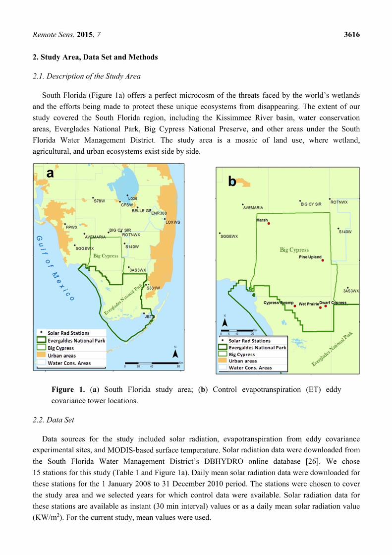
South Florida (Figure 1a) offers a perfect microcosm of the threats faced by the world’s wetlands

and the efforts being made to protect these unique ecosystems from disappearing. The extent of our

study covered the South Florida region, including the Kissimmee River basin, water conservation

areas, Everglades National Park, Big Cypress National Preserve, and other areas under the South

Florida Water Management District. The study area is a mosaic of land use, where wetland,

agricultural, and urban ecosystems exist side by side.

Figure 1. (a) South Florida study area; (b) Control evapotranspiration (ET) eddy

covariance tower locations.

2.2. Data Set

Data sources for the study included solar radiation, evapotranspiration from eddy covariance experimental sites, and MODIS-based surface temperature. Solar radiation data were downloaded from

the South Florida Water Management District’s DBHYDRO online database [26]. We chose

15 stations for this study (Table 1 and Figure 1a). Daily mean solar radiation data were downloaded for

these stations for the 1 January 2008 to 31 December 2010 period. The stations were chosen to cover

the study area and we selected years for which control data were available. Solar radiation data for

these stations are available as instant (30 min interval) values or as a daily mean solar radiation value

(KW/m2). For the current study, mean values were used.


Table 1. List and location of solar radiation stations.

Station Basin Latitude Longitude County Description

3AS3WX Conservation

area 3A 25°51′6.2″ 80°45′58.5″ Miami-Dade

Water Conservation Area 3 (WCA3)

weather station, tree islands.

Ave Maria Faka Union 26°18′6.09″ 81°25′52.9″ Collier Town of Ave Maria weather station

BELLE GL S-2_6_7 26°39′24.6″ 80°37′48.1″ Palm Beach Belle Glade weather station

BIG CY SIR Feeder Canal 26°19′17.3″ 81°4′4.24″ Hendry Big Cypress at Seminole

Indian Reservation

CFSW S-4 26º44′6.23″ 80°53′43.2″ Hendry Clewinston field station

weather station

ENR308 STA-1W 26°37′21.2″ 80°26′20.2″ Palm Beach Weather station near interior

levee in cell 3

FPWX Estero Bay 26°25′57.3″ 81°43′24.3″ Lee Flint Pen Strand weather station

JBTS C-111 Coastal 25°13′28.4″ 80°32′24.2″ Miami-Dade

Joe Bay, approx. 9.5 km from

Gilbert’s Res. Overseas Hwy boat

ramp, key Largo

L006 Lake

Okeechobee 26°49′21.2″ 80°46′58.2″ Palm Beach Lake Okeechobee tower South (#6)

LOXWS Conservation

area 1 26°29′56.3″ 80°13′20.2″ Palm Beach

Loxahatchee weather station at

CA1-8C and L-40

ROTNWX STA-5/6 26°19′56.8″ 80°52′53.1″ Broward Rotenberger tract weather station

S140W Conservation

Area 3A 26°10′16.7″ 80°49′33.6″ Broward

S140 weather station on levee L28

near Alligator Alley

S331W L-31NS 25°36′37.5″ 80°30′34.6″ Miami-Dade S-331 weather station on L-31N

S78W East

Caloosahatchee 26°47′23.2″ 81°18′10.3″ Glades

S-78 weather station on

Caloosahatchee River at Ortona

SGGEWX Faka Union 26°8′43.3″ 81°34′32.3″ Collier Southern Golden Gate Estates

weather station

Surface temperature data from the Moderate Resolution Imaging Spectroradiometer (MODIS)

onboard NASA’s Terra satellite were used in this study. The MODIS instrument has 36 spectral bands

to take images of the Earth at resolutions of 250, 500, and 1000 meters, providing information on

cloud/aerosol properties, ocean phytoplankton densities, and surface and cloud temperature, among

other atmospheric, land, and ocean surface phenomena. MODIS provided the necessary temporal

(weekly) dimensions needed to estimate weekly evapotranspiration rates across the expansive South

Florida Region. The 1000 m spatial resolution of the thermal band of MODIS is also sufficient to

capture the spatial variability of evapotranspiration.

We downloaded the MOD11A2 MODIS Land Surface Temperature (LST) and Emissivity eight-day

product from the Land Processes Distribution Active Archive Center [27]. The MODIS sensor collects

raw digital signals to calculate reflectance and Earth-exiting radiance [28]. The MOD11A2 product consists of 12 layers, including clear day/night average LSTs and emissivity values as well as several

quality assurance layers. LST is calculated using MODIS radiance data (MOD021KM) in combination

with MODIS geolocation data (MOD03), atmospheric temperature and water profile data

(MOD07_L2), cloud mask data (MOD35_L2), and land-cover (MOD12Q1) and snow cover data

(MOD10_L2) [29]. The MOD11A2 product is composited from eight days of daily 1-km LST


products (MOD11A1) to create average (across the eight days) clear-sky LSTs. To be classified as

“clear sky” an image or pixel must pass the “clear sky” validation process detailed by Ackerman [30].

MODIS products are projected onto a sinusoidal grid of “tiles” composed of 36 columns and 18 rows.

The study area is located in tile (10, 6), where the first number corresponds to the column and the

second to the row of the grid. Images from 1 January 2008 to 31 December 2010, were downloaded

from the U.S. Geological Survey’s (USGS) EarthExplorer ordering interface [31]. There are 46

eight-day intervals per year, resulting in a total of 138 time intervals across the three years we studied.

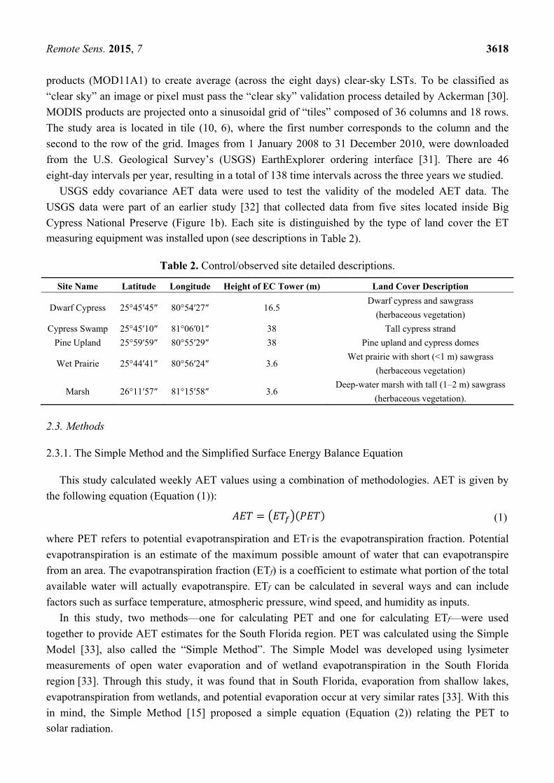
USGS eddy covariance AET data were used to test the validity of the modeled AET data. The

USGS data were part of an earlier study [32] that collected data from five sites located inside Big

Cypress National Preserve (Figure 1b). Each site is distinguished by the type of land cover the ET measuring equipment was installed upon (see descriptions in Table 2).

Table 2. Control/observed site detailed descriptions.

Site Name Latitude Longitude Height of EC Tower (m) Land Cover Description

Dwarf Cypress 25°45′45″ 80°54′27″ 16.5 Dwarf cypress and sawgrass

(herbaceous vegetation)

Cypress Swamp 25°45′10″ 81°06′01″ 38 Tall cypress strand

Pine Upland 25°59′59″ 80°55′29″ 38 Pine upland and cypress domes

Wet Prairie 25°44′41″ 80°56′24″ 3.6 Wet prairie with short (<1 m) sawgrass

(herbaceous vegetation)

Marsh 26°11′57″ 81°15′58″ 3.6 Deep-water marsh with tall (1–2 m) sawgrass

(herbaceous vegetation).

2.3. Methods

2.3.1. The Simple Method and the Simplified Surface Energy Balance Equation

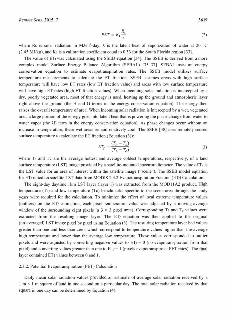
This study calculated weekly AET values using a combination of methodologies. AET is given by

the following equation (Equation (1)):

(1)

where PET refers to potential evapotranspiration and ETf is the evapotranspiration fraction. Potential

evapotranspiration is an estimate of the maximum possible amount of water that can evapotranspire

from an area. The evapotranspiration fraction (ETf) is a coefficient to estimate what portion of the total

available water will actually evapotranspire. ETf can be calculated in several ways and can include

factors such as surface temperature, atmospheric pressure, wind speed, and humidity as inputs.

In this study, two methods—one for calculating PET and one for calculating ETf—were used

together to provide AET estimates for the South Florida region. PET was calculated using the Simple

Model [33], also called the “Simple Method”. The Simple Model was developed using lysimeter

measurements of open water evaporation and of wetland evapotranspiration in the South Florida

region [33]. Through this study, it was found that in South Florida, evaporation from shallow lakes,

evapotranspiration from wetlands, and potential evaporation occur at very similar rates [33]. With this

in mind, the Simple Method [15] proposed a simple equation (Equation (2)) relating the PET to solar radiation.


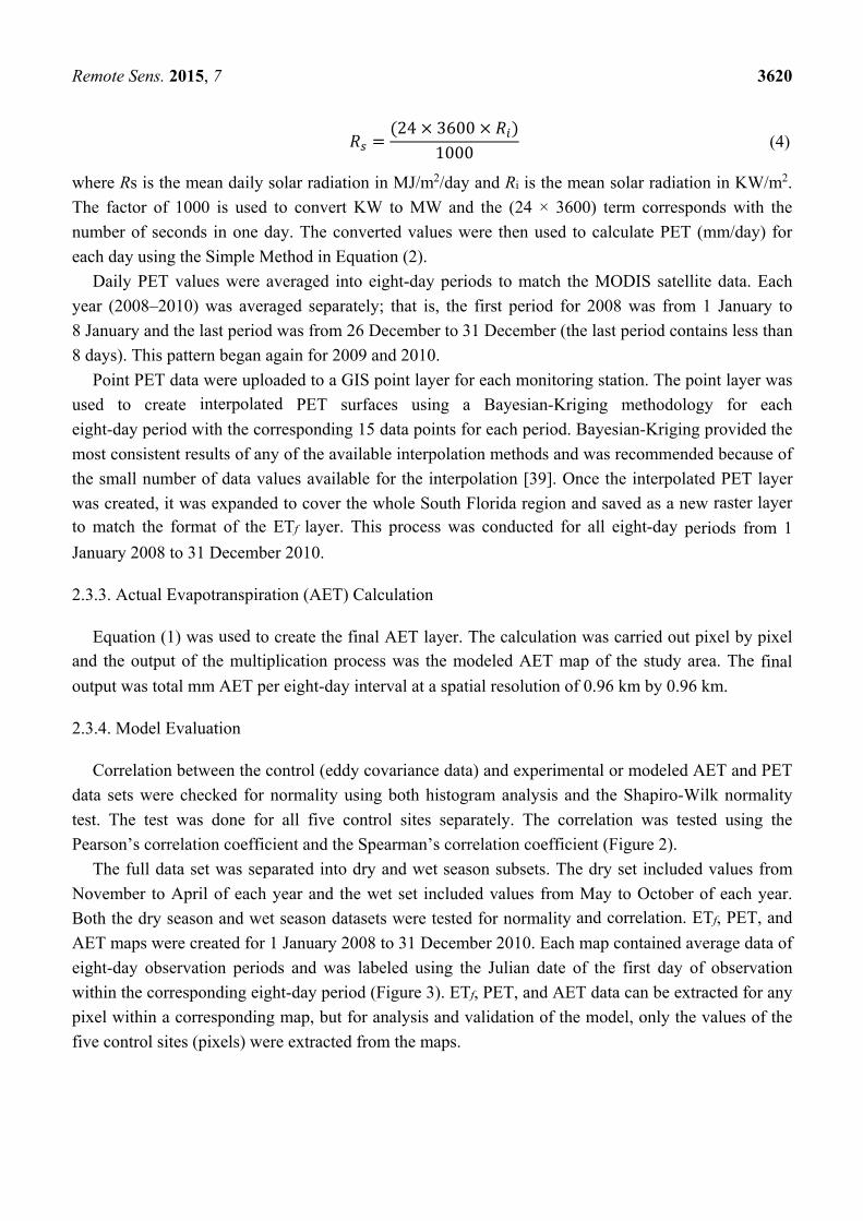
(2)

where Rs is solar radiation in MJ/m2-day, λ is the latent heat of vaporization of water at 20 °C

(2.45 MJ/kg), and K1 is a calibration coefficient equal to 0.53 for the South Florida region [33].

The value of ETf was calculated using the SSEB equation [34]. The SSEB is derived from a more

complex model Surface Energy Balance Algorithm (SEBAL) [35–37]. SEBAL uses an energy

conservation equation to estimate evapotranspiration rates. The SSEB model utilizes surface

temperature measurements to calculate the ET fraction. SSEB assumes areas with high surface

temperature will have low ET rates (low ET fraction value) and areas with low surface temperature

will have high ET rates (high ET fraction values). When incoming solar radiation is intercepted by a

dry, poorly vegetated area, most of that energy is used, heating up the ground and atmospheric layer

right above the ground (the H and G terms in the energy conservation equation). The energy then

raises the overall temperature of area. When incoming solar radiation is intercepted by a wet, vegetated

area, a large portion of the energy goes into latent heat that is powering the phase change from water to

water vapor (the λE term in the energy conservation equation). As phase changes occur without an

increase in temperature, these wet areas remain relatively cool. The SSEB [38] uses remotely sensed surface temperature to calculate the ET fraction (Equation (3)):

(3)

where Th and Tc are the average hottest and average coldest temperatures, respectively, of a land

surface temperature (LST) image provided by a satellite-mounted spectroradiometer. The value of Tx is

the LST value for an area of interest within the satellite image (“scene”). The SSEB model equation for ETf relied on satellite LST data from MODIS.2.3.2 Evapotranspiration Fraction (ETf) Calculation.

The eight-day daytime 1km LST layer (layer 1) was extracted from the MOD11A2 product. High

temperature (Th) and low temperature (Tc) benchmarks specific to the scene area through the study

years were required for the calculation. To minimize the effect of local extreme temperature values

(outliers) on the ETf estimation, each pixel temperature value was adjusted by a moving-average

window of the surrounding eight pixels (a 3 × 3 pixel area). Corresponding Th and Tc values were

extracted from the resulting image layer. The ETf equation was then applied to the original (un-averaged) LST image pixel by pixel using Equation (3). The resulting temperature layer had values

greater than one and less than zero, which correspond to temperature values higher than the average high temperature and lower than the average low temperature. These values corresponded to outlier

pixels and were adjusted by converting negative values to ETf = 0 (no evapotranspiration from that pixel) and converting values greater than one to ETf = 1 (pixels evapotranspire at PET rates). The final

layer contained ETf values between 0 and 1.

2.3.2. Potential Evapotranspiration (PET) Calculation

Daily mean solar radiation values provided an estimate of average solar radiation received by a

1 m × 1 m square of land in one second on a particular day. The total solar radiation received by that square in one day can be determined by Equation (4):


24 36001000

(4)

where Rs is the mean daily solar radiation in MJ/m2/day and Ri is the mean solar radiation in KW/m2.

The factor of 1000 is used to convert KW to MW and the (24 × 3600) term corresponds with the

number of seconds in one day. The converted values were then used to calculate PET (mm/day) for

each day using the Simple Method in Equation (2).

Daily PET values were averaged into eight-day periods to match the MODIS satellite data. Each

year (2008–2010) was averaged separately; that is, the first period for 2008 was from 1 January to

8 January and the last period was from 26 December to 31 December (the last period contains less than

8 days). This pattern began again for 2009 and 2010.

Point PET data were uploaded to a GIS point layer for each monitoring station. The point layer was

used to create interpolated PET surfaces using a Bayesian-Kriging methodology for each

eight-day period with the corresponding 15 data points for each period. Bayesian-Kriging provided the

most consistent results of any of the available interpolation methods and was recommended because of

the small number of data values available for the interpolation [39]. Once the interpolated PET layer

was created, it was expanded to cover the whole South Florida region and saved as a new raster layer to match the format of the ETf layer. This process was conducted for all eight-day periods from 1

January 2008 to 31 December 2010.

2.3.3. Actual Evapotranspiration (AET) Calculation

Equation (1) was used to create the final AET layer. The calculation was carried out pixel by pixel and the output of the multiplication process was the modeled AET map of the study area. The final

output was total mm AET per eight-day interval at a spatial resolution of 0.96 km by 0.96 km.

2.3.4. Model Evaluation

Correlation between the control (eddy covariance data) and experimental or modeled AET and PET

data sets were checked for normality using both histogram analysis and the Shapiro-Wilk normality

test. The test was done for all five control sites separately. The correlation was tested using the

Pearson’s correlation coefficient and the Spearman’s correlation coefficient (Figure 2).

The full data set was separated into dry and wet season subsets. The dry set included values from

November to April of each year and the wet set included values from May to October of each year.

Both the dry season and wet season datasets were tested for normality and correlation. ETf, PET, and

AET maps were created for 1 January 2008 to 31 December 2010. Each map contained average data of

eight-day observation periods and was labeled using the Julian date of the first day of observation

within the corresponding eight-day period (Figure 3). ETf, PET, and AET data can be extracted for any

pixel within a corresponding map, but for analysis and validation of the model, only the values of the

five control sites (pixels) were extracted from the maps.


Figure 2. Correlation test results between control site ET and modeled ET. Error bars

represent confidence level (p-value).

Figure 3. Potential evapotranspiration (PET), the evapotranspiration fraction (ETf), and

actual evapotranspiration (AET) maps for observation period 2008025. This period

includes data from 25 January to 1 February of 2008.


3. Results and Discussion

3.1. Correlation between Modeled and Observed AET

The modeled AET was in close agreement with observed eddy covariance data, with a correlation

coefficient of rave (n = 59) = 0.700 and pave < 0.0005 for the dry season, when wetland management is

critical because of high temperatures and the absence of rainfall (Figure 2). For the wet season, the MODIS images were covered with clouds and the LST data were not accurate enough to give results as

good as that of the dry season.

3.2. Modeled AET Temporal Variation

The model showed varying degrees of success depending on the time of year. There was a clear

distinction between certain parts of each year. MODIS temperature data for hotter, wetter months

(August and September) had a higher incidence of missing data (due to cloud cover) and pixels of

lower temperature values than images acquired during cooler, dryer months (December, January).

Hence, the data were stratified by a “Dry” period and a “Wet” period to see how each distinct season

affected the overall trends observed in the complete dataset.

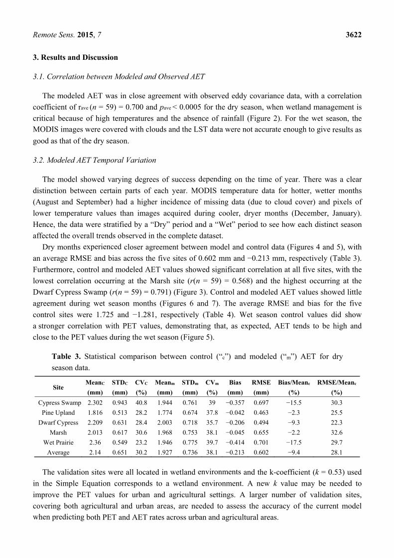
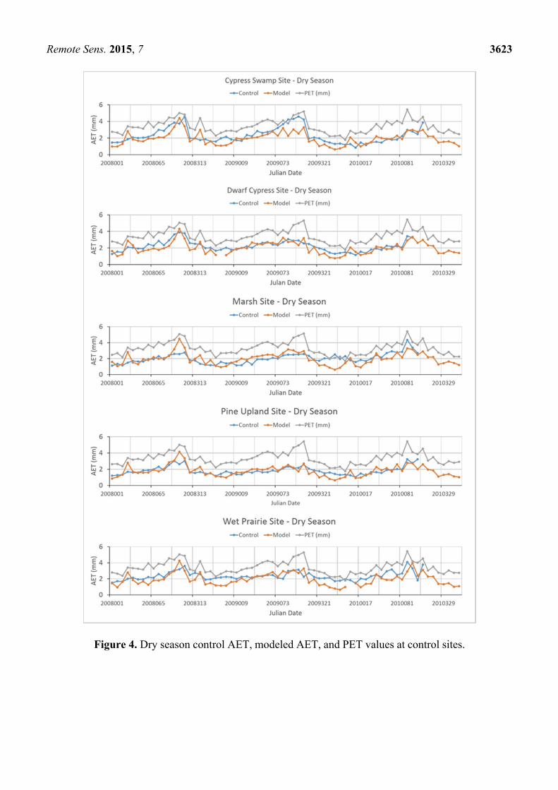
Dry months experienced closer agreement between model and control data (Figures 4 and 5), with

an average RMSE and bias across the five sites of 0.602 mm and −0.213 mm, respectively (Table 3).

Furthermore, control and modeled AET values showed significant correlation at all five sites, with the

lowest correlation occurring at the Marsh site (r(n = 59) = 0.568) and the highest occurring at the

Dwarf Cypress Swamp (r(n = 59) = 0.791) (Figure 3). Control and modeled AET values showed little

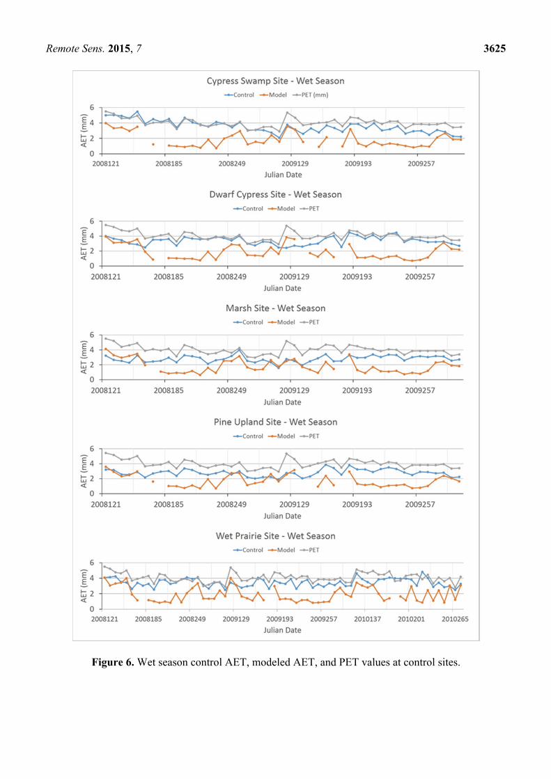
agreement during wet season months (Figures 6 and 7). The average RMSE and bias for the five

control sites were 1.725 and −1.281, respectively (Table 4). Wet season control values did show

a stronger correlation with PET values, demonstrating that, as expected, AET tends to be high and

close to the PET values during the wet season (Figure 5).

Table 3. Statistical comparison between control (“c”) and modeled (“m”) AET for dry

season data.

Site MeanC

(mm)

STDC

(mm)

CVC

(%)

Meanm

(mm)

STDm

(mm)

CVm

(%)

Bias

(mm)

RMSE

(mm)

Bias/Meanc

(%)

RMSE/Meanc

(%)

Cypress Swamp 2.302 0.943 40.8 1.944 0.761 39 −0.357 0.697 −15.5 30.3

Pine Upland 1.816 0.513 28.2 1.774 0.674 37.8 −0.042 0.463 −2.3 25.5

Dwarf Cypress 2.209 0.631 28.4 2.003 0.718 35.7 −0.206 0.494 −9.3 22.3

Marsh 2.013 0.617 30.6 1.968 0.753 38.1 −0.045 0.655 −2.2 32.6

Wet Prairie 2.36 0.549 23.2 1.946 0.775 39.7 −0.414 0.701 −17.5 29.7

Average 2.14 0.651 30.2 1.927 0.736 38.1 −0.213 0.602 −9.4 28.1

The validation sites were all located in wetland environments and the k-coefficient (k = 0.53) used

in the Simple Equation corresponds to a wetland environment. A new k value may be needed to

improve the PET values for urban and agricultural settings. A larger number of validation sites,

covering both agricultural and urban areas, are needed to assess the accuracy of the current model when predicting both PET and AET rates across urban and agricultural areas.


Figure 4. Dry season control AET, modeled AET, and PET values at control sites.


Figure 5. Dry season comparisons between control and modeled AET data.


Figure 6. Wet season control AET, modeled AET, and PET values at control sites.


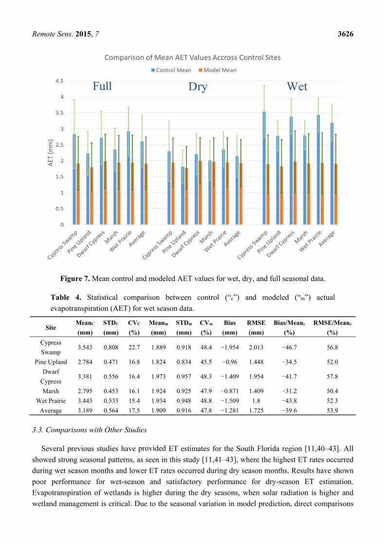
Figure 7. Mean control and modeled AET values for wet, dry, and full seasonal data.

Table 4. Statistical comparison between control (“c”) and modeled (“m”) actual

evapotranspiration (AET) for wet season data.

Site MeanC

(mm)

STDC

(mm)

CVC

(%)

Meanm

(mm)

STDm

(mm)

CVm

(%)

Bias

(mm)

RMSE

(mm)

Bias/Meanc

(%)

RMSE/Meanc

(%)

Cypress

Swamp 3.543 0.808 22.7 1.889 0.918 48.4 −1.954 2.013 −46.7 56.8

Pine Upland 2.784 0.471 16.8 1.824 0.834 45.5 −0.96 1.448 −34.5 52.0

Dwarf

Cypress 3.381 0.556 16.4 1.973 0.957 48.3 −1.409 1.954 −41.7 57.8

Marsh 2.795 0.453 16.1 1.924 0.925 47.9 −0.871 1.409 −31.2 50.4

Wet Prairie 3.443 0.533 15.4 1.934 0.948 48.8 −1.509 1.8 −43.8 52.3

Average 3.189 0.564 17.5 1.909 0.916 47.8 −1.281 1.725 −39.6 53.9

3.3. Comparisons with Other Studies

Several previous studies have provided ET estimates for the South Florida region [11,40–43]. All

showed strong seasonal patterns, as seen in this study [11,41–43], where the highest ET rates occurred

during wet season months and lower ET rates occurred during dry season months. Results have shown

poor performance for wet-season and satisfactory performance for dry-season ET estimation.

Evapotranspiration of wetlands is higher during the dry seasons, when solar radiation is higher and

wetland management is critical. Due to the seasonal variation in model prediction, direct comparisons


between seasonal ET rates from this model and others were made. Abtew [33] used lysimeters to

calculate ET of a marsh site from 1993 to 1994. Average ET of dry season months (November to

April) was 3.16 mm/day in 1993 (January estimate not included) and 2.74 mm/day in 1994. The lowest

dry season ET of the study period corresponded to January of 1994 (1.9 mm/day) and the highest ET

corresponded to April of 1993 (4.8 mm/day). Douglas [41] conducted a broader study using the

Priestly-Taylor and Penman-Monteith methods to calculate ET for a wide range of sites across Florida

including marsh sites inside Everglades National Park and a few pine forest sites in Northern Florida.

The marsh sites showed an average ET of 3.0 mm/day and the pine forest sites had an average ET of

2.05 mm/day [38]. Estimates from lysimeter sites (sawgrass and cattail) carried out from 1996 to 1999

gave dry season ET average estimates ranging from 1.42 mm/day (January cattail) to 4.9 mm/day

(April sawgrass) [44]. Dry season ET estimates ranging from about 1.5 mm/day to about 4.5 mm/day

are seen in the majority of ET studies of wetland regions across Florida [11,41–43].

The ET estimates calculated in this study fell within the range discussed in the aforementioned

studies (Table 5). For example, the marsh site had a dry season average of 1.97 mm/day over the

observation period, which was lower than the average seen at similar sites in the Abtew [33] and

Douglas [41] studies. Similarly, the Pine Upland site had an average dry season of 1.77 mm/day,

which again was lower than the ET estimates of previous studies. The control values provided by

Shoemaker [32], 2.01 mm/day for the Marsh site and 1.82 mm/day for the Pine Upland site, showed

that the low dry season ET estimates were not necessarily due to poor model performance, but that the

dry season ET rates estimated during the study period were lower than those of previous study periods.

The average experimental dry season ET across all five control sites was 1.92 mm/day, which fell

within the range of ET values observed in previous studies [11,33,41]. The average control dry season

AET across all five sites was 2.14 mm/day. These averages show that the model did tend to

underestimate the AET values for all five sites.

Table 5. Comparison of evapotranspiration (ET) values from different studies.

Source Dry Season Wet Season Site

SSEB−Simple Method 1.92 mm/day 1.91 mm/day Average of 5 sites

Mao et al. [44] 1.42 mm/day to 4.9 mm/day Lysimeter (sawgrass

& cattail) German [11], Douglas et al. [41],

Abtew [42], Bidlake et al. [43] 1.5 mm/day 4.5 mm/day Wetland regions

Abtew [33] 3.16 mm/day in 1993 2.74 mm/day in 1994

Lysimeter marsh site from 1993 to 1994

Allen [45] has stated that AET estimates through remote sensing methods can expect errors (defined

as one standard deviation away from the true mean) between 10% and 30%. The metric in this study

that provided the most similar definition of error as defined by Allen was RMSE/Meanc (mean of the

control values), which also gave an estimate of how far away the experimental values fell from the true

values (in this case taken to be the control values). The average RMSE/Meanc of the five control sites

was 28.1%, meaning that, on average, the experimental values were about 30% away from the control

values. In a similar study, Jiang [46] used daily LST data to provide daily AET estimates in the South

Florida region. His results showed a range for RMSE/Meanc from 23.1% to 45% across 11 sites, with


an average of 30.8%, which again is similar to the RMSE/Meanc observed across the five sites used in

this study for dry season months. In general, the Simple/SSEB method provided AET estimates in line

with previous studies using relatively simple techniques that did not require the technical expertise, large equipment and maintenance costs, or time needed by other methods [41,42,47,48].

3.4. Limitations and Suggested Improvements

The calculation of AET estimates carried out in this study faced common challenges identified in

similar wetland AET estimation studies. First and foremost, prolonged periods of cloud cover during

wet season months had a deleterious effect on the LST data provided by the MODIS sensor. This led to

the underestimation of ETf and, consequently, AET estimates. Jiang [46] also faced the problem of

cloudy images and applied a model where missing pixels were approximated by using neighboring pixels and pixels from previous observations. This can work, but not when a large portion of the

observation area is cloud covered for the better part of eight days (from this study). The ability to

acquire useful LST data under cloudy conditions would definitely have improved the AET estimates

provided by this study and remains a major challenge for any methodology that relies on remotely

sensed data to provide useful AET estimates for South Florida or other cloud-prone regions.

Missing and underestimated LST data from MODIS was the main source of error for the final AET

values for the wet season. The eight-day composite temperature images were created by averaging the “clear sky” pixels from eight single-day temperature images. Defining a “clear sky” pixel is a rather

complex endeavor, as detailed in Ackerman [30], but a clear sky pixel is free from most, if not all,

cloud contamination. To have a missing pixel in the eight-day composite image, the majority (or all) of

the single-day images must have that pixel missing, as well (i.e., cloud covered). But, there is a chance

that a clear sky pixel exists within one of the eight single-day images. The single-day LST data can

overcome poor eight-day LST images where temperature values can be used to calculate the ETf for

the pixel of interest. For now, the more appropriate solution for this problem is the acquisition of better

temperature data, which may be available from other satellite based sensors with thermal bands, such

as ASTER and Landsat [49]. Improvements to the ETf estimation procedure can also help improve the accuracy of final AET

estimates. This is currently being done in other studies that incorporate more complex techniques of

calculating Th and Tc [38,50]. The approaches being tested may increase the accuracy of the final AET

estimates, but they do so at the expense of simplicity. The use of other remote sensing platforms that

can provide higher resolution data and/or complement the data provided by MODIS would also improve the accuracy of AET estimates. Lastly, ground-based temperature measurements may help fill

in data gaps found in the MODIS LST images.

4. Conclusions and Recommendations

Long-term evapotranspiration patterns can be used to detect the health of wetlands. The combined

Simple Method and SSEB ET estimation model tested for use in restoration assessment of the

Everglades of South Florida provided acceptable results under dry season conditions. On one hand,

AET estimates provided by the model had good agreement with control eddy covariance based ET

values during dry season months. For these dry months, the model proved to be both applicable and


useful and provided AET values that may inform wetland recovery assessments. ET in wetlands is

highest in these months due to high solar radiation, and wetland management and monitoring also are

critical during this period. On the other hand, AET was underestimated for wet season months. The

main source of error for wet month AET estimates came from poor LST data from the MODIS sensor

due to prolonged periods of cloud cover.

The Simple Method approach provided acceptable results with good agreement with observed values

during the critical dry season period, when cloud cover was low (rave(n = 59) = 0.7, pave < 0.0005), but

requires further refinement to be viable for yearly estimates because of poor performance during wet season months, mainly because of cloud contamination. The model showed promise as a quick and

simple monitoring tool for wetland recovery on an operational basis. Such products have been lacking to

help evaluate the restoration of the Everglades. The simplicity of the model, requiring only temperature

and solar radiation data, can produce results comparable to more complex methods when the input data

are of good quality. Furthermore, this study demonstrated the model’s ability to successfully cover areas

as large as the South Florida region. Weekly accurate estimates seem feasible for dry season months,

when ET is highly dynamic spatiotemporally, and its estimation is very important. Several aspects of the Simple Model/SSEB approach tested in this study can benefit from further

refinement. First and foremost, better methods of gathering LST data are needed to replace data gaps

during the cloudy wet season. Second, a larger network of solar radiation monitoring stations would

help create more accurate PET maps for the South Florida region. Finally, ETf calculations may benefit from the introduction of new parameters (not just temperature) to increase the accuracy of final

AET estimates.

Acknowledgments

The authors acknowledge the South Florida Water Management District and the USGS and NASA

for the data used in this study. Melesse’s time was supported by the NASA-funded WaterSCAPES project. Participation by RM Price was supported by the Florida Coastal Everglades Long-Term

Ecological Research program under National Science Foundation Grant No. DEB-1237517.

Author Contributions

Melesse and Price provided technical advice and reviewed several iterations of the paper for content

and format accuracy. Dessu and Kandel provided guidance and resources during the data analysis

portion of the study.

Conflict of Interest

The authors declare no conflicts of interest in this work.

References

1. Maltby, E.; Barker, T. Section II: Wetlands in the natural environment, how do wetlands work? In

The Wetlands Handbook; Maltby, E., Barker, T., Eds.; Wiley: Oxford, UK, 2009; Volume 2,

pp. 115–326.


2. Abers, J.S.; Pavri, S.; Aber, S.A. Part I and Part II. In Wetland Environments: A Global

Perspective; Wiley-Blackwell: Chichester, UK, 2012; pp. 1–132.

3. LePage, B.A. Wetlands: A multidisciplinary perspective. In Wetlands: Integrating

Multidisciplinary Concepts, 1st ed.; Springer: New York, NY, USA, 2011; pp. 3–25.

4. Abtew, W.; Melesse, A.M. Chapter 6: Evaporation and evapotranspiration estimation methods.

In Evaporation and Evapotranspiration: Measurements and Estimations; Abtew, W.,

Melesse, A.M., Eds.; Springer: Dordrecht, The Netherlands, 2013; pp. 63–91.

5. Davis, D. Threats to Wetlands. Available online: http://permanent.access.gpo.gov/gpo701/

threats.pdf (accessed on 18 September 2013).

6. Mitsch, W.G.; Gosselink, J.G. The Wetland Environment. In Wetlands, 4th ed.; John Wiley &

Sons: New York, NY, USA, 2000; pp. 107–258.

7. Gurnell, A.M.; Hupp, C.R.; Gregory, S.V. Linking hydrology and ecology. Hydrol. Process.

2000, 14, 2813–2815.

8. Price, J.S.; Waddington, J.M. Advances in Canadian wetland hydrology and biogeochemistry.

Hydrol. Process. 2000, 14, 1579–1589.

9. Janssen, R.; Goosen, H.; Verhoeven, M.L.; Verhoeven, J.T.A.; Omtzigt, A.Q.A.; Maltby, E.

Decision support for integrated wetland management. Environ. Model. Softw. 2005, 20, 215–229.

10. Oberg, J.W.; Melesse, A.M. Wetland evapotranspiration dynamics vs. ecohydrological

restoration: An energy balance and remote sensing approach. J. Am. Water Resourc. Assoc. 2005,

42, 565–582.

11. German, E.R. Regional Evaluation of Evapotranspiration in the Everglades; Water-Resources

Investigations Report 00-4217; US Geological Survey: Tallahassee, FL, USA, 2000; p. 48.

12. Monteith, J.L.; Unsworth, M.H. Principles of Environmental Physics, 2nd ed.;

Butterworth-Heinemann: Woburn, MA, USA, 1990.

13. Brooks, K.N.; Ffolliott, P.F.; Gregersen, H.M.; DeBano, H.F. Hydrology and the Management of

Watersheds, 2nd ed.; Iowa State University Press: Ames, IA, USA, 1997.

14. Tateishi, R.; Ahn, C.H. Mapping evapotranspiration and water balance for global land surfaces.

ISPRS J. Photogramm. Remote Sens. 1996, 51, 209–215.

15. Mauser, W.; Schadlich, S. Modeling the spatial distribution of evapotranspiration on different

scales using remote sensing data. J. Hydrol. 1998, 212–213, 250–267.

16. Melesse, A.; Nangia, V.; Wang, X.; McClain, M. Wetland restoration response analysis using

MODIS and groundwater data. Sensors 2007, 7, 1916–1933.

17. Glenn, E.P.; Mexicano, L.; Garcia-Hernandez, J.; Naglerc, P.L.; Gomez-Sapiensa, M.M.;

Tanga, D.; Lomelid, M.A.; Ramirez-Hernandezd, J.; Zamora-Arroyoe, F. Evapotranspiration and

water balance of an anthropogenic coastal desert wetland: Responses to fire, inflows and

salinities. Ecol. Eng. 2013, 59, 176–184.

18. Melesse, A.M.; Oberg, J.; Beeri, O.; Nangia, V.; Baumgartner, D. Spatiotemporal dynamics of

evapotranspiration and vegetation at the glacial ridge prairie restoration. Hydrol. Process. 2006,

20, 1451–1464.

19. Zhao, X.; Liu, Y. Lake fluctuation effectively regulates wetland evapotranspiration: A case study

of the largest freshwater lake in China. Water 2014, 6, 2482–2500.


20. Li, Z.; Liu, X.; Ma, T.; Kejia, D.; Zhou, Q.; Yao, B.; Niua, T. Retrieval of the surface

evapotranspiration patterns in the alpine grassland-wetland ecosystem applying SEBAL model in

the source region of the Yellow River, China. Ecol. Eng. 2013, 270, 64–75.

21. Venturini, V.; Bisht, G.; Islam, S.; Jiang, L. Comparison of evaporative fractions estimated from

AVHRR and MODIS sensors over South Florida. Remote Sens. Environ. 2004, 93, 77–86.

22. Jiang, L.; Islam, S. Estimation of surface evaporation map over southern great plains using remote

sensing data. Water Resour. Res. 2001, 37, 329–340.

23. Jiang, L.; Islam, S.; Jutla, A.; Senarath, S.; Ramsey, B.H.; Eltahir, E. An intercomparison of regional

latent heat flux estimation using remote sensing data. Int. J. Remote Sens. 2009, 24, 2221–2236.

24. Lagomasino, D.; Price, R.M.; Whitman, D.; Melesse, A.M.; Oberbauer, S. Spatial and temporal

variability in spectral-based evapotranspiration measured from Landsat 5TM across two mangrove

ecotones. Agric. For. Meteorol. 2014, doi:10.1016/j.agrformet.2014.11.017.

25. Senay, G.B.; Verdin, J.P.; Lietzow, R.; Melesse, A.M. Global daily reference evapotranspiration

modeling and validation. J. Am. Water Resour. Assoc. 2008, 44, 969–979.

26. DBHYDRO Available online: http://xportal.sfwmd.gov/dbhydroplsql/show_dbkey_info.main_menu

(accessed on 15 March 2014).

27. LP DAAC. Available online: https://lpdaac.usgs.gov/data_access (accessed on 10 February 2014).

28. Toller, GN; Isaacman, A. MODIS Level 1B Product User’s Guide; NASA/Goddard Space Flight

Center: Greenbelt, MD, USA, 2012; p. 56.

29. Wan, Z. Collection-5 MODIS Land Surface Temperature Products User’s Guide; University of

California: Santa Barbara, CA, USA, 2006.

30. Ackerman, S.; Frey, R.; Strabala, K.; Liu, Y.; Gumley, L.; Baum, B.; Menzel, P. Discriminating

Clear-Sky from Cloud with MODIS Algorithm Theoretical Basis Document (MOD35);

Cooperative Institute for Meteorological Satellite Studies, University of Wisconsin-Madison:

Madison, WI, USA, 2010; p. 20.

31. Earth Explorer Available online: http://earthexplorer.usgs.gov (accessed on 02 February 2014).

32. Shoemaker, W.B.; Lopez, C.D.; Duever, M.J. Evapotranspiration over Spatially Extensive Plant

Communities in the Big Cypress National Preserve, Southern Florida, 2007-2010; U.S.

Geological Survey SIR 2011-5212; U.S. Geological Survey, Reston, VA, USA, 2011; p. 46.

33. Abtew, W. Evapotranspiration measurements and modeling for three wetland systems in South

Florida. J. Am. Water Resour. Assoc. 1996, 32, 465–473.

34. Senay, G.B.; Budde, M.; Verdin, J.P.; Melesse, A.M. A coupled remote sensing and simplified

surface energy balance approach to estimate actual evapotranspiration from irrigated fields.

Sensors 2007, 7, 979–1000.

35. Bastiaanssen, W.G.M.; Menenti, M.; Feddes, R.A.; Holtslag, A.A.M. A remote sensing surface

energy balance algorithm for land (SEBAL) 1. Formulation. J. Hydrol. 1998, 212–213, 198–212.

36. Bastiaanssen, W.G.M.; Pelgrum, H.; Wang, J.; Ma, Y.; Moreno, J.F.; Roerink, G.J.; van der Wal, T.

A remote sensing Surface Energy Balance Algorithm for Land (SEBAL) 2. Validation. J. Hydrol.

1998, 212–213, 213–229.

37. Bastiaanssen, W.G.M.; Noordman, E.J.M.; Pelgrum, H.; Davids, G.; Thoreson, B.P.; Allen, R.G.

SEBAL model with remotely sensed data to improve water-resources management under actual

field conditions. J. Irrig. Drain. Eng. 2005, 131, 85–93.


38. Senay, G.B.; Bohms, S.; Singh, R.K.; Gowda, P.H.; Velpuri, N.M.; Alemu, H.;Verdin, J.P.

Operational evapotranspiration mapping using remote sensing and weather datasets: A new

parameterization for the SSEB approach. J. Am. Water Resour. Assoc. 2013, 49, 577–591.

39. Pilz, J.; Spöck, G. Why do we need and how should we implement Bayesian Kriging methods.

Stoch. Environ. Res. Risk Assess. 2007, 22, 621–632.

40. Abtew, W.; Obeysekera, J.; Irizarry-Ortiz, M.; Lyons, D.; Reardon, A. Evapotranspiration

estimation for South Florida. In Proceedings of World Water and Environmental Resources

Congress 2003, Philadelphia, PA, USA, 22–26 June 2003; doi:10.1061/40685(2003)235.

41. Douglas, E.M.; Jacobs, J.M.; Sumner, D.M.; Ray, R.L. A comparison of models for estimating

potential evapotranspiration for Florida land cover types. J. Hydrol. 2009, 373, 366–376.

42. Abtew, W. Comparison of Bowen Ratio Measurements and Model Estimations. In

Evapotranspiration in the Everglades; South Florida Water Management District: West Palm

Beach, FL, USA, 2004; pp. 2–13.

Bidlake, W.R.; Woodham, W.M.; Lopez, M.A. Evapotranspiration from Areas of Native

Vegetation in West-Central Florida; Water-Supply Paper 2430; U.S. Geological Survey:

Washington, DC, USA, 1996.

43. Mao, L.M.; Bergman, M.J.; Tai, C.C. Evapotranspiration measurement and estimation of three

wetland environments in the Upper St. Johns River Basin, Florida. J. Am. Water Resour. Assoc.

2002, 38, 1271–1285.

44. Allen, R.G.; Pereira, L.S.; Howell, T.A.; Jensen, M.E. Evapotranspiration information reporting:

I. Factors governing measurement accuracy. Agric. Water Manag. 2011, 98, 899–920.

45. Jiang, L.; Islam, S.; Guo, W.; Jutla, A.S.; Senarath, S.U.S.; Ramsay, B.H.; Eltahir, E.

A satellite-based daily actual evapotranspiration estimation algorithm over South Florida. Glob.

Planet. Chang. 2009, 67, 62–77.

46. Enku, T.; van der Tol, C.; Gieske, A.; Rientjes, T. Chapter 8: Evapotranspiration modeling using

remote sensing and empirical models in the Fogera Floodplain. In Nile River Basin: Hydrology,

Climate and Water Use; Melesse A.M., Ed.; Springer: Dordrecht, The Netherlands, 2011;

pp. 163–178.

47. Courault, D.; Seguin, B.; Olioso, A. Review on estimation of evapotranpiration from remote

sensing data: From empirical to numerical modeling approaches. Irrig. Drain. Syst. 2005,

19, 223–249.

48. Allen, R.G.; Tasumi, M.; Morse, A.; Trezza, R.A. Landsat-based energy balance and

evapotranspiration model in Western US water rights regulation and planning. Irrig. Drain. Syst.

2005, 19, 251–268.

49. Savoca, M.E.; Senay, G.B.; Maupin, M.A.; Kenny, J.F.; Perry, C.A. Actual Evapotranspiration

Modeling Using Operational Simplified Surface Energy Balance (SSEBop) Approach; U.S.

Geological Survey: Reston, VA, USA, 2013; p. 14.

© 2015 by the authors; licensee MDPI, Basel, Switzerland. This article is an open access article

distributed under the terms and conditions of the Creative Commons Attribution license

(http://creativecommons.org/licenses/by/4.0/).

Documents

Operational Actual Wetland Evapotranspiration Estimation