A Parametric Model for Potential Evapotranspiration Estimation

Chapter 8

A Parametric Model for PotentialEvapotranspiration Estimation Based on a SimplifiedFormulation of the Penman-Monteith Equation

Aristoteles Tegos, Andreas Efstratiadis andDemetris Koutsoyiannis

Additional information is available at the end of the chapter

http://dx.doi.org/10.5772/52927

1. Introduction

The estimation of evapotranspiration is a typical task in several disciplines of geosciencesand engineering, including hydrology, meteorology, climatology, ecology and agriculturalengineering. According to the specific area of interest, we distinguish between three differ‐ent aspects of evapotranspiration, i.e. actual, potential and reference crop. In particular, theactual evapotranspiration refers to the quantity of water that is actually removed from a sur‐face due to the combined processes of evaporation and transpiration. At the global scale, it isestimated that about 60% of precipitation reaching the Earth’s terrain returns to the atmos‐phere by means of water losses due to evapotranspiration [1]. Obviously this percentage isnot constant but exhibits significant variability both in space and time. In particular, in semi-arid basins the annual percentage of evapotranspiration losses may be 70-80% of precipita‐tion, while in cold hydroclimates this percentage is lower that 30%.

The actual evapotranspiration is one of the most difficult processes to measure in the field,except for experimental, small-scale areas, for which lysimeter observations can be assumedrepresentative. For the spatial scale of practical applications (e.g., river basin), there is agrowing interest on remote sensing technologies, which attempt to estimate actual evapo‐transpiration at regional scales, by combining ground measurements with satellite-deriveddata [2]. Otherwise, the only reliable method is based on the calculation of the water balanceof the basin. Apparently, this approach is valid only when actual evapotranspiration is thesingle unknown component of the water balance. In addition, it can be implemented onlyfor large time scales (annual and over-annual), for which storage regulation effects can be

© 2013 Tegos et al.; licensee InTech. This is an open access article distributed under the terms of the CreativeCommons Attribution License (http://creativecommons.org/licenses/by/3.0), which permits unrestricted use,distribution, and reproduction in any medium, provided the original work is properly cited.

neglected. Alternatively, the spatiotemporal representation of the water balance can be eval‐uated through hydrological models. The latter simulate the main hydrological mechanismsof the river basin, using areal rainfall and potential evapotranspiration as input data. In or‐der to obtain the actual evapotranspiration, which is output of the model, it is therefore es‐sential to estimate the potential evapotranspiration across the basin.

Potential, as well as and crop reference evapotranspiration, are two key concepts, for whichdifferent definitions have been proposed, often leading to confusing interpretations [3]. Theterm “potential evapotranspiration”, introduced by Thornthwaite [4], generally refers to themaximum amount of water that could evaporate and transpire from a large and uniformlyvegetated landscape, without restrictions other than the atmospheric demand [5, 6]. On theother hand, the reference crop evapotranspiration (or reference evapotranspiration) is strict‐ly defined as the evapotranspiration rate from a reference surface, not short of water, of ahypothetical grass crop with a height of 0.12 m, a fixed surface resistance of 70 s/m and analbedo of 0.23. This description closely resembles a surface of green, well-watered grass ofuniform height, actively growing and completely shading the ground [7].

Potential and reference evapotranspiration can be theoretically retrieved on the basis ofmass transfer and energy balance approaches. In this respect, a wide number of methodsand models have been developed, of different levels of complexity. Lu et al. [6] report thatthere exist over 50 of such methods, which can be distinguished according to their mathe‐matical framework and data requirements. The most integrated approaches are the analyti‐cal (also called combination) ones, which combine energy drivers, i.e. solar radiation andtemperature, with atmospheric drivers, i.e. vapour pressure deficit and surface wind speed,towards a physically-based representation of the phenomenon [8]. In particular, Penman [9]developed the classical method named after him, which combines the energy balance andaerodynamic processes to predict the evaporation through open water, bare soil and grass.Later, Monteith [10] expanded the Penman equation to also account for the role of vegeta‐tion in controlling transpiration, particularly through the opening and closing of stomata.

The subsequently referred to as the Penman-Monteith method is by far the most recognizedamong all evapotranspiration models, as reported in numerous investigations worldwide.For instance, this approach provided the optimal estimates on the daily and monthly scalesand was the most consistent across all locations [11]. It was also indicated that the Penman-Monteith method exhibited excellent performance in both arid and humid climates [12] andwas the most accurate in estimating the water needs of turfgrass [13]. Its suitability was con‐firmed even when relative humidity and wind velocity data are missing [14].

The Penman-Monteith method requires complex calculations and it is data demanding. Inthis respect, a number of radically simplified methods have been proposed that require few‐er meteorological variables. The latter can be divided into two categories: radiation-basedapproaches, which account for both the variability of solar radiation and temperature [15,16, 17, 18], and elementary empirical methods that use as single meteorological input tem‐perature [4, 19, 20]. A comprehensive review of them is provided in [21] and [22]. Yet, thepredictive capacity of most of these models remains questionable, since they are based onempirical assumptions that do not ensure consistency with the physics of the natural phe‐

Evapotranspiration - An Overview144

nomenon. Moreover, their applicability is usually restricted to specific geographical loca‐tions and climatic regimes, because their parameters are derived from experimentsemployed at the local scale.

Except for temperature, long records of input time series for the Penman-Monteith methodare rarely available, especially in older meteorological stations. Thus, a typical problem isthe estimation of evapotranspiration, in case of missing meteorological data. The Food andAgriculture Organization (FAO) emphatically suggests employing the Penman-Monteithmethod even under limited data availability. In this context, it provides a number of proce‐dures for dealing with missing information, while it discourages the use of empirical ap‐proaches [7]. Yet, most of the proposed procedures still require meteorological data that arebarely accessible, or require arbitrary assumptions with regard to the climatic regime of thestudy area.

Here we propose an alternative parametric approach, which is founded on a simplified par‐simonious expression of the Penman-Monteith formula. The method can be assigned to ra‐diation-based approaches, yet its key difference is the use of free variables (i.e. parameters)instead of constants, which are fitted to local climatic conditions. The method is parsimoni‐ous both in terms of meteorological data requirements (temperature) and with regard to thenumber of parameters (one to three).

For the identification of parameters, it is essential to have reference time series of satisfacto‐ry accuracy, preferably estimated through the Penman-Monteith method. Under this prem‐ise, the model parameters can be obtained through calibration, thus by minimizing thedepartures between the modelled evaporation data and the reference data. This task was ap‐plied in 37 meteorological stations that are maintained by the National Meteorological Serv‐ice of Greece. As will be shown, the proposed method is clearly superior to commonly-usedempirical approaches. Moreover, by mapping the parameter values over the entire Greekterritory, using typical interpolation tools, we provide a flexible framework for the directand reliable estimation of evapotranspiration anywhere in Greece.

The article is organized as follows: In section 2, we review the Penman-Monteith methodand its simplifications, which estimate evapotranspiration on the basis of temperature andradiation data. In section 3 we present the new parametric model, which compromises therequirements for parsimony and consistency. In section 4, we calibrate the model at thepoint scale, using historical meteorological data, and evaluate it against other empirical ap‐proaches. In addition, we investigate the geographical distribution of its parameters overGreece. Finally, in section 5 we summarize the outcomes of our research and discuss nextresearch steps.

2. The Penman-Monteith method and its simplifications

2.1. The Penman method and its physical background

Evaporation can be viewed both as energy (heat) exchange and an aerodynamic process. Ac‐cording to the energy balance approach, the net radiation at the Earth’s surface (Rn = Sn – Ln,

A Parametric Model for Potential Evapotranspiration Estimationhttp://dx.doi.org/10.5772/52927

145

where Sn and Ln are the shortwave—solar—and longwave—earth—radiation, respectively)is mainly transformed to latent heat flux, Λ, and sensible heat flux to the air, H. The evapora‐tion rate, expressed in terms of mass per unit area and time (e.g. kg/m2/d), is given by theratio E΄ := Λ / λ, where λ is the latent heat of vaporization, with typical value 2460 kJ/kg. Byignoring fluxes of lower importance, such as soil heat flux, the heat balance equation issolved for evaporation, yielding:

E΄ = (Rn – H ) / λ = Rn / λ(1 + b) (1)

where b := H / Λ is the co-called Bowen ratio. The estimation of b requires the measurementof temperature at two levels (surface and atmosphere), as well as the measurement of hu‐midity at the atmosphere. On the other hand, the estimation of the net radiation Rn is basedon a radiation balance approach to determine the components Sn and Ln. Typical input datarequired (in addition to latitude and time of the year), are solar radiation (direct and diffuse,or, in absence of them, sunshine duration data or cloud cover observations), temperatureand relative humidity. The net radiation also depends of surface properties (i.e. albedo) andtopographical characteristics, in terms of slope, aspect and shadowing. Recent studiesproved that the impacts of topography are important at all spatial scales, although they areusually neglected in calculations [23].

From the aerodynamic viewpoint, evaporation is a mass diffusion process. In this context,the rate of evaporation is related to the difference in the water vapor content of the air attwo levels above the evaporating surface and a function of the wind speed F(u) in the diffu‐sion equation. Theoretically, F(u) can be computed on the basis of elevation, wind velocity,aerodynamic resistance and temperature. Yet, for simplicity it is usually given by empiricalformulas, derived through linear regression, for a standard measurement level of 2 meters.

Penman [9] combined the energy balance with the mass transfer approaches, thus allowingthe use of temperature, humidity and wind speed measurements at a single level. His classi‐cal formula for computing evaporation from an open water surface is written as:

( )nR΄ F u DD gE

D g l D g= +

+ +(2)

where Δ is the slope of vapor pressure/temperature curve at equilibrium temperature(hPa/K), γ is a psychrometrcic coefficient, with typical value 0.67 hPa/K, and D is the vaporpressure deficit of the air (hPa), defined as the difference between the saturation vapor pres‐sure ea and the actual vapor pressure es, which are functions of temperature and relative hu‐midity. We remind that (2) estimates the evaporation rate (mass per unit area per day),which is expressed in terms of equivalent water depth by dividing by the water density ρ(1000 kg/m3). Next we will use symbols Ε΄ for evaporation rates, and E := Ε΄ / ρ for equiva‐lent depths per unit time.


Summarizing, the Penman equation requires records of solar radiation (alternatively, sun‐shine duration or cloud cover), temperature, relative humidity and wind speed, as well as anumber of parameters accounting for surface characteristics (latitude, Julian day index, albe‐do, elevation, etc.).

2.2. The Penman-Monteith method

Penman’s method was extended to cropped surfaces, by accounting for various resistancefactors, aerodynamic and surface. As mentioned in the introduction, Monteith [10] intro‐duced the concept of the so-called “bulk” surface resistance that describes the resistance ofvapor flow through the transpiring crop and evaporating soil surface [7]. This depends onmultiple factors, such as the solar radiation, the vapor pressure deficit, the temperature ofleafs, the water status of the canopy, the height of vegetation, etc. Combining the two resist‐ance components, the following generalized expression of the Penman equation is obtained,referred to as Penman–Monteith formula:

( )nR΄ F u D

΄ ΄D gE

D g l D g= +

+ +(3)

where:

1 /( )s a΄ r rg g= + (4)

In the above relationship, rs and ra are the surface and aerodynamic resistance factors, re‐spectively. For water, the surface resistance is zero, thus eq. (3) is identical to the Penmanformula. For any other type of surface, the evapotranspiration can be analytically computed,provided that the two resistance parameters are known. In practice, it is extremely difficultto obtain parameter rs on the basis of typical field data, even more so because this is time-varying. Thus, its evaluation is only possible for some specific cases.

In this context, FAO proposed the application of the Penman–Monteith method for the hy‐pothetical reference crop, thus introducing the concept of reference evapotranspiration.With standardized height for wind speed, temperature and humidity measurements at 2.0m and the crop height of 0.12 m, the aerodynamic and surface resistances become ra = 208 /u2 (where u2 is the wind velocity, in m/s) and rs = 70 s/m. The experts of FAO suggested us‐ing the Penman–Monteith method as the standard for reference evapotranspiration and ad‐vised on procedures for calculation of the various meteorological inputs and parameters [7].

2.3. Radiation-based approaches

The complexity of the Penman–Monteith method stimulated many researchers to seek foralternative, simplified expressions, based on limited and easily accessible data. Given thatthe main sources of variability in evapotranspiration are temperature and solar radiation,the two variables are introduced in a number of such models, typically referred as radiation-


147

based. We note that the classification to “radiation-based” instead of the more complete “ra‐diation-temperature-based” is made for highlighting the difference with even simplerapproaches that use temperature as single input variable.

A well-known simplification is the Priestley–Taylor formula [17], which is expressed interms of equivalent depth (mm/d):

ne

RDE aD g lr

=+

(5)

where ae is a numerical coefficient, with values from 1.26 to 1.28. Thus, in the above expres‐sion, the energy term of the Penman–Monteith equation is increased by about 30%, in orderto skip over the aerodynamic term. This assumption allows for omitting the use of wind ve‐locity and surface resistance in evapotranspiration calculations.

Despite its simplifications, the Priestley–Taylor method is still physically-based, as opposedto most of radiation-based approaches that are rather empirical. In addition, many of themuse either total solar radiation or even extraterrestrial radiation, instead of net radiation da‐ta. For instance, Jensen & Haise [15], based on evapotranspiration measurements from irri‐gated areas across the United States, proposed the following expression:

40

a aR TE

l r= (6)

This equation only uses average daily temperature, Ta, and extraterrestrial radiation, Ra. Lat‐er, McGuiness & Bordne [16] suggested a slight modification of the Jensen–Haise expres‐sion, known as McGuinness model:

( ) 568

a aR TE

lr+

= (7)

Another widely used approach is the Hargreaves model [18] that estimates the referenceevapotranspiration at the monthly scale by:

( )( )0.5 ( ) 0.0023 / 17.8 –a a max minR T T TE l= + (8)

where Ta is the average monthly temperature and Tmax – Tmin is the difference between themaximum and minimum monthly temperature (oC). This method provides satisfactory re‐sults, with typical error of 10-15% or 1.0 mm/d, and it is suggested when only temperaturedata is available [24].

Many studies proved the superiority of radiation-based approaches against temperature-based ones. For instance, Lu et al. [6] compared three models from each category across SE


United States and showed that radiation-based methods produced clearly better results,with reference to pan evaporation measurements. Oudin et al. [25] investigated the suitabili‐ty of such approaches, as input to rainfall-runoff models. In this context, they evaluated anumber of evapotranspiration methods, on the basis of precipitation and streamflow datafrom a large number of catchments in U.S., France and Australia. Within their research, theyprovided a generalized expression of the Jensen–Haise and McGuinness models, i.e.

( ) 2

1

a aR T K

KE

lr+

= (9)

where K1 (°C) is a scale parameter and K2 (°C) is a parameter related to the threshold for airtemperature, i.e. the minimum value of air temperature for which evapotranspiration is notzero. The researchers tested several values of K1 and K2 for four well-known hydrologicalmodels, and kept the combination that gave the best streamflow simulations over the entirecatchment sample. After extended analysis, they concluded that the parameters are model-specific. As general recommendation, they proposed the values K1 = 100°C and K2 = 5°C.

2.4. Temperature-based approaches

The most elementary approaches only use temperature data as input, while the radiationterm is indirectly accounted for, by means of empirical or semi-empirical expressions. Themost recognized method of this category is the Thornthwaite formula [4]:

10 16

12 30

aa dT

EI

Næ ö æ öæ öç ÷ ç ÷ç ÷

è øè øè ø= (10)

where Ta is the average monthly temperature, d is the average number of daylight hours perday for each month, N is the number of days in the month, I is the so-called annual heat in‐dex, which is estimated on the basis on monthly temperature values, and a is another pa‐rameter, which is function of I. Initially, the method was applied in USA, but later it wasalso tested in a number of regions worldwide [26]. Today, this method is not recommended,since it results in unacceptably large errors. In dry climates, evapotranspiration is underesti‐mated, while in wet climates it is significantly overestimated [27].

Another widely known temperature-based method is the Blaney & Criddle formula [19]:

( ) 0.254 32 1.8 aE p T= + (11)

where p is the mean daily percentage of annual daytime hours. The method estimates thereference crop evapotranspiration on a monthly basis, and has been widely applied inGreece for the assessment of irrigation needs. Yet, the Blaney–Criddle method is only suita‐ble for rough estimations. Especially under “extreme” climatic conditions, the method is in‐


149

accurate: in windy, dry, sunny areas, the evapotranspiration is underestimated by up to60%, while in calm, humid, clouded areas it is overestimated up to 40% [26]. For this reason,several improvements of the method have been proposed. A well-known one is the modi‐fied Blaney-Criddle formula by Doorenbos & Pruitt [28], which however require additionalmeteorological inputs, thus loosing the advantage of data parsimony.

Linacre [20] has also developed simplified formulas to estimate open water evaporation andreference evapotranspiration on the basis of temperature. For the calculation of evaporation,the Linacre formula is:

( )( )

700 0.006 1( ) / ( )00 – 15 –

80 –dz T T

ET

jT + += (12)

where z is the elevation, φ is the latitude and Td is the dew point, which is also approximate‐ly derived though air temperature. For the reference evapotranspiration, the constant 700 innumerator is replaced by 500. In Greece, the Linacre method generally seriously overesti‐mates the evapotranspiration, and it is not recommended [33]. Its major drawback is the as‐sumption of a one-to-one relationship between evaporation and radiation, which is notrealistic.

We notify that all the above approaches are only valid for monthly or daily scales, which aresufficient for most of engineering applications. For shorter time scales (e.g. hourly), the esti‐mation of reference evapotranspiration requires additional astronomical calculations as wellas finely-resolved meteorological data. Empirical formulas for such time scales are alsoavailable in the literature, e.g. in [29].

3. Development of parsimonious parametric formulas forevapotranspiration modelling

3.1. The need for a parametric model

A typical shortcoming of most of simplified approaches (i.e. empirical models that use solar ra‐diation and temperature data) for evapotranspiration modeling is their poor predictive capaci‐ty against the entire range of climatic regimes and locations. For, these models are built andvalidated in specific conditions. Thus, while they work well in the areas and over the periodsfor which they have been developed, they provide inaccurate results when they are applied toother climatic areas, without reevaluating the constants involved in the empirical formulas[30]. Hence, the key idea behind the development of a parametric model is the replacement ofsome of the constants that are used in such formulas by free parameters, which are regionally-varying. The optimal values of parameters can be obtained through calibration, i.e. by fittingmodel outputs to “reference” evapotranspiration time series. Nowadays, calibration is a ratherstraightforward task, thanks to the development of powerful global optimization techniques,such as evolutionary algorithms. The reference data can be provided either directly (e.g.


through remote sensing) or estimated by well-established methods (preferably the Penman-Monteith model). Optimization is carried out against a goodness-of-fit criterion, which aggre‐gates the departures between the simulated and reference data (e.g. coefficient of efficiency).

In this context, a parametric expression can be used as a generalized regression formula, for in‐filling and extrapolating evapotranspiration records. This is of high importance, since in manyconventional meteorological stations, the temperature records usually overlap the records ofthe rest of variables that are required by the Penman-Monteith method. The use of a parametricmodel, with parameters calibrated on the basis of reliable evapotranspiration data, is obvious‐ly preferable to empirical models, which cannot account for the whole available meteorologicalinformation, i.e. the past observations of humidity, solar radiation and wind velocity.

3.2. Ensuring parsimony and consistency

The need for parsimonious models is essential in all aspects of water engineering and man‐agement [31]. Generally, the concept of parsimony refers to both the model structure, whichshould be as simple as possible, and the input data, which should be as fewer as possibleand easily available. Yet, as indicated in the Section 2, many of the empirical models forevapotranspiration estimations, although they are data parsimonious, fail to provide realis‐tic results (see also Section 4 below), since they do not account for important aspects of thenatural phenomenon. Therefore, before building the model it is crucial to ensure that sim‐plicity will not be in contrast with consistency. This requires: (a) the choice of the most im‐portant explanatory variables in the equations, and (b) the determination of the number ofparameters, which should be identified through calibration.

3

10 000

15 000

20 000

25 000

30 000

35 000

40 000

45 000

0.0 5.0 10.0 15.0 20.0 25.0 30.0

Monthly temperature, T a (oC)

Extra

terr

estri

al ra

diat

ion,

Sa (

kJ/m

2 )

0

50

100

150

200

250

300

350M

onth

ly e

vapo

ratio

n, E

(m

m)

Sa (kJ/m^2)Ε (mm)

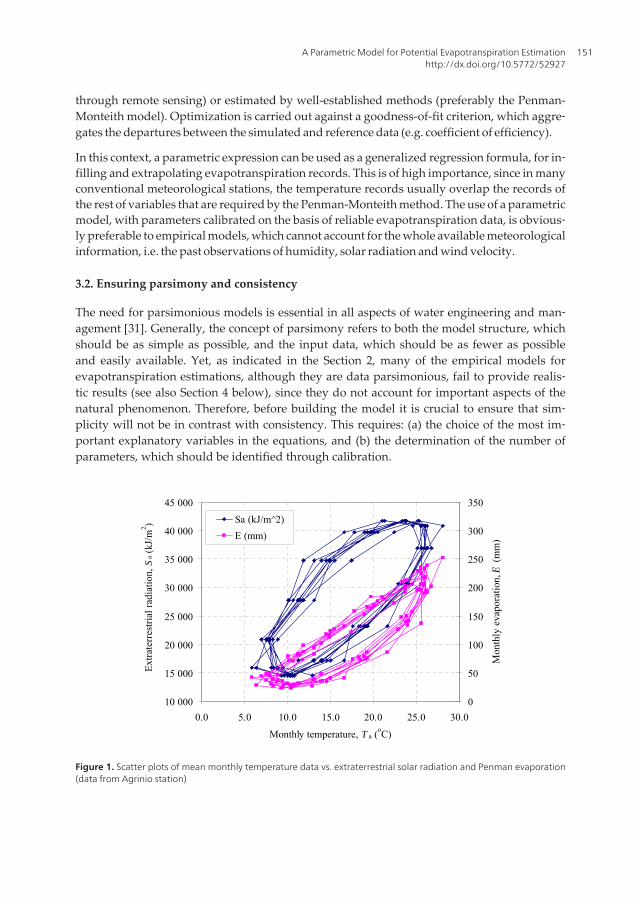
Figure 1. Scatter plots of mean monthly temperature data vs. extraterrestrial solar radiation and Penman evaporation(data from Agrinio station)


151

It is well-known that the variability of evapotranspiration is mainly explained by the var‐iability of solar radiation and temperature. Yet, instead of measured solar radiation,which is rarely available, and following the practice of most of the empirical methods,we decided to use extraterrestrial radiation, together with temperature, as explanatoryvariables in the new formula. In order to justify this option, we examined several combi‐nations of variables, using data from a number of meteorological stations in Greece. Inthe example of Figure 1 are illustrated the scatter plots of mean monthly temperature Ta,against extraterrestrial solar radiation Sa, and against monthly evaporation E, which is es‐timated through the Penman method. The data are from the Agrinio station, WesternGreece, and cover a ten-year period (1979-1988). The graphical representation of E vs. Ta

and Sa vs. Ta exhibit characteristic loop shapes, which clearly indicate that there is noone-to-one relationship between evapotranspiration and temperature, due to the influ‐ence of thermal inertia. Thus, to ensure consistent estimations, the knowledge of the tem‐perature is not sufficient, but requires extraterrestrial radiation as additional explanatoryvariable.

Next, in order to determine the essential number of parameters, we took advantage of theassociated experience with conceptual hydrological models. For, in lumped rainfall-runoffmodels, it is argued that no more than five to six parameters are adequate to describe thevariability of streamflow [32]. Since the variability of monthly evapotranspiration is clearlyless than of runoff, in the proposed model we restricted the maximum number of parame‐ters to three. This number is reasonable, also because three are the missing meteorologicalvariables. Within the case study, we also examine even more parsimonious formulations, us‐ing two or even one parameter.

3.3. Model formulation and justification

By dividing both the numerator and the denominator by Δ, the Penman-Monteith equation(now expressed in mm/d) is written in the form:

1 1

(/

)nR F u DE

΄gl

lr g D+

=+

(13)

In the above expression, the numerator is the sum of a term related to solar radiation and aterm related to the rest of meteorological variables, while the denominator is function oftemperature. Koutsoyiannis & Xanthopoulos [33] proposed a parametric simplification ofthe Penman-Monteith formula, where the numerator is approximated by a linear function ofextraterrestrial solar radiation, Ra (kJ/m2), while the denominator is approximated by a line‐ar descending function of temperature Ta (°C) i.e.:

1 –

a

a

aR bE

cT+

= (14)


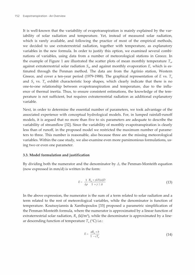
The formula contains three parameters, i.e. a (kg/kJ), b (kg/m2) and c (°C-1), to which a physi‐cal interpretation can be assigned. Since extraterrestrial solar radiation is the upper bound ofnet shortwave radiation, the dimensionless term a* = a / λρ represents the average percent‐age of the energy provided by the sun (in terms of Ra) and, after reaching the Earth’s terrain,is transformed to latent heat, thus driving the evapotranspiration process. Parameter blumps the missing information associated with aerodynamic processes, driven by the windand the vapour deficit in the atmosphere. Finally, the expression 1 – c Ta approximates themore complex 1 + γ΄ / Δ. We remind that γ΄ is function of the surface and aerodynamic re‐sistance (eq. 4) and Δ is the slope vapour pressure curve, which is function of Ta. As shownin Fig. 2, Ta and – (1 / Δ) are highly correlated, thus justifying the adoption of the linear ap‐proximation.

R2 = 0.9754

-1.8

-1.6

-1.4

-1.2

-1.0

-0.8

-0.6

-0.4

-0.2

0.0

0.0 5.0 10.0 15.0 20.0 25.0 30.0

Monthly temperature (oC)

- Inv

erse

of s

lope

vap

our

pres

sure

cur

ve

Figure 2. Scatter plot of Ta and – 1 / Δ (data from Agrinio station)

4. Application of the parametric formula over Greece

4.1. Meteorological data and computational tools

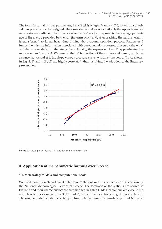
We used monthly meteorological data from 37 stations well-distributed over Greece, run bythe National Meteorological Service of Greece. The locations of the stations are shown inFigure 3 and their characteristics are summarized in Table 1. Most of stations are close to thesea. Their latitudes range from 35.0o to 41.5o, while their elevations range from 2 to 663 m.The original data include mean temperature, relative humidity, sunshine percent (i.e. ratio


153

of actual sunshine duration to maximum potential daylight hours per month) and wind ve‐locity records. These records cover the period 1968-1989 with very few missing values,which have not been considered in calculations. At all study locations, the monthly potentialevapotranspiration was calculated with the Penman-Monteith formula, assumed as refer‐ence model for the evaluation of the examined methodologies. The mean annual potentialevapotranspiration values, shown in Table 2, range from 912 mm (Florina station, NorthGreece, altitude 662 m) to 1628 mm (Ierapetra station, Crete Island, South Greece).

The handling of the time series and the related calculations were carried out using the Hy‐drognomon software, a powerful tool for the processing and management of hydrometeoro‐logical data [34]. The software is open-access and freely available at http://www.hydrognomon.org/.

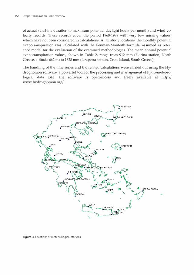
Figure 3. Locations of meteorological stations


No Station φ (o) z (m) No Station φ (o) z (m)

1 Agrinio 38.37 46 20 Larisa 39.39 74

2 Alexandroupoli 40.51 4 21 Limnos 39.54 17

3 Argostoli 38.11 2 22 Methoni 36.50 34

4 Arta 39.10 38 23 Milos 36.41 183

5 Chalkida 38.28 6 24 Mytiline 39.30 5

6 Chania 35.30 63 25 Naxos 37.60 9

7 Chios 38.20 4 26 Orestiada 41.50 48

8 Florina 40.47 662 27 Patra 38.15 3

9 Hellinico 37.54 15 28 Rhodes 36.24 37

10 Heracleio 35.20 39 29 Serres 41.40 35

11 Ierapetra 35.00 14 30 Siteia 35.12 28

12 Ioannina 39.42 484 31 Skyros 38.54 5

13 Kalamata 37.40 8 32 Thera 36.25 208

14 Kavala 40.54 63 33 Thessaloniki 40.31 5

15 Kerkyra 39.37 2 34 Trikala 39.33 116

16 Korinthos 38.20 15 35 Tripoli 37.32 663

17 Kozani 40.18 626 36 Volos 39.23 7

18 Kymi 38.38 221 37 Zakynthos 37.47 8

19 Kythira 36.10 167

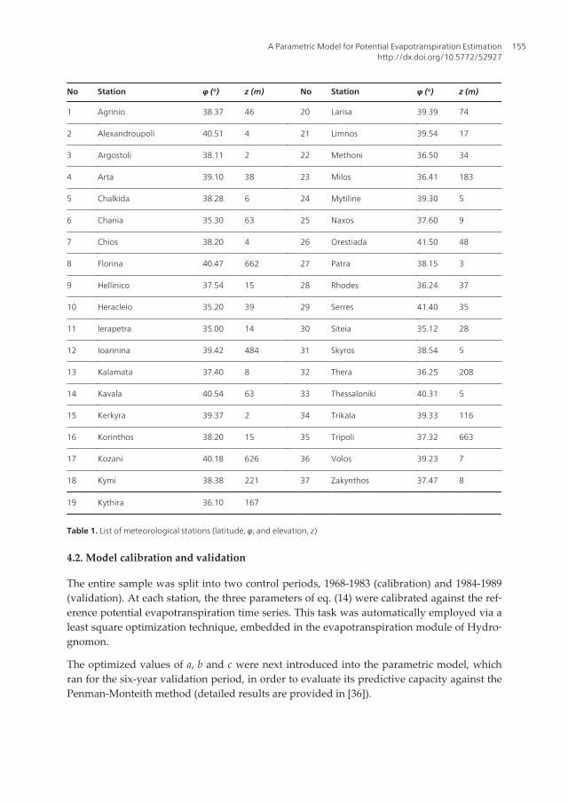
Table 1. List of meteorological stations (latitude, φ, and elevation, z)

4.2. Model calibration and validation

The entire sample was split into two control periods, 1968-1983 (calibration) and 1984-1989(validation). At each station, the three parameters of eq. (14) were calibrated against the ref‐erence potential evapotranspiration time series. This task was automatically employed via aleast square optimization technique, embedded in the evapotranspiration module of Hydro‐gnomon.

The optimized values of a, b and c were next introduced into the parametric model, whichran for the six-year validation period, in order to evaluate its predictive capacity against thePenman-Monteith method (detailed results are provided in [36]).


155

NoMAPET

(mm)>

CE

(cal.)

CE

(val.)No

MAPET

(mm)

CE

(cal.)

CE

(val.)

1 1108.4 0.989 0.975 20 1039.0 0.987 0.980

2 1164.0 0.971 0.970 21 1345.5 0.964 0.971

3 1277.9 0.982 0.980 22 1286.4 0.962 0.970

4 1195.0 0.981 0.871 23 1461.9 0.972 0.980

5 1274.5 0.950 0.953 24 1458.6 0.988 0.970

6 1296.0 0.973 0.963 25 1459.0 0.975 0.980

7 1412.9 0.919 0.953 26 1028.4 0.981 0.970

8 911.7 0.967 0.960 27 1205.4 0.987 0.960

9 1476.6 0.983 0.980 28 1551.9 0.972 0.970

10 1521.8 0.980 0.980 29 997.8 0.982 0.970

11 1628.4 0.962 0.940 30 1477.9 0.985 0.990

12 939.5 0.987 0.980 31 1297.9 0.926 0.910

13 1221.0 0.983 0.980 32 1437.1 0.971 0.940

14 962.4 0.983 0.980 33 1157.8 0.983 0.980

15 1089.5 0.989 0.990 34 1118.7 0.973 0.970

16 1483.1 0.957 0.820 35 1133.5 0.942 0.950

17 979.7 0.982 0.980 36 1240.6 0.981 0.910

18 1307.3 0.975 0.910 37 1370.4 0.974 0.980

19 1508.2 0.957 0.970

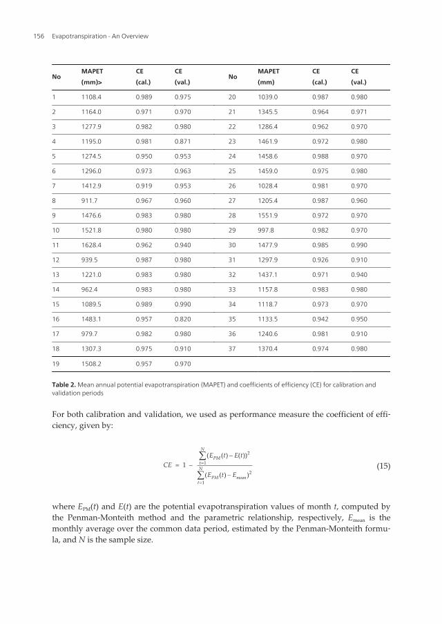
Table 2. Mean annual potential evapotranspiration (MAPET) and coefficients of efficiency (CE) for calibration andvalidation periods

For both calibration and validation, we used as performance measure the coefficient of effi‐ciency, given by:

2

1

2

1

( ( ) ( )) 1 –

( ( ) )

N

PMtN

PM meant

E t E tCE

E t E

=

=

-=

-

å

å(15)

where EPM(t) and E(t) are the potential evapotranspiration values of month t, computed bythe Penman-Monteith method and the parametric relationship, respectively, Emean is themonthly average over the common data period, estimated by the Penman-Monteith formu‐la, and N is the sample size.


The coefficients of efficiency for all stations, during the two control periods are given in Ta‐ble 2. For all stations the model fitting is very satisfactory, since the CE values are very high.Specifically, the average CE values of the 37 stations are 97.2% during calibration and 95.9%during validation, while their minimum values are 91.9 and 82.0%, respectively.

4.3. Comparison with other empirical methods

At all stations, we compared the performance of the parametric method (in terms of coeffi‐cients of efficiency) with two radiation-based approaches, i.e. the McGuiness model (eq. 7),and the generalized eq. (9), proposed by Oudin et al. [25]. In the latter, we applied the rec‐ommended values K1 = 100°C and K2 = 5°C. The distribution of the CE values for the twocontrol periods are summarized in Table 3. The suitability of the parametric model is obvi‐ous, while the other two methods exhibit much less satisfactory performance. Moreover, theimprovement of the empirical expression by Oudin et al. against the classical McGuinessmodel is rather marginal.

Parametric McGuiness Oudin et al.

CE Cal. Val. Cal. Val. Cal. Val.

>0.95 37 30 0 2 5 2

0.90-0.95 0 6 8 9 5 9

0.70-0.90 0 1 12 19 12 15

0.50-0.70 0 0 15 6 12 7

<0.50 0 0 2 1 3 4

Table 3. Distribution of CE values of radiation-based approaches

We also compared the performance of the new parametric approach against the most widelyused methods in Greece, i.e. Thornthwaite, Blaney-Criddle, and Hargreaves. We remindthat the first two are temperature-based, while the latter also uses extraterrestrial radiationand monthly average minimum and maximum temperature as inputs. The calculations ofmonthly potential evapotranspiration, using the Hydrognomon software, were made for tenrepresentative stations, with different climatic characteristics. For each station Table 4 givesthe coefficient of efficiency and the bias, i.e. the relative difference of the monthly averageagainst the average of the Penman-Monteith method (both refer to the entire control period1968-1988). The proposed formula is substantially more accurate, while all other commonlyused approaches do not provide satisfactory results across all locations. The suitability ofeach method depends on local conditions. Thus, at each location, one method may be satis‐factorily accurate, while another method may result to unacceptably large errors. In general,the Thornthwaite formula underestimates potential evapotranspiration by 30%, while theBlaney-Criddle method overestimates it by 30%. In stations that are far from the sea (Flori‐na, Larisa), the deviation exceeds 50%. The Hargreaves method, although it uses additionalinputs, totally fails to predict the potential evapotranspiration at some stations, resulting


157

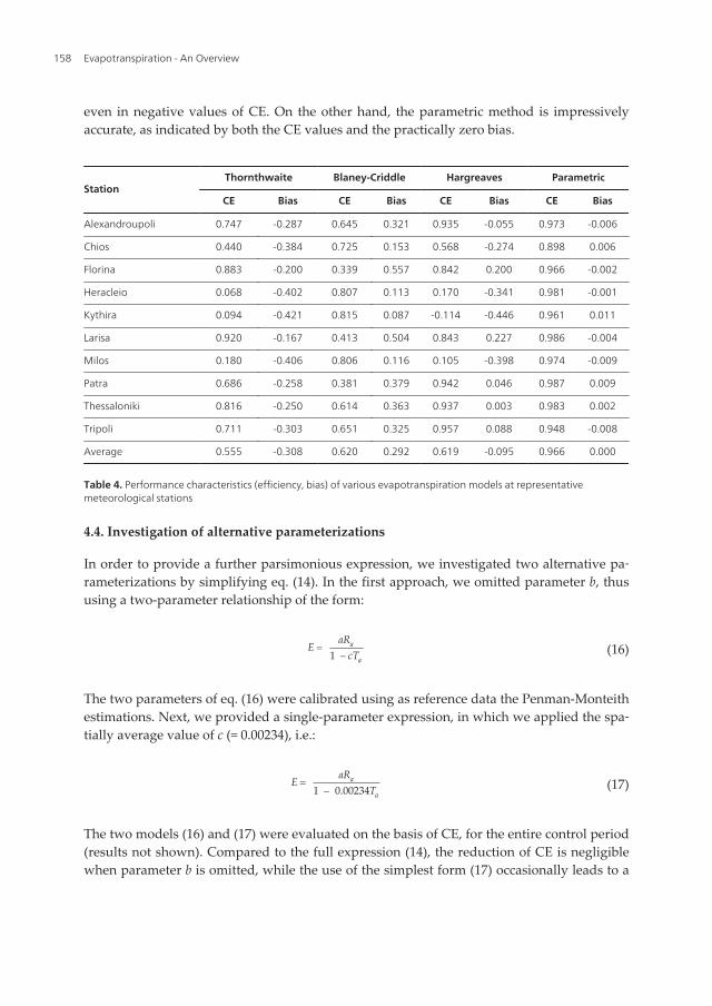
even in negative values of CE. On the other hand, the parametric method is impressivelyaccurate, as indicated by both the CE values and the practically zero bias.

StationThornthwaite Blaney-Criddle Hargreaves Parametric

CE Bias CE Bias CE Bias CE Bias

Alexandroupoli 0.747 -0.287 0.645 0.321 0.935 -0.055 0.973 -0.006

Chios 0.440 -0.384 0.725 0.153 0.568 -0.274 0.898 0.006

Florina 0.883 -0.200 0.339 0.557 0.842 0.200 0.966 -0.002

Heracleio 0.068 -0.402 0.807 0.113 0.170 -0.341 0.981 -0.001

Kythira 0.094 -0.421 0.815 0.087 -0.114 -0.446 0.961 0.011

Larisa 0.920 -0.167 0.413 0.504 0.843 0.227 0.986 -0.004

Milos 0.180 -0.406 0.806 0.116 0.105 -0.398 0.974 -0.009

Patra 0.686 -0.258 0.381 0.379 0.942 0.046 0.987 0.009

Thessaloniki 0.816 -0.250 0.614 0.363 0.937 0.003 0.983 0.002

Tripoli 0.711 -0.303 0.651 0.325 0.957 0.088 0.948 -0.008

Average 0.555 -0.308 0.620 0.292 0.619 -0.095 0.966 0.000

Table 4. Performance characteristics (efficiency, bias) of various evapotranspiration models at representativemeteorological stations

4.4. Investigation of alternative parameterizations

In order to provide a further parsimonious expression, we investigated two alternative pa‐rameterizations by simplifying eq. (14). In the first approach, we omitted parameter b, thususing a two-parameter relationship of the form:

1 –

a

a

aRE

cT= (16)

The two parameters of eq. (16) were calibrated using as reference data the Penman-Monteithestimations. Next, we provided a single-parameter expression, in which we applied the spa‐tially average value of c (= 0.00234), i.e.:

1 – 0.00234

a

a

aRE

T= (17)

The two models (16) and (17) were evaluated on the basis of CE, for the entire control period(results not shown). Compared to the full expression (14), the reduction of CE is negligiblewhen parameter b is omitted, while the use of the simplest form (17) occasionally leads to a


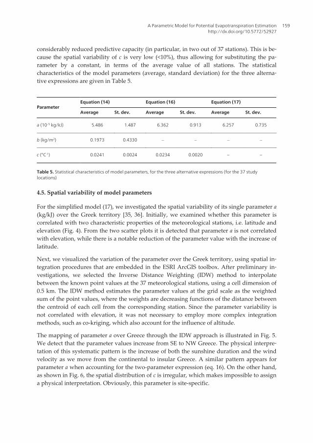
considerably reduced predictive capacity (in particular, in two out of 37 stations). This is be‐cause the spatial variability of c is very low (<10%), thus allowing for substituting the pa‐rameter by a constant, in terms of the average value of all stations. The statisticalcharacteristics of the model parameters (average, standard deviation) for the three alterna‐tive expressions are given in Table 5.

ParameterEquation (14) Equation (16) Equation (17)

Average St. dev. Average St. dev. Average St. dev.

a (10–5 kg/kJ) 5.486 1.487 6.362 0.913 6.257 0.735

b (kg/m2) 0.1973 0.4330 – – – –

c (°C-1) 0.0241 0.0024 0.0234 0.0020 – –

Table 5. Statistical characteristics of model parameters, for the three alternative expressions (for the 37 studylocations)

4.5. Spatial variability of model parameters

For the simplified model (17), we investigated the spatial variability of its single parameter a(kg/kJ) over the Greek territory [35, 36]. Initially, we examined whether this parameter iscorrelated with two characteristic properties of the meteorological stations, i.e. latitude andelevation (Fig. 4). From the two scatter plots it is detected that parameter a is not correlatedwith elevation, while there is a notable reduction of the parameter value with the increase oflatitude.

Next, we visualized the variation of the parameter over the Greek territory, using spatial in‐tegration procedures that are embedded in the ESRI ArcGIS toolbox. After preliminary in‐vestigations, we selected the Inverse Distance Weighting (IDW) method to interpolatebetween the known point values at the 37 meteorological stations, using a cell dimension of0.5 km. The IDW method estimates the parameter values at the grid scale as the weightedsum of the point values, where the weights are decreasing functions of the distance betweenthe centroid of each cell from the corresponding station. Since the parameter variability isnot correlated with elevation, it was not necessary to employ more complex integrationmethods, such as co-kriging, which also account for the influence of altitude.

The mapping of parameter a over Greece through the IDW approach is illustrated in Fig. 5.We detect that the parameter values increase from SE to NW Greece. The physical interpre‐tation of this systematic pattern is the increase of both the sunshine duration and the windvelocity as we move from the continental to insular Greece. A similar pattern appears forparameter a when accounting for the two-parameter expression (eq. 16). On the other hand,as shown in Fig. 6, the spatial distribution of c is irregular, which makes impossible to assigna physical interpretation. Obviously, this parameter is site-specific.


159

Figure 4. Scatter plots of parameter a (eq. 17) vs. latitude and elevation

Figure 5. Geographical distribution of parameter a (eq. 17) over Greece


Figure 6. Geographical distribution of parameter c (eq. 16) over Greece

5. Synopsis and discussion

A parametric, radiation-based model for the estimation of potential evapotranspiration hasbeen developed, which is parsimonious both in terms of data requirements and number ofparameters. Its mathematical expression originates from consecutive simplifications of thePenman-Monteith formula, thus being physically-consistent. In its full form, the model re‐quires three parameters to be calibrated. Yet, simpler formulations, with either one or twoparameters, were also examined, without significant degradation of the model performance.

The model parameters were optimized on the basis of monthly evapotranspiration data, es‐timated with the Penman-Monteith method at 37 meteorological stations in Greece, usinghistorical meteorological data for a 20-year period (1968-1988). The model exhibits excellentfitting to all locations. Its appropriateness is further revealed through extensive comparisonswith other empirical approaches, i.e. two radiation-based methods and three temperature-based ones. In particular, common temperature-based methods that have been widely usedin Greece provide rather disappointing results, while the new parametric model retains asystematically high predictive capacity across all study locations. This is the great advantageof parametric approaches against empirical ones, since calibration allows the coefficientsthat are involved in the mathematical formulas to be fitted to local climatic conditions.

The key model parameter was spatially interpolated throughout Greek territory, using atypical method in a GIS environment. The geographical distribution of the parameter exhib‐its a systematic increase from SE to NW, which is explained by the increase of sunshine du‐ration and wind velocity as we move from the continental to insular Greece. Similar patterns


161

were not found for the rest of model parameters. The practical value of this analysis is im‐portant, since it allows for establishing a specific formula for the estimation of potentialevapotranspiration at any point. Thus, a minimalistic model of high accuracy is now availa‐ble everywhere in Greece, which requires monthly temperature data as the only meteorolog‐ical input. The other inputs are the monthly extraterrestrial radiation, which is function oflatitude and time of the year, and a map of the parameter distribution.

To improve the model, it is essential to implement additional investigations, using a densernetwork of meteorological stations (especially stations in mountainous areas). In particular,it is necessary to examine the sensitivity of the various hydrometeorological variables thatare involved in the evapotranspiration process, and provide alternative formulations forvarious combinations of missing meteorological data.

Author details

Aristoteles Tegos, Andreas Efstratiadis and Demetris Koutsoyiannis

Department of Water Recourses & Environmental Engineering, School of Civil Engineering,National Technical University of Athens, Zographou, Greece

References

[1] Seckler D, Amarasinghe U, Molden D, de Silva R, Barker R. World Water Demandand Supply, 1990-2025: Scenarios and Issues. Research Report 19. International WaterManagement Institute, Colombo, Sri Lanka; 1998.

[2] Tsouni A, Contoes C, Koutsoyiannis D, Elias P, Mamassis N. Estimation of actualevapotranspiration by remote sensing: Application in Thessaly Plain, Greece. Sensors2008; 8(6): 3586–3600.

[3] Lhomme JP. Towards a rational definition of potential evaporation. Hydrology andEarth System Sciences 1997; 1: 257-264.

[4] Thornthwaite CW. An approach towards a rational classification of climate. Geo‐graphical Review 1948; 38: 55-94.

[5] Brutsaert W. Evaporation into the Atmosphere: Theory, History, and Applications,Springer; 1982.

[6] Lu J, Sun G, McNulty SG, Amatya DM. A comparison of six potential comparisonevapotranspiration methods for regional use in the South-eastern United States. Jour‐nal of the American Water Resources Association 2005; 41: 621–633.


[7] Allen RG, Pereira LS, Raes D, Smith M. Crop evapotranspiration: Guidelines forcomputing crop water requirements. FAO Irrigation and Drainage Paper 56, Rome;1998.

[8] Fisher JB, Whittaker RJ, Malhi Y. ET come home: Potential evapotranspiration in geo‐graphical ecology. Global Ecology and Biogeography 2011; 20(1): 1–18.

[9] Penman HL. Natural evaporation from open water, bare soil and grass. In: Proceed‐ings of the Royal Society of London 1948; 193: 120–145.

[10] Monteith JL. Evaporation and the environment: The state and movement of water inliving organism. XIXth Symposium. Cambridge University Press, Swansea; 1965.

[11] Allen RG, Jensen ME, Wright JL, Burman RD. Operational estimates of referenceevapotranspiration. Agronomy Journal 1989; 81: 650–662.

[12] Jensen ME, Burman RD, Allen RG. Evapotranspiration and irrigation water require‐ment. ASCE Manuals and Reports on Engineering Practice, 70; 1990.

[13] Mecham BQ. Scheduling turfgrass irrigation by various ET equations. Evapotranspi‐ration and irrigation scheduling. In: Proceedings of the Irrigation International Con‐ference. 3–6 November, San Antonio; 1996.

[14] Sentelhas PC, Gillespie TJ, Santos EA. Evaluation of FAO Penman-Monteith and al‐ternative methods for estimating reference evapotranspiration with missing data inSouthern Ontario, Canada. Agricultural Water Management 2010; 97(5): 635–644.

[15] Jensen M, Haise H. Estimating evapotranspiration from solar radiation. Journal ofthe Irrigation and Drainage Division. Proceedings of the ASCE 1963; 89(1R4): 15–41.

[16] McGuinness JL, Bordne EF. A comparison of lysimeter-derived potential evapotrans‐piration with computed values. Technical Bulletin 1452. Agricultural Research Serv‐ice, US Department of Agriculture, Washington, DC; 1972.

[17] Priestley CHB, Taylor RJ. On the assessment of surface heat fluxes and evaporationusing large-scale parameters. Monthly Weather Review 1972; 100: 81–92.

[18] Hargreaves GH, Samani ZA. Reference crop evaporation from temperature. AppliedEngineering in Agriculture 1985; 1(2) 96–99.

[19] Blaney HF, Criddle WD. Determining water requirements in irrigated areas from cli‐matological irrigation data. Technical Paper No. 96. US Department of Agriculture,Soil Conservation Service, Washington, DC; 1950.

[20] Linacre ET. A simple formula for estimating evaporation rates in various climates,using temperature data alone. Agricultural and Forest Meteorology 1977; 18: 409–424.

[21] Xu CY, Singh VP. Evaluation and generalization of radiation-based methods for cal‐culating evaporation. Hydrological Processes 2000; 14: 339–349.


163

[22] Xu CY, Singh VP. Evaluation and generalization of temperature-based methods forcalculating evaporation. Hydrological Processes 2001; 15: 305–319.

[23] Mamassis N, Efstratiadis A, Apostolidou E. Topography-adjusted solar radiation in‐dices and their importance in hydrology. Hydrological Sciences Journal 2012; 57(4):756–775.

[24] Shuttleworth WJ. Evaporation. In: Maidment DR. (ed.) Handbook of Hydrology,McGraw-Hill, New York; 1993: Ch. 4.

[25] Oudin L, Hervieu F, Michel C, Perrin C, Andréassian V, Anctil F, Loumagne C.Which potential evapotranspiration input for a lumped rainfall–runoff model? Part 2—Towards a simple and efficient potential evapotranspiration model for rainfall–runoff modelling. Journal of Hydrology 2004; 303(1–4): 290–306.

[26] Ward RC, Robinson M. Principles of Hydrology. 3rd edition, McGraw Hill, London;1989.

[27] Shaw EM. Hydrology in Practice. 3rd edition, Chapman and Hall, London; 1994.

[28] Doorenbos J, Pruit WO. Crop water requirements. Irrigation and Drainage Paper No24, FAO, Rome; 1977.

[29] Alexandris S, Kerkides P. New empirical formula for hourly estimations of referenceevapotranspiration. Agricultural Water Management 2003; 60(3): 157–180.

[30] Hounam CE. Problems of Evaporation Assessment in the Water Balance. Report onWMO/IHP Projects No. 13, World Health Organization, Geneva; 1971.

[31] Koutsoyiannis D. Seeking parsimony in hydrology and water resources technology.EGU General Assembly 2009, Geophysical Research Abstracts, Vol. 11, Vienna,11469, European Geosciences Union; 2009 (http://itia.ntua.gr/en/docinfo/906/).

[32] Wagener T, Boyle DP, Lees MJ, Wheater HS, Gupta HV, Sorooshian S. A frameworkfor development and application of hydrological models. Hydrology and Earth Sys‐tem Sciences 2001; 5(1): 13–26.

[33] Koutsoyiannis D, Xanthopoulos T. Engineering Hydrology, 3rd ed., National Techni‐cal University of Athens, Athens; 1999.

[34] Kozanis S, Christofides A, Mamassis N, Efstratiadis A, Koutsoyiannis D. Hydrogno‐mon – open source software for the analysis of hydrological data, EGU General As‐sembly 2010, Geophysical Research Abstracts, Vol. 12, Vienna, 12419, EuropeanGeosciences Union; 2010 (http://itia.ntua.gr/en/docinfo/962/).

[35] Tegos A. Simplification of evapotranspiration estimation in Greece. PostgraduateThesis. Department of Water Resources and Environmental Engineering – NationalTechnical University of Athens, Athens; 2007 (in Greek; http://itia.ntua.gr/en/docinfo/820/).


[36] Tegos A, Mamassis N, Koutsoyiannis D. Estimation of potential evapotranspirationwith minimal data dependence. EGU General Assembly 2009, Geophysical ResearchAbstracts, Vol. 11, Vienna, 1937, European Geosciences Union; 2009.


165

Documents

A Parametric Model for Potential Evapotranspiration Estimation