Embed Size (px)
Citation preview

Efficient Usage of Self ValidatedIntegrators for Space
Applications
Final Report
Authors: E.M. Alessi, A. Farrés, À. Jorba, C. Simó, A. VieiroAffiliation: University of Barcelona
ESA Researcher(s): T. Vinkó
Date:
Contacts:
Àngel JorbaTel: +34 934035734Fax: +34 934021601e-mail: [email protected] SummererTel: +31(0)715655174Fax: +31(0)715658018e-mail: [email protected]
Available on the ACT website http://www.esa.int/act
Ariadna ID: 07/5202Study Duration: 6 months
Contract Number: 20783/07/NL/CB

Efficient Usage of Self Validated Integrators
for Space Applications
Final Report
February 2008
Senior researchers: Angel Jorba, Carles Simo
Junior researchers: Elisa M. Alessi, Ariadna Farres, Arturo Vieiro
Departament de Matematica Aplicada i AnalisiUniversitat de Barcelona
Gran Via 585, 08007 Barcelona, Spain.
ESA Research Fellow / Technical Officer: Tamas Vinko
Ariadna ID: 07/5202Study duration: 6 months
Contract Number: 20783/07/NL/CB


Abstract
The present report addresses the possibilities offered by validated integrators to deal withsome space problems. First, we survey previous results on validated methods for ODEs andwe discuss their sharpness and efficiency, keeping in mind their suitability for space-relatedcomputations.
We have considered two concrete situations. The first one is the propagation of the orbit ofa NEO asteroid, starting from data affected by observational error for a moderate time span.We have focused on the concrete case of 99942 Apophis, which is having close approaches to theEarth on the years 2029 and 2037. The goal here is to check if the use of validated methods canbe useful to elucidate possible collisions of these objects with the Earth. The second problemconsidered is the transfer of a probe with low thrust propulsion from parking orbit around theEarth to a much higher orbit, including a capture by the Moon. The goal is to see how theuncertainties in the initial condition and the thrust affect the propagation of the orbit.


1
Contents
1 Introduction 3
1.1 Sources of errors . . . . . . . . . . . . . . . . . . . . . . . . . . . . . . . . . . . . 4
1.2 The Taylor method . . . . . . . . . . . . . . . . . . . . . . . . . . . . . . . . . . . 5
1.2.1 Automatic differentiation . . . . . . . . . . . . . . . . . . . . . . . . . . . 6
1.2.2 Estimation of order and step size . . . . . . . . . . . . . . . . . . . . . . . 8
1.2.3 Validated integration . . . . . . . . . . . . . . . . . . . . . . . . . . . . . . 8
1.3 Interval arithmetic . . . . . . . . . . . . . . . . . . . . . . . . . . . . . . . . . . . 8
1.3.1 Real interval arithmetic . . . . . . . . . . . . . . . . . . . . . . . . . . . . 91.3.2 Rounded interval arithmetic . . . . . . . . . . . . . . . . . . . . . . . . . . 10
1.3.3 The dependency problem and the wrapping effect . . . . . . . . . . . . . . 10
1.3.4 Software implementations for interval arithmetic . . . . . . . . . . . . . . 11
2 Applications 15
2.1 The two-body problem . . . . . . . . . . . . . . . . . . . . . . . . . . . . . . . . . 15
2.1.1 Local behaviour around an elliptic orbit . . . . . . . . . . . . . . . . . . . 152.2 Solar System models . . . . . . . . . . . . . . . . . . . . . . . . . . . . . . . . . . 16
2.2.1 The N -body problem . . . . . . . . . . . . . . . . . . . . . . . . . . . . . 17
2.2.2 The JPL model . . . . . . . . . . . . . . . . . . . . . . . . . . . . . . . . . 17
2.3 The orbit of a Near Earth Object (NEO) . . . . . . . . . . . . . . . . . . . . . . 18
2.4 The transfer of a probe using low-thrust . . . . . . . . . . . . . . . . . . . . . . . 19
3 Non validated methods 21
3.1 The N-body integrator . . . . . . . . . . . . . . . . . . . . . . . . . . . . . . . . . 21
3.1.1 Comparing the results with JPL 405 ephemerides . . . . . . . . . . . . . . 21
3.2 Precision and speed of the integrator . . . . . . . . . . . . . . . . . . . . . . . . . 23
3.3 Including Apophis . . . . . . . . . . . . . . . . . . . . . . . . . . . . . . . . . . . 24
3.3.1 Comparing the results with JPL 405 ephemerides . . . . . . . . . . . . . . 25
3.3.2 The non-rigorous propagation of an initial box . . . . . . . . . . . . . . . 26
3.3.3 The non-rigorous propagation of an initial box using variational equations 27
3.4 Low-Thrust . . . . . . . . . . . . . . . . . . . . . . . . . . . . . . . . . . . . . . . 28
3.4.1 Nominal orbits . . . . . . . . . . . . . . . . . . . . . . . . . . . . . . . . . 31
3.4.2 The non-rigorous propagation of an initial box using variational equations 33
4 Validated methods: theory 37
4.1 Interval based methods . . . . . . . . . . . . . . . . . . . . . . . . . . . . . . . . . 37
4.1.1 Moore’s direct algorithm . . . . . . . . . . . . . . . . . . . . . . . . . . . . 38
4.1.2 The parallelepiped method, the QR-Lohner method and new modifications 39
4.1.3 Cr-Lohner algorithms . . . . . . . . . . . . . . . . . . . . . . . . . . . . . 42
4.2 Taylor-based methods . . . . . . . . . . . . . . . . . . . . . . . . . . . . . . . . . 42
4.3 Subdivision strategy . . . . . . . . . . . . . . . . . . . . . . . . . . . . . . . . . . 44

2
5 Validated methods: results 45
5.1 Validated integration of Kepler’s problem . . . . . . . . . . . . . . . . . . . . . . 455.1.1 Second order interval methods . . . . . . . . . . . . . . . . . . . . . . . . 495.1.2 Subdivision strategy . . . . . . . . . . . . . . . . . . . . . . . . . . . . . . 50
5.2 Validated alternative to the rough enclosure . . . . . . . . . . . . . . . . . . . . . 515.3 Validated integration of the Apophis orbit . . . . . . . . . . . . . . . . . . . . . . 525.4 Validated integration of the low-thrust problem . . . . . . . . . . . . . . . . . . . 525.5 Summary . . . . . . . . . . . . . . . . . . . . . . . . . . . . . . . . . . . . . . . . 58
6 Conclusions and future work 59
6.1 Conclusions . . . . . . . . . . . . . . . . . . . . . . . . . . . . . . . . . . . . . . . 596.2 Future work . . . . . . . . . . . . . . . . . . . . . . . . . . . . . . . . . . . . . . . 626.3 Acknowledgements . . . . . . . . . . . . . . . . . . . . . . . . . . . . . . . . . . . 62
References 63
Appendixes
A N-body variationals, asteroid case 67
A.1 Set up and variational equations . . . . . . . . . . . . . . . . . . . . . . . . . . . 67A.2 A count on operations . . . . . . . . . . . . . . . . . . . . . . . . . . . . . . . . . 69A.3 On the optimal variational order to propagate a box . . . . . . . . . . . . . . . . 71A.4 On the integration of a finite jet . . . . . . . . . . . . . . . . . . . . . . . . . . . 72
A.4.1 Operation count . . . . . . . . . . . . . . . . . . . . . . . . . . . . . . . . 72
B Convergence and remainder 75

3
Chapter 1
Introduction
Many real life problems are well described by models consisting of Ordinary Differential Equa-tions (ODE),
dx
dt= f(t, x, λ),
where x belongs to some phase or states space E ⊂ Rn and λ, which accounts for the parameters
of the model, belongs to some parameter space P ⊂ Rp. Here we will focus on equations such
that the vector field f is given in closed form by means of analytic functions.
For most of the ODE the solutions to the Initial Value Problem (IVP) x(t0) = x0 are notknown in closed form or cannot be obtained by solving a simple equation, as happens, e.g., inthe case of the two-body problem which only requires the solution of Kepler’s equation.
For concreteness we denote the flow by ϕ, that is, given t0, x0, λ, the solution at a final timetf is denoted as
ϕ(tf ; t0, x0, λ).
This leads to the need of numerical integration of the IVP for ODE. Unfortunately allmethods are affected by the presence of integration errors at each step and by the propagationof errors by the proper dynamics.
In many critical applications, like the motion of a NEO or space missions using a close fly-byto a massive body, the effect of the errors can be critical. Hence, it is natural to ask for methodsproviding solutions which are as correct as possible and, better, to guarantee that the solutionat time tf is inside a given subset of the phase space. Furthermore this subset should be “small”,that is, the method should not overestimate its size.
On the other hand both initial data t0, x0 and the values of the parameters λ, are not exactlyknown. Consider, for instance, the case of a NEO a few days after it has been discovered (oreven at present time). Due to bad conditioning of initial observations the elements of its orbithave a large uncertainty. Hence, one should be able to give rigorous and sharp estimates of theset
ϕ(tf , t0,X0,Λ) = {ϕ(tf , t0, x0, λ), for all x0 ∈ X0, λ ∈ Λ} ,
where X0 and Λ are the sets which contain all possible initial values of x0, λ, respectively.
For conceptual simplicity, and without loss of generality, it is better to consider state andparameter variables together, that is, we can introduce
z =
(
xλ
)
,dz
dt=
(
f(t, z)0
)
,
where z ∈ EP = E × P, the state–parameter space. Also initial data can be considered in a setZ0 like X0 × Λ or a subset of it.

4 Chapter 1. Introduction
Different methods have been proposed to obtain rigorous estimates of Zf = ϕ(tf , t0, Z0)based on the use of interval analysis and generically known as “Self Validated Integrators” (seeChapter 4).
The three main points which should be taken carefully into account, when considering allthese methods and applications are:
a) Rigorous estimates should be provided.
b) The estimates should be sharp, that is, not producing a too large image domain.
c) They should be efficient from a CPU time point of view.
1.1 Sources of errors
The numerical integration of ODE is a key task in many applications. In this work we havebeen concerned with conservative systems, e.g., given by some Hamiltonian function, or close toconservative systems. In contrast to some dissipative systems having simple global attractors(like steady states or periodic solutions) the effect of the errors introduced by the numericalmethod can invalidate the numerically obtained solution.
One should distinguish clearly between regular and chaotic orbits. The difference in be-haviour can be measured by means of the Lyapunov exponents (see, e.g. [Sim01]). Theymeasure the exponential rate of separation of nearby orbits. We can consider as regular theorbits for which the maximal Lyapunov exponent is zero and then nearby orbits separate in apotential way (typically in a linear way) with respect to time. Otherwise, orbits for which themaximal Lyapunov exponent is positive can be considered as chaotic or with strong sensitivityto initial conditions.
One should note, however, that Lyapunov exponents are defined as a limit of the exponentialrate of separation when time tends to infinity. In practice time will be finite and the orbit onlyexplores a reduced part of the phase space. It is better to refer to some kind of local Lyapunovexponent where local refers to the fact that the orbits we can be interested in move only on areduced subset of the available phase space.
Numerical integration of ODE is affected by different kinds of errors:
1. Errors in the initial data, x0,
2. Errors in the model, for instance in the parameters λ describing the model,
3. Truncation errors due to the fact that the numerical method, even if computations weredone with infinite precision, is just an approximation, depending on the order of themethod,
4. Round off errors due to the fact that computations are done with a finite number of digits,
5. Propagation of the errors produced in the different steps due to the proper characteristicsof the dynamics. This is specially critical in the case of chaotic orbits.
It is clear that the effect of items 3. and 4. can be decreased by high order methods and,if required, by doing computations with more digits (e.g., with quadruple precision or higher).But one should face the problems due to items 1. and 2. Concerning item 5. it is possible, insome cases, to decrease its effect by a suitable reformulation of the problem (e.g., using someregularising variables like KS variables for close approaches in perturbed two-body problems,see [SS71]).

1.2. The Taylor method 5
In any case, a reasonable method should behave in a nice way if we consider the evolutionof the theoretically preserved quantities, such as energy, momentum, etc.
Furthermore, it is also clear that to cope with item 5 a validated method requires information,at least, on the first variational equations. This allows to bound the derivatives of the final statewith respect to the initial one (and also with respect to the parameters, of course). Theseequations are used for the computation of Lyapunov exponents. They allow to detect if theorbit behaves in a regular or chaotic way, which is relevant, even at a local scale, to decide aboutthe more convenient set of variables to be used.
The strong relation between propagation of errors and dynamical behaviour of system athand must necessarily be taken into account.
1.2 The Taylor method
Consider the initial value problem
{
x′(t) = f(t, x(t)),x(a) = x0,
(1.1)
where f is assumed to be analytic on its domain of definition, and that x(t) is assumed to bedefined for t ∈ [a, b]. We are interested in approximating the function x(t) on [a, b]. The ideaof the Taylor method is very simple: given the initial condition x(t0) = x0 (t0 = a), the valuex(t0 + h0) is approximated from the Taylor series of the solution x(t) at t = t0,
x0 = x(t = 0),
xm+1 = xm + x′(tm)hm +x′′(tm)
2!h2
m + · · · + x(p)(tm)
p!hp
m, m = 0, . . . ,M − 1,(1.2)
where tm+1 = tm + hm, hm > 0 and tM = b.
For a practical implementation one needs an effective method to compute the values of thederivatives x(j)(tm). A first procedure to obtain them is to differentiate the first equation in(1.1) w.r.t. t, at the point t = tm. Hence,
x′(tm) = f(tm, x(tm)), x′′(tm) = ft(tm, x(tm)) + fx(tm, x(tm))x′(tm),
and so on. Therefore, the first step to apply this method is, for a given f , to compute thesederivatives up to a suitable order. Then, for each step of the integration (see (1.2)), we haveto evaluate these expressions to obtain the coefficients of the power series of x(t) at t = tm.Usually, these expressions will be very cumbersome, so it will take a significant amount of timeto evaluate them numerically. This, jointly with the initial effort to compute the derivatives off , is the main drawback of this approach for the Taylor method.
This difficulty can be overcome by means of the so-called automatic differentiation (see[BKSF59], [Wen64], [Moo66], [Ral81], [GC91], [BCCG92], [BBCG96], [Gri00]). This is a proce-dure that allows for a fast evaluation of the derivatives of a given function, up to arbitrarily highorders. As far as we know, these ideas were first used in Celestial Mechanics problems ([Ste56],[Ste57]; see also [Bro71]).
We note that the algorithm to compute these derivatives by automatic differentiation hasto be coded separately for different systems. This coding can be either done by a human(see, for instance, [Bro71] for an example with the N -body problem) or by another program(see [BKSF59, Gib60, CC94, JZ05] for general-purpose computer programs). An alternativeprocedure to apply the Taylor method can be found in [SV87] and [IS90]. We can also find somepublic domain software to generate numerical integrators of ODEs using Taylor methods:

6 Chapter 1. Introduction
• ATOMFT, http://www.eng.mu.edu/corlissg/FtpStuff/Atom3_11/. ATOMFT is writtenin Fortran 77 and it reads Fortran-like statements of the system of ODEs and writes aFortran 77 program that is run to solve numerically the system using Taylor series.
• taylor. It can be obtained from http://www.maia.ub.es/~angel/taylor/. It reads afile with a system of ODEs and it outputs a time-stepper for it (in C/C++), with automaticselection of order and step size. Several extended precision arithmetics are supported.
There is also a public domain package for automatic differentiation, ADOL-C, included as anoption in many Linux distributions (home page: http://www.math.tu-dresden.de/~adol-c/).It facilitates the evaluation of first and higher derivatives of vector functions that are defined bycomputer programs written in C or C++.
There are several papers that focus on computer implementations of the Taylor method indifferent contexts; see, for instance, [BWZ70], [CC82], [CC94] and [Hoe01]. A good survey is[NJC99] (see also [Cor95]).
1.2.1 Automatic differentiation
As it has been mentioned before, automatic differentiation is a recursive procedure to computethe value of the derivatives of certain functions at a given point (relevant references are [Moo66,Ral81, Gri00]). The functions considered are those that can be obtained by sum, product,quotient, and composition of elementary functions (elementary functions include polynomials,trigonometric functions, real powers, exponentials and logarithms). We note that the vectorfields used in Celestial Mechanics and Astrodynamics belong to this category. Other functionscan be considered as elementary if they are defined as the solution of some differential equationwhose coefficients are previously known to be elementary functions. A notorious case of a non-elementary function is Γ(x). A celebrated theorem of Holder states that Γ does not satisfy anyalgebraic differential equation whose coefficients are rational functions.
Assume that a is a real function of a real variable t.
Definition 1.2.1 The normalised j-th derivative of a at the point t is
a[j](t) =1
j!a(j)(t).
Assume now that a(t) = F (b(t), c(t)) and that we know the values b[j](t) and c[j](t), j =0, . . . , n, for a given t. The next proposition gives the n-th derivative of a at t for some functionsF .
Proposition 1.2.1 If the functions b and c are of class Cn, and α ∈ R \ {0}, we have
1. If a(t) = b(t) ± c(t), then a[n](t) = b[n](t) ± c[n](t).
2. If a(t) = b(t)c(t), then a[n](t) =
n∑
j=0
b[n−j](t)c[j](t).
3. If a(t) =b(t)
c(t), then a[n](t) =
1
c[0](t)
b[n](t) −n
∑
j=1
c[j](t)a[n−j](t)
.
4. If a(t) = b(t)α, then a[n](t) =1
nb[0](t)
n−1∑
j=0
((n − j)α − j) b[n−j](t)a[j](t).
5. If a(t) = eb(t), then a[n](t) =1
n
n−1∑
j=0
(n− j) a[j](t)b[n−j](t).

1.2. The Taylor method 7
6. If a(t) = ln b(t), then a[n](t) =1
b[0](t)
b[n](t) − 1
n
n−1∑
j=1
(n− j)b[j](t)a[n−j](t)
.
7. If a(t) = cos c(t) and b(t) = sin c(t), then
a[n](t) = − 1
n
n∑
j=1
jb[n−j](t)c[j](t), b[n](t) =1
n
n∑
j=1
ja[n−j](t)c[j](t).
It is possible to derive similar formulas for other functions, like inverse trigonometric func-tions.
We note that the number of arithmetic operations to evaluate the normalised derivatives ofa function up to order n is O(n2). We will come back to this point later on.
As an example, we can apply them to the Van der Pol equation,
x′ = y,y′ = (1 − x2)y − x.
}
(1.3)
To this end we decompose the right-hand side of these equations in a sequence of simple opera-tions:
u1 = x,u2 = y,u3 = u1u1,u4 = 1 − u3,u5 = u4u2,u6 = u5 − u1,x′ = u2,y′ = u6.
(1.4)
Then, we can apply the formulas given in Proposition 1.2.1 (items 1 and 2) to each of the
equations in (1.4) to derive recursive formulas for u[n]j , j = 1, . . . , 6,
u[n]1 (t) = x[n](t),
u[n]2 (t) = y[n](t),
u[n]3 (t) =
n∑
i=0
u[n−i]1 (t)u
[i]1 (t),
u[n]4 (t) = −u[n]
3 (t), n > 0
u[n]5 (t) =
n∑
i=0
u[n−i]4 (t)u
[i]2 (t),
u[n]6 (t) = u
[n]5 (t) − u
[n]1 (t),
x[n+1](t) =1
n+ 1u
[n]2 (t),
y[n+1](t) =1
n+ 1u
[n]6 (t).
The factor 1n+1 in the last two formulas is because we are computing normalised derivatives.
Then, we can apply recursively these formulas for n = 0, 1, . . ., up to a suitable degree p, toobtain the jet of normalised derivatives for the solution at a given point of the ODE. Note thatis not necessary to select the value of p in advance.

8 Chapter 1. Introduction
1.2.2 Estimation of order and step size
There are several possibilities to estimate an order and step size for the Taylor method. WhenTaylor is used in a non-validated way, these estimates come from the asymptotic behaviour ofthe error. The following result can be found in [Sim01].
Proposition 1.2.2 Assume that the function z 7→ x(tm + z) is analytic on a disk of radius ρm.Let Am be a positive constant such that
|x[j]m | ≤ Am
ρjm
, ∀ j ∈ N, (1.5)
and assume that the dominant part in the computational cost is proportional to the square of theorder up to which the Taylor series is computed. Then, if the required accuracy ε tends to 0, thevalues of hm (local step) and pm (local order) that give the required accuracy and minimise theglobal number of operations tend to
hm =ρm
e2and pm = −1
2ln
(
ε
Am
)
− 1. (1.6)
Note that the optimal step size does not depend on the level of accuracy. The optimal orderis, in fact, the order that guarantees the required precision once the step size has been selected.
It is important to note that the values (1.6) are optimal only when the bound (1.5) cannotbe improved. If the value Am can be reduced –or if the function x(t) is entire– the previousvalues are not optimal in the sense that a larger hm and/or a smaller pm could still deliver therequired accuracy.
1.2.3 Validated integration
Validated methods are numerical methods based on an “exact” arithmetic, combined with arigorous estimate of the truncation errors. Hence, the results (usually values with bounds onthe error) are rigorous. For an “exact” arithmetic we mean a validated floating point arithmetic,which is usually an interval arithmetic, that guarantees that the result is between the givenbounds (see Section 1.3).
One of the advantages of validated methods is that they produce rigorous results, that canbe used to derive computer-assisted proofs of theorems (see, for instance, [Lan82, EKW84]). Ifthe computation requires the numerical integration of a non-stiff ODE, then Taylor method isprobably the best choice to have a rigorous estimation of the error.
In these cases, it is quite common to use a high precision arithmetic to check the conditionsneeded to derive the computer assisted proof. For instance, [KS07] shows the linear stabilityof the Figure Eight solution of the 3-body problem, by using an extended precision arithmetic(100 digits) and computing this orbit and its first variationals up to a very high accuracy. Thisallows for a very precise validated integration which, in turn, allows to complete the proof.
The situation considered in this work is of a different nature. We are focusing on spaceapplications (propagating the motion of an asteroid or a spacecraft), and this means that thereis an error in the data that cannot be reduced by extending the accuracy of the arithmetic.Because of the relatively large size of these errors, it will be enough to use interval arithmeticsbased on the double precision of the computer.
1.3 Interval arithmetic
Interval arithmetic was first introduced by E. Moore [Moo66] in 1966. In this book the foun-dations of interval arithmetic where laid. In the past years, it has been developed being now
1.3. Interval arithmetic 9
a very important tool for the computation of rigorous bounds for many problems in numericalanalysis. See, for instance, [Zgl07] for a description of different applications.
We define the set of intervals on the real line as:
IR = {[a] = [al, au] | al, au ∈ R, al ≤ au}.
An interval number [a] is the set of real numbers x that satisfy al ≤ x ≤ au. If al = au wesay that we have a point interval and if al = −au we say that we have a symmetric interval.Two intervals [a], [b] are equal iff al = bl and au = bu.
We can define the classical inclusions as follows, we will say that [a] ⊆ [b] iff al ≤ bl ≤ bu ≤ au.And we can also define the partial ordering as [a] < [b] iff au < bl.
We can also define the following quantities:
• w([a]) = au − al is the width of the interval [a].
• m([a]) = (al + au)/2 is the mid point of the interval [a].
• |[a]| = max(|al|, |au|) is the magnitude of the interval [a].
1.3.1 Real interval arithmetic
The interval arithmetic is an extension of the real arithmetic. We will first assume that theend points of the intervals can be computed in an exact way. Further on we will discuss whichmodifications must be done so that the round-off errors are taken into account.
Let [a] and [b] ∈ IR and ◦ ∈ {+,−, ∗, /} be one of the arithmetic operations. We define thearithmetic operation on intervals as:
[a] ◦ [b] = {x ◦ y | x ∈ [a], y ∈ [b]}, (1.7)
where, for ◦ = / the operation is not defined if 0 ∈ [b]. It is immediate to see that:
• [a] + [b] = [al + bl, au + bu],
• [a] − [b] = [al − bu, au − bl],
• [a] ∗ [b] = [min(albl, albu, aubl, aubu),max(albl, albu, aubl, aubu)],
• [a]/[b] = [al, au] ∗ [1/bu, 1/bl], if bl > 0.
Properties:
1. The interval addition and multiplication are both associative and commutative, i.e. if[a], [b] and [c] ∈ IR, then:
[a] + ([b] + [c]) = ([a] + [b]) + [c],
[a] + [b] = [b] + [a],
[a] ∗ ([b] ∗ [c]) = ([a] ∗ [b]) ∗ [c],
[a] ∗ [b] = [b] ∗ [a].
2. The real numbers 0 and 1 are identities for the interval addition and multiplication re-spectively, i.e. if [a] is an interval then:
0 + [a] = [a] + 0 = [a],
1 ∗ [a] = [a] ∗ 1 = [a].

10 Chapter 1. Introduction
3. The inverse elements for addition and for multiplication only exist in the degenerate case,i.e. for point intervals.
4. The arithmetic operations are monotonic inclusions, i.e. if [a1] ⊂ [a2] and [b1] ⊂ [b2] then:
[a1] ◦ [b1] ⊂ [a2] ◦ [b2], where 0 /∈ [b2] if ◦ = /.
5. The distributive law does not always hold for interval arithmetic, but we do have the subdistributive law, i.e. if [a], [b] and [c] ∈ IR, then
[a] ∗ ([b] + [c]) ⊆ [a] ∗ [b] + [a] ∗ [c].
It can be seen that the distributive law holds if [b] ∗ [c] ≥ 0, if [a] is a point interval or ifboth [b] and [c] are symmetric.
We will refer to an interval vector and interval matrix as a vector or matrix where all theircomponents are intervals. And we will define the set of n-dimensional real interval vectors asIR
n and the set of n×m-dimensional real interval matrices as IRn×m. The interval arithmetic
operations involving interval vectors and interval matrices are defined as in the scalar case butsubstituting the scalars by intervals and using the definitions seen above. Further propertiesof the interval arithmetic on interval vectors and matrices and the extension of the intervalarithmetic to other functions can be seen in [Moo66, Moo79, AH83].
1.3.2 Rounded interval arithmetic
The interest in interval arithmetic has aroused, specially due to the limitations of the represen-tation of floating point numbers on a computer. Every time that a real number x is stored on acomputer or that computations with such numbers are made, round-off errors occur. Roundedinterval arithmetic provides a tool to bound the roundoff error in an automatic way.
Now, instead of representing the real number x by a machine number, it will be representedby an interval [x] = [xH, xN], where xH is the negative rounding of x and xN is the positiverounding of x. Then we can use the real interval arithmetic described before but roundingpositive on the right end points and rounding negative on the left end points, i.e. if [a] = [al, au]and [b] = [bl, bu] are intervals, with the endpoints previously rounded positive and negative asneeded, and ◦ = {+,−, ∗, /}, then:
• [a] + [b] = [(al + bl)H, (au + bu)N],
• [a] − [b] = [(al − bu)H, (au − bl)N],
• [a] ∗ [b] = [min(albl, albu, aubl, aubu)H,max(albl, albu, aubl, aubu)N],
• [a]/[b] = [al, au] ∗ [1/bu, 1/bl], if bl > 0.
On our validated computations we will use a rounded interval arithmetic instead of the realinterval arithmetic. In this way, after all the computations, we will have an interval that containsthe exact result.
1.3.3 The dependency problem and the wrapping effect
As it was observed by E. Moore [Moo66], interval arithmetic is sometimes affected by overesti-mation due to the dependency problem, which happens as interval arithmetic cannot detect thedifferent occurrences on the same variable.

1.3. Interval arithmetic 11
Figure 1.1: The fields in a double variable, according to the standard IEEE 754
For instance, x− x = 0 for all x ∈ [1, 2], but using interval arithmetic we have that [1, 2] −[1, 2] = [−1, 1]. It is true that the true solution [0, 0] is contained in [−1, 1], but we havea big overestimation. Another example would be x2 − x for x ∈ [0, 1]. It can be seen thatfor all x ∈ [0, 1], (x2 − x) ∈ [−1/4, 0]. Note that using interval arithmetic we have [0, 1] ∗[0, 1] − [0, 1] = [−1, 1]. Notice that x2 − x = x(x− 1) and if we evaluate this second expression:[0, 1]∗([0, 1]−1) = [−1, 0], we get a better estimation of the real interval. So here we can see twoclear examples of the dependency on the order of the operations that occur in interval arithmetic.This is a situation that must be taken into account in order to get accurate estimations of thereal result. A correct estimate of f([a, b]) for continuous functions would require to find extremaof f on [a, b]. In general, this cannot be achieved quickly, specially in the case of several variables.Anyway, subdivision algorithms can improve the result. In the x 7→ x2 −x example, subdivisionin 10 equal parts gives the result [−0.35, 0.1].
Another source of error in interval arithmetics is the wrapping effect. Let us consider the
function: f(x, y) =√
22 (x + y, y − x). The image of the square: [0,
√2] × [0,
√2] is the rotated
square of corners (0, 0), (1,−1), (2, 0) and (1, 1), but interval arithmetic gives [0, 2] × [−1, 1], asquare that doubles the size.
These and other examples have been studied by E. Moore [Moo66] and other authors, forinstance [NJ01]. In this project, we will describe techniques that can be developed in order todeal with these two effects in an accurate way, and to get good approximations of the real result.
1.3.4 Software implementations for interval arithmetic
There are several possibilities to construct an interval arithmetic. Usually, an interval arithmeticis defined as a structure with two members, the upper and the lower bounds of the interval.These members are floating point types. Depending on the considered application, they can bedouble precision numbers, or to have extended precision.
In this work, due to the fairy large amount of error in the initial data, and to the relativelymoderate number of floating point operations in the experiments done so far, we have chosento use an arithmetic based on the standard double precision of the computer: using extendedarithmetic makes the programs slower without any significant gain in accuracy.
There are several libraries in the public domain for interval arithmetic. For a comprehensivelist, see http://www.cs.utep.edu/interval-comp/intsoft.html. As it has been mentionedabove, we will only focus on arithmetics based on the standard double precision. In the nextsections we discuss several possibilities to implement such arithmetic.
Accessing the internal representation
There is a widely accepted standard to store floating point numbers, the IEEE Standard forBinary Floating-Point Arithmetic (IEEE 754). In short, floating point numbers are stored usingone bit for the sign, 11 bits for the exponent, and 52 bits for the mantissa (for a discussion see,for instance, [Gol91]). This has been represented schematically in Figure 1.1

12 Chapter 1. Introduction
The idea is, after each arithmetic operation, to access the bit representation of the result andto add (or subtract) 1 to the less significant bit to produce an enclosure for the true result. Thistechnique has been used in the libraries FI LIB (ANSI C) and FILIB++ (C++), freely accessiblefrom http://www.math.uni-wuppertal.de/~xsc/software/filib.html. More details can befound in [LTWVG+06].
Using the rounding modes of the processor
A second possibility is provided by the rounding modes specified by the standard IEEE 754:round to nearest (the default), round toward 0, round toward +∞, and round toward −∞. Forinstance, if we are adding two intervals it is enough to add the lower bounds with roundingtoward −∞ and the upper bounds with rounding toward +∞.
The GCC compiler on Intel platforms provides library functions to access and modify therounding modes of the processor. We have implemented a first version of an interval arithmeticbased on the use of these rounding modes. The main drawback is that every time the roundingmode is altered, the floating point pipeline is restarted which means a considerable loss ofperformance of the floating point unit.
Correcting the output of the operations
We have considered a third possibility: assuming that the result of each arithmetic operation iscorrect up to rounding error, we can modify the result of the operation up and down to obtain anenclosure for the true result (as it is done in the FI LIB and FILIB++ libraries). The difference isthat, instead of accessing the bits of the mantissa of the floating point variable (which is costlyin time), we multiply by a correcting factor. For instance, if a = b+ c > 0, we can construct theupper and lower bounds by doing a = a(1 − δ) and a = a(1 + ε), for suitable positive constantsε and δ. It is clear that ε and δ have to be as small as possible to minimise the growing of thesize of the intervals, but if they are too small the rounding of the computer arithmetic makesthat a = a = a, and the result will be wrong.
We have selected the values ε = 2−52 (the so-called machine epsilon) and δ = 2−53 (half ofthe machine epsilon). The reason for using this δ comes from the way the subtraction (and thesubsequent rounding) is done.
In the implementation (in C++) we have added a flag to optionally ask for verification ofthe result after each operation. This verification consists in checking the condition a < a < a,which means that we have obtained an enclosure for the result. A particular point that has tobe considered here is the effect of the extra digits that the Intel CPU has in its floating pointregisters (80 bits each). Think of the following situation:
a) the code generated by the compiler is keeping the variables in these extra precision registersso that the relation a < a < a is verified inside those registers;
b) once these numbers are stored in memory (only 64 bits), the roundoff makes that a = aor a = a.
This checking is done by accessing the bit representation of the floating point number (8 bytes),using a union type variable to overlap the number with two integer variables (4 bytes each). Inthis way, the checking is done in a very fast way: the check slows down the arithmetic by a 30%.We have done this check on a set of 1010 randomly chosen double precision numbers and thecondition has been satisfied in all the cases. A second test has been to use the flag -ffloat-storeof the GCC compiler when compiling the code that checks for the condition a < a < a: this flagforces that, after each arithmetic operation, the result is stored in memory (64 bits). In thisway, we have ruled out the previous effect when checking the previous inequalities. This secondtest slows down a lot the arithmetic.
1.3. Interval arithmetic 13
Comparisons
We have done several comparison bewtween these arithmetics. We only explain one of the tests,which is enough to give an idea of how they compare. This test is the scalar product of twoarrays of interval type, of 1000 components each. To have a measurable time, this productis done 106 times. As a reference, this test takes about 4.4 seconds using the double precisionarithmetic of the computer (a Linux workstation with a 3.2GHz Intel Xeon CPU). The sametest using our library takes 24.8 seconds, and using FI LIB it takes 108.4 seconds. For this testwe have compiled the FI LIB library with the -O3 option, although the makefile that comes withthe source of the library does not use any optimization flag.
Other options
There are other options to construct a fast interval arithmetic. For instance, instead of storingthe upper and lower bountd for the interval, we can store the central point and the radius. Then,the operations are done using the central point of the intervals (using the standard floating pointarithmetic) and the resulting radius is modified to account for the roundoff of the operation.We have not explored this possibility in this work, but it is an interesting option that we planto consider in the future.

14 Chapter 1. Introduction

15
Chapter 2
Applications
The aim of this work is to develop validated methods that can be applied to space relatedproblems. We have chosen two particular examples where we will apply these methods. Thefirst one is the propagation of the orbit of a Near Earth Object (NEO) and the second one isa low thrust transfer of a probe from a neighbourhood of the Earth to a neighbourhood of theMoon. In both problems we have an uncertainty in the initial condition and we want to knowthe effect of these uncertainties after a long time. They also require a long time integration thatmust be done in an accurate way. In this section, we will briefly describe these two applications.
2.1 The two-body problem
A first approximation of the motion of an asteroid orbiting around the Sun or of a probe thatorbits around the Earth is the well-known two-body problem (details can be found in almostany textbook on Classical or Celestial Mechanics, e.g. [Mou14, Pol76, Dan88]). We will use thisproblem as a toy model to test the validated techniques that have been developed. This is donedue to the simplicity of this model and because we have a complete knowledge of the solutionsof the problem.
The two-body problem describes the motion of two point masses X1 and X2 ∈ R3 of masses
m1 and m2, respectively, that are evolving under their mutual gravitational attraction. Thisproblem can be reformulated by taking r = X1 −X2, namely,
r = −µ r
‖r‖3, (2.1)
where µ = G(m1 +m2) is the mass parameter and G is the gravitational constant.The above system is super integrable, that is, it has more first integrals than degrees of
freedom. In particular, the first integral of the energy can be defined as
E =v2
2− µ
r, (2.2)
where v represents the velocity of the second body with respect to the first one.In our tests, we will consider that one of the particles is massless. This is the most natural
assumption when one considers the motion of an asteroid around the Sun or of a low-thrustprobe in the Earth-Moon system. We notice that this hypothesis reduces the problem to acentral vector field in the asteroid case.
2.1.1 Local behaviour around an elliptic orbit
We are interested in the numerical propagation of an uncertainty in position and, as first ap-proximation, Kepler’s third law gives how such error is propagated.

16 Chapter 2. Applications
We recall that this reads
n2a3 = µ, (2.3)
where n and a are, respectively, the mean motion and the semi-major axis associated with agiven orbit. Roughly speaking, if we consider two orbits characterised by different values of a,say a1 > a2, then Eq. (2.3) yields T1 > T2, where Ti = 2π/ni (i = 1, 2) is the correspondingperiod. This means that on the first orbit a particle will move slower than on the second one.
We can apply the above argument to predict the behaviour of a set of initial conditions whichare displaced one from the other in position. This displacement results in an uncertainty onthe semi–major axis, say ∆a, which makes the mean motion n to vary in a quantity ∆n. Moreprecisely, expanding Eq. (2.3) up to first order, we have
2na3∆n+ 3a2n2∆a = 0. (2.4)
We can always rescale the variables of the problem in such a way that µ = 1, n0 = 1 (i.e.T0 = 2π) and a0 = 1, where the subindex 0 refers to a nominal initial condition. In this way,any initial condition associated with ai = a0 + ∆a = 1 + ∆a will be characterised by
ni = n0 + ∆n = 1 − 3
2∆a.
After m revolutions of the nominal orbit, the others will be delayed by an angle ∆ψ given by
∆ψ = −3
2mT0∆a = −3mπ∆a ≈ −10m∆a.
As a consequence, if we integrate numerically a random set of initial conditions, we will see thebox stretching out along the orbit, that is, at a given time different points displaced one aheadthe other.
Let us consider two vectors, one tangent to the orbit and the other orthogonal to it at theinitial time. After m revolutions, the angle α between them will have changed according to
tan (α) =∆a
∆ψ≈ 1
10m.
For m large enough, we have
α ≈ 1
10m.
Moreover, the stretching of the box behaves linearly, in a first approximation, with respectto the time t. This can be proved noting that in action-angle variables, I and ϕ, the angle ϕevolves linearly with time, depending only on the constant action. Since this change of variablesis a diffeomorphism, the same behaviour is observed approximately in Cartesian coordinates ifwe approximate locally the diffeomorphism by its differential map.
2.2 Solar System models
As we want to describe the motion of an object in space, we first need to have a good modelof the motion of the Solar System. It is well known that the motion of the planets can beapproximated by the N -body problem.

2.2. Solar System models 17
Body/Planet G ·mMercury 0.4912547451450812 × 10⁻¹⁰
Venus 0.7243452486162703 × 10⁻⁹
Earth 8.8876923901135099 × 10⁻¹⁰
Mars 0.9549535105779258 × 10⁻¹⁰
Jupiter 0.2825345909524226 × 10⁻⁶
Saturn 0.8459715185680659 × 10⁻⁷
Uranus 0.1292024916781969 × 10⁻⁷
Neptune 0.1524358900784276 × 10⁻⁷
Pluto 0.2188699765425970 × 10⁻¹¹
Moon 1.0931895659898909 × 10⁻¹¹
Sun 0.2959122082855911 × 10⁻³
Table 2.1: Values of G ·m in AU3/day2 for the bodies considered.
2.2.1 The N-body problem
We suppose that we have N bodies in space that are evolving under the effect of their mutualgravitational attraction. This problem has been highly studied (see [Mou14, Dan88, MH92]).In our particular integrations we have taken into account the following bodies: Sun, Mercury,Venus, Earth, Moon, Mars, Jupiter, Saturn, Neptune, Uranus and Pluto. As we will describeobjects that have close approaches with the Earth’s orbit, the gravitational effect due to theMoon must be considered.
The equations of motion are:
Xi =
11∑
j=1,j 6=i
Gmj(Xj −Xi)
r3ij, for i = 1, . . . , 11 (2.5)
where X1, . . . ,X11 ∈ R3 are the position of the 11 bodies, m1, . . . ,m11 are their masses,
rij is the distances between the bodies Xi and Xj (i, j = 1, . . . , 11) and G = 6.67259 ×10⁻¹¹m3/(s2kg) is the gravitational constant. In this notation, each body is related to a num-ber as follows: 1=Mercury, 2=Venus, 3=Earth, 4=Mars, 5=Jupiter System, 6=Saturn System,7=Uranus System, 8=Neptune System, 9=Pluto, 10=Moon and 11=Sun.
We have taken as units of mass, distance and time: 1 kg, 1 AU and 1 day, respectively. InTable 2.1, we can see the values of G ·m in these units. This and other astronomical constantscan be found in [Sei92] or [JPL].
We must mention that, to obtain a full understanding of the dynamics of a body in the SolarSystem, other effects should be taken into account. Among them, the relativistic correction,the forces due to other natural satellites and asteroids, the J2 (and higher order harmonics ofthe potential) effect of the Earth and other bodies. However, these terms can be considerednegligible for our purpose. In the next section we will see some tests that have been made toverify the accuracy of our model.
2.2.2 The JPL model
The JPL Solar System Ephemerides are computer files that store information to derive thepositions of Sun, Earth, Moon and the planets in three-dimensional, Cartesian coordinates.
In this report we have used the ephemerides DE405 of Caltech’s Jet Propulsion Laboratory(JPL). They have been obtained from a least-square fitting of previously existing ephemerides to

18 Chapter 2. Applications
the available observation data, followed by a numerical integration of a suitable set of equationsthat describe the motion of the Solar system.
A detailed description about how these ephemerides are obtained can be found in [SW]. Inshort, we will only mention that the equations of motion used for the creation of DE405 includecontributions from: (a) point mass interactions among the Moon, planets, and Sun; (b) generalrelativity (isotropic, parametrised post-Newtonian); (c) Newtonian perturbations of selectedasteroids; (d) action upon the figure of the Earth from the Moon and Sun; (e) action upon thefigure of the Moon from the Earth and Sun; (f) physical libration of the Moon, modelled as asolid body with tidal and rotational distortion, including both elastic and dissipational effects,(g) the effect upon the Moon’s motion caused by tides raised upon the Earth by the Moon andSun, and (h) the perturbations of 300 asteroids upon the motions of Mars, the Earth, and theMoon.
The numerical integrations were carried out using a variable step-size, variable order Adamsmethod. The result of the integration is stored in form of interpolatory data (Chebyshev poly-nomials, each block of them covers an interval of 32 days). The DE405 ephemerides is definedfrom Dec 9, 1599 to Feb 1, 2200 (there are other ephemerides covering longer time spans, witha slightly lower accuracy).
The internal reference system is the so-called J2000 coordinates. This is a Cartesian frame,with origin at the Solar system barycentre, theXY plane is parallel to the mean Earth Equatorialplane, the Z axis is orthogonal to this plane, the X axis points to the vernal point and the Yaxis is selected to have a positive oriented reference system. All these references are taken at2000.0 (Jan 1st, 2000, at 12:00 UT).
For numerical integrations, we access the file DE405 to obtain the positions of the bodiesof the Solar system. We have coded a few routines to interface our programs with the JPLprograms for the ephemerides, in particular we have added the option of changing from theequatorial coordinates of the ephemeris to ecliptic coordinates, which are more natural to dealwith asteroids.
To obtain initial conditions for Apophis, we have used [GBO+08] and the JPL Horizonssystem ([JPL]). The Horizons system provides a very simple and convenient web interfacemethod to access for the initial conditions of an asteroid (or any body in the Solar system, in avariety of coordinates).
2.3 The orbit of a Near Earth Object (NEO)
A Near Earth Object is an asteroid, a comet or a meteoroid whose orbit can get significantly closeto the Earth’s one, ranging from zero (collision) to a few Earth–Moon distances. In particular,the perihelion distance can assume values less than 1.3 AU.
To model the motion of a NEO we will take a restricted (N+1)-body problem. As before, wewill suppose that we have N bodies, the 9 planets, Moon and Sun (N = 11), that are evolvingunder their mutual gravitational attraction and that we have a massless particle, the NEO,which is affected by the gravitational attraction of the N bodies but that has no gravitationaleffect on them. The equations of motion are:
Xi =11∑
j=1,j 6=i
Gmj(Xj −Xi)
r3ji, for i = 1, . . . , 11
Xa =11∑
j=1
Gmj(Xj −Xa)
r3ja,
(2.6)

2.4. The transfer of a probe using low-thrust 19
where again X1, . . . ,X11 ∈ R3 are the position of the 11 bodies, m1, . . . ,m11 are their masses,
Xa ∈ R3 is the position of the asteroid, rij denotes the distance between the main body i and
the main body j (i, j = 1, . . . , 11) and ria the one between the major bodies i (i = 1, . . . , 11)and the asteroid. Just mention that we have taken the same units of mass, distance and timeas before.
In our simulations we have taken the asteroid (99942) Apophis. This asteroid was discoveredin 2004 when it presented a high probability of a close approach to the Earth and a possiblecollision with it. The trajectory of this asteroid has recently been studied by various researchgroups (see [GBO+08] and [MCS+05]). Information about the physical data, close passages ofApophis with the Earth, among others, can also be found in [NEO]. It seems that Apophis willexhibit a close approach with the Earth on Friday 13 April 2029 and another in 2037. For thisreason, it is necessary to have a rigorous methodology to clarify if a collision might take place.
2.4 The transfer of a probe using low-thrust
The second example considered is the transfer of a spacecraft from the Earth to the Moonusing a low-thrust propulsion system. This problem can be approached in several ways. In ourformulation, we will consider that the probe is accelerated (or decelerated) by a constant lowthrust in a given direction.
Also in this case, the model adopted is a restricted (N + 1)-body problem where now themassless particle will be the low-thrust probe and the N bodies will be the 11 bodies alreadymentioned. The probe will be affected by the gravitational effect of the N bodies and by anextra force due to the thruster. Under these assumptions, the equations are:
Xi =
11∑
j=1,j 6=i
Gmj(Xj −Xi)
r3ji, for i = 1, . . . , 11
Xsat =11∑
j=1
Gmj(Xj −Xsat)
r3jsat
+ FTVsat − Vc
‖Vsat − Vc‖,
(2.7)
where X1, . . . ,X11 ∈ R3 are the position of the 11 bodies, m1, . . . ,m11 are the masses of these
bodies and rij (i, j = 1, . . . , 11) their mutual distances, Xsat, Vsat ∈ R3 are, respectively, the
position and velocity of our probe, Vc ∈ R3 is the velocity of the body with respect to which we
are accelerating or braking and FT is the thrust magnitude.We will consider two strategies to build up the mission. In the first case, the probe will
depart from a circular orbit at an altitude of 650 km around the Earth and it will be acceleratedin order to gain energy with respect to the Earth and thus to move away from it. When theprobe will reach a region where the Moon’s influence becomes significant, approximately 67000km from the Moon [Ron05], we will change the direction of the thruster in order to lose energywith respect to the Moon and to come closer to it. Finally, we will turn the thruster off whenthe distance from the probe to the Moon is less than RMoon + 1000 km, where RMoon = 1737.5km is the Moon’s radius [Ron05]. This can be resumed as:
Stage 1: FT > 0 and Vc = VEarth.Stage 2: FT < 0 and Vc = VMoon.Stage 3: FT = 0.
In the above procedure, the most crucial point concerns the instant of thrust direction’s change.Because of this, we will also look at a different approach, which takes advantage of the
dynamics associated with the L1 point. It is well known that in the Circular Restricted Three–Body Problem (CR3BP), there exist five equilibrium points, Li (i = 1, . . . , 5) and that L1 is the

20 Chapter 2. Applications
one which lies between the primaries on the axis joining them. Because of its unstable character,there exist stable and unstable manifolds associated with L1. Departing from L1 forwards intime on a trajectory belonging to the unstable manifold, it is possible to get to the Moon or toan orbit close to the Earth, depending on the branch of the manifold chosen. The same resultcan be obtained by means of the stable manifold going backwards in time.
From these considerations, the second idea applied is to construct a trajectory which passesright through L1 with null velocity and to carry out the transition between acceleration andbraking at that moment. This is, we will consider two trajectories starting from L1, one movingaway from it forwards in time with FT < 0, the other approaching the Earth backwards in timewith FT > 0. This can be summarised as
L1-Earth leg: FT > 0, Vc = VEarth, t < 0,L1-Moon leg: FT < 0, Vc = VMoon, t > 0.
However, in the real problem L1 does not exist, since it is approximately replaced by aquasi–periodic curve whose properties depend on the model adopted ([JV97]). We can translatethe above design, by considering a point at the same distance from the Earth in physical unitsmoon-ward side. In the inertial reference frame, this point is no longer characterised by nullvelocity, but it moves with the same angular velocity as the Moon. This means
VL1= (VMoon − VEarth)
rEL
rEM,
where rEL is the distance between Earth and the fictitious L1 and rEM is the distance betweenEarth and Moon. In this case, we will consider as initial time t = JD2454607.1034722, whichcorresponds to 20 May 2008 14.29h, when the Moon will be at the apogee with respect to theEarth.
As final remark, according to the data offered by the SMART–1 mission (see [SMA]), wewill set the low-thrust magnitude as 5× 10⁻⁶ AU/day2 (about 0.1 mm/s2) in both simulations.

21
Chapter 3
Non validated methods
As a previous step to the so-called validated methods we use non-validated methods with twomain purposes: first to get familiarised with the orbits of the problems we are going to deal andsecond to get an idea of what should expected to obtain when using validated methods.
Within this framework, we have implemented a non-validated Taylor method for ODEsadapted to each of the problems we have considered. The main details of the implementationare commented below.
3.1 The N-body integrator
As it has been mentioned in Section 2, we have modelled the motion of the Solar System by theN -body problem with N = 11, where each body represents one of the 9 planets, the Sun or theMoon.
We have coded a Taylor integrator with variable step size and arbitrary order for the jetwith respect to time. The user can modify the number of main bodies to consider N , the localtolerance of each step and the order of the method. In most of our computations we have useda local tolerance of ǫ = 10−20 and order p = 28.
Remark. According to Proposition 1.2.2 of Chapter 1, assuming the computational effort tobe quadratic in p, the optimal order is pm ≈ −1
2 log ǫ ([Sim01, JZ05]), which gives pm = 23 ifǫ = 10−20. If the computational effort is assumed to be linear, then pm ≈ − log ǫ. In our casewe must consider both effects, c1(p + 1)2 + c2(p + 1), then one can see that the optimal orderfor ǫ = 10−20 is pm = 28.
We must mention that for the numerical integration of (2.5) we have taken into account thesymmetries of the problem and other properties in order to save computations and speed up theintegrator. It is a known fact that the N -body problem conserves the centre of mass. We havefixed the centre of mass at the origin of coordinates, and therefore we compute the position andvelocity of the Sun from the position of the other planets. With this we avoid to integrate theSun’s orbit and so save some computational time. Moreover, let us notice that the force exertedfrom the body Xi to Xj is the same in magnitude but with the opposite direction than the oneexerted from the body Xj to Xi. We have also taken this into consideration in order to reducethe number of operations at each integration step.
3.1.1 Comparing the results with JPL 405 ephemerides
In order to verify the results obtained by our Taylor integrator, we have compared the resultsof integrating the Solar System using our integrator and the JPL 405 ephemerides.

22 Chapter 3. Non validated methods
Planet |xp − xjpl| |yp − yjpl| |zp − zjpl|Mercury 0.81012770E-04 0.72433510E-04 0.13317051E-04Venus 0.34691978E-04 0.65331954E-04 0.28509546E-08Earth 0.28927662E-05 0.55188831E-05 0.99721224E-07Mars 0.20693680E-06 0.28612678E-07 0.22556628E-08
Jupiter 0.62007402E-06 0.17336213E-05 0.36908137E-06Saturn 0.37777570E-05 0.79455660E-05 0.30570073E-06Uranus 0.10436420E-05 0.66091594E-06 0.14739934E-08Neptune 0.78729302E-08 0.48713875E-08 0.17239279E-09Pluto 0.81168067E-11 0.46916092E-10 0.70336794E-12Moon 0.89781622E-10 0.90764759E-10 0.17574056E-10
Table 3.1: Difference between the planets position given by our Taylor integrator and by the JPLephemerides after ≈ 200 years (Final Day: JD2524466.5). Units AU.
Planet |vxp − vxjpl| |vyp − vyjpl| |vzp − vzjpl|Mercury 0.23435797E-04 0.11450443E-03 0.29769501E-05Venus 0.27469289E-04 0.22077168E-04 0.11440552E-05Earth 0.11208050E-05 0.20475347E-05 0.82068533E-07Mars 0.31470357E-07 0.19719165E-07 0.18005013E-08
Jupiter 0.20419279E-04 0.87025726E-04 0.35358497E-05Saturn 0.31999577E-05 0.61769777E-06 0.17548453E-06Uranus 0.15234875E-06 0.28771651E-06 0.21109683E-08Neptune 0.10852279E-08 0.82065225E-09 0.30393440E-10Pluto 0.86420376E-11 0.31223743E-11 0.46450213E-12Moon 0.61859111E-05 0.27738011E-05 0.13349501E-06
Table 3.2: Difference between the planets velocity given by our Taylor integrator and by the JPLephemerides after ≈ 200 years (Final Day: JD2524466.5). Units AU/day.
We must mention that the JPL coordinates are given assuming as origin of the referenceframe the Solar System Barycentre. In our code, we assume that the origin is set at the centreof masses of the N -body system and use it to compute the Sun’s position. As we are neglectingother bodies this centre is different from the complete Solar System Barycentre. So in order tohave good initial conditions we must, before starting the simulations, recompute the centre ofmass of our system and make a translation in the initial conditions, to place our centre of massat the origin.
We have made simulations integrating the 11 bodies up to approximately 600 years. InTables 3.1 and 3.2, we can see the difference in position and velocity, respectively, after 200years.
Looking at the discrepancy on the planets coordinates, one source of error resides in therelativistic correction which should be applied to the Mercury’s orbit. In Figure 3.1, we can seeas a function of time the difference between the Mercury’s true longitude taking the data fromour integration and the data obtained by JPL. In average, the difference ∆ω, is around 0.000208radians ≈ 42.972′′ per century.
This quantity is in agreement with the precession of the perihelion of Mercury, due to the

3.2. Precision and speed of the integrator 23
0
0.0005
0.001
0.0015
0.002
0.0025
0 50000 100000 150000 200000 250000
t (days)
∆ω
Figure 3.1: Perihelion precession of Mercury obtained integrating the N -bodies problem (N = 11).The whole interval of time considered is of 600 years, we can see that in average ∆ω ∼ 0.000208rad per century.
relativistic effects. After one revolution, that is, 0.2408467 years, it can be estimated as
∆ω =6πGMSun
a(1 − e2)c2rad, (3.1)
where a = 57909176000 m and e = 0.20563069 are, respectively, Mercury’s semi-major axis andeccentricity, c = 299792458 m/s is the speed of light and GMSun = 1.32712440018×10²⁰ m3/s2.This is, ∆ω = 42.978′′ per century.
Another considerable effect which has been neglected is the J2 Earth’s gravitational poten-tial harmonic. Indeed, the non-sphericity of the Earth affects the Moon’s motion causing theperihelion to advance of
dω
dt= 3nJ2R
2E
1 − 5 cos2 i
4(1 − e2)R2, (3.2)
where J2 = 1.0827 × 10⁻³, e = 0.0549 is the Moon’s eccentricity, RE = 6378.14 km is the Earthmean radius, R = 384400 km is the Earth-Moon distance, n = 2.65 × 10⁻⁶ is the Moon’s meanmotion and i = 23.45◦ is the Moon’s mean inclination with respect to the Earth’s equator. Withthese values, equation (3.2) gives ∆ω ≈ −6 × 10⁻⁵ rad per year. As we can see in Figure 3.2,our simulations (that do not take into account the J2 effect) give an advance in the perihelionof −5.8 × 10⁻⁵ rad per year.
A classical reference for perturbation theory is [Dan88].
3.2 Precision and speed of the integrator
Beyond the accuracy of the model one also must consider the errors done during the integrationof the N -body problem with a Taylor integrator.
It is well known that the N -body problem has 10 first integrals, such as, the energy level,the angular momentum and the conservation of the centre of mass. We have already used theconservation of the centre of mass to derive the position of the Sun and save computing time,but we can check the conservation of the other first integrals.
As before, we have done simulations up to 600 years, and we check the variation of thesefirst integrals at every step. In Figure 3.3, we can see that this variation is very small, up to the

24 Chapter 3. Non validated methods
0
5e-05
0.0001
0.00015
0.0002
0.00025
0.0003
0.00035
0 50000 100000 150000 200000 250000
t (days)
∆ω
Figure 3.2: Perihelion advance of the Moon obtained integrating the N -bodies problem (N = 11).The whole interval of time considered is of 600 years, we can see that in average ∆ω ∼ −5.8× 10⁻⁵
rad per year.
computer accuracy, and behaves as a random walk. This shows that the only sources of errorduring our computations is due to the roundoff of the computer as the truncations errors arealmost negligible.
We also want to comment on the computational time. At present, our code takes 29.52seconds of CPU time to integrate the 11 bodies up to 600 years using an Intel Xeon CPU at3.40GHz.
3.3 Including Apophis
As we have already explained in the previous section, we have modelled the motion of a NEOasteroid (99942 Apophis) by a restricted (N + 1)-body problem. We consider 11 main bodiesaffected by their mutual gravitational attraction but not by the asteroid, which is a masslessparticle evolving under the gravitational attraction due to the planets, the Sun and the Moon.
With respect to the numerical simulation, we have used the N -body integrator describedabove to integrate the N massive bodies and used a similar algorithm for the equations con-cerning the asteroid.
To deal with the imprecision on the position and velocity of the main bodies observedpreviously (recall Tables 3.1 and 3.2), we propose an alternative method to integrate the motionof Apophis. The main idea is to take advantage of the JPL ephemerides for the main bodies:we use our integrator for Apophis and the JPL integrator for the other bodies. In this way, theposition of the major bodies is taken in a more realistic way, as the JPL files takes into accountsome additional effects which become relevant over long time intervals and which can make thedynamics of our asteroid to vary, specially in close approaches.
We recall that the equation of motion for Apophis can be written as
Xa =
11∑
j=1
Gmj(Xj −Xa)
r3ja.
Note that to compute the jet of derivatives for Xa we need the jet of derivatives of the bodiesXj . We assume the step of integration to be small enough to take into account just the mutual

3.3. Including Apophis 25
-1e-25
0
1e-25
2e-25
3e-25
4e-25
5e-25
0 50000 100000 150000 200000 250000
t (days)
h
-2e-24
-1e-24
0
1e-24
2e-24
3e-24
4e-24
5e-24
0 50000 100000 150000 200000 250000
t (days)
ax
-4e-24
-3.5e-24
-3e-24
-2.5e-24
-2e-24
-1.5e-24
-1e-24
-5e-25
0
5e-25
0 50000 100000 150000 200000 250000
t (days)
ay
-1e-22
-5e-23
0
5e-23
1e-22
1.5e-22
2e-22
2.5e-22
3e-22
3.5e-22
0 50000 100000 150000 200000 250000
t (days)
az
Figure 3.3: From left to right, up and down the variation of the energy h and the angular momentumax, ay and az, respectively, for the 11-body problem for a time span of 600 years.
gravitational attraction for the main bodies and to neglect the other effects in JPL. With thiswe mean, that the jet of derivatives of the major bodies will be computed using the N–bodyapproximation, taking at each step of integration the position given by JPL ephemerides.
3.3.1 Comparing the results with JPL 405 ephemerides
We have first done some computations and compared the results with the JPL Horizons system[JPL]. We have taken the initial data for Apophis and the other 11 massive bodies on 1 Septem-ber 2006 00:00h (t = JD2453979.5) from the JPL Horizons system (see data in Table 3.5).We have done the simulations using both of the schemes mentioned before, with and withoutcorrections on the massive bodies, just before the first close approach of Apophis with the Earthon 13 April 2029 00:00h (t = JD2462239.5). In Tables 3.3 and 3.4 we can see the results forthese simulations for the two procedures and the results given by the JPL ephemerides.
Method x y z
Integ without JPL -0.9246754234693604E+00 -0.3936319665713030E+00 -0.8053392702252214E-03
Integ with JPL -0.9246768454408323E+00 -0.3936299644684824E+00 -0.8055027261187782E-03
JPL ephemerides -0.9246839460779299E+00 -0.3936206025875185E+00 -0.8061487939761827E-03
Table 3.3: Position of Apophis on 13 April 2029 00:00h doing the integration with the JPL, withoutJPL and the data given by JPL ephemerides. Units AU.
As we can see, if we take the corrections of the planets by JPL at every time step we get abetter approximation than without taking them into account.
In Figure 3.4, we show the results concerning the numerical simulation of the Apophis’

26 Chapter 3. Non validated methods
Method vx vy vz
Integ without JPL 0.8889495406390923E-02 -0.1368219560142266E-01 0.9635559643139474E-03
Integ with JPL 0.8889374524479276E-02 -0.1368219167106837E-01 0.9635357380844921E-03
JPL ephemerides 0.8889257217928338E-02 -0.1368237615492765E-01 0.9635446437798482E-03
Table 3.4: Velocity of Apophis on 13 April 2029 00:00h doing the integration with the JPL, withoutJPL and the data given by JPL ephemerides. Units AU/day.
-0.9175-0.916
-0.9145-0.913
-0.4075-0.406
-0.4045-0.403
-5e-05 0
5e-05 0.0001
0.00015 0.0002
0.00025 0.0003
EarthMoon
Apophis
x
y
z
0
100000
200000
300000
400000
500000
600000
700000
8260.4 8260.6 8260.8 8261 8261.2 8261.4 8261.6 8261.8 8262d
t
Moon
Earth
Figure 3.4: On the left, for t ∈ (JD2462239.5, JD2462240.5) the orbit of the Earth (in red),of the Moon (in green) and of Apophis. The reference system displayed is centred at the So-lar System Barycentre. Unit AU. On the right, the distance between Apophis and the Earth(in pink) and the distance between Apophis and the Moon (in blue) as function of time fort ∈ (JD2462240, JD2462241.5). Units km and days.
trajectory, taking as initial condition the one given in Table 3.5. On the left, we display theclose approach with the Earth corresponding to t ∈ (JD2462239.5, JD2462240.5); on the right,the distance between Apophis and the Earth and the one between Apophis and the Moon asfunction of time in the interval t ∈ (JD2462240, JD2462241.5).
3.3.2 The non-rigorous propagation of an initial box
In order to have an idea of what should be expected by a validated method we have propagatedan initial box using our non-validated code. The idea is to iterate a mesh of points on a box.In this particular case the initial box represents the uncertainty in the determination of theposition of the asteroid.
As we have already said, information on the physical and orbital data of Apophis can befound in the NEODYS website ([NEO]). According to recent observations of Apophis [GBO+08],we have a standard deviation on the semi-major axis, a, σa ≈ 9.6 × 10⁻⁹ AU and a standarddeviation on the mean anomaly, M , σM ≈ 1.08×10⁻⁶ degrees. Hence, σa gives an uncertainty ofabout 1.44 km in the determination of the position of the asteroid, and σM gives an uncertaintyof about 2.59 km on the velocity’s direction, as a ≈ 0.92 AU.
According to these data, we have chosen an initial box centred at the initial condition givenin Table 3.5, of 7 km long on the tangent to the orbit direction and 3 km long on two othergiven orthogonal directions.
In our code, the user can choose the mesh of points on the initial box, the total interval oftime and the time step to print out the results. For instance, we have propagated 10 × 4 × 4

3.3. Including Apophis 27
Data from [GBO+08]
x y z
position 0.5166128258669076E+00 0.6961955810635310E+00 -0.2443608670809208E-01
velocity -0.1295180180760195E-01 0.1388132695417834E-01 -0.1047646475022484E-02
Horizons
x y z
position 5.166129167886292E-01 6.961955223318413E-01 -2.443608650998807E-02
velocity -1.295180048414146E-02 1.388132804750336E-02 -1.047646730942868E-03
Table 3.5: Initial position and velocity for Apophis on 1 September 2006 00:00h, given by [GBO+08]and by the Horizons system.
-80000-40000
0 40000
0
20000
40000
60000
-10000
0
10000
20000
z
x
y
z
0
10000
20000
30000
40000
50000
60000
70000
8260.8 8260.85 8260.9 8260.95 8261
dE
t
Figure 3.5: On the left, for t ∈ (JD2462240.3, JD2462240.5) the orbit corresponding to the boxrepresenting the uncertainty in space for Apophis. The reference system displayed is centred at theEarth. The blue point is the Earth. On the right, the distance between the same box and the Earthas function of time for t ∈ (JD2462240.3, JD2462240.5). Units km and days.
points over about 23 years plotting every 0.5 days when Apophis has a close approach with theEarth.
In Figure 3.5, we show, on the left, the orbit of the given initial box propagated up to thefirst close approach with the Earth. On the right, the distance between the box and the Earth:the closest point to the centre of the Earth reaches a distance of about 36000 km.
In the simulations, we have observed that the boxes stretch out along the direction of theorbit as time goes by. This is something that can be expected. As already mentioned, as afirst approximation the motion of the asteroid can be seen as a two-body problem, just consid-ering Sun and asteroid. Thus its trajectory can be approximated by a Keplerian orbit and theestimates given in Section 2.1.1 hold.
3.3.3 The non-rigorous propagation of an initial box using variational equa-tions
As mentioned in the introduction, a validated method requires information at least on the firstorder variational equations to describe how an initial uncertainty evolves in time. In some cases,when the error grows we need to consider a higher order approximation for the dynamics. Onecan consider a k order jet of derivatives with respect to time and a j order jet of derivativeswith respect to spatial coordinates. It is then relevant to know which (k, j)-jet of Taylor methodprovides an accurate information of the system.
On the other hand, when we deal with a non-validated method, the behaviour of a random

28 Chapter 3. Non validated methods
box can be described by the variational equations. In general, they provide accurate informationon the evolution over time of close initial conditions with a lower computational effort (seeAppendix A).
In particular, we have considered the first and second order variational equations to approx-imate the random box along time. We are interested in knowing if the first order one givesenough information or if we need to take into account the second order one.
First, this has been done starting from t = JD2453979.5 (01 September 2006 00:00h) upto t = JD2462240.5 (14 April 2029 00:00h). The results show that we need the quadraticapproximation furnished by the second variational equations to describe the first estimatedclose approach of Apophis with the Earth. In particular, this is needed in the interval oftime t ∈ (JD2462240.42, JD2462240.5), which covers about 2 hours. Apart from that, thelinear information gives a very good estimation of the box. Looking to Figures 3.6 and 3.7,we can appreciate when the Earth’s attraction starts bending the box, that is, when the linearapproximation provided by the first variational equations is no longer enough to describe thedynamics.
As a further step, we have tried to figure out if the same approach could be considered for thesecond estimated close approach, that is, up to t = JD2465323.5 (22 September 2037 00:00h).It turns out that, after the first passage, the dynamics becomes very sensitive to the initialconditions and thus there exists an instant of time from which we are no longer able to predictthe behaviour of the box. In our simulation, we have found this discrepancy after approximately6 years from JD2462240.5.
Concerning the CPU computational time, our code spends 1.169 s to integrate the vectorfield, 1.572 s to integrate the first variational equations and 11.129 s to integrate the second orderones from 1 September 2006 to 13 April 2029. This has been done using an Intel Xeon CPU with2.66GHz. For more details on the computation of the variational equations see Appendix A.
3.4 Low-Thrust
With respect to the low-thrust transfer, we have first integrated the system of equations (2.7)in Section 2.4 defined in the previous chapter by a Taylor non-validated integrator of order 22and variable step size, setting as local tolerance 10−20. Given the results of the above sections,we consider the planets’ position and velocity to be determined by the JPL ephemerides.
In these simulations, we have observed a significant loss of digits, both departing fromthe Earth or from the instantaneous point L1. This fact can mainly be explained by twoconsiderations. System (2.7) faces the problem in an inertial reference system with origin atthe Solar System Barycentre, but the motion of the spacecraft takes place in the Earth–Moonneighbourhood. This means that we are dealing with an initial condition which keeps fewinformation about the dynamics we are interested in. On the other hand, in both strategies(see Section 2.4) the orbit obtained consists of several ellipses characterised by different valuesof semi–major axis. Departing from the Earth, the extra force introduced is not as big as togain altitude soon and thus the spacecraft moves very fast performing thousands of revolutionsbefore getting to the target. The same argument holds when we depart from the instantaneousL1, as the probe gets closer to the Earth backwards in time.
To overcome this problem, we rewrite the equation of motion in order to take into accountthe relative position and velocity of the probe with respect to the Earth (or the Moon). If

3.4. Low-Thrust 29
-0.916016
-0.916012
-0.916008
-0.406412
-0.406408
-0.406404
0.0001351
0.0001352
0.0001353
0.0001354
z
xy
z
-0.91596
-0.915957
-0.915954
-0.406484-0.40648
-0.406476
0.0001399
0.00014
0.0001401
0.0001402
z
x
y
z
-0.915909
-0.915906
-0.915903
-0.9159
-0.406556-0.406552
-0.406548
0.0001447
0.0001448
0.0001449
z
x
y
z
-0.915855
-0.915852
-0.915849
-0.406628-0.406624
-0.40662
0.00014935
0.0001494
0.00014945
z
x
y
z
-0.915804-0.915801
-0.915798-0.915795
-0.4067-0.406696
-0.406692 0.0001539
0.00015395
0.000154
z
x
y
z
-0.91575
-0.915747
-0.915744
-0.406772-0.406768
-0.406764
0.0001584
0.00015845
0.0001585
0.00015855
z
x
y
z
Figure 3.6: In blue, the box of uncertainty in space corresponding to Apophis, in red and in greenthe information provided by the variational equations of first and second order, respectively. Theinterval of time is t = [JD2462240.435, JD2462240.46].

30 Chapter 3. Non validated methods
-0.915702-0.915699
-0.915696-0.915693
-0.91569
-0.406844
-0.40684
-0.406836 0.00016275
0.0001629
0.00016305
z
x
y
z
-0.915648-0.915645
-0.915642-0.915639
-0.40692
-0.406916
-0.406912
-0.406908 0.0001671
0.00016725
0.0001674
0.00016755
z
x
y
z
-0.915597-0.915594
-0.915591-0.915588
-0.406992-0.406988
-0.406984-0.40698
0.00017145
0.0001716
0.00017175
0.0001719
z
x
y
z
-0.915546-0.915543
-0.91554-0.915537
-0.915534
-0.407064
-0.40706-0.407056
-0.407052 0.00017565
0.0001758
0.00017595
0.0001761
0.00017625
z
x
y
z
-0.915492-0.915489
-0.915486-0.915483
-0.407136
-0.407132
-0.407128
0.00018
0.0001802
0.0001804
0.0001806
z
xy
z
-0.915441-0.915438-0.915435-0.915432-0.407212
-0.407208
-0.407204
-0.4072 0.000184
0.0001842
0.0001844
0.0001846
0.0001848
0.000185
z
x
y
z
Figure 3.7: In blue, the box of uncertainty in space corresponding to Apophis, in red and in greenthe information provided by the variational equations of first and second order, respectively. Theinterval of time is t = [JD2462240.465, JD2462240.495].

3.4. Low-Thrust 31
Y = Xsat −Xc and V Y = Vsat − Vc, then the new system of equations will be
Xi =
11∑
j=1,j 6=i
Gmj(Xj −Xi)
r3ji, for i = 1, . . . , 11
Y =11∑
j=1
Gmj(Xj −Xc − Y )
r3jcY− Xc + FT
V Y
‖V Y ‖ ,
(3.3)
where rjcY is the distance between the planet j (j = 1, . . . , 11) and the spacecraft.At each integration step we keep on taking the data relative to the planets from the JPL
model. On the other hand, we notice that the change of variables just introduced does notaffect the computation of the jet of derivatives associated with the planets. Indeed, we are notmodifying the reference frame and thus the only force acting on the main bodies is still theirmutual gravitational attraction.
To illustrate the improvement resulting from this choice, in Tables 3.6 and 3.7 we show therelative and absolute error obtained by integrating equation (2.7) and equation (3.3) startingfrom a same initial condition up to 730.5 days. We have checked how many digits we were losingin double precision taking the solution computed in quadruple precision as the exact one.
Eq. relative error absolute error
(2.7) 1.56e-9 1.53e-9
(3.3) 7.16e-13 7.e-13
Table 3.6: Relative and absolute error in position obtained by integrating equations (2.7) and (3.3)starting from a same initial condition up to 730.5 days. The errors refer to the results obtained indouble precision and considering the solution obtained with quadruple precision as the exact one.
Eq. relative error absolute error
(2.7) 1.03e-5 1.41e-7
(3.3) 1.45e-9 2.e-11
Table 3.7: Relative and absolute error in velocity obtained by integrating equations (2.7) and (3.3)starting from a same initial condition up to 730.5 days. The errors refer to the results obtained indouble precision and considering the solution obtained with quadruple precision as the exact one.
3.4.1 Nominal orbits
In order to get two nominal orbits to work with, we have applied the mission designs mentionedin Section 2.4 by means of the new system of equations (3.3).
In the first case, we set as departure orbit a circular orbit around the Earth with radiusr = 650 km and inclination i = 23.5◦ with respect to the Earth’s equator. To find a nominaltrajectory which gets to the Moon, we integrate forwards in time equation (3.3) setting FT > 0and Vc = VEarth and taking as initial conditions 1257 ≈ 2π/(5× 10−3) equally spaced points onthe given circular orbit. For each of these trajectories, we change the thrust direction, i.e. FT < 0and Vc = VMoon, when the distance to the Moon becomes smaller than 67000 km. Finally, when

32 Chapter 3. Non validated methods
xsat − xEarth ysat − yEarth zsat − zEarth
-1.4666642042013140e-05 4.0598584396571580e-05 1.8541442146629470e-05
Table 3.8: Initial condition in position for the first nominal orbit of the low-thrust mission considered.Initial time JD2454371.6034722 (28 September 2007 02:29h). Unit AU.
xsat − xEarth ysat − yEarth zsat − zEarth
-4.0476276575951110e-03 -1.5733606852764890e-03 2.4329879836049721e-04
Table 3.9: Initial condition in velocity for the first nominal orbit of the low-thrust mission considered.Initial time JD2454371.6034722 (28 September 2007 02:29h). Unit AU/day.
xsat − xEarth ysat − yEarth zsat − zEarth
-9.5667391869508616e-04 -1.8395563106682602e-03 -1.0105503932953232e-03
Table 3.10: Initial condition in position for the second nominal orbit of the low-thrust missionconsidered. Initial time JD2454607.1034722 (20 May 2008 14.29h). Unit AU.
xsat − xEarth ysat − yEarth zsat − zEarth
4.3272284589505872e-04 -1.8632719222831515e-04 -7.0465113441901608e-05
Table 3.11: Initial condition in velocity for the second nominal orbit of the low-thrust mission con-sidered. Initial time JD2454607.1034722 (20 May 2008 14.29h). Unit AU/day.
the spacecraft reaches a distance less than 1000 km from the Moon’s surface (considered as asphere), we turn the engine off.
In this way, we have found as nominal orbit the one shown in Figure 3.8. The corre-sponding initial condition is given in Tables 3.8 and 3.9, the initial time t = 0 corresponds toJD2454371.6034722 (28 September 2007 02:29h) and the manoeuvre is performed after approx-imately 741 days. One day after we switch the engine off; the probe gets to the Moon afterabout ttot = 765 days.
We would like to point out that not all the initial conditions considered accomplish thecondition of getting to a distance less of 67000 km from the Moon, neither this requirement isenough to guarantee to be captured by the Moon. In the two–body problem, the gravitationalcapture by the Moon (or the Earth) could be defined as the moment at which the energy ofthe probe with respect to the main body changes from positive to negative. Unfortunately, ourproblem cannot be approximated by such a model, since we need to consider at least three mainbodies, Earth, Moon and Sun, to affect the spacecraft. As a consequence, we cannot apply theabove criterion to carry out the manoeuvre.
To illustrate this, in Figure 3.9 we show the two–body energy, see equation (2.2), withrespect to the Earth and to the Moon as function of time up to the manoeuvre and after that.We can note that the thrust direction’s change takes place when the energy with respect to theMoon is still positive and the one with respect to the Earth is still negative. At the same time,

3.4. Low-Thrust 33
-0.003-0.002-0.001 0 0.001 0.002 0.003-0.002
-0.001 0
0.001 0.002
-0.0015
-0.001
-0.0005
0
0.0005
0.001
0.0015
z
x
y
z
Figure 3.8: First nominal orbit considered for the low-thrust mission. Inertial reference frame centredat the Earth. In green, trajectory’s leg characterised by FT > 0; in red, by FT < 0. In black, theEarth; in blue, the orbit of the Moon. Unit AU.
when we are braking towards the Moon, the energy with respect to the Earth and the one withrespect the Moon oscillate from positive to negative. This behaviour is due to the perturbationsintroduced on the probe by the planets, which make the dynamics corresponding to the probevery sensitive to the initial condition at the time of performing the manoeuvre.
We have decided to turn the thruster off when the distance to the Moon is less than 2737.5km for the same reason as above. By changing a little this value, the spacecraft could not achievethe goal of the mission, i.e. to get to the Moon.
We have also considered another nominal trajectory, starting from the instantaneous L1
corresponding to JD2454607.1034722 and integrating equation (3.3) backwards in time withFT > 0 and Vc = VEarth and forwards in time with FT < 0 and Vc = VMoon. The initialcondition corresponding to L1 is given in Tables 3.10 and 3.11. The trajectory is shown inFigure 3.10. In this case, the total transfer time is about ttot = tMoon + tEarth ≈ 45 + 245 days.
Comparing the two trajectories above, we note that in the first case we need more thantwo years to get to the Moon, while in the second one less than one. On the other hand, thetrajectory passing right through L1 flows from a departure and an arrival orbit characterised bya great value of eccentricity (e ≈ 0.8), which is actually not a realistic parameter.
3.4.2 The non-rigorous propagation of an initial box using variational equa-tions
With respect to the non-rigorous propagation of an initial box, we follow the same procedure asdone in the case of Apophis. This is, we take an orthonormal basis, composed by the tangent tothe orbit vector and by two vectors orthogonal to this one and we consider how an uncertaintyin position is reflected on these directions. With the actual technologies, the position of a probecan be measured with a high level of accuracy: we set the box to be 30 cm long on the three

34 Chapter 3. Non validated methods
-1e-05
-5e-06
0
5e-06
1e-05
1.5e-05
0 100 200 300 400 500 600 700 800
E
t
-2e-07
0
2e-07
4e-07
6e-07
8e-07
1e-06
1.2e-06
740 745 750 755 760 765 770
E
t
-4e-08
-3e-08
-2e-08
-1e-08
0
1e-08
2e-08
3e-08
740 745 750 755 760 765
E
t
Figure 3.9: On the left, two–body energy, see equation (2.2), with respect to the Earth (green) andto the Moon (red) as function of time up to the manoeuvre. On the middle, two–body energy withrespect to the Earth after the manoeuvre. On the right, two–body energy with respect to the Moonafter the manoeuvre. We can note that the thrust direction’s change takes place when the energywith respect to the Moon is still positive and the one with respect to the Earth is still negative. Atthe same time, when we are braking towards the Moon, the energy with respect to the Earth andthe one with respect the Moon oscillate from positive to negative.
-0.003 -0.002 -0.001 0 0.001 0.002 0.003-0.0025
-0.002-0.0015
-0.001-0.0005
0 0.0005
0.001 0.0015
0.002 0.0025
-0.0015-0.001
-0.0005 0
0.0005 0.001
0.0015
z
x
y
z
-0.0003 -0.0002 -0.0001 0 1e-04 0.0002-0.0001
0
0.0001
0.0002
0.0003
0.0004
-5e-05
0
5e-05
0.0001
0.00015
0.0002
z
x
y
z
Figure 3.10: Second nominal orbit considered for the low-thrust mission. On the left, in the inertialreference frame centred at the Earth we show the trajectory’s leg characterised by FT > 0 (green)and the one corresponding to FT < 0 (red). In black, the Earth; in blue, the orbit of the Moon. Onthe right, in the inertial reference frame centred at the Moon the part of the trajectory associatedwith FT < 0 in red and the Moon in black. Unit AU.
directions.
Applying the variational terms of first and second order to the orthonormal basis at eachstep of the integration and to both the nominal trajectories, we can approximate very well thedynamics obtained. In particular, the quadratic approximation is needed when the probe isapproaching the Moon or when a considerable interval of time has elapsed. In Figure 3.11, weshow some results associated with the L1-Moon leg.
It is worth to point out that a difficulty arises at the time of performing the manoeuvre. Assaid before, for the nominal orbit we have decided to change the thrust direction when the probereaches a distance to the Moon less than 67000 km, which corresponds to a well–defined instantof time. However, each initial condition included in the given box fulfils the above requirementat a different value of time. We can decide to fix as instant of force’s change the one associatedwith the nominal trajectory, that is, the same for all the points of the initial box. Or, to carryout the manoeuvre in a independent way one point to the other, that is, at different timesaccording to the trajectory considered.

3.4. Low-Thrust 35
-9.98365e-05-9.9835e-05
-9.98335e-05 6.85284e-05
6.8529e-05
6.85296e-05
2.92354e-05
2.92357e-05
2.9236e-05
2.92362e-05
z
x
y
z
-0.000105831-0.000105829
-0.000105828 6.1753e-05
6.17536e-05
6.17542e-05
6.17548e-05
2.53094e-05 2.53096e-05
2.53102e-05 2.53104e-05
z
x
y
z
-0.000108171-0.00010817
-0.00010817 5.28485e-05
5.285e-05
5.2851e-05
2.05112e-05
2.05116e-05
2.0512e-05
2.05124e-05
z
x
y
z
-0.000106507-0.000106507
-0.000106507 4.1987e-05
4.1988e-05
4.1989e-05
4.199e-05
1.49532e-05
1.49536e-05
1.4954e-05
1.49546e-05
z
x
y
z
Figure 3.11: In blue, the box of uncertainty in space corresponding to the probe, in red and in greenthe information provided by the variational equations of first and second order, respectively. Theinitial condition considered corresponds to the instantaneous L1 at t0 = JD2454607.1034722, seeTables 3.10 and 3.11. The leg of trajectory is characterised by FT < 0 and Vc = VMoon. The intervalof time displayed is t = [t0 + 39.609375, t0 + 39.84375].
As explained before for the Apophis case, a random box stretches out along the tangent tothe orbit direction. Hence the first option gives values of distance to the Moon (and of Keplerianenergy) which are significantly different for one point to the other. We have already mentionedthat the dynamics is quite sensitive to the initial condition when we are approaching the Moonand how this can produce an effect on getting there. On the other hand, to apply the secondchoice means that we are considering not one mission, but as many as the number of initialconditions in the box. These considerations hold even more for the validated integration.

36 Chapter 3. Non validated methods

37
Chapter 4
Validated methods: theory
Since R. Moore started the study of validated methods for ODEs, different methods have beensuggested to improve the original Moore’s algorithm (an implementation of the original algorithmby Lohner is in the AWA code [Loh] which also contains implementations of the parallelepipedmethod and the C0 QR-Lohner method). Mainly, the problem of the initial algorithm is theso-called wrapping effect as R. Moore already stated in his celebrated example of a rotation (abrief explanation is given in Section 1.3.3). Below we describe the main lines of improvement ofthe classical algorithm.
To fix ideas, let u(t;u0) be the solution of the initial set value problem (ISVP)
u′ = f(u), u(t0) = u0 ∈ {u0}, (4.1)
where f : Rm → R
m defines an analytic vector field, u0 ∈ Rm and {u0} is a set of R
m. TheISVP should be understood in the following way: given h > 0 we look for a set {u1} of R
m suchthat u(t0 + h;u0) ∈ {u1} for all u0 ∈ {u0}. We have then a map T mapping a region {u0} to aregion T ({u0}) ⊂ {u1}. The idea is to implement the evaluation of T in such a way that the set{u1} is as close as possible to the set T ({u0}). The difference between the two sets is mainlydue to the wrapping effect, but the so-called dependency problem also plays a role.
Two different approaches can be found in the literature: the so-called Interval methods andthe Taylor-based methods. Both approaches try to reduce the wrapping and the dependencyeffect by modifying the original algorithm in an effective way. A precise explanation of bothmethods mainly for linear ODEs as well as a comparison between them for specific linear ex-amples can be found in [NJN07]. For the sake of completeness, in the following we give anexplanation of the main ideas of both type of methods.
In this report, we will concentrate in examining the Interval methods although they are notso accurate as the Taylor-based methods. The main reason to explore these methods is thatInterval methods for rigorous integration of an ODE are faster than Taylor-based methods. Acomparison of the two methods is given in [HB03] where the integration of the asteroid 1997XF11 using a Kepler model and using a model of the full Solar System is carried out by usingboth types of methods. In this paper the authors note that although the Taylor-based integrationis more stable and accurate the method is around 50 times slower that an Interval method. Someresults concerning the same example can also be found in [BMH01].
In both strategies of integration several problems related to the interval representation ofthe sets appear as will be explained now.
4.1 Interval based methods
This family of methods contains the Moore’s original algorithm and the later modifications: theparallelepiped method, the Lohner algorithm and the Cr-Lohner algorithms. The main idea of

38 Chapter 4. Validated methods: theory
these methods is to represent sets in terms of interval boxes (product of intervals of R) in asuitable form. There are many ways to represent sets in terms of intervals. In [MZ00] there isa list of some useful representations. Using the notation of [MZ00] we are mainly going to dealwith the interval set representation, parallelepiped representation and the cuboid representation.We also propose a modification of the cuboid representation which uses the fact that the vectorfield is a second order one.
4.1.1 Moore’s direct algorithm
We start describing the ideas of the Moore’s direct algorithm. In Moore’s algorithm sets arerepresented using interval set representation, that is, a set {u0} is represented by an intervalbox [u0] which is a direct product of intervals of R. Let IR
m the set of intervals of Rm. From
now on [x] ∈ Rm will denote an interval set representation of a given set {x}. We have then
{x} ⊂ [x] and we expect the difference between both sets to be not very large (although it canbe large enough to produce the failure of the method as is going to be shown).
For u0 ∈ {u0}, Taylor expansion of u(t0 + h;u0) up to order n around t = t0 gives
u(t0 + h;u0) = T (u0) +R(ξ;u0),
where
T (u0) = u0 + f(u0)h+ · · · + dn−1
dtn−1f(u0)
hn
n!,
and
R(ξ;u0) =dn
dtnf(u(ξ;u0))
hn+1
(n + 1)!,
with ξ ∈ [t0, t0 + h].To make this evaluation rigorous it is important to note that for all u0 ∈ {u0} it is T (u0) ⊂
T ([u0]), where
T ([u0]) = [u0] + f([u0])h + · · · + dn−1
dtn−1f([u0])
hn
n!,
and where an interval extension of f is considered, that for convenience we denote by the samesymbol f . We recall that a map f : IR
m → IRm is said to be an interval extension of f : R → R
if f |R = f , where by f |R we denote the restriction of the map f to the point interval sets.To have a rigorous way to evaluate T ({u0}), it remains to obtain an interval containing
R(ξ;u0) for all u0 ∈ {u0}. Note that if [u0] is an interval box such that u(t;u0) ⊂ [u0] for allt ∈ [t0, t0 + h] and for all u0 ∈ [u0], then
R(ξ, u0) ⊂ R([u0]),
and, as a consequence,[u1] = T ([u0]) +R([u0]),
which gives a solution of the ISVP at time t+ h.To obtain the interval [u0] it is proposed the iteration
[u00] = [u0] + [ǫ, ǫ],
[uk+10 ] = [u0] + [0, h]f([uk
0 ]), (4.2)
whose convergence can be justified if h is small enough. This provides the interval box [u0] withthe required properties. A theoretical justification of this iteration can be found, for instance,in [Ned99]. This interval is denoted as rough enclosure.
This method provides a rigorous integrator of an ODE. Nonetheless, among the inconve-niences of this method we note

4.1. Interval based methods 39
1. The evaluation of T ([u0]) depends on the interval extension of f . This is the so-calleddependency problem and can be reduced by a suitable implementation of the algorithm.
2. The set {u1} = {T (u0), u0 ∈ [u0]} is not an interval box and hence we need to include itin T ([u0]) giving rise to the so-called wrapping effect.
3. The iteration (4.2) implies the use of a small step size (mainly reduced to the size of theEuler method). To have convergence of the method requires h to be less than L−1 whereL is the Lipschitz constant of f . We note that other approaches as polynomial enclosuresprovide large step size for verified integration (see [Ned99]).
The most relevant inconvenience of the described method is the wrapping effect which impliesthe rigorous integration of solutions that do not come from the initial set [u0] making the intervalenclosures growing fast and invalidating the method. The wrapping effect is a consequence ofthe way we represent the sets. In any representation we choose we will have wrapping effectalthough the choice of a suitable representation can reduce it.
4.1.2 The parallelepiped method, the QR-Lohner method and new modifica-tions
As mentioned above, the inclusion T (u0) ⊂ T [u0] used in the Moore’s algorithm is the pointwhere the wrapping plays a role. In order to analyse this evaluation carefully we rewrite it incentred form way. Note that
T [u0] = T (m(u0)) +DT ([u0])([r0]),
where m(u0) denotes the mid point of the interval set and [r0] = [u0] −m(u0). Hence, Moore’salgorithm in centred form reads
[u1] = T (m(u0)) +DT ([u0])([r0]) + [z1], (4.3)
where [z1] = R([u0]).
Remark. In general, it is better to use centred forms rather than direct forms. The idea behindthis is to reduce the effect of the interval arithmetic to high order terms in the evaluation. Asa general rule the interval evaluation should be the latest and at the highest possible order.
Parallelepiped method
The basic idea of the parallelepiped method is to represent a set in terms of the parallelepipedrepresentation (see [MZ00]), that is, the set {u} is included in a set of the form p+A[r], wherep ∈ R
n is a point, A ∈ Rn×n is a matrix and [r] ⊂ R
n is an interval box set.To be precise, assume {u0} = m(u0) +A0[r0]. Then,
T ({u0}) ⊂ T (m(u0)) +DT ([u0])A0([r0]) + [z1] ⊂ {u1}. (4.4)
where we want the set {u1} to be of the form {u1} = m(u1) +A1[r1].Note that m[u1] = T (m(u0))+m(z1). Then, it turns out that DT ([u0])A0([r0])+[z1]−m(z1)
should be A1[r1] for a suitable A1. Setting A1 = m(DT ([u0]A0)) (or A1 = m(DT ([u0]))A0)giving the same numerical results) and
[r1] = [B1][r0] + [A−11 ]([z1] −m(z1)), (4.5)
thenDT ([u0])A0([r0]) + [z1] −m(z1) = A1[r1],

40 Chapter 4. Validated methods: theory
where the factorisation DT ([u0])A0 = A1[B1] is considered. Note that in this evaluation mainlythe second term is affected by wrapping effect and it can be considered small (increasing theorder of the Taylor expansion for instance).
Remark.
1. To get the factorisation DT ([u0])A0 = A1[B1] we proceed in the following way. Put
DT ([u0])A0 = m(DT [u0]A0) +DT [u0] −m(DT [u0]A0) = A1 + [B1],
where [B1] = DT [u0] −m(DT [u0]A0). Then,
DT ([u0])A0 = A1[B1],
with [B1] = Id+ [A−11 ][B1].
2. To compute the rigorous inverse [A−1] of a point matrix A we start by computing anapproximate inverse B = A−1 (computed non-rigorously). Then, it is [B][A] = Id + [δ]which implies
A−1 = (Id+ [δ])−1B ⊂ B
(
Id± ‖[δ]‖∞1 − ‖[δ]‖∞
)
= [A−1],
where ‖[δ]‖∞ = maxi=1,...,n
n∑
j=1
|[δij ]|.
Note that instead of computing DT ({u0}) we evaluate DT [u0] as was noted in the formula(4.4). This is because to evaluate the jet of a set of the form p+A[r] using interval arithmeticneeds an interval as input. On the other hand, the change of variables x = Aξ, where ξ are thestandard variables we use in computations, gives an initial set which is the interval A−1p + [r]but becomes necessary to compute the jet of derivatives of A−1 ◦ f ◦ A which is not an obvioustask. This evaluation on an overestimation of the set {u0} will be analysed in detail later whenexplaining a method (KT method) which allows the computation on the exact interval A−1p+[r]for a suitable choice of the matrix A in the representation of the sets.
It is remarkable that, in the evaluation of a step of the parallelepiped method, the intervalevaluation is done in the first order differential DT [u0]. This suggests to use centred form againmodifying the method in order to use the interval evaluation in higher derivatives. For instance,instead of using the expression (4.3) it is possible to use the following
[u1] = T (m(u0)) +DT (m(u0))A0[r0] +1
2(A0[r0])
tD2T ([u0])(A0[r0]). (4.6)
One expects this modification to be useful when there is a relevant difference of the first vari-ational in different points of the set {u0} and that this difference is well-approximated by thesecond variational effect. In this case, we choose A1 = DT (m(u0))A0 and we proceed in a similarway as in the first order case.
In general, the parallelepiped method is almost as inefficient as the direct method. Themain inconvenience is that the wrapping effect is reduced by a change of variables A1 whichshould be rigorously inverted to compute r1. As was observed in [NJ01] for the particularcase of a planar linear system with different magnitude eigenvalues, after some time steps thematrix A1 becomes singular. Although in the case of a linear ODE with suitable linear partthe parallelepiped method is able to reduce the wrapping effect, its effectiveness for non linearsystems depends on the concrete case considered.
We have observed in Section 2.1.1 that the stretching that a box suffers along the orbitbehaves linearly (not exponentially) with respect to the time. However, after enough revolutionsthe stretching becomes a problem as the matrix becomes singular.

4.1. Interval based methods 41
QR-Lohner algorithm
To solve the problem of inverting a singular matrix in the parallelepiped method Lohner proposeda modification of the above method consisting in just inverting the orthogonal matrix Q1 of theQR factorisation of the matrix A1.
As before, we put {u1} = m(u1) + A1[r1] then A1[r1] = DT [u0][A0][r0] + [z1] −m(z1) andDT [u0][A0] = A1[B1]. Consider the QR-factorisation of [A1], [A1] = Q1[R1]. Hence,
[r1] = [R1][B1][r0] +Q−11 ([z1] −m(z1)),
and {u1} = m(u1) +Q1[r0] and we proceed as in the parallelepiped method.Lohner modification of the original algorithm seems to be an efficient way to deal with the
ISVP. Note, however, that we compute again the term DT [u0] in an over estimated interval setcontaining {u0}. The effect of wrapping appears not only in the term DT [u0], but it is alsopartially propagated in different ways in the term [R1][B1][r0].
KT method
Note that, when evaluating DT ({u0}) on the interval set [u0], the wrapping effect can producea big overestimation of the result. In order to solve this problem we propose the followingmodification of the QR-Lohner algorithm. We observe that any vector field of the form x = f(x)is equivariant by matrices of the form
(
M 00 M
)
,
where M is such that f(x) is equivariant by M (that is, f(M(x)) = Mf(x)). Moreover, asshown in the appendix B, the Kepler force and, in general, the N -body problem, is equivariantby any orthogonal matrix Q ∈ SO(3). We conclude that the Kepler vector field is equivariantby any matrix of the set
K =
{
K ∈ M6×6 s.t. K =
(
Q 00 Q
)
, Q ∈ SO(3)
}
.
This fact suggests the representation of the sets in the form p+K[r] whereK ∈ K. The validatedalgorithm is similar to the QR algorithm but instead of computing the QR factorisation ofmatrix A1 we compute a KT factorisation of the matrix, that is, a factorisation where K ∈ Kand T ∈ M6×6. A possible choice of the matrix Q of K is the corresponding orthogonal matrixof the QR factorisation of an order three minor of A1. For instance, if
A1 =
(
A11 A12
A21 A22
)
, Aij ∈ M3×3,
put A11 = Q1R1 and choose Q = Q1 ∈ SO(3). If T is expressed as a block matrix of the form
T =
(
T11 T12
T21 T22
)
,
then, according to the choice of K above, Tij = QtAij , i, j = 1, 2 (in particular, T11 = R1).
Remark. It will be relevant to know which choice of K is suitable to carry on the computations.The problem with this method is that K is related with the “true” change of variables, givenessentially by the first variational equations, but it does not coincide with the change neitherwith the orthogonal part of the change itself. It is interesting to study if another choice of

42 Chapter 4. Validated methods: theory
matrices produces better results. For instance, if one considers matrices that respect only theequivariance of the force f , the method can be adapted just by changing the initial point ateach step but the jet of derivatives necessary to compute the Taylor step remains invariant.
The important fact of the KT factorisation is that it allows us to make the change ofvariables x = Kξ and integrate the equations in the new variables x, because by equivariancethis is equivalent to a suitable integration in the ξ variables. In particular, the differential DTcan be evaluated in the set K−1(p) + [r] without computing an interval set [u0] which exceedsthe real set {u0}. We explain in detail the evaluations in what follows.
In the ξ coordinates, a set {u0} = p0 +K0[r0] is expressed as {u0} = K−10 (p0) + [x0] = [x0],
with [x0] = [r0]. The system of equations has the same expression in the new coordinates dueto the equivariance of the vector field with respect to K ∈ K. So, we have to integrate the samesystem but with different initial condition (the initial condition now is given by [x0] which isan interval with respect to the ξ coordinates). In particular, the jet of derivatives of the firstvariational equations is the same, so we can compute DT [x0] directly. The method reads then,
T ({u0}) ⊂ T (m(x0)) +DT [x0][x0] + [z1],
and, as before, we require the right hand of the last expression to be of the form p1 +K1[x1].Then, in the new coordinates x the set is described by K0p1 +K0K1[x1].
We note that all the methods explained can be generalised to higher order centred formlike the one given by (4.6). In the next Chapter we provide examples of different computationscarried out using each of these methods. However, other methods and generalisations can befound in the literature as we proceed to briefly explain.
4.1.3 Cr-Lohner algorithms
Although our interest in this work is to propagate a box under an N -body flow, and this shouldbe done by integration of the vector field, we want to stress that for other applications (forinstance [KS07]) it is important to compute rigorously the solution of the variational equations.
It turns out that the direct rigorous integration by Lohner algorithm of the system of equa-tions together with the variational equations is not an efficient way to integrate the problem.
The interval methods above described are slightly modified to compute the variational equa-tions. Note that the variational equation is already used to get the term DT [u0], remaining onlya rigorous bound of the error of this evaluation. This gives rise to the so-called C1-Lohner meth-ods (see [Zgl02]) which provide a rigorous integrator for the system of equations and variationalequations with a few more effort.
The idea used can be generalised to higher derivatives giving rise to the Cr-Lohner algorithms(see [WZ08]) . It becomes necessary an examination of the errors using this type of integratorsfor the variational equations.
4.2 Taylor-based methods
In the numerical examples using validated methods we will see that the dependency on theinitial conditions up to first, second or higher order plays a role in the computations allowingto reduce the wrapping effect. Also in the non-rigorous computations of Apophis (Section 3.3),it was observed that the box of random points is well-approximated using the first variationalequations for quite a long time becoming necessary the second variational equations when tryingto approximate the random box close to the 2029 approach of Apophis with the Earth.
Using validated integrators, as the boxes increase due to wrapping and dependency effects, itbecomes necessary to use higher order approximation after a smaller interval of time than in the

4.2. Taylor-based methods 43
non-validated case. There is another type of methods which take care of this fact and computethe dependency of the final set with respect to the initial conditions up to higher order.
When computing the set {u1} at time t = t0 + h of the ISVP with initial condition {u0} theinterval computations give rise to wrapping and dependency phenomena. The idea behind theTaylor-based models is to represent the set {u1} as a Taylor series with respect to the initialconditions. More precisely, they represent the set {u0} as
{u0} = u0 + [∆u0],
where [∆u0] ∈ Im is an interval box describing the uncertainty in the initial conditions. Then
(δ1, ..., δm) ∈ {∆u0} denotes any point in the uncertainty region. The idea is to representthe solution at time t = t0 + h as a Taylor series with respect to the set of variables (t, δ) =(t, δ1, ..., δm). The Taylor series is then truncated at order n with respect to the full set ofvariables and the remainder is estimated in a suitable way. Mainly, the idea to estimate theerrors is to compute the Taylor step using polynomials in a non-rigorous way and to obtain aninterval I bounding the errors of computations. In the next step, the input is a polynomial plusthe interval I. This is called a Taylor model which consists in the polynomial approximation pplus an interval I. The Taylor step produces a Taylor model of the function at time t+ h.
To compute the Taylor series with respect to the set of variables (t, δ) a symbolic manipulatoris used. The input parameter for the Taylor time stepper is a polynomial with respect to theδ variables and the output is again a polynomial with respect to the δ variables, which is theTaylor expansion of a set close to the set {u1} (they differ by terms that are added to theremainder in a suitable way). In the time stepper, the polynomials are considered with respectto the (t, δ) variables (see [NJN07]).
In order to compute a rigorous remainder an algebra on Taylor models is necessary. Thatis, at least we need to know how to compute the sum, product, inverse, powers, etc. of Taylormodels. The algebraic manipulator allows to do these operations for the polynomial part ofthe Taylor model. On the other hand, for the interval remainder part it is necessary a carefulbound of the Taylor remainder of the Taylor series with respect to the full set of parametersof the expansion. In this way in [Mak98] it is established how to do the computations withTaylor models. For instance, let (p1, I1) and (p2, I2) be two Taylor models up to order n of twofunctions. Then (p1 + p2, I1 + I2) is a Taylor model up to order n for the sum of the functions,where p1 +p2 is computed symbolically and I1 +I2 is computed using interval arithmetic. Otheralgebraic operations are not so simple, but for each operation one can compute a suitable upperbound for the interval part of the Taylor models (see [Mak98]).
Among the advantages of this method, we note the ability to deal with sets that are notconvex, mainly because at any step it is not necessary to embed the approximation of the solutionin an interval set. However, the wrapping effect still plays a role: it is included in the remainderestimations which at each step is an interval containing all the errors of the computations. In thisway, different strategies are also proposed to confront this problem. Mainly, the kind of strategiesare the same as those explained in the interval methods, that is, a parallelepiped representationof the remainder set, QR representation when the matrix of the parallelepiped method becomes asingular matrix, or different kinds of representations according to the dynamics of the flow to beintegrated rigorously. We want to emphasise that the preconditioning strategy, which consistsin taking suitable coordinates to integrate the system, can be included in the Taylor-basedmethod. This is accomplished by composition of the Taylor series of the change of variableswith the Taylor series of the integration with respect to the new variables (see [MB05]).
In general, the Taylor-based methods produce better results than the first order Intervalmethods (see [NJN07], [HB03] for comparison of the results). From a theoretical point of view,the higher order Interval methods are equivalent to this polynomial approach. However, using

44 Chapter 4. Validated methods: theory
this idea one can compute in an easy (but expensive) way the dependency with respect to theinitial conditions up to higher order.
Remark.
1. In the Taylor time stepper, the jet with respect to the time t is considered mixed with thejet with respect to the space coordinates δ. It is not clear to us if considering separate jetexpansions produce different results. Moreover, it is possible to perform the integrationusing different orders for different variables according to the precision required. However,if both jets are considered together, the Taylor model algebra used for computations givesupper bounds of the solution in a direct way. When dealing with the jets in a separateway, one should bound the time expansion using different techniques (for instance, via thecomputation of a rough enclosure for the solution or via analytical estimates).
2. A suitable rescale of variables and time to get similar rates of increase of the differentvariables could provide sharper bounds of the error of computations.
4.3 Subdivision strategy
As we have already mentioned, in the validated integration of an ODE the problem to deal withis mainly the wrapping effect and, more precisely, the wrapping produced in the evaluation ofDT ({u}) (in the case of a first order interval method). In the case of Taylor-based methods,the wrapping is included in the remainder and in the final evaluation. As a general procedureto reduce the wrapping, one can consider the subdivision strategy which consists in dividing theinterval in different intervals and evaluating each of them separately.
We consider two strategies of subdivision. A first procedure consists in subdividing the setin different intervals and integrating each of them separately. Note that this subdivision can bedone at the beginning or when considered necessary along the computations. This reduces theproblem of integrating a big domain into many problems of integrating not so big intervals.
On the other hand, for the Interval methods, another possibility is to divide the interval justwhen necessary for the evaluation of the variational part, which produces wrapping and then,to continue with the integration by considering the interval hull of the set of intervals obtainedafter the evaluation.
The major problem with subdivision strategy is that the computational time needed toobtain the result increases linearly with the number of subdivisions. On the other hand, we aredealing with six dimensional interval boxes and it is not clear which can be the optimal way todivide them. Nevertheless, we note that the process of evaluation of the different subintervalscan be parallelised easily, allowing the computations to be done in a relatively short time.
An advantage of this subdivision procedure is that it can be implemented in any of themethods explained in this section, and in particular for all the Interval methods of first andhigher order. In the next section, we will illustrate the effect of this subdivision in some examples.

45
Chapter 5
Validated methods: results
In this chapter, we compare the results obtained using some of the numerical methods explainedin the last chapter. Before dealing with the concrete examples of the motion of an asteroid andthe low-thrust transfer, we focus on the Kepler’s problem which we shall use as a paradigmaticexample to illustrate the advantages and inconveniences of the methods. We will see that, aswas also observed in [HB03], the results obtained from the integration of the asteroid in theKepler’s problem and in the N -body code do not differ too much. We recall that the two bodyproblem in the asteroid case is reduced to a centre vector field because the asteroid is assumed tobe of negligible mass. On the other hand, the solution of the Kepler problem can be computedexplicitly, though we do not use this information neither any other properties because we wantto confront this problem in the same way as we can confront any other general problem.
5.1 Validated integration of Kepler’s problem
In the examples of this section the initial condition described in Table 5.1 are used. This initialcondition corresponds to the data of JD 2453979.5 (1 September 2006 00:00h) obtained from[GBO+08], which also gives information about uncertainties.
Component Initial data Uncertainty
x0 0.5166128258669076 ±5 × 10⁻⁸
y0 0.6961955810635310 ±5 × 10⁻⁸
z0 −2.443608670809208 × 10⁻² ±5 × 10⁻⁸
vx −1.295180180760195 × 10⁻² 0vy 1.388132695417834 × 10⁻² 0vz −1.047646475022484 × 10⁻³ 0
Table 5.1: Initial condition and uncertainties for the Kepler’s problem.
On the other hand, for some examples we have used uncertainties of 10−6 in position insteadof 5 × 10⁻⁸, the reason being to analyse the overestimations of the interval boxes with moreevidence. We will specify each uncertainty for the intervals when convenient. The uncertaintiesare always considered in position because the uncertainties in velocity at the initial point canbe translated in terms of the uncertainties in position in a similar manner that we have done togenerate the random points in the non-validated integration.
We have implemented different Interval methods. The algorithms described in the last chap-ter provide rigorous integration schemes for the ISVP. In the implementation, all the computa-

46 Chapter 5. Validated methods: results
tions are done using interval arithmetic in order to obtain rigorous set enclosures for the flow.These are the set which contain the numerical errors of the computations and hence validatethe procedure.
We start by describing the results obtained using our codes in the case of Interval methods offirst order. Table 5.2 specifies the time at which the computations stop due to the overestimationof the sets involved and to the impossibility of finding a rough enclosure for the validating stepof the Taylor method. The results have been obtained using the parallelepiped method, the QR-Lohner one and the KT modification. To get these results it has been used a Taylor method oforder 28 and fixed step size h = 0.625 day. It should be noted that to decrease the order and/orto change the step size (for instance dividing it by 10) produces exactly the same results.
Uncertainty Parallelepiped QR-Lohner KT -equivariant
0 1612.5 1206.875 969.375±5 × 10⁻⁸ 648.75 748.75 573.75±10−6 268.75 493.75 473.75
Table 5.2: Maximum time of integration (in days) applying first order intervalar methods to theKepler’s problem. In all the computations, h = 0.625 day.
It seems that the integration using QR method gives better outcome when the initial intervalbox is not so small. However, in the parallelepiped method we have never detected problemswith the inversion of the matrices. Hence it remains to clarify why the QR method is better.
Remark. We have already shown how an uncertainty in semi–major axis is reflected on thebehaviour of the box and how the angle between two given vectors evolves in time. Recallingthe results of Section 2.1.1, we find an heuristic explanation why there is no problem in theinversion of matrices in the parallelepiped method.
Before continue with our exploration of the interval methods, we would like to make somecomments with respect to the step size h. The choice of h = 0.625 day is motivated by the factthat this number is representable in an exact form by the binary arithmetic that the computeruses. In this way, there is no error in time when integrating.
Nevertheless, although from a formal point of view this choice should be done, it has notbeen observed any difference in the computations when changing the step size.
On the other hand, we note that while in the non-validated integration the step size consid-ered is around 30 days (except, of course, in the close approach to the Earth) in the validatedintegration we are restricted to the use of a step size less than one day. The main restriction forthe usage of large step size is due to the computation of the rough enclosure which is necessaryfor the validation of the process. In Appendix B it is described an alternative to the roughenclosure procedure which allows much larger step sizes. The proposed procedure has beenimplemented and the results are described in Section 5.2.
To continue with the analysis of the results obtained using the first order Interval Taylormethods, we examine which one of the considered methods provide more accurate interval boxes.Figure 5.1 on the left shows the distance between the box obtained by integration of 500 randomconditions in the initial data box by the non-rigorous Taylor method and the interval boxobtained by validated integration using the parallelepiped method. The points of the randombox are translated inside the interval box [rk] via the inverse of the change of coordinates Ak.In these coordinates, the distance is measured. In the figure, on the y-axis it is represented thedecimal logarithm of the distance in each component and on the x-axis the number of iterations(each unit in the x-axis means 6.25 days of integration).
We note that formula (4.5) implies that no one of the coordinates is able to decrease although

5.1. Validated integration of Kepler’s problem 47
the real dynamics makes the box to decrease in some directions (indeed, the differential of theflow is symplectic and the volume of the boxes is preserved in phase space). To solve this, wehave modified the method by factorising the matrix A1 in the form A1 = A1D, where D is adiagonal matrix which considers the expansion and contraction in each one of the directions.The corresponding results are illustrated in figure 5.1 on the right. We note that there is noadvantage using this modification. In all these considerations, the initial uncertainty in positionis of 10−6.
-14
-13
-12
-11
-10
-9
-8
-7
-6
-5
0 5 10 15 20 25 30 35 40 45-13
-12
-11
-10
-9
-8
-7
-6
-5
-4
0 5 10 15 20 25 30 35 40 45
Figure 5.1: Overestimation of the interval boxes with respect to the random boxes in the paral-lelepiped method (left) and the modified parallelepiped method (right), see text for details. Eachcolour corresponds to the difference of the measure in each of the components: x corresponds tored colour, y to green, z to dark blue, vx to magenta, vy to blue and vz to yellow colour.
Figure 5.2 shows the same box overestimations as in the Figure 5.1, but for the QR-Lohneralgorithm and the KT -modification.
-14
-12
-10
-8
-6
-4
-2
0
0 10 20 30 40 50 60 70 80-10
-9
-8
-7
-6
-5
-4
-3
-2
-1
0
0 10 20 30 40 50 60 70 80
Figure 5.2: Overestimation of the interval boxes with respect to the random boxes using the QR-Lohner method (left) and the KT modification (right), see text for details. The pattern of coloursused is the same as in figure 5.1.
Observing the Figures 5.1 and 5.2 we can conclude that the parallelepiped method producesbetter results, although the other methods allow to make computations for longer time. Notethat in the QR and KT methods at each step the sets are included in a representation whichdoes not follow so close the true shape of the interval. This happens in particular in the KT

48 Chapter 5. Validated methods: results
case where the matrix K is not necessary close to the linear change of variables needed for therepresentation.
To better understand how the computed sets differ from the random points box, Figures 5.3and 5.4 represent the interval boxes obtained using parallelepiped and KT methods as well asthe random box for t = k 6.25 with k = 0, 5, 10 and 15. The computed interval box is just thesection corresponding to zero initial uncertainty in the velocity components. We remark that, atthe beginning, this section contains the box of random points, but that this does not necessarilytake place when the uncertainty in the velocity components increases.
0.516612 0.516613
0.516613 0.516614
0.696194
0.696195
0.696196
0.696197-0.024437
-0.024436
-0.024435
z
Paralrand
xy
z
0.0378528
0.0378536
0.0378544
0.0378552 0.970784
0.970785
0.970787
-0.0505245
-0.050524
-0.0505235
-0.050523
z
Paralrand
x y
z
-0.460637
-0.460636
-0.460635 0.94574 0.945742
0.945744 0.945746
-0.0612117
-0.0612114
-0.0612111
-0.0612108
z Paralrand
x
y
z
-0.84962
-0.84962
-0.84962
-0.84962
-0.84962 0.687834 0.687838 0.687843
-0.056922
-0.0569218
-0.0569216
-0.0569214
-0.0569212
z
Paralrand
x
y
z
Figure 5.3: For t = k 6.25 with k = 0, 5, 10, and 15 we represent the boxes obtained using theparallelepiped method and the position of the random initial points.
In a more precise way, the random box should be contained in the projection of the sixdimensional interval box computed by the method. Note that the projection in a plane of asix dimensional box is, generically, a dodecagon. The corresponding projection containing theposition of the points of the initial random box is depicted in Figure 5.5.
In all of the methods, we observe the same type of behaviour. The interval boxes predictedby the validated algorithm are quite precise during the first steps but then start to grow. Thisimplies that the first order variational matrix in the set, that is DT ({u0}) and the centre ofthis variational matrix m(DT ({u0})) cannot longer be close enough. In other words, it seemsnecessary at least a second order variational approximation in the set {u0}. This makes necessarythe implementation and analysis of the second order Interval Taylor methods.

5.1. Validated integration of Kepler’s problem 49
0.516612 0.516613
0.516613 0.516614
0.696194
0.696195
0.696196
0.696197-0.024437
-0.024436
-0.024435
z
KTrand
xy
z
0.037853
0.037854
0.037855 0.970784
0.970786
0.970787-0.0505248
-0.0505242
-0.0505236
-0.050523
z
KTrand
xy
z
-0.460638-0.460636
-0.460635 0.945739
0.945742
0.945746-0.061213
-0.061212
-0.061211
-0.06121
-0.061209
z
KTrand
xy
z
-0.849623-0.849619
-0.849616 0.687832 0.687836
0.68784 0.687844
-0.056924
-0.056922
-0.05692
-0.056918
z
KTrand
xy
z
Figure 5.4: For t = k 6.25 with k = 0, 5, 10, and 15 we represent the boxes obtained using the KTmethod and the position of the random initial points.
Parallelepiped QR-Lohner KT -equivariant
893.75 681.25 481.25
Table 5.3: Maximum time of integration (in days) obtained using second order interval methods. Inall the computations, h = 0.625 day and the initial uncertainty in position is ±10−6.
5.1.1 Second order interval methods
As explained in the sketch of validated methods of the Chapter before, all the Interval methodscan be generalised to second order Interval methods. We have implemented the second ordermethods for the three types of algorithms. The more satisfactory results have been obtainedwith the parallelepiped method. All the results are described in Table 5.3.
Now, if we apply the parallelepiped second order method to the Kepler’s problem with thereal initial uncertainty of ±5 × 10⁻⁸ in position, we obtain the results of Table 5.4.
To obtain these results it was necessary to use h = 0.0625 day. Using h = 0.625 day theprogram breaks down because at some step (depending on the method) it is not possible to findrough enclosure. Once more it becomes clear the need to suppress the rough enclosure step (seeB where an idea is provided to suppress this step of validation and to justify the use of largerstep size).
Remark. At this point we can comment on the fast increase of the size of the boxes near the

50 Chapter 5. Validated methods: results
1st. order 636.875 days
2nd. order 1575. days
Table 5.4: Maximum time of integration (in days) obtained using first and second order parallelepipedinterval methods. In all the computations, h = 0.0625 day and the initial uncertainty in position is±5 × 10⁻⁸.
No Div. 268
Div. 1 (k = 26) 330
Table 5.5: Comparison between the maximum interval of time obtained without applying subdivisionand applying the first strategy subdivision. Unit days.
end of the admissible computations. Let ℓ be a typical size of the box at one step. At the nextstep it is of the order ℓ(1 + αℓp) if a method of order p is used. Here α is a constant, probablylarge, which accounts for bounds of higher order derivatives, dependency, etc. We can set upthe recurrence ℓk+1 = ℓk +αℓp+1 which, for small ℓk and smaller α can be approximated by thesolution of dℓ
dk = αℓp+1, which gives ℓk = (ℓ−p0 − pαk)−1/p, with a singularity for k = 1
pαℓ−po .
5.1.2 Subdivision strategy
We have implemented the subdivision process for the parallelepiped method of order one. Tables5.5 and 5.6 contain the details of the computations. The initial uncertainty in position is 10−6
and the step size is h = 0.625 day. As explained before, we have considered two differentsubdivision strategies:
1. Div. 1: We divide the initial interval box into k subintervals and then we propagate eachone of them separately.
2. Div. 2: We divide the interval box into k subintervals just when we compute the variationalmatrix, DT ({u0}). After dividing the interval box, we can proceed in two different ways:
(i) We compute the variational matrix for each of the intervals, obtaining DT{ui0} for
i = 0, ..., k, and we take the union of the interval components of the matrices toproduce the final DT{u0}. Then, we continue with the validated algorithm using thevariational matrix DT{u0}.
(ii) For each of the k interval matrices we compute the productDT{ui0}A0, for i = 0, ..., k,
obtaining k matrices and then consider the union of each interval components toconstruct the matrix DT{u0}A0.
As we can see, as the number of subdivisions increases we are able to integrate more time.The main drawback is the computational time. In particular, we observe that the strategy 2(ii) is better than the 2 (i) one because the former is able to reduce dependency and wrappingproblems. Figure 5.6 illustrates the boxes obtained using the first strategy. As before, the plotcontains a three dimensional representation and just the points with no uncertainty in velocityshould be contained in the boxes.
Alternative approaches, taking directly an interval which contains A[u], subdividing in in-tervals and taking only the ones which intersect A[u] can also be considered, but have not beenimplemented yet.

5.2. Validated alternative to the rough enclosure 51
Div. 2 k = 26 k = 36 k = 46
(i) 313 338 365.625
(ii) 441.25 446.875 448.75
Table 5.6: Comparison between the subdivisions methods (i) and (ii) of the second subdivisionstrategy in terms of the maximum integrated time in days. The boxes are subdivided the samenumber of times in each direction. So k = 26 means that two subdivisions are made in eachdirection, k = 36 means three subdivisions in any of the six directions, and k = 46 four subdivisions.
5.2 Validated alternative to the rough enclosure
As we have already commented, the computation of a rough enclosure in any validated algorithmstrongly restricts the time step size. In particular, for the Kepler problem in the Apophis casewe have to use step sizes less than one day although the period is close to one year. To solve thisinconvenience, in Appendix B we describe a way to bound the remainder without using the roughenclosure set in a validated way. This strategy also provides a way to choose an appropriatevariable step size which is much larger than the one provided by the rough enclosure method.
We recall that the Kepler equations, after normalising µ = 1, can be written as
x = fx = −xr−3, y = fy = −yr−3, z = fz = −zr−3.
If the instantaneous distance to the body is assumed to be one, then the remainder of theTaylor expansion of the Kepler equation can be bounded by
c−1
(
h
tf
)n+1 1
1 − htf
, (5.1)
where tf = 1vc−
√c
is the convergence radius of the solution with respect to the time variable,
c =√
2 + 1 is the rate of increase of the coefficients of fx, fy and fz, and h is the step size (seeAppendix B for details).
We will bound the remainder by the roundoff error representation of the arithmetics (whichis equal to ε = 2−52) and find for a given order n the appropriate step size h. That is, we lookfor h such that (5.1) is less than ε. We solve the equality
c−1 (ξ)n+1 1
1 − ξ= ε,
or equivalently,ξn+1 + (ξ − 1)εc = 0,
where ξ = htf
is solved iterating a Newton method using as initial guess ξ = 1. It is easy to see
that when n tends to ∞, ξ goes to 1 (i.e. h→ tf ).Then we define the new step size h = fact ξtf , where fact is a constant. For instance, we
have chosen fact = 0.95. Before using the new step size we must check that the inequality
c−1 (ξ)n+1 1
1 − ξ< ε,
is rigorously satisfied (using interval arithmetics). If it is not satisfied we can reduce fact .Figure 5.7 shows the step size h predicted by the method explained above as a function of
the order n. We see that it tends to a value close to the convergence radius tf , precisely, as weuse fact = 0.95 to compute h, it converges to 0.95tf .

52 Chapter 5. Validated methods: results
1st. order 632.5 days
2nd. order 1529.375 days
Table 5.7: Maximum integration time obtained for Apophis in the (N + 1)-problem using first andsecond order parallelepiped validated methods.
To apply this procedure to the general Kepler problem is necessary to rescale distance andtime at each step of integration. In the Apophis case, with initial uncertainty in position equalto 10−6 and using order 28 in the Taylor expansion, the evolution of the step size along theintegration can be seen in Figure 5.8.
We note that the time of integration is almost the same as the one achieved using roughenclosure. However, the number of iterates of integration is 64 instead of 429 iterates usingh = 0.625 and the rough enclosure procedure.
5.3 Validated integration of the Apophis orbit
This section describes the results obtained in the validated propagation of the orbit of Apophis.
We take as model the restricted (N + 1)-body problem, as initial box the one described inTable 5.1 and as step size h = 0.0625 days. We have set uncertainty in position only in theApophis coordinates, not in the planets’ ones. Indeed, at each integration step we considerthe position and velocity of the planets as point intervals. This is because we need intervalsto computes the jet of derivatives associated with Apophis, but we read the coordinates of themajor bodies from the JPL ephemerides.
As mentioned before, the results offered by the Kepler model and those obtained with the(N + 1)-body problem are very similar. Comparing Tables 5.7 and 5.4, we can appreciate howthe easiest model represents a good approximation for the full one.
5.4 Validated integration of the low-thrust problem
As explained previously, for the low-thrust mission we take as nominal orbits two trajectorieswhich require a manoeuvre in the course of the transfer. With a validated method we will likelyperform the manoeuvre when the box has become considerably large but this will not apply toan actual mission. Rather, we can think to consider the trajectory as composed by differentbranches and to treat each of them separately. In the real framework, we are given with groundand on board instruments as reliable as to control and correct the orbit of the probe, as soon asit deviates from the nominal one. To fix ideas, we assume that orbit determination is availableevery day. In other words, a validated analysis of the low-thrust problem can make sense if wetake into account short intervals of time.
The first case analysed takes as initial condition a validated box centred at the point givenin Tables 3.10 and 3.11 setting an uncertainty in space of 10−12 AU. We will put uncertaintynot only in position but also in the thrust magnitude, in order to consider the error relative tothe engine’s power. In particular, we have considered three values of uncertainty for the thrust:0, 5 × 10⁻⁹ and 5 × 10⁻⁸ AU/day2, respectively.
We apply the parallelepiped method of first and second order without subdivision to prop-agate the box forwards in time with FT < 0 and Vc = VMoon and also backwards in time withFT > 0 and Vc = VEarth, that is, when we are braking towards the Moon or accelerating fromthe Earth, respectively. We have used different values for the integration step to see how theresult might change according to it. In Tables 5.8 and 5.9, we show the maximum interval of

5.4. Validated integration of the low-thrust problem 53
thrust error first order second order
0 6.7875 6.8375
5 × 10⁻⁹ 4.41875 4.5625
5 × 10⁻⁸ 3.63125 3.7875
Table 5.8: Maximum interval of time obtained until the first and the second order parallelepipedmethod break down. The initial box considered is centred at the point given in Tables 3.10 and 3.11with an uncertainty in space of 10−12 AU. The integration has been performed forwards in time withFT < 0 and Vc = VMoon, which corresponds to the trajectory’s leg going from L1 to the Moon. Theintegration step is h = 0.00625 days. The first column refers to the error assumed for the thrust.Units AU/day2 and days.
thrust error first order second order
0 9.6125 9.8125
5 × 10⁻⁹ 4.6875 4.76875
5 × 10⁻⁸ 3.4875 3.575
Table 5.9: Maximum interval of time obtained until the first and the second order parallelepipedmethod break down. The initial box considered is centred at the point given in Tables 3.10 and3.11 with an uncertainty in space of 10−12 AU. The integration has been performed backwards intime with FT > 0 and Vc = VEarth, which corresponds to the trajectory’s leg going from L1 to theEarth. The integration step is h = 0.00625 days. The first column refers to the error assumed forthe thrust. Units AU/day2 and days.
time obtained until the given method breaks down using h = 0.00625 days. In Tables 5.10 and5.11, we display the results referring to h = 0.0078125 days. Comparing a first order validatedmethod with a second order one, we note that the greater computational effort needed in thesecond case is not worth, since it does not result in a significant improvement. The same canbe observed comparing different integration steps. Apart from those showed, we have tried withh = 0.0625 and h = 0.000244140625 days.
A similar effort has also been devoted to test QR–Lohner methods of first and second orderon the low–thrust transfers. Though increasing the order does not provide any meaningfulcontribution, in this case we obtain much better results in the L1–Earth’s leg of trajectorycomparing with those offered by the parallelepiped method. In Figure 5.9, we show the orbitintegrated with the two methods, considering null the error for the thrust.
With respect to the other nominal trajectory, departing from a box centred at the pointgiven in Tables 3.8 and 3.9 and setting an uncertainty in space of 10−12 AU, with any of theabove methods we are able to launch the validated integration only with h <= 10−6 days, whichis not an useful parameter. This difficulty arises because of the short period associated with theinitial condition considered and because of the small distance with respect to the Earth.

54 Chapter 5. Validated methods: results
thrust error first order second order
0 6.9140625 6.875
5 × 10⁻⁹ 4.3984375 4.5625
5 × 10⁻⁸ 3.6328125 3.7890625
Table 5.10: Maximum interval of time obtained until the first and the second order parallelepipedmethod break down. The initial box considered is centred at the point given in Tables 3.10 and 3.11with an uncertainty in space of 10−12 AU. The integration has been performed forwards in time withFT < 0 and Vc = VMoon, which corresponds to the trajectory’s leg going from L1 to the Moon. Theintegration step is h = 0.0078125 days. The first column refers to the error assumed for the thrust.Units AU/day2 and days.
thrust error first order second order
0 8.8203125 9.8828125
5 × 10⁻⁹ 4.4765625 4.7734375
5 × 10⁻⁸ 3.4921875 3.578125
Table 5.11: Maximum interval of time obtained until the first and the second order parallelepipedmethod break down. The initial box considered is centred at the point given in Tables 3.10 and 3.11with an uncertainty in space of 10−12 AU. The integration has been performed backwards in timewith FT > 0 and Vc = VEarth, which corresponds to the trajectory’s leg going from L1 to the Moon.The integration step is h = 0.0078125 days. The first column refers to the error assumed for thethrust. Units AU/day2 and days.

5.4. Validated integration of the low-thrust problem 55
-0.654352
-0.654336
-0.65432
-0.654304
-0.654288
0.389136 0.389169 0.389202
y
x
0.0440472
0.0440479
0.0440485
0.0440492
0.389136 0.389169 0.389202z
x
0.0173859
0.0173862
0.0173866
0.0173869
0.389136 0.389169 0.389202
vx
x
0.0123635
0.0123645
0.0123655
0.389136 0.389169 0.389202
vy
x
-0.00023615
-0.0002361
-0.00023605
-0.000236
0.389136 0.389169 0.389202
vz
x
0.0440472
0.0440479
0.0440485
0.0440492
-0.654355 -0.654331 -0.654307 -0.654283
z
y
0.0173859
0.0173862
0.0173866
0.0173869
-0.654355 -0.654331 -0.654307 -0.654283
vx
y
0.0123635
0.0123645
0.0123655
-0.654355 -0.654331 -0.654307 -0.654283
vy
y
-0.00023615
-0.0002361
-0.00023605
-0.000236
-0.654355 -0.654331 -0.654307 -0.654283
vz
y
0.0173859
0.0173862
0.0173866
0.0173869
0.0440472 0.0440479 0.0440485 0.0440492
vx
z
0.0123635
0.0123645
0.0123655
0.0440472 0.0440479 0.0440485 0.0440492
vy
z
0.0123635
0.0123645
0.0123655
0.0173859 0.0173862 0.0173866 0.0173869
vy
vx
-0.00023615
-0.0002361
-0.00023605
-0.000236
0.0123635 0.0123645 0.0123655
vz
vy
0.0123635
0.0123645
0.0123655
0.0173859 0.0173862 0.0173866 0.0173869
vy
vx
-0.00023615
-0.0002361
-0.00023605
-0.000236
0.0173859 0.0173862 0.0173866 0.0173869
vz
vx
Figure 5.5: Two dimensional projection of the 6D interval box computed using the parallelepipedmethod at t = 250 days. From left to right and from top to bottom the corresponding plane ofprojection is xy, xz, xvx, xvy, xvz, yz, yvx, yvy, yvz, zvx, zvy, zvz, vxvy, vxvz, and vyvz.
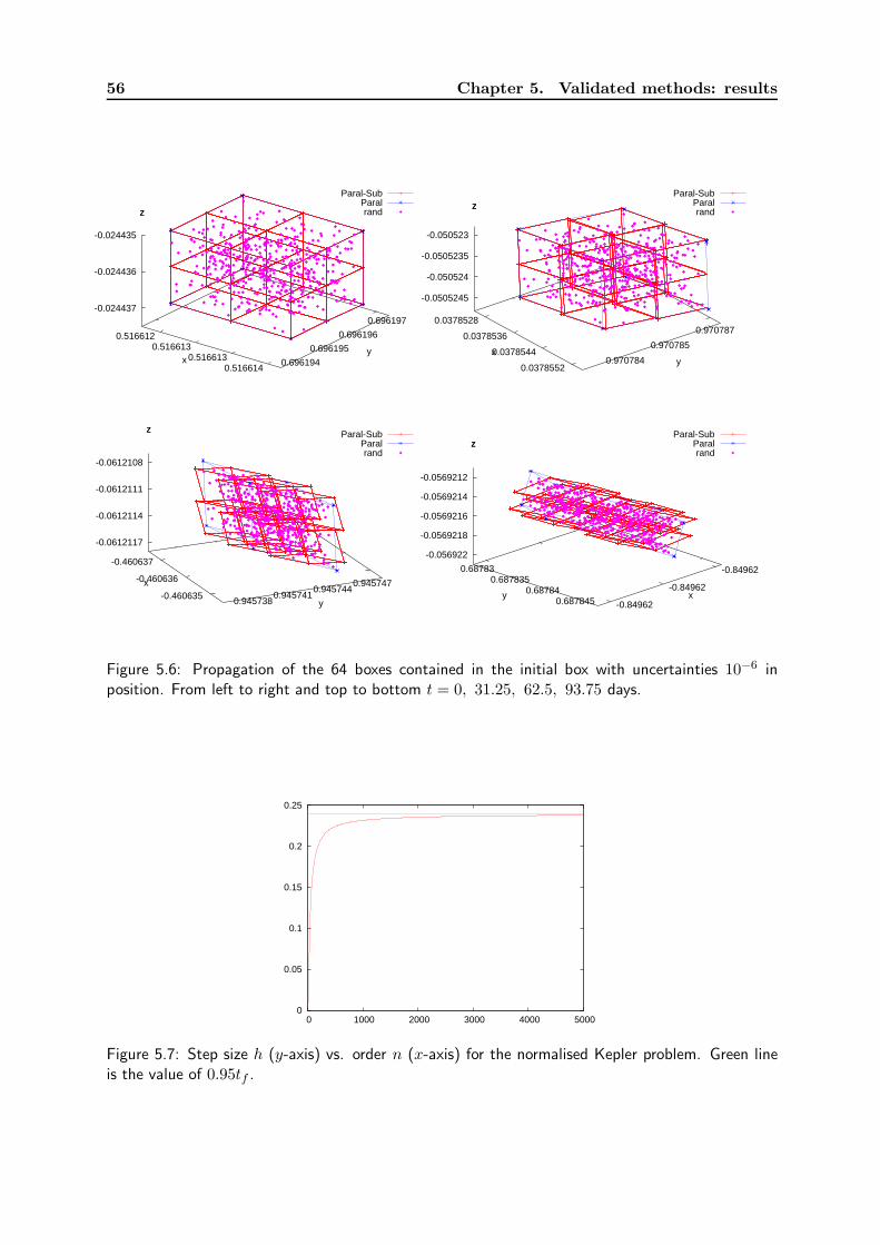
56 Chapter 5. Validated methods: results
0.516612 0.516613
0.516613 0.516614
0.696194
0.696195
0.696196
0.696197-0.024437
-0.024436
-0.024435
z
Paral-SubParalrand
xy
z
0.0378528
0.0378536
0.0378544
0.0378552 0.970784
0.970785
0.970787
-0.0505245
-0.050524
-0.0505235
-0.050523
zParal-Sub
Paralrand
xy
z
-0.460637
-0.460636
-0.460635 0.945738 0.945741
0.945744 0.945747
-0.0612117
-0.0612114
-0.0612111
-0.0612108
z Paral-SubParalrand
x
y
z
-0.84962
-0.84962
-0.84962
0.68783 0.687835
0.68784 0.687845
-0.056922
-0.0569218
-0.0569216
-0.0569214
-0.0569212
zParal-Sub
Paralrand
xy
z
Figure 5.6: Propagation of the 64 boxes contained in the initial box with uncertainties 10−6 inposition. From left to right and top to bottom t = 0, 31.25, 62.5, 93.75 days.
0
0.05
0.1
0.15
0.2
0.25
0 1000 2000 3000 4000 5000
Figure 5.7: Step size h (y-axis) vs. order n (x-axis) for the normalised Kepler problem. Green lineis the value of 0.95tf .

5.4. Validated integration of the low-thrust problem 57
1
2
3
4
5
6
7
0 10 20 30 40 50 60 70
Figure 5.8: Evolution of the step size along the integration, for the alternative method proposed inSection 5.2. Step size h in days (y-axis) vs. iterate of validated integration (x-axis) for the ApophisKepler problem.
-0.003-0.002
-0.001 0
0.001-0.002-0.001
0 0.001
0.002
-0.002
-0.001
0
0.001
z
I order QRI order Paral
Earth
x
y
z
Figure 5.9: In red, the part of trajectory integrated with a first order QR–Lohner method, about 43days. In blue, with a first order parallelepiped one, about 9 days. In black, the Earth. The initial boxconsidered is the one centred at the point given in Tables 3.10 and 3.11 and setting an uncertaintyin space of 10−12 AU and null uncertainty for the thrust. Unit AU.

58 Chapter 5. Validated methods: results
5.5 Summary
Here we summarise the results obtained in this chapter. We have developed three differentinterval based methods:
• Parallelepiped,
• QR - Lohner,
• KT - equivariant.
First, we have tested them for the Kepler problem using a first and second order approach,following the ideas of the original Moore’s algorithm. In Table 5.12 we can see these results forall these methods taking an initial uncertainty of ±10−6 and an integration step size h = 0.625.
Parallelepiped QR - Lohner KT - equivariant
1st order 268.75 493.75 473.75
2nd order 893.75 681.25 481.25
Table 5.12: Comparison of the maximum time of integration (in days) obtained for the 3 differentmethods using 1st and 2nd order approaches. In all the computations we have taken a step sizeh = 0.625 days and an initial uncertainty of ±10−6
As the step size provided by the classical rough enclosure method is very small, we have de-veloped a new strategy (see Section 5.2), adapted for the Kepler problem, that can be generalizedto N -body problems). This allows to use step sizes about 7 times larger (see Figure 5.8).
We have also developed and tested three different subdivision strategies (see Section 5.1.2for more details on the differences) and we have tested them using the parallelepiped method.In Table 5.13 we can see the results of applying the different subdivision strategies with the firstand second order methods. In Table 5.6 we can see the results of considering the two subdivisionstrategies and applying them for a different number of subdivisions.
1st order 2nd order Subdiv 1 Subdiv 2i Subdiv 2ii
268.75 893.75 340 313 441.25
Table 5.13: Comparison of the maximum time of integration (in days) obtained for the parallelepipedmethod using 1st and 2nd order approaches and different subdivision strategies. In all the computa-tions a step size h = 0.625 days and an initial uncertainty of ±10−6 is used.
According to the previous results and the accuracy of the computed interval boxes it seemsthat the parallelepiped method is the best choice. We have applied this method, using thefirst and second order approaches, to our two applications: the motion of a NEO, taking theparticular case of Apophis, and the motion of a low-thrust probe in the Earth-Moon system.
Table 5.7 shows the results for the Apophis case, taking and integration step size h = 0.0625.We can see that, in this case, taking the second order parallelepiped method is much better. Wenotice that the results are very similar to the results obtained for the Kepler problem.
In Tables 5.8, 5.9, 5.10 and 5.11 we can see the results for the motion of a low-thrust probe.In this case we can see that the gain obtained when we consider second order methods is almostnegligible.

59
Chapter 6
Conclusions and future work
6.1 Conclusions
After looking at the topics presented in this report and to the available literature on Self Vali-dated Integrators, the following conclusions have been reached:
1) For non-validated integrations, the Taylor method has been widely tested. In the case ofnon-stiff equations, for analytic vector fields or, at least, for sufficiently regular ones, itseems to be a good choice.
Main points are: 1. Recurrent computation of higher order coefficients by automaticdifferentiation; 2. Truncation error negligible in front of round off errors; 3. Suitable orderfor optimal performance, and 4. Optimal step size depending only of the local radius ofconvergence of the expansion and, in particular, independent of the number of digits usedin the computations.
The propagation of the round off errors in the first integrals displays the characteristicsof a random walk. In some sense, one cannot do better. Furthermore, for given initialconditions and final time one easily obtains that the cost is proportional to d4 when workingwith an arithmetic with d digits.
It also allows to implement the integration of variational equations. This, in turn, gives away to propagate a box of initial data.
2) When dealing with intervals the key problems to face are dependency and wrapping. Theirinfluence in the integration of ODE is crucial, specially for relatively long time intervals.
It is important to note that we can consider two different kinds of problems. First oneappears if our purpose is to give a Computer Assisted Proof of some fact like existenceof a periodic solution or a transversal homoclinic solution. Second one concerns with thepropagation of a given initial set of data.
In the first case it is possible to use a large number of digits. This allows to “delay” theapparition of problems due to dependency and wrapping. A good and efficient implemen-tation of interval arithmetic is essential to speed up the computations.
In the second case, if the initial box is relatively large, then the proper dynamics canlargely increase the size of the box. This occurs, typically, at a linear rate, for integrableHamiltonian systems, like Kepler’s problem. The behaviour is similar for an asteroid,except during the periods of close approaches. Then, as in the general case of chaoticsystems, the rate of increase is exponential.
In this last case the influence of the errors introduced by the arithmetic is almost negligible.The bad problem is that all estimates must be done in large boxes. As mentioned at the

60 Chapter 6. Conclusions and future work
end of Section 5.1.1, even in a simple model describing the rate of increase of the size ofthe boxes, the procedures lead to a singularity in the size of the boxes.
3) Our efforts have been devoted to the implementation of algorithms based of Lohner algo-rithm and variants. We have found three, non independent, main sources of difficulties.We describe them shortly and how we have tried to solve them.
a) First one concerns with rough enclosure. Starting with a current box at some momentt∗ of the integration one should find another box which contains the image of thatbox for all t in the interval [t∗, t∗ + h], where h is the current time step. This is doneto obtain existence of the solution and to bound the errors of the Taylor method usedto do one time step. The procedure is iterative and the value of h has to be verysmall, of the order of the inverse of the Lipschitz constant of the vector field, to haveconvergence. This constant can increase in a non-admissible way when the size of theboxes increase far beyond the true size of the propagation of the starting box, due todependency and wrapping.
The fact that the rough enclosure is small is not critical concerning the final re-sult about the size of the boxes at a given final time, but it affects, definitely, thecomputing time.
An approach which largely improves the computations skips the computation of roughenclosure and replaces it by analytical estimates, based on the domain of analyticityof the vector field. Using tools from analysis we have been able to produce lower esti-mates of the radius of convergence and upper estimates of the remainder. AppendixB contains a sketch of the method for Kepler’s problem. It can be extended to theperturbations of other bodies and to general analytic vector fields.
b) Next difficulty is dependency. At every operation one takes the worst case among allthe possible choices of elements contained in the boxes involved in the operation. But,in general, they are not independent because they can come from different real numbercomputations done with the same elements. To compute f(I) for all elements x in aset I is an almost impossible task if the computation of f involves many individualoperations and we want to produce sharp estimates.
A mild remedy we have tried is to change the interval arithmetic in the elementarycase of computing squares of real intervals. But the improvement is minor. A betterapproach is based on subdivision, to be commented in next item.
c) Last problem is wrapping. Every time an operation with sets is done, we must putthe result inside a set of a given class, using some suitable representation. To mimicthe behaviour of the true dynamics a convenient method consists in representing thesets as a central point plus a matrix applied to a product of intervals in R. This ishow boxes propagate under the first variational equations. The size of the boxes hasto be increased to account for the remainder and errors in the operations.
An important difficulty is that the differential matrix, even keeping the symplecticcharacter in the integration of Hamiltonian systems, can have a strong increase inthe condition number. Some representations like QR or similar decompositions canimprove the results in a moderate way.
In the case of Kepler problem (integrated without taking into account any specialproperty, like passing to action angle variables) both dependency and wrapping pro-duce an increase of the size of the box across the orbit. This implies changes in theenergy, hence in the frequency and, therefore, in the size along the orbit.
A suitable method to cope with these difficulties is subdivision. This can be done attwo different places:
6.1. Conclusions 61
A. On the initial box of data.
B. When an initial box is propagated under the algorithm, instead of putting theimage of the box inside a product of intervals, it can be covered by small boxes ofthe same kind, with a minimal covering.
Anyway, subdivision has the drawback of a strong increase in the computing time.This is specially dramatic when the dimension of the phase space is high. Dimension 6gives not so many chances to subdivide in small elements with a reasonable computingtime.
4) As a result of the experiments carried out inside this project we conclude that Lohner-likebase methods are suitable when the following conditions are satisfied:
A. The size of the initial set of data is very small.
B. The time interval during which the system has to be integrated is moderate.
C. The rate of increase of the size of the boxes is moderate.
Even if these condition hold, it is quite convenient to try to avoid the computation of roughenclosures and replace them by analytical estimates. This can decrease in a significativeway the computing time.
5) Another possibility, yet to be explored, is the use of Taylor based methods, not only forthe time integration but also for the propagation of an initial set of points. That is,at every time step one should produce a Taylor expansion with respect to the variationof the initial conditions plus a (hopefully) small box containing the propagated effect ofremainders (in the time step and in the phase space variables) plus the effect of the errorsin the operations.
From a mathematical point of view what is done is a propagation of the solution as atruncated jet (a polynomial) representation in terms of the initial conditions, with controlon all errors.
This method allows to decrease most of the problems due to dependency and wrapping.The price to be payed is the computational cost. In some sense it can be consideredas a Lohner-like method of high order in which boxes are kept to a minimal size. Theimplementation also differ. While Ck Lohner methods integrate variational equations, thepropagation of the jet in Taylor based methods is done symbolically, using routines for allthe required operations as polynomials in several variables.
Anyway, even these methods require subdivision when the size of the propagated box istoo large and the intervals bounding the remainder exceed a given size.
6) An important point is the optimality of the algorithms used, not only considering sharpnessof the results, but also computing time. Preliminary attempts are included in AppendicesA and B.
The fact that both time integration and dependence with respect to initial conditions areobtained by Taylor methods (or, equivalently, integration of variational equations) raisesthe problem of optimal orders with respect to each one of the variables, both time step andphase space variables. If the sizes of an initial box are quite different in different directionsthe orders of the expansion must adapt to that fact.
Careful a priori operation counts, which strongly depend on the algorithms used, allow todiscuss the optimal strategy concerning subdivision. This also gives the optimal step sizeto be used to achieve optimal performance keeping an admissible bound on errors.

62 Chapter 6. Conclusions and future work
6.2 Future work
The study of the literature on the topic, the experience gained in this project, the difficultiesencountered during its realisation and the analysis we have done of the problem suggest severallines of future work. We consider that they are quite promising.
i) Definitely gain also experience by implementing Taylor based methods. The dependenceand wrapping effects seem to influence too strongly Lohner-like algorithms for the transportof big boxes during long time intervals.
ii) Items 4) and 5) in the Conclusions give a first indication about when it is suitable to useone of the two main approaches to deal with a given problem. After i) above, explicitcomparisons of the relative performance should be done in a battery of problems.
iii) Analytical methods to obtain estimates for radius of convergence in the time integration,in bounding the remainder and in the domain of validity and remainder in the phasespace variables should provide an alternative to other estimates. This requires location ofsingularities of the vector field in the complex phase space, Cauchy estimates for boundof the rates of increase of the coefficients in a polydisc, etc. Even for entire vector fields(e.g., a polynomial vectorfield) the solutions display generically singularities, perhaps forsome complex time, which give the local radius of convergence.
iv) A delicate point is the optimality of the expansions used concerning efficiency. The vectorfield can be the sum of different contributions, like in the asteroid case. The main effectis the solar attraction and the effect of the other bodies is a perturbation, except in closeapproaches to a planet or moon, where the roles exchange.
Taylor series for time integration can be computed to a different order for each one of thecontributions, taking into account, of course, the couplings between the different terms(the so-called indirect effects in Celestial Mechanics). Optimality can then require s subtlestrategy. We consider worth to explore this.
A similar thing appears with the suitable orders to be used in the expansions in the phasespace variables, with respect to each one of the variables.
v) Final topic of future work can be the inclusion of random terms in the vector field, suchas uncertainties in some forces, errors in the execution of manoeuvres, etc. This is easilydone in Lohner-like algorithms, while it requires the inclusion of additional variables inTaylor based methods.
Uncertainties and errors in manoeuvres, as mentioned, have typically a statistical distri-bution, according to a given probability law. In the case of compact support this can beapproximated by a distribution of probabilities in a finite set of small boxes. This is alsotrue, for instance, in the propagation of a set of initial conditions for an asteroid, whereorbit determination provides a statistical distribution of errors.
Rigorous methods should be able to deliver a (discrete) approximation of the propagateddistribution of probability. This is really important but still seems to be far in the futureand will require a strong use of parallelism. But one should keep the point in mind.
6.3 Acknowledgements
We thank Gerard Gomez, Tomasz Kapela, Marıa Eugenia Sansaturio, Daniel Wilczak and PiotrZgliczynski for technical help. Computer facilities were provided by the Spanish Ministery ofEducation and Generalitat de Catalunya.

Bibliography 63
Bibliography
[AH83] G. Alefeld and J. Herzberger. Introduction to interval computations. Com-puter Science and Applied Mathematics. Academic Press Inc. [Harcourt BraceJovanovich Publishers], New York, 1983. Translated from the German by JonRokne.
[BBCG96] M. Berz, C. Bischof, G.F. Corliss, and A. Griewank, editors. ComputationalDifferentiation: Techniques, Applications, and Tools. SIAM, Philadelphia, Penn.,1996.
[BCCG92] C.H. Bischof, A. Carle, G.F. Corliss, and A. Griewank. ADIFOR: Automaticdifferentiation in a source translation environment. In Paul S. Wang, editor, Pro-ceedings of the International Symposium on Symbolic and Algebraic Computation,pages 294–302, New York, 1992. ACM Press.
[BKSF59] L.M. Beda, L.N. Korolev, N.V. Sukkikh, and T.S. Frolova. Programs for au-tomatic differentiation for the machine BESM. Technical Report, Institute forPrecise Mechanics and Computation Techniques, Academy of Science, Moscow,USSR, 1959. (In Russian).
[BMH01] M. Berz, K. Makino, and J. Hoefkens. Verified integration of dynamics in thesolar system. Nonlinear Anal., 47(1):179–190, 2001.
[Bro71] R. Broucke. Solution of the N -Body Problem with recurrent power series. Ce-lestial Mech., 4(1):110–115, 1971.
[BWZ70] D. Barton, I.M. Willers, and R.V.M. Zahar. The automatic solution of ordinarydifferential equations by the method of Taylor series. Computer J., 14(3):243–248,1970.
[CC82] G.F. Corliss and Y.F. Chang. Solving ordinary differential equations using Taylorseries. ACM Trans. Math. Software, 8(2):114–144, 1982.
[CC94] Y.F. Chang and G.F. Corliss. ATOMFT: Solving ODEs and DAEs using Taylorseries. Computers and Mathematics with Applications, 28:209–233, 1994.
[Cor95] G.F. Corliss. Guaranteed error bounds for ordinary differential equations. InM. Ainsworth, J. Levesley, W. A. Light, and M. Marletta, editors, Theory ofNumerics in Ordinary and Partial Differential Equations, pages 1–75. OxfordUniversity Press, Oxford, 1995. Lecture notes for a sequence of five lectures atthe VI-th SERC Numerical Analysis Summer School, Leicester University, 25 -29 July, 1994.
[Dan88] J.M.A. Danby. Fundamentals of celestial mechanics. Richmond, Va., U.S.A.:Willmann-Bell, 1988.2nd ed., enl., 1988.

64 Bibliography
[EKW84] J.-P. Eckmann, H. Koch, and P. Wittwer. A computer-assisted proof of univer-sality for area-preserving maps. Mem. Amer. Math. Soc., 47(289):vi+122, 1984.
[GBO+08] J.D. Giorgini, L.A.M. Benner, S.J. Ostro, M.C. Nolan, and M.W. Busch. Pre-dicting the Earth encounters of (99942) Apophis. Icarus, 193:1–19, 2008.
[GC91] A. Griewank and G.F. Corliss, editors. Automatic Differentiation of Algorithms:Theory, Implementation, and Application. SIAM, Philadelphia, Penn., 1991.
[Gib60] A. Gibbons. A program for the automatic integration of differential equationsusing the method of Taylor series. Comp. J., 3:108–111, 1960.
[Gol91] A. Goldberg. What every computer scientist should know about floating-pointarithmetic. ACM Computing Surveys, 23(1):5–48, 1991.
[Gri00] A. Griewank. Evaluating Derivatives. SIAM, Philadelphia, Penn., 2000.
[HB03] J. Hoefkens and M. Berz. Controlling the wrapping effect in the solution of ODEsfor asteroids. Reliab. Comput., 9(1):21–41, 2003.
[Hoe01] J. Hoefkens. Rigorous numerical analysis with high order Taylor methods. PhDthesis, Michigan State University, 2001.
[IS90] D.H. Irvine and M.A. Savageau. Efficient solution of nonlinear ordinary differ-ential equations expressed in S-system canonical form. SIAM J. Numer. Anal.,27(3):704–735, 1990.
[JPL] http://ssd.jpl.nasa.gov/horizons.html.
[JV97] A. Jorba and J. Villanueva. On the persistence of lower dimensional invarianttori under quasi-periodic perturbations. J. Nonlinear Sci., 7:427–473, 1997.
[JZ05] A. Jorba and M. Zou. A software package for the numerical integration of ODEsby means of high-order Taylor methods. Exp. Math., 14(1):99–117, 2005.
[KS07] T. Kapela and C. Simo. Computer assisted proofs for nonsymmetric planarchoreographies and for stability of the Eight. Nonlinearity, 20(5):1241–1255,2007.
[Lan82] Oscar E. Lanford, III. A computer-assisted proof of the Feigenbaum conjectures.Bull. Amer. Math. Soc. (N.S.), 6(3):427–434, 1982.
[Loh] Lohner. http://www.math.uni-wuppertal.de/ xsc/xsc/pxsc software.html#awa.
[LTWVG+06] M. Lerch, G. Tischler, J. Wolff Von Gudenberg, W. Hofschuster, and W. Kramer.FILIB++, a fast interval library supporting containment computations. ACMTrans. Math. Software, 32(2):299–324, 2006.
[Mak98] K. Makino. Rigorous analysis of nonlinear motion in particle accelerators. PhDthesis, Michigan State University, 1998.
[MB05] K. Makino and M. Berz. Suppression of the wrapping effect by Taylor model-based verified integrators: long-term stabilization by preconditioning. Int. J.Differ. Equ. Appl., 10(4):353–384 (2006), 2005.

Bibliography 65
[MCS+05] A. Milani, S.R. Chesley, M.E. Sansaturio, G. Tommei, and G.B. Valsecchi. Non-linear impact monitoring: line of variation searches for impactors. Icarus, 173:362– 384, 2005.
[MH92] K.R. Meyer and G.R. Hall. Introduction to Hamiltonian Dynamical Systems andthe N-Body Problem. Springer, New York, 1992.
[Moo66] R.E. Moore. Interval Analysis. Prentice-Hall, Englewood Cliffs, N.J., 1966.
[Moo79] R.E. Moore. Methods and applications of interval analysis, volume 2 of SIAMStudies in Applied Mathematics. Society for Industrial and Applied Mathematics(SIAM), Philadelphia, Pa., 1979.
[Mou14] F.R. Moulton. An introduction to celestial mechanics. New York, The Macmillancompany; [etc., etc.] 1914. 2d rev. ed., 1914.
[MZ00] M. Mrozek and P. Zgliczynski. Set arithmetic and the enclosing problem indynamics. Ann. Polon. Math., 74:237–259, 2000. Dedicated to the memory ofBogdan Ziemian.
[Ned99] N.S. Nedialkov. Computing rigorous bounds on the solution of an initial valueproblem for an ordinary differential equation. PhD thesis, University of Toronto,1999.
[NEO] http://unicorn.eis.uva.es/cgi-bin/neodys/neoibo?objects:Apophis.
[NJ01] N.S. Nedialkov and K.R. Jackson. A new perspective on the wrapping effect ininterval methods for initial value problems for ordinary differential equations. InPerspectives on enclosure methods (Karlsruhe, 2000), pages 219–264. Springer,Vienna, 2001.
[NJC99] N.S. Nedialkov, K.R. Jackson, and G.F. Corliss. Validated solutions of ini-tial value problems for ordinary differential equations. Appl. Math. Comput.,105(1):21–68, 1999.
[NJN07] M. Neher, K.R. Jackson, and N.S. Nedialkov. On Taylor model based integrationof ODEs. SIAM J. Numer. Anal., 45(1):236–262 (electronic), 2007.
[Pol76] H. Pollard. Celestial mechanics. Mathematical Association of America, Wash-ington, D. C., 1976. Carus Mathematical Monographs, No. 18.
[Ral81] L.B. Rall. Automatic Differentiation: Techniques and Applications, volume 120of Lecture Notes in Computer Science. Springer Verlag, Berlin, 1981.
[Ron05] R.B. Roncoli. Lunar constants and models document. JPL Technical DocumentD-32296, 2005.
[Sei92] P. K. Seidelmann. Explanatory Supplement to the Astronomical Almanac. Pub-lished by University Science Books, 648 Broadway, Suite 902, New York, NY10012, 1992. Completely revised and rewritten, edited by Seidelmann, P. Ken-neth, 1992.
[Sim01] C. Simo. Global dynamics and fast indicators. In H.W. Broer, B. Krauskopf, andG. Vegter, editors, Global analysis of dynamical systems, pages 373–389, Bristol,2001. IOP Publishing.

66 Bibliography
[SMA] SMART-1. http://smart.esa.int/science-e/www/area/index.cfm?fareaid=10.
[SS71] E. L. Stiefel and G. Scheifele. Linear and regular celestial mechanics. Perturbedtwo-body motion, numerical methods, canonical theory. Springer-Verlag, NewYork, 1971.
[Ste56] J.F. Steffensen. On the restricted problem of three bodies. Danske Vid. Selsk.Mat.-Fys. Medd., 30(18):17, 1956.
[Ste57] J.F. Steffensen. On the problem of three bodies in the plane. Mat.-Fys. Medd.Danske Vid. Selsk., 31(3):18, 1957.
[SV87] M.A. Savageau and E.O. Voit. Recasting nonlinear differential equations as S-systems: a canonical nonlinear form. Math. Biosci., 87(1):83–115, 1987.
[SW] M.E. Standish and J.G. Williams. Detailed description of the JPL planetaryand lunar ephemerides, DE405/LE405. Electronically available as a PDF file,http://iau-comm4.jpl.nasa.gov/XSChap8.pdf.
[Wen64] R. E. Wengert. A simple automatic derivative evaluation program. Comm. ACM,7(8):463–464, 1964.
[WZ08] D. Wilczak and P. Zgliczynski. Cr-lohner algorithm. arXiv:0704.0720v1, 2008.
[Zgl02] P. Zgliczynski. C1 Lohner algorithm. Found. Comput. Math., 2(4):429–465, 2002.
[Zgl07] P. Zgliczynski. Advanced course on Computer Assisted Proofs in Dynamics,University of Barcelona, 2007. The notes of the course can be retrieved fromhttp://www.imub.ub.es/cap07/slides/.

67
Appendix A
N-body variationals, asteroid case
A.1 Set up and variational equations
We want to integrate the variational equations for an asteroid, at the same time that the motion,correcting the position of the N main bodies by using the JPL 405 ephemerides (or not).
The equations of motion for the asteroid can be written as
xA = fx =
N∑
j=1
mj(xj − xA)r−3j,A, r2j,A = (xj − xA)2 + (yj − yA)2 + (zj − zA)2,
and similar equations for the other coordinates: yA = fy, zA = fz.
Let ξ, η, ζ denote the first three components of the solution of the first order variationalequations, written in vector form. It is clear that it is enough to obtain the Taylor solutions ofthese. Then, the first derivatives with respect to time, easily computable from the jets of ξ, η, ζ,give the remaining 3 components, and starting with the different columns of the identity matrixwe recover the full first variational matrix.
Note that the effect of the changes of velocities appears due to the fact that the velocitiesgive the terms of order 1 in the jet of the coordinates. This means that, instead of 6×6 equationswe need only to integrate 3 × 6.
To this end we write
ξ = Dxfxξ +Dyfxη +Dzfxζ, η = Dxfyξ +Dyfyη +Dzfyζ, ζ = Dxfzξ +Dyfzη +Dzfzζ,
which gives the recurrences to be used in Taylor’s method. ObviouslyDxfx denotes the derivativeof fx w.r.t. xA and similar for the others. As the 3 × 3 matrix containing the D∗f∗ is minusthe Hessian of the Hamiltonian w.r.t. the position coordinates of the asteroid, it is symmetric:Dxfy = Dyfx, etc.
A trivial computation gives
Dxfx =
N∑
j=1
mj
(
−r−3j,A + 3(xj − xA)2r−5
j,A
)
, Dyfx =
N∑
j=1
mj3(xj − xA)(yj − yA)r−5j,A,
and similar for the other cases.
To obtain the second (and higher) order variational equations it is better to use indices. Letw = (w1, w2, w3)
T = (x, y, z)T and denote as w0 the initial values. The values w4, w5, w6 denotethe respective time derivatives. As mentioned these velocities appear as initial conditions (i.e.,in w0) but in w only the position coordinates are necessary. We shall use the shorter notation

68 Appendix A. N-body variationals, asteroid case
wn,i, wm,ij , wm,ijk, etc to denote∂wn
∂w0i
,∂2wn
∂w0i ∂w
0j
,∂3wn
∂w0i ∂w
0j∂w
0k
, etc. From the first variational
equations
d2
dt2∂wm
∂w0i
=
3∑
k=1
∂fwm
∂wk
∂wk
∂w0i
, ord2
dt2wm,i =
3∑
k=1
∂fwm
∂wkwk,i,
we obtain immediately
d2
dt2wm,ij =
3∑
n,p=1
∂2fwm
∂wn∂wpwn,iwp,j +
3∑
n=1
∂fwm
∂wnwn,ij .
Recall that the initial conditions are wm,ij = 0 and the same happens for the initial conditions ofhigher order variational equations. These solutions differ because the equations contain wn,iwp,j
or similar terms, which do depend on the initial changes in both positions and velocities. Alsothe symmetry w.r.t. the indices i, j allows to reduce dimension. Instead of 36 different sets ofinitial conditions for the initial variations of the positions and velocities w0
i , w0j , it is enough to
use 21. This has to be done for each one of the 3 variables wm. These considerations reduce the
total number of second order variationals from 216 to 63, that is 3 ×(
75
)
.
The equations involve second derivatives∂2fwm
∂wk∂wn, which can be computed as
∂2fx
∂x2=
N∑
j=1
mj
(
−9(xj − xA)r−5j,A + 15(xj − xA)3r−7
j,A
)
,
∂2fx
∂x∂y=
N∑
j=1
mj
(
−3(yj − yA)r−5j,A + 15(xj − xA)2(yj − yA)r−7
j,A
)
,
∂2fx
∂y∂z=
N∑
j=1
mj15(xj − xA)(yj − yA)(zj − zA)r−7j,A,
the remaining ones being obtained from the symmetries or by cyclic permutation of indices.These formulas can be computed in different ways, to minimise the number of operations, asshall be discussed later.
If we go to third and fourth order variationals (we shall refrain to go farther explicitly) theequations become
d2
dt2wm,ijk =
3∑
n,p,q=1
∂3fwm
∂wn∂wp∂wqwn,iwp,jwq,k+
3∑
n,p=1
∂2fwm
∂wn∂wp(wn,ijwp,k +wn,ikwp,j + wn,jkwp,i) +
3∑
n=1
∂fwm
∂wnwn,ijk ,
d2
dt2wm,ijkl =
3∑
n,p,q,r=1
∂4fwm
∂wn∂wp∂wq∂wrwn,iwp,jwq,kwr,l +
3∑
n,p,q=1
∂3fwm
∂wn∂wp∂wq×
(wn,ijwp,kwq,l+wn,ikwp,jwq,l+wn,ilwp,jwq,k+wn,jkwp,iwq,l+wn,jlwp,iwq,k+wn,klwp,iwq,j) +
3∑
n,p=1
∂2fwm
∂wn∂wp(wn,ijwp,kl + wn,ikwp,jl + wn,jkwp,il +wn,ijkwp,l) +
3∑
n=1
∂fwm
∂wnwn,ijkl .

A.2. A count on operations 69
Furthermore the number of equations to be integrated, taking into account the symme-
tries, for the variational equations of order s is 3 ×(
s+ 55
)
. For orders 3, 4, 5, . . . we obtain
168, 378, 756, . . ., respectively.
It has to be stressed that, while in the second and third variational equations a factor
which comes from a derivative of fwm, like∂2fwm
∂wn∂wp, multiplies products of the solutions of the
previous variationals equations of the same type, like wn,ijwp,k in the third order variational, forvariationals of order greater than 3 this is not true in general. For instance, in the fourth order
variationals∂2fwm
∂wn∂wpmultiplies both terms of the forms wn,ijwp,kl and wn,ijkwp,l. This comes
from the fact that, in general, in the partitions of a number there exist several partitions in thesame number of pieces. In the example 4 = 2 + 2 = 3 + 1.
A.2 A count on operations
Let us start a count on operations. Assuming that we work up to order M in the Taylor seriesand that the order is kept fixed for all the computed variationals, we assume that the cost of aproduct, a square and a power are, respectively,
M2,1
2M2 and 2M2.
A first part of the cost comes from the integration of the motion of the N massive bodies.Even if we use JPL ephemerides, the jet for the asteroid depends on the jets of the N bodies. Forevery term in the sums we have to compute: ∆xi,j = xj−xi, ∆yi,j = yj−yi, ∆zi,j = zj−zi,∆x2
i,j,
∆y2i,j, ∆z2
i,j , that is, 3 squares. Then we have immediately r2i,j and it remains to compute a
power (r2i,j)−3/2 and then its products by ∆xi,j, ∆yi,j, ∆zi,j, etc. In all we have an estimate
(
N2
)
× (3 × 1
2+ 2 + 3) ×M2 =
13
2M2
(
N2
)
.
Next step is the computation of the jet of the asteroid. Instead of following the above method,we compute in a slightly different order which is a little bit better when including variationals.For each one of the N bodies we compute the contributions as:
∆xj,A, ∆yj,A, ∆zj,A, ∆x2j,A, ∆y2
j,A, ∆z2j,A, r
2j,A, 1/rj,A, 1/r2j,A,
∆xj,A/r2j,A, ∆yj,A/r
2j,A,∆j,A/r
2j,A, ∆xj,A/r
3j,A, ∆yj,A/r
3j,A, ∆j,A/r
3j,A.
In all, 4 squares, 1 power and 6 products, with a cost 10NM2.
Then the successive derivatives,∂fwm
∂wn,∂2fwm
∂wn∂wp,
∂3fwm
∂wn∂wp∂wqare computed, recurrently, by
multiplication of jets already available by the jet of one of the expressions 1/r2j,A, ∆xj,A/r2j,A,
∆yj,A/r2j,A, ∆j,A/r
2j,A. The cost for the derivatives of increasing order of f which appear in
the first, second, third, fourth, fifth, ... order variationals is, in multiples of NM2, equal to1 + 6 = 7, 3 + 10 = 13, 1 + 6 + 15 = 22, 3 + 10 + 21 = 34, 1 + 6 + 15 + 28 = 50, etc. It willbe clear in a moment that this cost becomes negligible, for a fixed N , when the order of thevariationals increases.
The computation of the right hand sides of the variationals requires several steps:
1) Computing the derivatives of fwm, already discussed in last paragraph.
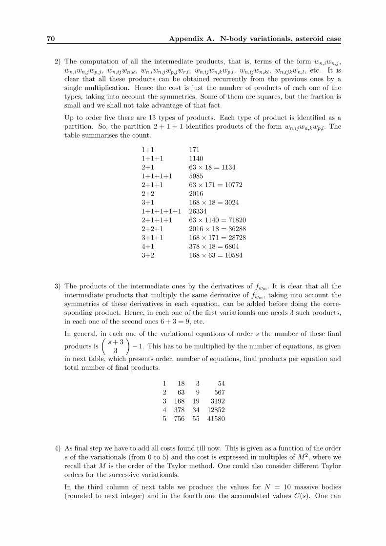
70 Appendix A. N-body variationals, asteroid case
2) The computation of all the intermediate products, that is, terms of the form wn,iwn,j,wn,iwn,jwp,j, wn,ijwn,k, wn,iwn,jwp,jwr,l, wn,ijwn,kwp,l, wn,ijwn,kl, wn,ijkwn,l, etc. It isclear that all these products can be obtained recurrently from the previous ones by asingle multiplication. Hence the cost is just the number of products of each one of thetypes, taking into account the symmetries. Some of them are squares, but the fraction issmall and we shall not take advantage of that fact.
Up to order five there are 13 types of products. Each type of product is identified as apartition. So, the partition 2 + 1 + 1 identifies products of the form wn,ijwn,kwp,l. Thetable summarises the count.
1+1 1711+1+1 11402+1 63 × 18 = 11341+1+1+1 59852+1+1 63 × 171 = 107722+2 20163+1 168 × 18 = 30241+1+1+1+1 263342+1+1+1 63 × 1140 = 718202+2+1 2016 × 18 = 362883+1+1 168 × 171 = 287284+1 378 × 18 = 68043+2 168 × 63 = 10584
3) The products of the intermediate ones by the derivatives of fwm. It is clear that all theintermediate products that multiply the same derivative of fwm, taking into account thesymmetries of these derivatives in each equation, can be added before doing the corre-sponding product. Hence, in each one of the first variationals one needs 3 such products,in each one of the second ones 6 + 3 = 9, etc.
In general, in each one of the variational equations of order s the number of these final
products is
(
s+ 33
)
− 1. This has to be multiplied by the number of equations, as given
in next table, which presents order, number of equations, final products per equation andtotal number of final products.
1 18 3 542 63 9 5673 168 19 31924 378 34 128525 756 55 41580
4) As final step we have to add all costs found till now. This is given as a function of the orders of the variationals (from 0 to 5) and the cost is expressed in multiples of M2, where werecall that M is the order of the Taylor method. One could also consider different Taylororders for the successive variationals.
In the third column of next table we produce the values for N = 10 massive bodies(rounded to next integer) and in the fourth one the accumulated values C(s). One can

A.3. On the optimal variational order to propagate a box 71
check that the role of N is negligible for s > 2. Furthermore, for s > 3 most of the costcomes from the computation of the intermediate products.
0 13N(N − 1)/4 + 10N 393 3931 7N + 54 124 5172 13N + 738 868 13753 22N + 5466 5686 70614 34N + 34650 34990 420515 50N + 222138 222638 264689
A fit of the accumulate results shows that the rate of increase for s > 1 behaves roughly likeC(s) = c1 exp(c2s), but that value of c2 increases slowly when only the last 3 or 2 points aretaken. A working value of c2 can be 1.85.
A.3 On the optimal variational order to propagate a box
Now we face the problem of the optimality of the order of the variationals when we want topropagate a given box. We start with a suitable set up and assumptions:
a) We start at some time t0 = 0 and want to arrive at a time tf . The goal is to transporta box with sides of typical size ℓ. The analysis can be easily modified if not all of thesides are equal. There is freedom in the selection of the order of the variationals used totransport boxes.
b) We assume that the error in the representation of the map time-tf using up to order s inthe variationals, is of the type Kf (ℓ/Rf )s+1, where Rf is the radius of convergence andKf the factor in the Cauchy estimates. One desires a bound of the error of the form
Kf (ℓ/Rf )s+1 ≤ ε,
for some fixed value of ε.
c) Independently of the dimension of the problem we assume that the problem has mainlyd unstable directions, either because of positive Lyapunov exponents or because there isa strong shear in one or more directions. For instance, in Kepler’s problem or mildlyperturbed Kepler’s problems one has d = 1 because of the shear along the orbit.
d) To achieve the goal it is possible to subdivide the box of size ℓ in boxes of size ℓ/m in eachone of the d directions. Of course, the values of m can be different in each direction, butwe shall take them equal for simplicity. An increase of the order of the variationals allowsto take less subboxes, at the price of a higher cost. We want to optimise.
e) We also assume that the number of steps Sf is independent of the order of the variationalsused. Furthermore, for simplicity, we assume the subdivision is done at t0. Other strategiesare possible, using different subdivisions at different stages of the integration.
Then the value of m is selected as m =ℓ
Rf
(
ε
Kf
)−1/(s+1)
and the total cost is
SfC(s)
[
ℓ
Rf
(
ε
Kf
)−1/(s+1)]d
.

72 Appendix A. N-body variationals, asteroid case
We assume C(s) = c1 exp(c2s), introduce ε = ε/Kf and take logarithms. Skipping all terms notdepending on s, we obtain
c2s+d
s+ 1log(ε−1),
for which the minimum is attained for s+ 1 =√
d log(ε−1)/c2.
A rough application to the asteroid problem assuming d = 1, c2 = 1.85, ε = 10−20 gives s ≈ 4.One can check the behaviour of C(s)ε−1/(s+1) using the available values of C(s). The figuresobtained for s = 2, 3, 4, 5 are, respectively, 6.38× 10⁹, 0.706× 10⁹, 0.420× 10⁹, 0.570× 10⁹. Thisshows that, indeed, s = 4 is a good choice but that also one could use s = 3 with a larger cost,still admissible, and easier to implement.
A.4 On the integration of a finite jet
Another possibility is to transport a jet. More concretely, assume that some equation x′ = f(x)starts at an initial point (t0, x0). At every step of the time integration, say, at time t, wecan assume that if at time t0 we start at point x0 + ξ one has a truncated Taylor expansionrepresentation of the solution of the form
ϕt(x0 + ξ) = ϕt(x0) + Pk(ξ) +O(|ξ|k+1),
where Pk(ξ) denotes a polynomial of degree k in the ξ variables, without independent term.
Of course, the coefficients in Pk depend on time. We want to propagate this representationto a new time.
An alternative to the use of variational equations, much on the spirit of Taylor methods isas follows.
In the formulas for the integration of the differential equation one can start, not with initialconditions x0 but with x0 + ξ, keeping ξ as formal variables. Then all the computations arecarried out as polynomials in ξ up to some prescribed order, say k. Hence, instead of computinga jet with respect to t having numbers as coefficients, we have polynomials in n variables up toorder k. It is possible to assign weights to the ξ variables to do the computations up to a givenweighted order. But we shall confine the description to the usual weights.
Starting with linear data (x0)i +ξi, i = 1, . . . , n the propagation up to a final time t producesthe desired ϕt(x0 + ξ) up to order k.
A.4.1 Operation count
A key point is the count on the number of operations in contrast to the previous counts usingvariational equations. It is clear that now every arithmetic operation (∗,+) we had before, isreplaced by operations with polynomials of degree k in n variables, with the result truncatedto order k. The computation of sums can be neglected in front the one of the products. Letc(n, k) be the cost of one product in n variables to order k. This cost denotes the number ofarithmetic operations (1 sum and 1 product) to be done. The table gives, as an example, thevalues of c(n, k) for n = 6 as a function of k.
The main task when integrating N -body problems is the computation of squares, power−3/2 and products. As the sums can be neglected, if we keep order M with respect to t thecost of every square is, roughly, c(n, k)/2 and the products and powers is c(n, k). The total costdepends on M .
To fix ideas we start with the 3D Kepler’s problem. The cost of one step will be 112 M
2c(6, k).For k = 4, 5 this amounts, respectively, to 10010M2, 34034M2 , which compares in a veryfavourable way to the previous table if we skip the contribution of the N bodies.

A.4. On the integration of a finite jet 73
1 13 7 503882 91 8 1259703 455 9 2939304 1820 10 6466465 6188 11 13520786 18564 12 2704156
However, if we integrate an asteroid under the influence of N bodies, even if the jets of theN bodies are only needed for their contribution to the one of the asteroid (and then we recoverthe “correct” data for the N from JPL ephemerides, the computation with the 6 variables ξmust be done in each one of the terms of the form (xj − xA)r−3
j,A. Essentially this multiplies byN the cost of carrying out the computation, even taking into account that we only want theexpansion in ξ for the motion of the asteroid.

74 Appendix A. N-body variationals, asteroid case

75
Appendix B
Convergence and remainder
We consider the problem of rigorous integration of Kepler’s problem. Of course everything isknown analytically. But trying to extend this to the integration of a planetary system, it isconvenient to derive estimates, even rough estimates, which can be extended to the generalcase.
The main idea is similar to the ideas used in the proof of Cauchy’s theorem for analyticvector fields by majorant method.
The equations of motion can be written as
x = fx = −xr−3, y = fy = −yr−3, z = fz = −zr−3,
where r2 = x2 + y2 + z2. We are assuming that the factor µ = GM = 1. This can always beachieved by selection of units. We also assume that the initial distance, at t = 0 is 1 and fromnow on we replace x, y, z by x0 − x, y0 − y, z0 − z, that is, the point (x0, y0, z0) is the initiallocation (in fact, the location at the beginning of every time step) and x, y, z denote the changeswith respect to that point. Furthermore, as the equations are invariant under the action ofSO(3), it is not restrictive to take (x0, y0, z0) = (1, 0, 0).
As a first thing we want to obtain estimates of the rate of increase of the coefficients in theequations of motion. We start with the term r−3/2 = ((1 − x)2 + y2 + z2)−3/2. Assume that wetake x, y, z as complex variables in a disc or radius R. It is clear that the worst situation consistsin taking x ∈ R, y ∈ i R, z = i R. If x = R, y = iR, z = iR then the condition |r2| > 0 impliesimplies R <
√2−1. Hence, the rate of increase of the coefficients in fx, fy, fz is c = 1/R =
√2+1,
that is fw is majorated as follows:
|Cm,n,p| ≤ Kcm+n+p,
where Cm,n,p is the coefficient of xmynzp and w denotes any of the variables x, y, z.In fact we are not only interested in r−3/2 but on (1 − x)r−3/2, yr−3/2, zr−3/2. It is easy to
obtain the expansions of these functions and an elementary (but tedious) computation involvingcombinatorial numbers gives that the constant K above can be taken equal to 1 for the threefunctions. This proves, in particular
|fw| ≤∑
m,n,p≥0
|x|m|y|n|z|pcm+n+p =1
(1 − c|x|)(1 − c|y|)(1 − c|z|) .
Let v ≥ 0 be the maximum of the absolute values of the components of the velocity at theinitial time, say t = 0. The majorant method shows that the variables x, y, z have a commonbound given by the solution of
x =1
(1 − cx)3, x(0) = 0, x(0) = v.

76 Appendix B. Convergence and remainder
This is a Hamilton equation with Hamiltonian H(x, p) =1
2p2 − 1
2c(1 − cx)2. It is immediate
to find the explicit solution. Let γ = v2c− 1. Then
x(t) =1
c
[
1 −(
1 − 2cvt+ γct2)1/2
]
.
This has two applications: a lower (and quite rough) estimate of the radius of convergence ofthe solution of the initial system is given by value of t for which 1 − cx = 0 in the expression
above, that is t = tf =1
vc+√c. We also introduce, for later use, the value tg =
1
vc−√c
and
note that x(t) = 1c
[
1 − ((1 − t/tf )(1 − t/tg))1/2
]
.
Second application is the estimate of the remainder. Expanding(
1 − 2cvt+ γct2)1/2
=
(1 − t/tf )1/2(1 − t/tg)1/2 one finds, for the coefficient of tn, say an, the expression
|an| = c−1
∣
∣
∣
∣
∣
n∑
k=0
(
1/2n− k
) (
1/2k
)
t−kg tk−n
f
∣
∣
∣
∣
∣
.
In particular, one also obtains |an| ≤ c−1t−nf .
As an example we can consider the case v = 1. Then the radius of convergence is boundedfrom below by 1/(
√c + c) ≈ 0.252. The values |an|tnf decrease from some point on. If one uses
order 30, it is enough to take a step 0.1 to have a bound of the error below 10−15.As said before this approach is easily extended to N -body problems, by adding to the
majorant of the vector field all the contributions. Anyway, the estimates are relatively pessimisticbecause we are considering the worst case in a complex ball around the initial point.
Similar results can be applied to general analytic equations. If we assume x = f(x), x ∈ Rn,
it is possible to produce estimates of the radius of convergence and of the tail of the Taylorseries from the Cauchy estimates of f in a complex ball around the given point. Rough valuesof these estimates can be obtained from bounds of f in a ball and the residue theorem.
Anyway, this approach has to be compared to the use of variational equations of moderateorder to obtain a good and accurate enclosure. This should allow better time steps.