Exponential integrators for oscillatorysecond-order differential equations

Marlis Hochbruck and Volker Grimm

Mathematisches InstitutHeinrich–Heine–Universitat Dusseldorf

Cambridge, March 2007

Outline

Motivation

Gautschi-type exponential integrators

One- and two-step formulations, properties

Main result

Numerical example: Fermi-Pasta-Ulam problem

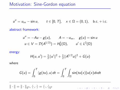
Motivation: Sine-Gordon equation

u′′ = uxx − sin u, t ∈ [0,T ], x ∈ Ω = (0, 1), b.c. + i.c.

abstract framework:

u′′ = −Au − g(u), A = −uxx , g(u) = sin u

u ∈ V = D(A1/2)) = H10 (Ω), u′ ∈ L2(Ω)

energy:H(u, u′) = 1

2‖u′‖2 + 1

2‖A1/2u‖2 + G (u)

where

G (u) =

∫ T

0〈g(tu), u〉dt =

∫ T

0

∫

Ωsin(tu(x))u(x)dxdt

‖ · ‖ = ‖ · ‖L2 , 〈·, ·〉 = 〈·, ·〉L2

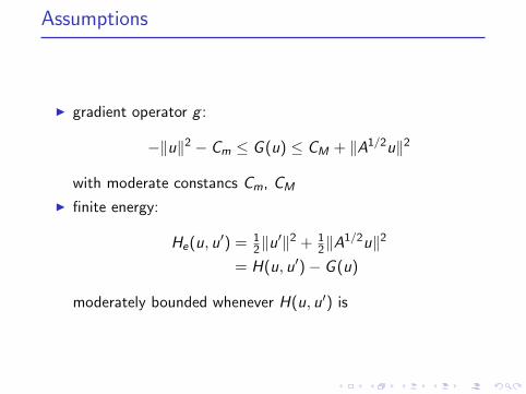
Assumptions

gradient operator g :

−‖u‖2 − Cm ≤ G (u) ≤ CM + ‖A1/2u‖2

with moderate constancs Cm, CM

finite energy:

He(u, u′) = 1

2‖u′‖2 + 1

2‖A1/2u‖2

= H(u, u′) − G (u)

moderately bounded whenever H(u, u′) is

Some facts

A unbouded operator

u highly oscillatory in time (temporal derivaties not bounded)

u satisfies finite energy assumptions

high frequencies cause small time steps

energy conservation

Spatial discretization: oscillatory ode

second-order ode

y ′′ + Ω2Ny = g(y), y(0) = y0, y ′(0) = y ′

0

withΩN = A

1/2N ,

finite energy

H(y , y ′) = 12‖y

′‖2 + 12yTΩ2

Ny ≤ 12K

Ω2 = AN sym. pos. semidef.

Gautschi-type exponential integrator

y ′′ + Ω2(t, y)y = g(y), y(0) = y0 , y ′(0) = y ′0

for constant g and Ω, exact solution satisfies

y(t+h)−2y(t)+y(t−h) = h2ψ(hΩ)(

g−Ω2y(t))

, ψ(x) = sinc2 x

2

(variation-of-constants formula)

Gautschi-type exponential integrator

yn+1 − 2yn + yn−1 = h2ψ(hΩn)(

gn − Ω2n yn

)

, Ωn = Ω(tn, yn)

(Verlet for Ω = 0)

Gautschi-type exponential integrator

y ′′ + Ω2(t, y)y = g(y), y(0) = y0 , y ′(0) = y ′0

for constant g and Ω, exact solution satisfies

y(t+h)−2y(t)+y(t−h) = h2ψ(hΩ)(

g−Ω2y(t))

, ψ(x) = sinc2 x

2

(variation-of-constants formula)

Gautschi-type exponential integrator

yn+1 − 2yn + yn−1 = h2ψ(hΩn)(

gn − Ω2n yn

)

, Ωn = Ω(tn, yn)

(Verlet for Ω = 0)

choice of gn?

Gautschi-type exponential integrator

yn+1 − 2yn + yn−1 = h2ψ(hΩn)(

gn − Ω2n yn

)

obvious choice: gn = g(yn) −→ Gautschi ’61

resonance problems for hωk ≈ jπ, ωk eigenvalue of Ωn

better choice: gn = g(φ(hΩn)yn), φ filter function

φ(0) = 1 , φ(kπ) = 0 , k = 1, 2, 3, . . .

convergence result: (H., Lubich, ’99, Grimm ’02, ’05)Assumptions: g smooth, bounded energy:

‖yn − y(tn)‖ ≤ h2C (tn), C (tn) ∼ etnL

Effect of filter function

10−3

10−2

10−1

100

10−6

10−5

10−4

10−3

10−2

10−1

without φ with φ

Numerical example: time step h = 0.02

Verlet scheme

128 Fourier modes 512 Fourier modes 2048 Fourier modes

0 0.5 1−0.05

0

0.05

0 0.5 1−0.05

0

0.05

Gautschi-type exponential integrator

0 0.5 1−0.05

0

0.05

0 0.5 1−0.05

0

0.05

0 0.5 1−0.05

0

0.05

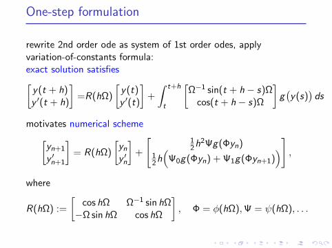
One-step formulation

rewrite 2nd order ode as system of 1st order odes, applyvariation-of-constants formula:exact solution satisfies

[

y(t + h)y ′(t + h)

]

=R(hΩ)

[

y(t)y ′(t)

]

+

∫ t+h

t

[

Ω−1 sin(t + h − s)Ωcos(t + h − s)Ω

]

g(

y(s))

ds

motivates numerical scheme

[

yn+1

y ′n+1

]

= R(hΩ)

[

yn

y ′n

]

+

[

12h2Ψg(Φyn)

12h

(

Ψ0g(Φyn) + Ψ1g(Φyn+1))

]

,

where

R(hΩ) :=

[

cos hΩ Ω−1 sin hΩ−Ω sin hΩ cos hΩ

]

, Φ = φ(hΩ),Ψ = ψ(hΩ), . . .

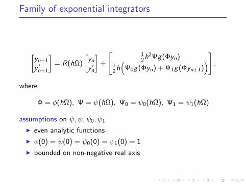
Family of exponential integrators

[

yn+1

y ′n+1

]

= R(hΩ)

[

yn

y ′n

]

+

[

12h2Ψg(Φyn)

12h

(

Ψ0g(Φyn) + Ψ1g(Φyn+1))

]

,

where

Φ = φ(hΩ), Ψ = ψ(hΩ), Ψ0 = ψ0(hΩ), Ψ1 = ψ1(hΩ)

assumptions on ψ,ψ, ψ0, ψ1

even analytic functions

φ(0) = ψ(0) = ψ0(0) = ψ1(0) = 1

bounded on non-negative real axis

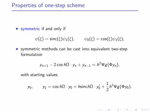
Properties of one-step scheme

symmetric if and only if

ψ(ξ) = sinc(ξ)ψ1(ξ), ψ0(ξ) = cos(ξ)ψ1(ξ),

symmetric methods can be cast into equivalent two-stepformulation

yn+1 − 2 cos hΩ · yn + yn−1 = h2Ψg(Φyn),

with starting values

y0, y1 = cos hΩ · y0 + hsinchΩ · y ′0 +

1

2h2Ψg(Φy0).

One- and two-step formulations, order

mollified impulse method(Garcıa-Archilla, Sanz-Serna, Skeel, 1998)

order 2 as one-step method with particular starting value y0, y1

as above order 1 as two-step method with exact starting values

Gautschi-type integrator(H., Lubich, 1998)

order 2 as two-step method for arbitrary starting values closeenough to exact solution

symmetric one-step formulation leads to ψ1 with singularitiesat integer multiples of π

Symplecticity

necessary and sufficient condition for one-step methods beingsymplecitic (Hairer, Lubich, Wanner, GNI, 2002)

ψ(ξ) = sinc(ξ)φ(ξ),

however (Hairer, Lubich, 2000)for Ω = ω > 0 and linear problems, i.e. g(y) = By , energy isconserved up to O(h) for all values of hω if and only if

ψ(ξ) = sinc2(ξ)φ(ξ)

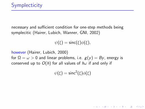
Symplecticity

necessary and sufficient condition for one-step methods beingsymplecitic (Hairer, Lubich, Wanner, GNI, 2002)

ψ(ξ) = sinc(ξ)φ(ξ),

however (Hairer, Lubich, 2000)for Ω = ω > 0 and linear problems, i.e. g(y) = By , energy isconserved up to O(h) for all values of hω if and only if

ψ(ξ) = sinc2(ξ)φ(ξ)

indicates that methods satisfying the latter condition are preferableto symplectic ones

Assumptions on filter functions

maxξ≥0

|χ(ξ)| ≤ M1, χ = φ, ψ, ψ0, ψ1

maxξ≥0

∣

∣

∣

∣

φ(ξ) − 1

ξ

∣

∣

∣

∣

≤ M2.

maxξ≥0

∣

∣

∣

∣

∣

1

sin ξ2

(

sinc2 ξ

2− ψ(ξ)

)

∣

∣

∣

∣

∣

≤ M3

maxξ≥0

∣

∣

∣

∣

∣

1

ξ sin ξ2

(sinc ξ − χ(ξ))

∣

∣

∣

∣

∣

≤ M4, χ = φ, ψ0, ψ1

[

yn+1

y ′n+1

]

= R(hΩ)

[

yn

y ′n

]

+

[

12h2Ψg(Φyn)

12h

(

Ψ0g(Φyn) + Ψ1g(Φyn+1))

]

,

Theorem (Grimm, H., 2006)

Assumptions;

exact solution y satisfies finite-energy condition

conditions on filter functions are satisfied

then

‖y(tn) − yn‖ ≤ h2C , t0 ≤ tn = t0 + nh ≤ t0 + T

where the constant C depends on T ,K ,M1, . . . ,M4, ‖g‖, ‖gy‖,and ‖gyy‖.

additional conditions on filter functions

‖y ′(tn) − y ′n‖ ≤ hC ′, t0 ≤ tn = t0 + nh ≤ t0 + T

Numerical examples

Fermi-Pasta-Ulam problem

stiffharmonic

softnonlinear

new choice of filter function (H., Grimm, ’06)

ψ(ξ) = sinc3(ξ), φ(ξ) = sinc(ξ)

order two

energy conserved up to O(h) for linear problems

Gautschi-type methods

ψ(ξ) φ(ξ)

A sinc2( 12ξ) 1 Gautschi, ’61

B sinc(ξ) 1 Deuflhard, ’79

C sinc(ξ)φ(ξ) sinc(ξ) Garcıa-Archilla et al., ’96

D sinc2( 12ξ) sinc(ξ)

(

1 + 13 sin2

(

12ξ

))

H., Lubich, ’98

E sinc2(ξ) 1 Hairer, Lubich, ’00

G sinc3(ξ) sinc(ξ) Grimm, H., ’06

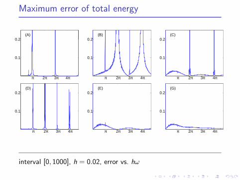
Maximum error of total energy

0.1

0.2

π 2π 3π 4π

(A)

0.1

0.2

π 2π 3π 4π

(B)

0.1

0.2

π 2π 3π 4π

(C)

0.1

0.2

π 2π 3π 4π

(D)

0.1

0.2

π 2π 3π 4π

(E)

0.1

0.2

π 2π 3π 4π

(G)

interval [0, 1000], h = 0.02, error vs. hω

Global error at t = 1

10−2

10−110

−6

10−4

10−2

100

(A)

10−2

10−110

−6

10−4

10−2

100

(B)

10−2

10−110

−6

10−4

10−2

100

(C)

10−2

10−110

−6

10−4

10−2

100

(D)

10−2

10−110

−6

10−4

10−2

100

(E)

10−2

10−110

−6

10−4

10−2

100

(G)

error vs. step size, ω = 1000

Maximum deviation of oscillatory energy

0.1

0.2

π 2π 3π 4π

(A)

0.1

0.2

π 2π 3π 4π

(B)

0.1

0.2

π 2π 3π 4π

(C)

0.1

0.2

π 2π 3π 4π

(D)

0.1

0.2

π 2π 3π 4π

(E)

0.1

0.2

π 2π 3π 4π

(G)

interval [0, 1000], h = 0.02, error vs. hω

Comments on new method

order 2 (according to theorem)

nearly conserved energy (for linear problems according toHairer, Lubich, ’00)

no resonances for oscillatory energy (surprise, because there isno method which uniformely conserves oscillatory energy oninterval of length > 2π for linear problems, Hairer, Lubich ’00)

Sketch of proof

substitute exact solution into numerical scheme −→ defects

derive expressions for defects

substract numerical solution, obtain error recursion (discretevariation-of-constants formula)

use explicit expression for defects to bound all sums arising

apply Gronwall Lemma

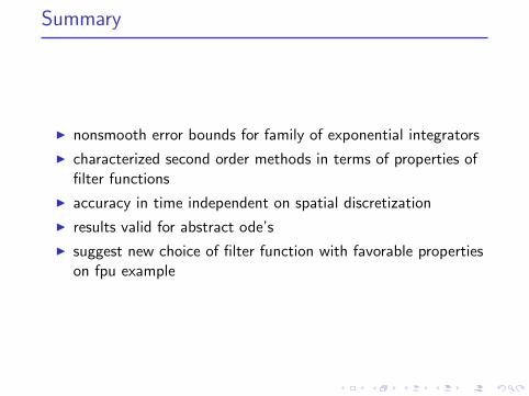
Summary

nonsmooth error bounds for family of exponential integrators

characterized second order methods in terms of properties offilter functions

accuracy in time independent on spatial discretization

results valid for abstract ode’s

suggest new choice of filter function with favorable propertieson fpu example