Numerical Integrators for Highly Oscillatory Hamiltonian ...jahnke/media/cojalolu.pdf · Numerical Integrators for Highly Oscillatory Hamiltonian Systems: A Review David Cohen1, Tobias

Numerical Integrators for Highly Oscillatory

Hamiltonian Systems: A Review

David Cohen1, Tobias Jahnke2, Katina Lorenz1, and Christian Lubich1

1 Mathematisches Institut, Univiversitat Tubingen, 72076 Tubingen. Cohen,Lorenz, [email protected]

2 Freie Universitat Berlin, Institut fur Mathematik II, BioComputing Group,Arnimallee 2–6, 14195 Berlin. [email protected]

Summary. Numerical methods for oscillatory, multi-scale Hamiltonian systems arereviewed. The construction principles are described, and the algorithmic and ana-lytical distinction between problems with nearly constant high frequencies and withtime- or state-dependent frequencies is emphasized. Trigonometric integrators forthe first case and adiabatic integrators for the second case are discussed in moredetail.

1 Introduction

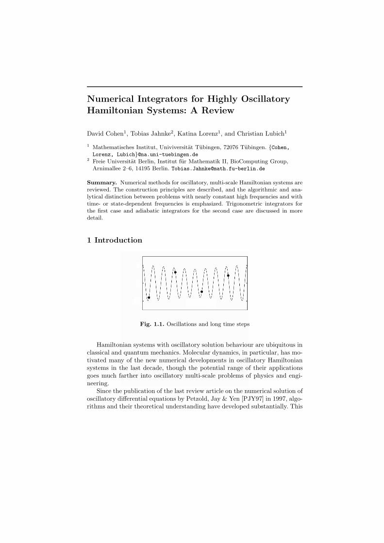
Fig. 1.1. Oscillations and long time steps

Hamiltonian systems with oscillatory solution behaviour are ubiquitous inclassical and quantum mechanics. Molecular dynamics, in particular, has mo-tivated many of the new numerical developments in oscillatory Hamiltoniansystems in the last decade, though the potential range of their applicationsgoes much farther into oscillatory multi-scale problems of physics and engi-neering.

Since the publication of the last review article on the numerical solution ofoscillatory differential equations by Petzold, Jay & Yen [PJY97] in 1997, algo-rithms and their theoretical understanding have developed substantially. This

554 D. Cohen, T. Jahnke, K. Lorenz, Ch. Lubich

fact, together with the pleasure of presenting a final report after six years offunding by the DFG Priority Research Program 1095 on multiscale systems,have incited us to write the present review, which concentrates on Hamiltoniansystems. A considerably more detailed (and therefore much longer) accountthan given here, appears in the second edition of the book by Hairer, Lubich& Wanner [HLW06, pp. 471–565]. Numerical methods for oscillatory Hamil-tonian systems are also treated in the book by Leimkuhler & Reich [LR04,pp. 257–286], with a different bias from ours.

The outline of this review is as follows. Sect. 2 describes some classes of os-cillatory, multi-scale Hamiltonian systems, with the basic distinction betweenproblems with nearly constant and with varying high frequencies. Sect. 3shows the building blocks with which integrators for oscillatory systems havebeen constructed. As is illustrated in Fig. 1.1, the aim is to have methods thatcan take large step sizes, evaluating computationally expensive parts of thesystem more rarely than a standard numerical integrator which would resolvethe oscillations with many small time steps per quasi-period. Sect. 4 dealswith trigonometric integrators suited for problems with almost-constant highfrequencies, and Sect. 5 with adiabatic integrators for problems with time- orsolution-dependent frequencies.

2 Highly oscillatory Hamiltonian systems

We describe some problem classes, given in each case by a Hamiltonian func-tion H depending on positions q and momenta p (and possibly on time t).The canonical equations of motion p = −∇qH, q = ∇pH are to be integratednumerically.

2.1 Nearly constant high frequencies

The simplest example is, of course, the harmonic oscillator given by the Hamil-tonian function H(p, q) = 1

2p2 + 12ω2q2, with the second-order equation of

motion q = −ω2q. This is trivially solved exactly, a fact that can be exploitedfor constructing methods for problems with Hamiltonian

H(p, q) =1

2pT M−1p +

1

2qT Aq + U(q) (2.1)

with a positive semi-definite constant stiffness matrix A of large norm, with apositive definite constant mass matrix M (subsequently taken as the identitymatrix for convenience), and with a smooth potential U having moderatelybounded derivatives.

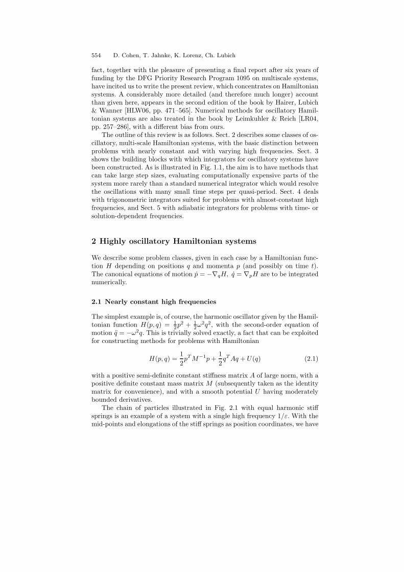
The chain of particles illustrated in Fig. 2.1 with equal harmonic stiffsprings is an example of a system with a single high frequency 1/ε. With themid-points and elongations of the stiff springs as position coordinates, we have

Integrators for Highly Oscillatory Hamiltonian Systems 555

stiffharmonic

softnonlinear

Fig. 2.1. Chain with alternating soft nonlinear and stiff linear springs

A =1

ε2

(0 00 I

), 0 < ε ≪ 1. (2.2)

Other systems have several high frequencies as in

A =1

ε2diag(0, ω1, . . . , ωm), 0 < ε ≪ 1, (2.3)

with 1 ≤ ω1 ≤ · · · ≤ ωm, or a wide range of low to high frequencies withoutgap as in spatial discretizations of semilinear wave equations.

In order to have near-constant high frequencies, the mass matrix need notnecessarily be constant. Various applications lead to Hamiltonians of the formstudied by Cohen [Coh06] (with partitions p = (p0, p1) and q = (q0, q1))

H(p, q) =1

2pT0 M0(q)

−1p0+1

2pT1 M−1

1 p1+1

2pT R(q)p+

1

2ε2qT1 A1q1+U(q) (2.4)

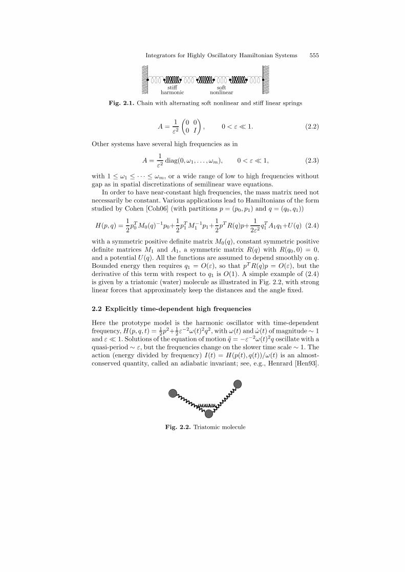
with a symmetric positive definite matrix M0(q), constant symmetric positivedefinite matrices M1 and A1, a symmetric matrix R(q) with R(q0, 0) = 0,and a potential U(q). All the functions are assumed to depend smoothly on q.Bounded energy then requires q1 = O(ε), so that pT R(q)p = O(ε), but thederivative of this term with respect to q1 is O(1). A simple example of (2.4)is given by a triatomic (water) molecule as illustrated in Fig. 2.2, with stronglinear forces that approximately keep the distances and the angle fixed.

2.2 Explicitly time-dependent high frequencies

Here the prototype model is the harmonic oscillator with time-dependentfrequency, H(p, q, t) = 1

2p2+ 12ε−2ω(t)2q2, with ω(t) and ω(t) of magnitude∼ 1

and ε ≪ 1. Solutions of the equation of motion q = −ε−2ω(t)2q oscillate with aquasi-period ∼ ε, but the frequencies change on the slower time scale ∼ 1. Theaction (energy divided by frequency) I(t) = H(p(t), q(t))/ω(t) is an almost-conserved quantity, called an adiabatic invariant; see, e.g., Henrard [Hen93].

Fig. 2.2. Triatomic molecule


Numerical methods designed for problems with nearly constant frequencies(and, more importantly, nearly constant eigenspaces) behave poorly on thisproblem, or on its higher-dimensional extension

H(p, q, t) =1

2pT M(t)−1p +

1

2ε2qT A(t)q + U(q, t), (2.5)

which describes oscillations in a mechanical system undergoing a slow drivenmotion. Here M(t) is a positive definite mass matrix, A(t) is a positive semi-definite stiffness matrix, and U(q, t) is a potential, all of which are assumed tobe smooth with derivatives bounded independently of the small parameter ε.This problem again has adiabatic invariants associated with each of its highfrequencies as long as the frequencies remain separated. However, on smalltime intervals where eigenvalues almost cross, rapid non-adiabatic transitionsmay occur, leading to further numerical challenges.

2.3 State-dependent high frequencies

Similar difficulties are present, and related numerical approaches have recentlybeen developed, in problems where the high frequencies depend on the posi-tion, as in the problem class studied analytically by Rubin & Ungar [RU57],Takens [Tak80], and Bornemann [Bor98]:

H(p, q) =1

2pT M(q)−1p +

1

ε2V (q) + U(q), (2.6)

with a constraining potential V (q) that takes its minimum on a manifoldand grows quadratically in non-tangential directions, thus penalizing motionsaway from the manifold. In appropriate coordinates we have

V (q) =1

2qT1 A(q0)q1 for q = (q0, q1)

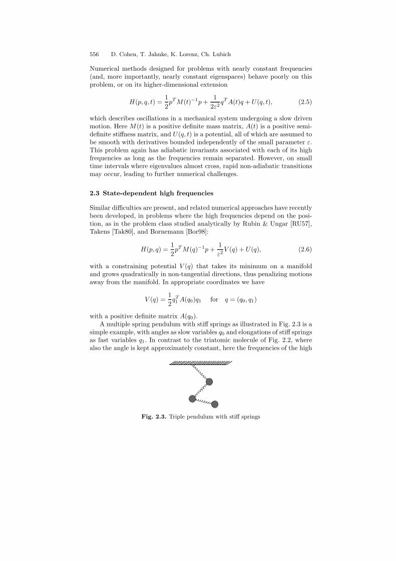
with a positive definite matrix A(q0).A multiple spring pendulum with stiff springs as illustrated in Fig. 2.3 is a

simple example, with angles as slow variables q0 and elongations of stiff springsas fast variables q1. In contrast to the triatomic molecule of Fig. 2.2, wherealso the angle is kept approximately constant, here the frequencies of the high

Fig. 2.3. Triple pendulum with stiff springs


oscillations depend on the angles which change during the motion. Differentphenomena occur, and different numerical approaches are appropriate for thetwo different situations.

As in the case of time-dependent frequencies, difficulties (numerical andanalytical) arise when eigenfrequencies cross or come close, which here can leadto an indeterminacy of the slow motion in the limit ε→ 0 (Takens chaos).

2.4 Almost-adiabatic quantum dynamics and

mixed quantum-classical molecular dynamics

A variety of new developments in the numerics of oscillatory problems withinthe last decade were spurred by problems from quantum dynamics; see,e.g., [BN*96, DS03, FL06, HL99b, HL99c, HL03, Jah03, Jah04, JL03, LT05,NR99, NS99, Rei99]. Though these problems can formally be viewed as be-longing to the classes treated above, it is worthwhile to state them separately:time-dependent quantum dynamics close to the adiabatic limit is describedby an equation

iεψ = H(t)ψ (2.7)

with a finite-dimensional hermitian matrix H(t) with derivatives of magnitude∼ 1 representing the quantum Hamiltonian. This is a complex Hamiltoniansystem with the time-dependent Hamiltonian function 1

2ψ∗H(t)ψ (considerthe real and imaginary parts of ψ as conjugate variables, and take an ε−1-scaled canonical bracket).

A widely used (though disputable) model of mixed quantum-classical me-chanics is the Ehrenfest model

q = −∇q

(ψ∗H(q)ψ

)

iεψ = H(q)ψ(2.8)

with a hermitian matrix H(q) depending on the classical positions q. This cor-responds to the Hamiltonian function 1

2pT p+ 12ψ∗H(q)ψ. The small parameter

ε here corresponds to the square root of the mass ratio of light (quantum) andheavy (classical) particles. While this is indeed small for electrons and nuclei,it is less so for protons and heavy nuclei. In the latter case an adiabatic reduc-tion to just a few eigenstates is not reasonable, and then one has to deal with aquantum Hamiltonian which is a discretization of a Laplacian plus a potentialoperator that depends on the classical position. Both cases show oscillatorybehaviour, but the appropriate numerical treatment is more closely relatedto that in Sects. 2.3 and 2.1 in the first and second case, respectively. Irre-spective of its actual physical modeling qualities, the Ehrenfest model is anexcellent model problem for studying numerical approaches and phenomenafor nonlinearly coupled slow and fast, oscillatory motion.


3 Building-blocks of long-time-step methods:

averaging, splitting, linearizing, corotating

We are interested in numerical methods that can attain good accuracy withstep sizes whose product with the highest frequency in the system need not besmall; see Fig. 1.1. A large variety of numerical methods to that purpose hasbeen proposed in the last decade, and a smaller variety among them has alsobeen carefully analysed. All these long-time-step and multiscale methods areessentially based on a handful of construction principles, combined in differentways. In addition to those described in the following, time-symmetry of themethod has proven to be extremely useful, whereas symplecticity appears toplay no essential role in long-time-step methods.

3.1 Averages

A basic principle underlying all long-time-step methods for oscillatory differ-ential equations is the requirement to avoid isolated pointwise evaluations ofoscillatory functions, but instead to rely on averaged quantities.

Following [HLW06, Sect. VIII.4], we illustrate this for a method for second-order differential equations such as those appearing in the previous section,

q = f(q), f(q) = f [slow](q) + f [fast](q). (3.1)

The classical Stormer-Verlet method with step size h uses a pointwise evalu-ation of f ,

qn+1 − 2qn + qn−1 = h2 f(qn), (3.2)

whereas the exact solution satisfies

q(t + h)− 2q(t) + q(t− h) = h2

∫ 1

−1

(1− |θ|) f(q(t + θh)

)dθ . (3.3)

The integral on the right-hand side represents a weighted average of the forcealong the solution, which will now be approximated. At t = tn, we replace

f(q(tn + θh)

)≈ f [slow](qn) + f [fast]

(u(θh)

)

where u(τ) is a solution of the differential equation

u = f [slow](qn) + f [fast](u) . (3.4)

We then have

h2

∫ 1

−1

(1−|θ|)(f [slow](qn)+ f [fast]

(u(θh)

))dθ = u(h)−2u(0)+u(−h) . (3.5)

For the differential equation (3.4) we assume the initial values u(0) = qn andu(0) = qn or simply u(0) = 0. This initial value problem is solved numeri-cally, e.g., by the Stormer-Verlet method with a micro-step size ±h/N with


N ≫ 1 on the interval [−h, h], yielding numerical approximations uN(±h) anduN (±h) to u(±h) and u(±h), respectively. No further evaluations of f [slow]

are needed for the computation of uN(±h) and uN (±h). This finally gives thesymmetric two-step method of Hochbruck & Lubich [HL99a],

qn+1 − 2qn + qn−1 = uN (h)− 2uN(0) + uN (−h) . (3.6)

The method can also be given a one-step formulation, see [HLW06, Sect. VIII.4].Further symmetric schemes using averaged forces were studied by Hochbruck& Lubich [HL99c] and Leimkuhler & Reich [LR01].

The above method is efficient if solving the fast equation (3.4) over thewhole interval [−h, h] is computationally less expensive than evaluating theslow force f [slow]. Otherwise, to reduce the number of function evaluations wecan replace the average in (3.5) by an average with smaller support,

qn+1 − 2qn + qn−1 = h2

∫ δ

−δ

K(θ)(f [slow](qn) + f [fast]

(u(θh)

))dθ (3.7)

with δ ≪ 1 and an averaging kernel K(θ) with integral equal to 1. This is fur-ther approximated by a quadrature sum involving the values f [fast]

(uN(mh/N)

)

with |m| ≤ M and 1 ≪ M ≪ N . The resulting method is an example of aheterogeneous multiscale method as proposed by E [E03] and Engquist & Tsai[ET05], with macro-step h and micro-step h/N . Method (3.7) is in betweenthe Stormer-Verlet method (3.2) (δ = 0) and the averaged-force method (3.6)(δ = 1).

In the above methods, the slow force is evaluated, somewhat arbitrarily,at the particular value qn approximating the oscillatory solution q(t). Instead,one might evaluate f [slow] at an averaged position qn, defined by solving ap-proximately an approximate equation

u = f [fast](u), u(0) = qn, u(0) = 0, and setting qn =

∫ δ

−δ

K(θ)u(θh) dθ,

with another averaging kernel K(θ) having integral 1. Such an approachwas first studied by Garcıa-Archilla, Sanz-Serna & Skeel [GSS99] for the im-pulse method (see below), and subsequently in [HL99a] for the averaged-forcemethod, in order to reduce the sensitivity to step size resonances in the nu-merical solution. For that purpose, it turned out that taking δ = 1 (or aninteger) is essential.

3.2 Splitting

The Stormer-Verlet method (see [HLW03]) can be interpreted as approximat-ing the flow ϕH

h of the system with Hamiltonian H(p, q) = T (p) + V (q) withT (p) = 1

2pT p by the symmetric splitting


ϕVh/2 ϕT

h ϕVh/2 .

In the situation of a potential V = V [fast] + V [slow], we may instead use adifferent splitting of H = (T + V [fast]) + V [slow] and approximate the flow ϕH

h

of the system by

ϕV [slow]

h/2 ϕT+V [fast]

h ϕV [slow]

h/2 .

This is the impulse method that was proposed in the context of moleculardynamics by Grubmuller, Heller, Windemuth & Schulten [GH*91] and Tuck-erman, Berne & Martyna [TBM92]:

1. kick: set p+n = pn − 1

2h∇V [slow](qn)

2. oscillate: solve q = −∇V [fast](q) with initial values (qn, p+n )

over a time step h to obtain (qn+1, p−

n+1)

3. kick: set pn+1 = p−n+1 − 12h∇V [slow](qn+1) .

(3.8)

Step 2 must in general be computed approximately by a numerical integratorwith a smaller time step. If the inner integrator is symplectic and symmetric,as it would be for the Stormer-Verlet method, then also the overall method issymplectic and symmetric.

Garcıa-Archilla, Sanz-Serna & Skeel [GSS99] mollify the impulse methodby replacing the slow potential V [slow](q) by a modified potential V [slow](q),where q represents a local average as considered above.

3.3 Variation of constants formula

A particular situation arises when the fast forces are linear, as in

q = −Ax + g(q) (3.9)

with a symmetric positive semi-definite matrix A of large norm. With Ω =A1/2, the exact solution satisfies

(q(t)q(t)

)=

(cos tΩ Ω−1 sin tΩ

−Ω sin tΩ cos tΩ

) (q0

q0

)(3.10)

+

∫ t

0

(Ω−1 sin(t− s)Ω

cos(t− s)Ω

)g(q(s)

)ds .

Discretizing the integral in different ways gives rise to various numericalschemes proposed in the literature for treating (3.9) (the earliest referencesare Hersch [Her58] and Gautschi [Gau61]). This also gives reinterpretationsof the methods discussed above when they are applied to (3.9). We consider aclass of trigonometric integrators that reduces to the Stormer-Verlet methodfor A = 0 and gives the exact solution for g = 0 [HLW06, Chap.XIII]:


qn+1 = coshΩ qn + Ω−1 sin hΩ qn +1

2h2Ψ g(Φqn) (3.11)

qn+1 = −Ω sin hΩ qn + coshΩ qn +1

2h(Ψ0 g(Φqn) + Ψ1 g(Φqn+1)

). (3.12)

Here Ψ = ψ(hΩ) and Φ = φ(hΩ), where the filter functions ψ and φ aresmooth, bounded, real-valued functions with ψ(0) = φ(0) = 1. Moreover,we have Ψ0 = ψ0(hΩ), Ψ1 = ψ1(hΩ) with even functions ψ0, ψ1 satisfyingψ0(0) = ψ1(0) = 1. The method is symmetric if and only if

ψ(ξ) = sinc(ξ)ψ1(ξ) , ψ0(ξ) = cos(ξ)ψ1(ξ) , (3.13)

where sinc(ξ) = sin(ξ)/ξ. In addition, the method is symplectic (for g =−∇U) if and only if

ψ(ξ) = sinc(ξ)φ(ξ) . (3.14)

The two-step form of the method reads

qn+1 − 2 cos(hΩ) qn + qn−1 = h2Ψg(Φqn) . (3.15)

Various methods of Sects. 3.1 and 3.2 can be written in this way, with differentfilters Ψ and Φ, when they are applied to (3.9):

ψ(ξ)= sinc2(12ξ) φ(ξ)=1 Gautschi [Gau61] and averaged method (3.6)

ψ(ξ)= sinc(ξ) φ(ξ)=1 Deuflhard [Deu79] and impulse method (3.8)ψ(ξ)= sinc2(ξ) φ(ξ)= sinc(ξ) Garcıa-Archilla & al. [GSS99]: mollified i.m.ψ(ξ)= sinc2(ξ) φ(ξ)=1 Hairer & Lubich [HL00]ψ(ξ)= sinc3(ξ) φ(ξ)= sinc(ξ) Grimm & Hochbruck [GH06]

As will be seen in Sect. 4, the choice of the filter functions has a substantialinfluence on the long-time properties of the method.

3.4 Transformation to corotating variables

For problems where the high frequencies and the corresponding eigenspacesdepend on time or on the solution, as in (2.5)–(2.8), it is useful to transformto corotating variables in the numerical treatment.

We illustrate the basic procedure for Schrodinger-type equations (2.7) witha time-dependent real symmetric matrix H(t) changing on a time scale∼ 1, forwhich the solutions are oscillatory with almost-period ∼ ε. A time-dependentlinear transformation η(t) = Tε(t)ψ(t) takes the system to the form

η(t) = Sε(t) η(t) with Sε = TεT−1ε − i

εTεHT−1

ε . (3.16)

A first approach is to freeze H(t) ≈ H∗ over a time step and to choose thetransformation


−1 0 1−1

0

1

q1(t)

time t−1 0 1

−0.01

0

0.01

real part of η1(t)

time t0.95 1

−1

0

1x 10

−3

real part of η1(t)

(zoomed)

time t

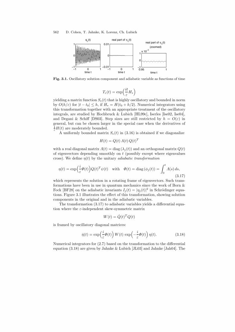
Fig. 3.1. Oscillatory solution component and adiabatic variable as functions of time

Tε(t) = exp( it

εH∗

)

yielding a matrix function Sε(t) that is highly oscillatory and bounded in normby O(h/ε) for |t− t0| ≤ h, if H∗ = H(t0 + h/2). Numerical integrators usingthis transformation together with an appropriate treatment of the oscillatoryintegrals, are studied by Hochbruck & Lubich [HL99c], Iserles [Ise02, Ise04],and Degani & Schiff [DS03]. Step sizes are still restricted by h = O(ε) ingeneral, but can be chosen larger in the special case when the derivatives of1εH(t) are moderately bounded.

A uniformly bounded matrix Sε(t) in (3.16) is obtained if we diagonalize

H(t) = Q(t)Λ(t)Q(t)T

with a real diagonal matrix Λ(t) = diag (λj(t)) and an orthogonal matrix Q(t)of eigenvectors depending smoothly on t (possibly except where eigenvaluescross). We define η(t) by the unitary adiabatic transformation

η(t) = exp( i

εΦ(t)

)Q(t)T ψ(t) with Φ(t) = diag (φj(t)) =

∫ t

0

Λ(s) ds,

(3.17)which represents the solution in a rotating frame of eigenvectors. Such trans-formations have been in use in quantum mechanics since the work of Born &Fock [BF28] on the adiabatic invariants Ij(t) = |ηj(t)|2 in Schrodinger equa-tions. Figure 3.1 illustrates the effect of this transformation, showing solutioncomponents in the original and in the adiabatic variables.

The transformation (3.17) to adiabatic variables yields a differential equa-tion where the ε-independent skew-symmetric matrix

W (t) = Q(t)T Q(t)

is framed by oscillatory diagonal matrices:

η(t) = exp( i

εΦ(t)

)W (t) exp

(− i

εΦ(t)

)η(t). (3.18)

Numerical integrators for (2.7) based on the transformation to the differentialequation (3.18) are given by Jahnke & Lubich [JL03] and Jahnke [Jah04]. The


simplest of these methods freezes the slow variables η(t) and W (t) at the mid-point of the time step, makes a piecewise linear approximation to the phaseΦ(t), and then integrates the resulting system exactly over the time step. Thisgives the following adiabatic integrator :

ηn+1 = ηn + hB(tn+1/2)1

2(ηn + ηn+1) with (3.19)

B(t) =

(exp

(− i

ε

(φj(t)− φk(t)

))sinc

( h

2ε

(λj(t)− λk(t)

))wjk(t)

)

j,k

.

More involved – and substantially more accurate – methods use a Neumannor Magnus expansion in (3.18) and a quadratic phase approximation. Numer-ical challenges arise near avoided crossings of eigenvalues, where η(t) remainsno longer nearly constant and a careful choice of step size selection strat-egy is needed in order to follow the non-adiabatic transitions; see [JL03] and[HLW06, Chap. XIV].

The extension of this approach to (2.5), (2.6), and (2.8) is discussed inSect. 5. The transformation to adiabatic variables is also a useful theoreticaltool for analysing the error behaviour of multiple time-stepping methods ap-plied to these problems in the original coordinates, such as the impulse andmollified impulse methods considered in Sect. 3.2; see [HLW06, Chap. XIV].

4 Trigonometric integrators for problems with nearly

constant frequencies

A good understanding of the behaviour of numerical long-time-step methodsover several time scales has been gained for Hamiltonian systems with almost-constant high frequencies as considered in Sect. 2.1. We here review resultsfor single-frequency systems (2.1) with (2.2) (and M = I) from Hairer &Lubich [HL00] and [HLW06, Chap. XIII], with the particle chain of Fig. 2.1serving as a concrete example. The variables are split as q = (q0, q1) accordingto the blocks in (2.2). We consider initial conditions for which the total energyH(p, q) is bounded independently of ε,

H(p(0), q(0)) ≤ Const.

The principal theoretical tool is a modulated Fourier expansion of both theexact and the numerical solution,

q(t) =∑

k zk(t) eikt/ε, (4.1)

an asymptotic multiscale expansion with coefficient functions zk(t) changingon the slow time scale 1, which multiply exponentials that oscillate with fre-quency 1/ε. The system determining the coefficient functions turns out to


have a Hamilton-type structure with formal invariants close to the total andoscillatory energies.

The results on the behaviour of trigonometric integrators (3.15) on differ-ent time scales have been extended from single- to multi-frequency systems(possibly with resonant frequencies) by Cohen, Hairer & Lubich [CHL05], andto systems (2.4) with non-constant mass matrix by Cohen [Coh04, Coh06].

4.1 Time scale ε

On this time scale the system (2.1) with (2.2) only shows near-harmonic oscil-lations with frequency 1/ε and amplitude O(ε) in the fast variables q1, whichare well reproduced by just any numerical integrator.

4.2 Time scale ε0

This is the time scale of motion of the slow variables q0 under the influenceof the potential U(q). Here it is of interest to have an error in the numericalmethods which is small in the step size h and uniform in the product of thestep size with the high frequency 1/ε. The availability of such uniform errorbounds depends on the behaviour of the filter functions ψ and φ in (3.15) atintegral multiples of π. Under the conditions

ψ(2kπ) = ψ′(2kπ) = 0, ψ((2k − 1)π) = 0, φ(2kπ) = 0 (4.2)

for k = 1, 2, 3, . . . , it is shown in [HLW06, Chap. XIII.4] that the error aftern time steps is bounded by

‖qn − q(nh)‖ ≤ C h2, ‖qn − q(nh)‖ ≤ C h for nh ≤ Const., (4.3)

with C independent of h/ε and of bounds of derivatives of the highly oscilla-tory solution.

Error bounds without restriction of the product of the step size with thefrequencies are given for general positive semi-definite matrices A in (2.1) byGarcıa-Archilla, Sanz-Serna & Skeel [GSS99] for the mollified impulse method(ψ(ξ) = sinc2(ξ), φ(ξ) = sinc(ξ)), by Hochbruck & Lubich [HL99a] andGrimm [Gri05a] for Gautschi-type methods (ψ(ξ) = sinc2(ξ/2) and suitableφ), and most recently by Grimm & Hochbruck [GH06] for general A andgeneral classes of filter functions ψ and φ.

4.3 Time scale ε−1

An energy exchange between the stiff springs in the particle chain takes placeon the slower time scale ε−1. To describe this in mathematical terms, let q1,j

be the jth component of the fast position variables q1, and consider

Ij =1

2q21,j +

1

2ε2q21,j ,


which in the example represents the harmonic energy in the jth stiff spring.The quantities Ij change on the time scale ε−1. To leading order in ε, theirchange is described by a differential equation that determines the coefficientof eit/ε in the modulated Fourier expansion (4.1). It turns out that for atrigonometric method (3.15), the differential equation for the correspondingcoefficient in the modulated Fourier expansion of the numerical solution isconsistent with that of the exact solution for all step sizes if and only if

ψ(ξ)φ(ξ) = sinc(ξ) for all ξ ≥ 0.

It is interesting to note that this condition for correct numerical energy ex-change is in contradiction with the condition (3.14) of symplecticity of themethod, with the only exception of the impulse method, given by ψ =sinc, φ = 1. That method, however, does not satisfy (4.2) and is in factextremely sensitive to near-resonances between frequency and step size (h/εnear even multiples of π). A way out of these difficulties is to consider trigono-metric methods with more than one force evaluation per time step, as is shownin [HLW06, Chap. XIII].

In Fig. 4.1 we show the energy exchange of three numerical methods forthe particle chain of Fig. 2.1, with ε = 0.02 and with potential and initialdata as in [HLW06, p. 22]. At t = 0 only the first stiff spring is elongated,the other two being at rest position. The harmonic energies I1, I2, I3, theirsum I = I1 + I2 + I3, and the total energy H (actually H − 0.8 for graphicalreasons) are plotted along the numerical solutions of the following methods,with step sizes h = 0.015 and h = 0.03:

(A) impulse method (ψ = sinc, φ = 1)(B) mollified impulse method (ψ = sinc2, φ = sinc)(C) heterogeneous multiscale method (3.7) with δ =

√ε.

50 100 1500

1

50 100 1500

1

50 100 1500

1

50 100 1500

1

50 100 1500

1

50 100 1500

1

(A) H

I

(B) H

I

(C) H

I

Fig. 4.1. Energy exchange between the stiff springs for methods (A)-(C), withh = 0.015 (upper) and h = 0.03 (lower), for ε = 0.02


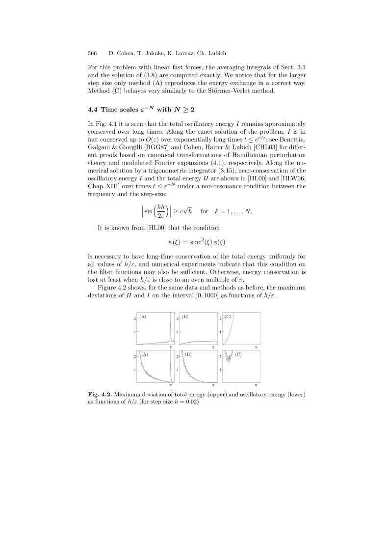
For this problem with linear fast forces, the averaging integrals of Sect. 3.1and the solution of (3.8) are computed exactly. We notice that for the largerstep size only method (A) reproduces the energy exchange in a correct way.Method (C) behaves very similarly to the Stormer-Verlet method.

4.4 Time scales ε−N with N ≥ 2

In Fig. 4.1 it is seen that the total oscillatory energy I remains approximatelyconserved over long times. Along the exact solution of the problem, I is infact conserved up to O(ε) over exponentially long times t ≤ ec/ε; see Benettin,Galgani & Giorgilli [BGG87] and Cohen, Hairer & Lubich [CHL03] for differ-ent proofs based on canonical transformations of Hamiltonian perturbationtheory and modulated Fourier expansions (4.1), respectively. Along the nu-merical solution by a trigonometric integrator (3.15), near-conservation of theoscillatory energy I and the total energy H are shown in [HL00] and [HLW06,Chap. XIII] over times t ≤ ε−N under a non-resonance condition between thefrequency and the step-size:

∣∣∣ sin(kh

2ε

)∣∣∣ ≥ c√

h for k = 1, . . . , N.

It is known from [HL00] that the condition

ψ(ξ) = sinc2(ξ)φ(ξ)

is necessary to have long-time conservation of the total energy uniformly forall values of h/ε, and numerical experiments indicate that this condition onthe filter functions may also be sufficient. Otherwise, energy conservation islost at least when h/ε is close to an even multiple of π.

Figure 4.2 shows, for the same data and methods as before, the maximumdeviations of H and I on the interval [0, 1000] as functions of h/ε.

.1

.2

.1

.2

.1

.2

.1

.2

.1

.2

.1

.2

π

(A)

π

(B)

π

(C)

π

(A)

π

(B)

π

(C)

Fig. 4.2. Maximum deviation of total energy (upper) and oscillatory energy (lower)as functions of h/ε (for step size h = 0.02)


5 Adiabatic integrators for problems with varying

frequencies

Adiabatic integrators are a novel class of numerical integrators that have beendevised in [JL03, Jah04, Jah03, LJL05, Lor06, HLW06] for various kinds ofoscillatory problems with time- or solution-dependent high frequencies, in-cluding (2.5)–(2.8). These integrators have in common that the oscillatorypart of the problem is transformed to adiabatic variables (cf. Sect. 3.4) andthe arising oscillatory integrals are computed analytically or approximated byan appropriate expansion. The methods allow to integrate these oscillatorydifferential equations with large time steps in the adiabatic regime of well-separated frequencies and follow non-adiabatic transitions with adaptivelyrefined step sizes.

5.1 Adiabatic integrators for quantum-classical molecular

dynamics

Following Jahnke [Jah03], we sketch how to construct a symmetric long-time-step method for problem (2.8), which couples in a nonlinear way slow motionand fast oscillations with frequencies depending on the slow variables.

Proceeding as in Sect. 3.4, the quantum system is transformed to adiabaticvariables by

η(t) = exp

(i

εΦ(t)

)Q

(q(t)

)Tψ(t) , (5.1)

where H(q) = Q(q)Λ(q)Q(q)T is a smooth eigendecomposition of the Hamil-tonian and

Φ(t) =

∫ t

t0

Λ(q(s)

)ds, Φ = diag(φj) (5.2)

is the phase matrix, a diagonal matrix containing the time integrals over theeigenvalues λj(q(t)) along the classical trajectory. Inserting (5.1) into (2.8)yields the new equations of motion

q = −η∗ exp

(i

εΦ

)K(q) exp

(− i

εΦ

)η, (5.3)

η = exp

(i

εΦ

)W (q, q) exp

(− i

εΦ

)η (5.4)

with the tensor K(q) and skew-symmetric matrix W (q, q) given as

K(q) = Q(q)T∇qH(q)Q(q),

W(q, q

)=

(d

dtQ

(q))T

Q(q)

=(∇qQ

(q)q)T

Q(q). (5.5)


Equations (5.3) and (5.4) can be restated as

q = −η∗

(E(Φ) •K(q)

)η, (5.6)

η =(E(Φ) •W (q, q)

)η. (5.7)

where • means entrywise multiplication, and E(Φ) denotes the matrix

E(Φ) =(ejk(Φ)

), ejk(Φ) = exp

(i

ε(φj − φk)

). (5.8)

The classical equation can be integrated using the averaging technique fromSect. 3. We insert (5.6) into (3.3) and, in order to approximate the integral,keep the smooth variables η(t) and K(q(t)) fixed at the midpoint tn of theinterval [tn−1, tn+1]. Since more care is necessary for the oscillating exponen-tials, we replace Φ by the linear approximation

Φ(tn + θh) ≈ Φ(tn) + θhΛ(q(tn)

). (5.9)

These modifications yield the averaged Stormer-Verlet method of [Jah03]:

qn+1 − 2qn + qn−1 = −h2 η∗

n

(E(Φn) • I(qn) •K(qn)

)ηn (5.10)

with I(qn) =

∫ 1

−1

(1− |θ|)E(θhΛ(qn)

)dθ.

The matrix of oscillatory integrals I(qn) can be computed analytically: itsentries Ijk(qn) are given by

Ijk(qn) =

∫ 1

−1

(1− |θ|) exp(iθξjk) dθ = sinc2(12ξjk)

with ξjk =h

ε

(λj(qn)− λk(qn)

). (5.11)

Note that in the (computationally uninteresting) small-time-step limit h/ε →0 the integrator (5.10) converges to the Stormer-Verlet method.

The easiest way to approximate the quantum vector η(t) is to keepη(t) ≡ η(0) simply constant. According to the quantum adiabatic theorem[BF28] the resulting error is only O(ε) as long as the eigenvalues of H(q(t))are well separated and the eigendecomposition remains smooth. A more re-liable method, which in its variable-time-step version follows non-adiabatictransitions in η occurring near avoided crossings of eigenvalues, is obtainedby integrating Eq. (5.7) from tn − h to tn + h, using the linear approxima-tion (5.9) for Φ(t), and freezing the slow coupling matrix W (q(t), q(t)) at themidpoint tn. This yields the adiabatic integrator from [Jah03],


ηn+1 − ηn−1 =2h(E(Φn) • J (qn) •Wn

)ηn (5.12)

with J (qn) =1

2

∫ 1

−1

E(θhΛ(qn)

)dθ.

The (j, k)-entry of the matrix of oscillatory integrals J (qn) is simply

Jjk(qn) =1

2

∫ 1

−1

exp(iθξjk) dθ = sinc ξjk.

The explicit midpoint rule is recovered in the limit h/ε → 0. The derivativecontained in (5.5) and the integral in (5.2) are not known explicitly but canbe approximated by the corresponding symmetric difference quotient and thetrapezoidal rule, respectively. These approximations are denoted by Wn andΦn in the above formulas.

The approximation properties of method (5.10), (5.12) for large step sizesup to h ≤ √ε are analysed in [Jah03]. A discrete quantum-adiabatic theoremis established, which plays an important role in the error analysis.

5.2 Adiabatic integrators for problems with time-dependent

frequencies

Adiabatic integrators for mechanical systems with a time-dependent multi-scale Hamiltonian (2.5) are presented in [HLW06, Chap. XIV] and [Lor06],following up on previous work by Lorenz, Jahnke & Lubich [LJL05] for sys-tems (2.5) with M(t) ≡ I and A(t) a symmetric positive definite matrix. Tosimplify the presentation, we ignore in the following the slow potential andset U ≡ 0.

The approach is based on approximately separating the fast and slow timescales by a series of time-dependent canonical linear coordinate transforma-tions, which are done numerically by standard numerical linear algebra rou-tines. The procedure can be sketched as follows:

• The Cholesky decomposition M(t) = C(t)−T C(t) and the transformationq → C(t)q change the Hamiltonian in such a way that the new mass matrixis the identity.

• The eigendecomposition

A(t) = Q(t)

(0 00 Ω(t)2

)Q(t)T , Ω(t) = diag(ωj(t))

of the symmetric stiffness matrix A(t) allows to split the positions q =(q0, q1) and momenta p = (p0, p1) into slow and fast variables q0, p0 andq1, p1, respectively.

• The fast positions and momenta are rescaled by ε−1/2Ω(t)1/2 and byε1/2Ω(t)−1/2, respectively.


• The previous transforms produce a non-separable term qT K(t)p in theHamiltonian. One block of the matrix K(t) is of order O(ε−1/2) and hasto be removed by one more canonical transformation.

The Hamiltonian in the new coordinates p = (p0, p1) and q = (q0, q1) thentakes the form

H(p, q, t) =1

2pT0 p0 +

1

2εpT1 Ω(t)p1 +

1

2εqT1 Ω(t)q1 + qT L(t)p +

1

2qT S(t)q

with a lower block-triangular matrix L and a symmetric matrix S of the form

L =

(L00 0

ε1/2L10 L11

), S =

(S00 ε1/2S01

ε1/2S10 εS11

).

Under the condition of bounded energy, the fast variables q1 and p1 are nowof order O(ε1/2). The equations of motion read

p0 = f0(p, q, t)

q0 = p0 + g0(q, t)

(p1

q1

)=

1

ε

(0 −Ω(t)

Ω(t) 0

) (p1

q1

)+

(f1(p, q, t)g1(q, t)

)

with functions(

f0

f1

)= −L(t)p− S(t)q,

(g0

g1

)= L(t)T q,

which are bounded uniformly in ε. The oscillatory part now takes the form ofa skew-symmetric matrix multiplied by 1/ε, similar to (2.7). We diagonalizethis matrix and define the diagonal phase matrix Φ as before:

(0 −Ω(t)

Ω(t) 0

)= ΓiΛ(t)Γ ∗, Γ =

1√2

(I I−iI iI

), (5.13)

Λ(t) =

(Ω(t) 0

0 −Ω(t)

), Φ(t) =

∫ t

t0

Λ(s) ds. (5.14)

The transformation to adiabatic variables is now taken as

η = ε−1/2 exp(− i

εΦ(t)

)Γ ∗

(p1

q1

)(5.15)

with the factor ε−1/2 introduced such that η = O(1). The equations of motionbecome

p0 = −L00p0 − S00q0 − εS01Q1η

q0 = p0 + LT00q0 + εLT

10Q1η (5.16)


for the slow variables, and

η = exp(− i

εΦ)

W exp( i

εΦ)

η − P ∗

1

(L10p0 + S10q0

)(5.17)

for the adiabatic variables, where

W = Γ ∗

(−L11 −εS11

0 LT11

)Γ,

(P1

Q1

)= Γ exp

( i

εΦ).

Slow and fast degrees of freedom are only weakly coupled, because in theslow equations (5.16) the fast variable η always appears with a factor ε. Theoscillatory part has the familiar form of a coupling matrix framed by oscilla-tory exponentials, cf. (3.18) and (5.4). Under a separation condition for thefrequencies ωj(t), the fact that the diagonal of W is of size O(ε) implies thatthe expressions Ij = |ηj |2 are adiabatic invariants. Ij is the action (energydivided by frequency)

Ij =1

ωj

(1

2p21,j +

ω2j

2ε2q21,j

).

An adiabatic integrator for (2.5) is obtained by the following splitting (fordetails see [HLW06, Chap.XIV] and Lorenz [Lor06]):

1. Propagate the slow variables (p0, q0) with a half-step of the symplecticEuler method. For the oscillatory function Q1(t), replace the evaluationat tn+1/2 = tn + h/2 by the average

Q−

1 ≈2

h

∫ tn+1/2

tn

Q1(t) dt,

obtained with a linear approximation of the phase Φ(t) and analytic com-putation of the integral.

2. Propagate the adiabatic variable η with a full step of a method of type(3.19) for (5.17).

3. Propagate the slow variables (p0, q0) with a half-step of the adjoint sym-plectic Euler method, with an appropriate average of Q1(t).

The approximation properties of this method are analyzed in [HLW06, Chap.XIV],where it is shown that the error over bounded time intervals, in the originalvariables of (2.5), is of order O(h2) in the positions and O(h) in the momenta,uniformly in ε for h ≤ √ε. Numerical comparisons with other methods illus-trate remarkable benefits of this approach [Lor06, LJL05].

We present numerical illustrations from Lorenz [Lor06] for the time-dependent Hamiltonian (2.5) with M(t) ≡ I and

A(t) =

(t + 3 δ

δ 2t + 3

)2


−1 0 1

1

2

3

4

5

δ = 1

time t

eigen

value

s

−1 0 1

1

2

3

4

5

δ = 0.1

time t−1 0 1

1

2

3

4

5

δ = 0.01

time t

−1 0 1

0

5

10

15

20

25

δ = 1

time t

norm

of dQ

−1 0 1

0

5

10

15

20

25

δ = 0.1

time t−1 0 1

0

5

10

15

20

25

δ = 0.01

time t

Fig. 5.1. Frequencies ωj (upper) and ‖Q‖ (lower) for δ = 1, 0.1, 0.01

on the time interval [−1, 1]. The behaviour of the components of the solutionq(t) and the adiabatic variable η(t) are as in Fig. 3.1 for δ = 1 and η = 0.01.

Figure 5.1 shows the frequencies and the norm of the time derivative ofthe matrix Q(t) that diagonalizes A(t) for various values of the parameter δ.For small values of δ, the frequencies approach each other to O(δ) at t = 0,and ‖Q(0)‖ ∼ δ−1. This behaviour affects the adiabatic variables ηj(t), as isshown in Fig. 5.2.

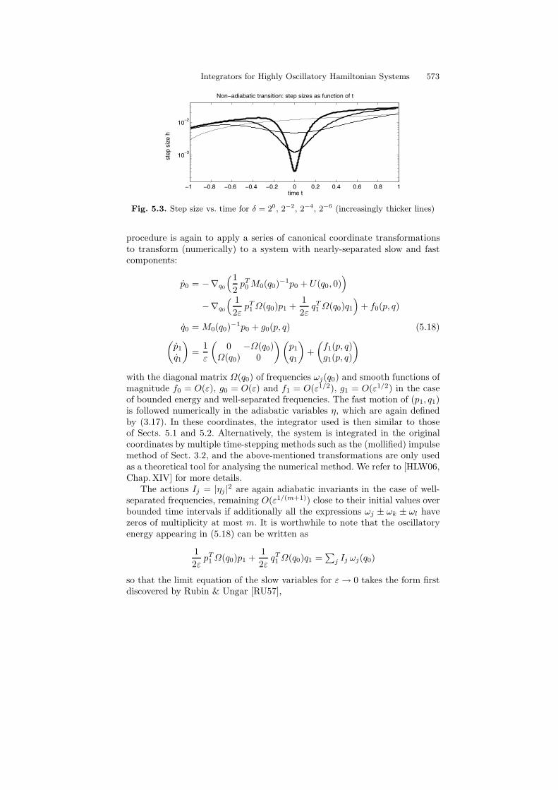
For δ ∼ ε1/2, there appears an O(1) change in η in an O(δ) neighbourhoodof t = 0, and for smaller values of δ the components of η essentially exchangetheir values; cf. Zener [Zen32] for the analogous situation in Schrodinger-type equations (2.7). Small step sizes are needed near t = 0 to resolve thisbehaviour. Figure 5.3 shows the step sizes chosen by a symmetric adaptivestep selection algorithm described in [HLW06, Chap. XIV] for different valuesof δ. Errors of similar size are obtained in each case.

5.3 Integrators for motion under a strong constraining force

The methods and techniques of the previous subsection can be extended toproblems (2.6) with solution-dependent high frequencies [HLW06, Lor06]. The

−1 0 1

0

0.2

0.4

0.6

δ = 1

time t

−1 0 1

0

0.2

0.4

0.6

δ = 0.1

time t

−1 0 1

0

0.2

0.4

0.6

δ = 0.01

time t−1 0 1

0

0.2

0.4

0.6

δ = 0.001

time t

Fig. 5.2. Adiabatic variables ηj as functions of time


−1 −0.8 −0.6 −0.4 −0.2 0 0.2 0.4 0.6 0.8 1

10−3

10−2

Non−adiabatic transition: step sizes as function of t

time t

ste

p s

ize

h

Fig. 5.3. Step size vs. time for δ = 20, 2−2, 2−4, 2−6 (increasingly thicker lines)

procedure is again to apply a series of canonical coordinate transformationsto transform (numerically) to a system with nearly-separated slow and fastcomponents:

p0 = −∇q0

(1

2pT0 M0(q0)

−1p0 + U(q0, 0))

−∇q0

( 1

2εpT1 Ω(q0)p1 +

1

2εqT1 Ω(q0)q1

)+ f0(p, q)

q0 = M0(q0)−1p0 + g0(p, q) (5.18)

(p1

q1

)=

1

ε

(0 −Ω(q0)

Ω(q0) 0

) (p1

q1

)+

(f1(p, q)g1(p, q)

)

with the diagonal matrix Ω(q0) of frequencies ωj(q0) and smooth functions ofmagnitude f0 = O(ε), g0 = O(ε) and f1 = O(ε1/2), g1 = O(ε1/2) in the caseof bounded energy and well-separated frequencies. The fast motion of (p1, q1)is followed numerically in the adiabatic variables η, which are again definedby (3.17). In these coordinates, the integrator used is then similar to thoseof Sects. 5.1 and 5.2. Alternatively, the system is integrated in the originalcoordinates by multiple time-stepping methods such as the (mollified) impulsemethod of Sect. 3.2, and the above-mentioned transformations are only usedas a theoretical tool for analysing the numerical method. We refer to [HLW06,Chap. XIV] for more details.

The actions Ij = |ηj |2 are again adiabatic invariants in the case of well-separated frequencies, remaining O(ε1/(m+1)) close to their initial values overbounded time intervals if additionally all the expressions ωj ± ωk ± ωl havezeros of multiplicity at most m. It is worthwhile to note that the oscillatoryenergy appearing in (5.18) can be written as

1

2εpT1 Ω(q0)p1 +

1

2εqT1 Ω(q0)q1 =

∑j Ij ωj(q0)

so that the limit equation of the slow variables for ε → 0 takes the form firstdiscovered by Rubin & Ungar [RU57],


p0 = −∇q0

(1

2pT0 M0(q0)

−1p0 + U(q0, 0) +∑

j Ij ωj(q0))

q0 = M0(q0)−1p0

with the oscillatory energy acting as an extra potential. However, as was notedby Takens [Tak80], the slow motion can become indeterminate in the limit ε →0 when the frequencies do not remain separated; see also Bornemann [Bor98].In contrast to the integration of the slow limit system with constant actionsIj , the numerical integration of the full oscillatory system by an adiabaticintegrator with adaptive time steps detects changes in the actions. Moreover, itcan follow an almost-solution (having small defect in the differential equation)that passes through a non-adiabatic transition.

Acknowlegdments. This work has been supported by the DFG PriorityProgram 1095 “Analysis, Modeling and Simulation of Multiscale Problems”under LU 532/3-3. In addition to the discussions with participants of thisprogram, we particularly acknowledge those with Assyr Abdulle, Ernst Hairer,and Gerhard Wanner.

References

[BGG87] G. Benettin, L. Galgani & A. Giorgilli, Realization of holonomic con-straints and freezing of high frequency degrees of freedom in the light of clas-sical perturbation theory. Part I, Comm. Math. Phys. 113 (1987) 87–103.

[BF28] M. Born, V. Fock, Beweis des Adiabatensatzes, Zs. Physik 51 (1928) 165-180.[Bor98] F. Bornemann, Homogenization in Time of Singularly Perturbed Mechanical

Systems, Springer LNM 1687 (1998).[BN*96] F. A. Bornemann, P. Nettesheim, B. Schmidt, & C. Schutte, An explicit

and symplectic integrator for quantum-classical molecular dynamics, Chem.Phys. Lett., 256 (1996) 581–588.

[BS99] F. A. Bornemann, C. Schutte, On the singular limit of the quantum-classicalmolecular dynamics model, SIAM J. Appl. Math., 59 (1999) 1208–1224.

[Coh04] D. Cohen, Analysis and numerical treatment of highly oscillatory differen-tial equations, Doctoral Thesis, Univ. de Geneve (2004).

[Coh06] D. Cohen, Conservation properties of numerical integrators for highly os-cillatory Hamiltonian systems, IMA J. Numer. Anal. 26 (2006) 34–59.

[CHL03] D. Cohen, E. Hairer & C. Lubich, Modulated Fourier expansions of highlyoscillatory differential equations, Found. Comput. Math. 3 (2003) 327–345.

[CHL05] D. Cohen, E. Hairer & C. Lubich, Numerical energy conservation for multi-frequency oscillatory differential equations, BIT 45 (2005) 287–305.

[DS03] I. Degani & J. Schiff, RCMS: Right correction Magnus series approach forintegration of linear ordinary differential equations with highly oscillatorysolution, Report, Weizmann Inst. Science, Rehovot, 2003.

[Deu79] P. Deuflhard, A study of extrapolation methods based on multistep schemeswithout parasitic solutions, Z. angew. Math. Phys. 30 (1979) 177–189.

[E03] W. E, Analysis of the heterogeneous multiscale method for ordinary differen-tial equations, Comm. Math. Sci. 1 (2003) 423–436.


[ET05] B. Engquist & Y. Tsai, Heterogeneous multiscale methods for stiff ordinarydifferential equations, Math. Comp. 74 (2005) 1707–1742.

[FL06] E. Faou & C. Lubich, A Poisson integrator for Gaussian wavepacket dynam-ics, Report, 2004. To appear in Comp. Vis. Sci.

[GSS99] B. Garcıa-Archilla, J. Sanz-Serna, R. Skeel, Long-time-step methods foroscillatory differential equations, SIAM J. Sci. Comput. 20 (1999) 930-963.

[Gau61] W. Gautschi, Numerical integration of ordinary differential equations basedon trigonometric polynomials, Numer. Math. 3 (1961) 381–397.

[Gri05a] V. Grimm, On error bounds for the Gautschi-type exponential integratorapplied to oscillatory second-order differential equations, Numer. Math. 100(2005) 71–89.

[Gri05b] V. Grimm, A note on the Gautschi-type method for oscillatory second-orderdifferential equations, Numer. Math. 102 (2005) 61–66.

[GH06] V. Grimm & M. Hochbruck, Error analysis of exponential integrators foroscillatory second-order differential equations, J. Phys. A 39 (2006)

[GH*91] H. Grubmuller, H. Heller, A. Windemuth & K. Schulten, Generalized Ver-let algorithm for efficient molecular dynamics simulations with long-rangeinteractions, Mol. Sim. 6 (1991) 121–142.

[HL00] E. Hairer, C. Lubich, Long-time energy conservation of numerical methodsfor oscillatory differential equations. SIAM J. Num. Anal. 38 (2000) 414-441.

[HLW06] E. Hairer, C. Lubich & G. Wanner, Geometric Numerical Integra-tion. Structure-Preserving Algorithms for Ordinary Differential Equations.Springer Series in Computational Mathematics 31. 2nd ed., 2006.

[HLW03] E. Hairer, C. Lubich & G. Wanner, Geometric numerical integration il-lustrated by the Stormer–Verlet method, Acta Numerica (2003) 399–450.

[Hen93] J. Henrard, The adiabatic invariant in classical mechanics, Dynamics re-ported, New series. Vol. 2, Springer, Berlin (1993) 117–235.

[Her58] J. Hersch, Contribution a la methode aux differences, Z. angew. Math. Phys.9a (1958) 129–180.

[HL99a] M. Hochbruck & C. Lubich, A Gautschi-type method for oscillatory second-order differential equations, Numer. Math. 83 (1999) 403–426.

[HL99b] M. Hochbruck & C. Lubich, A bunch of time integrators for quan-tum/classical molecular dynamics, in P. Deuflhard et al. (eds.), Computa-tional Molecular Dynamics: Challenges, Methods, Ideas, Springer, Berlin1999, 421–432.

[HL99c] M. Hochbruck & C. Lubich, Exponential integrators for quantum-classicalmolecular dynamics, BIT 39 (1999) 620–645.

[HL03] M. Hochbruck & C. Lubich, On Magnus integrators for time-dependentSchrodinger equations, SIAM J. Numer. Anal. 41 (2003) 945–963.

[Ise02] A. Iserles, On the global error of discretization methods for highly-oscillatoryordinary differential equations, BIT 42 (2002) 561–599.

[Ise04] A. Iserles, On the method of Neumann series for highly oscillatory equations,BIT 44 (2004) 473–488.

[Jah03] T. Jahnke, Numerische Verfahren fur fast adiabatische Quantendynamik,Doctoral Thesis, Univ. Tubingen (2003).

[Jah04] T. Jahnke, Long-time-step integrators for almost-adiabatic quantum dynam-ics, SIAM J. Sci. Comput. 25 (2004) 2145–2164.

[JL03] T. Jahnke & C. Lubich, Numerical integrators for quantum dynamics closeto the adiabatic limit, Numer. Math. 94 (2003) 289–314.


[LT05] C. Lasser & S. Teufel, Propagation through conical crossings: an asymptoticsemigroup, Comm. Pure Appl. Math. 58 (2005) 1188–1230.

[LR01] B. Leimkuhler & S. Reich, A reversible averaging integrator for multipletime-scale dynamics, J. Comput. Phys. 171 (2001) 95–114.

[LR04] B. Leimkuhler & S. Reich, Simulating Hamiltonian Dynamics, CambridgeMonographs on Applied and Computational Mathematics 14, CambridgeUniversity Press, Cambridge, 2004.

[Lor06] K. Lorenz, Adiabatische Integratoren fur hochoszillatorische mechanischeSysteme, Doctoral thesis, Univ. Tubingen (2006).

[LJL05] K. Lorenz, T. Jahnke & C. Lubich, Adiabatic integrators for highly oscilla-tory second order linear differential equations with time-varying eigendecom-position, BIT 45 (2005) 91–115.

[Net00] P. Nettesheim, Mixed quantum-classical dynamics: a unified approach tomathematical modeling and numerical simulation, Thesis FU Berlin (2000).

[NR99] P. Nettesheim & S. Reich, Symplectic multiple-time-stepping integrators forquantum-classical molecular dynamics, in P. Deuflhard et al. (eds.), Compu-tational Molecular Dynamics: Challenges, Methods, Ideas, Springer, Berlin(1999) 412–420.

[NS99] P. Nettesheim & C. Schutte, Numerical integrators for quantum-classicalmolecular dynamics, in P. Deuflhard et al. (eds.), Computational MolecularDynamics: Challenges, Methods, Ideas, Springer, Berlin (1999) 412–420.

[PJY97] L. R. Petzold, L. O. Jay & J. Yen, Numerical solution of highly oscillatoryordinary differential equations, Acta Numerica 7 (1997) 437–483.

[Rei99] S. Reich, Multiple time scales in classical and quantum-classical moleculardynamics, J. Comput. Phys. 151 (1999) 49–73.

[RU57] H. Rubin & P. Ungar, Motion under a strong constraining force, Comm.Pure Appl. Math. 10 (1957) 65–87.

[Tak80] F. Takens, Motion under the influence of a strong constraining force, Globaltheory of dynamical systems, Proc. Int. Conf., Evanston/Ill. 1979, SpringerLNM 819 (1980) 425–445.

[TBM92] M. Tuckerman, B.J. Berne & G.J. Martyna, Reversible multiple time scalemolecular dynamics, J. Chem. Phys. 97 (1992) 1990–2001.

[Zen32] C. Zener, Non-adiabatic crossing of energy levels, Proc. Royal Soc. London,Ser. A 137 (1932) 696–702.

Documents

Numerical Integrators for Highly Oscillatory Hamiltonian ...jahnke/media/cojalolu.pdf · Numerical Integrators for Highly Oscillatory Hamiltonian Systems: A Review David Cohen1, Tobias