Embed Size (px)
Citation preview


School of Telecommunications Engineering [email protected]
第一章 线性代数方程组与矩阵
第二章 矩阵运算及其应用
第三章 行列式
第四章 平面和空间中的向量
第五章 向量组的线性相关
第六章 线性变换和特征值
第七章 线性代数的应用举例
第八章 Matlab与线性代数
课程回顾

School of Telecommunications Engineering [email protected]
常用数学软件
常见的通用数学软件包括:Matlab、Mathematica和
Maple其中Matlab以数值计算见长,Mathematica和Maple
以符号运算、公式推导见长。

School of Telecommunications Engineering [email protected]
Matlab 概述与发展
Matlab 特点
Matlab 工作环境
MATLAB 简介

School of Telecommunications Engineering [email protected]
M a t l a b是一种广泛应用于工程计算及数值
分析领域的科学计算软件 。自 1 9 8 4年由美国
MathWorks 公司推向市场以来,历经二十多年的
发展与竞争,现已成为国际公认的最优秀的工程
应用开发环境。
MATLAB 概述

School of Telecommunications Engineering [email protected]
Matlab功能强大,使用方便,输入简洁,运算高
效,并且很容易由用户自行扩展深受广大科技工作者
的欢迎。在欧美各高等院校,Matlab已经成为线性代
数、图像处理、自动控制理论、数字信号处理、时间
序列分析、动态系统仿真等课程的基本教学工具,成
为大学生、硕士生以及博士生必须掌握的基本技能。
MATLAB 概述
School of Telecommunications Engineering [email protected]
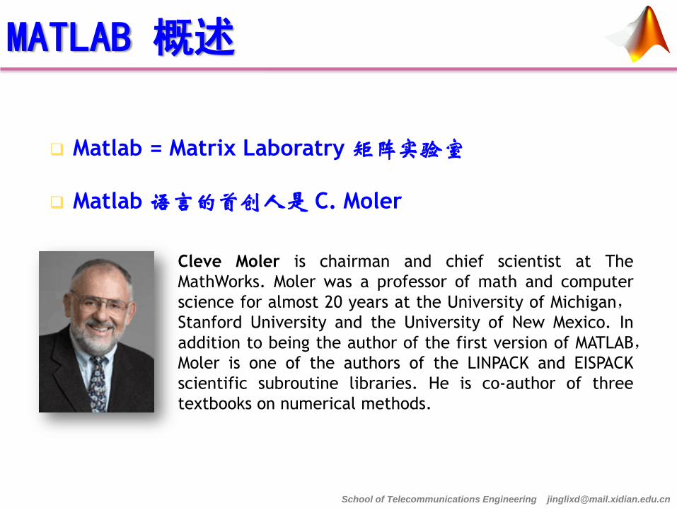
Matlab 语言的首创人是 C. Moler
Matlab = Matrix Laboratry 矩阵实验室
Cleve Moler is chairman and chief scientist at The
MathWorks. Moler was a professor of math and computer
science for almost 20 years at the University of Michigan,
Stanford University and the University of New Mexico. In
addition to being the author of the first version of MATLAB,
Moler is one of the authors of the LINPACK and EISPACK
scientific subroutine libraries. He is co-author of three
textbooks on numerical methods.
MATLAB 概述

School of Telecommunications Engineering [email protected]
70年代中期,Cleve Moler博士和其同事在美国国家科
学基金的资助下开发了调用 EISPACK和 LINPACK的
FORTRAN子程序库.EISPACK是特征值求解的FOETRAN程
序库,LINPACK是解线性方程的程序库.在当时,这两个
程序库代表矩阵运算的最高水平.
70年代后期,Cleve Moler在给学生讲授线性代数课程时,想教学生使用
EISPACK和LINPACK程序库,但他发现学生用FORTRAN编写接口程序很费
时间,于是他开始自己动手,利用业余时间为学生编写EISPACK和
LINPACK的接口程序. Cleve Moler给这个接口程序取名为MATLAB,该名
为矩阵(matrix)和实验室(labotatory)两个英文单词的前三个字母的组合.
在以后的数年里,MATLAB在多所大学里作为教学辅助软件使用,并作为
面向大众的免费软件广为流传.
MATLAB 概述

School of Telecommunications Engineering [email protected]
1983年春天,Cleve Moler到Standford大学讲学,MATLAB深深地吸引了
工程师John Little.
John Little敏锐地觉察到MATLAB在工程领域的广阔前景.同年,他和
Cleve Moler, Steve Bangert一起,用C语言开发了第二代专业版.这一代
的MATLAB语言同时具备了数值计算和数据图示化的功能.
1984年 ,Cleve Moler和John Little成立了Math Works公司 ,正式把
MATLAB推向市场,并继续进行MATLAB的研究和开发.
John Little Cleve Moler
MATLAB 概述

School of Telecommunications Engineering [email protected]
1984年以后又增添了丰富多彩的图形图像处理、多媒体功能、符号运
算和它与其他流行软件的接口功能,使得 Matlab 的功能越来越强大。
到九十年代初期,在国际上 30 几个数学类科技应用软件中, Matlab
在数值计算方面独占鳌头,而 Mathematica 和 Maple 则分居符号计算软
件的前两名。
MATLAB 概述
John Little Cleve Moler
School of Telecommunications Engineering [email protected]
Matlab的发展
1984年,Matlab 1.0版 (DOS版,182K,20来个函数)
1992年,Matlab 4.0版(93年推出Windows版本)
1994年,Matlab 4.2, 1999年, Matlab 5.3
2000年,Matlab 6.0, 2002年, Matlab 6.5
2004年,Matlab 7.0, 2006年, Matlab2006a
2007年,MatlabR2007a
2009年,MatlabR2009a
目前,Matlab 已经成为国际上最流行的科学与工程计算的软件工具,
它已经不仅仅是一个“矩阵实验室”了,而成为了一种具有广泛应用前景
的全新的计算机高级编程语言了,有人称它为“第四代”计算机语言。 就
影响而言,至今仍然没有一个别的计算软件可与 Matlab 匹敌。
MATLAB的发展

School of Telecommunications Engineering [email protected]
数值计算功能
Matlab是一个交互式软件系统
给出一条命令,立即就可以得出该命令的结果
Matlab以矩阵作为基本单位,但无需预先指定维数(动态定维)
按照IEEE的数值计算标准进行计算
提供十分丰富的数值计算函数,方便计算,提高效率
Matlab命令与数学中的符号、公式非常接近,可读性强,容易掌握
符号运算功能
和著名的 Maple 相结合,使得 Matlab 具有强大的符号计算功能
绘图功能
Matlab 提供了丰富的绘图命令,能实现一系列的可视化操作
Matlab的特点与主要功能

School of Telecommunications Engineering [email protected]
编程功能
Matlab 具有程序结构控制、函数调用、数据结构、输入输出、面
向对象等程序语言特征,而且简单易学、编程效率高。
丰富的工具箱(toolbox)
Matlab 包含两部分内容:基本部分和根据专门领域中的特殊需要
而设计的各种可选工具箱。
Simulink 动态仿真集成环境
提供建立系统模型、选择仿真参数和数值算法、启动仿真程序对
该系统进行仿真、设置不同的输出方式来观察仿真结果等功能
PDE
Optimization
Symbolic Math
Signal process
Image Process
Statistics
Control System
System Identification
… …
Matlab的特点与主要功能

School of Telecommunications Engineering [email protected]
把矩阵变为行最简形
求解方程组
计算矩阵的逆
找出向量组的最大无关组
rref 命令

School of Telecommunications Engineering [email protected]
(2)每个台阶只有一行;
(3)台阶数即是非零行的行数,阶梯线的竖线后面的第一个元素为非零元,即非零行的第一个非零元.
特点:
(1)可划出一条阶梯线,线的下方全为零;
4
00000
31000
01110
41211
B
复习:矩阵的行阶梯形和行最简形

School of Telecommunications Engineering [email protected]
(2)每个台阶只有一行;
(3)台阶数即非零行的行数,阶梯线的竖线后面的第一个元素为非零元,即非零行的第一个非零元
特点: (1)可划出一条阶梯线,线的下方全为零;
5
00000
31000
30110
40101
B
(4) 称为最简行阶梯形,即非零行的第一个非零元为1,且这些非零元所在的列的其他元素都为零
5B
复习:矩阵的行阶梯形和行最简形

School of Telecommunications Engineering [email protected]
(1):对调两行(对调i,j 两行,记作 ); (2):以数 乘以某一行的所有元素 (第i行乘以 记作 ); (3):把某一行所有元素的k倍加到另一行对应的元素上去 (第i行的k倍加到第j行上记作: );
同理可定义矩阵的初等列变换(所用记号是把“r”换成“c”).
定义:下面三种变换称为矩阵的初等行变换:
ijr
0 ( )
ir
( )ijr k
复习:矩阵的初等变换

School of Telecommunications Engineering [email protected]
97963
42264
41211
21112
)( bAB
,97963
,42264
,42
,22
4321
4321
4321
4321
xxxx
xxxx
xxxx
xxxx
增
广
矩
阵
系数矩阵
笔算方法:矩阵的初等变换解方程组

School of Telecommunications Engineering [email protected]
1
97963
21132
21112
41211
B
21 rr
23 r
2
34330
63550
02220
41211
B
13
32
2rr
rr
14 3rr
B
笔算方法:矩阵的初等变换解方程组

School of Telecommunications Engineering [email protected]
3
31000
62000
01110
41211
B
23
2
5
2
rr
r
24 3rr 2
B
4
00000
31000
01110
41211
B
43 rr
34 2rr
笔算方法:矩阵的初等变换解方程组

School of Telecommunications Engineering [email protected]
5
00000
31000
30110
40101
B
4B
21 rr
32 rr
对应的方程组为5B
3
3
4
4
32
31
x
xx
xx
笔算方法:矩阵的初等变换解方程组

School of Telecommunications Engineering [email protected]
令 方程组得解可记为: 3x c
3
3
4
4
3
2
1
c
c
c
x
x
x
x
x
3
0
3
4
0
1
1
1
c
笔算方法:矩阵的初等变换解方程组
方程组秩为3, 小于变量个数,方程有无穷多解。
c其中 为任意常数

School of Telecommunications Engineering [email protected]
>> B = [ 2 -1 -1 1 2;1 1 -2 1 4;4 -6 2 -2
4;3 6 -9 7 9]
B =
2 -1 -1 1 2
1 1 -2 1 4
4 -6 2 -2 4
3 6 -9 7 9
5
1 0 1 0 4
0 1 1 0 3
0 0 0 1 3
0 0 0 0 0
B
( )
2 1 1 1 2
1 1 2 1 4
4 6 2 2 4
3 6 9 7 9
B A b
>> B5 = rref(B)
B5 =
1 0 -1 0 4
0 1 -1 0 3
0 0 0 1 -3
0 0 0 0 0
rref 把矩阵变为行最简形并求解方程组
行最简形

School of Telecommunications Engineering [email protected]
rref 命令
把矩阵变为行最简形
求解方程组
计算矩阵的逆
找出向量组的最大无关组
School of Telecommunications Engineering [email protected]
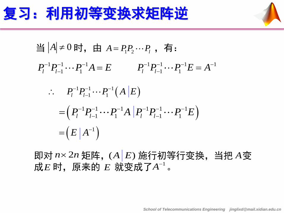
当 时,由 ,有: 0A
1 1 1
1 1l lP P P A E
1 1 1 1
1 1
l lP P P E A
1 1 1 1 1 1
1 1 1 1l l l lP P P A P P P E
1E A
1 1 1
1 1
l lP P P A E
( )A E
复习:利用初等变换求矩阵逆
1 2 lA PP P
即对 矩阵, 施行初等行变换,当把 变 成 时,原来的 就变成了 。
2n n A
E E1A

School of Telecommunications Engineering [email protected]
1A B
E
1 1 ( ) ( )A A B E A B
)( BA
BA1
即
初等行变换
复习:利用初等变换求矩阵逆
利用初等行变换求矩阵逆的办法,还可以用来求矩阵

School of Telecommunications Engineering [email protected]
. ,
343
122
321
1
AA 求设
解
例
103620
012520
001321
100343
010122
001321
EA
12 2rr
13 3rr
笔算方法:利用初等变换求矩阵逆

School of Telecommunications Engineering [email protected]
111100
012520
01120121 rr
23 rr
111100
563020
23100131 2rr
32 5rr
1A)( 22 r
)( 13 r
笔算方法:利用初等变换求矩阵逆
1111002
53
2
3010
231001

School of Telecommunications Engineering [email protected]
>> A = [ 1 2 3; 2 2 1; 3 4 3];
>> B = [ A eye(size(A))]
B =
1 2 3 1 0 0
2 2 1 0 1 0
3 4 3 0 0 1
>> B5 = rref(B)
B5 =
1.0000 0 0 1.0000 3.0000 -2.0000
0 1.0000 0 -1.5000 -3.0000 2.5000
0 0 1.0000 1.0000 1.0000 -1.0000
1 2 3 1 0 0
2 2 1 0 1 0
3 4 3 0 0 1
A E
1
1 0 0 1 3 2
3 50 1 0 3
2 2
0 0 1 1 1 1
E A
rref 求矩阵逆

School of Telecommunications Engineering [email protected]
>> A = [ 1 2 3; 2 2 1; 3 4 3];
>> B5 = inv(A)
B5 =
1.0000 3.0000 -2.0000
-1.5000 -3.0000 2.5000
1.0000 1.0000 -1.0000
inv 命令求矩阵逆
>> A = [ 1 2 3; 2 2 1; 3 4 3];
>> B = [ A eye(size(A))]
B =
1 2 3 1 0 0
2 2 1 0 1 0
3 4 3 0 0 1
>> B5 = rref(B)
B5 =
1.0000 0 0 1.0000 3.0000 -2.0000
0 1.0000 0 -1.5000 -3.0000 2.5000
0 0 1.0000 1.0000 1.0000 -1.0000
使用出错: (奇异,非方阵)
Warning: Matrix is singular to
working precision.
Error using ==> inv
Matrix must be square.

School of Telecommunications Engineering [email protected]
rref 命令
把矩阵变为行最简形
求解方程组
计算矩阵的逆
找出向量组的最大无关组

School of Telecommunications Engineering [email protected]
(1)向量组 线性无关; (2)向量组 中任意 个向量(如果 中有 个向量的 话)都线性相关;
设有向量组 ,如果在 中能选出r个向量 ,满足:
复习:向量组的最大无关组
1 2, , ,
r
0 1 2: , , ,
rA
那么称向量组 是向量组 的一个最大线性无关向量组(简称最大无关组);即:向量组中的其他任一个向量都可以由这 个向量线性表示
A A
A 1r 1r A
0A A
r

School of Telecommunications Engineering [email protected]
复习:向量组的最大无关组
(1)最大无关组不唯一;
(2)向量组与它的最大无关组等价;
(3)一个向量组的任意两个最大无关组等价;
(4)如果向量组本身线性无关,则它是自身的最大线
性无关组;
(5)向量组的极大无关组所含向量的个数称为这个向
量组的秩。

School of Telecommunications Engineering [email protected]
笔算解法:向量组的最大无关组
( ) 3R A
A ,
00000
31000
01110
41211
初等行变换
1 2 4, ,a a a
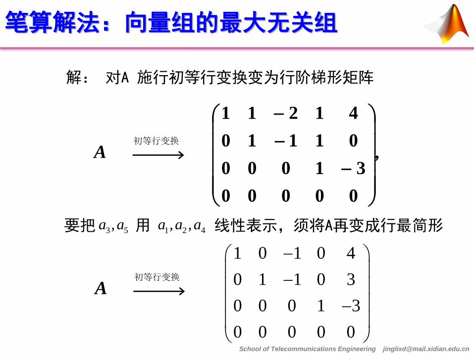
解: 对A 施行初等行变换变为行阶梯形矩阵
故列向量组的最大无关组含三个向量,而三个非
零行的非零首元在1、2、4列,故 为列向量组
的一个最大无关组。
School of Telecommunications Engineering [email protected]
笔算解法:向量组的最大无关组
A ,
00000
31000
01110
41211
解: 对A 施行初等行变换变为行阶梯形矩阵
要把 用 线性表示,须将A再变成行最简形 1 2 4, ,a a a3 5,a a
1 0 1 0 4
0 1 1 0 3
0 0 0 1 3
0 0 0 0 0
初等行变换
A 初等行变换
School of Telecommunications Engineering [email protected]
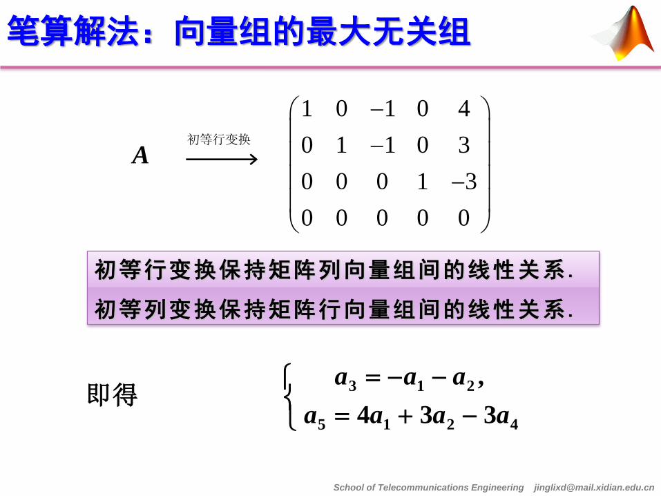
笔算解法:向量组的最大无关组
1 0 1 0 4
0 1 1 0 3
0 0 0 1 3
0 0 0 0 0
4215
213
334
,
aaaa
aaa
即得
初等行变换保持矩阵列向量组间的线性关系.
初等列变换保持矩阵行向量组间的线性关系.
A 初等行变换
School of Telecommunications Engineering [email protected]
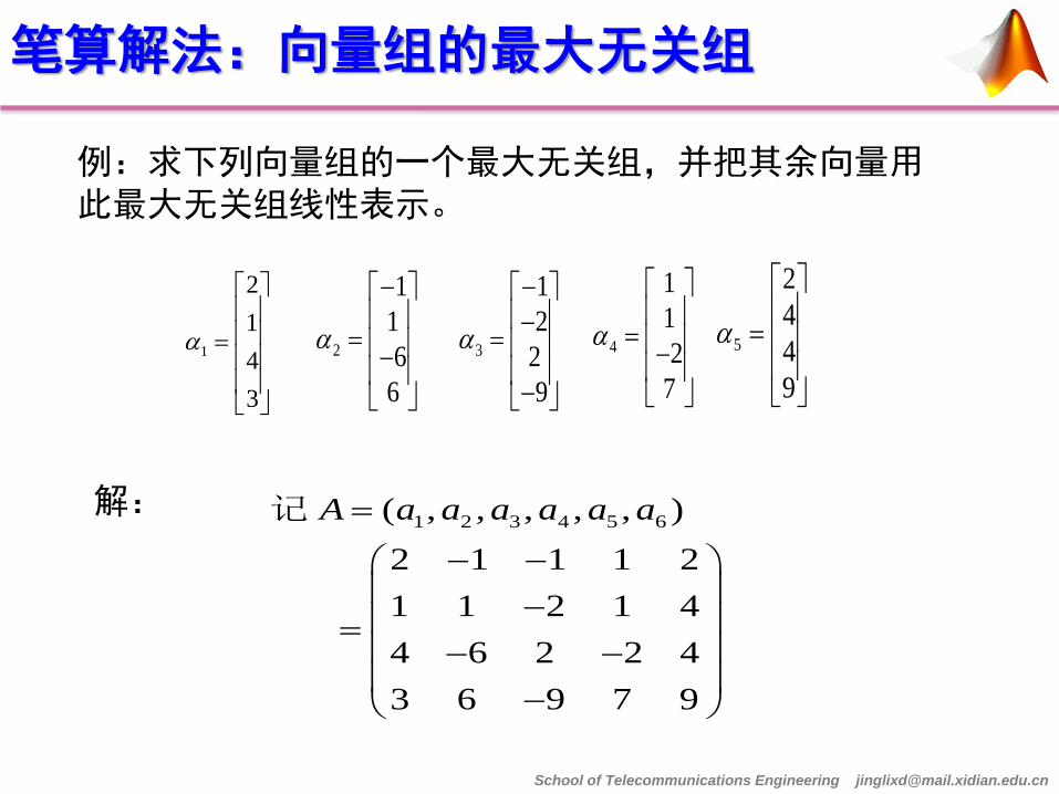
1 2 3 4 5 6 ( , , , , , )
2 1 1 1 2
1 1 2 1 4
4 6 2 2 4
3 6 9 7 9
A a a a a a a
记
2
1
1
6
6
3
1
2
2
9
4
1
1
2
7
5
2
4
4
9
例:求下列向量组的一个最大无关组,并把其余向量用此最大无关组线性表示。
解:
1
2
1
4
3
笔算解法:向量组的最大无关组

School of Telecommunications Engineering [email protected]
直接在MATLAB命令窗口输入以
下命令: % 求向量组的最大无关组
>> clear
>> a1=[2;1;4;3];
>> a2=[-1;1;-6;6];
>> a3=[-1;-2;2;-9];
>> a4=[1;1;-2;7];
>> a5=[2;4;4;9];
>> A=[a1,a2,a3,a4,a5] % 把矩阵A的最简行阶梯矩阵赋给了R
% R的所有基准元素在矩阵中的列号构成了行向量s
>> [R,s]=rref(A)
结果输出为:
A=
2 -1 -1 1 2
1 1 -2 1 4
4 -6 2 -2 4
3 6 -9 7 9
R =
1 0 -1 0 4
0 1 -1 0 3
0 0 0 1 -3
0 0 0 0 0
s =
1 2 4
rref 命令求解向量组的最大无关组
School of Telecommunications Engineering [email protected]
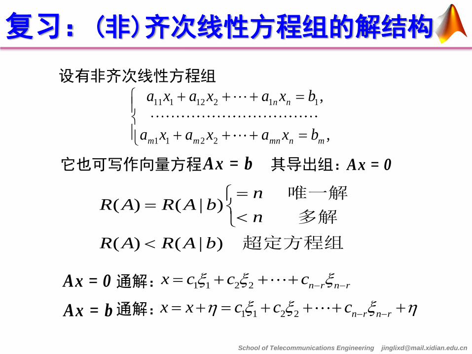
设有非齐次线性方程组
11 1 12 2 1 1
1 1 2 2
,
,
n n
m m mn n m
a x a x a x b
a x a x a x b
它也可写作向量方程 Ax = b Ax = 0其导出组:
复习:(非)齐次线性方程组的解结构
1 1 2 2 n r n rx c c c
通解:
1 1 2 2 n r n rx x c c c
通解:
( ) ( | )
( ) ( | )
nR A R A b
n
R A R A b
唯一解
多解
超定方程组
Ax = b
Ax = 0

School of Telecommunications Engineering [email protected]
1 2 5
1 2 3
3 4 5
2
3
5
x x x
x x x
x x x
笔算解法:非齐次线性方程组的解
例:求非齐次线性方程组的基础解系和通解
1 1 0 0 1 2 1 1 0 0 1 2
( | ) 1 1 1 0 0 3 0 0 1 0 1 1
0 0 1 1 1 5 0 0 0 1 0 6
1 1 0 0 1 2
0 0 1 0 1 1
0 0 0 1 0 6
A b
解:对增广矩阵作初等变换,化为行最简形有:
( ) ( | ) 3R A R A b n

School of Telecommunications Engineering [email protected]
1 21, 1, 0, 0, 0 , 1, 0, 1, 0, 1 ,T T
-
笔算解法:非齐次线性方程组的解
其中 自由变量 令: 5, ( ) 3,n R A
2n r
2
5
1 0,
0 1
x
x
和
2,n r
1 1 2 2x k k 导出组的通解为:
导出组对应的基础解系是 个解向量:
1 2 5
3 5
4
2
1,
6
x x x
x x
x
得同解方程组为:
2, 0, 1, 6, 0T
非齐次线性方程组的通解为:
1 1 2 2x k k
School of Telecommunications Engineering [email protected]
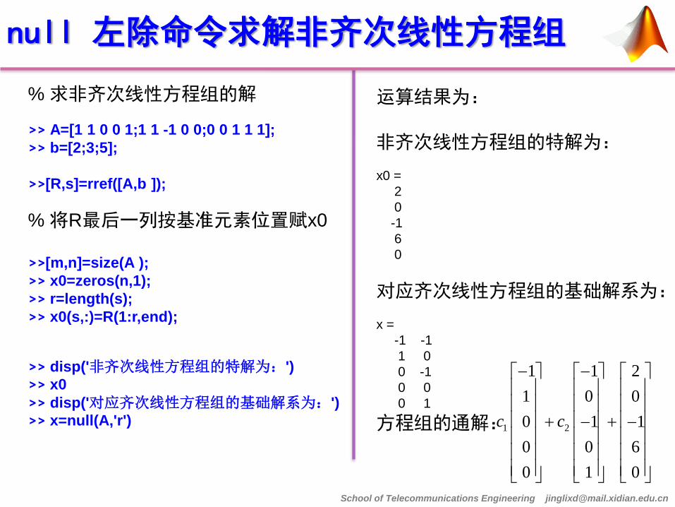
% 求非齐次线性方程组的解
>> A=[1 1 0 0 1;1 1 -1 0 0;0 0 1 1 1];
>> b=[2;3;5];
>>[R,s]=rref([A,b ]);
% 将R最后一列按基准元素位置赋x0
>>[m,n]=size(A );
>> x0=zeros(n,1);
>> r=length(s);
>> x0(s,:)=R(1:r,end);
>> disp('非齐次线性方程组的特解为:')
>> x0
>> disp('对应齐次线性方程组的基础解系为:')
>> x=null(A,'r')
null 左除命令求解非齐次线性方程组
运算结果为: 非齐次线性方程组的特解为:
x0 =
2
0
-1
6
0
对应齐次线性方程组的基础解系为:
x =
-1 -1
1 0
0 -1
0 0
0 1
方程组的通解:
1 2
1 1 2
1 0 0
0 1 1
0 0 6
0 1 0
c c

School of Telecommunications Engineering [email protected]
非齐次线性方程组的特解还可以用MATLAB的矩阵左除运算来求得,直接在MATLAB命令窗口输入以下命令:
clear
>> A=[1 1 0 0 1;1 1 -1 0 0;0 0 1 1 1];
>> b=[2;3;5];
[R,s]=rref([A,b ]);
>> x0=A\b;
>> disp('非齐次线性方程组的特解为:')
>> x0
>> disp('对应齐次线性方程组的基础解系为:')
>> x=null(A,'r')
其中特解x0与前一方法的特解不同。 (注:如果欠定方程组有解,则它有无穷个特解,通解中只需要任何一个特解即可)
null 左除命令求解非齐次线性方程组
运算结果为: 非齐次线性方程组的特解为:
x0 =
3.0000
0
0
6.0000
-1.0000
对应齐次线性方程组的基础解系为:
x =
-1 -1
1 0
0 -1
0 0
0 1
方程组的通解: 1 2
1 1 3
1 0 0
0 1 0
0 0 6
0 1 1
c c

School of Telecommunications Engineering [email protected]
复习:向量组的正交规范化
向量的内积(inner product)
设有n维向量 ,称数
为向量 与 的内积,记作
1 2 1 2, , , , , , ,T T
n na a a b b b
1 1 2 2 n na b a b a b ,
1 1 2 2, T
n na b a b a b
零向量与任何向量正交。
不含零向量的两两正交的向量组称为正交向量组
正交向量组是线性无关的
向量的夹角
如果 ,令 ,则称 为向量 与 的夹角。
,0 0 ,
arccos ,0
当 时,夹角 ,称向量 与 正交。 2
, 0

School of Telecommunications Engineering [email protected]
复习:向量组的正交规范化
正交向量组是线性无关的
施密特(Schimidt)正交化方法
1 1 2 1
2 2 1
1 1
,
,
如果向量组 线性无关,则下列方法得到的
向量组 是正交组,且与向量组 等价。
1 2, , , r
1 2, , , r 1 2, , , r
1 2 1
1 2 1
1 1 2 2 1 1
1
1
, , ,
, , ,
,
,
r r r r
r r r
r r
rr j
r j
j j j
1 2, , , re e e
单位化得到规范正交组:

School of Telecommunications Engineering [email protected]
笔算解法:向量组的正交规范化
例:将向量组正交规范化
1 2 31,2, 1 , 1,3,1 , 4, 1,0T T T
解:令 1 1 1,2, 1T
3 1 3 2
3 3 1 2
1 1 2 2
, ,
, ,
4 1 1 11 5
1 2 1 2 03 3
0 1 1 1
2 1
2 2 1
1 1
1 1 1, 4 5
3 2 1, 6 3
1 1 1

School of Telecommunications Engineering [email protected]
笔算解法:向量组的正交规范化
11
1
11
26
1
e
33
3
11
02
1
e
将 单位化,得 1 2 3, ,
则 为所求的规范正交组。 1 2 3, ,e e e
22
2
11
13
1
e

School of Telecommunications Engineering [email protected]
在MATLAB命令窗口输入以下命令:
clear
>> a1=[1 2 -1]' ;
>> a2=[-1,3,1]';
>> a3=[4 -1 0]';
>> A =[a1 a2 a3];
>> B =orth(A)
orth 命令求解规范正交组
运算结果为: B = 0.8245 0.5548 0.1112 -0.5546 0.8313 -0.0357 -0.1122 -0.0323 0.9932

School of Telecommunications Engineering [email protected]
复习:矩阵的特征值和特征向量
工程实践中有多种振动问题,如桥梁或建筑物的振动,机械机件、飞机机翼的振动,及一些稳定性分析和相关分析可转化为求矩阵特征值与特征向量的问题。
定义:设 是 阶矩阵,如果数 和 维非零列向
量 使关系式:
成立,那么数 成为方程 的特征值,非零向量 称为
的对应于特征值 的特征向量。
A
x
n n
Ax x
A x A

School of Telecommunications Engineering [email protected]
1、特征向量 ,特征值问题是对方阵而言的。
2、 阶方阵 的特征值,就是使齐次线性方程组
有非零解的 值,其满足方程
的 都是矩阵A的特征值。
复习:矩阵的特征值和特征向量
0x
n A
( ) 0A E x
| | 0A E

School of Telecommunications Engineering [email protected]
笔算方法:矩阵特征值和特征向量
例 设 ,
314
020
112
A 求A的特征值与特征向量.
解
314
020
112
EA 2
( 1) 2
02)1(2 令
.2,1 321 的特征值为得A

School of Telecommunications Engineering [email protected]
笔算方法:矩阵特征值和特征向量
由解方程时当 .0,11 xEA
1 1 1 1 0 1
0 3 0 0 1 0 ,
4 1 4 0 0 0
A E
,
1
0
1
1
p得基础解系
的全体特征向量为故对应于 11
).0( 1
kpk
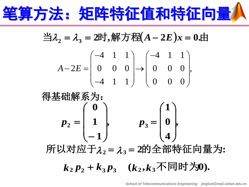
School of Telecommunications Engineering [email protected]
笔算方法:矩阵特征值和特征向量
由解方程时当 .02,232 xEA
4 1 1 4 1 1
2 0 0 0 0 0 0 ,
4 1 1 0 0 0
A E
得基础解系为:
,
4
0
1
,
1
1
0
32
pp
:232 的全部特征向量为所以对应于
).0,( 323322 不同时为kk pkpk

School of Telecommunications Engineering [email protected]
机算方法:矩阵特征值和特征向量
在MATLAB命令窗口输入以下命令:
>> A =[-2 1 1; 0 2 0;-4 1 3];
>> [p,lamda] =eig(A)
运算结果为: p = -0.7071 -0.2425 0.3015 0 0 0.9045 -0.7071 -0.9701 0.3015 lamda = -1 0 0 0 2 0 0 0 2
School of Telecommunications Engineering [email protected]
复习:二次型的标准化及正定判别
nnnn
nnnn
xxaxxaxxa
xaxaxaxxxf
1,131132112
22
222
2
11121
222
,,,
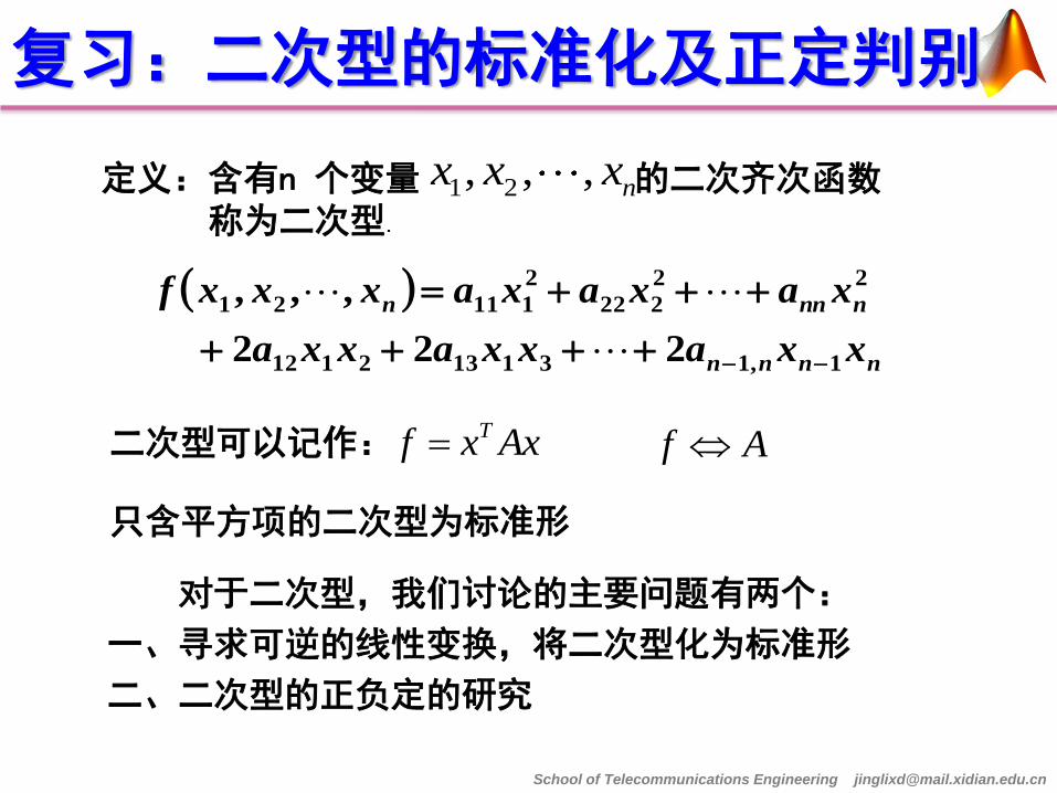
定义:含有n 个变量 的二次齐次函数 称为二次型.
1 2, , , nx x x
Tf x Ax二次型可以记作:
只含平方项的二次型为标准形
f A
对于二次型,我们讨论的主要问题有两个:
一、寻求可逆的线性变换,将二次型化为标准形
二、二次型的正负定的研究

School of Telecommunications Engineering [email protected]
复习:二次型的标准化及正定判别
二次型标准化主要有三种方法:正交变换化,拉格朗日 配方法和初等变换法。
对于实二次型 ,如果对于任意 都有 则称 为正定二次型,对应的矩阵为正定矩阵;如果对任意 都有 ,则称 为负定二次型,对应的矩阵为负 定矩阵。
Tf x Ax f ( ) 0f x f
f ( ) 0f x f
判别二次型正定主要有三种方法:定义法,矩阵特征值法, 顺序主子式判别方法(霍尔维茨定理)。

School of Telecommunications Engineering [email protected]
笔算方法:二次型的标准化及正定判别
例: 用正交变换将二次型标准化,并求其变换矩阵
xzxyzyxf 44465 222
解:用正交变换化二次型为标准形的具体步骤:
;,.1 AAxxf T 求出将二次型表成矩阵形式
;,,,.2 21 nA 的所有特征值求出
;,,,.3 21 n 征向量求出对应于特征值的特
;,,,,,,,
,,,,,.4
2121
21
nn
n
C
记
得单位化正交化将特征向量
.
,.5
22
11 nn yyf
fCyx
的标准形则得作正交变换

School of Telecommunications Engineering [email protected]
笔算方法:二次型的标准化及正定判别
例: 用正交变换将二次型标准化,并求其变换矩阵
解法: 1、对称矩阵为:
2 2 2
1 2 3 1 2 1 3 2 3 17 14 14 4 4 8f x x x x x x x x x
1442
4142
2217
A
1442
4142
2217
EA 9182
2、求特征值:
School of Telecommunications Engineering [email protected]
笔算方法:二次型的标准化及正定判别
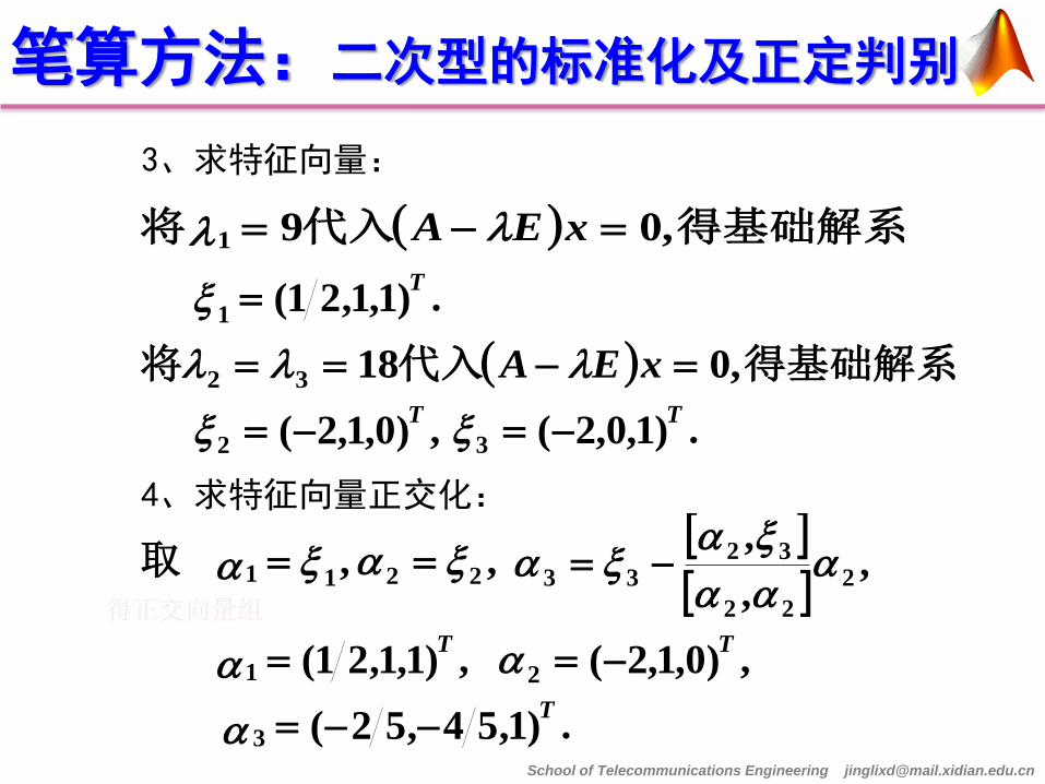
得基础解系代入将 ,091 xEA
得基础解系代入将 ,01832 xEA
,)0,1,2(2 T
.)1,0,2(3 T
.)1,1,21(1
T
3、求特征向量:
,11 取 ,22
,,
,2
22
3233
得正交向量组
.)1,54,52(3 T
,)0,1,2(2 T
,)1,1,21(1
T
4、求特征向量正交化:

School of Telecommunications Engineering [email protected]
笔算方法:二次型的标准化及正定判别
,3,2,1, ii
ii
令
,
0
51
52
2
,
32
32
31
1
.
455
454
452
3
4.将正交向量组单位化,得正交矩阵 P
于是所求正交变换为:
,
455032
4545132
4525231
3
2
1
3
2
1
y
y
y
x
x
x
.181892
3
2
2
2
1 yyyf 且有

School of Telecommunications Engineering [email protected]
笔算方法:二次型的标准化及正定判别
例: 判定二次型正定性
解法一: 二次型的矩阵为
11 17 0,a 11 12
21 22
17 2234 0,
2 14
a a
a a
2916 0,A
根据霍尔维茨定理该二次型的矩阵为正定矩阵。
2 2 2
1 2 3 1 2 1 3 2 3 17 14 14 4 4 8f x x x x x x x x x
1442
4142
2217
A

School of Telecommunications Engineering [email protected]
笔算方法:二次型的标准化及正定判别
例: 判别二次型的正定性
解法二:
特征值都大于零,因此可以判别该二次型的矩阵为正定矩阵。
0 AE令1 2 39, 18, 18.
特征值判别法
二次型的矩阵为
2 2 2
1 2 3 1 2 1 3 2 3 17 14 14 4 4 8f x x x x x x x x x
1442
4142
2217
A

School of Telecommunications Engineering [email protected]
在MATLAB命令窗口输入以下命令:
>> A=[17 -2 -2;-2 14 -4; -2 -4 14]
>> disp('矩阵特征值和特征向量为:')
>> [P,lamda] = eig(A)
>> disp('顺序主子式为:')
for i=1:size(A,1)
det(A(1:i,1:i))
end
eig 二次型标准化及正定判别
运算结果为: 矩阵特征值和特征向量为: P = 0.3333 -0.2981 0.8944 0.6667 -0.5963 -0.4472 0.6667 0.7454 0.0000 lamda = 9 0 0 0 18 0 0 0 18 顺序主子式为: ans = 17 ans = 234 ans = 2916 可判定矩阵为正定矩阵。
1442
4142
2217
A

School of Telecommunications Engineering [email protected]
(1)图像的代数操作
1. 相加运算 2. 减法运算 3. 乘法运算 4. 除法运算
代数操作是指对图像进行点对点的加、减、乘、除四则运算而得到一幅新的输出图像, 参与运算的像素几何位置不变。 记输入图像为A(x,y)和B(x,y),输出图像为C(x,y),则图像代数操作有如下四种简单形式:
C(x,y) = A(x,y)+B(x,y)
C(x,y) = A(x,y)—B(x,y)
C(x,y) = A(x,y)×B(x,y)
C(x,y) = A(x,y)/ B(x,y)
矩阵的基本运算

School of Telecommunications Engineering [email protected]
(1)图像的代数操作——相加运算
图像相加常用于图像合成,以及对同一场景的多幅图像求平均,有效地降低加性随机噪声。
= +

School of Telecommunications Engineering [email protected]
% ImAdd.m
% 读入图像
ima1 = imread('vase.jpg');
ima2 = imread('sky.jpg');
% 转换数据类型
ima1 = double(ima1);
ima2 = double(ima2);
% 加法求平均
result = (ima1+ima2)/2;
figure; imshow(uint8(result));
= + vase.jpg
sky.jpg
result
(1)图像的代数操作——相加运算

School of Telecommunications Engineering [email protected]
图像相加常用于对同一场景的多幅图象求平均,以便有效地降低加性随机噪声,通常对于经过长距离模拟通讯方式传送的图像,这种处理是不可缺少的。
(1)图像的代数操作——相加运算

School of Telecommunications Engineering [email protected]
= —
图像相减是常用的图像处理方法,用于检测图像变化及运动物体。
(1)图像的代数操作——相减运算

School of Telecommunications Engineering [email protected]
图像相减是常用的图像处理方法,用于检测图像变化及运动物体。
(1)图像的代数操作——相减运算

School of Telecommunications Engineering [email protected]
(2)图像的几何变换
图像的几何变换操作会改变图像中(像素)之间的空间关系,这种运算可以看成是图像内的各像素在图像内移动的过程。 典型的几何变换包括:平移、旋转、缩放、相似变换、仿射变换、非线性变换等。

School of Telecommunications Engineering [email protected]
(2)图像的几何变换——平移
0' xxx
1100
10
01
1
'
'
0
0
y
x
y
x
y
x
0' yyy

School of Telecommunications Engineering [email protected]
(2)图像的几何变换——旋转
)cos()sin('
)sin()cos('
yxy
yxx
1100
0)cos()sin(
0)sin()cos(
1
'
'
y
x
y
x

School of Telecommunications Engineering [email protected]
(2)图像的几何变换——缩放
' 0 0
' 0 0
1 0 0 1 1
x sx x
y sy y

School of Telecommunications Engineering [email protected]
(2)图像的几何变换——非线性变换
图像卷绕是通过指定一系列控制点的位移来定义空间变换的图象变形处理。非控制点的位移根据控制点进行插值来确定。

School of Telecommunications Engineering [email protected]
图像变形是使图像中的一个物体逐渐变形为另外一个物体的过程。从一起始图像出发,利用渐隐(dissolve)技术,使起始图象逐渐“淡出(fade out)”,而目标图像则逐渐“淡入(fade in)”,同时以对应物体为转换控制对象,通过选择控制点及控制线来建立插值过程,让物体上的点从它们的起始位置逐渐移向对应的终止位置。
(2)图像的几何变换——非线性变换

School of Telecommunications Engineering [email protected]
(3)图像配准
图像配准是评价两幅或多幅图像的相似性以确定同名点的过程。
图像配准算法就是设法建立两幅图像之间的对应关系,确定相应几何
变换参数,对两幅图像中的一幅进行几何变换的方法。
图像配准是图像分析和处理的基本问题。它在遥感测绘、图像导航、
目标识别、视频数据检索、医学影像处理、视频监控、生物特征识别、
纹理分析、三维重构、虚拟现实与增强现实等领域都有重要应用。

School of Telecommunications Engineering [email protected]
(3)图像配准
图像配准的主要步骤
对特征进行描述和匹配
根据对应点估计空间变换关系
对图像进行逐像素处理变为配准图
独立的寻找出具有相同内容的图像特征区域
特征
描述与匹配
变换模型
参数估计 几何校正 特征检测
School of Telecommunications Engineering [email protected]
(3)图像配准
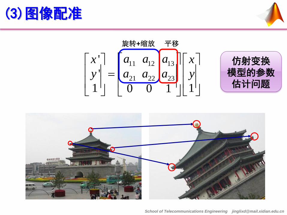
11 12 13
21 22 23
'
'
1 10 0 1
a a ax x
y a a a y
旋转+缩放 平移
仿射变换 模型的参数估计问题
School of Telecommunications Engineering [email protected]
(3)图像配准
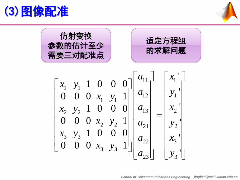
仿射变换 参数的估计至少需要三对配准点
适定方程组 的求解问题
11 1
1 1
12 11 1
13 22 2
2 2 221
3 3322
3 3
23 3
'1 0 0 0
'0 0 0 1'1 0 0 0
0 0 0 1 '1 0 0 0 '
0 0 0 1'
a xx y
a yx ya xx y
x y yax y xa
x ya y

School of Telecommunications Engineering [email protected]
(3)图像配准
Matched Points Number:86
11 12 13
21 22 23
'
'
1 10 0 1
a a ax x
y a a a y
旋转+缩放 平移
仿射变换 模型的参数估计问题

School of Telecommunications Engineering [email protected]
(3)图像配准
11
11 1
121 1
1
13
21
22
23
'1 0 0 0
0 0 0 1 '... ... .... ... ... ...
'1 0 0 0
'0 0 0 1
nn n
nn n
axx y
ax y y
a
axx y
ayx y
a
AX b
1( )T TX A A A b
多对配准点 对仿射变换 参数的估计
超定方程组 的求解问题

School of Telecommunications Engineering [email protected]
(3)图像配准
全景图自动拼接 http://www.cs.ubc.ca/~mbrown/autostitch/autostitch.html

School of Telecommunications Engineering [email protected]
(4)综合示例——无人机航拍视频内容分析 http://server.cs.ucf.edu/~vision/projects/COCOAWebsite/CocoaWebsite/featured_project.html