Dissipation in Turbulent · PDF fileturbulence textbooks and research activity over the past seven decades is indeed the Richardson-Kolmogorov cascade. Rigid boundaries also introduce

FL47CH05-Vassilicos ARI 2 December 2014 12:14

Dissipation in Turbulent FlowsJ. Christos VassilicosDepartment of Aeronautics, Imperial College London, London SW7 2AZ, United Kingdom;email: [email protected]

Annu. Rev. Fluid Mech. 2015. 47:95–114

First published online as a Review in Advance onAugust 25, 2014

The Annual Review of Fluid Mechanics is online atfluid.annualreviews.org

This article’s doi:10.1146/annurev-fluid-010814-014637

Copyright c© 2015 by Annual Reviews.All rights reserved

Keywords

Richardson-Kolmogorov cascade, nonequilibrium turbulence, turbulencedissipation scalings

Abstract

This article reviews evidence concerning the cornerstone dissipation scalingof turbulence theory: ε = CεU3/L, with Cε = const., ε the dissipation rateof turbulent kinetic energy U2, and L an integral length scale characterizingthe energy-containing turbulent eddies. This scaling is intimately linked tothe Richardson-Kolmogorov equilibrium cascade. Accumulating evidenceshows that a significant nonequilibrium region exists in various turbulentflows in which the energy spectrum has Kolmogorov’s −5/3 wave-numberscaling over a wide wave-number range, yet Cε ∼ Rem

I /RenL, with m ≈ 1 ≈ n,

Re I a global/inlet Reynolds number, and ReL a local turbulence Reynoldsnumber.

95

Ann

u. R

ev. F

luid

Mec

h. 2

015.

47:9

5-11

4. D

ownl

oade

d fr

om w

ww

.ann

ualr

evie

ws.

org

Acc

ess

prov

ided

by

Impe

rial

Col

lege

Lon

don

on 0

5/29

/15.

For

per

sona

l use

onl

y.


1. INTRODUCTION

This review begins with quotations from two influential textbooks and one APS Fluid DynamicsPrize presentation. Referring to the well-known estimate ε ∼ U3/L (where ε is the dissipationrate of turbulent kinetic energy U2, and L is the integral length scale), Tennekes & Lumley (1972)stated that this estimate “should not be passed over lightly. It is one of the cornerstone assumptionsof turbulence theory.” In a paper that Lumley (1992) wrote 20 years later on the occasion of hisaward of the APS Fluid Dynamics Prize, he included the following question and answer: “Whatpart of modeling is in serious need of work? Foremost, I would say, is the mechanism that sets thelevel of dissipation in a turbulent flow, particularly in changing circumstances.” And in one of themore recent and most widely used textbooks on turbulence, Pope’s (2000) chapter “The Scales ofTurbulent Motion” begins with a brief description of the Richardson-Kolmogorov cascade thatends “this picture of the cascade indicates that ε scales as U3/L independent of ν (at the highReynolds numbers being considered),” where ν is the fluid’s kinematic viscosity.

The one mechanism for turbulence dissipation at high Reynolds numbers that has dominatedturbulence textbooks and research activity over the past seven decades is indeed the Richardson-Kolmogorov cascade. Rigid boundaries also introduce their own dissipation mechanism in thecase of turbulent flows attached to or affected by a wall. However, the Richardson-Kolmogorovcascade is present (or at least believed to be present) far enough from the wall in many suchflows, as in boundary-free turbulent flows, and this review therefore concentrates on the pervasiveturbulence dissipation mechanism caused by this cascade. Section 2 briefly reviews this mechanismand its consequences, and Section 3 follows with a review of the experimental evidence gatheredin support of ε ∼ U3/L in the 50 years after Kolmogorov (1941a,b,c). Section 4 discusses theexperimental and computational support for ε ∼ U3/L in the past 25 years, and Section 5 reviewsthe support gathered for a different scaling relation in the past 8 years. Section 6 concludes witha summary and discussion of the new perspectives now opening for research in turbulent flows.

2. THE RICHARDSON-KOLMOGOROV CASCADE

The Richardson-Kolmogorov cascade is a mechanism for turbulence dissipation at high Reynoldsnumbers when the turbulence is assumed to be at equilibrium (see the chapter “The UniversalEquilibrium Theory” in Batchelor 1953; note that the word equilibrium in this chapter and in thepresent review is not used in the sense reserved in statistical physics for stationary states satisfyingdetailed balance such as thermal equilibria). The kinetic energy of velocity fluctuations cascadesfrom large to small scales of motion. When it reaches a scale small enough for viscous dissipationto be effective, it dissipates into heat (see Richardson 1922). This cascade is an equilibrium cascade.The rate at which kinetic energy crosses a length scale r where the turbulent fluctuations havea characteristic velocity u(r) is the same from the largest to the smallest length scale r in theappropriate range of scales. This rate can be dimensionally estimated as u(r)3/r (no viscosity) andcan be equated (equilibrium) to the turbulent kinetic energy dissipation ε = ν <s2>, where sis the fluctuating turbulence strain rate tensor, and the brackets signify an appropriate averagingoperation. The largest such length scale r is of the order of the integral length scale L so thatu(r) = u(L) ∼ U . Hence, it follows that ε ∼ U3/L.

These words translate into equations in a way that is based on a relatively recent generalizationand use of the Karman-Howarth equation that is worth recording in this review. Defining δu ≡u(x + 1

2 r, t) − u(x − 12 r, t), where u is the fluctuating velocity field at a given point in space and

time, one takes the mathematical definition of u(r) to be√

<|δu|2>, which is a function of x andr. The brackets are an average over time or over statistical realizations of the turbulence. The

96 Vassilicos

Ann

u. R

ev. F

luid

Mec

h. 2

015.

47:9

5-11

4. D

ownl

oade

d fr

om w

ww

.ann

ualr

evie

ws.

org

Acc

ess

prov

ided

by

Impe

rial

Col

lege

Lon

don

on 0

5/29

/15.

For

per

sona

l use

onl

y.


Navier-Stokes equation and incompressibility at both ξ = ξ+ ≡ x + 12 r and ξ = ξ+ ≡ x − 1

2 r are

∂

∂t(U + u) + (U + u) · ∇ξ (U + u) = −∇ξ (P + p) + ν∇2

ξ (U + u) (1)

and ∇ξ ·U = 0, ∇ξ ·u = 0, where U is the mean flow field and the Reynolds decomposition U + u isused. From these equations written at both points ξ = ξ+ and ξ = ξ−, Hill (2002) and Marati et al.(2004), followed by Danaila et al. (2012) and P. Valente & J.C. Vassilicos (submitted manuscript),derived the generalized Karman-Howarth equation, which is valid with no homogeneity and noisotropy assumptions:

D∗

Dt<|δu|2> + ∇r <(δu + δU)|δu|2> = P∗ + T ∗ + D∗ + ν∇2

r <|δu|2> −4ε∗, (2)

where D∗/(Dt) ≡ ∂/(∂t) + 12 [U(ξ+) + U(ξ−)] · ∇x , and P∗, T∗, and D∗ are terms that result from

the turbulence production by the mean flow and Reynolds stresses, turbulent transport in termsof gradients in x space of correlations between velocity fluctuations and both energy and pressurefluctuations, and viscous diffusion in x space, respectively. The penultimate term on the right-hand side represents viscous diffusion in r space, and the two-point dissipation term ε∗ equals12 (ε(ξ+) + ε(ξ−)).

At high-enough Reynolds numbers, the two-point viscous diffusion term D∗ may be neglected.If we consider regions of turbulent flows where the integral scale L of the turbulent fluctuatingvelocity is smaller than or comparable to length scales characterizing spatial variations in x ofmean flow statistics, then for high Reynolds numbers and r < L,

∂

∂t<|δu|2> + U(x) · ∇x <|δu|2> + ∇r· <δu|δu|2> = ν∇2

r <|δu|2> −4ε. (3)

Laizet et al. (2013) and P. Valente & J.C. Vassilicos (submitted manuscript) obtained a sufficientcondition for the diffusion term ν∇2

r <|δu|2> to be negligible compared to 4ε and therefore dropout so as to be left with

∂

∂t<|δu|2> + U(x) · ∇x <|δu|2> + ∇r· <δu|δu|2> = −4ε. (4)

This sufficient condition is r � λ, where λ2 ≡ νU2/ε (i.e., λ is effectively the Taylor microscale).In small-scale isotropic turbulence, Goto & Vassilicos (2009) proved under mild assumptions thatλ is proportional to the average distance between stagnation points of the fluctuating velocityfield. Hence, the fluctuating velocity is much rougher at scales larger than λ than at scales smallerthan λ. Equation 4 therefore describes the rough range of the locally homogeneous velocity field,that is, the range of length scales r between λ (for roughness) and L (for local homogeneity in theappropriate conditions).

The key equilibrium assumption made by Kolmogorov (1941b) is that the small-scale motions(r � L) evolve very quickly compared to the timescale of the overall turbulence evolution and aretherefore in statistical equilibrium [i.e., ∂/(∂t) <|δu|2> + U(x) ·∇x <|δu|2> ≈ 0]. The equilibriumcascade then follows in the form ∇r· <δu|δu|2> ≈ −4ε. Nie & Tanveer (1999) (see also Duchon& Robert 2000, Eyink 2003) introduced the procedure of integrating both sides over a sphere ofradius |r| = r , which, using the Gauss divergence theorem, yields∫

r· <δu|δu|2> d� ≈ −16π

3εr, (5)

where d� is the differential of the solid angle in r space and r ≡ r/r .This may be seen as summarizing the modern mathematical treatment and resulting expres-

sion of the Richardson-Kolmogorov cascade for equilibrium turbulence. The spherically averaged

www.annualreviews.org • Dissipation in Turbulent Flows 97

Ann

u. R

ev. F

luid

Mec

h. 2

015.

47:9

5-11

4. D

ownl

oade

d fr

om w

ww

.ann

ualr

evie

ws.

org

Acc

ess

prov

ided

by

Impe

rial

Col

lege

Lon

don

on 0

5/29

/15.

For

per

sona

l use

onl

y.


interscale energy flux in physical space is negative, which means that the cascade is from largeto small scales because turbulence velocity differences are being compressed (i.e., transported tosmaller scales). The self-similarity of the cascade is also evident in this expression as the rate ofenergy across scales is determined by ε, regardless of the scale r in the appropriate range. Thisself-similarity is the basis for the dimensional analysis leading to the celebrated E(k) ∼ ε2k−5/3 scal-ing of the turbulence energy spectrum E(k) (e.g., see Pope 2000). Finally, to quote Pope (2000),this mathematical expression “of the cascade indicates that ε scales as U3/L independent of ν

(at the high Reynolds numbers being considered).” Indeed, for r ∼ L, one expects∫r· <δu|δu|2> d� ∼ U3, which, from Equation 5, implies the equilibrium dissipation law

ε = CεU3/L, (6)

with Cε = const. independent of the Reynolds number at high-enough Reynolds numbers.The clear weakness of this derivation is that Equation 5 holds for r � L, yet Equation 5 isused for r ∼ L. These two conditions on r are not necessarily incompatible if one can write∫

l· <δu|δu|2> d� ∼ U3 for a scale smaller than L that is nevertheless a fixed fraction of L.Equation 6 and λ2 ≡ νU2/ε imply that

L/λ ∼ Cε Reλ, (7)

where Reλ ≡ (Uλ)/ν is a local Reynolds number dependent on the position in the flow as U and λ

depend on x. This relation demonstrates that L � λ if Reλ � 1 and therefore that intermediatescales r at which λ � r � L do exist at high-enough Reynolds numbers. In fact, Equation 7expresses a central idea of the Richardson-Kolmogorov cascade: the higher the Reynolds number,the higher the range of scales required for the turbulent energy to be dissipated. This followsfrom the Richardson-Kolmogorov cascade’s indication (to use Pope’s word) that Cε = const.Below are a few facts that substantiate Tennekes & Lumley’s (1972) statement that the dissipationrelation given in Equation 6 with Cε = const. “should not be passed over lightly. It is one of thecornerstone assumptions of turbulence theory.” It is noted that Equation 6 with Cε = const. isan assumption for Tennekes & Lumley (1972), and also for Frisch (1995) (see below), whereasKolmogorov (1941a,b) saw it as a consequence of his equilibrium assumption. Either way, thereis a cornerstone assumption here that should not be passed over lightly.

First, the turbulent eddy viscosity νt in one-point Reynolds-averaged Navier-Stokes models ofturbulence (see Launder & Spalding 1972, Pope 2000) is estimated using νt ∼ UL and Equation 6with Cε = const. : νt ∼ CεU4/ε. Second, two-point turbulence modeling such as large-eddy simu-lations (see Lesieur & Metais 1996, Meneveau & Katz 2000) relies on the Richardson-Kolmogorovequilibrium cascade, which indicates that Equation 6 holds with Cε = const. Third, the numberof degrees of freedom is usually estimated as (L/η)3, where η = (ν3/ε)1/4 is the Kolmogorov mi-croscale. The equilibrium relation given in Equation 6 with Cε = const. is crucial in determiningthat (L/η)3 ∼ Re9/4

L ; ReL is another local Reynolds number based on U and L, both of which aredependent on x. Relations such as (L/η)3 ∼ C3/4

ε Re9/4L are pivotal when choosing the resolution

of computer simulations of turbulent flows. Finally, the equilibrium dissipation relation given inEquation 6 with Cε = const. effectively determines the streamwise development of mean profilesof self-preserving turbulent free shear flows (Townsend 1976, George 1989).

3. EVIDENCE FOR ε ∼ U3/L IN THE 50 YEARS AFTER THE 1941PAPERS OF KOLMOGOROV

The equilibrium dissipation law in Equation 6 with Cε = const. was in fact first introducedby Taylor (1935) without much justification six years before Kolmogorov’s 1941 papers.

98 Vassilicos

Ann

u. R

ev. F

luid

Mec

h. 2

015.

47:9

5-11

4. D

ownl

oade

d fr

om w

ww

.ann

ualr

evie

ws.

org

Acc

ess

prov

ided

by

Impe

rial

Col

lege

Lon

don

on 0

5/29

/15.

For

per

sona

l use

onl

y.


1.0

2.0

3.0

8 6 4 2 0 2 4 6 8

Injection rate (%)

COUNTERINJECTION CO-INJECTION

b

lf /u3

5 50 100 50010

Reλ

a

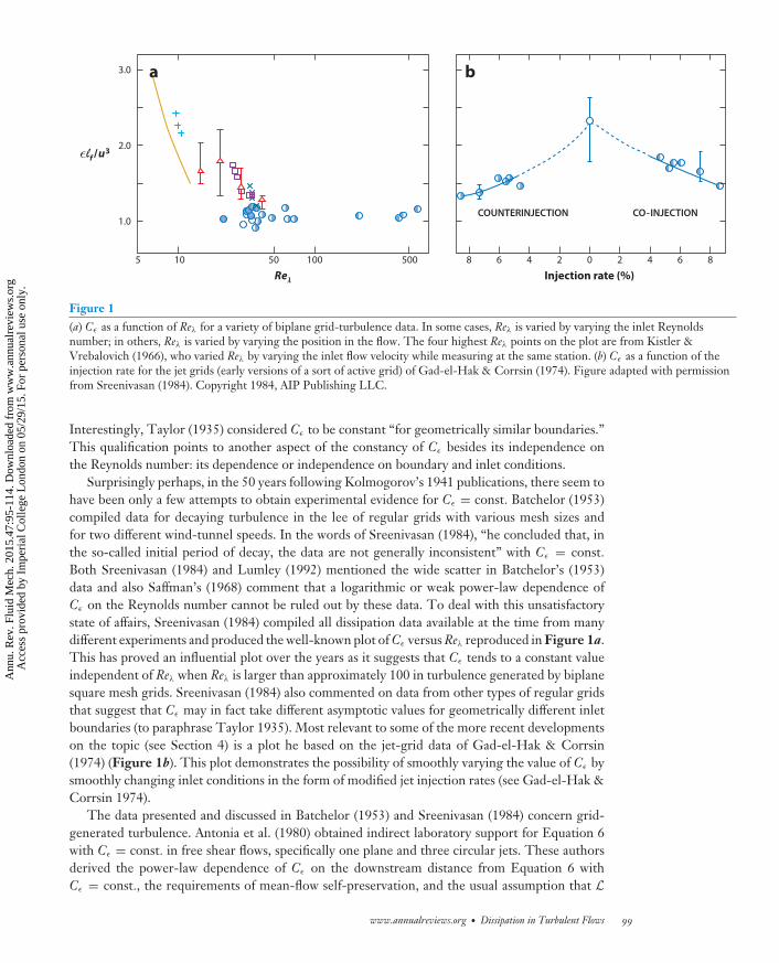
Figure 1(a) Cε as a function of Reλ for a variety of biplane grid-turbulence data. In some cases, Reλ is varied by varying the inlet Reynoldsnumber; in others, Reλ is varied by varying the position in the flow. The four highest Reλ points on the plot are from Kistler &Vrebalovich (1966), who varied Reλ by varying the inlet flow velocity while measuring at the same station. (b) Cε as a function of theinjection rate for the jet grids (early versions of a sort of active grid) of Gad-el-Hak & Corrsin (1974). Figure adapted with permissionfrom Sreenivasan (1984). Copyright 1984, AIP Publishing LLC.

Interestingly, Taylor (1935) considered Cε to be constant “for geometrically similar boundaries.”This qualification points to another aspect of the constancy of Cε besides its independence onthe Reynolds number: its dependence or independence on boundary and inlet conditions.

Surprisingly perhaps, in the 50 years following Kolmogorov’s 1941 publications, there seem tohave been only a few attempts to obtain experimental evidence for Cε = const. Batchelor (1953)compiled data for decaying turbulence in the lee of regular grids with various mesh sizes andfor two different wind-tunnel speeds. In the words of Sreenivasan (1984), “he concluded that, inthe so-called initial period of decay, the data are not generally inconsistent” with Cε = const.Both Sreenivasan (1984) and Lumley (1992) mentioned the wide scatter in Batchelor’s (1953)data and also Saffman’s (1968) comment that a logarithmic or weak power-law dependence ofCε on the Reynolds number cannot be ruled out by these data. To deal with this unsatisfactorystate of affairs, Sreenivasan (1984) compiled all dissipation data available at the time from manydifferent experiments and produced the well-known plot of Cε versus Reλ reproduced in Figure 1a.This has proved an influential plot over the years as it suggests that Cε tends to a constant valueindependent of Reλ when Reλ is larger than approximately 100 in turbulence generated by biplanesquare mesh grids. Sreenivasan (1984) also commented on data from other types of regular gridsthat suggest that Cε may in fact take different asymptotic values for geometrically different inletboundaries (to paraphrase Taylor 1935). Most relevant to some of the more recent developmentson the topic (see Section 4) is a plot he based on the jet-grid data of Gad-el-Hak & Corrsin(1974) (Figure 1b). This plot demonstrates the possibility of smoothly varying the value of Cε bysmoothly changing inlet conditions in the form of modified jet injection rates (see Gad-el-Hak &Corrsin 1974).

The data presented and discussed in Batchelor (1953) and Sreenivasan (1984) concern grid-generated turbulence. Antonia et al. (1980) obtained indirect laboratory support for Equation 6with Cε = const. in free shear flows, specifically one plane and three circular jets. These authorsderived the power-law dependence of Cε on the downstream distance from Equation 6 withCε = const., the requirements of mean-flow self-preservation, and the usual assumption that L


Ann

u. R

ev. F

luid

Mec

h. 2

015.

47:9

5-11

4. D

ownl

oade

d fr

om w

ww

.ann

ualr

evie

ws.

org

Acc

ess

prov

ided

by

Impe

rial

Col

lege

Lon

don

on 0

5/29

/15.

For

per

sona

l use

onl

y.


is well represented by the jet width. They then showed that their data confirmed the predicteddownstream variation of Cε .

4. EVIDENCE FOR ε ∼ U3/L IN THE PAST 25 YEARS

There have been several developments since Lumley’s (1992) review of the experimental evidenceconcerning Cε : (a) Sreenivasan’s (1995, 1998) updates and the advent of direct numerical simu-lations (DNS) capable of reaching Reynolds numbers large enough for meaningful tests of theconstancy of Cε in Equation 6, (b) a mathematically rigorous upper bound on dissipation that em-ulates Equation 6, (c) a new confined flow experiment originating from France, (d ) contributionsby Antonia and colleagues on the nonuniversality of the high–Reynolds number value of Cε , (e) arelation between Cε and a dimensionless number characterizing the number of large-scale eddiesper integral scale, and ( f ) a distinction between decaying and forced homogeneous turbulence asfar as Cε is concerned and a new dissipation law for nonequilibrium turbulence.

Sreenivasan (1995) examined data from homogeneous shear flows and cylinder wakes. As inBatchelor (1953) and Sreenivasan (1984), the surrogates used for U and L in Equation 6 werethe multiple of the root-mean-square streamwise turbulence fluctuating velocity

√3/2u′

1 and thelongitudinal integral length scale L11. For homogeneous shear flows, Sreenivasan (1995) concludedthat Cε tends to a value independent of Reλ as Reλ increases above 100 but that Cε is neverthelessweakly dependent on the shear. His turbulent wake data were obtained at a distance of 50 cylinderdiameters from the wake-generating cylinder. There, Cε proved to be independent of the inletReynolds number Re D = U ∞ D/ν, with U ∞ the fluid velocity upstream of the cylinder and D itsdiameter, for values of ReD larger than approximately 1,000.

In Sreenivasan’s (1998) update on Cε , he examined data from DNS of homogeneous turbulencein a periodic box. This time Cε was calculated from Equation 6 by taking U2 to be the totalkinetic energy of the turbulence and L to be the integral length scale corresponding to the three-dimensional spectrum. With the exception of just three Cε values that were from DNS of decayingturbulence, all other DNS of incompressible turbulence included a large-scale forcing in theNavier-Stokes equation to keep the turbulence at a statistically stationary state. The conclusionwas that Cε does indeed tend to a value independent of Reλ for Reλ > 100 but that this value maysignificantly differ for different large-scale forcings. Kaneda et al. (2003) carried out similar DNSof forced periodic turbulence at much higher Reynolds numbers and confirmed the Reynoldsnumber independence of Cε (calculated as in Sreenivasan 1998) up to Reλ ≈ 1,200.

Remaining in the realm of periodic forced Navier-Stokes turbulence, Doering & Foias (2002)rigorously proved from the incompressible Navier-Stokes equations that periodic and statisticallystationary body-forced three-dimensional turbulence is such that ε ≤ c 1νU/ l2 + c 2U3/ l , where c1

and c2 are dimensionless Reynolds number–independent coefficients, and l is the longest lengthscale in the applied forcing assumed square-integrable. In the high–Reynolds number limit whereν → 0, this inequality is remarkably comparable to Equation 6. Rollin et al. (2011) showed thatthe high–Reynolds number value of the normalized dissipation rate depends on the shape ofthe low-wave-number forcing and that this shape dependence is captured by the upper-boundanalysis. For a review of the three-dimensional Navier-Stokes problem and for references to otherdissipation-rate bounds, the reader is referred to Doering (2009).

The DNS data in Sreenivasan (1998) and Kaneda et al. (2003) and the rigorous upper bound ofDoering & Foias (2002) were obtained for statistically stationary forced incompressible Navier-Stokes turbulence in a periodic domain. A good and accessible account of the Richardson-Kolmogorov cascade and its related statistical laws in such a setting has been given by Frisch(1995), and it differs from the summary account given in Section 2 of the present review. Section 2

100 Vassilicos

Ann

u. R

ev. F

luid

Mec

h. 2

015.

47:9

5-11

4. D

ownl

oade

d fr

om w

ww

.ann

ualr

evie

ws.

org

Acc

ess

prov

ided

by

Impe

rial

Col

lege

Lon

don

on 0

5/29

/15.

For

per

sona

l use

onl

y.


is concerned with the Richardson-Kolmogorov cascade for Equation 1, whereas Frisch (1995),Sreenivasan (1998), Kaneda et al. (2003), and Doering & Foias (2002) dealt with

∂

∂tu + u · ∇ξ u = −∇ξ p + ν∇2

ξ u + f , (8)

where f is a forcing term acting only at large scales. All these authors consider the situation inwhich <f ·u> = ε, and Frisch (1995) derived Kolmogorov’s famous 4/5 law, which is effectively thesame as Equation 5 with the extra assumption of small-scale isotropy, by making the assumptionthat Cε does not depend on the Reynolds number (see also Tchoufag et al. 2012 and Laizet et al.2013 for related yet different approaches). Equation 6 with Cε = const. is therefore a cornerstoneassumption on which the Richardson-Kolmogorov cascade rests in the setting studied by Frisch(1995) and is not a consequence of the Richardson-Kolmogorov cascade as in Section 2. Anotherimportant difference is that all the terms in Equation 6 are independent of the spatial location inFrisch (1995), whereas U and L are not in the setting of Section 2.

An experimental development that has proven very influential over the past 25 years in variousareas of investigation involving turbulent flow is the so-called French washing machine (Douadyet al. 1991). This apparatus consists of a cylindrical tank with two coaxial counter-rotating stirrersat the top and bottom of the tank. Cadot et al. (1997) were motivated to use it to check the high–Reynolds number validity of Equation 6 with Cε = const. by the absence of tests for this scalingin experiments in which statistically stationary turbulence is maintained in a closed container.To enhance the dissipation in the bulk of the fluid with respect to the boundary layers, theyused rough (inertial) stirrers. Unlike previous measurements by Batchelor (1953) and Sreenivasan(1984, 1995), who used hot-wire anemometry to obtain local fluctuating velocities, Cadot et al.(1997) measured the global energy dissipation εG by measurements of the rate of mean temperaturevariations and also independently measured the total power P needed to drive the disks. They variedthe global Reynolds number �R2/ν, where � and R are the rotation frequency and radius of thedisks, by varying � and by using different fluids with different viscosities. In all cases, they checkedthat P and εG closely balanced, and they plotted what effectively amounted to CεG ≡ (εG R)/(�R)3,which they found to be constant over more than three decades of �R2/ν (from 3 × 103 to 7 ×106). This experiment is perhaps the closest to the forced turbulence in a periodic box studiedwith DNS and mathematical analysis of the incompressible Navier-Stokes equations discussedabove.

Antonia and collaborators addressed the issue, first briefly mentioned by Taylor (1935) andsubsequently encountered in the data examined by Sreenivasan (1984, 1995, 1998), that Cε dependson inlet/boundary/flow conditions. Antonia & Pearson (2000) made hot-wire measurements intwo different two-dimensional wakes, one of a circular cylinder and one of a flat plate. Theyconsidered only one measurement station in each one of these wakes and varied the Reynoldsnumber by varying the inlet flow velocity. Following Batchelor (1953) and Sreenivasan (1984,1995), they calculated Cε by replacing U with

√3/2u′

1 and L with L11 in Equation 6. At anequal Reynolds number, Reλ, they found different values of Cε in different wakes, even thoughtheir measuring stations were deemed to be far from the wake generator, 54 and 62 diametersdownstream of the cylinder and flat plate, respectively.

Burattini et al. (2005) extended the study to even more two-dimensional wakes, also looked atdata from regular and active grid turbulence and homogeneous shear flow, and reported a widevariability of Cε , between 0.5 and 2.5 for Reλ > 50. They assigned this variability to a dependenceon the flow configuration but not to a dependence on the Reynolds number. Boffetta & Romano(2002) took measurements at a streamwise distance of 40 jet diameters from a round jet exit andreported that Cε does not vary with Reλ over a wide range of Reλ values.


Ann

u. R

ev. F

luid

Mec

h. 2

015.

47:9

5-11

4. D

ownl

oade

d fr

om w

ww

.ann

ualr

evie

ws.

org

Acc

ess

prov

ided

by

Impe

rial

Col

lege

Lon

don

on 0

5/29

/15.

For

per

sona

l use

onl

y.


By making use of the Rice theorem, which was brought into the study of turbulence byLiepmann (1949) and Liepmann & Robinson (1952), Mazellier & Vassilicos (2008) establisheda relation between Cε and a dimensionless number C ′

s , which characterizes the large-scale flowtopology of the turbulence. C ′

s is effectively a number of large-scale eddies within an integral scaleand is dependent on inlet/flow conditions. It is therefore not universal. Turbulence fluctuationsbeing statistically self-similar, the small number of large scales is directly reflected in the largenumber of small scales. A way to quantify these numbers is to count zero crossings of both thesignal itself and filtered versions of it. The average distance l between zero crossings is thereforestrongly influenced by C ′

s [Mazellier & Vassilicos (2008) gave a precise definition of C ′s ], and by

virtue of the Rice theorem, this average distance l is proportional to the Taylor microscale λ, itselfdirectly related to ε. It then follows that Cε ∝ C ′3

s (see Mazellier & Vassilicos 2008 for detailedexplanations). The strong flow/inlet dependence of Cε already observed in previous investigationscan therefore be quantified as a dependence on C ′

s , which is naturally dependent on flow/inletconditions. This approach allowed Mazellier & Vassilicos (2008) to collapse 30 different Cε valuesfrom seven different turbulent flows. Note that Mouri et al. (2012) and Thiesset et al. (2014) alsofound a significant dependence of Cε on flow/inlet conditions, but they claimed that it was causedby the wrong choice of L to characterize the size of the large-scale energy-containing eddies.Mouri et al. (2012) collapsed 17 different Cε values from three different turbulent flows by usingthe integral length scale of u2

1 −<u21> instead of Batchelor’s (1953) L11 choice of L. Thiesset et al.

(2014) collapsed 15 different such values (all measured in turbulent wakes at the same normalizeddistance from five different obstacles but with various inlet Reynolds numbers) by using a cross-over length scale that is intermediate between energy injection and maximum interscale energytransfer. The links between these two approaches and with the one based on the Rice theoremhave not yet been investigated.

Goto & Vassilicos (2009) generalized the Rice theorem to stagnation points of a statisticallyhomogeneous and isotropic incompressible fluctuating velocity field and showed that λ = Bls ,where ls is the average distance between stagnation points, and B is a dimensionless number with avery weak dependence on the Reynolds number caused by small-scale intermittency. In terms of anumber Cs of large-scale stagnation points per integral scale [Goto & Vassilicos (2009) defined Cs

in a precise way that generalizes C ′s ], they showed that Cε ∼ Cs /B3. They then addressed the issue

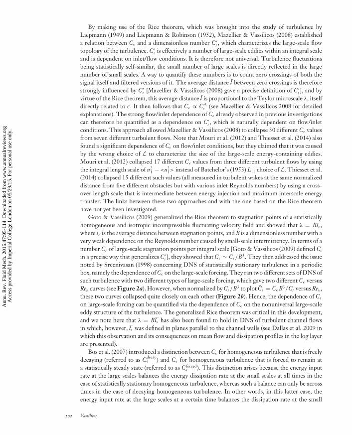
noted by Sreenivasan (1998) concerning DNS of statistically stationary turbulence in a periodicbox, namely the dependence of Cε on the large-scale forcing. They ran two different sets of DNS ofsuch turbulence with two different types of large-scale forcing, which gave two different Cε versusReλ curves (see Figure 2a). However, when normalized by Cs /B3 to plot Cε = Cε B3/Cs versus Reλ,these two curves collapsed quite closely on each other (Figure 2b). Hence, the dependence of Cε

on large-scale forcing can be quantified via the dependence of Cε on the nonuniversal large-scaleeddy structure of the turbulence. The generalized Rice theorem was critical in this development,and we note here that λ = Bls has also been found to hold in DNS of turbulent channel flowsin which, however, ls was defined in planes parallel to the channel walls (see Dallas et al. 2009 inwhich this observation and its consequences on mean flow and dissipation profiles in the log layerare presented).

Bos et al. (2007) introduced a distinction between Cε for homogeneous turbulence that is freelydecaying (referred to as Cdecay

ε ) and Cε for homogeneous turbulence that is forced to remain ata statistically steady state (referred to as C forced

ε ). This distinction arises because the energy inputrate at the large scales balances the energy dissipation rate at the small scales at all times in thecase of statistically stationary homogeneous turbulence, whereas such a balance can only be acrosstimes in the case of decaying homogeneous turbulence. In other words, in this latter case, theenergy input rate at the large scales at a certain time balances the dissipation rate at the small

102 Vassilicos

Ann

u. R

ev. F

luid

Mec

h. 2

015.

47:9

5-11

4. D

ownl

oade

d fr

om w

ww

.ann

ualr

evie

ws.

org

Acc

ess

prov

ided

by

Impe

rial

Col

lege

Lon

don

on 0

5/29

/15.

For

per

sona

l use

onl

y.


ba

Reλ Reλ50 100 150 200 50 100 150 200

0.48

0.52

0.56

0.60

C C~

0

0.005

0.010

0.015

0.020

Figure 2(a) Cε as a function of Reλ from direct numerical simulations of forced periodic statistically stationary turbulence. Closed and opensymbols correspond to different large-scale forcing procedures. (b) Cε = Cε B3/Cs as a function of Reλ for the same data. Figureadapted with permission from Goto & Vassilicos (2009). Copyright 2009, AIP Publishing LLC.

scales at a later time, with the difference between these two times being the time needed forthe energy to cascade from large to small scales. These considerations expressed in equationslead to Cdecay

ε �= C forcedε . Bos et al. (2007) tested their ideas against DNS, large-eddy simulations,

and the EDQNM (eddy-damped quasi-normal Markovian) spectral closure and found differencesbetween Cdecay

ε and C forcedε , which add to the body of evidence suggesting that Cε in Equation 6 is

not universal in the sense that it depends on inlet/boundary conditions and the type of flow.The standard attempt at generating decaying homogeneous turbulence in the laboratory in-

volves a grid placed at the inlet of a wind tunnel’s test section, the so-called grid turbulence. In suchexperiments, the role of time is played by the streamwise distance x from the grid, and the consid-erations of Bos et al. (2007) imply a value of Cdecay

ε different from C forcedε but also invariant with x.

In fact, the fundamental reason for this invariance with x is the Reynolds number independenceof Cε and that the local Reynolds number decays with increasing x. Several recent investigationsdiscussed below have unveiled a type of decaying grid turbulence in which Cε is not constant butin fact increases with x, even though the local Reynolds number does indeed decay with x.

5. THE NONEQUILIBRIUM DISSIPATION LAW

Grid-turbulence experiments in wind tunnels and water flumes using both hot-wire anemometryand particle image velocimetry have shown that a significant turbulence decay region exists inwhich E11(k1) ∼ k−5/3

1 over more than a decade of wave numbers, yet Cε ∼ RemI /Ren

L ( �= const.),with m ≈ 1 ≈ n, Re I = (U ∞Lb )/ν, and Re L = (u′

1 L11)/ν (Seoud & Vassilicos 2007, Mazellier &Vassilicos 2010, Valente & Vassilicos 2011, Gomes-Fernandes et al. 2012, Valente & Vassilicos2012, Discetti et al. 2013, Nagata et al. 2013, Hearst & Lavoie 2014, Isaza et al. 2014, Valente &Vassilicos 2014). ReI is a global or inlet Reynolds number based on the inlet flow speed U ∞ anda length scale Lb defined by the grid and does not depend on the local position in the flow. ReL isa local Reynolds number that can, and does, differ from place to place in the flow.

Seoud & Vassilicos (2007) obtained the first evidence of a very different dissipation scalingin the decaying turbulence generated by some of the fractal square grids introduced by Hurst &


Ann

u. R

ev. F

luid

Mec

h. 2

015.

47:9

5-11

4. D

ownl

oade

d fr

om w

ww

.ann

ualr

evie

ws.

org

Acc

ess

prov

ided

by

Impe

rial

Col

lege

Lon

don

on 0

5/29

/15.

For

per

sona

l use

onl

y.


Vassilicos (2007). They recorded how u′21 , L11, and ε vary as functions of the streamwise distance

from the grid. They also found that, along the centerline, Cε = εL11/u′31 increases as ReL decreases

in such a way that Cε ∼ Re−1L , even though the energy spectrum of the turbulence has a power-law

range over more than a decade with an exponent very close, if not equal, to −5/3. In particular,they reported that L11/λ remains constant as ReL and Reλ decay, which follows from Equation 7and Cε ∼ Re−1

L . As mentioned in Section 2, the Richardson-Kolmogorov cascade is such thatthe range of length scales required for the turbulent energy to dissipate increases with increasingReynolds number. This is not the case in the region of the flow that Seoud & Vassilicos (2007)investigated.

Mazellier & Vassilicos (2010) followed this work by noting that the actual constant valueof L11/λ is in fact an increasing function of the inlet Reynolds number and that the relationCε ∼ Re−1

L is increasingly clear with increasing ReI (see Figure 3). They also introduced the wakeinteraction length scale x∗ [revised and improved by Gomes-Fernandes et al. (2012)], which canbe calculated from the geometry of the grid to predict the furthest point downstream (the oneon the centerline with streamwise coordinate xpeak) beyond which the turbulence decays. As seenin Figure 3, the local Reynolds number increases from x = 0, where the grid is placed untilapproximately x = 0.4x∗, and then decays in the region x > 0.4x∗. The new dissipation behaviorhas been documented in a sizeable part of the decay region, x > 0.4x∗. To give an idea of the size,Gomes-Fernandes et al. (2012) confirmed that L11/λ remains constant while Reλ decays betweenx = xpeak and x = 3xpeak in a water channel of 0.6 m × 0.6 m cross-sectional area, where thefractal square grid used was such that xpeak = 1.4 m. The new dissipation behavior was thereforepresent between 1.4 m and 4.2 m from the grid in this channel. These authors were not able

ba

ReλLu /λ

x/x* x/x*

0

2

4

6

8

10

12

U∞ = 5.2 m/sU∞ = 10 m/sU∞ = 15 m/s

0 0.2 0.4 0.6 0.8 1.0 1.20

50

100

150

200

250

300

350

400

450

0 0.2 0.4 0.6 0.8 1.0 1.2

Figure 3(a) Ratio of the longitudinal integral length scale L11 to the Taylor microscale λ as a function of the streamwise distance x from aturbulence-generating fractal square grid along the centerline. The distance x is normalized by the wake interaction length scale x∗introduced by Mazellier & Vassilicos (2010) and Gomes-Fernandes et al. (2012) as a predictor of the streamwise distance from the gridwhere the turbulence intensity peaks (around x/x∗ ≈ 0.4 in this case). Note the constancy of L11/λ in the decay region x/x∗ > 0.4 andthe increasing constant value of L11/λ with increasing inlet flow speed U ∞. (b) Reλ as a function of x/x∗ for the same grid and the samethree different values of U ∞ = 5.2 m/s, 10 m/s, and 15 m/s. Figure adapted with permission from Mazellier & Vassilicos (2010).Copyright 2010, AIP Publishing LLC.

104 Vassilicos

Ann

u. R

ev. F

luid

Mec

h. 2

015.

47:9

5-11

4. D

ownl

oade

d fr

om w

ww

.ann

ualr

evie

ws.

org

Acc

ess

prov

ided

by

Impe

rial

Col

lege

Lon

don

on 0

5/29

/15.

For

per

sona

l use

onl

y.


to make measurements further downstream to determine the length of this region with unusualdissipation scaling.

Various profiles of one-point statistics have been extensively documented in the lee of fractalsquare grids (specifically high–thickness ratio, low-blockage, space-filling fractal square grids; seereferences below for these qualifications), and they have been reported by Hurst & Vassilicos(2007), Seoud & Vassilicos (2007), Mazellier & Vassilicos (2010), Valente & Vassilicos (2011),Nagata et al. (2013), and Discetti et al. (2013). The salient conclusions of these homogeneityinvestigations are that the turbulence is highly inhomogeneous and non-Gaussian in the pro-duction region close to the grid (i.e., x < xpeak) and then only weakly inhomogeneous (if notapproximately homogeneous) and close to Gaussian in the decay region (x > xpeak) around thecenterline, except for third-order moments, meaning that there is nonnegligible transverse energyand pressure transport. The isotropy/anisotropy characteristics in the decay region are broadlysimilar to those of regular grids. The streamwise extent over which the new dissipation scaling isreported around the centerline extends over a number of eddy turnover times, and the timescalesof the energy-containing eddies are significantly smaller than the inverse mean flow gradients.

Valente & Vassilicos (2012) applied the wake interaction length scale to the design of tworegular grids with unusually low blockage and a small number of meshes but with a value ofxpeak larger than that of usual regular grids and comparable to that of previously used fractalsquare grids in the same wind-tunnel test section. This allowed a fair comparison between regulargrid and fractal square grid turbulence in the same range of x/xpeak values for which the newdissipation scaling has been observed for fractal square grids. They concluded that their unusualregular grids display the same dissipation scaling in the decay region as the fractal square grids(i.e., Cε = εL11/u′3

1 increases while ReL decreases so that Cε ∼ Re−1L and so that L11/λ remains

constant while ReL decays). Again, as with fractal square grids, this behavior is accompanied bya very well-defined −5/3 turbulence energy spectrum, even though the Richardson-Kolmogorovcascade as we know it does not imply such a Reynolds number dependence on Cε , nor does itimply a constant ratio of scales as the local Reynolds number decays.

Valente & Vassilicos (2012) also used a fractal square grid and a usual regular grid for twopurposes: (a) to confirm and quantify Mazellier & Vassilicos’s (2010) observation that the constantvalue of L11/λ increases with global/inlet Reynolds number ReI [Mazellier & Vassilicos (2010) hadactually noted that this length-scale ratio is proportional to the square root of an inlet Reynoldsnumber in all canonical free shear flows] and (b) to take advantage of the usual regular grid’s smallvalue of xpeak to explore how far downstream the new dissipation scalings hold in multiples of xpeak.Their measurements showed that Cε ∼ Rem

I /RenL, with m ≈ 1 ≈ n and Lb in Re I = (U ∞Lb )/ν

being the largest mesh size on the grid (which is the actual mesh size in the case of regular grids). Inthe case of their usual regular grid, this new dissipation law was found to hold in xpeak < x < 5xpeak,with Cε adopting a constant value at x > 5xpeak (see Figure 4a). Subsequently, these findings wereconfirmed by Isaza et al. (2014) with a usual regular grid of their own and by Hearst & Lavoie(2014) with a grid made of many repetitions of a fractal square grid so as to bring the value ofxpeak down and probe a very wide range of x/xpeak in fractal-generated decaying turbulence (seeFigure 4b). Valente & Vassilicos (2014) surveyed various turbulent profiles in the decay region ofvarious fractal and regular grids and showed that the new dissipation scaling is present irrespectiveof significant inhomogeneity and anisotropy differences between their grids. They also verifiedthat this new dissipation scaling is not an artifact of anisotropy by trying different transverse andlongitudinal surrogates for U and L.

Section 2 ends with a reminder that the equilibrium dissipation relation given in Equation 6with Cε = const. effectively determines the streamwise development of mean profiles of self-preserving turbulent free shear flows (Townsend 1976, George 1989). In such flows, U scales


Ann

u. R

ev. F

luid

Mec

h. 2

015.

47:9

5-11

4. D

ownl

oade

d fr

om w

ww

.ann

ualr

evie

ws.

org

Acc

ess

prov

ided

by

Impe

rial

Col

lege

Lon

don

on 0

5/29

/15.

For

per

sona

l use

onl

y.


25 30 35 40 45 50 55 60 65 70 75 80

C

x/L0

b

C

ReM/ReL

a

0.4

0.5

0.6

0.7

0.8

0.9

1.0

1.1

5 10 15 20 25 30 35 40 45 500.4

0.5

0.6

0.7

0.8

0.9

1.0

1.1

x/x*

Figure 4(a) Cε versus Re I /Re L for a regular grid in which Re I = Re M = U ∞ M /ν as Lb is taken to be the mesh size M. Different symbolscorrespond to different values of ReI . The streamwise distance from the grid is indicated in the plot and increases with increasingRe I /Re L . The sudden change from Cε ∼ Re I /Re L to Cε ≈ const. occurs at x ≈ 5xpeak. Panel a adapted with permission from Valente& Vassilicos (2012). (b) Cε versus x/L0 for a square-fractal-element grid, where L0 is the size of each square fractal element on the grid.The open symbols are for two different values of the inlet flow speed U ∞, and the closed symbols are data from Valente & Vassilicos(2011) for a regular grid and a fractal square grid at different values of U ∞. Panel b adapted from Hearst & Lavoie (2014) withpermission from Cambridge University Press.

106 Vassilicos

Ann

u. R

ev. F

luid

Mec

h. 2

015.

47:9

5-11

4. D

ownl

oade

d fr

om w

ww

.ann

ualr

evie

ws.

org

Acc

ess

prov

ided

by

Impe

rial

Col

lege

Lon

don

on 0

5/29

/15.

For

per

sona

l use

onl

y.


x /θx /θ

a b

0 50 100 150 2000 50 100 150 2000

5

10

15

20

25

30

35

40

45

(δ/θ)2

0

5

10

15

20

25

30

35

40

45

(u0/U∞)–1

Figure 5Plots corresponding to the turbulent axisymmetric and self-preserving wake of a plate with an irregular periphery: (a) (u0/U ∞)−1

versus x/θ and (b) (δ/θ )2 versus x/θ , where u0 is the centerline mean velocity deficit, U ∞ is the constant upstream flow velocity, δ is thewake width, θ is the constant momentum thickness, and x is the streamwise distance from the wake-generating plate. Note that thelinear dependencies on x (over the x range considered) are in agreement with u0/U ∞ ∼ ((x − x0)/θ )−1 and δ/θ ∼ ((x − x0)/θ )1/2,which follow from the nonequilibrium dissipation scalings. Figure adapted with permission from Nedic et al. (2013).

with the centerline mean velocity deficit u0, and the integral scale is taken to be proportionalto the wake width δ. The Richardson-Kolmogorov cascade scaling Cε = const. then impliesu0/U ∞ ∼ ((x − x0)/θ )−2/3 and δ/θ ∼ ((x − x0)/θ )1/3 for turbulent axisymmetric wakes, where U ∞is the constant upstream flow velocity, and θ is the constant momentum thickness (see Townsend1976, George 1989). Nedic et al. (2013) used the new dissipation scaling Cε ∼ Rem

I /RenL with m =

n = 1 to derive its corresponding turbulent axisymmetric wake laws and found the very differentscalings u0/U ∞ ∼ ((x − x0)/θ )−1 and δ/θ ∼ ((x − x0)/θ )1/2. They then carried out wind-tunneltests of axisymmetric wakes generated by plates with irregular peripheries placed normal to anincoming free stream and found that these new wake laws are present and very well defined ina downstream streamwise range between approximately 5

√A and at least 50

√A, where A is the

area of the plate (see Figure 5). The turbulence decays in this streamwise wake region, and onemay expect a transition further downstream to the usual wake laws that stem from the equilibriumdissipation scaling Cε = const.

Some of the authors of the aforementioned papers referred to the new dissipation scalingCε ∼ Rem

I /RenL, with m ≈ 1 ≈ n, as a nonequilibrium turbulence dissipation law because it

violates the Richardson-Kolmogorov cascade’s suggestion that Cε = const. and also appears tohold in various turbulent flows. It may be surprising to find the same dissipation law in differentnonequilibrium decay regions of different turbulent flows. Actually, the exact values of n and m,even if close to 1, remain to be investigated, including the possibility that there may be somevariations from flow to flow.

Concerning the nonequilibrium qualification of this new dissipation scaling, there are re-ally three assumptions leading to Equation 6 with Cε = const. in nonstationary turbulence (seeSection 2). The major ones are local homogeneity and Kolmogorov’s equilibrium hypothesis,but the third one (see Section 2) is the extrapolation of the equilibrium cascade relation given in


Ann

u. R

ev. F

luid

Mec

h. 2

015.

47:9

5-11

4. D

ownl

oade

d fr

om w

ww

.ann

ualr

evie

ws.

org

Acc

ess

prov

ided

by

Impe

rial

Col

lege

Lon

don

on 0

5/29

/15.

For

per

sona

l use

onl

y.


Equation 5 to r ∼ L. [Kolmogorov (1941b) actually made such an assumption too.] One cannotrule out the possibility that, in the region where the nonequilibrium dissipation law holds, theassumption at fault is in fact this third one. If that is the case, then this would also be an equilibriumfailure, although not necessarily over the entire range of scales, only at the high end of it. Hence,the nonequilibrium qualification remains meaningful. Furthermore, if the equilibrium hypothesisand Equation 5 remain valid but only at much smaller values of r, then the nonequilibrium dissi-pation law would imply that the spherically averaged interscale energy flux strongly depends onthe inlet Reynolds number, which violates the universality aspect of the Richardson-Kolmogorovcascade in a rather uniquely dramatic and explicit way. Either way, the nonequilibrium scalingsignifies that the interscale energy transfers do not add up to a classical Richardson-Kolmogorovcascade in the region where this law is observed. If there is a cascade of sorts, and there mostprobably is, it is of a different type.

6. CONCLUSION AND DISCUSSION

There is a difference between forced statistically stationary turbulence in a periodic or closed box,on the one hand, and time/space-varying turbulence, in particular decaying turbulence, on theother. The DNS results reported by Sreenivasan (1998) and Kaneda et al. (2003), the inequalityderived from the Navier-Stokes equation by Doering & Foias (2002), and the closed-containerexperiments of Cadot et al. (1997) lend strong support to Equation 6 with Cε = const. in thecontext of forced statistically stationary turbulence in a box. In fact, in all these cases, U and L areindependent of both space and time.

The situation appears to differ when the turbulence is decaying, both in a self-preservingaxisymmetric turbulent wake and in decaying grid-generated turbulence apparently irrespectiveof the grid. As soon as the turbulence starts decaying along the streamwise direction in these flows,the normalized dissipation coefficient Cε is found to be growing while the local Reynolds numbersReL and Reλ are decreasing. This behavior is not the one suggested by the Richardson-Kolmogorovcascade, even though the energy spectra exhibit their best −5/3 wave-number scalings over thewidest wave-number range in this nonequilibrium decay region where Cε ∼ Rem

I /RenL, with

m ≈ 1 ≈ n. In the few cases in which it has been possible to go far enough downstream in terms ofthe relevant length scale (xpeak), a sudden transition is observed to Cε = const. Still, this constancyis in terms of the streamwise distance x and local Reynolds number, not necessarily in terms of theinlet conditions. As Taylor (1935) seems to have expected and as a number of authors have shown,starting with Sreenivasan and Antonia and his colleagues, Cε can take different Reynolds number–independent values for different inlet/boundary conditions and different types of flow. Recently,Thormann & Meneveau (2014) substantially added to this bank of nonuniversality evidence withtheir extensive study of turbulence generated by various types of active fractal grids, which showedthat Cε differs for different inlet conditions. In doing so, they introduced new types of turbulentflows that will help future research developments.

It is essential for the observation of the nonequilibrium dissipation scaling to conduct experi-ments in which values of Cε are recorded by varying both the global/inlet Reynolds number ReI

and the streamwise measurement location so as to vary the local Reynolds numbers ReL and Reλ

without varying ReI . Kistler & Vrebalovich (1966) obtained the four highest Reλ data points inFigure 1a by measuring at one single point in the flow and varying the inlet Reynolds numberReI only. Such measurements would return a value of Cε that is more or less independent of theReynolds number, irrespective of the position of the measuring station with respect to xpeak, eitherbecause Cε is indeed constant or because Cε ∼ Rem

I /RenL, with m ≈ 1 ≈ n, and ReL increases

linearly with ReI . Without these four high–Reynolds number data points, Figure 1a is left with

108 Vassilicos

Ann

u. R

ev. F

luid

Mec

h. 2

015.

47:9

5-11

4. D

ownl

oade

d fr

om w

ww

.ann

ualr

evie

ws.

org

Acc

ess

prov

ided

by

Impe

rial

Col

lege

Lon

don

on 0

5/29

/15.

For

per

sona

l use

onl

y.


only one data point at an Reλ larger than 100 and is therefore much less, if at all, conclusive as to theconstancy of Cε . The importance of varying ReI and ReL independently for conclusive statementson Cε has only surfaced in the past eight or so years.

One might be tempted to dismiss the new nonequilibrium dissipation scaling as a transientin space, even though it is, of course, not a transient in time in the flows in which it has beenrecorded. The nonequilibrium decay region is a well-defined, permanently present region inthe lee of various turbulent flows that may not extend all the way downstream to the ultimateregion where the flow may cease to be turbulent in a spectral sense (at least it is not known toextend so far in any flow to date). More to the point, this well-defined, permanently presentregion has similar, if not the same, dissipation scaling laws in a variety of turbulent flows andcan therefore not be dismissed as unworthy of study. In some cases, the transition from thisnonequilibrium decay region to a further downstream decay region where Cε is independent ofthe local Reynolds number has been detected. The Kolmogorov −5/3 wave-number scaling ofthe spectrum in the decay region is at its clearest over the widest range of wave numbers in thenonequilibrium region where the local Reynolds number is higher than it is further downstream,yet the Richardson-Kolmogorov cascade does not seem to be the cascade or interscale energytransfer mechanism at work. In fact, Laizet et al. (2013) and Gomes-Fernandes et al. (2014a,b)have traced the existence of well-defined Kolmogorov −5/3 spectra to the highly inhomogeneousand non-Gaussian production region very close to the turbulence-generating grid (upstream ofthe entire decay region) where, according to Gomes-Fernandes et al.’s (2014b) particle imagevelocimetry analysis of the nonhomogeneous nonisotropic Karman-Howarth-Monin equation(Equation 2), the cascade is inverse along an axis at a small angle to the streamwise direction andforward in the transverse direction. This combined forward-inverse cascade is definitely not acharacteristic of the Richardson-Kolmogorov cascade, yet it appears in conjunction with a −5/3streamwise energy spectrum. Power-law energy spectra with exponents close to −5/3 have alsobeen reported in a cylinder wake within 1 cylinder diameter from the cylinder (Braza et al. 2006).Of course, it will be important in the future to carefully check the relation between the frequencyand wave-number domains in such close-proximity flow regions.

Along with the production region, the nonequilibrium region is not only important funda-mentally, it can also be expected to matter in many industrial, engineering, and environmentalcontexts, far more than the very far region beyond it. Nedic et al. (2013) recorded nonequilibriumwake scalings up to a distance of 50

√A, where A is the area of the wake-generating plate (see

Section 5). This is a very long way downstream for many practical purposes, and new approacheswill need to be developed to model the turbulence there. We are reminded of the quotation fromLumley (1992) at the start of this review: “What part of modeling is in serious need of work?Foremost, I would say, is the mechanism that sets the level of dissipation in a turbulent flow,particularly in changing circumstances.”

The changing circumstances can be gradual, perhaps caused by no more than gradual turbu-lence decay, or sudden, as at the point downstream at which the turbulence suddenly transits fromCε ∼ Rem

I /RenL, with m ≈ 1 ≈ n, to Cε = const. (see Figure 4). There are several length scales

that are beginning to surface in importance, such as xpeak and the wake interaction length scalethat aims to predict xpeak in grid-generated turbulence. The point at which the aforementionedsudden change occurs is a multiple of xpeak, perhaps 5xpeak as in one of the regular grid experimentsof Valente & Vassilicos (2012). An important question involves understanding the physical natureof this sudden change and the scalings of the point downstream where it happens. Related aresimilar questions for axisymmetric self-preserving turbulent wakes: What is the length scale atwhich the nonequilibrium scalings of the wake transit to the usual scalings, and what causes thissudden high to less high Reynolds number transition? The practical relevance and applications of


Ann

u. R

ev. F

luid

Mec

h. 2

015.

47:9

5-11

4. D

ownl

oade

d fr

om w

ww

.ann

ualr

evie

ws.

org

Acc

ess

prov

ided

by

Impe

rial

Col

lege

Lon

don

on 0

5/29

/15.

For

per

sona

l use

onl

y.


nonequilibrium turbulence depend quite critically on these length scales and our ability to predictthem from the geometry of inlet/boundary conditions. Investigations similar to that of Nedic et al.(2013) are now waiting to be made for other self-preserving turbulent free shear flows, such asjets, mixing layers, and other types of wakes, and similar questions may arise there too.

Recently, George (2014) advanced an argument suggesting that the Kolmogorov energy spec-trum scaling E(k) ∼ ε2/3k−5/3 is inconsistent with the Kolmogorov local equilibrium assump-tion for decaying homogeneous turbulence (the critical assumption that allows one to go fromEquation 4 to Equation 5 and obtain the Richardson-Kolmogorov cascade in nonstationary tur-bulence). His claim may be consistent with the unusual dissipation scalings in the nonequilibriumdecay region downstream of regular and fractal grids where the turbulence energy spectrum hasa well-defined −5/3 range. Further downstream where Cε = const., George’s (2014) claim (ifcorrect) would imply either an absence of a Kolmogorov spectral range or, if such a range doesexist [including both the ε2/3 and k−5/3 scalings of E(k)], a situation in which Cε = const. is not theresult of a high–Reynolds number Richardson-Kolmogorov cascade. Such far-downstream mea-surements are difficult because they require high local Reynolds numbers in a far region wherethe local Reynolds number has decayed. More work in this direction is required for the future,which may or may not produce evidence of a clear Cε = const. with respect to variations in bothReI and x in the far field combined with a clear well-defined Kolmogorov scaling range in theenergy spectrum. The active fractal grids of Thormann & Meneveau (2014) may prove usefulhere, particularly if the integral length scales returned by some of them are well defined.

Concerning the nonequilibrium decay region, self-preserving, single-scale spectral theoriesbased on the spectral equivalent of the Karman-Howarth-Monin equation (the so-called Linequation), such as those of George (1992) and George & Wang (2009), violate Kolmogorov’sequilibrium assumption and lead to Cε ∼ 1/Re L but not to Cε ∼ Re I /Re L, even though theyare not necessarily inconsistent with the latter. Mazellier & Vassilicos (2010) compared fractal-generated turbulence data from the nonequilibrium decay region with such theories (see alsoValente & Vassilicos 2011) and found good agreement but also found that the very small scalescan nevertheless be collapsed with the Kolmogorov microscale η, a feature that poses a challenge tothese theories. Following these developments, there is now an obvious and pressing need to directlyaddress the nature of the turbulence cascade and its scalings in nonequilibrium and in Cε = const.regions by studying interscale energy fluxes and balances in the nonhomogeneous, nonisotropicKarman-Howarth-Monin equation (Equation 2) or its spectral equivalent, if it can be meaningfullydefined. Bai et al. (2013) and P. Valente & J.C. Vassilicos (submitted manuscript) have startedaddressing this need. Bai et al. (2013) found that the measured energy flux is strongly dependenton the scale at the turbulent near-wake flow downstream of a fractal tree-like object; P. Valente& J.C. Vassilicos (submitted manuscript) found an important contribution of the unsteady termin Equation 2 albeit at relatively low Reynolds numbers in the nonequilibrium and Cε = const.regions of regular grids. Their experiment also confirms McComb et al.’s (2010) DNS result thatthe peak inertial flux scales as U3/L at relatively low Reynolds numbers.

FUTURE ISSUES

1. Other turbulent flows need to be explored for nonequilibrium non-Richardson-Kolmogorov cascades, such as DNS of periodic decaying or more generally statisticallyunsteady turbulence at high Reynolds numbers following McComb et al. (2010), whoseDNS was of low–Reynolds number periodic and decaying turbulence; DNS of periodicand decaying superfluid turbulence consisting of a normal viscous fluid interacting with

110 Vassilicos

Ann

u. R

ev. F

luid

Mec

h. 2

015.

47:9

5-11

4. D

ownl

oade

d fr

om w

ww

.ann

ualr

evie

ws.

org

Acc

ess

prov

ided

by

Impe

rial

Col

lege

Lon

don

on 0

5/29

/15.

For

per

sona

l use

onl

y.


a quantum inviscid vortex tangle via a mutual friction force (see Barenghi et al. 2014);and other boundary-free turbulent shear flows, such as various jets and mixing layersand other types of wakes, particularly those in which the local Reynolds number varieswith the downstream distance. Finally, what happens in wall turbulence? Could similarnonequilibrium dissipation regions be present there too?

2. What causes the sudden transition from Cε ∼ RemI /Ren

L, with m ≈ 1 ≈ n, to Cε = const.(see Figure 4), and what is the downstream distance where this happens? How can thisdownstream distance be estimated in terms of the geometry of the turbulence generatorand inlet Reynolds number? Is this distance related to the one at which one might expecta transition from the nonequilibrium wake laws of Figure 5 to the classical wake laws?What about other boundary-free shear flows? How close to the grid is the demarcationbetween production and decay regions in turbulence generated by jet grids (Gad-el-Hak & Corrsin 1974), active grids (Makita 1991), and active fractal grids (Thormann &Meneveau 2014), and is there also a nonequilibrium decay region in such turbulent flows?How can one use the spatiotemporal properties of such grids to estimate downstreamlength scales demarcating different regions?

3. What is “the mechanism that sets the level of dissipation in a turbulent flow, particularlyin changing circumstances”? This is a question that remains unanswered since Lumley(1992) asked it a quarter of a century ago, except that we now have a dissipation scalingfor nonequilibrium turbulence. How can we explain Cε ∼ Rem

I /RenL, with m ≈ 1 ≈ n,

and what are the properties of the interscale transfers and turbulence cascade that comewith it?

DISCLOSURE STATEMENT

The author is not aware of any biases that might be perceived as affecting the objectivity of thisreview.

ACKNOWLEDGMENTS

I am grateful to Professor Charles Doering and Dr. Oliver Buxton for the helpful commentsthey made on an early version of this article. I would also like to acknowledge the importantcontributions of Drs. Susumu Goto, Sylvain Laizet, and Nicolas Mazellier and of my PhD studentsDrs. Vassilis Dallas, Rafael Gomes-Fernandes, Daryl Hurst, Jovan Nedic, Richard Seoud, andPedro Valente in the research that we carried out together over the past 12 years or so.

LITERATURE CITED

Antonia RA, Pearson BR. 2000. Effect of initial conditions on the mean energy dissipation rate and the scalingexponent. Phys. Rev. E 62:8086–90

Antonia RA, Satyaprakash BR, Hussain AKMF. 1980. Measurements of dissipation rate and some othercharacteristics of turbulent plane and circular jets. Phys. Fluids 23:695–700

Bai K, Meneveau C, Katz J. 2013. Experimental study of spectral energy fluxes in turbulence generated by afractal, tree-like object. Phys. Fluids 25:110810

Barenghi CF, L’vov VS, Roche PE. 2014. Experimental, numerical, and analytical velocity spectra in turbulentquantum fluid. Proc. Natl. Acad. Sci. USA 111:4683–90

Batchelor GK. 1953. The Theory of Homogeneous Turbulence. Cambridge, UK: Cambridge Univ. Press


Ann

u. R

ev. F

luid

Mec

h. 2

015.

47:9

5-11

4. D

ownl

oade

d fr

om w

ww

.ann

ualr

evie

ws.

org

Acc

ess

prov

ided

by

Impe

rial

Col

lege

Lon

don

on 0

5/29

/15.

For

per

sona

l use

onl

y.


Boffetta G, Romano GP. 2002. Structure functions and energy dissipation dependence on Reynolds number.Phys. Fluids 14:3453–58

Bos WJT, Shao L, Bertoglio JP. 2007. Spectral imbalance and the normalized dissipation rate of turbulence.Phys. Fluids 19:045101

Braza M, Perrin R, Hoarau Y. 2006. Turbulence properties in the cylinder wake at high Reynolds numbers.J. Fluids Struct. 22:757–71

Burattini P, Lavoie P, Antonia RA. 2005. On the normalized turbulent energy dissipation rate. Phys. Fluids17:098103

Cadot O, Couder Y, Daerr A, Douady S, Tsinober A. 1997. Energy injection in closed turbulent flows: stirringthrough boundary layers versus inertial stirring. Phys. Rev. E 56:427–33

Dallas V, Vassilicos JC, Hewitt GF. 2009. Stagnation point von Karman coefficient. Phys. Rev. E 80:046306Danaila L, Krawczynski JF, Thiesset F, Renou B. 2012. Yaglom-like equation in axisymmetric anisotropic

turbulence. Physica D 241:216–23Discetti S, Ziskin IB, Astarita T, Adrian RJ, Prestridge KP. 2013. PIV measurements of anisotropy and

inhomogeneity in decaying fractal generated turbulence. Fluid Dyn. Res. 45:061401Doering CR. 2009. The 3D Navier-Stokes problem. Annu. Rev. Fluid Mech. 41:109–28Doering CR, Foias C. 2002. Energy dissipation in body-forced turbulence. J. Fluid Mech. 467:289–306Douady S, Couder Y, Brachet ME. 1991. Direct observation of the intermittency of intense vorticity filaments

in turbulence. Phys. Rev. Lett. 67:983–86Duchon J, Robert R. 2000. Inertial energy dissipation for weak solutions of incompressible Euler and Navier-

Stokes equations. Nonlinearity 13:249–55Eyink GL. 2003. Local 4/5-law and energy dissipation anomaly in turbulence. Nonlinearity 17:137–45Frisch U. 1995. Turbulence: The Legacy of A.N. Kolmogorov. Cambridge, UK: Cambridge Univ. PressGad-el-Hak M, Corrsin S. 1974. Measurements of the nearly isotropic turbulence behind a uniform jet grid.

J. Fluid Mech. 62:115–43George WK. 1989. The self-preservation of turbulent flows and its relation to initial conditions and coherent

structures. In Advances in Turbulence, ed. WK George, R Arndt, pp. 39–73. New York: HemisphereGeorge WK. 1992. The decay of homogeneous isotropic turbulence. Phys. Fluids A 4:1492–509George WK. 2014. Reconsidering the ‘local equilibrium’ hypothesis for small scale turbulence. In Turbulence

Colloquium Marseille 2011: Fundamental Problems of Turbulence, 50 Years After the Marseille 1961 Conference,ed. M Farge, HK Moffatt, K Schneider. Les Ulis, Fr.: EDP Sci. In press

George WK, Wang H. 2009. The exponential decay of homogeneous turbulence. Phys. Fluids 21:025108Gomes-Fernandes R, Ganapathisubramani B, Vassilicos JC. 2012. Particle image velocimetry study of fractal-

generated turbulence. J. Fluid Mech. 711:306–36Gomes-Fernandes R, Ganapathisubramani B, Vassilicos JC. 2014a. Evolution of the velocity-gradient tensor

invariants in a spatially developing flow. J. Fluid Mech. 756:252–92Gomes-Fernandes R, Ganapathisubramani B, Vassilicos JC. 2014b. The energy cascade in a non-homogeneous

non-isotropic turbulence. J. Fluid Mech. Submitted manuscriptGoto S, Vassilicos JC. 2009. The dissipation rate is not universal and depends on the internal stagnation point

structure. Phys. Fluids 21:035104Hearst RJ, Lavoie P. 2014. Decay of turbulence generated by a square fractal-element grid. J. Fluid Mech.

741:567–84Hill RJ. 2002. Exact second-order structure-function relationships. J. Fluid Mech. 468:317–26Hurst D, Vassilicos JC. 2007. Scalings and decay of fractal-generated turbulence. Phys. Fluids 19:035103Isaza JC, Salazar R, Warhaft Z. 2014. On grid-generated turbulence in the near and far field regions. J. Fluid

Mech. 753:402–26Kaneda Y, Ishihara T, Yokohama M, Itakura K, Uno A. 2003. Energy dissipation rate and energy spectrum

in high resolution direct numerical simulations of turbulence in a periodic box. Phys. Fluids 15:L21–24Kistler AL, Vrebalovich T. 1966. Grid turbulence at high Reynolds numbers. J. Fluid Mech. 26:37–47Kolmogorov AN. 1941a. Dissipation of energy in locally isotropic turbulence. Dokl. Akad. Nauk. SSSR 32:16–

18Kolmogorov AN. 1941b. On degeneration (decay) of isotropic turbulence in an incompressible viscous fluid.

Dokl. Akad. Nauk. SSSR 31:538–40

112 Vassilicos

Ann

u. R

ev. F

luid

Mec

h. 2

015.

47:9

5-11

4. D

ownl

oade

d fr

om w

ww

.ann

ualr

evie

ws.

org

Acc

ess

prov

ided

by

Impe

rial

Col

lege

Lon

don

on 0

5/29

/15.

For

per

sona

l use

onl

y.


Kolmogorov AN. 1941c. The local structure of turbulence in incompressible viscous fluid for very largeReynolds numbers. Dokl. Akad. Nauk. SSSR 30:301–5

Laizet S, Vassilicos JC, Cambon C. 2013. Interscale energy transfer in decaying turbulence and vorticity-strainrate dynamics in grid-generated turbulence. Fluid Dyn. Res. 45:061408

Launder BE, Spalding DB. 1972. Mathematical Models of Turbulence. London: AcademicLesieur M, Metais O. 1996. New trends in large-eddy simulations of turbulence. Annu. Rev. Fluid Mech.

28:45–82Liepmann HW. 1949. Die anwendung eines satzes uber die nullstellen stochstischer functionen auf turbu-

lenzmessungen. Helv. Phys. Acta 22:119–24Liepmann HW, Robinson MS. 1952. Counting methods and equipment for mean-value measurements in turbulence

research. NACA Tech. Note 3037, Natl. Advis. Comm. Aeronaut.Lumley JL. 1992. Some comments on turbulence. Phys. Fluids A 4:201–11Makita H. 1991. Realization of a large-scale turbulence field in a small wind tunnel. Fluid Dyn. Res. 8:53–

64Marati N, Casciola CM, Piva R. 2004. Energy cascade and spatial fluxes in wall turbulence. J. Fluid Mech.

521:191–215Mazellier N, Vassilicos JC. 2008. The turbulence dissipation constant is not universal because of its universal

dependence on large-scale flow topology. Phys. Fluids 20:015101Mazellier N, Vassilicos JC. 2010. Turbulence without Richardson-Kolmogorov cascade. Phys. Fluids 22:

075101McComb WD, Berera A, Salewski M, Yoffe S. 2010. Taylor’s (1935) dissipation surrogate reinterpreted. Phys.

Fluids 22:061704Meneveau C, Katz J. 2000. Scale-invariance and turbulence models for large-eddy simulation. Annu. Rev. Fluid

Mech. 232:1–32Mouri H, Hori A, Kawashima Y, Hashimoto K. 2012. Large-scale length that determines the mean rate of

energy dissipation in turbulence. Phys. Rev. E 86:026309Nagata K, Sakai Y, Inaba T, Suzuki H, Terashima O, Suzuki H. 2013. Turbulence structure and turbulence

kinetic energy transport in multiscale/fractal-generated turbulence. Phys. Fluids 25:065102Nedic J, Vassilicos JC, Ganapathisubramani B. 2013. Axisymmetric turbulent wakes with new non-equilibrium

similarity scalings. Phys. Rev. Lett. 111:144503Nie Q, Tanveer S. 1999. A note on third-order structure functions in turbulence. Proc. R. Soc. Lond. A

455:1615–35Pope SB. 2000. Turbulent Flows. Cambridge, UK: Cambridge Univ. PressRichardson LF. 1922. Weather Prediction by Numerical Process. Cambridge, UK: Cambridge Univ. PressRollin B, Dubief Y, Doering CR. 2011. Variations on Kolmogorov flow: turbulent energy dissipation and

mean flow profiles. J. Fluid Mech. 670:204–13Saffman PG. 1968. Lectures on homogeneous turbulence. In Topics in Nonlinear Physics, ed. N Zabuski,

pp. 485–614. Berlin: Springer-VerlagSeoud RE, Vassilicos JC. 2007. Dissipation and decay of fractal-generated turbulence. Phys. Fluids 19:105108Sreenivasan KR. 1984. On the scaling of the turbulence energy dissipation rate. Phys. Fluids 27:1048–59Sreenivasan KR. 1995. The energy dissipation in turbulent shear flows. In Symposium on Developments in

Fluid Dynamics and Aerospace Engineering, ed. SM Deshpande, A Prabhu, KR Sreenivasan, PR Viswanath,pp. 159–90. Bangalore: Interline

Sreenivasan KR. 1998. An update on the energy dissipation rate in isotropic turbulence. Phys. Fluids 10:528–29Taylor GI. 1935. Statistical theory of turbulence. Proc. R. Soc. Lond. A 151:421–44Tchoufag J, Sagaut P, Cambon C. 2012. Spectral approach to finite Reynolds number effects on Kolmogorov’s

4/5 law in isotropic turbulence. Phys. Fluids 24:015107Tennekes H, Lumley JL. 1972. A First Course in Turbulence. Cambridge, MA: MIT PressThiesset F, Antonia RA, Danaila L. 2013. Scale-by-scale turbulent energy budget in the intermediate wake of

two-dimensional generators. Phys. Fluids 25:115105Thormann A, Meneveau C. 2014. Decay of homogeneous nearly isotropic turbulence behind active fractal

grids. Phys. Fluids 26:025112


Ann

u. R

ev. F

luid

Mec

h. 2

015.

47:9

5-11

4. D

ownl

oade

d fr

om w

ww

.ann

ualr

evie

ws.

org

Acc

ess

prov

ided

by

Impe

rial

Col

lege

Lon

don

on 0

5/29

/15.

For

per

sona

l use

onl

y.


Townsend AA. 1976. The Structure of Turbulent Shear Flow. Cambridge, UK: Cambridge Univ. PressValente P, Vassilicos JC. 2011. The decay of turbulence generated by a class of multi-scale grids. J. Fluid

Mech. 687:300–40Valente P, Vassilicos JC. 2012. Universal dissipation scaling for nonequilibrium turbulence. Phys. Rev. Lett.

108:214503Valente P, Vassilicos JC. 2014. The non-equilibrium region of grid-generated decaying turbulence. J. Fluid

Mech. 744:5–37

114 Vassilicos

Ann

u. R

ev. F

luid

Mec

h. 2

015.

47:9

5-11

4. D

ownl

oade

d fr

om w

ww

.ann

ualr

evie

ws.

org

Acc

ess

prov

ided

by

Impe

rial

Col

lege

Lon

don

on 0

5/29

/15.

For

per

sona

l use

onl

y.

FL47-FrontMatter ARI 22 November 2014 11:57

Annual Review ofFluid Mechanics

Volume 47, 2015Contents

Fluid Mechanics in Sommerfeld’s SchoolMichael Eckert � � � � � � � � � � � � � � � � � � � � � � � � � � � � � � � � � � � � � � � � � � � � � � � � � � � � � � � � � � � � � � � � � � � � � � � � � � � � � � � � � � 1

Discrete Element Method Simulations for Complex Granular FlowsYu Guo and Jennifer Sinclair Curtis � � � � � � � � � � � � � � � � � � � � � � � � � � � � � � � � � � � � � � � � � � � � � � � � � � � � � � � � �21

Modeling the Rheology of Polymer Melts and SolutionsR.G. Larson and Priyanka S. Desai � � � � � � � � � � � � � � � � � � � � � � � � � � � � � � � � � � � � � � � � � � � � � � � � � � � � � � � � � �47

Liquid Transfer in Printing Processes: Liquid Bridges with MovingContact LinesSatish Kumar � � � � � � � � � � � � � � � � � � � � � � � � � � � � � � � � � � � � � � � � � � � � � � � � � � � � � � � � � � � � � � � � � � � � � � � � � � � � � � � � � �67

Dissipation in Turbulent FlowsJ. Christos Vassilicos � � � � � � � � � � � � � � � � � � � � � � � � � � � � � � � � � � � � � � � � � � � � � � � � � � � � � � � � � � � � � � � � � � � � � � � � � � �95

Floating Versus SinkingDominic Vella � � � � � � � � � � � � � � � � � � � � � � � � � � � � � � � � � � � � � � � � � � � � � � � � � � � � � � � � � � � � � � � � � � � � � � � � � � � � � � � � 115

Langrangian Coherent StructuresGeorge Haller � � � � � � � � � � � � � � � � � � � � � � � � � � � � � � � � � � � � � � � � � � � � � � � � � � � � � � � � � � � � � � � � � � � � � � � � � � � � � � � � 137

Flows Driven by Libration, Precession, and TidesMichael Le Bars, David Cebron, and Patrice Le Gal � � � � � � � � � � � � � � � � � � � � � � � � � � � � � � � � � � � � � 163

Fountains in Industry and NatureG.R. Hunt and H.C. Burridge � � � � � � � � � � � � � � � � � � � � � � � � � � � � � � � � � � � � � � � � � � � � � � � � � � � � � � � � � � � � � 195

Acoustic Remote SensingDavid R. Dowling and Karim G. Sabra � � � � � � � � � � � � � � � � � � � � � � � � � � � � � � � � � � � � � � � � � � � � � � � � � � � 221

Coalescence of DropsH. Pirouz Kavehpour � � � � � � � � � � � � � � � � � � � � � � � � � � � � � � � � � � � � � � � � � � � � � � � � � � � � � � � � � � � � � � � � � � � � � � � 245

Pilot-Wave HydrodynamicsJohn W.M. Bush � � � � � � � � � � � � � � � � � � � � � � � � � � � � � � � � � � � � � � � � � � � � � � � � � � � � � � � � � � � � � � � � � � � � � � � � � � � � 269

Ignition, Liftoff, and Extinction of Gaseous Diffusion FlamesAmable Linan, Marcos Vera, and Antonio L. Sanchez � � � � � � � � � � � � � � � � � � � � � � � � � � � � � � � � � � � � 293

The Clinical Assessment of Intraventricular FlowsJavier Bermejo, Pablo Martınez-Legazpi, and Juan C. del Alamo � � � � � � � � � � � � � � � � � � � � � � 315

v

Ann

u. R

ev. F

luid

Mec

h. 2

015.

47:9

5-11

4. D

ownl

oade

d fr

om w

ww

.ann

ualr

evie

ws.

org

Acc

ess

prov

ided

by

Impe

rial

Col

lege

Lon

don

on 0

5/29

/15.

For

per

sona

l use

onl

y.

FL47-FrontMatter ARI 22 November 2014 11:57

Green Algae as Model Organisms for Biological Fluid DynamicsRaymond E. Goldstein � � � � � � � � � � � � � � � � � � � � � � � � � � � � � � � � � � � � � � � � � � � � � � � � � � � � � � � � � � � � � � � � � � � � � � � 343

Fluid Mechanics of Blood Clot FormationAaron L. Fogelson and Keith B. Neeves � � � � � � � � � � � � � � � � � � � � � � � � � � � � � � � � � � � � � � � � � � � � � � � � � � � � 377

Generation of Microbubbles with Applications to Industry and MedicineJavier Rodrıguez-Rodrıguez, Alejandro Sevilla, Carlos Martınez-Bazan,

and Jose Manuel Gordillo � � � � � � � � � � � � � � � � � � � � � � � � � � � � � � � � � � � � � � � � � � � � � � � � � � � � � � � � � � � � � � � � 405

Beneath Our Feet: Strategies for Locomotion in Granular MediaA.E. Hosoi and Daniel I. Goldman � � � � � � � � � � � � � � � � � � � � � � � � � � � � � � � � � � � � � � � � � � � � � � � � � � � � � � � � � 431

Sports BallisticsChristophe Clanet � � � � � � � � � � � � � � � � � � � � � � � � � � � � � � � � � � � � � � � � � � � � � � � � � � � � � � � � � � � � � � � � � � � � � � � � � � � � 455

Dynamic Stall in Pitching Airfoils: Aerodynamic Damping andCompressibility EffectsThomas C. Corke and Flint O. Thomas � � � � � � � � � � � � � � � � � � � � � � � � � � � � � � � � � � � � � � � � � � � � � � � � � � � � 479

Ocean SprayFabrice Veron � � � � � � � � � � � � � � � � � � � � � � � � � � � � � � � � � � � � � � � � � � � � � � � � � � � � � � � � � � � � � � � � � � � � � � � � � � � � � � � � 507

Stability of Constrained Capillary SurfacesJ.B. Bostwick and P.H. Steen � � � � � � � � � � � � � � � � � � � � � � � � � � � � � � � � � � � � � � � � � � � � � � � � � � � � � � � � � � � � � � � 539

Mixing and Transport in Coastal River PlumesAlexander R. Horner-Devine, Robert D. Hetland, and Daniel G. MacDonald � � � � � � � � � 569

Indexes

Cumulative Index of Contributing Authors, Volumes 1–47 � � � � � � � � � � � � � � � � � � � � � � � � � � � � 595

Cumulative Index of Article Titles, Volumes 1–47 � � � � � � � � � � � � � � � � � � � � � � � � � � � � � � � � � � � � � � � 605

Errata

An online log of corrections to Annual Review of Fluid Mechanics articles may be foundat http://www.annualreviews.org/errata/fluid

vi Contents

Ann

u. R

ev. F

luid

Mec

h. 2

015.

47:9

5-11

4. D

ownl

oade

d fr

om w

ww

.ann

ualr

evie

ws.

org

Acc

ess

prov

ided

by

Impe

rial

Col

lege

Lon

don

on 0

5/29

/15.

For

per

sona

l use

onl

y.

Documents

Dissipation in Turbulent · PDF fileturbulence textbooks and research activity over the past seven decades is indeed the Richardson-Kolmogorov cascade. Rigid boundaries also introduce