Embed Size (px)
Citation preview
Direct and Indirect probesof New Bosonic Physics
at the Large Hadron Collider
A Thesis
Submitted to the
Tata Institute of Fundamental Research, Mumbai
for the Degree of Doctor of Philosophy
in Physics
by
Disha Bhatia
Tata Institute of Fundamental ResearchMumbai
September 2018
Final Version Submitted in June, 2019


Preface
Welcome to my journey into the field of particle physics: a field which is at once rich, dense,
puzzling, and yet amazing. Our understanding of particles and their interactions has evolved
over several years and has resulted into a phenomenological model viz., the Standard Model,
which till date explains the interactions between particles very well. However there are strong
motivations — the choice of the gauge group, number of fermionic generations, stability of the
Higgs mass, hierarchy between fermion masses, neutrinos masses and mixings, particle nature
of dark matter, strong CP problem — for us to believe that physics beyond the Standard
Model must exist.
Given the lack of experimental evidence, however, almost all new physics models (with a
few notable exceptions) can be made consistent with the present data by tuning the free
parameters suitably, making the overall search strategy haphazard and difficult to steer us-
ing objective criteria. In such a scenario, simple extensions of the Standard Model and
effective field theories are currently favoured as a classic bottom-up approach when elegant
UV-complete theories seem to falter. In fact, data can provide direct or indirect hints for the
presence of new physics, depending upon its nature. For example, while the lighter parti-
cles may be observed directly as resonances in the invariant mass spectrum, such a method
would not work for heavier particles due to energy limitations. One would then have to rely
upon indirect clues where the presence of such a heavier resonance could lead to deviations
in well-measured/predictable observables.
In this thesis work, a similar approach has been adapted, wherein we have considered simple
bosonic extensions of the Standard Model to probe and predict direct and indirect signals –
or hints – in the data. A multitude of ‘clean’ final states have been analyzed, ranging from
γγ to di-muons to Wγ, where leptonic decays of W are considered, for different new physics
scenarios. The interesting regions/channels, which could be probed in future runs of LHC
have been identified. The reader is invited to share in these explorations, and ultimately, to
share in the hope that some of these studies may eventually prove useful when and if new
physics is discovered.
List of publications:
1. Neutrino mixing and RK anomaly in U(1)X models: a bottom- up approach: Disha
Bhatia, Sabyasachi Chakraborty and Amol Dighe. JHEP 1703, 117 (2017).
2. Dissecting Multi-Photon Resonances at the Large Hadron Collider: B. C. Allanach, D.
Bhatia and A. M. Iyer. Eur. Phys. J. C 77, no. 9, 595 (2017).
3. Discovery prospects of Light Higgs at LHC in Type-I 2HDM: D. Bhatia, U. Maitra and
S. Niyogi, Phys. Rev. D 97, no. 5, 055027 (2018).
4. Pinning down anomalous WWγ couplings at the LHC: D. Bhatia, U. Maitra and S.
Raychaudhuri, Phys. Rev. D 99, no. 9, 095017 (2019).
Conference proceedings:
1. AddressingRK and neutrino mixing in a class of U(1)X models: Disha Bhatia, Sabyasachi
Chakraborty and Amol Dighe. PoS CKM 2016, 064 (2017).
2. Hints on neutrino mixings from flavour data: Disha Bhatia, Springer Proc. Phys. 203,
881 (2018).

If you haven’t found it yet, keep looking— Steve Jobs

So here I am, a final year PhD student hoping to decipher the laws ofnature. So did I succeed in my venture? The answer is perhaps no, but
hopefully I became wiser!
Acknowledgements
Like many other schoolchild, my fascination in science arose due to interest in Astronomy.
Although, I didn’t end up doing Astrophysics, the motivation was strong enough for me to
choose physics for higher studies.
In this journey of mine, there are many people who have helped, encouraged and supported
me in various ways. I begin by first thanking my supervisor, Prof. Sreerup Raychaudhuri, for
his guidance and support. He, through his excellent teaching skills, laid down a good baseline
for me to start research in particle physics. I have been fortunate to learn loop calculations
and Monte Carlo simulations for cross-section calculations from him, in which he is an expert.
In the same way, I would also like to acknowledge Prof. Amol Dighe. Although he was not
my official supervisor, but he has been just like a supervisor for me. Discussing physics was
always fun with him and the best part was that he has this amazing trick by which he would
never answer the question which we asked, rather used to get the answer out from us. His
ability to simplify complicated things, insights and patience with which he deals with students
never cease to amaze me.
I have been also extremely fortunate to have a few years of overlap with Dr. Tuhin Roy.
Interacting with him has not only helped in increasing my knowledge about other fields but
has also helped in making me more confident and independent.
During my Ph.D. period, our HEP group had a large number of post-docs namely, Ab-
hishek Iyer, Sabyasachi Charkraborty, Ushoshi Maitra, and Amit Chakraborty. I have been
extremely fortunate to discuss, learn and collaborate with all of them.
I am also grateful to other faculty members viz., Profs. Gobinda Mazumdar, B.C. Allanach,
Monoranjan Guchait and Kajari Majumdar for being always ready to discuss statistics and
experiment related queries. I also had a great opportunity to work for some time in the Indian
Neutrino Observatory laboratory under the supervision of Prof. Naba K. Mandal. I am
grateful to him for allowing me to have a hands-on experience with resistive-plate-chambers
to detect muon tracks.
I would also like to thank all the members of our HEP group at TIFR for enlightening
discussions during our journal club sessions.
I really had a great time studying in TIFR simply because of the kind of platform which we
have got with so many experts present in every field. I would like to thank all the departmental

members for being extremely helpful and motivating.
I would also like to acknowledge Raju Bathija, Rajan Pawar, Kapil Ghadiali, Aniket Surve,
Ajay Salve, Bindu Jose and members of the TIFR Establishment Section for their constant
efforts in helping me through any non-academic hurdles.
I would also like to acknowledge my school teachers — Harleen ma’am and Amit sir; my
Hansraj and IIT teachers — Santhalin ma’am, Ranganathan sir, Ajit sir, Ghatak sir and
Thyagrajan sir, for all the help, support, care and for making physics so interesting through
their awesome teaching skills. I am doing physics primarily because of these people.
I had not imagined that I would make so many friends in TIFR. I was really lucky to be
surrounded by so many crazy but awesome people. I will begin by acknowledging Ankita
and Ananya, for their unconditional love and care, and for being just like family. Shafali,
for having the extra-ordinary capability to turn serious discussions into lighter ones, Melby,
for all our late night chat sessions about changing the world, Manibrata, for listening to all
my cribbing and torturing me with his stories, Ahana, for our weight-loss and walk sessions,
Tousik, for all the help in teaching Shankar, Jacky, for all black-board discussions, Umesh,
for being always concerned about my health and work, Debjyoti, for being himself, Sarath
and Mangesh, for making C-338 lively, Sarbajaya, for all the enlightening discussions, and all
the members of C-338 for making the atmosphere friendly. I must also thank Debanjan, for
his love for songs, Ajay and Palas, for all the movie sessions, Jasmine and Dipankar, for their
frequent invitations for rajma parties, Deepanwita, for becoming vegetarian just for me and
Sandhya, for being just like the elder sister which I never had. I would also like to mention
Pallabi, Suman, Aravind, Nairit, Soureek, Sanmay, Moon Moon, Neha, Namrata and Saurabh
for being invariably cordial.
Words would be inadequate to express my gratitude towards Adhip. I could not have imagined
my thesis getting completed without him. He stood by me in the hardest times, motivated me
and helped me to fight back in every situation possible. He was in some sense my backbone
for all these years.
Finally I am extremely grateful to my family members — parents, brother and my uncle for
their unconditional love, sacrifice and support for all my decisions. My late grandfather, who
was quite close to my heart, is unfortunately not here to witness the completion of my Ph.D.
work. I, therefore, dedicate my thesis to my family, to my late grandfather.
Disha Bhatia
Contents
1 The Standard Way 1
1.1 Introduction . . . . . . . . . . . . . . . . . . . . . . . . . . . . . . . . . . . . . 1
1.2 Foundations of the Standard Model . . . . . . . . . . . . . . . . . . . . . . . . 3
1.3 The Electroweak part of the Standard Model . . . . . . . . . . . . . . . . . . 7
1.4 Current status of the SM . . . . . . . . . . . . . . . . . . . . . . . . . . . . . 10
2 Small Expeditions out of the Standard Way 14
2.1 Singlet Scalars . . . . . . . . . . . . . . . . . . . . . . . . . . . . . . . . . . . 16
2.2 Two-Higgs doublet models . . . . . . . . . . . . . . . . . . . . . . . . . . . . . 17
2.3 Additional U(1)X gauge symmetry . . . . . . . . . . . . . . . . . . . . . . . . 20
2.4 Effective field theory . . . . . . . . . . . . . . . . . . . . . . . . . . . . . . . . 23
3 Neutrino mixing and RK anomaly in class of U(1)X models 26
3.1 Introduction . . . . . . . . . . . . . . . . . . . . . . . . . . . . . . . . . . . . . 26
3.2 Constructing the U(1)X class of models . . . . . . . . . . . . . . . . . . . . . 29
3.2.1 Preliminary constraints on the X-charges . . . . . . . . . . . . . . . . 29
3.2.2 Enlarging the scalar sector . . . . . . . . . . . . . . . . . . . . . . . . 31
3.2.3 Selection of the desirable symmetry combinations . . . . . . . . . . . . 36
3.3 Experimental Constraints . . . . . . . . . . . . . . . . . . . . . . . . . . . . . 37
3.3.1 Constraints from neutral meson mixings and rare B decays . . . . . . 38
3.3.2 Direct constraints from collider searches for Z ′ . . . . . . . . . . . . . 41
3.4 Predictions for neutrino mixing and collider signals . . . . . . . . . . . . . . . 42
3.4.1 Neutrino mass ordering and CP-violating Phases . . . . . . . . . . . . 42
3.4.2 Prospects of detecting Z ′ at the LHC . . . . . . . . . . . . . . . . . . 43
3.5 Summary and concluding remarks . . . . . . . . . . . . . . . . . . . . . . . . 45
3.6 Afterword . . . . . . . . . . . . . . . . . . . . . . . . . . . . . . . . . . . . . . 47
4 Pinning down the anomalous triple gauge boson couplings at the LHC 49
4.1 Introduction . . . . . . . . . . . . . . . . . . . . . . . . . . . . . . . . . . . . . 49
4.2 Collider Analysis . . . . . . . . . . . . . . . . . . . . . . . . . . . . . . . . . . 51
4.3 Results . . . . . . . . . . . . . . . . . . . . . . . . . . . . . . . . . . . . . . . . 53
4.3.1 1D LO analysis . . . . . . . . . . . . . . . . . . . . . . . . . . . . . . . 53
4.4 2D LO analysis . . . . . . . . . . . . . . . . . . . . . . . . . . . . . . . . . . . 62
4.5 Summary . . . . . . . . . . . . . . . . . . . . . . . . . . . . . . . . . . . . . . 63
5 Light CP-even Higgs Boson in type-I 2HDM at LHC 65
5.1 Introduction . . . . . . . . . . . . . . . . . . . . . . . . . . . . . . . . . . . . . 65
5.2 2HDM: a brief review . . . . . . . . . . . . . . . . . . . . . . . . . . . . . . . 66
5.3 Promising channels to explore at the LHC . . . . . . . . . . . . . . . . . . . . 69
5.4 Experimental constraints . . . . . . . . . . . . . . . . . . . . . . . . . . . . . . 70
5.4.1 LHC constraints: Signal strength measurements of the 125 GeV Higgs 71
5.4.2 Light Higgs direct search bounds . . . . . . . . . . . . . . . . . . . . . 73
5.5 Future prospects at LHC Run-2 . . . . . . . . . . . . . . . . . . . . . . . . . . 76
5.5.1 Channel 1: pp→ h→ γγ . . . . . . . . . . . . . . . . . . . . . . . . . 77
5.5.2 Channel 2: pp→Wh→Wγγ . . . . . . . . . . . . . . . . . . . . . . 79
5.5.3 Channel 3: pp→Wh→W bb . . . . . . . . . . . . . . . . . . . . . . . 80
5.5.4 Channel 4: pp→ tt h→ tt bb . . . . . . . . . . . . . . . . . . . . . . . 83
5.6 Summary and concluding remarks . . . . . . . . . . . . . . . . . . . . . . . . 85
6 Dissecting Multi-Photon Resonances at the Large Hadron Collider 87
6.1 Introduction . . . . . . . . . . . . . . . . . . . . . . . . . . . . . . . . . . . . . 87
6.2 Model description . . . . . . . . . . . . . . . . . . . . . . . . . . . . . . . . . . 89
6.3 The size of a photon . . . . . . . . . . . . . . . . . . . . . . . . . . . . . . . . 90
6.4 Photon Jets . . . . . . . . . . . . . . . . . . . . . . . . . . . . . . . . . . . . . 93
6.4.1 Nature of the topology . . . . . . . . . . . . . . . . . . . . . . . . . . . 95
6.5 Spin Discrimination . . . . . . . . . . . . . . . . . . . . . . . . . . . . . . . . 99
6.5.1 Event Selection and Results . . . . . . . . . . . . . . . . . . . . . . . . 101
6.6 Mass of the intermediate scalar . . . . . . . . . . . . . . . . . . . . . . . . . . 104
6.7 Conclusion . . . . . . . . . . . . . . . . . . . . . . . . . . . . . . . . . . . . . 104
7 Summary and concluding remarks 106
A 108
A.1 Diphoton loop . . . . . . . . . . . . . . . . . . . . . . . . . . . . . . . . . . . . 108
A.2 Charged Higgs analysis . . . . . . . . . . . . . . . . . . . . . . . . . . . . . . . 109
A.3 Fat jet tagging techniques . . . . . . . . . . . . . . . . . . . . . . . . . . . . . 111
A.4 Cross section . . . . . . . . . . . . . . . . . . . . . . . . . . . . . . . . . . . . 112
Bibliography 114
Chapter 1
The Standard Way
1.1 Introduction
In this chapter, we discuss the central ideas which underlie the Standard Model (SM) of particle
interactions. The theoretical and experimental advancements in the field of particle physics
over the past century or so have led to this successful phenomenological model which describes
the interactions among the fundamental particles in a systematic framework. The quest
for such a systematic description began around the middle of 20th century when many new
particles were discovered with additional interactions which were different from the well-known
electromagnetic and gravitational forces. Subsequently, four types of particle interactions were
identified viz. electromagnetic, gravitational, weak and strong. Historically, the names weak
and strong were given based on their observed interaction strengths, but now that we now
know that these strengths are scale/energy dependent in a quantum theory, the names are to
be understood just as labels.
The SM is actually a combination of the Glashow-Salam-Weinberg (GSW) theory of elec-
troweak (EW) interactions [1–3] and quantum chromodynamics (QCD) which describes strong
interactions. Around the EW scale i.e. O(100 GeV), the electromagnetic and weak forces
unify and can be described within a single framework, which is the GSW model. The gravita-
tional interaction lies outside the domain of the SM as it is too feeble to matter in laboratory
experiments. It is dominant only near the Planck scale, i.e. O(1019 GeV), so that we may
regard the SM as a low-energy effective field theory of a full ultra-violet complete theory
describing the gravitational interactions as well.
The matter content of the SM comprises of three classes of elementary particles
1. spin-1 gauge bosons,
2. spin-12 -fermions, and
3. a scalar Higgs boson.
There are 12 gauge bosons, viz. 8 gluons g, W± and Z bosons and the photon γ. The
fermions are further classified as quarks (which participate in both strong and electroweak
1
interactions) and leptons (which participate only in the electroweak interactions). There exist
a total of 6 quarks: up (u), down (d), charmed (c), strange (s), top (t) and bottom (b), and
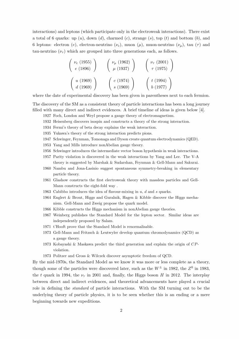
6 leptons: electron (e), electron-neutrino (νe), muon (µ), muon-neutrino (νµ), tau (τ) and
tau-neutrino (ντ ) which are grouped into three generations each, as follows.(νe (1955)
e (1896)
) (νµ (1962)
µ (1937)
) (ντ (2001)
τ (1975)
)(u (1969)
d (1969)
) (c (1974)
s (1969)
) (t (1994)
b (1977)
)where the date of experimental discovery has been given in parentheses next to each fermion.
The discovery of the SM as a consistent theory of particle interactions has been a long journey
filled with many direct and indirect evidences. A brief timeline of ideas is given below [4].
1927 Foch, London and Weyl propose a gauge theory of electromagnetism.
1932 Heisenberg discovers isospin and constructs a theory of the strong interaction.
1934 Fermi’s theory of beta decay explains the weak interaction.
1935 Yukawa’s theory of the strong interaction predicts pions.
1947 Schwinger, Feynman, Tomonaga and Dyson create quantum electrodynamics (QED).
1953 Yang and Mills introduce nonAbelian gauge theory.
1956 Schwinger introduces the intermediate vector boson hypothesis in weak interactions.
1957 Parity violation is discovered in the weak interactions by Yang and Lee. The V-A
theory is suggested by Marshak & Sudarshan, Feynman & Gell-Mann and Sakurai.
1960 Nambu and Jona-Lasinio suggest spontaneous symmetry-breaking in elementary
particle theory.
1961 Glashow constructs the first electroweak theory with massless particles and Gell-
Mann constructs the eight-fold way .
1963 Cabibbo introduces the idea of flavour-mixing in u, d and s quarks.
1964 Englert & Brout, Higgs and Guralnik, Hagen & Kibble discover the Higgs mecha-
nism. Gell-Mann and Zweig propose the quark model.
1966 Kibble constructs the Higgs mechanism in nonAbelian gauge theories.
1967 Weinberg publishes the Standard Model for the lepton sector. Similar ideas are
independently proposed by Salam.
1971 t’Hooft prove that the Standard Model is renormalisable.
1973 Gell-Mann and Fritzsch & Leutwyler develop quantum chromodynamics (QCD) as
a gauge theory.
1973 Kobayashi & Maskawa predict the third generation and explain the origin of CP -
violation.
1973 Politzer and Gross & Wilczek discover asymptotic freedom of QCD.
By the mid-1970s, the Standard Model as we know it was more or less complete as a theory,
though some of the particles were discovered later, such as the W± in 1982, the Z0 in 1983,
the t quark in 1994, the ντ in 2001 and, finally, the Higgs boson H in 2012. The interplay
between direct and indirect evidences, and theoretical advancements have played a crucial
role in defining the standard of particle interactions. With the SM turning out to be the
underlying theory of particle physics, it is to be seen whether this is an ending or a mere
beginning towards new expeditions.
2
1.2 Foundations of the Standard Model
The Standard Model of particle physics is built on the ideas of gauge invariance and sponta-
neous symmetry breaking [5–8] . The idea of gauge invariance was first discovered in classical
theory of electrodynamics, when it was realized that the different kinds of the vector potentials
Aµ, related by
Aµ → Aµ + ∂µα , (1.2.1)
could give rise to the same physical electric and magnetic fields. The above transformation on
Aµ (vector/gauge field) is known as the gauge transformation. Mathematically this amounts
to saying that the action
S =
∫d4x L = −1
4
∫d4x FµνF
µν = −1
4
∫d4x (∂µAν − ∂νAµ)2 . (1.2.2)
stays invariant under the gauge transformation in equation 1.2.1.
In quantum electrodynamics (QED), the excitation of the Aµ field corresponds to photons.
An AµAµ term is forbidden in equation 1.2.2 due to gauge invariance. Therefore, zero mass
of photons can be understood in terms of invariance of the Lagrangian under the gauge
transformations.
Now we consider the scenario where a spin-12 field (ψ) interacts with the photon field. The
Lagrangian for such a system is given as
L = −1
4FµνF
µν + iψ (∂µ − i Aµ)ψ . (1.2.3)
It can be seen that the Lagrangian is invariant under the global phase rotations of the field
ψ i.e.
ψ(x)→ eiαψ(x) , (1.2.4)
but is not invariant under the gauge transformation of the Aµ field as given in equation 1.2.1.
Since photons are observed to be massless, the theory must respect gauge invariance.
Note that if we make the transformations in equation 1.2.4 local, then for the combined
transformations
Aµ(x)→ Aµ(x) + ∂µα(x) , ψ(x)→ eiα(x)ψ(x) , (1.2.5)
the Lagrangian in equation 1.2.3 stays invariant. The continuous symmetry transformations
in equation 1.2.5 can be mapped to the U(1) Lie group, where the field ψ transforms in the
fundamental representation and Aµ transforms in the adjoint representation. The quantum
field theory of electrodynamics hence corresponds to a U(1) gauge theory. As an aside, note
that the symmetry operations in equation 1.2.5 with constant α are referred to as the global
symmetry transformations and correspond to a conserved current, Jµ and conserved charge
(Nother’s theorem).
While a successful field theory for QED existed, attempts made to formulate a coherent
quantum theory for weak interactions were less successful. The first theory was given by Fermi,
3

where the interactions were written as four-fermion operators with the operator structure same
as QED. While it fitted some of the low energy data, there were issues with unitarity and
renormalisation as the theory was really an effective theory in terms of higher dimensional
operators (dim> 4) and it failed at high energies. Since the weak interactions were observed to
be short-ranged unlike the electromagnetic interactions, it was thought that a massive gauge
particle could in principle serve as a consistent theoretical explanation at high energies. This
was the idea implemented in Intermediate Vector Boson theory, whose Lagrangian is
Lweak = −1
4WµνW
µν + iψγµ∂µψ + iψ′γµ∂µψ′ + ψγµψ′Wµ +M2
WWµWµ + h.c. . (1.2.6)
The weak interactions at that time were observed only in the charged current processes before
1970’s, as a result only massive charged gauge bosons viz., W± were postulated 1. Although
the Intermediate Vector Boson theory apparently looked renormalizable due to absence of
higher-dimensional operators, it was actually non-renormalizable at higher energies. This can
be understood by considering the W propagator,
1
q2 −M2W
(−gµν +
qµqµM2W
). (1.2.7)
This scales as 1/q2 at low energies but becomes constant at higher energies taking us back
to the same situation as the Fermi theory. The naive counting of divergences hence breaks
at higher q’s. On the other hand, if the W propagator was coupled to a conserved current
Jµ, such that qµJµ = 0, then a scaling as 1/q2 could be achieved. However, the mass term
of weak boson W in the equation 1.2.6 explicitly breaks gauge invariance and MW cannot be
set to zero because the weak interaction is short-range. The solution to write a consistent
theory for weak interactions came with the idea of spontaneous symmetry breaking (SSB) of
the gauge symmetries.
The concept of spontaneous breaking of the symmetry is quite different from that of explicit
breaking. While the symmetry of the Lagrangian is completely broken at all energy scales
for the latter case, in the former case the symmetry is broken only by the ground state of the
system but the Lagrangian still preserves the symmetry. It just gets hidden due to expansion
of the fields around the true minimum. If the symmetry transformation is described by the
unitary operator U , then SSB implies
L = ULU † , U |0〉 6= |0〉 . (1.2.8)
Note that due to Lorentz invariance, only scalar fields can aid in the phenomena of sponta-
neous symmetry breaking.
To explain the idea of SSB in detail, we consider a simplistic example of scalar field φ =ρ+ iη√
2theory, which is invariant under U(1) global transformations2.
L = ∂µφ†∂µφ+m2φ†φ− λ(φ†φ)2 . (1.2.9)
1Here the fermions ψ and ψ′ have a relative charge difference of ±1.2We will come to gauge symmetries shortly, after analyzing the repercussions of breaking a global symmetries
spontaneously.
4
Re 𝜙
Im 𝜙
V 𝜙
𝑣
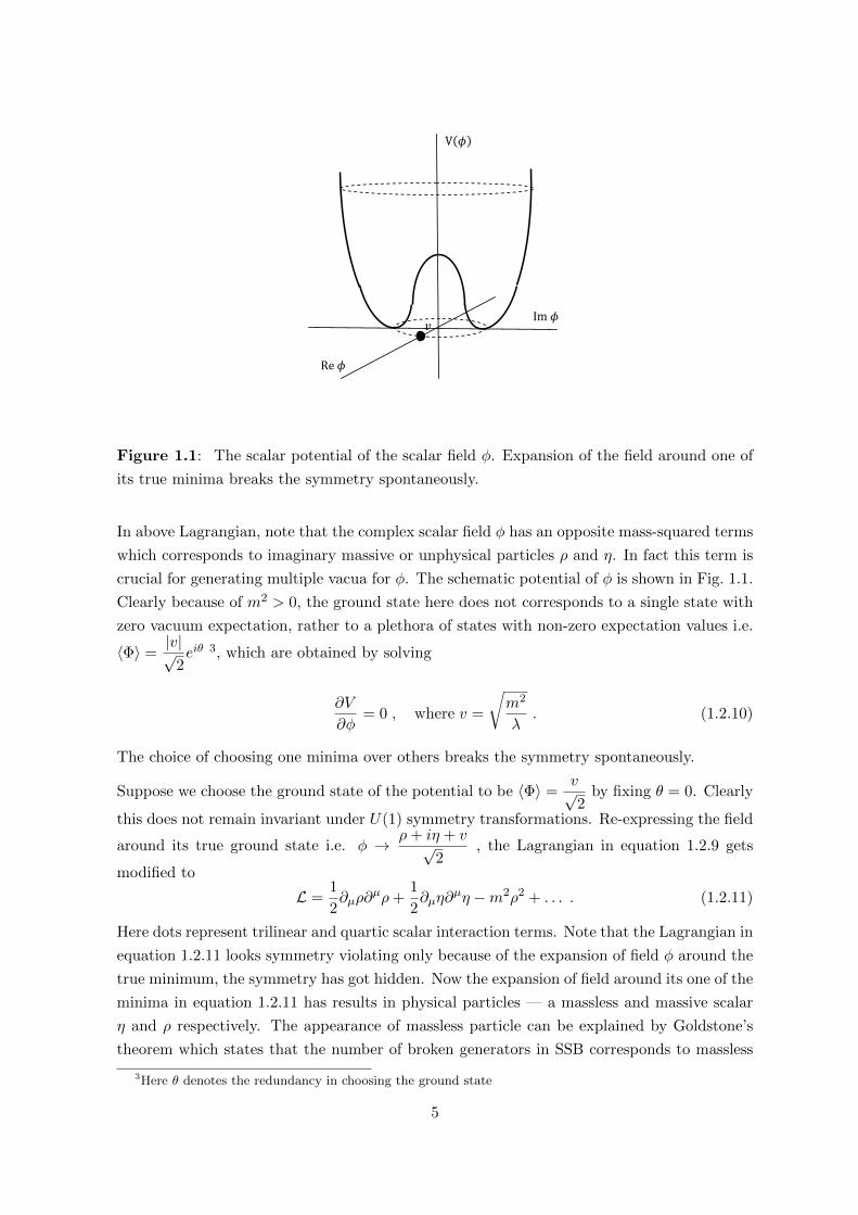
Figure 1.1: The scalar potential of the scalar field φ. Expansion of the field around one of
its true minima breaks the symmetry spontaneously.
In above Lagrangian, note that the complex scalar field φ has an opposite mass-squared terms
which corresponds to imaginary massive or unphysical particles ρ and η. In fact this term is
crucial for generating multiple vacua for φ. The schematic potential of φ is shown in Fig. 1.1.
Clearly because of m2 > 0, the ground state here does not corresponds to a single state with
zero vacuum expectation, rather to a plethora of states with non-zero expectation values i.e.
〈Φ〉 =|v|√
2eiθ 3, which are obtained by solving
∂V
∂φ= 0 , where v =
√m2
λ. (1.2.10)
The choice of choosing one minima over others breaks the symmetry spontaneously.
Suppose we choose the ground state of the potential to be 〈Φ〉 =v√2
by fixing θ = 0. Clearly
this does not remain invariant under U(1) symmetry transformations. Re-expressing the field
around its true ground state i.e. φ → ρ+ iη + v√2
, the Lagrangian in equation 1.2.9 gets
modified to
L =1
2∂µρ∂
µρ+1
2∂µη∂
µη −m2ρ2 + . . . . (1.2.11)
Here dots represent trilinear and quartic scalar interaction terms. Note that the Lagrangian in
equation 1.2.11 looks symmetry violating only because of the expansion of field φ around the
true minimum, the symmetry has got hidden. Now the expansion of field around its one of the
minima in equation 1.2.11 has results in physical particles — a massless and massive scalar
η and ρ respectively. The appearance of massless particle can be explained by Goldstone’s
theorem which states that the number of broken generators in SSB corresponds to massless
3Here θ denotes the redundancy in choosing the ground state
5
particles which are known as Goldstone bosons in literature. Any global symmetry which is
broken spontaneously will inevitably yield massless fields. However absence of these scalars
in nature put such theories into serious trouble.
Thus far we have not addressed the solution of writing consistent broken gauge theories and
have discovered a new problem of massless particles associated with spontaneous breaking of
global symmetry. It was then realized that if a local gauge symmetry is broken spontaneously
instead of a global one then the massless boson can be absorbed as the longitudinal degree of
freedom of the gauge boson. This comes under the name of Brout-Englert-Higgs mechanism [9,
10], which is popularly known as Higgs mechanism. The triumph in incorporating Higgs
mechanism is that the spontaneous broken gauge theories are renormalizable [11]. Hence one
can write massive gauge field theories in a consistent manner.
To illustrate the procedure of SSB in gauge theories, we again consider a scalar field φ but
now charged under a gauged U(1) symmetry. The Lagrangian in equation 1.2.9 now gets
modified to,
L = −1
4FµνF
µν + (∂µ − igAµ)φ†(∂µ + igAµ)φ+m2φ†φ− λ(φ†φ)2 . (1.2.12)
As before, minimizing the potential and expressing the field around its ground state results
in a massless field η and a massive degree of freedom ρ. Rewriting the above Lagrangian in
terms of new fields:
L = −1
4FµνF
µν +g2v2
2AµA
µ +1
2∂µρ∂
µρ+1
2∂µη∂
µη −m2ρ2 + gvAµ∂µη + . . . , (1.2.13)
where dots represent the trilinear and the quartic terms. Notice the bilinear term which is an
admixture of the gauge field and the massless field. The term can be interpreted as a gauge
transformation on Aµ field.
g2v2
2AµA
µ +1
2∂µη∂
µη + gvAµ∂µη → g2v2
2
(Aµ +
∂µη
gv
)2
. (1.2.14)
Hence ∂µη appears as the longitudinal degree of mode the massive gauge field. However in the
Lagrangian η field still enters in the cubic and the quatic interactions. To make the physical
particle content explicit, we write fields in the non-linear parameterization i.e.
φ =ρ+ iη + v√
2= eiη
′(ρ′ + v√
2
), (1.2.15)
where for small field expansions ρ′ ∼ ρ and η′ ∼ η. In terms of these new fields ρ′, η′ and
A′µ = Aµ +∂µηgv , the Goldstone mode disappears from the theory leaving the massive scalar
and the vector field.
L = −1
4F ′µνF
µν ′ +g2v2
2A′µA
µ′ +1
2∂µρ
′∂µρ′ −m2ρ2′ − λvρ3′ − λ
4ρ4′ . (1.2.16)
The above Lagrangian can be interpreted by the means of performing a special gauge trans-
formation viz., the unitary gauge transformation i.e.
φ(x)→ φ′(x) = e−iη′v φ =
(ρ′ + v)√2
, and Aµ → A′µ = Aµ +∂µη
gv. (1.2.17)
6
Hence our twin problems — mass of gauge bosons and massless scalar — gets solved by
invoking the spontaneous breaking of the gauge symmetry. To conclude, gauge invariance
and spontaneous symmetry breaking mechanism are powerful tools for expressing the theories
with massive gauge bosons in a consistent manner.
1.3 The Electroweak part of the Standard Model
The electroweak part of the SM is often popularly known as the Glashow-Salam-Weinberg
model. In the previous section 1.2, we had discussed that the difficulties in describing weak
interactions could be resolved if the gauge symmetry was broken spontaneously. Now the
task is to determine the underlying symmetry associated with weak interactions. To do that,
let us consider the interaction part of the Intermediate Vector Boson theory
Lintweak = ψγµψ
′Wµ . (1.3.1)
The simplest possible gauge group which we can consider to describe the weak interactions
is SU(2) with ψ and ψ′ transforming as a doublet under SU(2). Note that only left chiral
fermions4 could be charged under this SU(2) due to observation of maximum parity violation
in charged currents [12] to which V − A structure provides a good fit [13, 14]. Among the
three generators of the SU(2) group, two of them can be associated with W± i.e. the charged
current and the third one with the neutral current. Since both electromagnetism and weak
forces were mediated by spin-1 particles, there were many efforts to unify these two forces.
Note that one could not have simply considered the third generator of SU(2) with the photon
since the interactions mediated in electromagnetism were parity conserving. It was realized
that the simplest possible gauge group for electroweak unification was SU(2)L×U(1)Y . The
charges associated with U(1)Y gauge group were termed as hypercharges. Since the low energy
theory preserves U(1)em, therefore the electroweak gauge group should spontaneously break
to electromagnetism. The generator which remains conserved after the symmetry breaking is
a linear combination of T3 and hypercharge and is given as Q = T3 + Y2 .
The gauge group of the Standard Model is the direct product of strong interactions i.e. SU(3)c
and electroweak interactions i.e. SU(2)L × U(1)Y , where c, L and Y stands for colour, left
chiral and hypercharge respectively. The SU(3)c symmetry results in eight gauge bosons i.e.
the gluons and the electroweak gauge group corresponds to the four gauge bosons —Wµ1−3
for SU(2) and Bµ for U(1)Y with the gauge couplings g3, g and g′ respectively. Amongst
the matter content, there exist three generations of quarks and leptons each which are listed
in Table 1.1. The characterization of the generation is based on the mass hierarchies — the
first generation corresponds to the lightest fermions and the third generation to the heaviest5.
The conservation of SU(2)L ×U(1)Y along with Lorentz invariance not only necessitates the
4Apart from the gauge symmetries, SM Lagrangian should also be invariant under the Lorentz transfor-
mations. Correspondingly the fermionic fields in the Lagrangian can be projected onto their chiral basis
(ψ = ψL + ψR) as the chirality operator i.e. γ5 commutes with the Lorentz transformations.5However it is still not known whether the neutrinos follow the same hierarchical patterns or not.
7
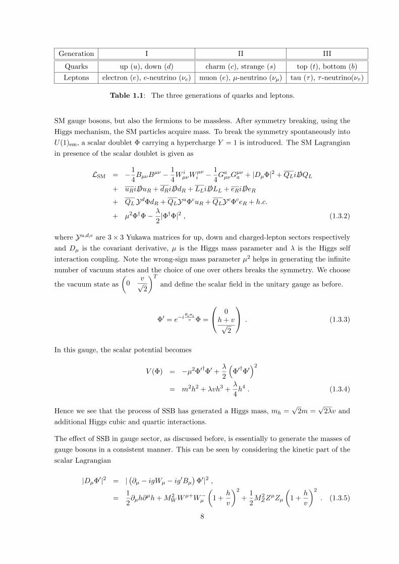
Generation I II III
Quarks up (u), down (d) charm (c), strange (s) top (t), bottom (b)
Leptons electron (e), e-neutrino (νe) muon (e), µ-neutrino (νµ) tau (τ), τ -neutrino(ντ )
Table 1.1: The three generations of quarks and leptons.
SM gauge bosons, but also the fermions to be massless. After symmetry breaking, using the
Higgs mechanism, the SM particles acquire mass. To break the symmetry spontaneously into
U(1)em, a scalar doublet Φ carrying a hypercharge Y = 1 is introduced. The SM Lagrangian
in presence of the scalar doublet is given as
LSM = −1
4BµνB
µν − 1
4W iµνW
µνi −
1
4GaµνG
µνa + |DµΦ|2 +QLi /DQL
+ uRi /DuR + dRi /DdR + LLi /DLL + eRi /DeR
+ QL YdΦdR +QLYuΦcuR +QLYeΦceR + h.c.
+ µ2Φ†Φ− λ
2|Φ†Φ|2 , (1.3.2)
where Yu,d,e are 3× 3 Yukawa matrices for up, down and charged-lepton sectors respectively
and Dµ is the covariant derivative, µ is the Higgs mass parameter and λ is the Higgs self
interaction coupling. Note the wrong-sign mass parameter µ2 helps in generating the infinite
number of vacuum states and the choice of one over others breaks the symmetry. We choose
the vacuum state as
(0
v√2
)Tand define the scalar field in the unitary gauge as before.
Φ′ = e−iθiσiv Φ =
0h+ v√
2
. (1.3.3)
In this gauge, the scalar potential becomes
V (Φ) = −µ2Φ′†Φ′ +
λ
2
(Φ′†Φ′)2
= m2h2 + λvh3 +λ
4h4 . (1.3.4)
Hence we see that the process of SSB has generated a Higgs mass, mh =√
2m =√
2λv and
additional Higgs cubic and quartic interactions.
The effect of SSB in gauge sector, as discussed before, is essentially to generate the masses of
gauge bosons in a consistent manner. This can be seen by considering the kinetic part of the
scalar Lagrangian
|DµΦ′|2 = |(∂µ − igWµ − ig′Bµ
)Φ′|2 ,
=1
2∂µh∂
µh+M2WW
µ+W−µ
(1 +
h
v
)2
+1
2M2ZZ
µZµ
(1 +
h
v
)2
. (1.3.5)
8
where,
W±µ =W1µ ± iW2µ√
2, MW =
1
2gv ,
Zµ = cos θWW3µ − sin θWBµ , MZ =1
2v
√g2 + g′2 ,
Aµ = sin θWW3µ + cos θWBµ , MA = 0 . (1.3.6)
Here θW is referred as the Weinberg angle and is given as tan θW =g′
g. Since the electroweak
symmerty gets broken to electromagnetism, the three broken generators are absorbed as
the longitudinal modes for W± and Z, the unbroken generator corresponds to the massless
photon. The masses and W and Z bosons can be expressed in terms of ρ parameter as
ρ =M2W
M2Z cos2 θW
= 1 . (1.3.7)
This parameter is exactly equal to unity at tree-level in Standard Model.
Similar to gauge bosons, Higgs mechanism also helps in generating the mass terms of the SM
fermions. Let us consider the Yukawa part of the Lagrangian viz.,
LYuk = QiL YdijΦdjR +QiLYuijΦcujR +QiLYeijΦcejR + h.c.
= uLMu
(1 +
h
v
)uR + dLMd
(1 +
h
v
)dR + `LM`
(1 +
h
v
)`R + h.c. . (1.3.8)
The Yukawa matrices Y’s are in general non-diagonal and non-hermition. They are diagonal-
ized by performing bi-unitary transformations i.e.
Mu =v√2V †uLYuVuR , Md =
v√2V †dLYdVdR , M` =
v√2V †`LY`V`R . (1.3.9)
Here V ’s are the rotation matrices, Mu = diag(mu,mc,mt), Md = diag(md,ms,mb) and
M` = diag(me,mµ,mτ ). Note that the absence of right handed neutrinos lead to massless
neutrinos in Standard Model framework. The above mass diagonalization modifies the struc-
ture of interactions of gauge bosons with fermions and leads to flavour changing interactions
in charged currents mediated by W
Lcc =g√2uiγ
µPL[VCKM]ijdj W+µ + h.c. , (1.3.10)
where VCKM = V †uLVdL. Note that the flavour changing matrix VCKM is also unitary and can
be described in terms of nine parameters — three rotation angles and six complex phases. Out
of these six phases, five can be absorbed by the rotation of the quark fields. The remaining
phase is the sole source of CP violation in weak interactions.
In contrast with the charged current, flavour changing interactions mediated by Z and γ are
absent at the tree-level because charges of all same-type fermions under U(1)Y symmetry are
same. The Lagrangian corresponding to the neutral current interactions is given as
Lnc = efγµf Aµ +g
cos θW
(gfLfγ
µPLf + gfRfγµPRf
)Zµ , (1.3.11)
9
where, ef is the electromagnetic charge of the fermion f , T3 is the isospin of the fermion and
gfL,R = T3 − ef sin2 θW . The electromagnetic charge of electron gets related to the SU(2)L
gauge coupling g as e = g sin θW .
To conclude this section, we highlight the major predictions and findings of the electroweak
sector of the Standard Model:
1. Unification of electromagnetism and weak forces via the electroweak gauge group SU(2)L×U(1)Y . This is the minimal symmetry which would give rise to such a unification at
high scales.
2. The electroweak theory predicts the presence of new kind of neutral currents coupling
to heavy gauge boson, Z.
3. The electroweak structure along with three generations of fermions naturally incorpo-
rates the phenomena of CP violation.
4. Standard Model predicts ρ parameter to be exactly equal to unity at the classical level,
with very small quantum corrections.
1.4 Current status of the SM
In the previous section, we considered the electroweak sector of the Standard Model. Due to
its specific gauge group i.e. SU(2)L×U(1)Y definite interaction form exist between particles.
Over past several years, these forms have been tested to a great degree of accuracy at electron-
positron (LEP, SLAC, Belle, Babar), proton-antiproton (UA1, UA2, Tevatron), electron-
proton (HERA) and proton-proton (LHC) colliders. The gauge sector was the first to be
established with the discovery of W± and Z bosons at UA1 and UA2 [15, 16] followed by
precision measurements of gauge boson interactions with fermions and self interactions at
LEP-I, LEP-II and SLAC, where some of the interactions were tested upto a 0.1% level [17,
18]. The flavour sector has also been established at the B-factories by BABAR and BELLE
collaborations [19].
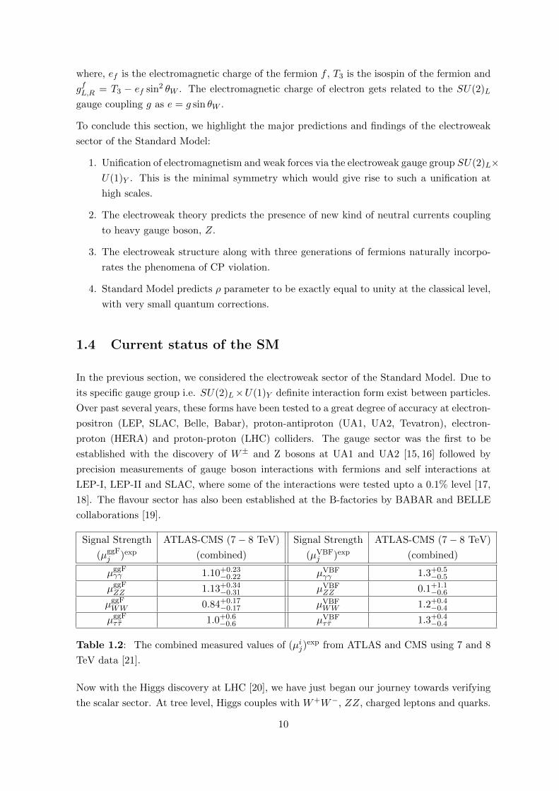
Signal Strength ATLAS-CMS (7− 8 TeV) Signal Strength ATLAS-CMS (7− 8 TeV)
(µggFj )exp (combined) (µVBF
j )exp (combined)
µggFγγ 1.10+0.23
−0.22 µVBFγγ 1.3+0.5
−0.5
µggFZZ 1.13+0.34
−0.31 µVBFZZ 0.1+1.1
−0.6
µggFWW 0.84+0.17
−0.17 µVBFWW 1.2+0.4
−0.4
µggFτ τ 1.0+0.6
−0.6 µVBFτ τ 1.3+0.4
−0.4
Table 1.2: The combined measured values of (µij)exp from ATLAS and CMS using 7 and 8
TeV data [21].
Now with the Higgs discovery at LHC [20], we have just began our journey towards verifying
the scalar sector. At tree level, Higgs couples with W+W−, ZZ, charged leptons and quarks.
10
Due to its dominant coupling with top, it couples with gg and γγ6 at one loop. The Higgs can
be produced at the LHC via gluon fusion (ggF), vector-boson fusion (VBF), and in association
with SM gauge bosons (Vh), as well as with a top pair (tth) and it can decay to γγ, ZZ∗ →`+`−`′+`′−, WW ∗ → `+ν``
′−ν ′`, ff if (mh > mf/2). The accurate measurements of these
couplings will hold a clues about the scalar sector and the nature of electroweak symmetry
breaking. Table 1.2 shows combined ATLAS and CMS signal strengths measurements from
run-I data for the observed Higgs Boson into various channels [21]. Although the uncertainties
in measurements at the present moment are large O(10 − 20%), we can clearly see that the
SM is compatible with the data. Other Higgs couplings for instance the tri-linear and quartic
at present are extracted using the information of the Higgs mass and the vacuum expectation
value. Its independent measurement is yet to be made at the experiments and this will
provide us a clear understanding of the nature of the electroweak symmetry breaking that
whether it occurs because of a Higgs doublet or many more. Apart from Higgs studies, LHC
is also actively probing other sectors and so-far have found no significant deviations from the
Standard Model predictions, see for example [22].
Despite such phenomenal success of the SM, there are several reasons to believe the existence
of the physics beyond Standard Model [23, 24]. The Higgs mass is thought to be one of the
major reasons for existence of physics beyond Standard Model because it is unstable in the
presence of new particles at scales much higher than the electroweak scales. Suppose a new
particle is present scale Λ >> OEW, then corrections to Higgs mass scales as
δm2h ∝ Λ2 . (1.4.1)
To arrange mh ≈ 125 GeV then requires large amount of fine tuning. The Higgs mass
correction sets the scale of new physics to be roughly around a TeV to avoid large fine tuned
cancellations. This problem is primarily associated with the fundamental scalars and do not
arise for fundamental fermions and gauge particles. This can be simply understood based on
symmetry arguments. If we have a theory with only fundamental fermions and no scalars,
then the fermionic mass term viz., ψψ is symmetric under U(1)V transformations. In the
limit of zero mass, there is an enhanced symmetry of the theory i.e. the chiral symmetry
U(1)A. If this symmetry is also preserved by the quantum fluctuations, then fermion remains
massless even after performing higher order calculations. Notice this a phenomenal result
because this implies that in presence of m 6= 0, the mass corrections are proportional to the
symmetry breaking term which is m itself. The same result holds true for the gauge bosons.
The gauge symmetry principles prevent the masses of gauge bosons from becoming too large.
This is remarkable result in itself because the chiral/gauge symmetry argument prevents the
fermions/gauge bosons mass term becoming dependent on the cut off scale. Notice that we
cannot use such arguments of the SM Higgs. The mass term which arises from Φ†Φ interaction
is already invariant under all global and gauged symmetries. Therefore M2h by no means is
protected by any enhanced symmetry of the theory. It might still happen that due to fine
tuned Higgs bare mass parameter, the actual mass of Higgs may be light and doesn’t depend
6Here the coupling with W+W− also plays a crucial role
11
on the cut-off scale. But we strongly believe that just like fermions and gauge bosons, there
may be some phenomena which prevents Higgs boson mass. There is also a counter-view that
the issue associated with the stability of the mass of the fundamental scalar is more-or-less
aesthetic and should be taken with a pinch of salt.
There have been numerous attempts to solve the Higgs hierarchy or rather fine tuning prob-
lem [25]. The most popular one has undoubtedly been supersymmetry, where there is an
additional symmetry which relates the fermionic degree of freedom with the bosonic ones.
Here the chiral symmetry of fermions protects the mass of the fundamental scalars. Alter-
natively, there are composite Higgs models, where Higgs is not a fundamental scalar but a
bound state of fermions which are charged under a new gauge interaction similar to QCD.
Therefore the problem associated with the elementary scalar at first place only doesn’t arise.
If the observed Higgs mass is protected by symmetry arguments then new particles should
appear at the TeV-scale. But the continuous running of LHC has resulted in no sign of new
particle at the TeV-scale. This has put the idea of naturalness and fine tuning into trouble
and has resulted in a new problem of little hierarchy [26]. Experiments suggest that NP
scales should atleast be greater than 2-3 TeV and for some models even 5 TeV, while Higgs
mass stablization requires the scales to be present at a TeV. In the light of this, alternate
models with the concept of neutral naturalness viz., where new particles do not have strong
interactions have been hypothesized. Time will only tell that which of these models or any
other variant of these models will survive.
Another issue which concerns Standard Model is the existence of the neutrino oscillations [27,
28]. The massless neutrinos in SM could not have given rise to this phenomenon. The
problem may be easily alleviated by adding three right handed neutrinos and generating
masses through Higgs mechanism, but the zero charge of neutrinos creates a dilemma over
origin of neutrino masses. The fermions uncharged under electromagnetism are either Dirac-
like or Majorana-like and the process of acquiring mass is completely different for the two
cases. While Higgs mechanism works well with the Dirac-neutrinos, see-saw mechanism has
been suggested as an alternative method for origin of mass for Majorana-like neutrinos. The
data on the neutrino oscillation does hint towards new physics, but leaves its nature to be
completely unknown.
Astronomically there are many compelling evidences of the existence of dark matter ranging
from the proper velocities of galaxies clusters, rotation curve measurements of the galaxies,
Cosmic Microwave Background Radiation etc [29]. However till date no interactions other
than the gravitational ones have been reported for these particles. Attempts have been made
in the past to determine the particle content of dark matter but all efforts so far have gone
in vain. Since the existence of dark matter cannot be denied, some new physics should hold
the explanation to this mystery.
There are few other aesthetic problems associated with the SM viz., why do we have SU(3)c×SU(2)L×U(1)Y gauge symmetry, why there are three generations of fermions and one Higgs
doublet, why is the mass of an electron and top so different from each other?
12

These are few problems which have intrigued the theorist time and again. While there have
been many theoretical breakthrough ideas as previously mentioned like supersymmetry, com-
posite Higgs, extra dimensions which attempt to address some of the above problems, none
of them have yet shown any observable effect at the detectors.
At present, SM fits the data well but it certainly cannot be the complete picture till all
scales because around Planck scale the gravitational effects become strong and such effects
would then have to be included in a consistent manner. Since data seems to be in agreement
with the Standard Model predictions within the experimental uncertainties, the new physics
may be either hidden under the large Standard Model backgrounds or may be present in
an inaccessible part of the parameter space. Given the scenario where no model is being
favoured by the experiments we choose to take an alternative and simplistic approach which
we describe in detail in the next chapter.
13
Chapter 2
Small Expeditions out of the Standard Way
Experimental searches for physics beyond the Standard Model have – till date – yielded
neither significant positive results nor specific directions or paths to follow. However it is
clear from the discussions in the previous chapter, that physics beyond the Standard Model
must exist. In the absence of any specific hint about the nature of new physics, various new
physics models are current, and all being consistent with the present data, make the search
strategies somewhat incoherent. Wide-reaching ideas encompassing all of particle physics,
such as compositeness, supersymmetry or extra dimensions belong to this class, and one has
only to look at the number of papers predicting signals for these to see the huge variety of
possibilities which experimental physicists have to confront.
In such a situation, focused studies – often data-driven – have become extremely important.
Thus, simple extensions of the Standard Model and effective field theories are being increas-
ingly favoured to analyze the effects of new physics in data, as they have a small number of
free parameters and hence greater predictivity. Similarly, one looks at simplified versions of
the deeper models mentioned above where only a small sector of the full theory is relevant. In
general, data can provide direct or indirect hints for the presence of new physics, depending
upon its nature. For example, while the lighter particles may be observed directly as reso-
nances in the invariant mass spectrum, such a method would not work for heavier resonances
due to limited statistics. One would then have to rely upon the indirect clues where the
presence of such a heavier resonance could lead to deviations in well measured/predictable
observables.
The above approach has been adapted in this thesis work, wherein simple extensions of the
Standard Model have been considered to probe and predict direct and indirect hints in the
data. Our aim is not to address the problems listed in chapter 1 in a top-down fashion, but
rather to understand the data and eventually make predictions in a bottom-up approach.
The hope is that such studies would eventually guide us towards the UV-complete models,
at some stage in future. We have, thus, chosen a few select areas, focussing on extensions
of the Standard Model where extra bosons or additional couplings of the existing bosons are
involved.
14
Recent flavour measurements in the neutral B decays concerning b to s flavour transitions [30–
33] have hinted towards lepton flavour-universality violation. Although the individual devi-
ations from the SM predictions are not more than 2-3σ, what is intriguing is the fact that
so many observables are simultaneously pointing towards the need of a similar kind of new
physics. Part of the thesis work has been devoted towards exploring a possible new physics
explanation for a few of the above anomalies. In chapter. 3, we have presented the simulta-
neous solutions to the anomaly RK and neutrino mixings. A class of U(1)X lepton flavour
universality violating models have been identified in a bottom-up approach. Our solutions
are consistent with the P ′5 anomaly. At the time when the work was done, results for the
RK∗ anomaly did not exist. We also analyze the implications of including RK∗ measurements
towards end of chapter. 3.
The indirect effect of new physics may also affect the gauge boson self interactions. In another
such study discussed in chapter 4, we perform a dedicated collider analysis for the process
pp→Wγ → `ν`γ, to study the new physics effects manifesting in the presence of anomalous
WWγ couplings. Instead of using the standard conventional variable i.e. the transverse
momentum of the photon, we identify other kinematic variables which aid in better signal
sensitivities.
The diphoton channel is perhaps one of the cleanest probes for searching for new physics at the
LHC – witness the discovery of the Higgs Boson [20]. Owing to better signal and background
distinctions, the sensitivity of these channels to detect new physics is much higher than that
of other channels like bb or τ τ . In chapter 5, we study the direct detection prospects of a
light scalar (lighter than the Higgs Boson) in the di-photon channel in the context of a type-I
2HDM and find favourable regions where such a light scalar could be probed with the current
luminosities at the LHC. We also briefly discuss the light scalar decays to bb final states.
The discovery of a diphoton resonance at the LHC would prompt various questions, which
would hold true for any heavy resonance particle, e.g. does a heavy mass resonance corre-
sponds to a two-photon final state or could that be an artefact of a multiphoton (three or
more) final state appearing as an apparent diphoton state? or, what would be the spin of
such a prototype resonance? We have attempted to address these questions in chapter 6 using
an effective field theory approach in the context of a spin-0, spin-1 and spin-2 resonances. In
fact, a couple of years back, an anomaly in the diphoton invariant mass around 750 GeV had
been announced simultaneously by both ATLAS and CMS collaborations. Of course, it is
well known that the anomaly disappeared with increased statistics [34,35].
Most of the problems described above have been addressed by minimally extending the SM by,
for example, (i) the addition of singlet scalars, (ii) SU(2)L doublet scalars, (iii) right handed
neutrinos, (iv) additional gauge symmetries, (v) higher-dimensional operators. or some com-
binations of these. We describe the theoretical framework of these minimal extensions in the
following sections.
15
2.1 Singlet Scalars
Introducing additional scalars S, uncharged under the SM gauge group, is perhaps the mini-
mal way of going beyond the SM [36]. Such extensions are useful in explaining various prob-
lems, such as dark matter, smallness of neutrino mass masses through see-saw mechanism
in presence of three right handed neutrinos, strong CP-problem, fermionic mass hierarchy
through the Froggatt-Nielson mechanism, µ problem of supersymmetry and many more. The
new SM-singlet scalar may be either charged under a Z2 symmetry or some additional gauge
symmetry depending upon the nature of the problem in consideration.
Let us consider two real scalar SM singlet fields S1 and S2 which transform under Z2 and Z ′2symmetry operations respectively. The SM fields are not affected by these transformations.
We choose to break Z2 at scale vS1 spontaneously and preserve Z ′2 at all scales. To see
the phenomenological consequences of this choice, consider the modified Higgs potential in
presence of S1 and S2 fields
V (Φ, S1, S2) = −m2Φ†.Φ + λ(
Φ†.Φ)2
+m21S
21 + λS1S
41
−m22S
22 + λS2S
42 + λΦS1S
21
(Φ†.Φ
)+λΦS2S
22
(Φ†.Φ
)+ λS1S2S
21S
22 (2.1.1)
The spontaneous breaking of Φ and S1 generates mixing between the the SM-Higgs and this
new scalar. The observed Higgs hence is an admixture of the scalars h and S1. The mixing
between them is given by
L = m2hh
2 +m2S1S2
1 + λΦS1 vEW vS1 hS1 (2.1.2)
Estimating orders of magnitude, mh ≈ O(vEW ) and mS1 ≈ O(vs1). Hence the mixing matrix
becomes (v2EW λΦS1 vEW vS1
λΦS1 vEW vS1 v2S1
)(2.1.3)
In the limit when the symmetry Z2 is broken at scales much larger than the electroweak scale,
the eigenvalues are v2S1
and v2EW
(1− λ2
ΦS1
)and the mixing angle is
vEWvS1
λΦS1 . We want λΦS1
to be at-least less than unity, such that Higgs mass remains of the order of electro-weak scale.
Consequently the mixing angle generated is small. Nevertheless this mixing leads to the
singlet scalar coupling with the SM particles. If mass of S1 is of the order of TeV scale, then
it could in principle be observed as a resonance at LHC provided its couplings are reasonable
enough.
Howsoever simple this addition of SM scalar singlet S1 may appear, it has rather powerful
implications. In this thesis, we have studied the implications of adding such a scalar in the
context of neutrino masses. The other scalar S2 on the other hand doesn’t mix with any other
scalar field and is a stable particle due to preserved Z ′2 symmetry. This could be a candidate
for the unexplained dark matter content of the Universe.
16
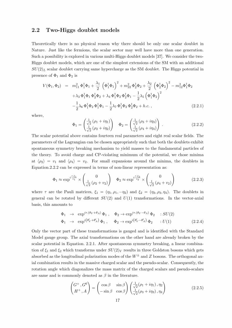
2.2 Two-Higgs doublet models
Theoretically there is no physical reason why there should be only one scalar doublet in
Nature. Just like the fermions, the scalar sector may well have more than one generation.
Such a possibility is explored in various multi-Higgs doublet models [37]. We consider the two-
Higgs doublet models, which are one of the simplest extensions of the SM with an additional
SU(2)L scalar doublet carrying same hypercharge as the SM doublet. The Higgs potential in
presence of Φ1 and Φ2 is
V (Φ1,Φ2) = m211 Φ†1Φ1 +
λ1
2
(Φ†1Φ1
)2+m2
22 Φ†2Φ2 +λ2
2
(Φ†2Φ2
)2−m2
12Φ†1Φ2
+λ3 Φ†1Φ1 Φ†2Φ2 + λ4 Φ†1Φ2 Φ†2Φ1 −1
2λ5
(Φ†1Φ2
)2
−1
2λ6 Φ†1Φ2 Φ†1Φ1 −
1
2λ7 Φ†1Φ2 Φ†2Φ2 + h.c. , (2.2.1)
where,
Φ1 =
(1√2
(ρ1 + iη1)1√2
(ρ2 + iη2)
)Φ2 =
(1√2
(ρ3 + iη3)1√2
(ρ4 + iη4)
). (2.2.2)
The scalar potential above contains fourteen real parameters and eight real scalar fields. The
parameters of the Lagrangian can be chosen appropriately such that both the doublets exhibit
spontaneous symmetry breaking mechanism to yield masses to the fundamental particles of
the theory. To avoid charge and CP-violating minimum of the potential, we chose minima
at 〈ρ2〉 = v1 and 〈ρ4〉 = v2. For small expansions around the minima, the doublets in
Equation.2.2.2 can be expressed in terms of non-linear representation as:
Φ1 ≈ expiτ.ξ1v1 ×
(0
1√2
(ρ2 + v2)
)Φ2 ≈ exp
iτ.ξ2v2 ×
(0
1√2
(ρ4 + v2)
)(2.2.3)
where τ are the Pauli matrices, ξ1 = (η1, ρ1,−η2) and ξ2 = (η3, ρ3, η4). The doublets in
general can be rotated by different SU(2) and U(1) transformations. In the vector-axial
basis, this amounts to
Φ1 → expiτ.(θV +θA) Φ1 , Φ2 → expiτ.(θV −θA) Φ2 : SU(2)
Φ1 → expi(θ′V +θ′A) Φ1 , Φ2 → expi(θ
′V −θ
′A) Φ2 : U(1) (2.2.4)
Only the vector part of these transformations is gauged and is identified with the Standard
Model gauge group. The axial transformations on the other hand are already broken by the
scalar potential in Equation. 2.2.1. After spontaneous symmetry breaking, a linear combina-
tion of ξ1 and ξ2 which transforms under SU(2)V results in three Goldston bosons which gets
absorbed as the longitudinal polarization modes of the W± and Z bosons. The orthogonal ax-
ial combination results in the massive charged scalar and the pseudo-scalar. Consequently, the
rotation angle which diagonalizes the mass matrix of the charged scalars and pseudo-scalars
are same and is commonly denoted as β in the literature.(G+ , G0
H+ , A
)=
(cosβ sinβ
− sinβ cosβ
)(1√2(ρ1 + iη1) , η2
1√2(ρ3 + iη3) , η4
)(2.2.5)
17
The masses of the charged scalar and the pseudoscalar are proportional to the terms in the
scalar potential breaking SU(2)A and U(1)A symmetry respectively. The diagonalisation
process of the neutral CP-even scalars on the other hand is independent and corresponds to
the rotation angle α. (h
H
)=
(sinα − cosα
− cosα − sinα
)(ρ2
ρ4
)(2.2.6)
Summarizing, the spontaneous breaking of the electroweak symmetry, SU(2)L × U(1)Y to
the U(1)em, results in five physical scalar fields viz. light CP-even Higgs (h), Heavy CP-even
Higgs (H), a pseudoscalar (A) and charged Higgs bosons (H±) and three Goldstone fields —
G± and G0, which gets absorbed as the longitudinal modes for the W± and the Z boson in
the unitary gauge. Expressing the doublets in terms of the physical degrees of freedom:
Φ1 =
(G+ cosβ −H+ sinβ
1√2
[h sinα−H cosα+ i (G cosβ −A sinβ) + v1]
),
Φ2 =
(G+ sinβ +H+ cosβ
1√2
[−h cosα−H sinα+ i (G sinβ +A cosβ) + v2]
), (2.2.7)
In this setup, the most general Yukawa interactions are given as
LYuk = QiL
(Yd1 ijΦ1 + Yd2 ijΦ2
)djR +QiL
(Yu1 ijΦc
1 + Yu2 ijΦc2
)ujR
+ QiL(Ye1 ijΦc
1 + Ye2 ijΦc2
)ejR + h.c. . (2.2.8)
This structure of couplings results in tree-level flavour changing neutral and charged currents
mediated by the scalars since diagonalization of Y1 and Y2 matrices is different. To illustrate
the point, we consider the Yuwaka interactions for down-type quarks:
LYuk =v√2dL
(Yd1 cosβ + Yd2 sinβ
)dR
+1√2dL
(Yd1 sinα− Yd2 cosα
)h dR
− 1√2dL
(Yd1 cosα+ Yd2 sinα
)H dR
+i√2dL
(Yd1 sinβ − Yd2 cosβ
)AdR (2.2.9)
The above interactions are written in the flavour basis. Diagonalizing the Yukawa matrices
by bi-unitary transformations VdL and VdR
Md =v√2V †dL
(Yd1 cosβ + Yd2 sinβ
)VdR , (2.2.10)
we can re-express the scalar interactions in the mass basis as
LYuk =sinα
cosβdL (Md/v) dR h−
1√2
cos(β − α)
cosβdL V
†dLYd2 VdR dR h
− cosα
cosβdL (Md/v) dRH +
1√2
sin(β − α)
cosβdL V
†dLYd2 VdR dRH
+ i tanβ dL (Md/v) dRA− i1√2
1
cosβdL V
†dLYd2 VdR dRA (2.2.11)
18
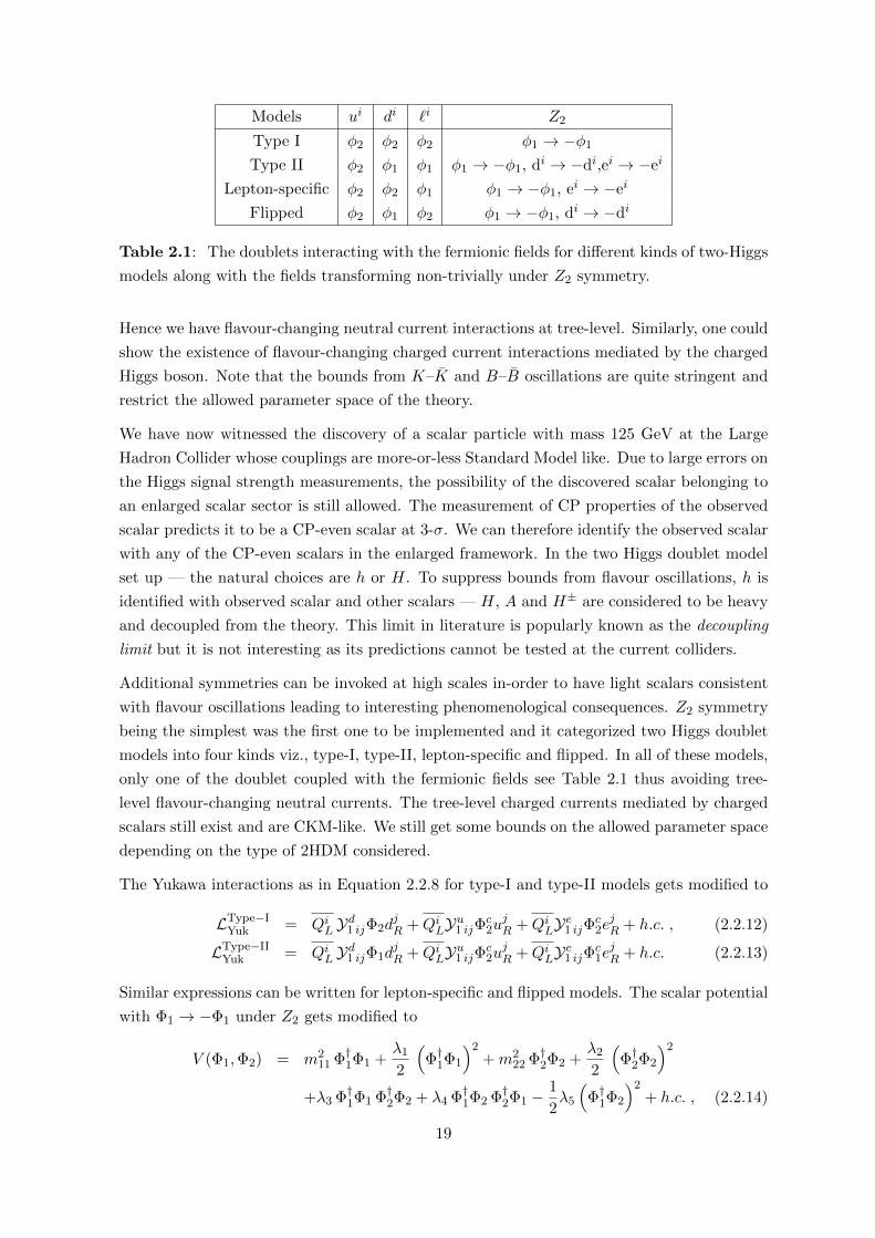
Models ui di `i Z2
Type I φ2 φ2 φ2 φ1 → −φ1
Type II φ2 φ1 φ1 φ1 → −φ1, di → −di,ei → −ei
Lepton-specific φ2 φ2 φ1 φ1 → −φ1, ei → −ei
Flipped φ2 φ1 φ2 φ1 → −φ1, di → −di
Table 2.1: The doublets interacting with the fermionic fields for different kinds of two-Higgs
models along with the fields transforming non-trivially under Z2 symmetry.
Hence we have flavour-changing neutral current interactions at tree-level. Similarly, one could
show the existence of flavour-changing charged current interactions mediated by the charged
Higgs boson. Note that the bounds from K–K and B–B oscillations are quite stringent and
restrict the allowed parameter space of the theory.
We have now witnessed the discovery of a scalar particle with mass 125 GeV at the Large
Hadron Collider whose couplings are more-or-less Standard Model like. Due to large errors on
the Higgs signal strength measurements, the possibility of the discovered scalar belonging to
an enlarged scalar sector is still allowed. The measurement of CP properties of the observed
scalar predicts it to be a CP-even scalar at 3-σ. We can therefore identify the observed scalar
with any of the CP-even scalars in the enlarged framework. In the two Higgs doublet model
set up — the natural choices are h or H. To suppress bounds from flavour oscillations, h is
identified with observed scalar and other scalars — H, A and H± are considered to be heavy
and decoupled from the theory. This limit in literature is popularly known as the decoupling
limit but it is not interesting as its predictions cannot be tested at the current colliders.
Additional symmetries can be invoked at high scales in-order to have light scalars consistent
with flavour oscillations leading to interesting phenomenological consequences. Z2 symmetry
being the simplest was the first one to be implemented and it categorized two Higgs doublet
models into four kinds viz., type-I, type-II, lepton-specific and flipped. In all of these models,
only one of the doublet coupled with the fermionic fields see Table 2.1 thus avoiding tree-
level flavour-changing neutral currents. The tree-level charged currents mediated by charged
scalars still exist and are CKM-like. We still get some bounds on the allowed parameter space
depending on the type of 2HDM considered.
The Yukawa interactions as in Equation 2.2.8 for type-I and type-II models gets modified to
LType−IYuk = QiL Yd1 ijΦ2d
jR +QiLYu1 ijΦc
2ujR +QiLYe1 ijΦc
2ejR + h.c. , (2.2.12)
LType−IIYuk = QiL Yd1 ijΦ1d
jR +QiLYu1 ijΦc
2ujR +QiLYe1 ijΦc
1ejR + h.c. (2.2.13)
Similar expressions can be written for lepton-specific and flipped models. The scalar potential
with Φ1 → −Φ1 under Z2 gets modified to
V (Φ1,Φ2) = m211 Φ†1Φ1 +
λ1
2
(Φ†1Φ1
)2+m2
22 Φ†2Φ2 +λ2
2
(Φ†2Φ2
)2
+λ3 Φ†1Φ1 Φ†2Φ2 + λ4 Φ†1Φ2 Φ†2Φ1 −1
2λ5
(Φ†1Φ2
)2+ h.c. , (2.2.14)
19
which is same for the four types of the two Higgs doublet models listed in the Table. 2.1. Type-
I model is more like the standard model as only one doublet has non-zero Yukawa coupling
and Type-II 2HDM is similar to the supersymmetric extension of the standard model. In
general there could be various other kinds of two Higgs doublet models like inert two Higgs
doublet models, BGL models etc. which have slightly different phenomenology.
In one of the chapters 6, type-I 2HDM is considered for the analysis. There the phenomenology
of a scalar h lighter than the observed scalar identified with H, in the mass range 70-110 GeV
is discussed. In another chapter 3, a different kind of 2HDM is analysed, where the two
doublets are charged differently under the abelian U(1)X symmetry. Since the motivation
of the work was to explain the RK anomaly using a Z ′, the additional scalars apart from
the observed Higgs were considered to be heavy and hence decoupled from the theory. The
additional doublet here helps to generate the correct structure of the CKM matrix, which
otherwise would have been impossible owing to non-universal X-charge assignments of the
quarks under U(1)x
2.3 Additional U(1)X gauge symmetry
In this section, we study the implications of minimally extending the SM gauge group by an
additional gauge symmetry U(1)X [38]. This addition results in a kinetic mixing between Bµ
and Xµ fields. The gauge kinetic term in this set up gets modified as
Lkin = −1
4BµνB
µν − 1
4XµνX
µν − k
2BµνX
µν , (2.3.1)
where k is the mixing strength between the two fields. The fields at present are not canonically
normalized, and could be brought to their canonical basis by following transformation,
(Bµ
Xµ
)= P
(Bµ
Xµ
), where P =
1 − k√1− k2
01√
1− k2
. (2.3.2)
In the new basis, the kinetic term in Equation. 2.3.1 becomes
Lkin = −1
4BµνB
µν − 1
4XµνX
µν . (2.3.3)
The transformations in Equation. 2.3.2 changes the neutral current structure of the fields as
follows
g Jµ3 W3µ + gY JµY Bµ + gXJ
µXXµ → g Jµ3 W3µ + gY J
µYBµ
+
(gX√
1− k2JµX −
k√1− k2
gY JµY
)Xµ (2.3.4)
We note that the redefinition of fields at this stage has changed only the current structure of
the U(1)X field.
20
Since the low energy symmetry of the nature is U(1)em, therefore the U(1)X symmetry cannot
remain conserved at all energy scales. If the SM particles, specifically quarks and leptons,
are charged under this symmetry, then the bounds from LHC on mass of X can be quite
stringent, typically around O(TeV ). In such cases, the typical scales chosen to break U(1)X
symmetry are much larger than the electroweak scale.
Another issue which concerns the X mass and more importantly Z–X mixing is the question
whether the SM Higgs doublet or any additional doublet if any, are charged under U(1)X
symmetry. If doublets transform as singlets under the action of U(1)X , then there will not
be any mass mixing between Z and X bosons and the kinetic mixing parameter k practically
remains unconstrained. However, in presence of mass mixing, k will be constrained from
various precision measurements at the LEP and the flavour factories. For example, let us
consider the case where the SM Higgs Boson and an additional scalar S, carries equal charges,
aX (for simplicity) under U(1)X symmetry. The part of the Lagrangian containing the mass
terms for the neutral gauge bosons can be given as:
Lmass = Φ†.(g
2W3µσ3 +
gY2Bµ + aX gXXµ
)×(g
2W3µσ3 +
gY2Bµ + aX gXXµ
).Φ + a2
Xg2XXµZ
′µS†S . (2.3.5)
After spontaneous symmetry breaking the true minimum of the fields correspond to 〈Φ〉 =v√2
, and 〈S〉 =vs√
2. Redefining aX gX → gX , the Lagrangian in Equation. 2.3.5 can be
written in a compact notation,
Lmass =1
2
(W3µ Bµ Xµ
)M2V
Wµ3
Bµ
Xµ
, (2.3.6)
where
M2V =
14 g
2v2 −14 g gY v
2 −12 g gXv
2
−14 g gY v
2 14 g
2Y v
2 12 gY gXv
2
−12 g gXv
2 12 gY gXv
2 g2X
(v2S + v2
) (2.3.7)
This mass matrix doesn’t account for the kinetic mixing. Incorporating the kinetic mixing
will result in
Lmass =1
2
(W3µ Bµ Xµ
)P T .M2
V .P
Wµ3
Bµ
Xµ
, (2.3.8)
where matrix P is defined in eqn 2.3.2.
We first diagonalize the 1-2 component of the above mass matrix i.e. W3µ and Bµ field to
obtain massive Zµ and massless Aµ fields,Zµ
Aµ
Xµ
=
cos θW − sin θW 0
sin θW cos θW 0
0 0 1
W
µ3
Bµ
Xµ
(2.3.9)
21
where, tan θW = gYg . The mass matrix after this rotation is given as
(Zµ Aµ Xµ
)M2Z 0 ∆
0 0 0
∆ 0 M2X
Z
µ
Aµ
Xµ
(2.3.10)
where,
M2Z =
1
4(g2 + g2
Y )v2
M2X =
g2X
1− k2
(v2S + v2
)+
g2Y v
2k2
4(1− k2)− gY gXkv
2
1− k2(2.3.11)
∆ = −gX
√g2 + g2
Y v2
2√
1− k2+kgY
√g2 + g2
Y v2
4√
1− k2(2.3.12)
and the Z–X mixing angle which diagonalizes the above mass matrix is given as
tan 2θZX =2∆
M2X −M2
Z
(2.3.13)
The mixing is stringently constrained by the Z-pole measurements at LEP and SLC; therefore
we can approximate it to be
θZX ≈∆
M2X −M2
Z
. (2.3.14)
The vacuum expectation values satisfying vs � vew, renders small mixing angles naturally.
The mass eigenstates of Z and X after mixing are given as
Zm = Z − θZXX , Z ′m = X + θZXZ . (2.3.15)
The current in Equation. 2.3.4 gets modified to,
e Jemµ Aµ +
[g
cos θW− θZX
(gX√
1− k2JµX −
k√1− k2
gY JµY
)]Zµ
+
[(gX√
1− k2JµX −
k√1− k2
gY JµY
)+ θZX
g
cos θW
]Z ′µ , (2.3.16)
where the superscript m is not written explicitly. The modifications in the current structure
of Z boson, stringently constrains θZX and k for a given value of gX . The Z-pole observables
will not only receive constraints due to the Z–X mixing, but will also be affected by the loop
effects mediated by X. However for O(TeV) scale Z ′, these effects are naturally small.
Another issue which concerns the additional gauge symmetry is anomalies. However if the
fermions are assigned vector-like charges under U(1)X , then the gauge symmetry by definition
is anomaly free. Otherwise the X-charges of the new fermionic fields should be such that the
anomaly coefficients are zero.
An additional U(1)X extension forms the backbone of the analysis reported in chapter 3.
22
2.4 Effective field theory
Effective field theory is a framework considering only those degrees of freedom which are
relevant to the energy scales in the chosen problems [39]. For instance, for solving the hydrogen
atom problem, we need not worry about the existence of quarks and similarly in the theory of
weak interactions at low scales i.e. the Fermi theory, the knowledge of massive gauge bosons
W and Z are not required simply because these particles cannot be produced on-shell. In the
language of a quantum field theory, the basic idea is to integrate out the unimportant degrees
of freedom and keep all the operators in the Lagrangian containing the relevant degrees of
freedom.
There are two approaches of solving problems using an effective field theory viz. top-down and
bottom-up. In a top-down approach, we begin with a well-motivated theory, and integrate
out the irrelevant degrees of freedom. This approach is commonly used in flavour physics
wherein, for most of the processes, the energy scales are much less than the electroweak scale.
In contrast, the bottom-up approach is used when we are neither sure about the underlying
high-scale symmetry nor about the new particles charged under it. Here the Lagrangian is
expanded by writing all the possible terms which are consistent with the low-scale symmetry
into consideration.
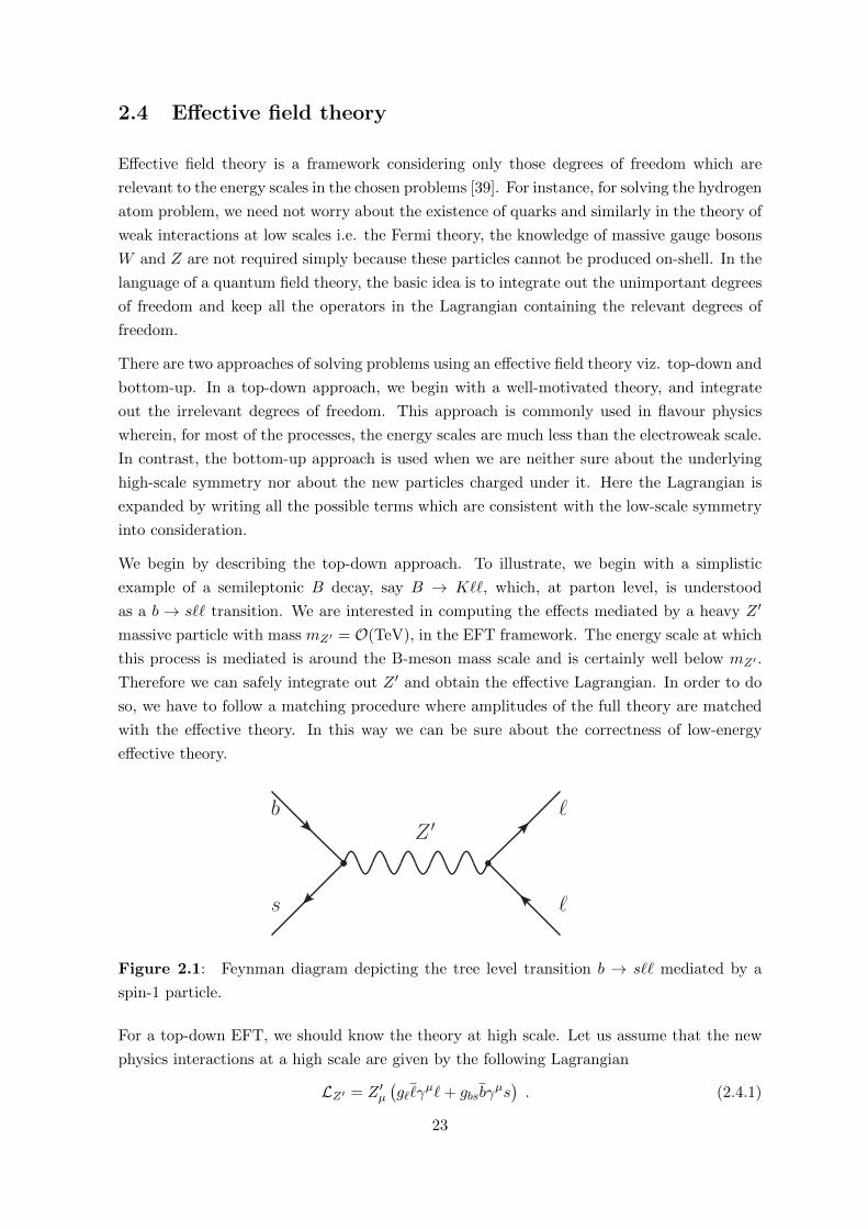
We begin by describing the top-down approach. To illustrate, we begin with a simplistic
example of a semileptonic B decay, say B → K``, which, at parton level, is understood
as a b → s`` transition. We are interested in computing the effects mediated by a heavy Z ′
massive particle with mass mZ′ = O(TeV), in the EFT framework. The energy scale at which
this process is mediated is around the B-meson mass scale and is certainly well below mZ′ .
Therefore we can safely integrate out Z ′ and obtain the effective Lagrangian. In order to do
so, we have to follow a matching procedure where amplitudes of the full theory are matched
with the effective theory. In this way we can be sure about the correctness of low-energy
effective theory.
b
s
ℓ
ℓ
Z ′
Figure 2.1: Feynman diagram depicting the tree level transition b → s`` mediated by a
spin-1 particle.
For a top-down EFT, we should know the theory at high scale. Let us assume that the new
physics interactions at a high scale are given by the following Lagrangian
LZ′ = Z ′µ(g``γ
µ`+ gbsbγµs). (2.4.1)
23
To obtain the effective Lagrangian corresponding to LZ′ , we compute the amplitude in the
full theory following +i convention for obtaining Feynman rules.
iM =
(ig` × igbs ×
−igµνq2 −M2
Z′
)`γµ` bγνs
=
ig` × igbs × i
M2Z′
(1− q2
M2Z′
) `γµ` bγµs (2.4.2)
In the limit q2 � m2Z′
iM = −i (g` × gbs)(
1
M2Z′
+q2
M4Z′
+ . . .
)`γµ` bγµs (2.4.3)
The first term in the series corresponds to the dimension-6 operator, the second one to
dimension-8 and ellipses to further higher dimensional operators. Since q2 �M2Z′ , we safely
concentrate only on the dimension-6 piece which is independent of q2. Now to arrive at
the effective Lagrangian, we make use of the fact that the amplitude of full theory and the
effective field theory are exactly the same. Sticking with the +i convention, we arrive at the
following effective Lagrangian
Leff = −(g` × gbsM2Z′
)`γµ` bγµs . (2.4.4)
The coupling constant of the dimension-6 operator is known as the Wilson coefficient C. Here
C = −g` × gbsM2Z′
. Hence we have illustrated an example of tree-level matching and obtained
the effective Lagrangian and corresponding Wilson coefficient. Since this is obtained at tree-
level, this coefficient does not have any scale dependence and is valid at all scales. Matching
at loop-level introduces a parametric scale dependence on C and also often introduces new
operators.
In contrast, EFTs built using bottom-up principles are arbitrary as the underlying full theory
and the corresponding symmetries are not known. The higher-dimensional terms in the
Lagrangian are written based on the symmetries and particle content of the low energy theory.
The Lagrangian in terms of higher-dimensional operators can then be written as:
Ltot = LSM +∑i
CiΛ2O(dim=6)i +
∑i
CiΛ4O(dim=8)i + . . . , (2.4.5)
where Λ is the scale at which NP enters. If the new physics enters only at the Planck
scale i.e. Λ = 1019 GeV, then the higher dimensional operators are heavily suppressed and
have no effect whatsoever at the current running TeV scaled colliders. However if some new
physics is present at scales much lower than the Planck scales, e.g. near the TeV scale, as
motivated by the hierarchy problem, then the EFT analyses could be useful in pinpointing
the correct vertex structure and eventually the full theory. This analysis although it looks
arbitrary at its face value but is useful since it is not biased by any kind of underlying
24
theory/symmetry. We exemplify this point with a recent example in the literature concerning
the semileptonic B neutral decays. Few years back, an anomaly in the angular observable
of B → K∗µµ differential distribution was reported. During similar times, another anomaly
in the observable RK dealing with B → K transitions was also reported. Although none of
the above anomalies have been seen at the 5σ-level, what is intriguing is the fact that the
bottom-up EFT analysis point towards the dominant presence of new physics in the following
dimension-six operator
O9 =αe4π
[sγµPLb] [µγµµ] (2.4.6)
with the Wilson coefficient Cµ9 = −1. Of course with this single operator there are still many
UV-complete explanations possible but the hope is that if the anomalies are indeed genuine
then the measurements in future will guide us towards a unified theory. Another place where
bottom-up EFT is useful is in parametrising the anomalous contributions to the SM couplings.
The electroweak sector of the SM has been well measured and the constraints on the allowed
values of the corresponding anomalous couplings are quite stringent. The Higgs couplings
in contrast have not been fully measured and still encompass large uncertainties as already
seen in Table. 1.2. The analysis dealing with the anomalous triple gauge coupling using the
bottom-up EFT technique has been performed in chapter 4.
To summarise, one can construct minimal extensions of the Standard Model which help to
study real and projected deviations in the data in a focussed way. This is an easier and more
practical way that the global study of deeper underlying physics, where no particular process
can be studied without bringing into play a slew of theoretical and phenomenological issues.
This is the approach adopted in the present thesis. We now go on to describe some of the
specific analyses carried out within this broad philosophy.
25
Chapter 3
Neutrino mixing and RK anomaly in class of U(1)X
models
In this chapter, we present our findings on the simultaneous solutions to the anomalies seen
in the recent lepton flavour universality violating observables in neutral B-meson decays
and neutrino mixing data. The work has been done in collaboration with Dr. Sabyasachi
Chakraborty and Prof. Amol Dighe and is published in JHEP 1703 (2017) 117.
3.1 Introduction
The run-I data at LHC not only succeeded in discovering a Higgs Boson but also measured
one of the rarest decay predicted in the SM i.e. Bs → µµ [40] with the statistical significance
of more than 6σ. This sole measurement along with B → Xsγ and other neutral meson-
mixings measurements have been responsible for constraining many well defined models like
supersymmetry at the LHC [41,42], which predicts large flavour violations in certain regions
of the parameter space. Although the scales at which B decays operates occur are extremely
small O(mB), they have important implications in constraining the models of NP [43].
In this chapter, we focus on the recently reported indirect hints of lepton flavour universality
violation by the LHCb collaboration in the b→ s`` flavour observables1. The b→ s transitions
at leading order in the Standard Model proceeds through one loop penguin and box diagrams
due to absence of flavour changing neutral currents. These processes are touted to be sensitive
probes as NP effects here are not loop suppressed with respect to the SM contributions.
Experimentally such b → s transitions could be measured as inclusive or exclusive decays of
the Bd,s mesons for instance: B → K∗γ, B → Xsγ, B → K(∗)``, B → Xs``, Bs,d → µµ and
so on. Theoretical calculation of these observables is challenging because of the presence of
form factor uncertainties and non-factorizable QCD corrections. However it is still possible
to construct few observables which are less vulnerable to the QCD corrections. Two such
1Indirect hints have also been reported in the charged B decays, but they lie outside the scope of this
chapter and work.
26
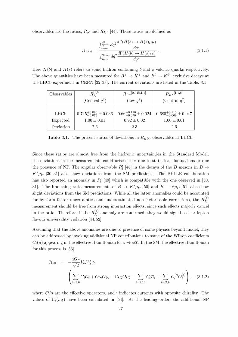
observables are the ratios, RK and RK∗ [44]. These ratios are defined as
RK(∗) =
∫ q2max
q2min
dq2dΓ(H(b)→ H(s)µµ)
dq2∫ q2max
q2min
dq2dΓ(H(b)→ H(s)ee)
dq2
. (3.1.1)
Here H(b) and H(s) refers to some hadron containing b and s valence quarks respectively.
The above quantities have been measured for B+ → K+ and B0 → K0∗ exclusive decays at
the LHCb experiment in CERN [32,33]. The current deviations are listed in the Table. 3.1
Observables R[1,6]K RK∗
[0.045,1.1] RK∗[1.1,6]
(Central q2) (low q2) (Central q2)
LHCb 0.745+0.090−0.074 ± 0.036 0.66+0.110
−0.070 ± 0.024 0.685+0.113−0.069 ± 0.047
Expected 1.00± 0.01 0.92± 0.02 1.00± 0.01
Deviation 2.6 2.3 2.6
Table 3.1: The present status of deviations in RK(∗) observables at LHCb.
Since these ratios are almost free from the hadronic uncertainties in the Standard Model,
the deviations in the measurements could arise either due to statistical fluctuations or due
the presence of NP. The angular observable P ′5 [48] in the decays of the B mesons in B →K∗µµ [30, 31] also show deviations from the SM predictions. The BELLE collaboration
has also reported an anomaly in P ′5 [49] which is compatible with the one observed in [30,
31]. The branching ratio measurements of B → K∗µµ [50] and B → φµµ [51] also show
slight deviations from the SM predictions. While all the latter anomalies could be accounted
for by form factor uncertainties and underestimated non-factorisable corrections, the R(∗)K
measurement should be free from strong interaction effects, since such effects majorly cancel
in the ratio. Therefore, if the R(∗)K anomaly are confirmed, they would signal a clear lepton
flavour universality violation [44,52].
Assuming that the above anomalies are due to presence of some physics beyond model, they
can be addressed by invoking additional NP contributions to some of the Wilson coefficients
Ci(µ) appearing in the effective Hamiltonian for b→ s``. In the SM, the effective Hamiltonian
for this process is [53]
Heff = −4GF√2VtbV
∗ts ×∑
i=1,6
CiOi + C7γO7γ + C8GO8G +∑i=9,10
CiOi +∑i=S,P
C(′)i O
(′)i
, (3.1.2)
where Oi’s are the effective operators, and ′ indicates currents with opposite chirality. The
values of Ci(mb) have been calculated in [54]. At the leading order, the additional NP
27
contributions may contribute to the operators which are already present in the SM:
O7γ =e
16π2mb (sσµνPRb)F
µν , O9 =αe4π
[sγµPLb][¯γµ`
],
O10 =αe4π
[sγµPLb][¯γµγ5`
], (3.1.3)
or may enhance the effects of the operators whose contributions are normally suppressed by
the lepton mass in the SM:
OS =αe4π
[sPRb][¯], OP =
αe4π
[sPRb][¯γ5`
],
O′S =αe4π
[sPLb][¯], O′P =
αe4π
[sPLb][¯γ5`
], (3.1.4)
or may generate new operators which are absent in SM [55]:
O′7γ =e
16π2mb (sσµνPLb)F
µν , O′9 =αe4π
[sγµPRb][¯γµ`
],
O′10 =αe4π
[sγµPRb][¯γµγ5`
]. (3.1.5)
Simultaneous explanation of the RK and P ′5 anomalies2 is possible if the NP effects are present
in O9,O′9,O10 or O′10 operators [56]. The global fits [57–61] prefer NP effects in Oµ9 , i.e.
additional contributions to Cµ9 . Since the observed value of RK(obs) = 0.745+0.090−0.074±0.036 [32]
is less than the SM prediction, which gives RK to be unity within an accuracy of 1% [44,52],
the new physics contribution must interfere destructively with the SM, i.e. opposite to that
of CSM9 (mb) = 4.2 [54]. This indicates that the sign of CNP,µ
9 is negative. The best-fit
value of CNP,µ9 is ≈ −1 [56–61]. In addition CNP,µ
9 = −CNP,µ10 also gives a good fit to data
[58–61]. Motivated by these results, many explanations of the anomaly using Z ′ [62–82] and
leptoquark [56,82–103] models have been given in the literature.
Since the flavour anomalies mentioned above mostly involve muons, and there is no clear hint
of new physics effects in the electron sector apart from RK measurement, most of the analysis
have been performed assuming new physics effects in muons only. However, NP contributions
in the electron sector, CNP,e9 , of the same order as those in the muon sector, are still consistent
with all b → s measurements within 2σ [58–61]. The comparisons among two dimensional
global fits also prefer (CNP,e9 , CNP,µ
9 ) over other combinations like (CNP,µ9 , CNP,µ
10 ) and (CNP,µ9 ,
C ′ NP,µ9 ), with the best fit point favouring dominant contributions to CNP,µ
9 [61].
In this work, we build our analysis around the choice where NP contributes via the O9
operator. We allow both CNP,e9 and CNP,µ
9 to be present. Since these two contributions have
to be different, the NP must violate lepton flavour universality. This may be implemented in a
minimalistic way through an abelian symmetry U(1)X , under which the leptons have different
charges. In particular, greater NP contribution to CNP,µ9 than CNP,e
9 may be achieved by a
higher magnitude of the X-charge for muons than for electrons. Substantial NP contributions
to the flavour anomalies also require tree-level flavour-changing neutral currents (FCNC) in
2The time when the paper was written results of R∗K anomaly were not known, hence the major analysis
in the thesis would concern with RK anomaly. Later in section 3.6, we will comment on the plausibility of
inclusion of RK∗ measurement on the generality of our results.
28
the quark sector. These can be implemented through different X-charges for the quark
generations as well, which should still allow for quark mixing, and be consistent with the
flavour physics data.
A horizontal U(1)X symmetry in the lepton sector would also determine the possible textures
in the mass matrix of the right-handed neutrinos. In turn, the mixing pattern of the left-
handed neutrinos [27,28] will be affected through the Type-I seesaw mechanism. The possible
textures of the right-handed neutrino mass matrix and the lepton flavour universality violation
required for the flavour anomalies can thus have a common origin. Scenarios like an Lµ −Lτsymmetry with X-charges given to the SM quarks [66, 78] or additional vector-like quarks
[65,73], have been considered in the literature in this context. Other models with Z ′ also have
their own X-charge assignments [67,68,70,72,77], however their connection with the neutrino
mass matrix has not been explored. We build our model in the bottom-up approach, where we
do not assign the X-charges a priori, but look for the X-charge assignments that satisfy the
data in the quark and lepton sectors. As a guiding principle, we introduce a minimal number
of additional particles, and ensure that the model is free of any gauge anomalies. Finally,
we identify the horizontal symmetries that are compatible with the observed neutrino mixing
pattern, and at the same time are able to generate CNP,e9 and CNP,µ
9 that explain the flavour
anomalies.
The chapter is organized as follows. In section 3.2, we describe the construction of the U(1)X
models from a bottom-up approach. In section 3.3, we explore the allowed ranges of the
parameters that are consistent with the experimental constraints like neutral meson mixings,
rare B decays, and direct collider searches for Z ′. In section 3.4, we present the predictions for
the CP-violating phases in the lepton sectors for specific horizontal symmetries, and project
the reach of the LHC for detecting the corresponding Z ′. In section 3.5, we summarize our
results and present our concluding remarks.
3.2 Constructing the U(1)X class of models
We construct a class of models wherein, in addition to the SM fields, we also have three right-
handed neutrinos that would be instrumental in giving mass to the left-handed neutrinos
through the seesaw mechanism. We extend the SM gauge symmetry group by an additional
symmetry, U(1)X , which corresponds to an additional gauge boson, Z ′, with mass MZ′ and
gauge coupling gZ′ . To start with, we denote the X-charge for a SM field i by Xi. In this
section, we shall determine the values of Xi’s in a bottom-up approach.
3.2.1 Preliminary constraints on the X-charges
Since we wish to build up the model by introducing NP effects only in theO9 operator, we have
to make sure that the NP contribution to all the other operators listed in eqs. (3.1.3), (3.1.4),
and (3.1.5) should vanish. We first consider the interactions of Z ′ with charged leptons, `, in
29
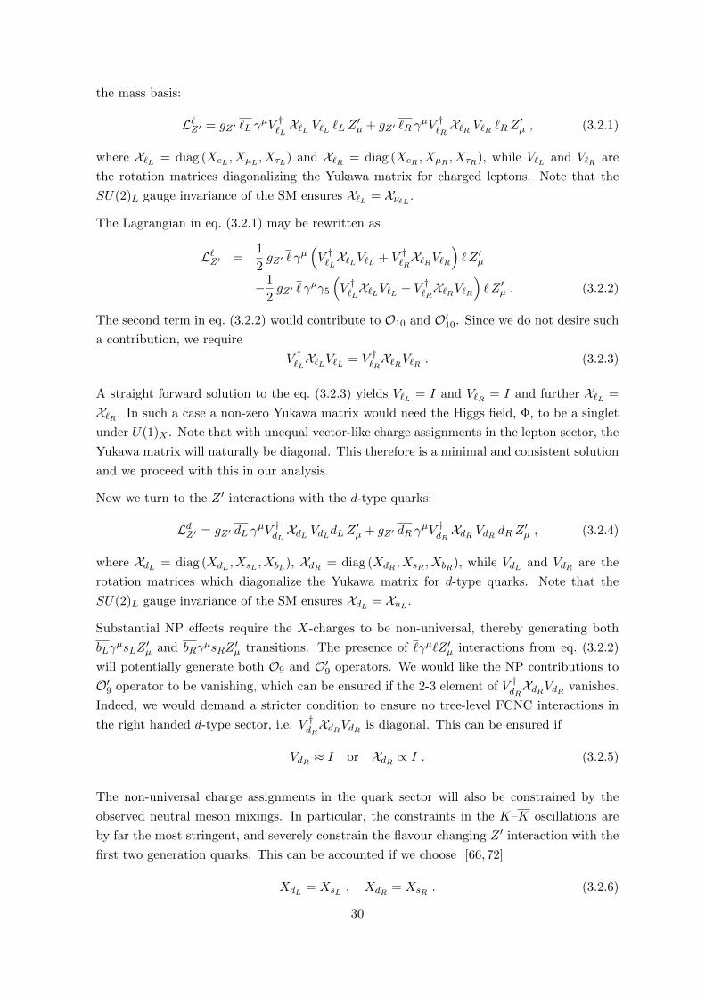
the mass basis:
L`Z′ = gZ′ `L γµV †`L X`L V`L `L Z
′µ + gZ′ `R γ
µV †`R X`R V`R `R Z′µ , (3.2.1)
where X`L = diag (XeL , XµL , XτL) and X`R = diag (XeR , XµR , XτR), while V`L and V`R are
the rotation matrices diagonalizing the Yukawa matrix for charged leptons. Note that the
SU(2)L gauge invariance of the SM ensures X`L = Xν`L .
The Lagrangian in eq. (3.2.1) may be rewritten as
L`Z′ =1
2gZ′ ` γ
µ(V †`LX`LV`L + V †`RX`RV`R
)` Z ′µ
−1
2gZ′ ` γ
µγ5
(V †`LX`LV`L − V
†`RX`RV`R
)` Z ′µ . (3.2.2)
The second term in eq. (3.2.2) would contribute to O10 and O′10. Since we do not desire such
a contribution, we require
V †`LX`LV`L = V †`RX`RV`R . (3.2.3)
A straight forward solution to the eq. (3.2.3) yields V`L = I and V`R = I and further X`L =
X`R . In such a case a non-zero Yukawa matrix would need the Higgs field, Φ, to be a singlet
under U(1)X . Note that with unequal vector-like charge assignments in the lepton sector, the
Yukawa matrix will naturally be diagonal. This therefore is a minimal and consistent solution
and we proceed with this in our analysis.
Now we turn to the Z ′ interactions with the d-type quarks:
LdZ′ = gZ′ dL γµV †dL XdL VdLdL Z
′µ + gZ′ dR γ
µV †dR XdR VdR dR Z′µ , (3.2.4)
where XdL = diag (XdL , XsL , XbL), XdR = diag (XdR , XsR , XbR), while VdL and VdR are the
rotation matrices which diagonalize the Yukawa matrix for d-type quarks. Note that the
SU(2)L gauge invariance of the SM ensures XdL = XuL .
Substantial NP effects require the X-charges to be non-universal, thereby generating both
bLγµsLZ
′µ and bRγ
µsRZ′µ transitions. The presence of `γµ`Z ′µ interactions from eq. (3.2.2)
will potentially generate both O9 and O′9 operators. We would like the NP contributions to
O′9 operator to be vanishing, which can be ensured if the 2-3 element of V †dRXdRVdR vanishes.
Indeed, we would demand a stricter condition to ensure no tree-level FCNC interactions in
the right handed d-type sector, i.e. V †dRXdRVdR is diagonal. This can be ensured if
VdR ≈ I or XdR ∝ I . (3.2.5)
The non-universal charge assignments in the quark sector will also be constrained by the
observed neutral meson mixings. In particular, the constraints in the K–K oscillations are
by far the most stringent, and severely constrain the flavour changing Z ′ interaction with the
first two generation quarks. This can be accounted if we choose [66,72]
XdL = XsL , XdR = XsR . (3.2.6)
30
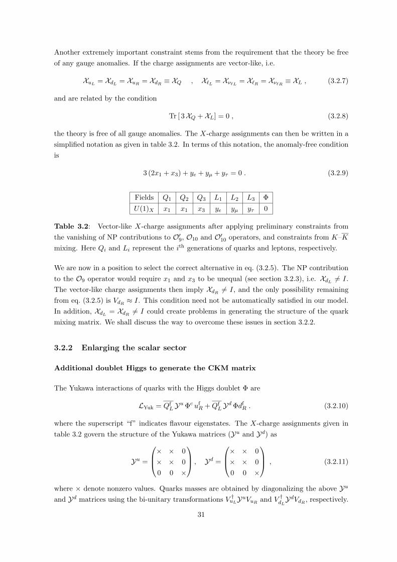
Another extremely important constraint stems from the requirement that the theory be free
of any gauge anomalies. If the charge assignments are vector-like, i.e.
XuL = XdL = XuR = XdR ≡ XQ , X`L = Xν`L = X`R = Xν`R ≡ XL , (3.2.7)
and are related by the condition
Tr [ 3XQ + XL] = 0 , (3.2.8)
the theory is free of all gauge anomalies. The X-charge assignments can then be written in a
simplified notation as given in table 3.2. In terms of this notation, the anomaly-free condition
is
3 (2x1 + x3) + ye + yµ + yτ = 0 . (3.2.9)
Fields Q1 Q2 Q3 L1 L2 L3 Φ
U(1)X x1 x1 x3 ye yµ yτ 0
Table 3.2: Vector-like X-charge assignments after applying preliminary constraints from
the vanishing of NP contributions to O′9, O10 and O′10 operators, and constraints from K–K
mixing. Here Qi and Li represent the ith generations of quarks and leptons, respectively.
We are now in a position to select the correct alternative in eq. (3.2.5). The NP contribution
to the O9 operator would require x1 and x3 to be unequal (see section 3.2.3), i.e. XdL 6= I.
The vector-like charge assignments then imply XdR 6= I, and the only possibility remaining
from eq. (3.2.5) is VdR ≈ I. This condition need not be automatically satisfied in our model.
In addition, XdL = XdR 6= I could create problems in generating the structure of the quark
mixing matrix. We shall discuss the way to overcome these issues in section 3.2.2.
3.2.2 Enlarging the scalar sector
Additional doublet Higgs to generate the CKM matrix
The Yukawa interactions of quarks with the Higgs doublet Φ are
LYuk = QfL Yu Φc uf
R +QfL Yd Φdf
R . (3.2.10)
where the superscript “f” indicates flavour eigenstates. The X-charge assignments given in
table 3.2 govern the structure of the Yukawa matrices (Yu and Yd) as
Yu =
× × 0
× × 0
0 0 ×
, Yd =
× × 0
× × 0
0 0 ×
, (3.2.11)
where × denote nonzero values. Quarks masses are obtained by diagonalizing the above Yuand Yd matrices using the bi-unitary transformations V †uLYuVuR and V †dLY
dVdR , respectively.
31
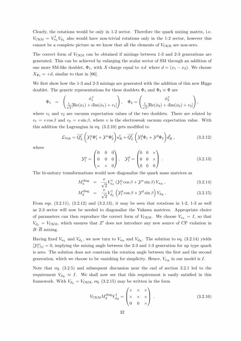
Clearly, the rotations would be only in 1-2 sector. Therefore the quark mixing matrix, i.e.
VCKM = V †uLVdL also would have non-trivial rotations only in the 1-2 sector, however this
cannot be a complete picture as we know that all the elements of VCKM are non-zero.
The correct form of VCKM can be obtained if mixings between 1-3 and 2-3 generations are
generated. This can be achieved by enlarging the scalar sector of SM through an addition of
one more SM-like doublet, Φ1, with X-charge equal to ±d where d = (x1 − x3). We choose
XΦ1 = +d, similar to that in [66].
We first show how the 1-3 and 2-3 mixings are generated with the addition of this new Higgs
doublet. The generic representations for these doublets Φ1 and Φ2 ≡ Φ are
Φ1 =
(φ+
11√2[Re(φ1) + iIm(φ1) + v1]
), Φ2 =
(φ+
21√2[Re(φ2) + iIm(φ2) + v2]
),
where v1 and v2 are vacuum expectation values of the two doublets. There are related by
v1 = v cosβ and v2 = v sinβ, where v is the electroweak vacuum expectation value. With
this addition the Lagrangian in eq. (3.2.10) gets modified to
LYuk = QfL
(Yu1 Φc
1 + YuΦc2
)ufR +Qf
L
(Yd1 Φ1 + YdΦ2
)dfR , (3.2.12)
where
Yu1 =
0 0 0
0 0 0
× × 0
, Yd1 =
0 0 ×0 0 ×0 0 0
. (3.2.13)
The bi-unitary transformations would now diagonalize the quark mass matrices as
Mdiagu =
v√2V †uL (Yu1 cosβ + Yu sinβ)VuR , (3.2.14)
Mdiagd =
v√2V †dL
(Yd1 cosβ + Yd sinβ
)VdR . (3.2.15)
From eqs. (3.2.11), (3.2.12) and (3.2.13), it may be seen that rotations in 1-2, 1-3 as well
as 2-3 sector will now be needed to diagonalize the Yukawa matrices. Appropriate choice
of parameters can then reproduce the correct form of VCKM. We choose VuL = I, so that
VdL = VCKM, which ensures that Z ′ does not introduce any new source of CP violation in
B–B mixing.
Having fixed VuL and VdL , we now turn to VuR and VdR . The solution to eq. (3.2.14) yields
[Yu1 ]ij = 0, implying the mixing angle between the 2-3 and 1-3 generation for up type quark
is zero. The solution does not constrain the rotation angle between the first and the second
generation, which we choose to be vanishing for simplicity. Hence, VuR in our model is I.
Note that eq. (3.2.5) and subsequent discussion near the end of section 3.2.1 led to the
requirement VdR ≈ I. We shall now see that this requirement is easily satisfied in this
framework. With VdL = VCKM, eq. (3.2.15) may be written in the form
VCKMMdiagd V †dR =
× × ×× × ×0 0 ×
. (3.2.16)
32
It may be seen that VdR with small rotation angles, parametrized as
VdR ≈
1 θdR12θdR13
e−i δd
−θdR121 θdR23
−θdR13ei δd −θdR23
1
, (3.2.17)
can lead to the above form, with
θdR23≈ Aλ2ms/mb , θdR13
≈ −Aλ3md/mb , (3.2.18)
where A and λ are the Wolfenstein parameters and md, ms and mb are the quark masses.
Note that similar observation has been made in [66]. The value of θdR12is not constrained,
and can be chosen to be vanishing. Thus, the requirement VdR ≈ 1 is satisfied.
Note that since VdR is only approximately equal to I, small NP contributions to C ′9 are present,
However as we shall see in section 3.2.3, these contributions are roughly (Aλ2ms)/(mbVtbV∗ts)
times the NP contributions to C9, and hence can be safely neglected.
Singlet scalar for generating neutrino masses and mixing pattern
Our model has three right handed neutrinos, νR’s. The Dirac and the Majorana mass terms
for neutrinos are
Lmassν = −νLmDνR −
1
2νcRMRνR + h.c. , (3.2.19)
where the basis chosen for νL is such that the charged lepton mass matrix is diagonal. The
active neutrinos would then get their masses through the Type-I seesaw mechanism. The net
mass matrix being
Mν = −mDM−1R mT
D . (3.2.20)
Since the neutrinos are charged under U(1)X with charges (ye,yµ and yτ ), the (α, β) elements
of the Dirac mass matrix mD would be nonzero only when yα = yβ, while the (α, β) elements
of the Majorana mass matrix MR would be nonzero only when yα + yβ = 0. Since the X-
charges of neutrinos are non-universal and vector-like, the former condition implies that mD
is diagonal. (It can have off-diagonal elements if two of the yα’s are identical. However we can
always choose the νR basis such that mD is diagonal.) The allowed elements of MR are also
severely restricted, and it will not be possible to have a sufficient number of nonzero elements
in MR to be able to generate the neutrino mixing pattern.
To generate the required mixing pattern, we introduce a scalar S, which is a SM-singlet, and
has an X-charge XS = a, as a minimal extension of our model. With the addition of this
scalar, the Lagrangian in eq. (3.2.19) modifies to
[Lmass,Sν ]αβ = [Lmass
ν ]αβ −1
2[νcR]α[YR]αβ[νR]β S + h.c. . (3.2.21)
The conditions for mD, MR and YR elements to be non zero are
[mD]αβ 6= 0 if yα − yβ = 0 , (3.2.22)
[MR]αβ 6= 0 if yα + yβ = 0 ,
[YR]αβ 6= 0 if yα + yβ = ±a . (3.2.23)
33
When S gets a vacuum expectation value vS , it contributes to the Majorana mass term for
right handed neutrinos which now becomes
[MSR]αβ = [MR]αβ +
vS√2
[yR]αβ . (3.2.24)
Thus an element of [MSR]αβ will be non-zero if,
yα + yβ = 0,±a . (3.2.25)
The textures in the neutrino mass matrix, i.e. the number and location of vanishing elements
therein, hold clues to the internal flavour symmetries. Only some specific textures of MR
are allowed. While no three-zero textures are consistent with data, specific two-zero textures
are allowed [104–107]. In addition, most one-zero textures [108], and naturally, all no-zero
textures, are also permitted. Among the allowed textures, we identify those that can be
generated by a U(1)X symmetry with a singlet scalar, i.e. those for which values of yα
and a satisfying eq. (3.2.25) may be found. These combinations are listed in table 3.3, and
categorized according to the ratio ye/yµ. Note that by the leptonic symmetry combination
peLe+pµLµ+pτLτ , we refer to all U(1)X charge combinations, where pe/ye = pµ/yµ = pτ/yτ
(for non zero values yα and pα respectively). It is to be noted that part of the list was
already derived in [106,107]. Later in section 3.2.3, we shall examine the consistency of these
symmetries with the flavour data.
Note that we would like all the elements of right handed neutrino mass matrix to have similar
magnitudes, so it would be natural to have [MSR]α,β ∼ O(vS). Our scenario is thus close to a
TeV-scale seesaw mechanism [109].
Relating X-charges of doublet and singlet scalars
The scalar sector of our model consists of two SU(2)L doublets Φ1 and Φ ≡ Φ2, and a
SM-singlet S, with X-charges d, 0, a, respectively. The scalar potential that respects the
SU(2)L × U(1)Y × U(1)X symmetry is
VΦ1Φ2S = −m211Φ†1Φ1 +
λ1
2(Φ†1Φ1)2 −m2
22Φ†2Φ2 +λ2
2(Φ†2Φ2)2
−m2SS†S +
λS2
(S†S)2 + λ3 Φ†1Φ1 Φ†2Φ2
+λ4 Φ†1Φ2 Φ†2Φ1 +(λ1S1Φ†1Φ1 + λ2SΦ†2Φ2
)S†S . (3.2.26)
The U(1)X symmetry is broken spontaneously by the vacuum expectation values of Φ1 and
S, and consequently Z ′ obtains a mass (see section 2.3). Since the collider bounds indicate
MZ′ & TeV, we expect vs & TeV (since v1 . electroweak scale).
Therefore, before electroweak symmetry breaking, U(1)X symmetry gets broken sponta-
neously and the singlet, S, gets decoupled. The effective potential for the doublets after
34
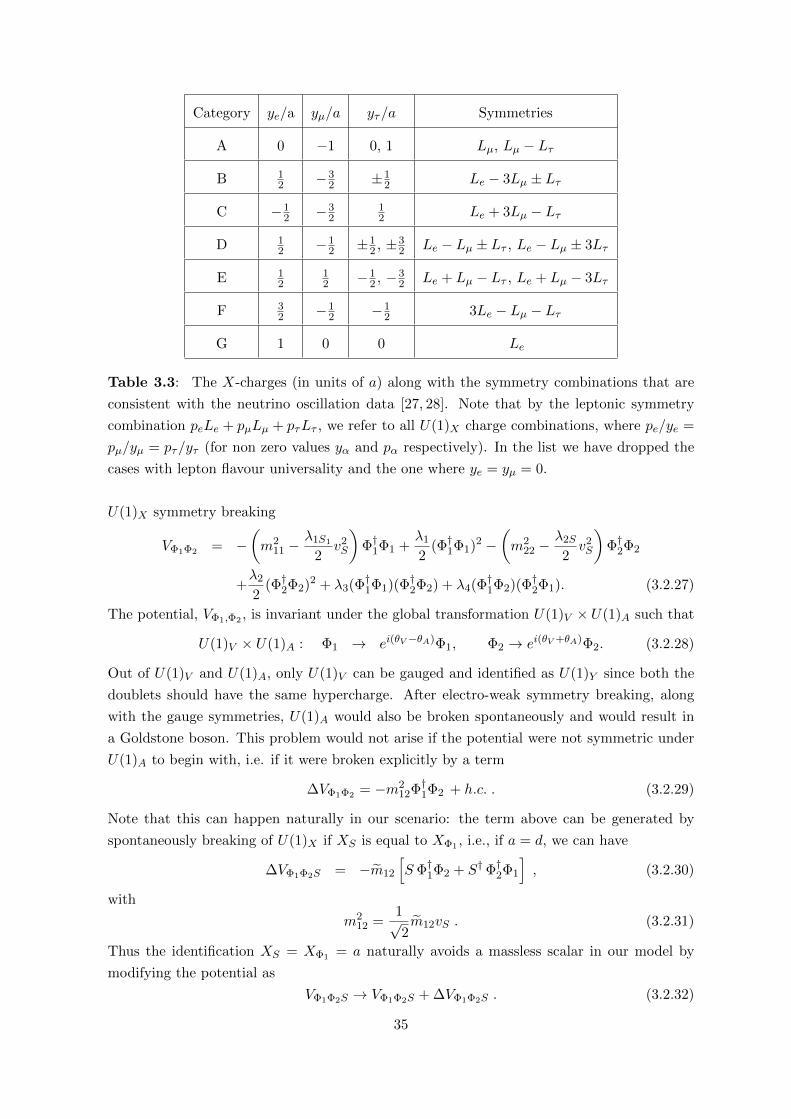
Category ye/a yµ/a yτ/a Symmetries
A 0 −1 0, 1 Lµ, Lµ − Lτ
B 12 −3
2 ±12 Le − 3Lµ ± Lτ
C −12 −3
212 Le + 3Lµ − Lτ
D 12 −1
2 ±12 , ±3
2 Le − Lµ ± Lτ , Le − Lµ ± 3Lτ
E 12
12 −1
2 , −32 Le + Lµ − Lτ , Le + Lµ − 3Lτ
F 32 −1
2 −12 3Le − Lµ − Lτ
G 1 0 0 Le
Table 3.3: The X-charges (in units of a) along with the symmetry combinations that are
consistent with the neutrino oscillation data [27, 28]. Note that by the leptonic symmetry
combination peLe + pµLµ + pτLτ , we refer to all U(1)X charge combinations, where pe/ye =
pµ/yµ = pτ/yτ (for non zero values yα and pα respectively). In the list we have dropped the
cases with lepton flavour universality and the one where ye = yµ = 0.
U(1)X symmetry breaking
VΦ1Φ2 = −(m2
11 −λ1S1
2v2S
)Φ†1Φ1 +
λ1
2(Φ†1Φ1)2 −
(m2
22 −λ2S
2v2S
)Φ†2Φ2
+λ2
2(Φ†2Φ2)2 + λ3(Φ†1Φ1)(Φ†2Φ2) + λ4(Φ†1Φ2)(Φ†2Φ1). (3.2.27)
The potential, VΦ1,Φ2 , is invariant under the global transformation U(1)V × U(1)A such that
U(1)V × U(1)A : Φ1 → ei(θV −θA)Φ1, Φ2 → ei(θV +θA)Φ2. (3.2.28)
Out of U(1)V and U(1)A, only U(1)V can be gauged and identified as U(1)Y since both the
doublets should have the same hypercharge. After electro-weak symmetry breaking, along
with the gauge symmetries, U(1)A would also be broken spontaneously and would result in
a Goldstone boson. This problem would not arise if the potential were not symmetric under
U(1)A to begin with, i.e. if it were broken explicitly by a term
∆VΦ1Φ2 = −m212Φ†1Φ2 + h.c. . (3.2.29)
Note that this can happen naturally in our scenario: the term above can be generated by
spontaneously breaking of U(1)X if XS is equal to XΦ1 , i.e., if a = d, we can have
∆VΦ1Φ2S = −m12
[S Φ†1Φ2 + S†Φ†2Φ1
], (3.2.30)
with
m212 =
1√2m12vS . (3.2.31)
Thus the identification XS = XΦ1 = a naturally avoids a massless scalar in our model by
modifying the potential as
VΦ1Φ2S → VΦ1Φ2S + ∆VΦ1Φ2S . (3.2.32)
35
3.2.3 Selection of the desirable symmetry combinations
In this section, we combine the U(1)X symmetries identified in section 3.2.2 with the NP
contribution to O9 needed to account for the flavour anomalies. The Lagrangian describing
the Z ′ interactions with d-type quarks and charged leptons is
LZ′ = gZ′ dLγµ V †CKMXQ VCKMdL Z
′µ + gZ′ dR γ
µ V †dR XQ VdR dR Z′µ
+gZ′ ` γµXL ` Z ′µ (3.2.33)
Here XQ = diag(x1, x1, x3) and XL = diag(ye, yµ, yτ ). Using the above Lagrangian, the Z ′
contributions to the effective Hamiltonian for b→ s`` processes at MZ′ scale is
HNPeff = −(x1 − x3) y` g
2Z′
M2Z′
VtbV∗ts (sLγ
µbL)(`γµ`
)+
(x1 − x3) y` g2Z′
M2Z′
θ2dR23
(sRγµbR)
(`γµ`
).
(3.2.34)
Comparing it with the standard definition of Heff as given in eq. (3.1.2), we obtain the NP
contribution to the Wilson coefficients CNP,`9 and C ′NP,`
9 as
CNP,`9 (MZ
′) =
√2π(x1 − x3) y`g
2Z′
GFM2Z′αe
, C ′NP,`9 (MZ
′) = −√
2π(x1 − x3) y`g2Z′θ
2dR23
GFM2Z′αeVtbV
∗ts
, (3.2.35)
The smallness of θR23, as shown in eq (3.2.18), makes the NP contribution to O′9 small in
comparison to the corresponding contribution to O9:
C ′`9 (MZ′) = −
θ2DR23
VtbV∗ts
CNP,`9 (MZ
′)
≈ −0.025CNP,`9 (MZ
′) . (3.2.36)
The flavour anomalies like RK and P ′5 depend crucially on CNP,e9 and CNP,µ
9 , and not on
CNP,τ9 . A negative value of CNP,µ
9 is preferred [57–61] as a solution to these anomalies which
can be easily obtained if, (x1 − x3) yµ < 0. The values of CNP,e9 and CNP,µ
9 are related by
CNP,e9 /CNP,µ
9 = ye/yµ . (3.2.37)
This ratio stays the same at all scales between MZ′ and mb, since the O9 operator does not
mix with any other operator at one loop in QCD. This ratio is represented in figure 3.1 by
lines corresponding to different symmetries in table 3.3.
In figure 3.1, we also show the 1σ contours in the CNP,µ9 –CNP,e
9 plane obtained from the
global fits [59–61]. For further analysis, we select only those combinations (categories A, B,
C, D) which pass through the 1σ regions of any of these global fit contours. Among these
possibilities, Lµ − Lτ has already been considered in the context of RK [65,66,73,78], where
the NP contribution to Ce9 is absent. We shall explore the phenomenological consequences of
these symmetries in section 3.3.
Note that although we refer to the symmetries by their lepton combinations, quarks are also
charged under the U(1)X . These charges can be easily obtained from the anomaly eq. (3.2.9),
36
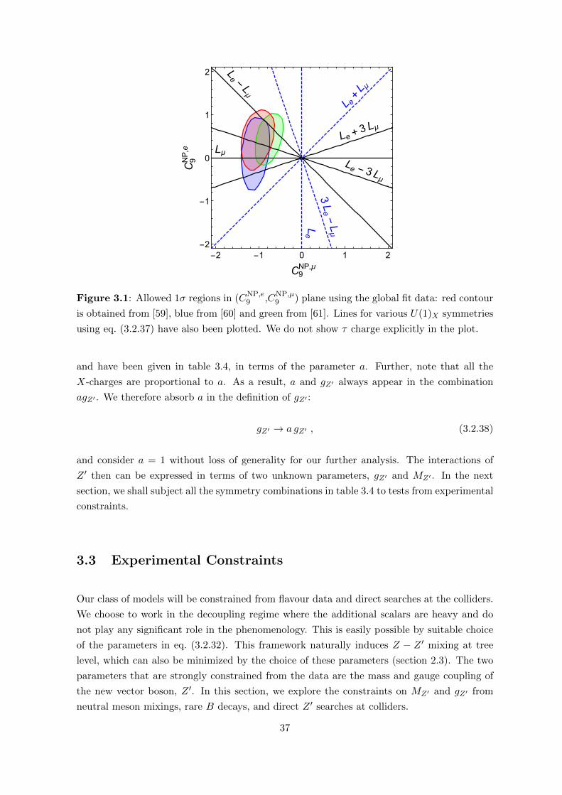
Le -Lμ
Le - 3 Lμ
Lμ
Le+ 3Lμ
L e+L μ
Le
3Le-Lμ
-2 -1 0 1 2
-2
-1
0
1
2
C9NP,μ
C9NP,e
Figure 3.1: Allowed 1σ regions in (CNP,e9 ,CNP,µ
9 ) plane using the global fit data: red contour
is obtained from [59], blue from [60] and green from [61]. Lines for various U(1)X symmetries
using eq. (3.2.37) have also been plotted. We do not show τ charge explicitly in the plot.
and have been given in table 3.4, in terms of the parameter a. Further, note that all the
X-charges are proportional to a. As a result, a and gZ′ always appear in the combination
agZ′ . We therefore absorb a in the definition of gZ′ :
gZ′ → a gZ′ , (3.2.38)
and consider a = 1 without loss of generality for our further analysis. The interactions of
Z ′ then can be expressed in terms of two unknown parameters, gZ′ and MZ′ . In the next
section, we shall subject all the symmetry combinations in table 3.4 to tests from experimental
constraints.
3.3 Experimental Constraints
Our class of models will be constrained from flavour data and direct searches at the colliders.
We choose to work in the decoupling regime where the additional scalars are heavy and do
not play any significant role in the phenomenology. This is easily possible by suitable choice
of the parameters in eq. (3.2.32). This framework naturally induces Z − Z ′ mixing at tree
level, which can also be minimized by the choice of these parameters (section 2.3). The two
parameters that are strongly constrained from the data are the mass and gauge coupling of
the new vector boson, Z ′. In this section, we explore the constraints on MZ′ and gZ′ from
neutral meson mixings, rare B decays, and direct Z ′ searches at colliders.
37
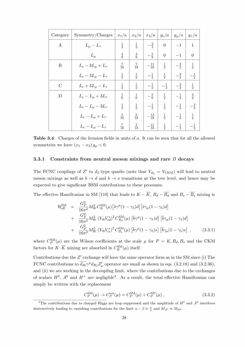
Category Symmetry/Charges x1/a x2/a x3/a ye/a yµ/a yτ/a
A Lµ − Lτ 13
13 −2
3 0 −1 1
Lµ49
49 −5
9 0 −1 0
B Le − 3Lµ + Lτ718
718 −11
1812 −3
212
Le − 3Lµ − Lτ 12
12 −1
212 −3
2 −12
C Le + 3Lµ − Lτ 12
12 −1
2 −12 −3
212
D Le − Lµ + 3Lτ16
16 −5
612 −1
232
Le − Lµ − 3Lτ12
12 −1
212 −1
2 −32
Le − Lµ + Lτ518
518 −13
1812 −1
212
Le − Lµ − Lτ 718
718 −11
1812 −1
2 −12
Table 3.4: Charges of the fermion fields in units of a. It can be seen that for all the allowed
symmetries we have (x1 − x3) yµ < 0.
3.3.1 Constraints from neutral meson mixings and rare B decays
The FCNC couplings of Z ′ to dL-type quarks (note that VdL = VCKM) will lead to neutral
meson mixings as well as b → d and b → s transitions at the tree level, and hence may be
expected to give significant BSM contributions to these processes.
The effective Hamiltonian in SM [110] that leads to K −K, Bd −Bd and Bs −Bs mixing is
HSMeff =
G2F
16π2M2WC
SMK (µ)
[sγµ(1− γ5)d
][sγµ(1− γ5)d
]+
G2F
16π2M2W (VtbV
∗td)
2CSMBd
(µ)[bγµ(1− γ5)d
] [bγµ(1− γ5)d
]+
G2F
16π2M2W (VtbV
∗ts)
2CSMBs (µ)
[bγµ(1− γ5)s
] [bγµ(1− γ5)s
], (3.3.1)
where CSMP (µ) are the Wilson coefficients at the scale µ for P = K,Bd, Bs and the CKM
factors for K–K mixing are absorbed in CSMK (µ) itself.
Contributions due the Z ′ exchange will have the same operator form as in the SM since (i) The
FCNC contributions to dRiγµdRjZ
′µ operator are small as shown in eqs. (3.2.18) and (3.2.36),
and (ii) we are working in the decoupling limit, where the contributions due to the exchanges
of scalars H0, A0 and H+ are negligible3. As a result, the total effective Hamiltonian can
simply be written with the replacement
CSMP (µ)→ Ctot
P (µ) = CSMP (µ) + CNP
P (µ) , (3.3.2)
3The contributions due to charged Higgs are loop suppressed and the amplitude of H0 and A0 interferes
destructively leading to vanishing contributions for the limit α− β ≈ π2
and MA0 ≈MH0 .
38
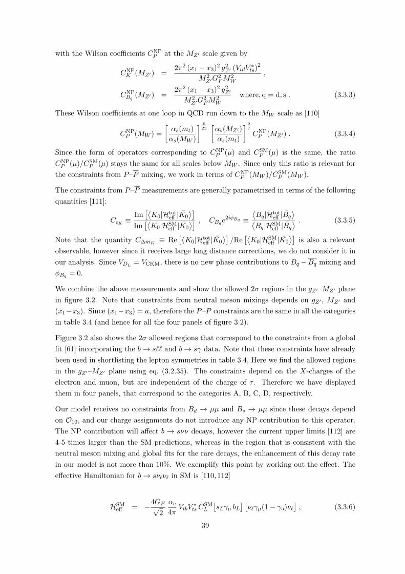
with the Wilson coefficients CNPP at the MZ′ scale given by
CNPK (MZ′) =
2π2 (x1 − x3)2 g2Z′ (VtdV
∗ts)
2
M2Z′G
2FM
2W
,
CNPBq (MZ′) =
2π2 (x1 − x3)2 g2Z′
M2Z′G
2FM
2W
where, q = d, s . (3.3.3)
These Wilson coefficients at one loop in QCD run down to the MW scale as [110]
CNPP (MW ) =
[αs(mt)
αs(MW )
] 623[αs(MZ′)
αs(mt)
] 27
CNPP (MZ′) . (3.3.4)
Since the form of operators corresponding to CNPP (µ) and CSM
P (µ) is the same, the ratio
CNPP (µ)/CSM
P (µ) stays the same for all scales below MW . Since only this ratio is relevant for
the constraints from P–P mixing, we work in terms of CNPP (MW )/CSM
P (MW ).
The constraints from P–P measurements are generally parametrized in terms of the following
quantities [111]:
CεK ≡Im[⟨K0|Htot
eff |K0
⟩]Im[⟨K0|HSM
eff |K0
⟩] , CBqe2iφBq ≡
⟨Bq|Htot
eff |Bq⟩⟨
Bq|HSMeff |Bq
⟩ . (3.3.5)
Note that the quantity C∆mK ≡ Re[⟨K0|Htot
eff |K0
⟩]/Re
[⟨K0|HSM
eff |K0
⟩]is also a relevant
observable, however since it receives large long distance corrections, we do not consider it in
our analysis. Since VDL = VCKM, there is no new phase contributions to Bq −Bq mixing and
φBq = 0.
We combine the above measurements and show the allowed 2σ regions in the gZ′–MZ′ plane
in figure 3.2. Note that constraints from neutral meson mixings depends on gZ′ , MZ′ and
(x1−x3). Since (x1−x3) = a, therefore the P–P constraints are the same in all the categories
in table 3.4 (and hence for all the four panels of figure 3.2).
Figure 3.2 also shows the 2σ allowed regions that correspond to the constraints from a global
fit [61] incorporating the b→ s`` and b→ sγ data. Note that these constraints have already
been used in shortlisting the lepton symmetries in table 3.4, Here we find the allowed regions
in the gZ′–MZ′ plane using eq. (3.2.35). The constraints depend on the X-charges of the
electron and muon, but are independent of the charge of τ . Therefore we have displayed
them in four panels, that correspond to the categories A, B, C, D, respectively.
Our model receives no constraints from Bd → µµ and Bs → µµ since these decays depend
on O10, and our charge assignments do not introduce any NP contribution to this operator.
The NP contribution will affect b → sνν decays, however the current upper limits [112] are
4-5 times larger than the SM predictions, whereas in the region that is consistent with the
neutral meson mixing and global fits for the rare decays, the enhancement of this decay rate
in our model is not more than 10%. We exemplify this point by working out the effect. The
effective Hamiltonian for b→ sν`ν` in SM is [110,112]
HSMeff = −4GF√
2
αe4π
VtbV∗tsC
SML
[sLγµ bL
] [ν`γµ(1− γ5)ν`
], (3.3.6)
39
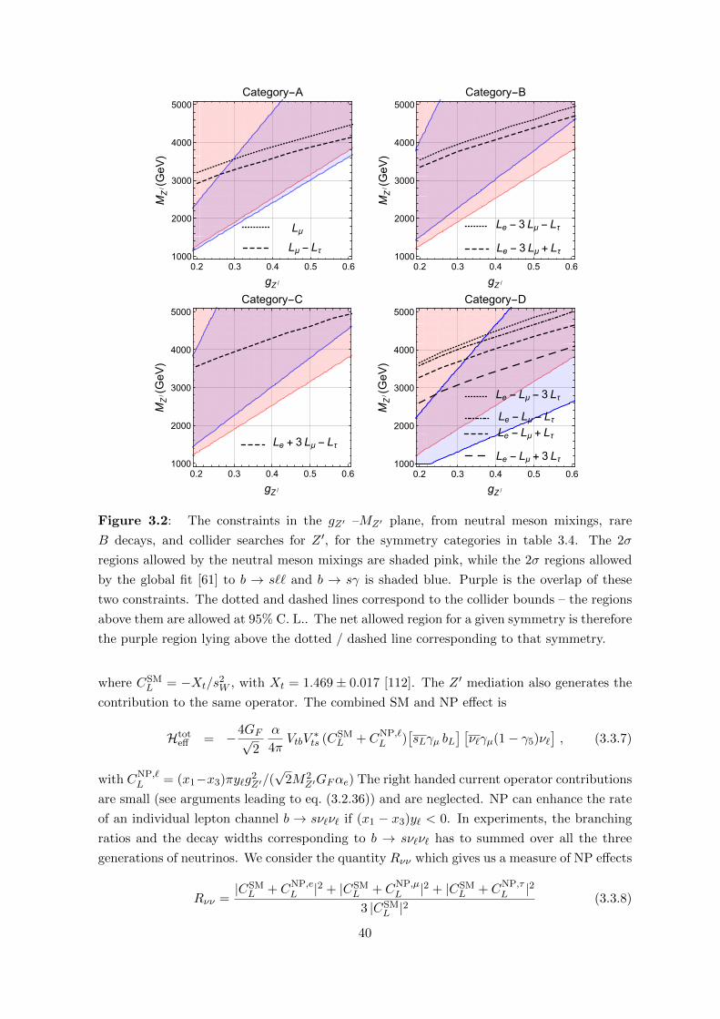
Lμ
Lμ - Lτ
0.2 0.3 0.4 0.5 0.61000
2000
3000
4000
5000
gZ /
MZ
/(GeV)
Category-A
Le - 3 Lμ + Lτ
Le - 3 Lμ - Lτ
0.2 0.3 0.4 0.5 0.61000
2000
3000
4000
5000
gZ /
MZ
/(GeV)
Category-B
Le + 3 Lμ - Lτ
0.2 0.3 0.4 0.5 0.61000
2000
3000
4000
5000
gZ /
MZ
/(GeV)
Category-C
Le - Lμ + 3 Lτ
Le - Lμ - 3 Lτ
Le - Lμ - LτLe - Lμ + Lτ
0.2 0.3 0.4 0.5 0.61000
2000
3000
4000
5000
gZ /
MZ
/(GeV)
Category-D
Figure 3.2: The constraints in the gZ′ –MZ′ plane, from neutral meson mixings, rare
B decays, and collider searches for Z ′, for the symmetry categories in table 3.4. The 2σ
regions allowed by the neutral meson mixings are shaded pink, while the 2σ regions allowed
by the global fit [61] to b → s`` and b → sγ is shaded blue. Purple is the overlap of these
two constraints. The dotted and dashed lines correspond to the collider bounds – the regions
above them are allowed at 95% C. L.. The net allowed region for a given symmetry is therefore
the purple region lying above the dotted / dashed line corresponding to that symmetry.
where CSML = −Xt/s
2W , with Xt = 1.469± 0.017 [112]. The Z ′ mediation also generates the
contribution to the same operator. The combined SM and NP effect is
Htoteff = −4GF√
2
α
4πVtbV
∗ts (CSM
L + CNP,`L )
[sLγµ bL
] [ν`γµ(1− γ5)ν`
], (3.3.7)
with CNP,`L = (x1−x3)πy`g
2Z′/(√
2M2Z′GFαe) The right handed current operator contributions
are small (see arguments leading to eq. (3.2.36)) and are neglected. NP can enhance the rate
of an individual lepton channel b → sν`ν` if (x1 − x3)y` < 0. In experiments, the branching
ratios and the decay widths corresponding to b → sν`ν` has to summed over all the three
generations of neutrinos. We consider the quantity Rνν which gives us a measure of NP effects
Rνν =|CSML + CNP,e
L |2 + |CSML + CNP,µ
L |2 + |CSML + CNP,τ
L |23 |CSM
L |2(3.3.8)
40
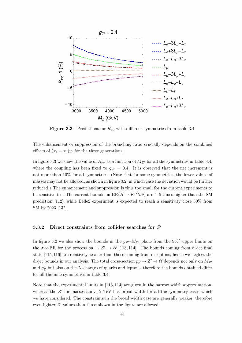
3000 3500 4000 4500 5000
-10
-5
0
5
10
MZ /(GeV)
Rνν-1(%
)
gZ / = 0.4
Le-3Lμ-Lτ
Le+3Lμ-Lτ
Le-Lμ-3Lτ
Lμ
Le-3Lμ+Lτ
Le-Lμ-Lτ
Lμ-Lτ
Le-Lμ+Lτ
Le-Lμ+3Lτ
Figure 3.3: Predictions for Rνν with different symmetries from table 3.4.
The enhancement or suppression of the branching ratio crucially depends on the combined
effects of (x1 − x3)y` for the three generations.
In figure 3.3 we show the value of Rνν as a function of MZ′ for all the symmetries in table 3.4,
where the coupling has been fixed to gZ′ = 0.4. It is observed that the net increment is
not more than 10% for all symmetries. (Note that for some symmetries, the lower values of
masses may not be allowed, as shown in figure 3.2, in which case the deviation would be further
reduced.) The enhancement and suppression is thus too small for the current experiments to
be sensitive to – The current bounds on BR(B → K(∗)νν) are 4–5 times higher than the SM
prediction [112], while Belle2 experiment is expected to reach a sensitivity close 30% from
SM by 2023 [132].
3.3.2 Direct constraints from collider searches for Z ′
In figure 3.2 we also show the bounds in the gZ′–MZ′ plane from the 95% upper limits on
the σ × BR for the process pp → Z ′ → `` [113, 114]. The bounds coming from di-jet final
state [115,116] are relatively weaker than those coming from di-leptons, hence we neglect the
di-jet bounds in our analysis. The total cross-section pp→ Z ′ → `` depends not only on MZ′
and g′Z but also on the X-charges of quarks and leptons, therefore the bounds obtained differ
for all the nine symmetries in table 3.4.
Note that the experimental limits in [113,114] are given in the narrow width approximation,
whereas the Z ′ for masses above 2 TeV has broad width for all the symmetry cases which
we have considered. The constraints in the broad width case are generally weaker, therefore
even lighter Z ′ values than those shown in the figure are allowed.
41
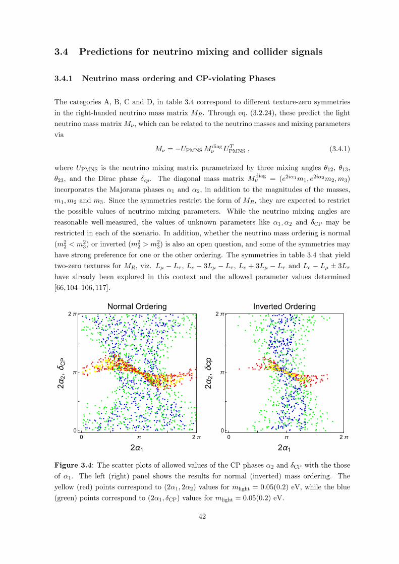
3.4 Predictions for neutrino mixing and collider signals
3.4.1 Neutrino mass ordering and CP-violating Phases
The categories A, B, C and D, in table 3.4 correspond to different texture-zero symmetries
in the right-handed neutrino mass matrix MR. Through eq. (3.2.24), these predict the light
neutrino mass matrix Mν , which can be related to the neutrino masses and mixing parameters
via
Mν = −UPMNSMdiagν UTPMNS , (3.4.1)
where UPMNS is the neutrino mixing matrix parametrized by three mixing angles θ12, θ13,
θ23, and the Dirac phase δcp. The diagonal mass matrix Mdiagν = (e2iα1m1, e
2iα2m2,m3)
incorporates the Majorana phases α1 and α2, in addition to the magnitudes of the masses,
m1,m2 and m3. Since the symmetries restrict the form of MR, they are expected to restrict
the possible values of neutrino mixing parameters. While the neutrino mixing angles are
reasonable well-measured, the values of unknown parameters like α1, α2 and δCP may be
restricted in each of the scenario. In addition, whether the neutrino mass ordering is normal
(m22 < m2
3) or inverted (m22 > m2
3) is also an open question, and some of the symmetries may
have strong preference for one or the other ordering. The symmetries in table 3.4 that yield
two-zero textures for MR, viz. Lµ − Lτ , Le − 3Lµ − Lτ , Le + 3Lµ − Lτ and Le − Lµ ± 3Lτ
have already been explored in this context and the allowed parameter values determined
[66,104–106,117].
0 π 2 π0
π
2 π
2α1
2α2,δCP
Normal Ordering
0 π 2 π0
π
2 π
2α1
2α2,δcp
Inverted Ordering
Figure 3.4: The scatter plots of allowed values of the CP phases α2 and δCP with the those
of α1. The left (right) panel shows the results for normal (inverted) mass ordering. The
yellow (red) points correspond to (2α1, 2α2) values for mlight = 0.05(0.2) eV, while the blue
(green) points correspond to (2α1, δCP) values for mlight = 0.05(0.2) eV.
42
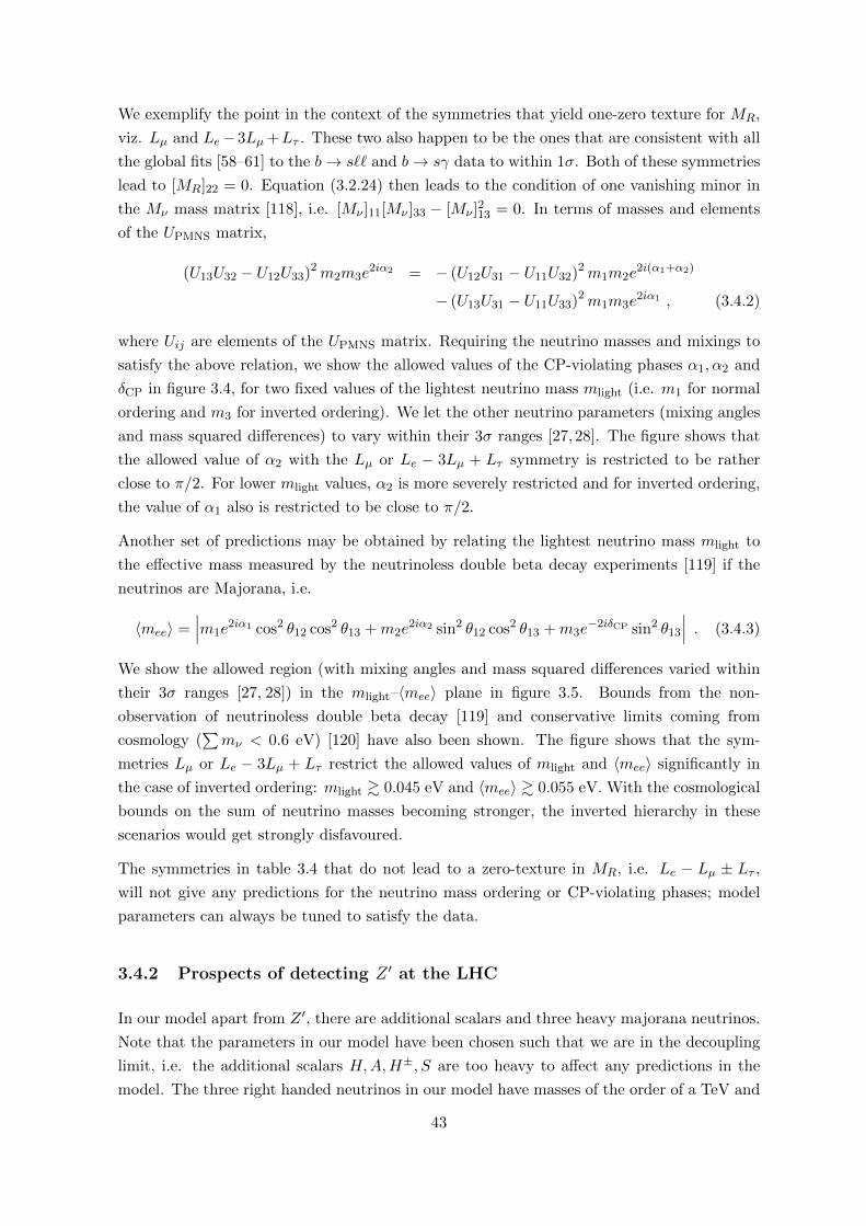
We exemplify the point in the context of the symmetries that yield one-zero texture for MR,
viz. Lµ and Le− 3Lµ +Lτ . These two also happen to be the ones that are consistent with all
the global fits [58–61] to the b→ s`` and b→ sγ data to within 1σ. Both of these symmetries
lead to [MR]22 = 0. Equation (3.2.24) then leads to the condition of one vanishing minor in
the Mν mass matrix [118], i.e. [Mν ]11[Mν ]33 − [Mν ]213 = 0. In terms of masses and elements
of the UPMNS matrix,
(U13U32 − U12U33)2m2m3e2iα2 = − (U12U31 − U11U32)2m1m2e
2i(α1+α2)
− (U13U31 − U11U33)2m1m3e2iα1 , (3.4.2)
where Uij are elements of the UPMNS matrix. Requiring the neutrino masses and mixings to
satisfy the above relation, we show the allowed values of the CP-violating phases α1, α2 and
δCP in figure 3.4, for two fixed values of the lightest neutrino mass mlight (i.e. m1 for normal
ordering and m3 for inverted ordering). We let the other neutrino parameters (mixing angles
and mass squared differences) to vary within their 3σ ranges [27, 28]. The figure shows that
the allowed value of α2 with the Lµ or Le − 3Lµ + Lτ symmetry is restricted to be rather
close to π/2. For lower mlight values, α2 is more severely restricted and for inverted ordering,
the value of α1 also is restricted to be close to π/2.
Another set of predictions may be obtained by relating the lightest neutrino mass mlight to
the effective mass measured by the neutrinoless double beta decay experiments [119] if the
neutrinos are Majorana, i.e.
〈mee〉 =∣∣∣m1e
2iα1 cos2 θ12 cos2 θ13 +m2e2iα2 sin2 θ12 cos2 θ13 +m3e
−2iδCP sin2 θ13
∣∣∣ . (3.4.3)
We show the allowed region (with mixing angles and mass squared differences varied within
their 3σ ranges [27, 28]) in the mlight–〈mee〉 plane in figure 3.5. Bounds from the non-
observation of neutrinoless double beta decay [119] and conservative limits coming from
cosmology (∑mν < 0.6 eV) [120] have also been shown. The figure shows that the sym-
metries Lµ or Le − 3Lµ + Lτ restrict the allowed values of mlight and 〈mee〉 significantly in
the case of inverted ordering: mlight & 0.045 eV and 〈mee〉 & 0.055 eV. With the cosmological
bounds on the sum of neutrino masses becoming stronger, the inverted hierarchy in these
scenarios would get strongly disfavoured.
The symmetries in table 3.4 that do not lead to a zero-texture in MR, i.e. Le − Lµ ± Lτ ,
will not give any predictions for the neutrino mass ordering or CP-violating phases; model
parameters can always be tuned to satisfy the data.
3.4.2 Prospects of detecting Z ′ at the LHC
In our model apart from Z ′, there are additional scalars and three heavy majorana neutrinos.
Note that the parameters in our model have been chosen such that we are in the decoupling
limit, i.e. the additional scalars H,A,H±, S are too heavy to affect any predictions in the
model. The three right handed neutrinos in our model have masses of the order of a TeV and
43
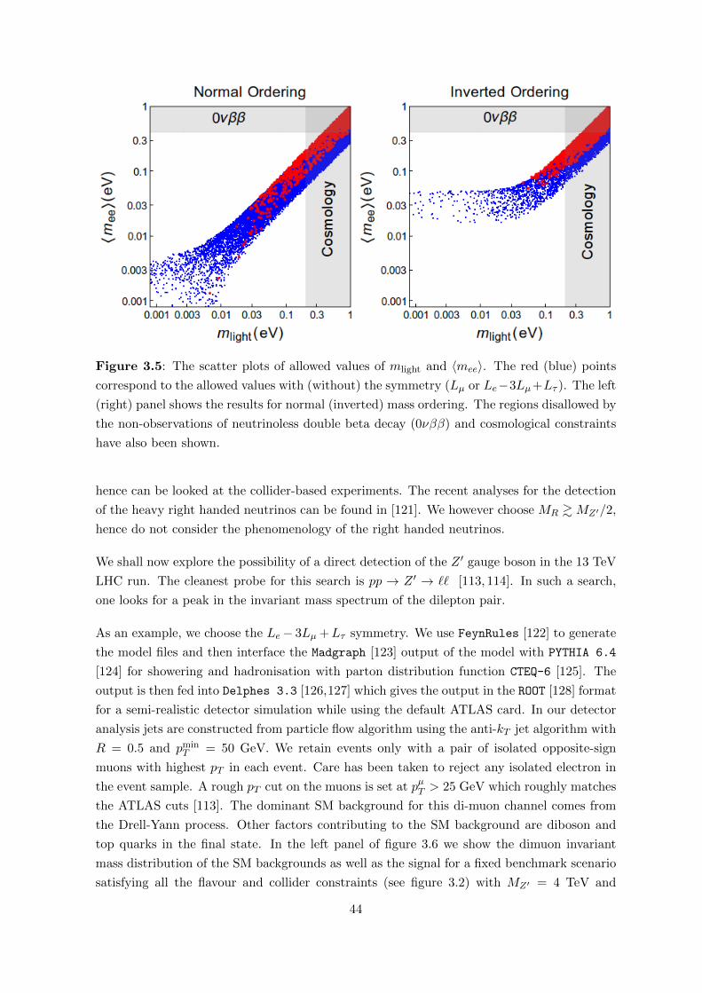
Figure 3.5: The scatter plots of allowed values of mlight and 〈mee〉. The red (blue) points
correspond to the allowed values with (without) the symmetry (Lµ or Le−3Lµ+Lτ ). The left
(right) panel shows the results for normal (inverted) mass ordering. The regions disallowed by
the non-observations of neutrinoless double beta decay (0νββ) and cosmological constraints
have also been shown.
hence can be looked at the collider-based experiments. The recent analyses for the detection
of the heavy right handed neutrinos can be found in [121]. We however choose MR &MZ′/2,
hence do not consider the phenomenology of the right handed neutrinos.
We shall now explore the possibility of a direct detection of the Z ′ gauge boson in the 13 TeV
LHC run. The cleanest probe for this search is pp → Z ′ → `` [113, 114]. In such a search,
one looks for a peak in the invariant mass spectrum of the dilepton pair.
As an example, we choose the Le− 3Lµ +Lτ symmetry. We use FeynRules [122] to generate
the model files and then interface the Madgraph [123] output of the model with PYTHIA 6.4
[124] for showering and hadronisation with parton distribution function CTEQ-6 [125]. The
output is then fed into Delphes 3.3 [126,127] which gives the output in the ROOT [128] format
for a semi-realistic detector simulation while using the default ATLAS card. In our detector
analysis jets are constructed from particle flow algorithm using the anti-kT jet algorithm with
R = 0.5 and pminT = 50 GeV. We retain events only with a pair of isolated opposite-sign
muons with highest pT in each event. Care has been taken to reject any isolated electron in
the event sample. A rough pT cut on the muons is set at pµT > 25 GeV which roughly matches
the ATLAS cuts [113]. The dominant SM background for this di-muon channel comes from
the Drell-Yann process. Other factors contributing to the SM background are diboson and
top quarks in the final state. In the left panel of figure 3.6 we show the dimuon invariant
mass distribution of the SM backgrounds as well as the signal for a fixed benchmark scenario
satisfying all the flavour and collider constraints (see figure 3.2) with MZ′ = 4 TeV and
44
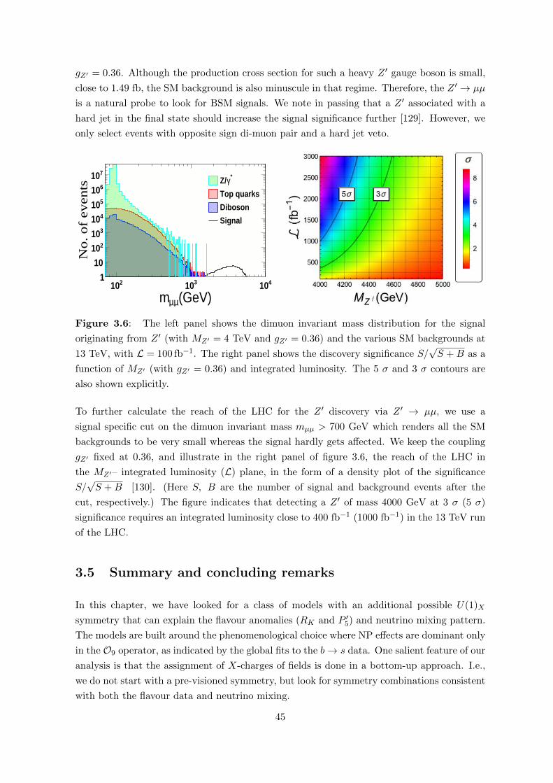
gZ′ = 0.36. Although the production cross section for such a heavy Z ′ gauge boson is small,
close to 1.49 fb, the SM background is also minuscule in that regime. Therefore, the Z ′ → µµ
is a natural probe to look for BSM signals. We note in passing that a Z ′ associated with a
hard jet in the final state should increase the signal significance further [129]. However, we
only select events with opposite sign di-muon pair and a hard jet veto.
(GeV)µµm210 310 410
No. of
even
ts
1
10
210
310
410
510
610
710 *γZ/
Top quarks
Diboson
Signal
Figure 3.6: The left panel shows the dimuon invariant mass distribution for the signal
originating from Z ′ (with MZ′ = 4 TeV and gZ′ = 0.36) and the various SM backgrounds at
13 TeV, with L = 100 fb−1. The right panel shows the discovery significance S/√S +B as a
function of MZ′ (with gZ′ = 0.36) and integrated luminosity. The 5 σ and 3 σ contours are
also shown explicitly.
To further calculate the reach of the LHC for the Z ′ discovery via Z ′ → µµ, we use a
signal specific cut on the dimuon invariant mass mµµ > 700 GeV which renders all the SM
backgrounds to be very small whereas the signal hardly gets affected. We keep the coupling
gZ′ fixed at 0.36, and illustrate in the right panel of figure 3.6, the reach of the LHC in
the MZ′– integrated luminosity (L) plane, in the form of a density plot of the significance
S/√S +B [130]. (Here S, B are the number of signal and background events after the
cut, respectively.) The figure indicates that detecting a Z ′ of mass 4000 GeV at 3 σ (5 σ)
significance requires an integrated luminosity close to 400 fb−1 (1000 fb−1) in the 13 TeV run
of the LHC.
3.5 Summary and concluding remarks
In this chapter, we have looked for a class of models with an additional possible U(1)X
symmetry that can explain the flavour anomalies (RK and P ′5) and neutrino mixing pattern.
The models are built around the phenomenological choice where NP effects are dominant only
in the O9 operator, as indicated by the global fits to the b→ s data. One salient feature of our
analysis is that the assignment of X-charges of fields is done in a bottom-up approach. I.e.,
we do not start with a pre-visioned symmetry, but look for symmetry combinations consistent
with both the flavour data and neutrino mixing.
45
In order to generate neutrino masses through the Type-I seesaw mechanism, we add three
right-handed neutrinos to the SM field content. This also allows us to assign vector-like
X-charges to the SM fermions, so that the anomaly cancellation can be easily achieved.
This choice also makes NP contributions to O10 and O′10 vanish. While the different X-
charge assignments to the SM generations introduce the desired element of lepton flavour
non-universality at tree level, it also introduces the problem of generating mixings in both
quark and lepton sector. This is alleviated by adding an additional doublet Higgs Φ1 that
generates the required quark mixing, and a scalar S that generates lepton mixing. The choice
of rotation matrices VuL = VuR = 1, VdL = VCKM and VdR ≈ 1 also ensures that the NP
contribution to O′9 is negligible. The scalar S also helps in avoiding the possible problem of
a Goldstone boson appearing from the breaking of a symmetry in the doublet Higgs sector.
Our model is thus rather parsimonious, with the introduction of only the two additional
scalar fields Φ1 and S. The symmetry breaking due to the vacuum expectation values of
these scalars gives mass to the new gauge boson Z ′, at the same time keeping its mixing with
the SM Z boson under control.
With the X-charges of quark and lepton generations connected through anomaly cancellation,
the X-charge assignments may be referred to in terms of the corresponding symmetries in
the lepton sector. We identify those leptonic symmetries that would give rise to the required
structure in the neutrino mass matrix, at the same time are consistent with the global fits to
the b→ s data. We find nine such symmetries, viz. Lµ−Lτ , Lµ, Le−3Lµ±Lτ , Le+3Lµ−Lτ ,
Le−Lµ±3Lτ , and Le−Lµ±Lτ . We find the allowed regions in the gZ′–MZ′ parameter space
that satisfy the bounds from neutral meson mixings, rare B decays, and direct Z ′ collider
searches.
The lepton symmetries give rise to specific textures in the right-handed neutrino mass matrix
MR, and hence, through seesaw, to patterns in the light neutrino mass matrix. The consequent
neutrino masses and mixing parameters are hence restricted by these symmetries. In order
to exemplify this, we have focussed on the symmetries Lµ and Le− 3Lµ +Lτ that give rise to
one zero-texture in MR, and are also the most favoured symmetries according to all the b→ s
global fits. We have analyzed the correlations among the CP-violating phases α1, α2, δCP, and
also explored the allowed region in the parameter space of the lightest neutrino mass mlight
and the effective neutrino mass 〈mee〉 measured in the neutrinoless double beta decay. For
Le − 3Lµ +Lτ , we also calculate the reach of the LHC for direct detection of Z ′ through the
di-muon channel. We find that discovery of Z ′ with the required mass and gauge coupling is
possible with a few hundred fb−1 integrated luminosity at the 13 TeV run.
Note that the parameters in our minimal model have been chosen such that we are in the
decoupling limit, i.e. the additional scalars H,A,H±, S, and the three right-handed neutrinos
are too heavy to affect any predictions in the model. Our model thus does not try to account
for the flavour anomalies indicated in the semileptonic b → c decays [131]. These anomalies
may be addressed in the extensions of this minimal model to include non-decoupling scenarios
(for example, where the charged Higgs is light), or additional charged W ′± gauge bosons.
46
While the former scenario needs to satisfy additional constraints from flavour and collider
data, the latter will need mechanisms for giving masses to the new gauge bosons.
In this chapter we have presented a class of symmetries that are consistent with the current
data, and not applied any aesthetic biases among them. As more data come along, some of
these symmetries are sure to be further chosen or discarded. We have chosen the symmetries
in the bottom-up approach, and have not tried to explore their possible origins. A curious
pattern applicable for some of the symmetries (Lµ, Le − 3Lµ +Lτ and Le −Lµ +Lτ ) is that
the non-universality of X-charges is displayed only by the third generation quarks and the
second generation leptons. Such patterns may provide further hints in the search for the more
fundamental theory governing the mass generation of quarks and leptons.
3.6 Afterword
In this section, we comment on the implications of including RK∗ measurements and on the
possibility of having simultaneous solutions of RK and RK∗ . In previous sections, we had
seen that most favourable solution explaining the b→ s anomalies was
CNP,µ9 ≈ −1 , CNP,e
9 ≈ 0 . (3.6.1)
This same solution, however, is unable to explain RK∗ measurement in low q2 bin. To see
this, let us note the expressions of RK and RK∗ measurements in detail [44, 133].
RK =
∫ q2max
q2min
dq2dΓ(B → Kµµ)
dq2∫ q2max
q2min
dq2dΓ(B → Kee)
dq2
, RK∗ =
∫ q2max
q2min
dq2dΓ(0+⊥)(B → K∗µµ)
dq2∫ q2max
q2min
dq2dΓ(0+⊥)(B → K∗ee)
dq2
(3.6.2)
where,
dΓ(B → K``)
dq2∝
(|C`10 + C`′10|2 +
∣∣∣∣C`9 + C`′9 +2mb
mb +mKC7fT (q2)
f+(q2)
∣∣∣∣2)
dΓ0(B → K∗``)
dq2∝
(|C`10 − C`′10|2 +
∣∣∣∣C`9 − C`′9 +2mb
mBC7T0(q2)
V0(q2)
∣∣∣∣2)
dΓ⊥(B → K∗``)
dq2∝
(|C`10|2 + |C`,′10 |2 + |C`′9 |2 +
∣∣∣∣C`9 +2mbmB
q2C7T−(q2)
V−(q2)
∣∣∣∣2)
(3.6.3)
Observing the above equations, it is certain that if we introduce a NP contribution in Cµ9 , i.e.
Cµ,NP9 , then the observables RK and RK∗ will have values lesser than their SM expectation.
However, due to photon pole enhancement of RK∗ in the low q2 bin, large negative values
of Cµ9 (much larger than -1) will be required. Such large values are undesirable for RK
measurement as they push its value outside the 2-σ range.
47
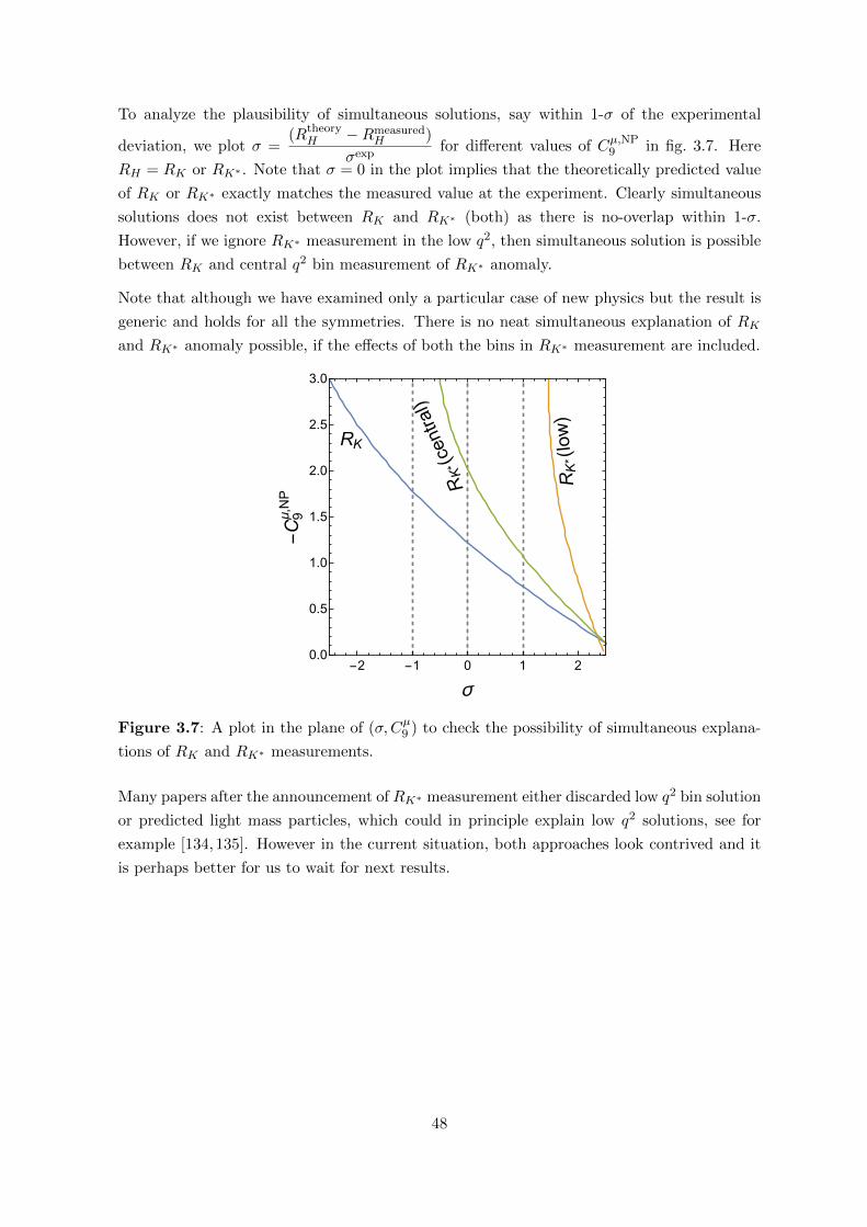
To analyze the plausibility of simultaneous solutions, say within 1-σ of the experimental
deviation, we plot σ =(Rtheory
H −RmeasuredH )
σexpfor different values of Cµ,NP
9 in fig. 3.7. Here
RH = RK or RK∗ . Note that σ = 0 in the plot implies that the theoretically predicted value
of RK or RK∗ exactly matches the measured value at the experiment. Clearly simultaneous
solutions does not exist between RK and RK∗ (both) as there is no-overlap within 1-σ.
However, if we ignore RK∗ measurement in the low q2, then simultaneous solution is possible
between RK and central q2 bin measurement of RK∗ anomaly.
Note that although we have examined only a particular case of new physics but the result is
generic and holds for all the symmetries. There is no neat simultaneous explanation of RK
and RK∗ anomaly possible, if the effects of both the bins in RK∗ measurement are included.
RK
RK*(low)
RK*(central)
-2 -1 0 1 20.0
0.5
1.0
1.5
2.0
2.5
3.0
σ
-C9μ,NP
Figure 3.7: A plot in the plane of (σ,Cµ9 ) to check the possibility of simultaneous explana-
tions of RK and RK∗ measurements.
Many papers after the announcement of RK∗ measurement either discarded low q2 bin solution
or predicted light mass particles, which could in principle explain low q2 solutions, see for
example [134, 135]. However in the current situation, both approaches look contrived and it
is perhaps better for us to wait for next results.
48
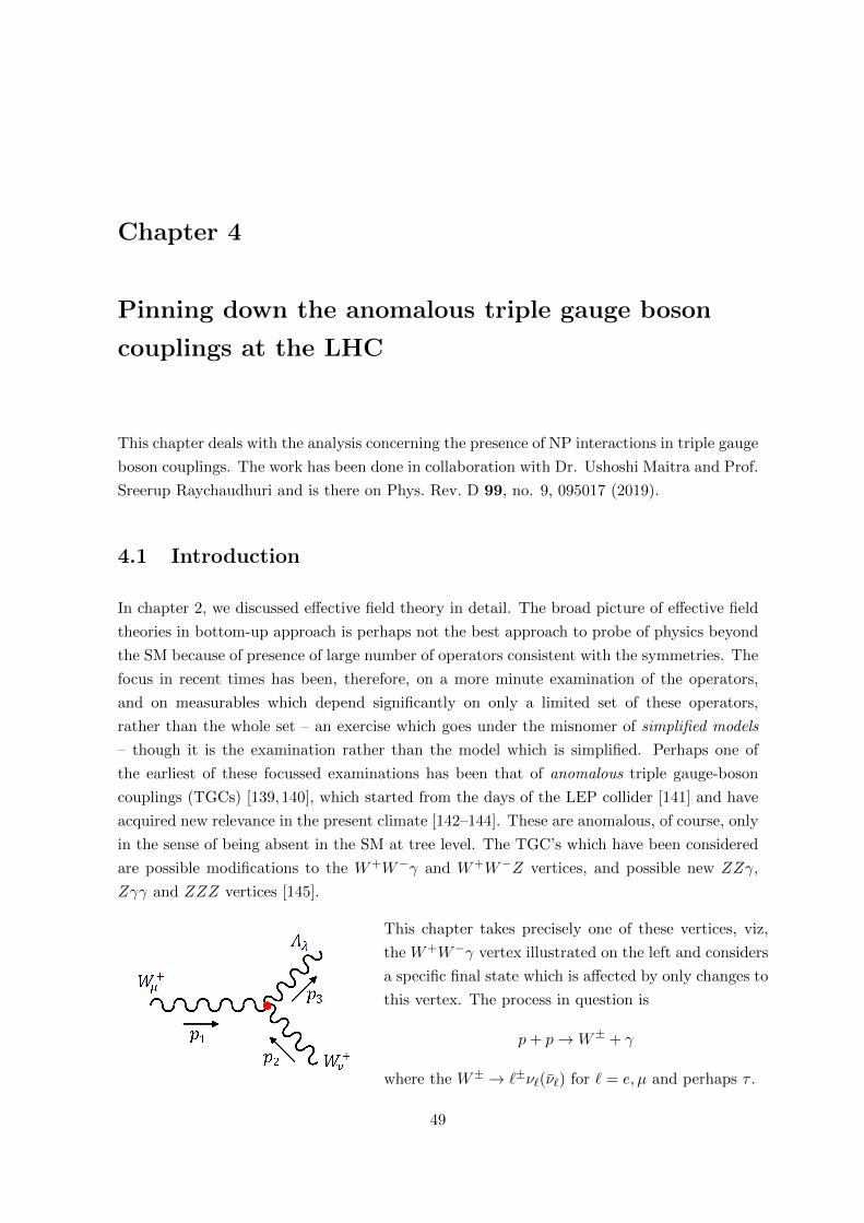
Chapter 4
Pinning down the anomalous triple gauge boson
couplings at the LHC
This chapter deals with the analysis concerning the presence of NP interactions in triple gauge
boson couplings. The work has been done in collaboration with Dr. Ushoshi Maitra and Prof.
Sreerup Raychaudhuri and is there on Phys. Rev. D 99, no. 9, 095017 (2019).
4.1 Introduction
In chapter 2, we discussed effective field theory in detail. The broad picture of effective field
theories in bottom-up approach is perhaps not the best approach to probe of physics beyond
the SM because of presence of large number of operators consistent with the symmetries. The
focus in recent times has been, therefore, on a more minute examination of the operators,
and on measurables which depend significantly on only a limited set of these operators,
rather than the whole set – an exercise which goes under the misnomer of simplified models
– though it is the examination rather than the model which is simplified. Perhaps one of
the earliest of these focussed examinations has been that of anomalous triple gauge-boson
couplings (TGCs) [139, 140], which started from the days of the LEP collider [141] and have
acquired new relevance in the present climate [142–144]. These are anomalous, of course, only
in the sense of being absent in the SM at tree level. The TGC’s which have been considered
are possible modifications to the W+W−γ and W+W−Z vertices, and possible new ZZγ,
Zγγ and ZZZ vertices [145].
This chapter takes precisely one of these vertices, viz,
the W+W−γ vertex illustrated on the left and considers
a specific final state which is affected by only changes to
this vertex. The process in question is
p+ p→W± + γ
where the W± → `±ν`(ν`) for ` = e, µ and perhaps τ .
49
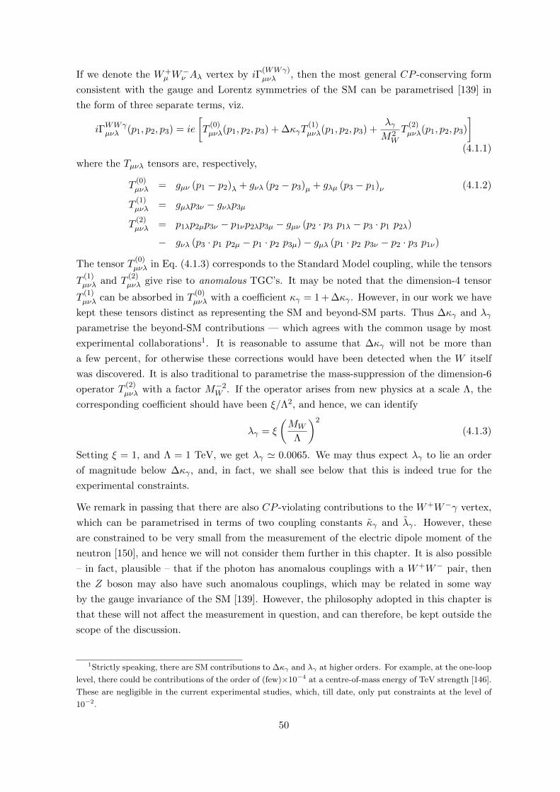
If we denote the W+µ W
−ν Aλ vertex by iΓ
(WWγ)µνλ , then the most general CP -conserving form
consistent with the gauge and Lorentz symmetries of the SM can be parametrised [139] in
the form of three separate terms, viz.
iΓWWγµνλ (p1, p2, p3) = ie
[T
(0)µνλ(p1, p2, p3) + ∆κγT
(1)µνλ(p1, p2, p3) +
λγM2W
T(2)µνλ(p1, p2, p3)
](4.1.1)
where the Tµνλ tensors are, respectively,
T(0)µνλ = gµν (p1 − p2)λ + gνλ (p2 − p3)µ + gλµ (p3 − p1)ν (4.1.2)
T(1)µνλ = gµλp3ν − gνλp3µ
T(2)µνλ = p1λp2µp3ν − p1νp2λp3µ − gµν (p2 · p3 p1λ − p3 · p1 p2λ)
− gνλ (p3 · p1 p2µ − p1 · p2 p3µ)− gµλ (p1 · p2 p3ν − p2 · p3 p1ν)
The tensor T(0)µνλ in Eq. (4.1.3) corresponds to the Standard Model coupling, while the tensors
T(1)µνλ and T
(2)µνλ give rise to anomalous TGC’s. It may be noted that the dimension-4 tensor
T(1)µνλ can be absorbed in T
(0)µνλ with a coefficient κγ = 1 + ∆κγ . However, in our work we have
kept these tensors distinct as representing the SM and beyond-SM parts. Thus ∆κγ and λγ
parametrise the beyond-SM contributions — which agrees with the common usage by most
experimental collaborations1. It is reasonable to assume that ∆κγ will not be more than
a few percent, for otherwise these corrections would have been detected when the W itself
was discovered. It is also traditional to parametrise the mass-suppression of the dimension-6
operator T(2)µνλ with a factor M−2
W . If the operator arises from new physics at a scale Λ, the
corresponding coefficient should have been ξ/Λ2, and hence, we can identify
λγ = ξ
(MW
Λ
)2
(4.1.3)
Setting ξ = 1, and Λ = 1 TeV, we get λγ ' 0.0065. We may thus expect λγ to lie an order
of magnitude below ∆κγ , and, in fact, we shall see below that this is indeed true for the
experimental constraints.
We remark in passing that there are also CP -violating contributions to the W+W−γ vertex,
which can be parametrised in terms of two coupling constants κγ and λγ . However, these
are constrained to be very small from the measurement of the electric dipole moment of the
neutron [150], and hence we will not consider them further in this chapter. It is also possible
– in fact, plausible – that if the photon has anomalous couplings with a W+W− pair, then
the Z boson may also have such anomalous couplings, which may be related in some way
by the gauge invariance of the SM [139]. However, the philosophy adopted in this chapter is
that these will not affect the measurement in question, and can therefore, be kept outside the
scope of the discussion.
1Strictly speaking, there are SM contributions to ∆κγ and λγ at higher orders. For example, at the one-loop
level, there could be contributions of the order of (few)×10−4 at a centre-of-mass energy of TeV strength [146].
These are negligible in the current experimental studies, which, till date, only put constraints at the level of
10−2.
50
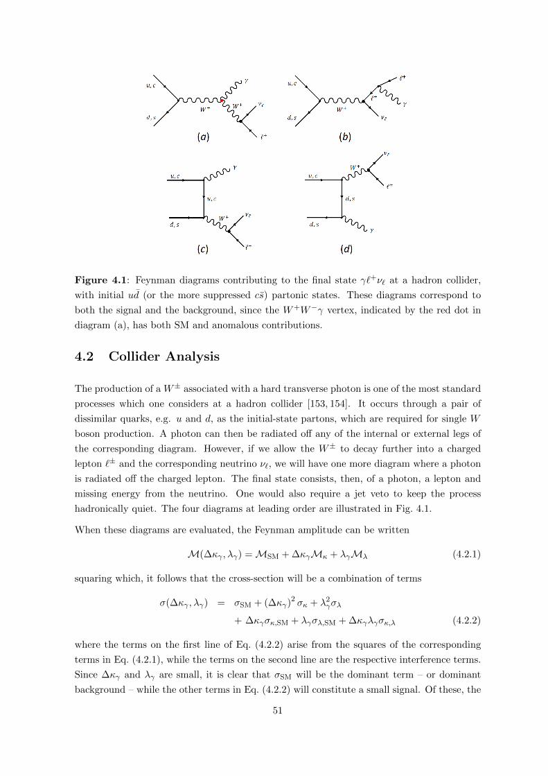
Figure 4.1: Feynman diagrams contributing to the final state γ`+ν` at a hadron collider,
with initial ud (or the more suppressed cs) partonic states. These diagrams correspond to
both the signal and the background, since the W+W−γ vertex, indicated by the red dot in
diagram (a), has both SM and anomalous contributions.
4.2 Collider Analysis
The production of a W± associated with a hard transverse photon is one of the most standard
processes which one considers at a hadron collider [153, 154]. It occurs through a pair of
dissimilar quarks, e.g. u and d, as the initial-state partons, which are required for single W
boson production. A photon can then be radiated off any of the internal or external legs of
the corresponding diagram. However, if we allow the W± to decay further into a charged
lepton `± and the corresponding neutrino ν`, we will have one more diagram where a photon
is radiated off the charged lepton. The final state consists, then, of a photon, a lepton and
missing energy from the neutrino. One would also require a jet veto to keep the process
hadronically quiet. The four diagrams at leading order are illustrated in Fig. 4.1.
When these diagrams are evaluated, the Feynman amplitude can be written
M(∆κγ , λγ) =MSM + ∆κγMκ + λγMλ (4.2.1)
squaring which, it follows that the cross-section will be a combination of terms
σ(∆κγ , λγ) = σSM + (∆κγ)2 σκ + λ2γσλ
+ ∆κγσκ,SM + λγσλ,SM + ∆κγλγσκ,λ (4.2.2)
where the terms on the first line of Eq. (4.2.2) arise from the squares of the corresponding
terms in Eq. (4.2.1), while the terms on the second line are the respective interference terms.
Since ∆κγ and λγ are small, it is clear that σSM will be the dominant term – or dominant
background – while the other terms in Eq. (4.2.2) will constitute a small signal. Of these, the
51
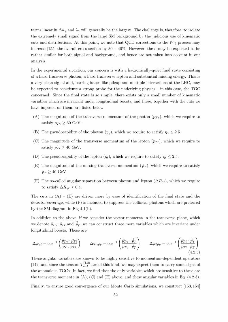
terms linear in ∆κγ and λγ will generally be the largest. The challenge is, therefore, to isolate
the extremely small signal from the large SM background by the judicious use of kinematic
cuts and distributions. At this point, we note that QCD corrections to the Wγ process may
increase [155] the overall cross-section by 30 − 40%. However, these may be expected to be
rather similar for both signal and background, and hence are not taken into account in our
analysis.
In the experimental situation, our concern is with a hadronically-quiet final state consisting
of a hard transverse photon, a hard transverse lepton and substantial missing energy. This is
a very clean signal and, barring issues like pileup and multiple interactions at the LHC, may
be expected to constitute a strong probe for the underlying physics – in this case, the TGC
concerned. Since the final state is so simple, there exists only a small number of kinematic
variables which are invariant under longitudinal boosts, and these, together with the cuts we
have imposed on them, are listed below.
(A) The magnitude of the transverse momentum of the photon (pTγ), which we require to
satisfy pTγ ≥ 60 GeV.
(B) The pseudorapidity of the photon (ηγ), which we require to satisfy ηγ ≤ 2.5.
(C) The magnitude of the transverse momentum of the lepton (pT`), which we require to
satisfy pT` ≥ 40 GeV.
(D) The pseudorapidity of the lepton (η`), which we require to satisfy η` ≤ 2.5.
(E) The magnitude of the missing transverse momentum (6pT ), which we require to satisfy
6pT ≥ 40 GeV.
(F) The so-called angular separation between photon and lepton (∆Rγ`), which we require
to satisfy ∆Rγ` ≥ 0.4.
The cuts in (A) – (E) are driven more by ease of identification of the final state and the
detector coverage, while (F) is included to suppress the collinear photons which are preferred
by the SM diagram in Fig 4.1(b).
In addition to the above, if we consider the vector momenta in the transverse plane, which
we denote ~pTγ , ~pT` and ~6pT , we can construct three more variables which are invariant under
longitudinal boosts. These are
∆ϕγ` = cos−1
(~pTγ · ~pT`pTγ pT`
)∆ϕγ 6pT = cos−1
(~pTγ · ~6pTpTγ 6pT
)∆ϕ`6pT = cos−1
(~pT` · ~6pTpT` 6pT
)(4.2.3)
These angular variables are known to be highly sensitive to momentum-dependent operators
[142] and since the tensors T(1,2)µνλ are of this kind, we may expect them to carry some signs of
the anomalous TGCs. In fact, we find that the only variables which are sensitive to these are
the transverse momenta in (A), (C) and (E) above, and these angular variables in Eq. (4.2.3).
Finally, to ensure good convergence of our Monte Carlo simulations, we construct [153, 154]
52
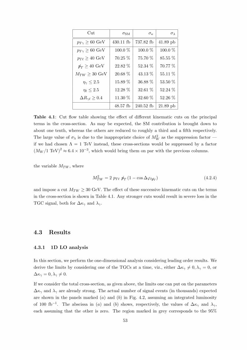
Cut σSM σκ σλ
pTγ ≥ 60 GeV 430.11 fb 737.82 fb 41.89 pb
pTγ ≥ 60 GeV 100.0 % 100.0 % 100.0 %
pT` ≥ 40 GeV 70.25 % 75.70 % 85.55 %
6pT ≥ 40 GeV 22.82 % 52.34 % 70.77 %
MTW ≥ 30 GeV 20.68 % 43.13 % 55.11 %
ηγ ≤ 2.5 15.89 % 36.88 % 53.50 %
η` ≤ 2.5 12.28 % 32.61 % 52.24 %
∆Rγ` ≥ 0.4 11.30 % 32.60 % 52.26 %
48.57 fb 240.52 fb 21.89 pb
Table 4.1: Cut flow table showing the effect of different kinematic cuts on the principal
terms in the cross-section. As may be expected, the SM contribution is brought down to
about one tenth, whereas the others are reduced to roughly a third and a fifth respectively.
The large value of σλ is due to the inappropriate choice of M2W as the suppression factor —
if we had chosen Λ = 1 TeV instead, these cross-sections would be suppressed by a factor
(MW /1 TeV)2 ≈ 6.4× 10⁻³, which would bring them on par with the previous columns.
the variable MTW , where
M2TW = 2 pT` 6pT (1− cos ∆ϕ`6pT ) (4.2.4)
and impose a cut MTW ≥ 30 GeV. The effect of these successive kinematic cuts on the terms
in the cross-section is shown in Table 4.1. Any stronger cuts would result in severe loss in the
TGC signal, both for ∆κγ and λγ .
4.3 Results
4.3.1 1D LO analysis
In this section, we perform the one-dimensional analysis considering leading order results. We
derive the limits by considering one of the TGCs at a time, viz., either ∆κγ 6= 0, λγ = 0, or
∆κγ = 0, λγ 6= 0.
If we consider the total cross-section, as given above, the limits one can put on the parameters
∆κγ and λγ are already strong. The actual number of signal events (in thousands) expected
are shown in the panels marked (a) and (b) in Fig. 4.2, assuming an integrated luminosity
of 100 fb−1. The abscissa in (a) and (b) shows, respectively, the values of ∆κγ and λγ ,
each assuming that the other is zero. The region marked in grey corresponds to the 95%
53
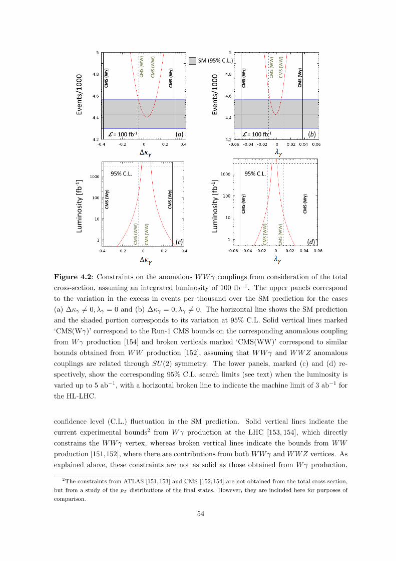
Lum
ino
sity
[fb
-1]
Lum
ino
sity
[fb
-1]
Eve
nts
/10
00
Eve
nts
/10
00
𝓛 = 100 fb-1 𝓛 = 100 fb-1
95% C.L. 95% C.L.
CM
S (W
W)
CM
S (W
W)
CM
S (W
W)
CM
S (W
W)
CM
S (W
W)
CM
S (W
W)
CM
S (W
W)
CM
S (W
W)
CM
S (W
g)
CM
S (W
g)
CM
S (W
g)
CM
S (W
g)
CM
S (W
g)
CM
S (W
g)
CM
S (W
g)
CM
S (W
g)
(a) (b)
(c) (d)
SM (95% C.L.)
Figure 4.2: Constraints on the anomalous WWγ couplings from consideration of the total
cross-section, assuming an integrated luminosity of 100 fb−1. The upper panels correspond
to the variation in the excess in events per thousand over the SM prediction for the cases
(a) ∆κγ 6= 0, λγ = 0 and (b) ∆κγ = 0, λγ 6= 0. The horizontal line shows the SM prediction
and the shaded portion corresponds to its variation at 95% C.L. Solid vertical lines marked
‘CMS(Wγ)’ correspond to the Run-1 CMS bounds on the corresponding anomalous coupling
from Wγ production [154] and broken verticals marked ‘CMS(WW)’ correspond to similar
bounds obtained from WW production [152], assuming that WWγ and WWZ anomalous
couplings are related through SU(2) symmetry. The lower panels, marked (c) and (d) re-
spectively, show the corresponding 95% C.L. search limits (see text) when the luminosity is
varied up to 5 ab−1, with a horizontal broken line to indicate the machine limit of 3 ab−1 for
the HL-LHC.
confidence level (C.L.) fluctuation in the SM prediction. Solid vertical lines indicate the
current experimental bounds2 from Wγ production at the LHC [153, 154], which directly
constrains the WWγ vertex, whereas broken vertical lines indicate the bounds from WW
production [151,152], where there are contributions from both WWγ and WWZ vertices. As
explained above, these constraints are not as solid as those obtained from Wγ production.
2The constraints from ATLAS [151,153] and CMS [152,154] are not obtained from the total cross-section,
but from a study of the pT distributions of the final states. However, they are included here for purposes of
comparison.
54
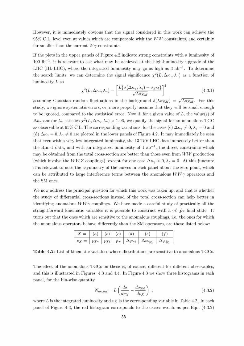
However, it is immediately obvious that the signal considered in this work can achieve the
95% C.L. level even at values which are comparable with the WW constraints, and certainly
far smaller than the current Wγ constraints.
If the plots in the upper panels of Figure 4.2 indicate strong constraints with a luminosity of
100 fb−1, it is relevant to ask what may be achieved at the high-luminosity upgrade of the
LHC (HL-LHC), where the integrated luminosity may go as high as 3 ab−1. To determine
the search limits, we can determine the signal significance χ2(L,∆κγ , λγ) as a function of
luminosity L as
χ2(L,∆κγ , λγ) =
[L{σ(∆κγ , λγ)− σSM}√
LσSM
]2
(4.3.1)
assuming Gaussian random fluctuations in the background δ(LσSM ) =√LσSM . For this
study, we ignore systematic errors, or, more properly, assume that they will be small enough
to be ignored, compared to the statistical error. Now if, for a given value of L, the value(s) of
∆κγ and/or λγ satisfies χ2(L,∆κγ , λγ) > 1.96, we qualify the signal for an anomalous TGC
as observable at 95% C.L. The corresponding variations, for the cases (c) ∆κγ 6= 0, λγ = 0 and
(d) ∆κγ = 0, λγ 6= 0 are plotted in the lower panels of Figure 4.2. It may immediately be seen
that even with a very low integrated luminosity, the 13 TeV LHC does immensely better than
the Run-1 data, and with an integrated luminosity of 1 ab−1, the direct constraints which
may be obtained from the total cross-section are better than those even from WW production
(which involve the WWZ couplings), except for one case ∆κγ > 0, λγ = 0. At this juncture
it is relevant to note the asymmetry of the curves in each panel about the zero point, which
can be attributed to large interference terms between the anomalous WWγ operators and
the SM ones.
We now address the principal question for which this work was taken up, and that is whether
the study of differential cross-sections instead of the total cross-section can help better in
identifying anomalous WWγ couplings. We have made a careful study of practically all the
straightforward kinematic variables it is possible to construct with a γ` 6 pT final state. It
turns out that the ones which are sensitive to the anomalous couplings, i.e. the ones for which
the anomalous operators behave differently than the SM operators, are those listed below:
X = (a) (b) (c) (d) (e) (f)
vX = pTγ pT` 6pT ∆ϕγ` ∆ϕγ 6pT ∆ϕ`6pT
Table 4.2: List of kinematic variables whose distributions are sensitive to anomalous TGCs.
The effect of the anomalous TGCs on these is, of course, different for different observables,
and this is illustrated in Figures 4.3 and 4.4. In Figure 4.3 we show three histograms in each
panel, for the bin-wise quantity
Nexcess = L
(dσ
dvX− dσSM
dvX
), (4.3.2)
where L is the integrated luminosity and vX is the corresponding variable in Table 4.2. In each
panel of Figure 4.3, the red histogram corresponds to the excess events as per Eqn. (4.3.2)
55
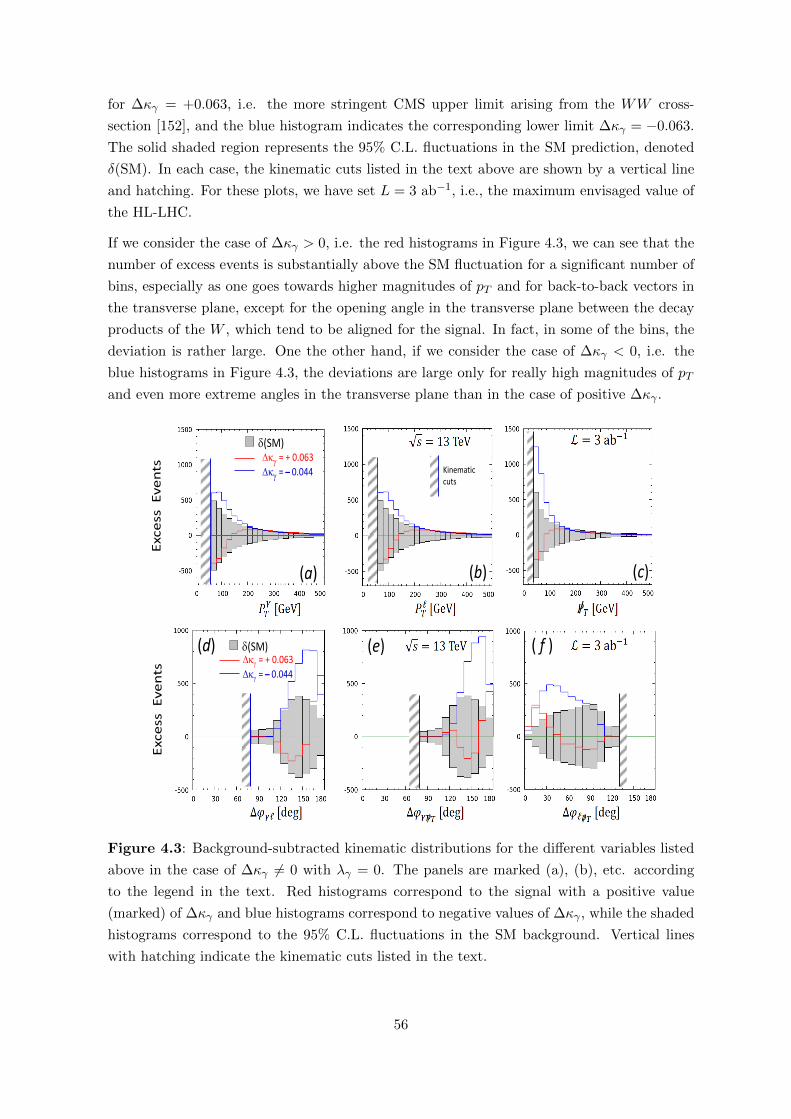
for ∆κγ = +0.063, i.e. the more stringent CMS upper limit arising from the WW cross-
section [152], and the blue histogram indicates the corresponding lower limit ∆κγ = −0.063.
The solid shaded region represents the 95% C.L. fluctuations in the SM prediction, denoted
δ(SM). In each case, the kinematic cuts listed in the text above are shown by a vertical line
and hatching. For these plots, we have set L = 3 ab−1, i.e., the maximum envisaged value of
the HL-LHC.
If we consider the case of ∆κγ > 0, i.e. the red histograms in Figure 4.3, we can see that the
number of excess events is substantially above the SM fluctuation for a significant number of
bins, especially as one goes towards higher magnitudes of pT and for back-to-back vectors in
the transverse plane, except for the opening angle in the transverse plane between the decay
products of the W , which tend to be aligned for the signal. In fact, in some of the bins, the
deviation is rather large. One the other hand, if we consider the case of ∆κγ < 0, i.e. the
blue histograms in Figure 4.3, the deviations are large only for really high magnitudes of pT
and even more extreme angles in the transverse plane than in the case of positive ∆κγ .
Exc
ess
E
ve
nts
E
xce
ss E
ve
nts
/
/ /
(a) (b) (c)
(e) ( f ) (d)
d(SM) Dkg = + 0.063
Dkg = 0.044
d(SM) Dkg = + 0.063
Dkg = 0.044
Kinematic cuts
Figure 4.3: Background-subtracted kinematic distributions for the different variables listed
above in the case of ∆κγ 6= 0 with λγ = 0. The panels are marked (a), (b), etc. according
to the legend in the text. Red histograms correspond to the signal with a positive value
(marked) of ∆κγ and blue histograms correspond to negative values of ∆κγ , while the shaded
histograms correspond to the 95% C.L. fluctuations in the SM background. Vertical lines
with hatching indicate the kinematic cuts listed in the text.
56
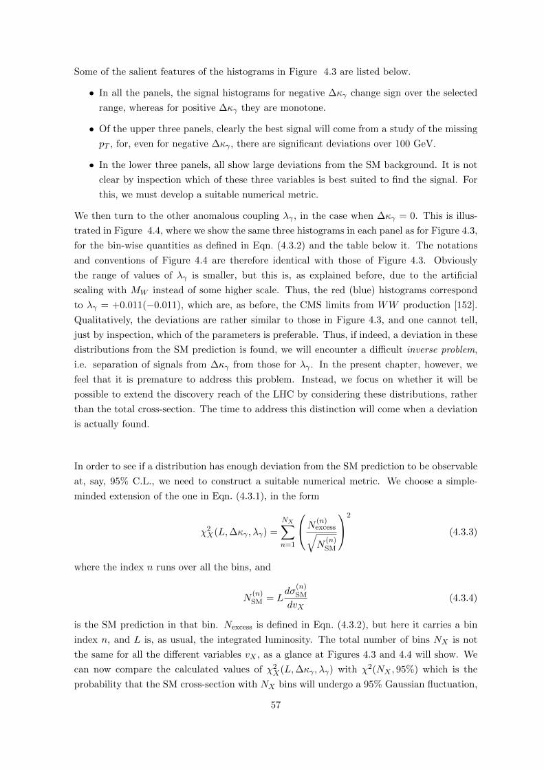
Some of the salient features of the histograms in Figure 4.3 are listed below.
• In all the panels, the signal histograms for negative ∆κγ change sign over the selected
range, whereas for positive ∆κγ they are monotone.
• Of the upper three panels, clearly the best signal will come from a study of the missing
pT , for, even for negative ∆κγ , there are significant deviations over 100 GeV.
• In the lower three panels, all show large deviations from the SM background. It is not
clear by inspection which of these three variables is best suited to find the signal. For
this, we must develop a suitable numerical metric.
We then turn to the other anomalous coupling λγ , in the case when ∆κγ = 0. This is illus-
trated in Figure 4.4, where we show the same three histograms in each panel as for Figure 4.3,
for the bin-wise quantities as defined in Eqn. (4.3.2) and the table below it. The notations
and conventions of Figure 4.4 are therefore identical with those of Figure 4.3. Obviously
the range of values of λγ is smaller, but this is, as explained before, due to the artificial
scaling with MW instead of some higher scale. Thus, the red (blue) histograms correspond
to λγ = +0.011(−0.011), which are, as before, the CMS limits from WW production [152].
Qualitatively, the deviations are rather similar to those in Figure 4.3, and one cannot tell,
just by inspection, which of the parameters is preferable. Thus, if indeed, a deviation in these
distributions from the SM prediction is found, we will encounter a difficult inverse problem,
i.e. separation of signals from ∆κγ from those for λγ . In the present chapter, however, we
feel that it is premature to address this problem. Instead, we focus on whether it will be
possible to extend the discovery reach of the LHC by considering these distributions, rather
than the total cross-section. The time to address this distinction will come when a deviation
is actually found.
In order to see if a distribution has enough deviation from the SM prediction to be observable
at, say, 95% C.L., we need to construct a suitable numerical metric. We choose a simple-
minded extension of the one in Eqn. (4.3.1), in the form
χ2X(L,∆κγ , λγ) =
NX∑n=1
N(n)excess√N
(n)SM
2
(4.3.3)
where the index n runs over all the bins, and
N(n)SM = L
dσ(n)SM
dvX(4.3.4)
is the SM prediction in that bin. Nexcess is defined in Eqn. (4.3.2), but here it carries a bin
index n, and L is, as usual, the integrated luminosity. The total number of bins NX is not
the same for all the different variables vX , as a glance at Figures 4.3 and 4.4 will show. We
can now compare the calculated values of χ2X(L,∆κγ , λγ) with χ2(NX , 95%) which is the
probability that the SM cross-section with NX bins will undergo a 95% Gaussian fluctuation,
57
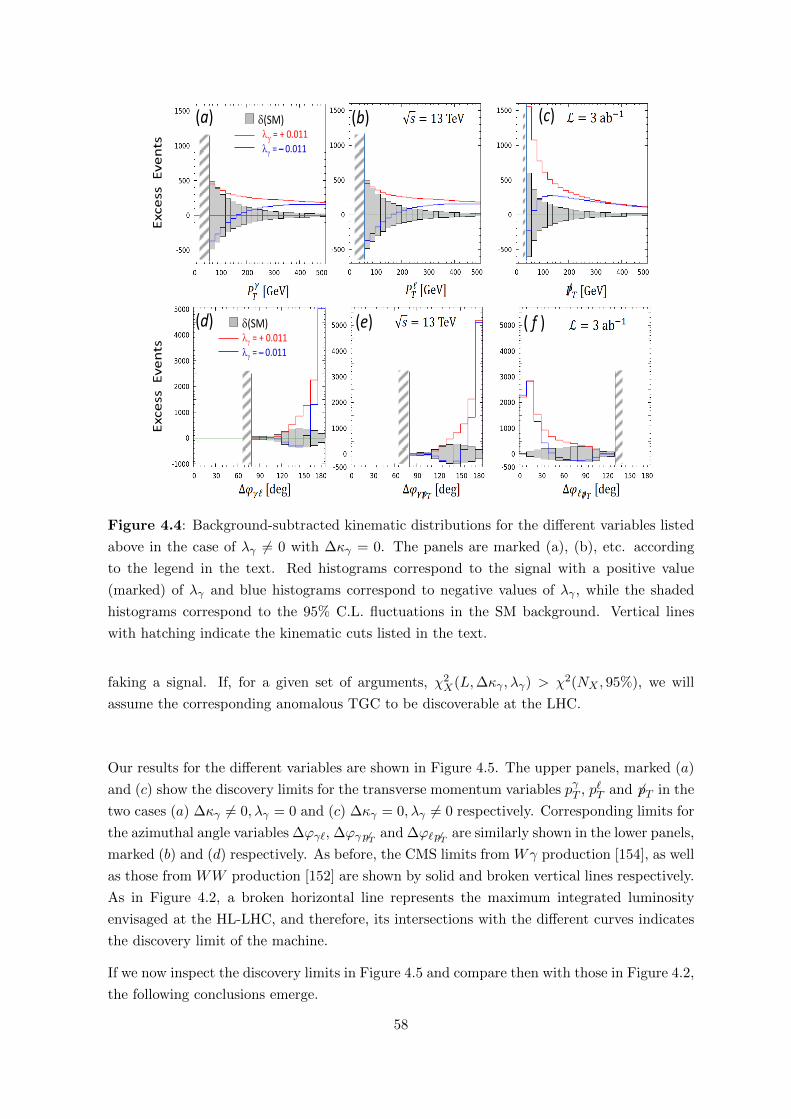
Exc
ess
E
ve
nts
E
xce
ss E
ve
nts
/
/ /
(a) (b) (c)
(e) ( f ) (d)
d(SM) lg = + 0.011
lg = 0.011
d(SM) lg = + 0.011
lg = 0.011
Figure 4.4: Background-subtracted kinematic distributions for the different variables listed
above in the case of λγ 6= 0 with ∆κγ = 0. The panels are marked (a), (b), etc. according
to the legend in the text. Red histograms correspond to the signal with a positive value
(marked) of λγ and blue histograms correspond to negative values of λγ , while the shaded
histograms correspond to the 95% C.L. fluctuations in the SM background. Vertical lines
with hatching indicate the kinematic cuts listed in the text.
faking a signal. If, for a given set of arguments, χ2X(L,∆κγ , λγ) > χ2(NX , 95%), we will
assume the corresponding anomalous TGC to be discoverable at the LHC.
Our results for the different variables are shown in Figure 4.5. The upper panels, marked (a)
and (c) show the discovery limits for the transverse momentum variables pγT , p`T and 6pT in the
two cases (a) ∆κγ 6= 0, λγ = 0 and (c) ∆κγ = 0, λγ 6= 0 respectively. Corresponding limits for
the azimuthal angle variables ∆ϕγ`, ∆ϕγ 6pT and ∆ϕ` 6pT are similarly shown in the lower panels,
marked (b) and (d) respectively. As before, the CMS limits from Wγ production [154], as well
as those from WW production [152] are shown by solid and broken vertical lines respectively.
As in Figure 4.2, a broken horizontal line represents the maximum integrated luminosity
envisaged at the HL-LHC, and therefore, its intersections with the different curves indicates
the discovery limit of the machine.
If we now inspect the discovery limits in Figure 4.5 and compare then with those in Figure 4.2,
the following conclusions emerge.
58
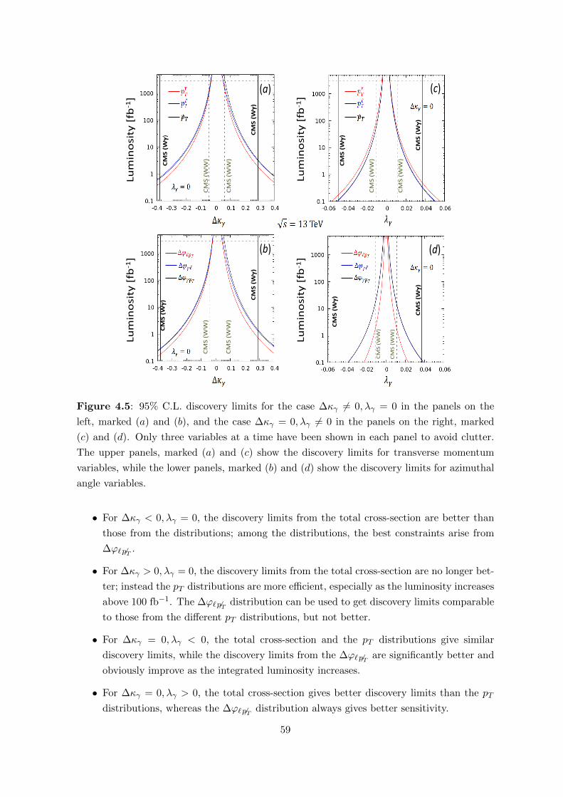
Lu
min
osi
ty [
fb-1
] Lu
min
osi
ty [
fb-1
]
Lu
min
osi
ty [
fb-1
] Lu
min
osi
ty [
fb-1
]
/ /
/
/
/
/
CM
S (
Wg) C
MS
(W
g)
CM
S (
Wg) C
MS
(W
g)
CM
S (
Wg)
CM
S (
Wg)
CM
S (
Wg)
CM
S (
WW
)
CM
S (
WW
)
CM
S (
WW
)
CM
S (
WW
)
CM
S (
WW
)
CM
S (
WW
)
CM
S (
WW
)
CM
S (
WW
)
CM
S (
Wg)
(a)
(b)
(c)
(d)
Figure 4.5: 95% C.L. discovery limits for the case ∆κγ 6= 0, λγ = 0 in the panels on the
left, marked (a) and (b), and the case ∆κγ = 0, λγ 6= 0 in the panels on the right, marked
(c) and (d). Only three variables at a time have been shown in each panel to avoid clutter.
The upper panels, marked (a) and (c) show the discovery limits for transverse momentum
variables, while the lower panels, marked (b) and (d) show the discovery limits for azimuthal
angle variables.
• For ∆κγ < 0, λγ = 0, the discovery limits from the total cross-section are better than
those from the distributions; among the distributions, the best constraints arise from
∆ϕ` 6pT .
• For ∆κγ > 0, λγ = 0, the discovery limits from the total cross-section are no longer bet-
ter; instead the pT distributions are more efficient, especially as the luminosity increases
above 100 fb−1. The ∆ϕ` 6pT distribution can be used to get discovery limits comparable
to those from the different pT distributions, but not better.
• For ∆κγ = 0, λγ < 0, the total cross-section and the pT distributions give similar
discovery limits, while the discovery limits from the ∆ϕ` 6pT are significantly better and
obviously improve as the integrated luminosity increases.
• For ∆κγ = 0, λγ > 0, the total cross-section gives better discovery limits than the pT
distributions, whereas the ∆ϕ` 6pT distribution always gives better sensitivity.
59
It is also interesting to note that of the three pT distributions, the best results are obtained
from different distributions in different regimes, whereas for the ∆ϕ distributions, ∆ϕ` 6pT is
always the most sensitive. This sensitivity is likely to be due to interference between different
helicity amplitudes [147], though that is not explicit in our calculations.
There is a very important lesson to learn from the above observations, viz., that there is no
unique variable whose study will provide the maximum sensitivity to anomalous TGCs. A
proper experimental study should, therefore, include all the variables considered above, in-
cluding the total cross-section. Currently, experimental results are mostly based on transverse
momentum studies [148,153,154], but these, as our results indicate, are not always the most
sensitive variables.
NLO analysis
As all of the above results are considered at the leading order (LO) with a fixed set of parton
distribution functions (PDFs), viz. the CTEQ-6L set, it is relevant to ask how robust these
results are against QCD effects, such as scale variation, next-to-leading order (NLO) effects
and PDF uncertainties. One could also ask whether detector effects will lead to degeneration
in the bounds obtainable from these variables. A complete analysis of these questions, we
feel, is beyond the scope of the present work, and hence we have only made some preliminary
studies in this regard.
To estimate these effects, as well as to validate our LO analyses, we have simulated the pro-
cesses in questions using a combination of the following public domain softwares: MadGraph
(version MG5-aMC-v2.4.2 [156]) to calculate cross-sections, Pythia (version Pythia8219 [157])
for the simulation including fragmentation effects and Delphes (version Delphes-3.4.1 [158]) as
a toy detector simulation. In this simulation, we trigger on a final state with a hard transverse
photon and a hard transverse lepton, with a significant amount of missing pT . In addition,
we require our process to be hadronically quiet, i.e. we put a strong jet veto.
At the very outset, let us note that with the requirement of high-pT , the detector effects,
simulated by using the Delphes package, with standard levels of smearing for the final state
photon and the lepton, are very small, and may be safely neglected. The QCD effects are sim-
ulated by running the package MadGraph, which permit (a) the inclusion of NLO corrections,
(b) variation of the factorisation scale Q, which we set to MW /2, MW and 2MW to cover the
expected range, and (c) two PDF sets, the CTEQ-6 set [159] and the NNPDF-2.3 set [160].
Even though a large portion of these are removed by the jet veto and the hard pT cuts, the
residual effects are still not small, especially for the SM background where the change can
be as much as a factor of 2. The new operators associated with the anomalous couplings
∆κγ and λγ are also changed, but by not much more than 20 - 30% after application of the
jet veto. However, all this does have an effect on the χ2. As mentioned above, a full study
of the detailed effects for all the distributions is beyond the scope of this work, though it
60
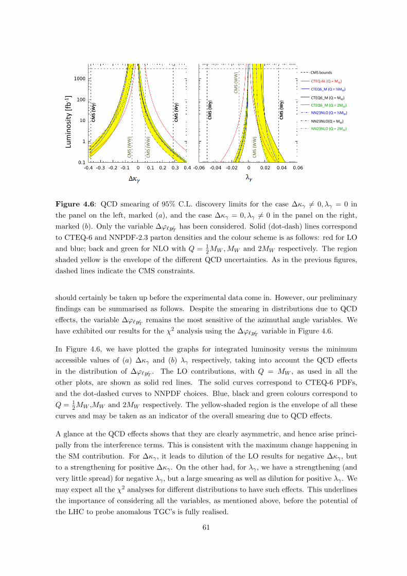
Lum
ino
sity
[fb
-1]
CM
S (W
g)
CM
S (W
g)
CM
S (W
g)
CM
S (W
g)
CM
S (W
W)
CM
S (W
W)
CM
S (W
W)
CM
S (W
W)
CTEQ-6L (Q = MW)
CTEQ6_M (Q = ½MW)
CTEQ6_M (Q = MW)
CTEQ6_M (Q = 2MW)
NN23NLO (Q = ½MW)
NN23NLO(Q = MW)
NN23NLO (Q = 2MW)
CMS bounds
Figure 4.6: QCD smearing of 95% C.L. discovery limits for the case ∆κγ 6= 0, λγ = 0 in
the panel on the left, marked (a), and the case ∆κγ = 0, λγ 6= 0 in the panel on the right,
marked (b). Only the variable ∆ϕ` 6pT has been considered. Solid (dot-dash) lines correspond
to CTEQ-6 and NNPDF-2.3 parton densities and the colour scheme is as follows: red for LO
and blue; back and green for NLO with Q = 12MW ,MW and 2MW respectively. The region
shaded yellow is the envelope of the different QCD uncertainties. As in the previous figures,
dashed lines indicate the CMS constraints.
should certainly be taken up before the experimental data come in. However, our preliminary
findings can be summarised as follows. Despite the smearing in distributions due to QCD
effects, the variable ∆ϕ` 6pT remains the most sensitive of the azimuthal angle variables. We
have exhibited our results for the χ2 analysis using the ∆ϕ` 6pT variable in Figure 4.6.
In Figure 4.6, we have plotted the graphs for integrated luminosity versus the minimum
accessible values of (a) ∆κγ and (b) λγ respectively, taking into account the QCD effects
in the distribution of ∆ϕ` 6pT . The LO contributions, with Q = MW , as used in all the
other plots, are shown as solid red lines. The solid curves correspond to CTEQ-6 PDFs,
and the dot-dashed curves to NNPDF choices. Blue, black and green colours correspond to
Q = 12MW ,MW and 2MW respectively. The yellow-shaded region is the envelope of all these
curves and may be taken as an indicator of the overall smearing due to QCD effects.
A glance at the QCD effects shows that they are clearly asymmetric, and hence arise princi-
pally from the interference terms. This is consistent with the maximum change happening in
the SM contribution. For ∆κγ , it leads to dilution of the LO results for negative ∆κγ , but
to a strengthening for positive ∆κγ . On the other had, for λγ , we have a strengthening (and
very little spread) for negative λγ , but a large smearing as well as dilution for positive λγ . We
may expect all the χ2 analyses for different distributions to have such effects. This underlines
the importance of considering all the variables, as mentioned above, before the potential of
the LHC to probe anomalous TGC’s is fully realised.
61
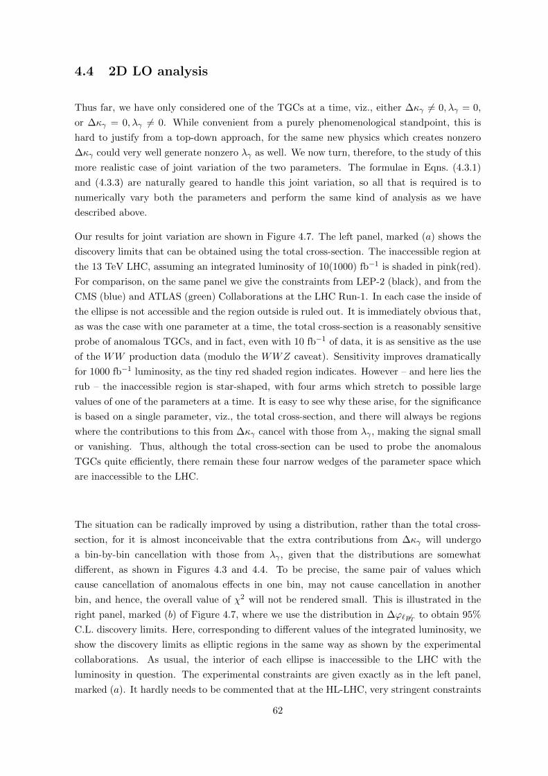
4.4 2D LO analysis
Thus far, we have only considered one of the TGCs at a time, viz., either ∆κγ 6= 0, λγ = 0,
or ∆κγ = 0, λγ 6= 0. While convenient from a purely phenomenological standpoint, this is
hard to justify from a top-down approach, for the same new physics which creates nonzero
∆κγ could very well generate nonzero λγ as well. We now turn, therefore, to the study of this
more realistic case of joint variation of the two parameters. The formulae in Eqns. (4.3.1)
and (4.3.3) are naturally geared to handle this joint variation, so all that is required is to
numerically vary both the parameters and perform the same kind of analysis as we have
described above.
Our results for joint variation are shown in Figure 4.7. The left panel, marked (a) shows the
discovery limits that can be obtained using the total cross-section. The inaccessible region at
the 13 TeV LHC, assuming an integrated luminosity of 10(1000) fb−1 is shaded in pink(red).
For comparison, on the same panel we give the constraints from LEP-2 (black), and from the
CMS (blue) and ATLAS (green) Collaborations at the LHC Run-1. In each case the inside of
the ellipse is not accessible and the region outside is ruled out. It is immediately obvious that,
as was the case with one parameter at a time, the total cross-section is a reasonably sensitive
probe of anomalous TGCs, and in fact, even with 10 fb−1 of data, it is as sensitive as the use
of the WW production data (modulo the WWZ caveat). Sensitivity improves dramatically
for 1000 fb−1 luminosity, as the tiny red shaded region indicates. However – and here lies the
rub – the inaccessible region is star-shaped, with four arms which stretch to possible large
values of one of the parameters at a time. It is easy to see why these arise, for the significance
is based on a single parameter, viz., the total cross-section, and there will always be regions
where the contributions to this from ∆κγ cancel with those from λγ , making the signal small
or vanishing. Thus, although the total cross-section can be used to probe the anomalous
TGCs quite efficiently, there remain these four narrow wedges of the parameter space which
are inaccessible to the LHC.
The situation can be radically improved by using a distribution, rather than the total cross-
section, for it is almost inconceivable that the extra contributions from ∆κγ will undergo
a bin-by-bin cancellation with those from λγ , given that the distributions are somewhat
different, as shown in Figures 4.3 and 4.4. To be precise, the same pair of values which
cause cancellation of anomalous effects in one bin, may not cause cancellation in another
bin, and hence, the overall value of χ2 will not be rendered small. This is illustrated in the
right panel, marked (b) of Figure 4.7, where we use the distribution in ∆ϕ` 6pT to obtain 95%
C.L. discovery limits. Here, corresponding to different values of the integrated luminosity, we
show the discovery limits as elliptic regions in the same way as shown by the experimental
collaborations. As usual, the interior of each ellipse is inaccessible to the LHC with the
luminosity in question. The experimental constraints are given exactly as in the left panel,
marked (a). It hardly needs to be commented that at the HL-LHC, very stringent constraints
62
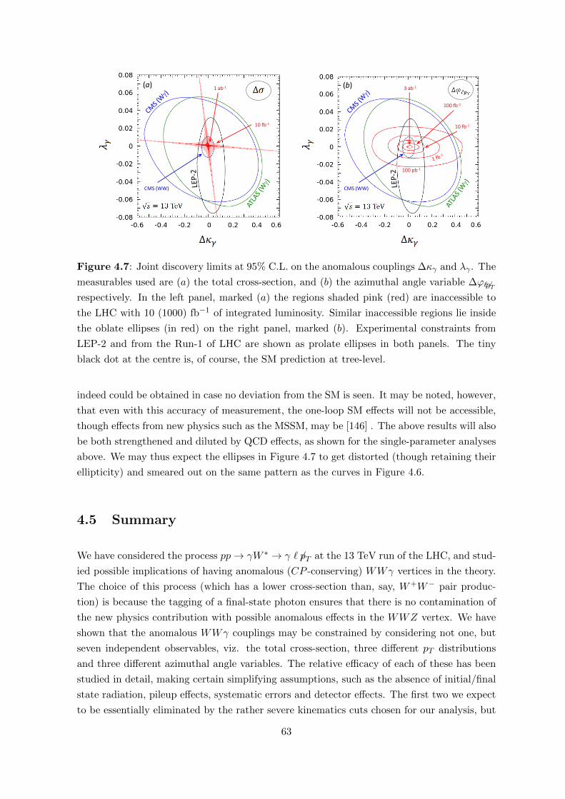
CMS (WW)
100 pb-1
10 fb-1
100 fb-1
3 ab-1
/
CMS (WW)
10 fb-1
1 ab-1 (a) (b)
Figure 4.7: Joint discovery limits at 95% C.L. on the anomalous couplings ∆κγ and λγ . The
measurables used are (a) the total cross-section, and (b) the azimuthal angle variable ∆ϕ 6pTrespectively. In the left panel, marked (a) the regions shaded pink (red) are inaccessible to
the LHC with 10 (1000) fb−1 of integrated luminosity. Similar inaccessible regions lie inside
the oblate ellipses (in red) on the right panel, marked (b). Experimental constraints from
LEP-2 and from the Run-1 of LHC are shown as prolate ellipses in both panels. The tiny
black dot at the centre is, of course, the SM prediction at tree-level.
indeed could be obtained in case no deviation from the SM is seen. It may be noted, however,
that even with this accuracy of measurement, the one-loop SM effects will not be accessible,
though effects from new physics such as the MSSM, may be [146] . The above results will also
be both strengthened and diluted by QCD effects, as shown for the single-parameter analyses
above. We may thus expect the ellipses in Figure 4.7 to get distorted (though retaining their
ellipticity) and smeared out on the same pattern as the curves in Figure 4.6.
4.5 Summary
We have considered the process pp→ γW ∗ → γ ` 6pT at the 13 TeV run of the LHC, and stud-
ied possible implications of having anomalous (CP -conserving) WWγ vertices in the theory.
The choice of this process (which has a lower cross-section than, say, W+W− pair produc-
tion) is because the tagging of a final-state photon ensures that there is no contamination of
the new physics contribution with possible anomalous effects in the WWZ vertex. We have
shown that the anomalous WWγ couplings may be constrained by considering not one, but
seven independent observables, viz. the total cross-section, three different pT distributions
and three different azimuthal angle variables. The relative efficacy of each of these has been
studied in detail, making certain simplifying assumptions, such as the absence of initial/final
state radiation, pileup effects, systematic errors and detector effects. The first two we expect
to be essentially eliminated by the rather severe kinematics cuts chosen for our analysis, but
63
the latter ones can only be estimated by a thorough experimental analysis, which is beyond
the scope of this work. Similarly, we have assumed that the kinematic cuts suggested by us
will be effective in controlling backgrounds from W + jet events (with a jet faking a photon).
Under these assumptions, we have shown that the judicious use of the variables studied, es-
pecially the azimuthal angle variable ∆ϕ` 6pT , can be used to pinpoint anomalous effects in the
process in question, to a great degree of accuracy, as the statistics collected by the LHC (and
its HL upgrade) grow larger. QCD effects will cause some dilution or strengthening of these
results, depending on the values of the TGC’s, but the overall pattern will not change too
radically. Such measurements would eventually probe not just large electoweak corrections
in the TGC sector, but could also effectively constrain new physics involving modifications
and mixings in the gauge sector. Of course, the most exciting scenario would be to see an
unambiguous deviation from the SM prediction in any of the variables (or more than one
variable) in the upcoming runs of the LHC, and it is on this hopeful note that we conclude
this chapter.
64
Chapter 5
Light CP-even Higgs Boson in type-I 2HDM at
LHC
This chapter deals with the phenomenology of a scalar lighter than the observed 125-GeV
Higgs Boson in the final states γγ and bb. The results of this chapter are based on the work:
D. Bhatia, U. Maitra and S. Niyogi, “Discovery prospects of a light Higgs boson at the LHC
in type-I 2HDM, Phys. Rev. D 97, no. 5, 055027 (2018)”. Note that most parts of the bb
analysis were performed by Dr. Ushoshi Maitra. Our analysis has become important in the
context of recent diphoton excess of 2.8σ (global 1.3 σ)in the γγ channel around 95 GeV [161].
Although at this stage, the deviation is not significant but is certainly of importance simply
because LEP had also indicated a possibility of observing an excess of Higgs-like events in
similar mass region [17].
5.1 Introduction
Despite the overwhelming success of the SM, the current measurements [21] at LHC still do
not rule out the possibility of the observed particle belonging to an enlarged scalar sector
of a beyond-SM scenario. Usually the additional scalars are considered to be heavy, and in
some cases, they are even decoupled from the low-energy effective theory. However, there
may exist scenarios where some of the new physics particles are lighter than the observed
Higgs. We explore this possibility in context of the type-1 two-Higgs-doublet model, which is
least constrained by the data.
As already discussed in Chapter. 2, two Higgs doublet models (2HDM’s) are one of the
simplest extensions of the SM with an additional scalar doublet charged under SU(2)L, where
in type-I only one of the Higgs doublets interacts with the fermions in the gauge basis. Since
the Higgs boson discovered at the LHC is CP even [162,163], amongst the five scalars predicted
in the 2HDM viz., the light CP-even scalar h, the heavier CP-even scalar H, the CP-odd
scalar A and the charged scalar H±, we can identify only one of the CP-even scalars with
the observed scalar at the LHC. Since we are interested in studying light CP-even scalar
scenarios, we identify H with the observed 125-GeV Higgs and study the phenomenology of
65
the lighter Higgs. Furthermore we choose its mass range from 70 − 110 GeV to avoid decay
of H → hh. As a result, the bounds coming from the total decay width measurement of
the observed scalar [164], the measurement of Higgs signal rate [21], and direct decay of the
observed Higgs to a pair of light Higgses, i.e., H → hh [165] becomes irrelevant in our case
(see Refs. [166,167] for an analysis with additional scalars lighter than mh/2).
To study the discovery prospects of the light CP even scalar, a suitable choice of production
and decay channels is essential. In our scenario, the light Higgs decays dominantly to bb,
except in the fermiophobic limit. Here its decay to bosons (mainly photons) becomes im-
portant. We therefore examine the light Higgs decays in the bb and γγ final states at the
LHC. Note that the search for such low mass scalars decaying to diphotons has already been
performed at LHC Run-1 [168, 169]. For the diphoton channel, we consider the production
of the scalar through gluon fusion and in association with gauge bosons. The production
of the light scalar in association with gauge boson/top pair is considered for the bb mode.
Owing to a clean environment, the diphoton final state is one of the favorite channels to
search for new resonances at the LHC. In contrast, the bb state is plagued by the huge SM
multijet backgrounds. Therefore, the light Higgs has been considered in the boosted regimes
for this channel, where the jet substructure techniques enable the efficient suppression of the
SM backgrounds [170, 171]. Note that since bb analysis was not explicitly performed by me,
I will focus only on the diphoton analysis in the chapter.
This chapter is organized in the following manner. We begin with a brief introduction to
the 2HDM in section 5.2, followed by a discussion of plausible channels which can be used
to probe the light Higgs at the LHC in section 5.3. In section 5.4, we briefly review various
constraints on the 2HDM parameter space arising from the LEP and LHC measurements, in
the context of Type-I 2HDM. A dedicated collider analysis of the light Higgs in the allowed
parameter space at the LHC is performed in section 5.5. Finally in section 5.6, we summarize
our results. Further in appendix A.1, we discuss the light Higgs couplings to diphotons. In
appendix A.2, the implications of the light charged Higgs boson on our results is analyzed,
and in appendix A.3, the tagging methods used to reconstruct boosted objects are discussed.
Finally, in appendix A.4, we tabulate the behaviour of the total cross section of the selected
modes with respect to the 2HDM parameters.
5.2 2HDM: a brief review
The Z2-symmetric 2HDM Lagrangian with two SU(2)L Higgs doublets (Φ1 and Φ2)1 can be
parametrized as [37]:
L2HDM = (DµΦ1)† DµΦ1 + (DµΦ2)† DµΦ2 + LYuk(Φ1,Φ2)− V (Φ1,Φ2) , (5.2.1)
1Under Z2 transformation, Φ1 → Φ1 and Φ2 → −Φ2
66
where LYuk represents the Yukawa interactions and V (Φ1,Φ2) is the scalar potential given as
V (Φ1,Φ2) = m211 Φ†1Φ1 +
λ1
2(Φ†1Φ1)2 +m2
22 Φ†2Φ2 +λ2
2(Φ†2Φ2)2 −
[m2
12Φ†1Φ2 + h.c]
+λ3 Φ†1Φ1 Φ†2Φ2 + λ4 Φ†1Φ2 Φ†2Φ1 −[
1
2λ5
(Φ†1Φ2
)2+H.c.
]. (5.2.2)
Here m12 is the soft Z2 symmetry-breaking parameter. Note that in our analysis, we have
assumed V (Φ1,Φ2) to be invariant under CP (i.e., charge and parity transformations) and
consequently the parameters of the scalar potential are real. The spontaneous breaking of
SU(2)L×U(1)Y symmetry results in five physical scalar fields h, H, A and H± (with masses
mh, mH , mA and mH± , respectively) and three Goldstone bosons G and G±, which appear as
the longitudinal modes for Z and W± bosons. The mass spectra of the particles are obtained
by minimizing the scalar potential V (Φ1,Φ2) in Eq. (5.2.2).
The doublets in terms of the physical fields and the Goldstone bosons can be expressed as:
Φ1 =
(G+ cosβ +H+ sinβ
1√2
[h sinα−H cosα+ i (G cosβ +A sinβ) + v1]
),
Φ2 =
(G+ sinβ −H+ cosβ
1√2
[−h cosα−H sinα+ i (G sinβ −A cosβ) + v2]
), (5.2.3)
where α and β are the rotation angles which diagonalize the mass matrices for the neutral
CP even Higgs and the charged Higgs/CP odd Higgs respectively. The parameters of the
scalar potential (m11,m22, λi ) can be expressed in terms of the rotation angles (α, β), the
Z2 symmetry breaking parameter (m12), and the masses of the scalars (mh, mH , mA, m±H)
as [37]:
m211 =
1
4
(m2h +m2
H − 4m212 tanβ +
(m2H −m2
h
)secβ cos(2α− β)
), (5.2.4)
m222 =
1
4
(m2h +m2
H − 4m212 cotβ +
(m2H −m2
h
)cscβ sin(2α− β)
), (5.2.5)
λ1 =1
2v2sec2 β
(m2h +m2
H + (m2H −m2
h) cos 2α− 2m212 tanβ
), (5.2.6)
λ2 =1
2v2csc2 β
(m2h +m2
H − (m2H −m2
h) cos 2α− 2m212 cotβ
), (5.2.7)
λ3 =1
v2csc 2β
(−2m2
12 + (m2H −m2
h) sin 2α+ 2m2H± sin 2β
), (5.2.8)
λ4 =1
v2
(m2A − 2m2
H± +m212 cscβ secβ
), (5.2.9)
λ5 =1
v2
(m2
12 cscβ secβ −m2A
), (5.2.10)
v1 = v cosβ and v2 = v sinβ . (5.2.11)
The couplings λi (i = 1, 5) are constrained by the perturbativity, vacuum stability [172], and
unitarity [173] bounds, which in turn, restrict the allowed values of the scalar masses for a
given value of α and β [37, 174]. The masses of the additional scalars also get constrained
67
from the well measured flavour and electroweak observables [175–177]. The combined effect of
these constraints on the 2HDM parameter space is discussed in appendix. A.2, in the context
of type-I 2HDM. Note that the free parameter α remains unaffected after imposition of above
constraints (see Fig. A.1 in appendix. A.2).
In our analysis, we identify the heavier CP even Higgs with the discovered scalar by fixing
mH = 125 GeV and study the phenomenology of the light CP even scalar h. At this stage
we have following free parameters — α, β, mH± , mA, m12 and mh. However, we confine
ourselves to that part of the allowed parameter space, where the masses of the charged and
pseudoscalar Higgs bosons are heavy i.e. O(500) GeV and do not affect our analysis. The
Z2 breaking parameter in this case becomes irrelevant for the light Higgs phenomenology
and can be suitably chosen to have any value less than 100 GeV (see appendix. A.2). Note
that although we have chosen the charged Higgs to be heavy for most of our analysis, we do
analyze the implications of having a low-mass charged scalar in appendix. A.2.
We now discuss the couplings of the scalar particles with fermions and gauge bosons. In the
type-I 2HDM, fermions couple only to one of the doublets i.e. Φ2 and LYuk is given as
LType−IYuk = QL YdΦ2dR +QLYuΦc
2uR +QLYeΦc2eR + h.c. ,
= −∑
f=u,d,`
mf
v
(ξfhff h+ ξfHff H − iξ
fAfγ5f A
)−√
2Vudv
u(muξ
uAPL +mdξ
dAPR
)dH+ −
√2m`
vξ`AνPR`H
+ + h.c. ,(5.2.12)
where Yu,d,e are 3 × 3 Yukawa matrices, Vud is the Cabibbo-Kobayashi-Maskawa matrix
element, mf is the mass of a fermion (f) and
ξu,d,`h = cosα/ sinβ , ξu,d,`H = sinα/ sinβ , ξuA = cotβ , ξd,`A = − cotβ . (5.2.13)
We list some of the couplings of gauge bosons with scalars that are relevant for our analysis
(see Refs. [178], [179] for a complete list):
LGauge−int =m2Z
vξVh ZµZ
µh+m2Z
vξVHZµZ
µH + 2m2W
vξVhWµW
µh+ 2m2W
vξVHWµW
µH
+αem8πv
ξγhh FµνFµν +
αem8πv
ξγH HFµνFµν , (5.2.14)
where
ξVh = sin(β − α) , ξVH = cos(β − α) , (5.2.15)
and the expressions for ξγh and ξγH are listed in appendix A.1. Based on the above couplings
of the scalars with fermions and gauge bosons, two interesting limits arise:
1. Alignment limit (α → β): Here the couplings of the heavier CP even Higgs exactly
match those of the SM Higgs.
2. Fermiophobic limit (α→ π/2) : In this limit, the tree-level couplings of the light Higgs
with fermions (ξfh) vanish [see Eq. (5.2.13)] and its loop-induced couplings with fermions
are also negligible. The light Higgs in this case behaves as a fermiophobic scalar.
68
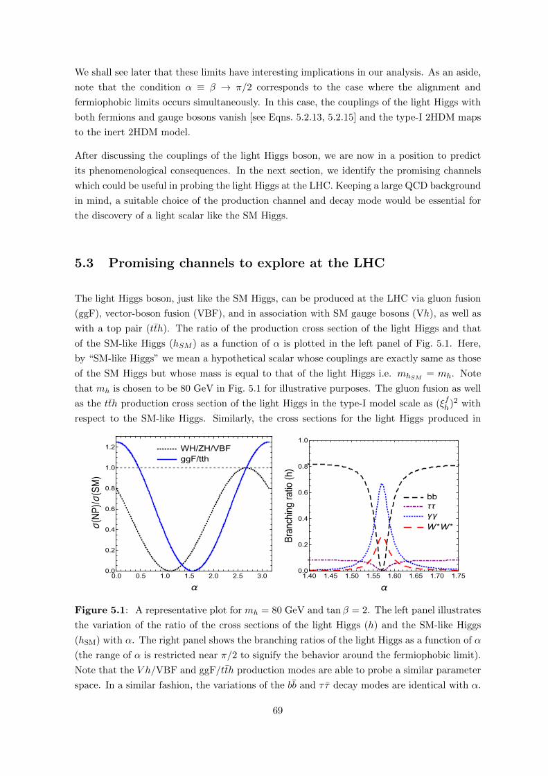
We shall see later that these limits have interesting implications in our analysis. As an aside,
note that the condition α ≡ β → π/2 corresponds to the case where the alignment and
fermiophobic limits occurs simultaneously. In this case, the couplings of the light Higgs with
both fermions and gauge bosons vanish [see Eqns. 5.2.13, 5.2.15] and the type-I 2HDM maps
to the inert 2HDM model.
After discussing the couplings of the light Higgs boson, we are now in a position to predict
its phenomenological consequences. In the next section, we identify the promising channels
which could be useful in probing the light Higgs at the LHC. Keeping a large QCD background
in mind, a suitable choice of the production channel and decay mode would be essential for
the discovery of a light scalar like the SM Higgs.
5.3 Promising channels to explore at the LHC
The light Higgs boson, just like the SM Higgs, can be produced at the LHC via gluon fusion
(ggF), vector-boson fusion (VBF), and in association with SM gauge bosons (Vh), as well as
with a top pair (tth). The ratio of the production cross section of the light Higgs and that
of the SM-like Higgs (hSM ) as a function of α is plotted in the left panel of Fig. 5.1. Here,
by “SM-like Higgs” we mean a hypothetical scalar whose couplings are exactly same as those
of the SM Higgs but whose mass is equal to that of the light Higgs i.e. mhSM = mh. Note
that mh is chosen to be 80 GeV in Fig. 5.1 for illustrative purposes. The gluon fusion as well
as the tth production cross section of the light Higgs in the type-I model scale as (ξfh)2 with
respect to the SM-like Higgs. Similarly, the cross sections for the light Higgs produced in
WH/ZH/VBF
ggF/tth
0.0 0.5 1.0 1.5 2.0 2.5 3.00.0
0.2
0.4
0.6
0.8
1.0
1.2
α
σ(NP)/σ(SM)
bb
ττγγ
W*W
*
1.40 1.45 1.50 1.55 1.60 1.65 1.70 1.750.0
0.2
0.4
0.6
0.8
1.0
α
Branchingratio
(h)
Figure 5.1: A representative plot for mh = 80 GeV and tanβ = 2. The left panel illustrates
the variation of the ratio of the cross sections of the light Higgs (h) and the SM-like Higgs
(hSM) with α. The right panel shows the branching ratios of the light Higgs as a function of α
(the range of α is restricted near π/2 to signify the behavior around the fermiophobic limit).
Note that the V h/VBF and ggF/tth production modes are able to probe a similar parameter
space. In a similar fashion, the variations of the bb and τ τ decay modes are identical with α.
69
association with gauge bosons or through vector-boson fusion scale as (ξVh )2. Therefore, the
ordinate in Fig. 5.1 essentially shows the variation of (ξih)2 against α. The scaling has been
illustrated for tanβ = 2 in Fig. 5.1. It can be seen from Eqn. (5.2.13) and (5.2.15) that for
large values of tanβ, all production channels scale identically as cos2 α.
The right panel of Fig. 5.1 represents various branching fractions of the light Higgs again as
a function of α. In most of the parameter space, the light Higgs decays dominantly to a pair
of bottom quarks. However, near α→ π/2 (the fermiophobic limit), it decays maximally to a
pair of gauge bosons. We therefore choose bb and γγ as the light Higgs decay modes for our
analysis. We must stress that the branching ratio of h to a τ pair is also significant (∼ 10%).
Since the parameter space probed by it is similar to that of bb, we restrict ourselves to the
analysis of bb in this manuscript.
Now our task is to determine the suitable production mode for a light Higgs decaying to a
pair of bottom quarks and photons. Note that analyzing bb channel in the ggF or VBF mode
is challenging due to the presence of large QCD background. However, the presence of a
lepton(s) in addition to the bb in V h or tth production modes could help to suppress these
backgrounds. Hence, we choose light Higgs production in association with a W boson and top
pair for bb analysis.2 On the other hand, the diphoton channel is one of the cleanest probes
for discovering new resonances at the LHC. This channel is also comes with the additional
advantage of enhanced sensitivity near the fermiophobic limit in the type-I 2HDM. In this
limit, i.e., α→ π/2, the decay of h to γγ becomes prominent and can only be probed through
the V h/VBF production mode as shown in Fig. 5.1. We have considered only the Wh process
in our analysis as the parameter space probed by VBF and Zh are exactly the same as that
of Wh. The diphoton channel can also be used to probe regions away from the fermiophobic
limit through ggF/tth production mode. Since the production cross section of tth is roughly
100 times smaller than that of ggF, we have not considered this for the diphoton analysis. To
summarize, we have chosen the following channels3 for probing the light Higgs at the LHC:
Channel 1: pp→ h→ γγ.
Channel 2: pp→Wh→Wγγ.
Channel 3: pp→Wh→ bb.
Channel 4: pp→ tth→ ttbb.
The phenomenological consequences of these channels will be examined in section 5.5.
5.4 Experimental constraints
In this section, we discuss the experimental constraints on the 2HDM parameter space i.e. α,
tanβ and mh from the observed Higgs signal strength measurements and the direct searches
2Zh production mode is neglected as leptonic branching ratio in case of Z is smaller than W and the
parameter space probed by Wh and Zh are exactly the same.3The behavior of the total cross section with respect to α and β corresponding to the four selected channels
is discussed in appendix A.4.
70
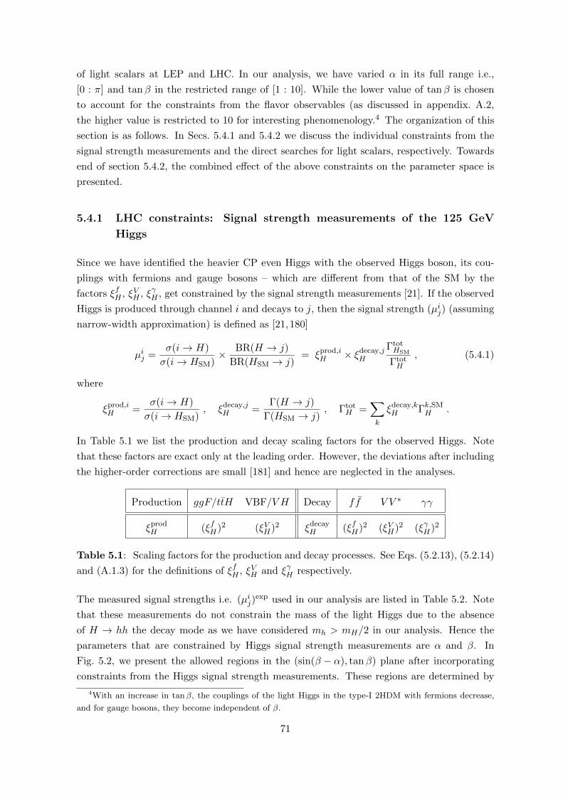
of light scalars at LEP and LHC. In our analysis, we have varied α in its full range i.e.,
[0 : π] and tanβ in the restricted range of [1 : 10]. While the lower value of tanβ is chosen
to account for the constraints from the flavor observables (as discussed in appendix. A.2,
the higher value is restricted to 10 for interesting phenomenology.4 The organization of this
section is as follows. In Secs. 5.4.1 and 5.4.2 we discuss the individual constraints from the
signal strength measurements and the direct searches for light scalars, respectively. Towards
end of section 5.4.2, the combined effect of the above constraints on the parameter space is
presented.
5.4.1 LHC constraints: Signal strength measurements of the 125 GeV
Higgs
Since we have identified the heavier CP even Higgs with the observed Higgs boson, its cou-
plings with fermions and gauge bosons – which are different from that of the SM by the
factors ξfH , ξVH , ξγH , get constrained by the signal strength measurements [21]. If the observed
Higgs is produced through channel i and decays to j, then the signal strength (µij) (assuming
narrow-width approximation) is defined as [21,180]
µij =σ(i→ H)
σ(i→ HSM)× BR(H → j)
BR(HSM → j)= ξprod,i
H × ξdecay,jH
ΓtotHSM
ΓtotH
, (5.4.1)
where
ξprod,iH =
σ(i→ H)
σ(i→ HSM), ξdecay,j
H =Γ(H → j)
Γ(HSM → j), Γtot
H =∑k
ξdecay,kH Γk,SM
H .
In Table 5.1 we list the production and decay scaling factors for the observed Higgs. Note
that these factors are exact only at the leading order. However, the deviations after including
the higher-order corrections are small [181] and hence are neglected in the analyses.
Production ggF/ttH VBF/V H Decay ff V V ∗ γγ
ξprodH (ξfH)2 (ξVH)2 ξdecay
H (ξfH)2 (ξVH)2 (ξγH)2
Table 5.1: Scaling factors for the production and decay processes. See Eqs. (5.2.13), (5.2.14)
and (A.1.3) for the definitions of ξfH , ξVH and ξγH respectively.
The measured signal strengths i.e. (µij)exp used in our analysis are listed in Table 5.2. Note
that these measurements do not constrain the mass of the light Higgs due to the absence
of H → hh the decay mode as we have considered mh > mH/2 in our analysis. Hence the
parameters that are constrained by Higgs signal strength measurements are α and β. In
Fig. 5.2, we present the allowed regions in the (sin(β − α), tanβ) plane after incorporating
constraints from the Higgs signal strength measurements. These regions are determined by
4With an increase in tanβ, the couplings of the light Higgs in the type-I 2HDM with fermions decrease,
and for gauge bosons, they become independent of β.
71
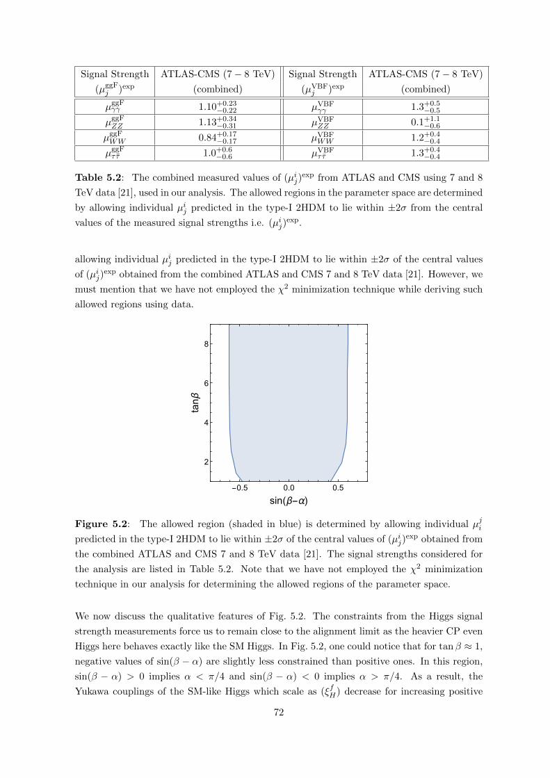
Signal Strength ATLAS-CMS (7− 8 TeV) Signal Strength ATLAS-CMS (7− 8 TeV)
(µggFj )exp (combined) (µVBF
j )exp (combined)
µggFγγ 1.10+0.23
−0.22 µVBFγγ 1.3+0.5
−0.5
µggFZZ 1.13+0.34
−0.31 µVBFZZ 0.1+1.1
−0.6
µggFWW 0.84+0.17
−0.17 µVBFWW 1.2+0.4
−0.4
µggFτ τ 1.0+0.6
−0.6 µVBFτ τ 1.3+0.4
−0.4
Table 5.2: The combined measured values of (µij)exp from ATLAS and CMS using 7 and 8
TeV data [21], used in our analysis. The allowed regions in the parameter space are determined
by allowing individual µij predicted in the type-I 2HDM to lie within ±2σ from the central
values of the measured signal strengths i.e. (µij)exp.
allowing individual µij predicted in the type-I 2HDM to lie within ±2σ of the central values
of (µij)exp obtained from the combined ATLAS and CMS 7 and 8 TeV data [21]. However, we
must mention that we have not employed the χ2 minimization technique while deriving such
allowed regions using data.
-0.5 0.0 0.5
2
4
6
8
sin(β-α)
tanβ
Figure 5.2: The allowed region (shaded in blue) is determined by allowing individual µjipredicted in the type-I 2HDM to lie within ±2σ of the central values of (µij)
exp obtained from
the combined ATLAS and CMS 7 and 8 TeV data [21]. The signal strengths considered for
the analysis are listed in Table 5.2. Note that we have not employed the χ2 minimization
technique in our analysis for determining the allowed regions of the parameter space.
We now discuss the qualitative features of Fig. 5.2. The constraints from the Higgs signal
strength measurements force us to remain close to the alignment limit as the heavier CP even
Higgs here behaves exactly like the SM Higgs. In Fig. 5.2, one could notice that for tanβ ≈ 1,
negative values of sin(β − α) are slightly less constrained than positive ones. In this region,
sin(β − α) > 0 implies α < π/4 and sin(β − α) < 0 implies α > π/4. As a result, the
Yukawa couplings of the SM-like Higgs which scale as (ξfH) decrease for increasing positive
72
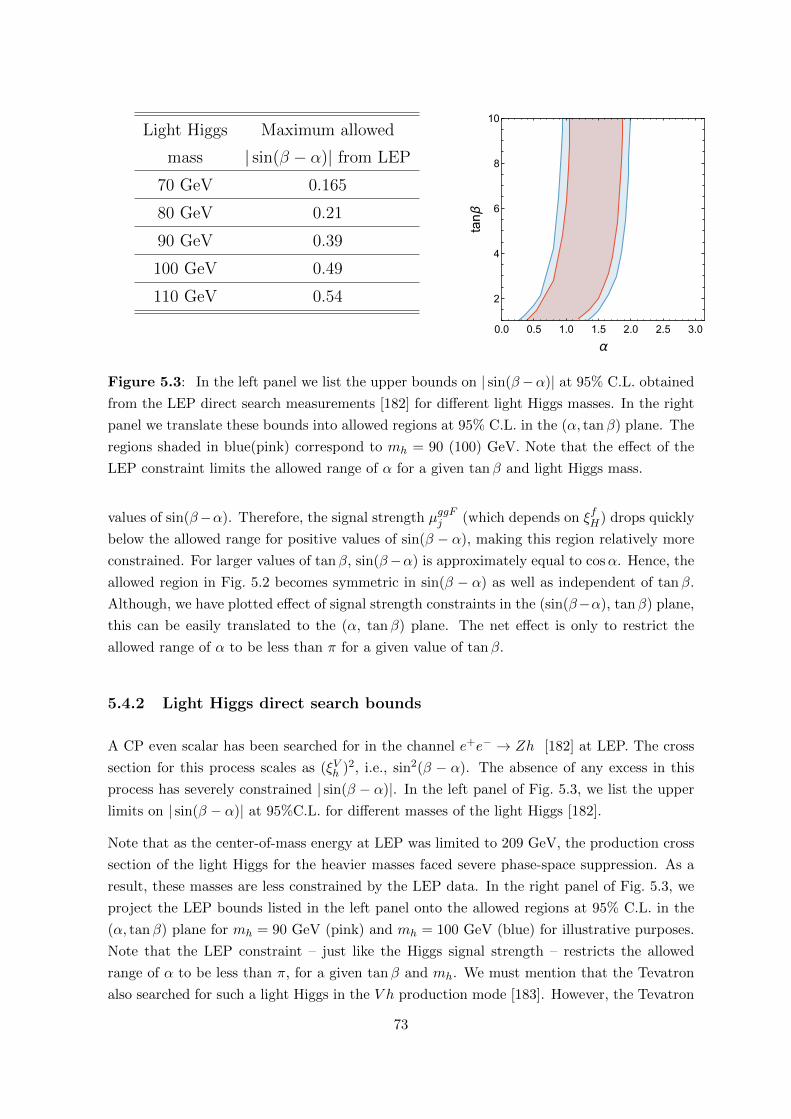
Light Higgs Maximum allowed
mass | sin(β − α)| from LEP
70 GeV 0.165
80 GeV 0.21
90 GeV 0.39
100 GeV 0.49
110 GeV 0.54
0.0 0.5 1.0 1.5 2.0 2.5 3.0
2
4
6
8
10
α
tanβ
1
Figure 5.3: In the left panel we list the upper bounds on | sin(β−α)| at 95% C.L. obtained
from the LEP direct search measurements [182] for different light Higgs masses. In the right
panel we translate these bounds into allowed regions at 95% C.L. in the (α, tanβ) plane. The
regions shaded in blue(pink) correspond to mh = 90 (100) GeV. Note that the effect of the
LEP constraint limits the allowed range of α for a given tanβ and light Higgs mass.
values of sin(β−α). Therefore, the signal strength µggFj (which depends on ξfH) drops quickly
below the allowed range for positive values of sin(β − α), making this region relatively more
constrained. For larger values of tanβ, sin(β−α) is approximately equal to cosα. Hence, the
allowed region in Fig. 5.2 becomes symmetric in sin(β − α) as well as independent of tanβ.
Although, we have plotted effect of signal strength constraints in the (sin(β−α), tanβ) plane,
this can be easily translated to the (α, tanβ) plane. The net effect is only to restrict the
allowed range of α to be less than π for a given value of tanβ.
5.4.2 Light Higgs direct search bounds
A CP even scalar has been searched for in the channel e+e− → Zh [182] at LEP. The cross
section for this process scales as (ξVh )2, i.e., sin2(β − α). The absence of any excess in this
process has severely constrained | sin(β − α)|. In the left panel of Fig. 5.3, we list the upper
limits on | sin(β − α)| at 95%C.L. for different masses of the light Higgs [182].
Note that as the center-of-mass energy at LEP was limited to 209 GeV, the production cross
section of the light Higgs for the heavier masses faced severe phase-space suppression. As a
result, these masses are less constrained by the LEP data. In the right panel of Fig. 5.3, we
project the LEP bounds listed in the left panel onto the allowed regions at 95% C.L. in the
(α, tanβ) plane for mh = 90 GeV (pink) and mh = 100 GeV (blue) for illustrative purposes.
Note that the LEP constraint – just like the Higgs signal strength – restricts the allowed
range of α to be less than π, for a given tanβ and mh. We must mention that the Tevatron
also searched for such a light Higgs in the V h production mode [183]. However, the Tevatron
73
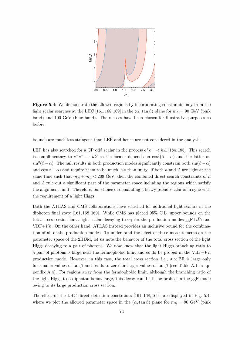
0.0 0.5 1.0 1.5 2.0 2.5 3.0
2
4
6
8
α
tanβ
Figure 5.4: We demonstrate the allowed regions by incorporating constraints only from the
light scalar searches at the LHC [161,168,169] in the (α, tanβ) plane for mh = 90 GeV (pink
band) and 100 GeV (blue band). The masses have been chosen for illustrative purposes as
before.
bounds are much less stringent than LEP and hence are not considered in the analysis.
LEP has also searched for a CP odd scalar in the process e+e− → hA [184,185]. This search
is complimentary to e+e− → hZ as the former depends on cos2(β − α) and the latter on
sin2(β−α). The null results in both production modes significantly constrain both sin(β−α)
and cos(β−α) and require them to be much less than unity. If both h and A are light at the
same time such that mA +mh < 209 GeV, then the combined direct search constraints of h
and A rule out a significant part of the parameter space including the regions which satisfy
the alignment limit. Therefore, our choice of demanding a heavy pseudoscalar is in sync with
the requirement of a light Higgs.
Both the ATLAS and CMS collaborations have searched for additional light scalars in the
diphoton final state [161, 168, 169]. While CMS has placed 95% C.L. upper bounds on the
total cross section for a light scalar decaying to γγ for the production modes ggF+tth and
VBF+V h. On the other hand, ATLAS instead provides an inclusive bound for the combina-
tion of all of the production modes. To understand the effect of these measurements on the
parameter space of the 2HDM, let us note the behavior of the total cross section of the light
Higgs decaying to a pair of photons. We now know that the light Higgs branching ratio to
a pair of photons is large near the fermiophobic limit and could be probed in the VBF+V h
production mode. However, in this case, the total cross section, i.e., σ × BR is large only
for smaller values of tanβ and tends to zero for larger values of tanβ (see Table A.1 in ap-
pendix A.4). For regions away from the fermiophobic limit, although the branching ratio of
the light Higgs to a diphoton is not large, this decay could still be probed in the ggF mode
owing to its large production cross section.
The effect of the LHC direct detection constraints [161, 168, 169] are displayed in Fig. 5.4,
where we plot the allowed parameter space in the (α, tanβ) plane for mh = 90 GeV (pink
74
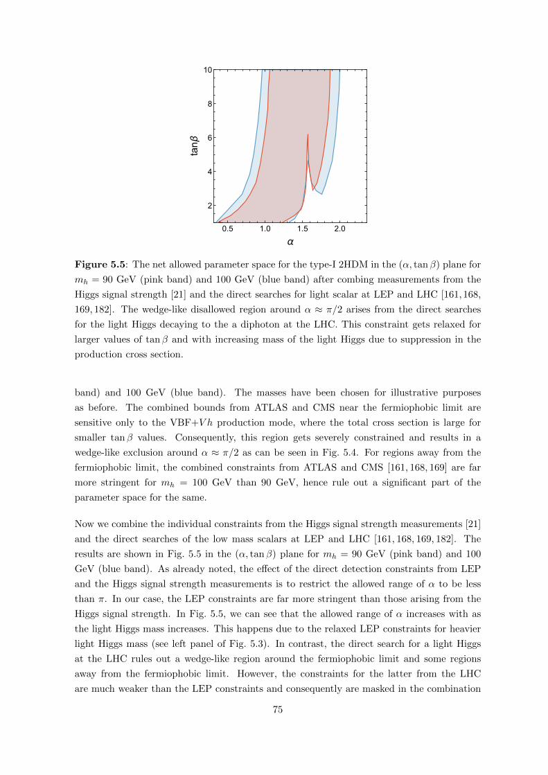
0.5 1.0 1.5 2.0
2
4
6
8
10
α
tanβ
Figure 5.5: The net allowed parameter space for the type-I 2HDM in the (α, tanβ) plane for
mh = 90 GeV (pink band) and 100 GeV (blue band) after combing measurements from the
Higgs signal strength [21] and the direct searches for light scalar at LEP and LHC [161,168,
169, 182]. The wedge-like disallowed region around α ≈ π/2 arises from the direct searches
for the light Higgs decaying to the a diphoton at the LHC. This constraint gets relaxed for
larger values of tanβ and with increasing mass of the light Higgs due to suppression in the
production cross section.
band) and 100 GeV (blue band). The masses have been chosen for illustrative purposes
as before. The combined bounds from ATLAS and CMS near the fermiophobic limit are
sensitive only to the VBF+V h production mode, where the total cross section is large for
smaller tanβ values. Consequently, this region gets severely constrained and results in a
wedge-like exclusion around α ≈ π/2 as can be seen in Fig. 5.4. For regions away from the
fermiophobic limit, the combined constraints from ATLAS and CMS [161, 168, 169] are far
more stringent for mh = 100 GeV than 90 GeV, hence rule out a significant part of the
parameter space for the same.
Now we combine the individual constraints from the Higgs signal strength measurements [21]
and the direct searches of the low mass scalars at LEP and LHC [161, 168, 169, 182]. The
results are shown in Fig. 5.5 in the (α, tanβ) plane for mh = 90 GeV (pink band) and 100
GeV (blue band). As already noted, the effect of the direct detection constraints from LEP
and the Higgs signal strength measurements is to restrict the allowed range of α to be less
than π. In our case, the LEP constraints are far more stringent than those arising from the
Higgs signal strength. In Fig. 5.5, we can see that the allowed range of α increases with as
the light Higgs mass increases. This happens due to the relaxed LEP constraints for heavier
light Higgs mass (see left panel of Fig. 5.3). In contrast, the direct search for a light Higgs
at the LHC rules out a wedge-like region around the fermiophobic limit and some regions
away from the fermiophobic limit. However, the constraints for the latter from the LHC
are much weaker than the LEP constraints and consequently are masked in the combination
75
(see Fig. 5.5). Note that the LHC constraint around the fermiophobic limit gets relaxed for
larger values of tanβ and with increasing mass of the light Higgs due to suppression in the
production cross section.
5.5 Future prospects at LHC Run-2
In this section, we discuss the prospects of observing a light Higgs boson in the following
channels: pp → h → γγ, pp → Wh → Wγγ, pp → Wh → bb, and pp → tth → ttbb.
The signal and background processes5 corresponding to each channel are generated using the
event generators Madgraph [123] or Pythia-8 [186] (depending on the number of final-state
hard particles at the parton level) with the NN23LO1 [187] parton distribution function. The
generated events are then showered and hadronized using Pythia-8. Note that the collider
analysis has been carried out in Pythia. We have not performed any detector simulation in
the analysis. We now describe the basic cuts used in our analysis.
1. A minimum cut of 20 GeV is imposed on the transverse momentum of photons, electrons,
muons, and missing energy.
2. Owing to the finite resolution of the electomagnetic calorimeter, photons and electrons
(muons) are accepted for further analysis if their pseudorapidities are less than 2.5 (2.7).
3. Photons and leptons (electrons and muons) are required to be isolated, meaning free
from the dominant jet activity in their nearby regions.
4. In experiments, there is a typical 5% probability for an electron to fake a photon, due
to track mismeasurements. Since this feature is not present in Pythia, we take this
into account in our analysis with the help of a random number. We randomly select 5%
events, where an electron is mistagged as a photon.
5. The hadrons are clustered into jets with jet radius R = 0.4 using anti-kT algorithm
[188]. The jets that satisfy — pjetT > 30 GeV and |η| < 4.5 are retained for further
analysis.
6. For the topologies which require b tagging, ∆R is computed between a b parton and
each of the anti-kT jets. If it happens to be less than 0.1, we convolute it with an
additional 70% b-tag efficiency factor.
Note that the above cuts (criteria) imposed on the final-state objects in Pythia are extremely
generic and not specific to any process under consideration. Hence these fall under the
category of preselection cuts. In the coming sections, we discuss the detailed collider analysis
5Note that there are two types of backgrounds associated with a particular signal topology: reducible and
irreducible. While the irreducible backgrounds consist of exactly the same final states, the reducible back-
grounds are somewhat different and contribute to a particular signal topology because of the misidentification
of objects.
76
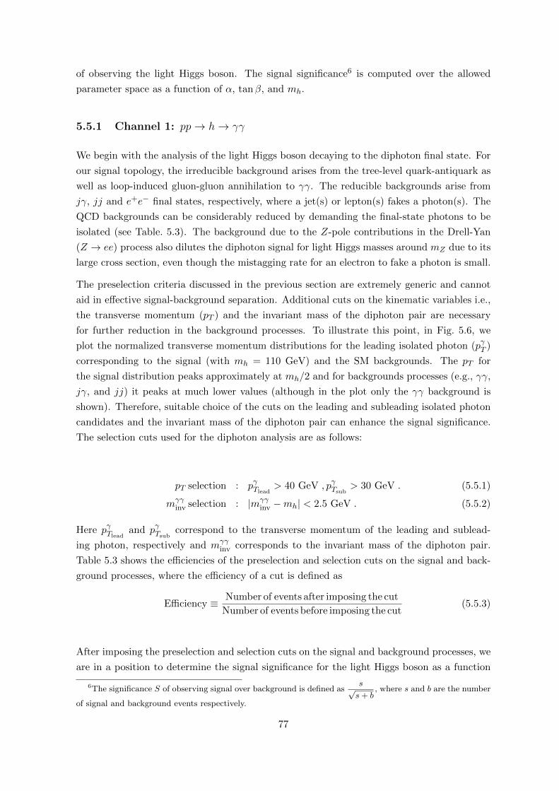
of observing the light Higgs boson. The signal significance6 is computed over the allowed
parameter space as a function of α, tanβ, and mh.
5.5.1 Channel 1: pp→ h→ γγ
We begin with the analysis of the light Higgs boson decaying to the diphoton final state. For
our signal topology, the irreducible background arises from the tree-level quark-antiquark as
well as loop-induced gluon-gluon annihilation to γγ. The reducible backgrounds arise from
jγ, jj and e+e− final states, respectively, where a jet(s) or lepton(s) fakes a photon(s). The
QCD backgrounds can be considerably reduced by demanding the final-state photons to be
isolated (see Table. 5.3). The background due to the Z-pole contributions in the Drell-Yan
(Z → ee) process also dilutes the diphoton signal for light Higgs masses around mZ due to its
large cross section, even though the mistagging rate for an electron to fake a photon is small.
The preselection criteria discussed in the previous section are extremely generic and cannot
aid in effective signal-background separation. Additional cuts on the kinematic variables i.e.,
the transverse momentum (pT ) and the invariant mass of the diphoton pair are necessary
for further reduction in the background processes. To illustrate this point, in Fig. 5.6, we
plot the normalized transverse momentum distributions for the leading isolated photon (pγT )
corresponding to the signal (with mh = 110 GeV) and the SM backgrounds. The pT for
the signal distribution peaks approximately at mh/2 and for backgrounds processes (e.g., γγ,
jγ, and jj) it peaks at much lower values (although in the plot only the γγ background is
shown). Therefore, suitable choice of the cuts on the leading and subleading isolated photon
candidates and the invariant mass of the diphoton pair can enhance the signal significance.
The selection cuts used for the diphoton analysis are as follows:
pT selection : pγTlead> 40 GeV , pγTsub
> 30 GeV . (5.5.1)
mγγinv selection : |mγγ
inv −mh| < 2.5 GeV . (5.5.2)
Here pγTleadand pγTsub
correspond to the transverse momentum of the leading and sublead-
ing photon, respectively and mγγinv corresponds to the invariant mass of the diphoton pair.
Table 5.3 shows the efficiencies of the preselection and selection cuts on the signal and back-
ground processes, where the efficiency of a cut is defined as
Efficiency ≡ Number of events after imposing the cut
Number of events before imposing the cut(5.5.3)
After imposing the preselection and selection cuts on the signal and background processes, we
are in a position to determine the signal significance for the light Higgs boson as a function
6The significance S of observing signal over background is defined ass√s+ b
, where s and b are the number
of signal and background events respectively.
77
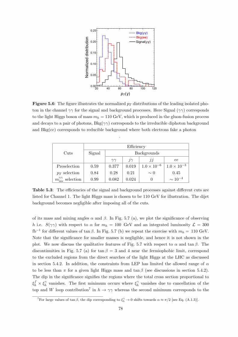
Signal(γγ)
Bkg(γγ)
Bkg(ee)
20 40 60 80 100 1200.00
0.05
0.10
0.15
0.20
0.25
pT(γ)
Normalizeddistribution
Figure 5.6: The figure illustrates the normalized pT distributions of the leading isolated pho-
ton in the channel γγ for the signal and background processes. Here Signal (γγ) corresponds
to the light Higgs boson of mass mh = 110 GeV, which is produced in the gluon-fusion process
and decays to a pair of photons, Bkg(γγ) corresponds to the irreducible diphoton background
and Bkg(ee) corresponds to reducible background where both electrons fake a photon
.
Efficiency
Cuts Signal Backgrounds
γγ jγ jj ee
Preselection 0.59 0.377 0.019 1.0× 10⁻⁶ 1.0× 10⁻³
pT selection 0.84 0.28 0.21 ∼ 0 0.45
mγγinv selection 0.99 0.082 0.024 0 ∼ 10−4
Table 5.3: The efficiencies of the signal and background processes against different cuts are
listed for Channel 1. The light Higgs mass is chosen to be 110 GeV for illustration. The dijet
background becomes negligible after imposing all of the cuts.
of its mass and mixing angles α and β. In Fig. 5.7 (a), we plot the significance of observing
h i.e. S(γγ) with respect to α for mh = 100 GeV and an integrated luminosity L = 300
fb−1 for different values of tanβ. In Fig. 5.7 (b) we repeat the exercise with mh = 110 GeV.
Note that the significance for smaller masses is negligible, and hence it is not shown in the
plot. We now discuss the qualitative features of Fig. 5.7 with respect to α and tanβ. The
discontinuities in Fig. 5.7 (a) for tanβ = 3 and 4 near the fermiophobic limit, correspond
to the excluded regions from the direct searches of the light Higgs at the LHC as discussed
in section 5.4.2. In addition, the constraints from LEP has limited the allowed range of α
to be less than π for a given light Higgs mass and tanβ (see discussions in section 5.4.2).
The dip in the significance signifies the regions where the total cross section proportional to
ξfh × ξγh vanishes. The first minimum occurs where ξγh vanishes due to cancellation of the
top and W loop contribution7 in h → γγ whereas the second minimum corresponds to the
7For large values of tanβ, the dip corresponding to ξγh → 0 shifts towards α ≈ π/2 [see Eq. (A.1.3)].
78
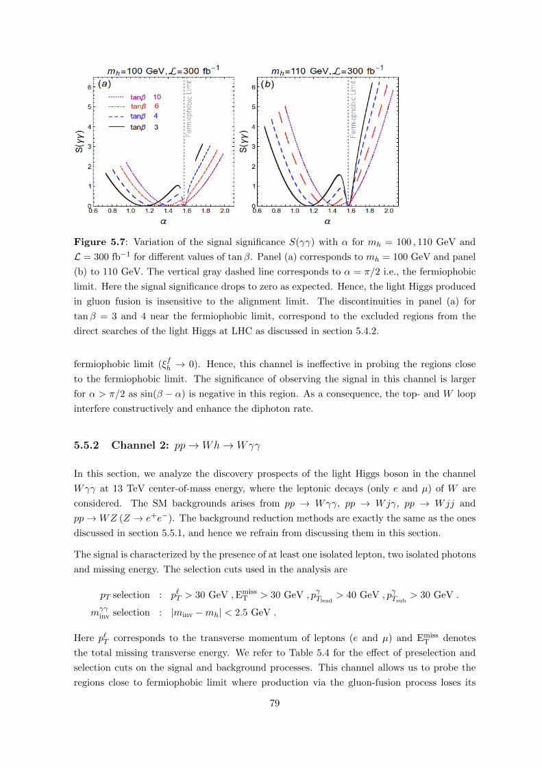
Figure 5.7: Variation of the signal significance S(γγ) with α for mh = 100 , 110 GeV and
L = 300 fb−1 for different values of tanβ. Panel (a) corresponds to mh = 100 GeV and panel
(b) to 110 GeV. The vertical gray dashed line corresponds to α = π/2 i.e., the fermiophobic
limit. Here the signal significance drops to zero as expected. Hence, the light Higgs produced
in gluon fusion is insensitive to the alignment limit. The discontinuities in panel (a) for
tanβ = 3 and 4 near the fermiophobic limit, correspond to the excluded regions from the
direct searches of the light Higgs at LHC as discussed in section 5.4.2.
fermiophobic limit (ξfh → 0). Hence, this channel is ineffective in probing the regions close
to the fermiophobic limit. The significance of observing the signal in this channel is larger
for α > π/2 as sin(β − α) is negative in this region. As a consequence, the top- and W loop
interfere constructively and enhance the diphoton rate.
5.5.2 Channel 2: pp→ Wh→ Wγγ
In this section, we analyze the discovery prospects of the light Higgs boson in the channel
Wγγ at 13 TeV center-of-mass energy, where the leptonic decays (only e and µ) of W are
considered. The SM backgrounds arises from pp → Wγγ, pp → Wjγ, pp → Wjj and
pp→WZ (Z → e+e−). The background reduction methods are exactly the same as the ones
discussed in section 5.5.1, and hence we refrain from discussing them in this section.
The signal is characterized by the presence of at least one isolated lepton, two isolated photons
and missing energy. The selection cuts used in the analysis are
pT selection : p`T > 30 GeV ,EmissT > 30 GeV , pγTlead
> 40 GeV , pγTsub> 30 GeV .
mγγinv selection : |minv −mh| < 2.5 GeV .
Here p`T corresponds to the transverse momentum of leptons (e and µ) and EmissT denotes
the total missing transverse energy. We refer to Table 5.4 for the effect of preselection and
selection cuts on the signal and background processes. This channel allows us to probe the
regions close to fermiophobic limit where production via the gluon-fusion process loses its
79
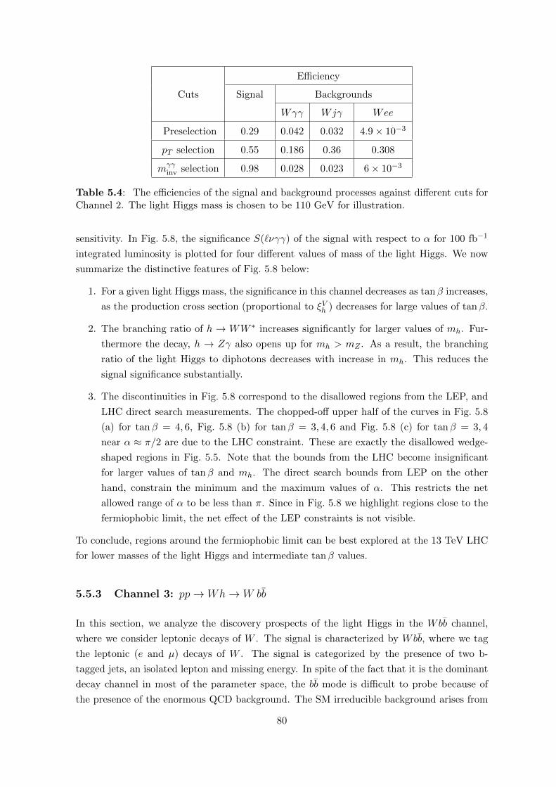
Efficiency
Cuts Signal Backgrounds
Wγγ Wjγ Wee
Preselection 0.29 0.042 0.032 4.9× 10⁻³
pT selection 0.55 0.186 0.36 0.308
mγγinv selection 0.98 0.028 0.023 6× 10⁻³
Table 5.4: The efficiencies of the signal and background processes against different cuts forChannel 2. The light Higgs mass is chosen to be 110 GeV for illustration.
sensitivity. In Fig. 5.8, the significance S(`νγγ) of the signal with respect to α for 100 fb−1
integrated luminosity is plotted for four different values of mass of the light Higgs. We now
summarize the distinctive features of Fig. 5.8 below:
1. For a given light Higgs mass, the significance in this channel decreases as tanβ increases,
as the production cross section (proportional to ξVh ) decreases for large values of tanβ.
2. The branching ratio of h → WW ∗ increases significantly for larger values of mh. Fur-
thermore the decay, h → Zγ also opens up for mh > mZ . As a result, the branching
ratio of the light Higgs to diphotons decreases with increase in mh. This reduces the
signal significance substantially.
3. The discontinuities in Fig. 5.8 correspond to the disallowed regions from the LEP, and
LHC direct search measurements. The chopped-off upper half of the curves in Fig. 5.8
(a) for tanβ = 4, 6, Fig. 5.8 (b) for tanβ = 3, 4, 6 and Fig. 5.8 (c) for tanβ = 3, 4
near α ≈ π/2 are due to the LHC constraint. These are exactly the disallowed wedge-
shaped regions in Fig. 5.5. Note that the bounds from the LHC become insignificant
for larger values of tanβ and mh. The direct search bounds from LEP on the other
hand, constrain the minimum and the maximum values of α. This restricts the net
allowed range of α to be less than π. Since in Fig. 5.8 we highlight regions close to the
fermiophobic limit, the net effect of the LEP constraints is not visible.
To conclude, regions around the fermiophobic limit can be best explored at the 13 TeV LHC
for lower masses of the light Higgs and intermediate tanβ values.
5.5.3 Channel 3: pp→ Wh→ W bb
In this section, we analyze the discovery prospects of the light Higgs in the Wbb channel,
where we consider leptonic decays of W . The signal is characterized by Wbb, where we tag
the leptonic (e and µ) decays of W . The signal is categorized by the presence of two b-
tagged jets, an isolated lepton and missing energy. In spite of the fact that it is the dominant
decay channel in most of the parameter space, the bb mode is difficult to probe because of
the presence of the enormous QCD background. The SM irreducible background arises from
80
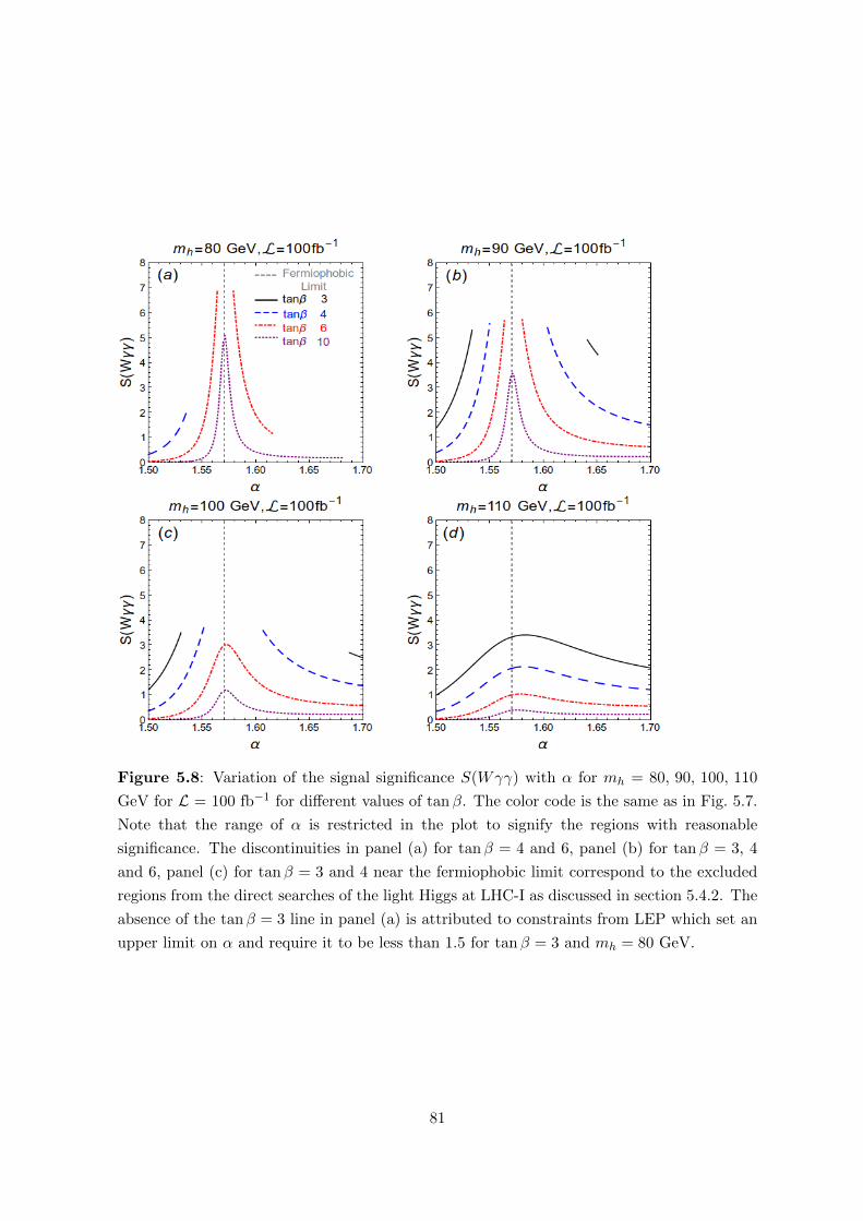
Figure 5.8: Variation of the signal significance S(Wγγ) with α for mh = 80, 90, 100, 110
GeV for L = 100 fb−1 for different values of tanβ. The color code is the same as in Fig. 5.7.
Note that the range of α is restricted in the plot to signify the regions with reasonable
significance. The discontinuities in panel (a) for tanβ = 4 and 6, panel (b) for tanβ = 3, 4
and 6, panel (c) for tanβ = 3 and 4 near the fermiophobic limit correspond to the excluded
regions from the direct searches of the light Higgs at LHC-I as discussed in section 5.4.2. The
absence of the tanβ = 3 line in panel (a) is attributed to constraints from LEP which set an
upper limit on α and require it to be less than 1.5 for tanβ = 3 and mh = 80 GeV.
81
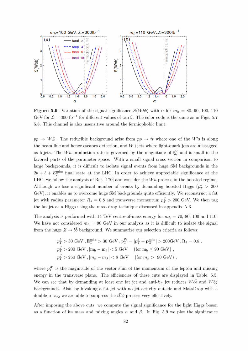
Figure 5.9: Variation of the signal significance S(Wbb) with α for mh = 80, 90, 100, 110
GeV for L = 300 fb−1 for different values of tanβ. The color code is the same as in Figs. 5.7
5.8. This channel is also insensitive around the fermiophobic limit.
pp → WZ. The reducible background arise from pp → tt where one of the W ’s is along
the beam line and hence escapes detection, and W+jets where light-quark jets are mistagged
as b-jets. The Wh production rate is governed by the magnitude of ξVh and is small in the
favored parts of the parameter space. With a small signal cross section in comparison to
large backgrounds, it is difficult to isolate signal events from huge SM backgrounds in the
2b + ` + EmissT final state at the LHC. In order to achieve appreciable significance at the
LHC, we follow the analysis of Ref. [170] and consider the Wh process in the boosted regime.
Although we lose a significant number of events by demanding boosted Higgs (phT > 200
GeV), it enables us to overcome huge SM backgrounds quite efficiently. We reconstruct a fat
jet with radius parameter RJ = 0.8 and transverse momentum pJT > 200 GeV. We then tag
the fat jet as a Higgs using the mass-drop technique discussed in appendix A.3.
The analysis is performed with 14 TeV centre-of-mass energy for mh = 70, 80, 100 and 110.
We have not considered mh = 90 GeV in our analysis as it is difficult to isolate the signal
from the huge Z → bb background. We summarize our selection criteria as follows:
p`T > 30 GeV ,EmissT > 30 GeV , pW
T = |p`T + pmissT | > 200GeV ,RJ = 0.8 ,
pJT > 200 GeV , |mh −mJ| < 5 GeV(for mh ≤ 90 GeV
),
pJT > 250 GeV , |mh −mJ | < 8 GeV(for mh > 90 GeV
),
where pWT is the magnitude of the vector sum of the momentum of the lepton and missing
energy in the transverse plane. The efficiencies of these cuts are displayed in Table. 5.5.
We can see that by demanding at least one fat jet and anti-kT jet reduces Wbb and W3j
backgrounds. Also, by invoking a fat jet with no jet activity outside and MassDrop with a
double b-tag, we are able to suppress the ttbb process very effectively.
After imposing the above cuts, we compute the signal significance for the light Higgs boson
as a function of its mass and mixing angles α and β. In Fig. 5.9 we plot the significance
82
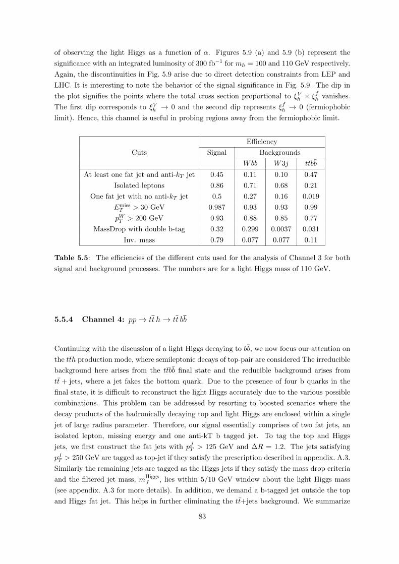
of observing the light Higgs as a function of α. Figures 5.9 (a) and 5.9 (b) represent the
significance with an integrated luminosity of 300 fb−1 for mh = 100 and 110 GeV respectively.
Again, the discontinuities in Fig. 5.9 arise due to direct detection constraints from LEP and
LHC. It is interesting to note the behavior of the signal significance in Fig. 5.9. The dip in
the plot signifies the points where the total cross section proportional to ξVh × ξfh vanishes.
The first dip corresponds to ξVh → 0 and the second dip represents ξfh → 0 (fermiophobic
limit). Hence, this channel is useful in probing regions away from the fermiophobic limit.
Efficiency
Cuts Signal Backgrounds
Wbb W3j ttbb
At least one fat jet and anti-kT jet 0.45 0.11 0.10 0.47
Isolated leptons 0.86 0.71 0.68 0.21
One fat jet with no anti-kT jet 0.5 0.27 0.16 0.019
EmissT > 30 GeV 0.987 0.93 0.93 0.99
pWT > 200 GeV 0.93 0.88 0.85 0.77
MassDrop with double b-tag 0.32 0.299 0.0037 0.031
Inv. mass 0.79 0.077 0.077 0.11
Table 5.5: The efficiencies of the different cuts used for the analysis of Channel 3 for both
signal and background processes. The numbers are for a light Higgs mass of 110 GeV.
5.5.4 Channel 4: pp→ tt h→ tt bb
Continuing with the discussion of a light Higgs decaying to bb, we now focus our attention on
the tth production mode, where semileptonic decays of top-pair are considered The irreducible
background here arises from the ttbb final state and the reducible background arises from
tt + jets, where a jet fakes the bottom quark. Due to the presence of four b quarks in the
final state, it is difficult to reconstruct the light Higgs accurately due to the various possible
combinations. This problem can be addressed by resorting to boosted scenarios where the
decay products of the hadronically decaying top and light Higgs are enclosed within a single
jet of large radius parameter. Therefore, our signal essentially comprises of two fat jets, an
isolated lepton, missing energy and one anti-kT b tagged jet. To tag the top and Higgs
jets, we first construct the fat jets with pJT > 125 GeV and ∆R = 1.2. The jets satisfying
pJT > 250 GeV are tagged as top-jet if they satisfy the prescription described in appendix. A.3.
Similarly the remaining jets are tagged as the Higgs jets if they satisfy the mass drop criteria
and the filtered jet mass, mHiggsJ , lies within 5/10 GeV window about the light Higgs mass
(see appendix. A.3 for more details). In addition, we demand a b-tagged jet outside the top
and Higgs fat jet. This helps in further eliminating the tt+jets background. We summarize
83
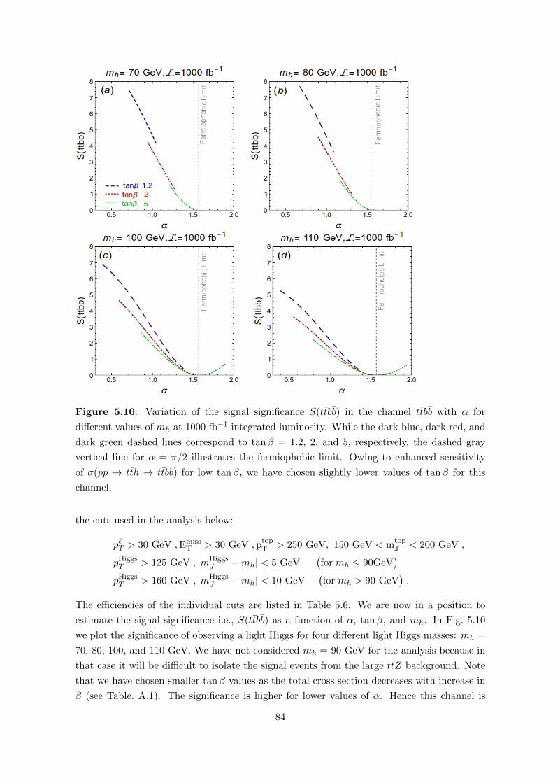
Figure 5.10: Variation of the signal significance S(ttbb) in the channel ttbb with α for
different values of mh at 1000 fb−1 integrated luminosity. While the dark blue, dark red, and
dark green dashed lines correspond to tanβ = 1.2, 2, and 5, respectively, the dashed gray
vertical line for α = π/2 illustrates the fermiophobic limit. Owing to enhanced sensitivity
of σ(pp → tth → ttbb) for low tanβ, we have chosen slightly lower values of tanβ for this
channel.
the cuts used in the analysis below:
p`T > 30 GeV ,EmissT > 30 GeV , ptop
T > 250 GeV, 150 GeV < mtopJ < 200 GeV ,
pHiggsT > 125 GeV , |mHiggs
J −mh| < 5 GeV(for mh ≤ 90GeV
)pHiggsT > 160 GeV , |mHiggs
J −mh| < 10 GeV(for mh > 90 GeV
).
The efficiencies of the individual cuts are listed in Table 5.6. We are now in a position to
estimate the signal significance i.e., S(ttbb) as a function of α, tanβ, and mh. In Fig. 5.10
we plot the significance of observing a light Higgs for four different light Higgs masses: mh =
70, 80, 100, and 110 GeV. We have not considered mh = 90 GeV for the analysis because in
that case it will be difficult to isolate the signal events from the large ttZ background. Note
that we have chosen smaller tanβ values as the total cross section decreases with increase in
β (see Table. A.1). The significance is higher for lower values of α. Hence this channel is
84
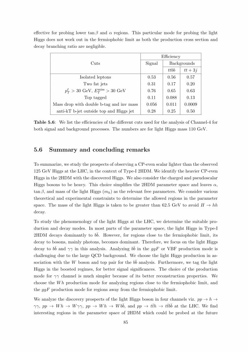
effective for probing lower tanβ and α regions. This particular mode for probing the light
Higgs does not work out in the fermiophobic limit as both the production cross section and
decay branching ratio are negligible.
Efficiency
Cuts Signal Backgrounds
ttbb tt+ 3j
Isolated leptons 0.53 0.56 0.57
Two fat jets 0.31 0.17 0.20
p`T > 30 GeV, EmissT > 30 GeV 0.76 0.65 0.63
Top tagged 0.11 0.088 0.13
Mass drop with double b-tag and inv mass 0.056 0.011 0.0009
anti-kT b-jet outside top and Higgs jet 0.28 0.25 0.50
Table 5.6: We list the efficiencies of the different cuts used for the analysis of Channel-4 for
both signal and background processes. The numbers are for light Higgs mass 110 GeV.
5.6 Summary and concluding remarks
To summarize, we study the prospects of observing a CP-even scalar lighter than the observed
125 GeV Higgs at the LHC, in the context of Type-I 2HDM. We identify the heavier CP-even
Higgs in the 2HDM with the discovered Higgs. We also consider the charged and pseudoscalar
Higgs bosons to be heavy. This choice simplifies the 2HDM parameter space and leaves α,
tanβ, and mass of the light Higgs (mh) as the relevant free parameters. We consider various
theoretical and experimental constraints to determine the allowed regions in the parameter
space. The mass of the light Higgs is taken to be greater than 62.5 GeV to avoid H → hh
decay.
To study the phenomenology of the light Higgs at the LHC, we determine the suitable pro-
duction and decay modes. In most parts of the parameter space, the light Higgs in Type-I
2HDM decays dominantly to bb. However, for regions close to the fermiophobic limit, its
decay to bosons, mainly photons, becomes dominant. Therefore, we focus on the light Higgs
decay to bb and γγ in this analysis. Analyzing bb in the ggF or VBF production mode is
challenging due to the large QCD background. We choose the light Higgs production in as-
sociation with the W boson and top pair for the bb analysis. Furthermore, we tag the light
Higgs in the boosted regimes, for better signal significances. The choice of the production
mode for γγ channel is much simpler because of its better reconstruction properties. We
choose the Wh production mode for analyzing regions close to the fermiophobic limit, and
the ggF production mode for regions away from the fermiophobic limit.
We analyze the discovery prospects of the light Higgs boson in four channels viz. pp→ h→γγ, pp → Wh → Wγγ, pp → Wh → Wbb, and pp → tth → ttbb at the LHC. We find
interesting regions in the parameter space of 2HDM which could be probed at the future
85
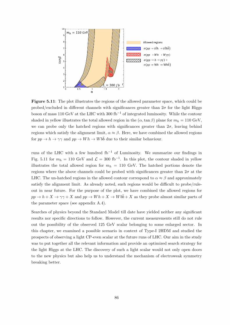
Figure 5.11: The plot illustrates the regions of the allowed parameter space, which could be
probed/excluded in different channels with significances greater than 2σ for the light Higgs
boson of mass 110 GeV at the LHC with 300 fb−1 of integrated luminosity. While the contour
shaded in yellow illustrates the total allowed region in the (α, tanβ) plane for mh = 110 GeV,
we can probe only the hatched regions with significances greater than 2σ, leaving behind
regions which satisfy the alignment limit, α ≈ β. Here, we have combined the allowed regions
for pp→ h→ γγ and pp→Wh→Wbb due to their similar behaviour.
runs of the LHC with a few hundred fb−1 of Luminosity. We summarize our findings in
Fig. 5.11 for mh = 110 GeV and L = 300 fb−1. In this plot, the contour shaded in yellow
illustrates the total allowed region for mh = 110 GeV. The hatched portions denote the
regions where the above channels could be probed with significances greater than 2σ at the
LHC. The un-hatched regions in the allowed contour correspond to α ≈ β and approximately
satisfy the alignment limit. As already noted, such regions would be difficult to probe/rule-
out in near future. For the purpose of the plot, we have combined the allowed regions for
pp→ h+X → γγ +X and pp→Wh+X →Wbb+X as they probe almost similar parts of
the parameter space (see appendix A.4).
Searches of physics beyond the Standard Model till date have yielded neither any significant
results nor specific directions to follow. However, the current measurements still do not rule
out the possibility of the observed 125 GeV scalar belonging to some enlarged sector. In
this chapter, we examined a possible scenario in context of Type-I 2HDM and studied the
prospects of observing a light CP-even scalar at the future runs of LHC. Our aim in the study
was to put together all the relevant information and provide an optimized search strategy for
the light Higgs at the LHC. The discovery of such a light scalar would not only open doors
to the new physics but also help us to understand the mechanism of electroweak symmetry
breaking better.
86
Chapter 6
Dissecting Multi-Photon Resonances at the Large
Hadron Collider
This chapter deals with the analysis concerning disentanglement of multi-photon topologies
with the diphoton ones. The work has been done in collaboration with Dr. Abhishek Iyer
and Prof. B.C. Allanach and is published in Eur. Phys. J. C 77, no. 9, 595 (2017).
6.1 Introduction
In this chapter, we consider a hypothetical new boson X, with mass around a TeV-scale,
decaying dominantly to photons, which can potentially give rise to an excess in the diphoton
final state.
There are mainly two kind of topologies which could result in such an effect viz., the standard
and the non-standard ones. In the standard case, the decay proceeds in the conventional
manner i.e. pp→ X → γγ. The non-standard topologies result in multi-photon1 final states,
but the decay products appear to be diphotons from the detector point of view. Here the
heavy resonance X decays first to lighter particles n, which further decay into diphotons,
thereby leading to a multi-photon final state. Since mn << mX , photons from n are highly
collimated and this creates an illusion of a diphoton final state in the detector.
We are interested in the disentanglement of the standard versus the non-standard topologies
in our analysis. To perform this segregation, we have ignored the SM backgrounds. For
this to be a good approximation, we require the backgrounds to be smaller than the signal
cross-section. Figure 6.1 shows viable regions for mX ≥ 1200 GeV where this is the case, i.e.
σ(pp→ X)×BR(X → γγ) is well above the background but below the current experimental
limits [34,35].
Disentanglement of the standard versus the non-standard topologies crucially depends on the
mass of the lighter resonance n. Photons deposit their energies in the electromagnetic calori-
metric cells, where the granularity of each ECAL cell is approximately 0.02×0.02 in the η−ϕ1more than two
87
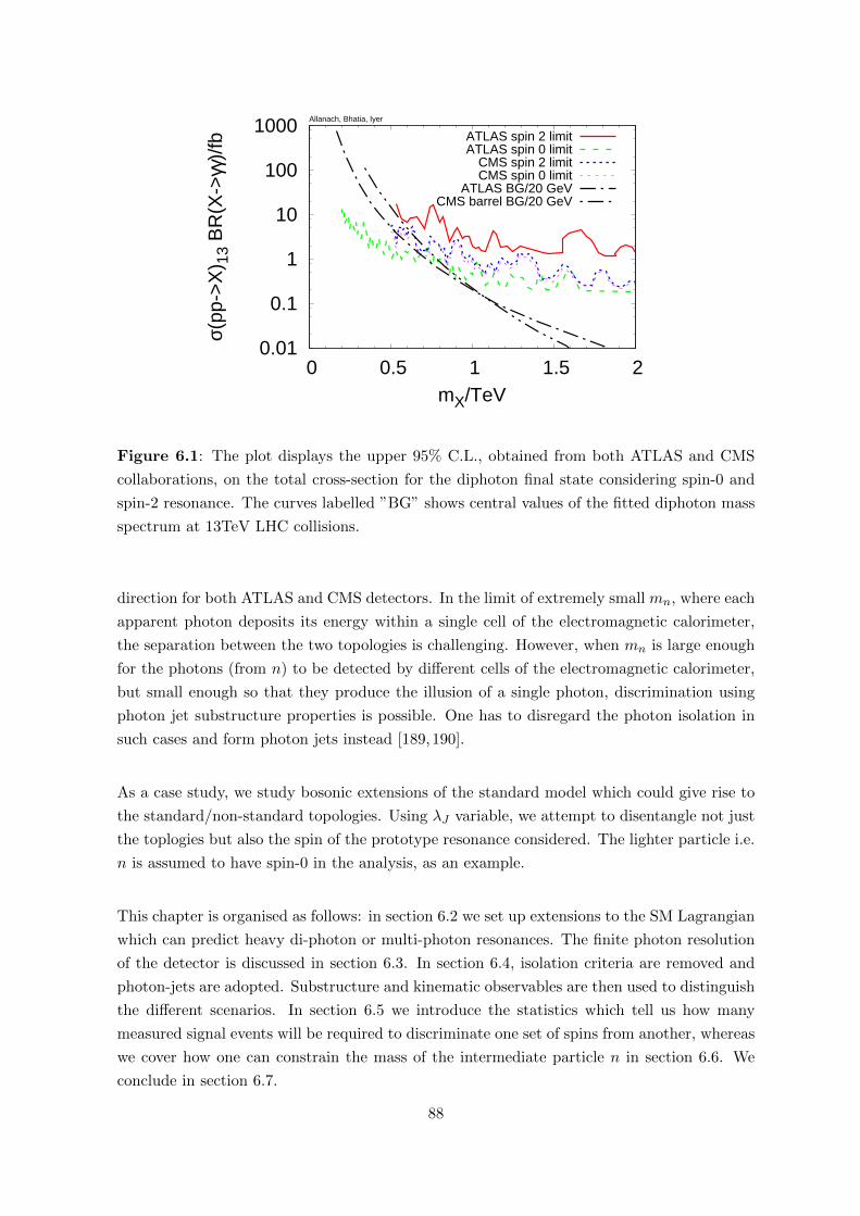
0.01
0.1
1
10
100
1000
0 0.5 1 1.5 2
Allanach, Bhatia, Iyer
σ(pp
->X
) 13
BR
(X->
γγ)/
fb
mX/TeV
ATLAS spin 2 limitATLAS spin 0 limit
CMS spin 2 limitCMS spin 0 limit
ATLAS BG/20 GeVCMS barrel BG/20 GeV
Figure 6.1: The plot displays the upper 95% C.L., obtained from both ATLAS and CMS
collaborations, on the total cross-section for the diphoton final state considering spin-0 and
spin-2 resonance. The curves labelled ”BG” shows central values of the fitted diphoton mass
spectrum at 13TeV LHC collisions.
direction for both ATLAS and CMS detectors. In the limit of extremely small mn, where each
apparent photon deposits its energy within a single cell of the electromagnetic calorimeter,
the separation between the two topologies is challenging. However, when mn is large enough
for the photons (from n) to be detected by different cells of the electromagnetic calorimeter,
but small enough so that they produce the illusion of a single photon, discrimination using
photon jet substructure properties is possible. One has to disregard the photon isolation in
such cases and form photon jets instead [189,190].
As a case study, we study bosonic extensions of the standard model which could give rise to
the standard/non-standard topologies. Using λJ variable, we attempt to disentangle not just
the toplogies but also the spin of the prototype resonance considered. The lighter particle i.e.
n is assumed to have spin-0 in the analysis, as an example.
This chapter is organised as follows: in section 6.2 we set up extensions to the SM Lagrangian
which can predict heavy di-photon or multi-photon resonances. The finite photon resolution
of the detector is discussed in section 6.3. In section 6.4, isolation criteria are removed and
photon-jets are adopted. Substructure and kinematic observables are then used to distinguish
the different scenarios. In section 6.5 we introduce the statistics which tell us how many
measured signal events will be required to discriminate one set of spins from another, whereas
we cover how one can constrain the mass of the intermediate particle n in section 6.6. We
conclude in section 6.7.
88
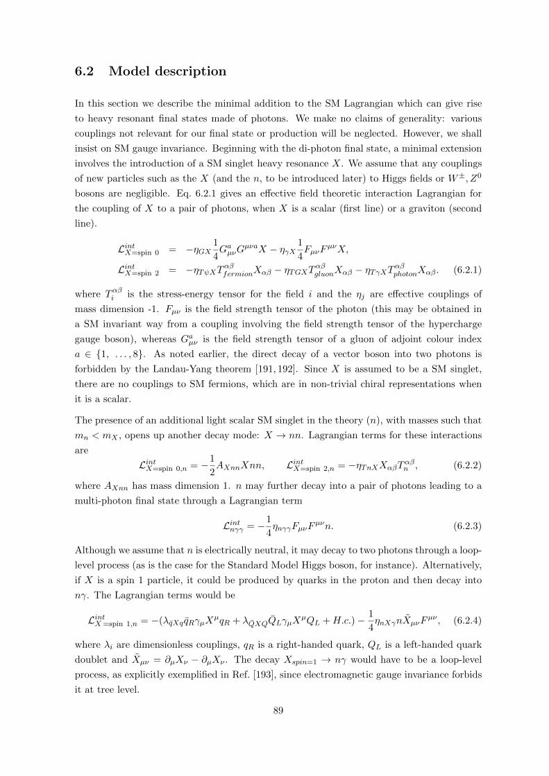
6.2 Model description
In this section we describe the minimal addition to the SM Lagrangian which can give rise
to heavy resonant final states made of photons. We make no claims of generality: various
couplings not relevant for our final state or production will be neglected. However, we shall
insist on SM gauge invariance. Beginning with the di-photon final state, a minimal extension
involves the introduction of a SM singlet heavy resonance X. We assume that any couplings
of new particles such as the X (and the n, to be introduced later) to Higgs fields or W±, Z0
bosons are negligible. Eq. 6.2.1 gives an effective field theoretic interaction Lagrangian for
the coupling of X to a pair of photons, when X is a scalar (first line) or a graviton (second
line).
LintX=spin 0 = −ηGX1
4GaµνG
µνaX − ηγX1
4FµνF
µνX,
LintX=spin 2 = −ηTψXTαβfermionXαβ − ηTGXTαβgluonXαβ − ηTγXTαβphotonXαβ. (6.2.1)
where Tαβi is the stress-energy tensor for the field i and the ηj are effective couplings of
mass dimension -1. Fµν is the field strength tensor of the photon (this may be obtained in
a SM invariant way from a coupling involving the field strength tensor of the hypercharge
gauge boson), whereas Gaµν is the field strength tensor of a gluon of adjoint colour index
a ∈ {1, . . . , 8}. As noted earlier, the direct decay of a vector boson into two photons is
forbidden by the Landau-Yang theorem [191, 192]. Since X is assumed to be a SM singlet,
there are no couplings to SM fermions, which are in non-trivial chiral representations when
it is a scalar.
The presence of an additional light scalar SM singlet in the theory (n), with masses such that
mn < mX , opens up another decay mode: X → nn. Lagrangian terms for these interactions
are
LintX=spin 0,n = −1
2AXnnXnn, LintX=spin 2,n = −ηTnXXαβT
αβn , (6.2.2)
where AXnn has mass dimension 1. n may further decay into a pair of photons leading to a
multi-photon final state through a Lagrangian term
Lintnγγ = −1
4ηnγγFµνF
µνn. (6.2.3)
Although we assume that n is electrically neutral, it may decay to two photons through a loop-
level process (as is the case for the Standard Model Higgs boson, for instance). Alternatively,
if X is a spin 1 particle, it could be produced by quarks in the proton and then decay into
nγ. The Lagrangian terms would be
LintX =spin 1,n = −(λqXq qRγµXµqR + λQXQQLγµX
µQL +H.c.)− 1
4ηnXγnXµνF
µν , (6.2.4)
where λi are dimensionless couplings, qR is a right-handed quark, QL is a left-handed quark
doublet and Xµν = ∂µXν − ∂µXν . The decay Xspin=1 → nγ would have to be a loop-level
process, as explicitly exemplified in Ref. [193], since electromagnetic gauge invariance forbids
it at tree level.
89
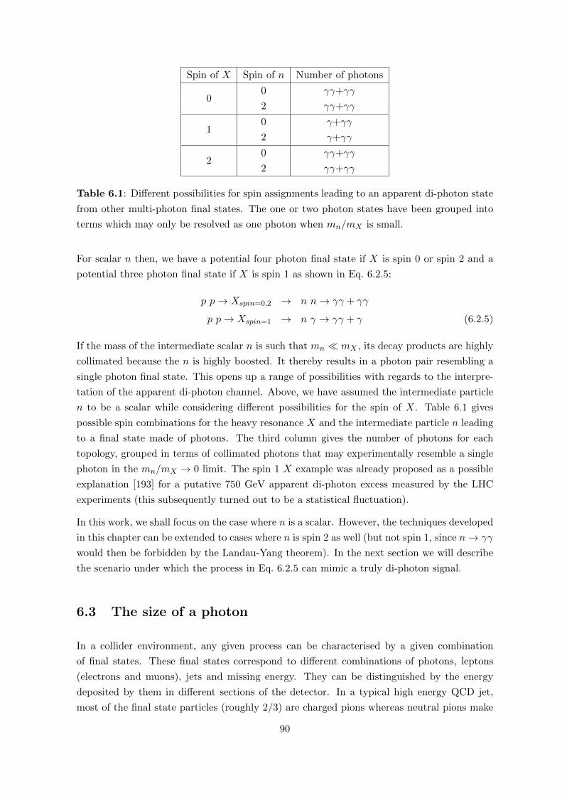
Spin of X Spin of n Number of photons
00 γγ+γγ
2 γγ+γγ
10 γ+γγ
2 γ+γγ
20 γγ+γγ
2 γγ+γγ
Table 6.1: Different possibilities for spin assignments leading to an apparent di-photon state
from other multi-photon final states. The one or two photon states have been grouped into
terms which may only be resolved as one photon when mn/mX is small.
For scalar n then, we have a potential four photon final state if X is spin 0 or spin 2 and a
potential three photon final state if X is spin 1 as shown in Eq. 6.2.5:
p p→ Xspin=0,2 → n n→ γγ + γγ
p p→ Xspin=1 → n γ → γγ + γ (6.2.5)
If the mass of the intermediate scalar n is such that mn � mX , its decay products are highly
collimated because the n is highly boosted. It thereby results in a photon pair resembling a
single photon final state. This opens up a range of possibilities with regards to the interpre-
tation of the apparent di-photon channel. Above, we have assumed the intermediate particle
n to be a scalar while considering different possibilities for the spin of X. Table 6.1 gives
possible spin combinations for the heavy resonance X and the intermediate particle n leading
to a final state made of photons. The third column gives the number of photons for each
topology, grouped in terms of collimated photons that may experimentally resemble a single
photon in the mn/mX → 0 limit. The spin 1 X example was already proposed as a possible
explanation [193] for a putative 750 GeV apparent di-photon excess measured by the LHC
experiments (this subsequently turned out to be a statistical fluctuation).
In this work, we shall focus on the case where n is a scalar. However, the techniques developed
in this chapter can be extended to cases where n is spin 2 as well (but not spin 1, since n→ γγ
would then be forbidden by the Landau-Yang theorem). In the next section we will describe
the scenario under which the process in Eq. 6.2.5 can mimic a truly di-photon signal.
6.3 The size of a photon
In a collider environment, any given process can be characterised by a given combination
of final states. These final states correspond to different combinations of photons, leptons
(electrons and muons), jets and missing energy. They can be distinguished by the energy
deposited by them in different sections of the detector. In a typical high energy QCD jet,
most of the final state particles (roughly 2/3) are charged pions whereas neutral pions make
90
up much of the remaining 1/3 [190]. The constituents of a jet primarily deposit their energy
in the hadronic calorimeter (HCAL) while the π0 → 2γ decay of a neutral pion ensures that it
shows up in the electromagnetic calorimeter (ECAL). Thus most of the constituents of the jet
pass through the ECAL and deposit their energy in the HCAL. Photons and electrons deposit
their energy in the ECAL, on the other hand. They can be distinguished by mapping the
energy deposition to the tracker (which precedes the calorimeters). Apart from the tracker,
electrons and photons are similar in appearance, from a detector point of view. Muons are
detected by the muon spectrometer on the outside of the experiment.
The experimental sensitivity to detect a single photon is subject to the following two criteria:
(a) Dimensions of the ECAL cells: The ATLAS and CMS detectors have slightly different
dimensions for the ECAL cells. ATLAS has a slightly coarser granularity with a crystal size
of (0.0256, 0.0254) in (η, φ). In comparison, CMS has a granularity of (0.0174, 0.0174) in
(η, φ). CMS and ATLAS have a pre-shower layer in the electromagnetic calorimeter with finer
η segmentation, which should also be employed in analyses looking for resonances into multi-
photon final states. The details of this layer are not available to us, and so we do not discuss it
further. However, we bear in mind that information from the pre-shower layer may be used in
addition to the techniques developed in this chapter. Any estimates of sensitivity (which come
later) are therefore conservative in the sense that additional information from the pre-shower
layer should improve the sensitivity. High energy photons will tend to shower in the ECAL:
this is taken into account by clustering the cells into cones of size Rcone = ∆R = 0.1. Thus
if two high energy signal photons are separated a distance ∆R < Rcone, they are typically
not considered to be resolved by the ECAL since it could be a single photon that is simply
showering.
(b) Photon isolation: In ATLAS and in CMS, a photon is considered to be isolated if
the magnitude of the vector sum of the transverse momenta (pT ) of all objects with ∆R ∈[Rcone, 0.4] is less than 10% of its pT . Qualitatively, this corresponds to the requirement
that most of the energy is carried by the photon around which the cone is constructed. This
criterion is required in order to distinguish a hard photon from a photon from a π0 decay.
However, it is possible that certain signal topologies may give rise final state photons that
are separated by a distance ∆R ∈ [Rcone, 0.4]. For instance, consider the process given in
Eq. 6.2.5. The particle X can either be a scalar or a graviton. For concreteness, let us assume
that n is a scalar. In this case, a four photon final state resulting from X → nn → γγ + γγ
would appear to be a di-photon final state. However, as mn increases, eventually ∆R > 0.4
and the number of resolved final state photons will increase. Similar arguments hold for the
case where particle X is a spin 1 state. For a given mass of n, the eventual number of detected,
isolated and resolved photons depends on the granularity of the detector and is expected to
be slightly different for both the CMS and ATLAS.
To approximate the acceptance and efficiency of the detectors for our signal process, we
perform a Monte-Carlo simulation using the following steps:
• The matrix element for our signal process is generated in MadGraph5 aMC@NLO [123]
91
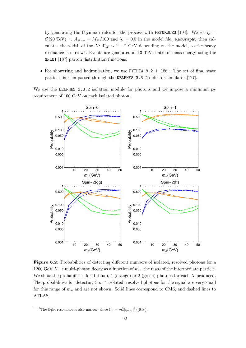
by generating the Feynman rules for the process with FEYNRULES [194]. We set ηi =
O(20 TeV)−1, AXnn = MX/100 and λi = 0.5 in the model file. MadGraph5 then cal-
culates the width of the X: ΓX ∼ 1 − 2 GeV depending on the model, so the heavy
resonance is narrow2. Events are generated at 13 TeV centre of mass energy using the
NNLO1 [187] parton distribution functions.
• For showering and hadronisation, we use PYTHIA 8.2.1 [186]. The set of final state
particles is then passed through the DELPHES 3.3.2 detector simulator [127].
We use the DELPHES 3.3.2 isolation module for photons and we impose a minimum pT
requirement of 100 GeV on each isolated photon.
10 20 30 40 500.001
0.005
0.010
0.050
0.100
0.500
1
mn(GeV)
Probability
Spin-0
10 20 30 40 500.001
0.005
0.010
0.050
0.100
0.500
1
mn(GeV)
Probability
Spin-1
10 20 30 40 500.001
0.005
0.010
0.050
0.100
0.500
1
mn(GeV)
Probability
Spin-2(gg)
10 20 30 40 500.001
0.005
0.010
0.050
0.100
0.500
1
mn(GeV)
Probability
Spin-2(ff)
Figure 6.2: Probabilities of detecting different numbers of isolated, resolved photons for a
1200 GeV X → multi-photon decay as a function of mn, the mass of the intermediate particle.
We show the probabilities for 0 (blue), 1 (orange) or 2 (green) photons for each X produced.
The probabilities for detecting 3 or 4 isolated, resolved photons for the signal are very small
for this range of mn and are not shown. Solid lines correspond to CMS, and dashed lines to
ATLAS.
2The light resonance is also narrow, since Γn = m3n|ηnγγ |2/(64π).
92
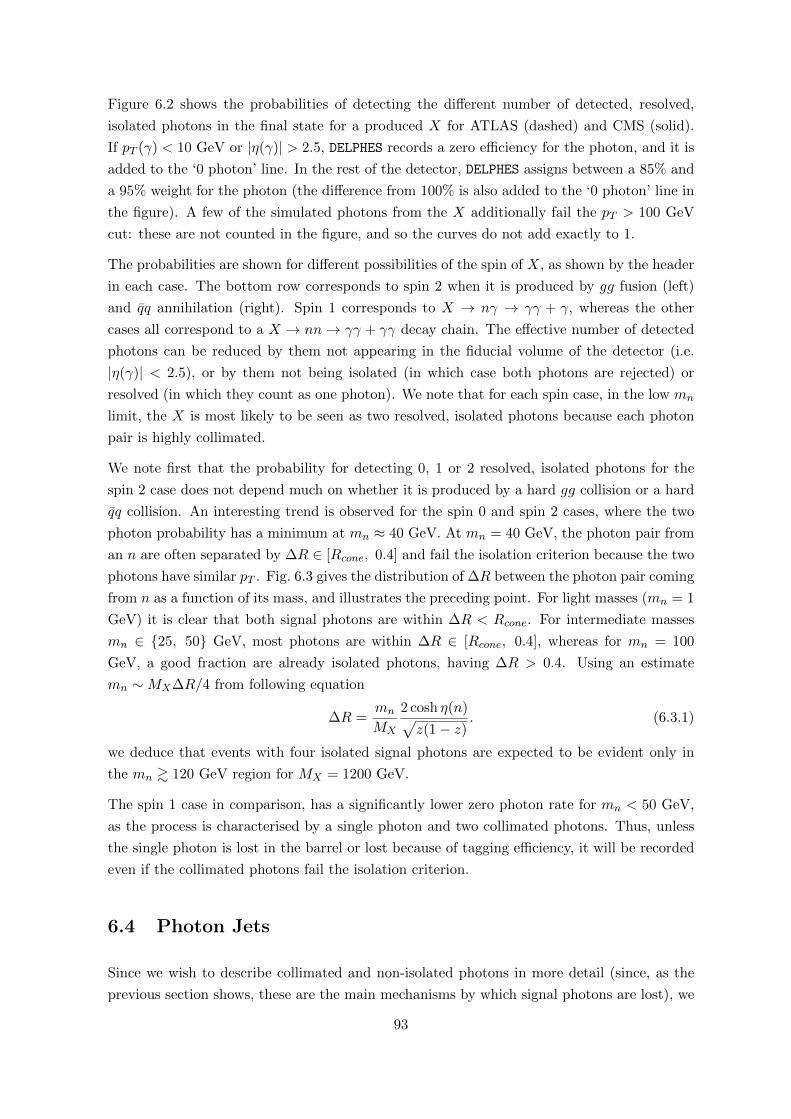
Figure 6.2 shows the probabilities of detecting the different number of detected, resolved,
isolated photons in the final state for a produced X for ATLAS (dashed) and CMS (solid).
If pT (γ) < 10 GeV or |η(γ)| > 2.5, DELPHES records a zero efficiency for the photon, and it is
added to the ‘0 photon’ line. In the rest of the detector, DELPHES assigns between a 85% and
a 95% weight for the photon (the difference from 100% is also added to the ‘0 photon’ line in
the figure). A few of the simulated photons from the X additionally fail the pT > 100 GeV
cut: these are not counted in the figure, and so the curves do not add exactly to 1.
The probabilities are shown for different possibilities of the spin of X, as shown by the header
in each case. The bottom row corresponds to spin 2 when it is produced by gg fusion (left)
and qq annihilation (right). Spin 1 corresponds to X → nγ → γγ + γ, whereas the other
cases all correspond to a X → nn→ γγ + γγ decay chain. The effective number of detected
photons can be reduced by them not appearing in the fiducial volume of the detector (i.e.
|η(γ)| < 2.5), or by them not being isolated (in which case both photons are rejected) or
resolved (in which they count as one photon). We note that for each spin case, in the low mn
limit, the X is most likely to be seen as two resolved, isolated photons because each photon
pair is highly collimated.
We note first that the probability for detecting 0, 1 or 2 resolved, isolated photons for the
spin 2 case does not depend much on whether it is produced by a hard gg collision or a hard
qq collision. An interesting trend is observed for the spin 0 and spin 2 cases, where the two
photon probability has a minimum at mn ≈ 40 GeV. At mn = 40 GeV, the photon pair from
an n are often separated by ∆R ∈ [Rcone, 0.4] and fail the isolation criterion because the two
photons have similar pT . Fig. 6.3 gives the distribution of ∆R between the photon pair coming
from n as a function of its mass, and illustrates the preceding point. For light masses (mn = 1
GeV) it is clear that both signal photons are within ∆R < Rcone. For intermediate masses
mn ∈ {25, 50} GeV, most photons are within ∆R ∈ [Rcone, 0.4], whereas for mn = 100
GeV, a good fraction are already isolated photons, having ∆R > 0.4. Using an estimate
mn ∼MX∆R/4 from following equation
∆R =mn
MX
2 cosh η(n)√z(1− z)
. (6.3.1)
we deduce that events with four isolated signal photons are expected to be evident only in
the mn & 120 GeV region for MX = 1200 GeV.
The spin 1 case in comparison, has a significantly lower zero photon rate for mn < 50 GeV,
as the process is characterised by a single photon and two collimated photons. Thus, unless
the single photon is lost in the barrel or lost because of tagging efficiency, it will be recorded
even if the collimated photons fail the isolation criterion.
6.4 Photon Jets
Since we wish to describe collimated and non-isolated photons in more detail (since, as the
previous section shows, these are the main mechanisms by which signal photons are lost), we
93
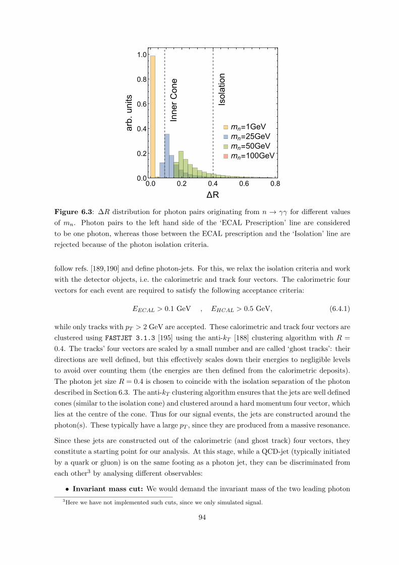
mn=1GeV
mn=25GeV
mn=50GeV
mn=100GeV
Inn
er
Co
ne
Iso
latio
n
0.0 0.2 0.4 0.6 0.80.0
0.2
0.4
0.6
0.8
1.0
ΔR
arb
.u
nits
Figure 6.3: ∆R distribution for photon pairs originating from n → γγ for different values
of mn. Photon pairs to the left hand side of the ‘ECAL Prescription’ line are considered
to be one photon, whereas those between the ECAL prescription and the ‘Isolation’ line are
rejected because of the photon isolation criteria.
follow refs. [189,190] and define photon-jets. For this, we relax the isolation criteria and work
with the detector objects, i.e. the calorimetric and track four vectors. The calorimetric four
vectors for each event are required to satisfy the following acceptance criteria:
EECAL > 0.1 GeV , EHCAL > 0.5 GeV, (6.4.1)
while only tracks with pT > 2 GeV are accepted. These calorimetric and track four vectors are
clustered using FASTJET 3.1.3 [195] using the anti-kT [188] clustering algorithm with R =
0.4. The tracks’ four vectors are scaled by a small number and are called ‘ghost tracks’: their
directions are well defined, but this effectively scales down their energies to negligible levels
to avoid over counting them (the energies are then defined from the calorimetric deposits).
The photon jet size R = 0.4 is chosen to coincide with the isolation separation of the photon
described in Section 6.3. The anti-kT clustering algorithm ensures that the jets are well defined
cones (similar to the isolation cone) and clustered around a hard momentum four vector, which
lies at the centre of the cone. Thus for our signal events, the jets are constructed around the
photon(s). These typically have a large pT , since they are produced from a massive resonance.
Since these jets are constructed out of the calorimetric (and ghost track) four vectors, they
constitute a starting point for our analysis. At this stage, while a QCD-jet (typically initiated
by a quark or gluon) is on the same footing as a photon jet, they can be discriminated from
each other3 by analysing different observables:
• Invariant mass cut: We would demand the invariant mass of the two leading photon
3Here we have not implemented such cuts, since we only simulated signal.
94
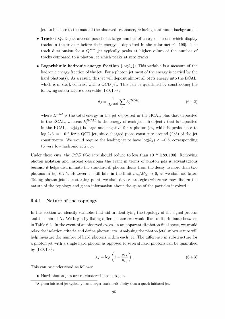
jets to be close to the mass of the observed resonance, reducing continuum backgrounds.
• Tracks: QCD jets are composed of a large number of charged mesons which display
tracks in the tracker before their energy is deposited in the calorimeter4 [196]. The
track distribution for a QCD jet typically peaks at higher values of the number of
tracks compared to a photon jet which peaks at zero tracks.
• Logarithmic hadronic energy fraction (log θJ): This variable is a measure of the
hadronic energy fraction of the jet. For a photon jet most of the energy is carried by the
hard photon(s). As a result, this jet will deposit almost all of its energy into the ECAL,
which is in stark contrast with a QCD jet. This can be quantified by constructing the
following substructure observable [189,190]:
θJ =1
Etotal
∑i
EHCALi , (6.4.2)
where Etotal is the total energy in the jet deposited in the HCAL plus that deposited
in the ECAL, whereas EHCALi is the energy of each jet sub-object i that is deposited
in the HCAL. log(θJ) is large and negative for a photon jet, while it peaks close to
log[2/3] = −0.2 for a QCD jet, since charged pions constitute around (2/3) of the jet
constituents. We would require the leading jet to have log(θJ) < −0.5, corresponding
to very low hadronic activity.
Under these cuts, the QCD fake rate should reduce to less than 10−5 [189, 190]. Removing
photon isolation and instead describing the event in terms of photon jets is advantageous
because it helps discriminate the standard di-photon decay from the decay to more than two
photons in Eq. 6.2.5. However, it still fails in the limit mn/MX → 0, as we shall see later.
Taking photon jets as a starting point, we shall devise strategies where we may discern the
nature of the topology and glean information about the spins of the particles involved.
6.4.1 Nature of the topology
In this section we identify variables that aid in identifying the topology of the signal process
and the spin of X. We begin by listing different cases we would like to discriminate between
in Table 6.2. In the event of an observed excess in an apparent di-photon final state, we would
relax the isolation criteria and define photon jets. Analysing the photon jets’ substructure will
help measure the number of hard photons within each jet. The difference in substructure for
a photon jet with a single hard photon as opposed to several hard photons can be quantified
by [189,190]:
λJ = log
(1− pTL
pTJ
). (6.4.3)
This can be understood as follows:
• Hard photon jets are re-clustered into sub-jets.
4A gluon initiated jet typically has a larger track multiplicity than a quark initiated jet.
95
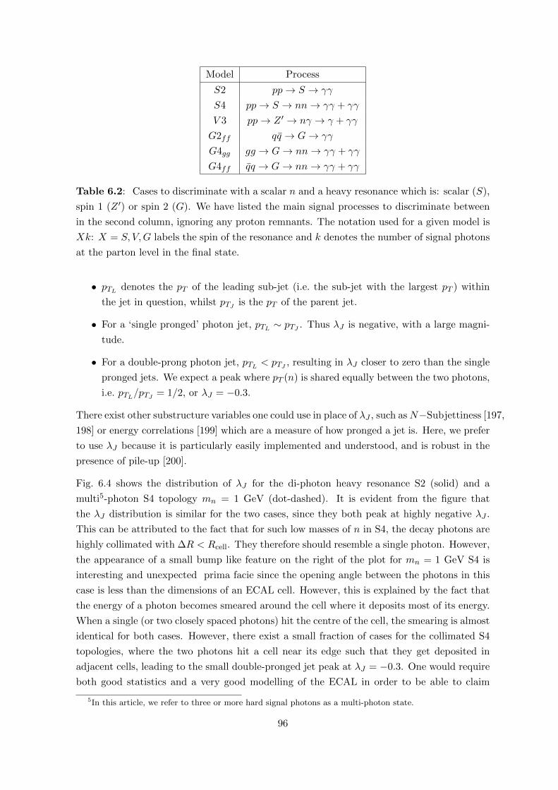
Model Process
S2 pp→ S → γγ
S4 pp→ S → nn→ γγ + γγ
V 3 pp→ Z ′ → nγ → γ + γγ
G2ff qq → G→ γγ
G4gg gg → G→ nn→ γγ + γγ
G4ff qq → G→ nn→ γγ + γγ
Table 6.2: Cases to discriminate with a scalar n and a heavy resonance which is: scalar (S),
spin 1 (Z ′) or spin 2 (G). We have listed the main signal processes to discriminate between
in the second column, ignoring any proton remnants. The notation used for a given model is
Xk: X = S, V,G labels the spin of the resonance and k denotes the number of signal photons
at the parton level in the final state.
• pTL denotes the pT of the leading sub-jet (i.e. the sub-jet with the largest pT ) within
the jet in question, whilst pTJ is the pT of the parent jet.
• For a ‘single pronged’ photon jet, pTL ∼ pTJ . Thus λJ is negative, with a large magni-
tude.
• For a double-prong photon jet, pTL < pTJ , resulting in λJ closer to zero than the single
pronged jets. We expect a peak where pT (n) is shared equally between the two photons,
i.e. pTL/pTJ = 1/2, or λJ = −0.3.
There exist other substructure variables one could use in place of λJ , such asN−Subjettiness [197,
198] or energy correlations [199] which are a measure of how pronged a jet is. Here, we prefer
to use λJ because it is particularly easily implemented and understood, and is robust in the
presence of pile-up [200].
Fig. 6.4 shows the distribution of λJ for the di-photon heavy resonance S2 (solid) and a
multi5-photon S4 topology mn = 1 GeV (dot-dashed). It is evident from the figure that
the λJ distribution is similar for the two cases, since they both peak at highly negative λJ .
This can be attributed to the fact that for such low masses of n in S4, the decay photons are
highly collimated with ∆R < Rcell. They therefore should resemble a single photon. However,
the appearance of a small bump like feature on the right of the plot for mn = 1 GeV S4 is
interesting and unexpected prima facie since the opening angle between the photons in this
case is less than the dimensions of an ECAL cell. However, this is explained by the fact that
the energy of a photon becomes smeared around the cell where it deposits most of its energy.
When a single (or two closely spaced photons) hit the centre of the cell, the smearing is almost
identical for both cases. However, there exist a small fraction of cases for the collimated S4
topologies, where the two photons hit a cell near its edge such that they get deposited in
adjacent cells, leading to the small double-pronged jet peak at λJ = −0.3. One would require
both good statistics and a very good modelling of the ECAL in order to be able to claim
5In this article, we refer to three or more hard signal photons as a multi-photon state.
96
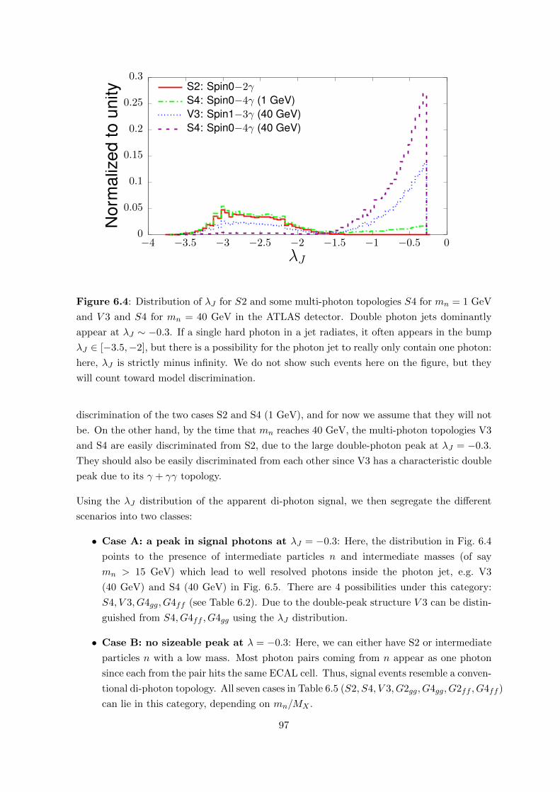
0
0.05
0.1
0.15
0.2
0.25
0.3
−4 −3.5 −3 −2.5 −2 −1.5 −1 −0.5 0
Nor
mal
ized
toun
ity
λJ
S2: Spin0−2γ
S4: Spin0−4γ (1 GeV)V3: Spin1−3γ (40 GeV)S4: Spin0−4γ (40 GeV)
Figure 6.4: Distribution of λJ for S2 and some multi-photon topologies S4 for mn = 1 GeV
and V 3 and S4 for mn = 40 GeV in the ATLAS detector. Double photon jets dominantly
appear at λJ ∼ −0.3. If a single hard photon in a jet radiates, it often appears in the bump
λJ ∈ [−3.5,−2], but there is a possibility for the photon jet to really only contain one photon:
here, λJ is strictly minus infinity. We do not show such events here on the figure, but they
will count toward model discrimination.
discrimination of the two cases S2 and S4 (1 GeV), and for now we assume that they will not
be. On the other hand, by the time that mn reaches 40 GeV, the multi-photon topologies V3
and S4 are easily discriminated from S2, due to the large double-photon peak at λJ = −0.3.
They should also be easily discriminated from each other since V3 has a characteristic double
peak due to its γ + γγ topology.
Using the λJ distribution of the apparent di-photon signal, we then segregate the different
scenarios into two classes:
• Case A: a peak in signal photons at λJ = −0.3: Here, the distribution in Fig. 6.4
points to the presence of intermediate particles n and intermediate masses (of say
mn > 15 GeV) which lead to well resolved photons inside the photon jet, e.g. V3
(40 GeV) and S4 (40 GeV) in Fig. 6.5. There are 4 possibilities under this category:
S4, V 3, G4gg, G4ff (see Table 6.2). Due to the double-peak structure V 3 can be distin-
guished from S4, G4ff , G4gg using the λJ distribution.
• Case B: no sizeable peak at λ = −0.3: Here, we can either have S2 or intermediate
particles n with a low mass. Most photon pairs coming from n appear as one photon
since each from the pair hits the same ECAL cell. Thus, signal events resemble a conven-
tional di-photon topology. All seven cases in Table 6.5 (S2, S4, V 3, G2gg, G4gg, G2ff , G4ff )
can lie in this category, depending on mn/MX .
97
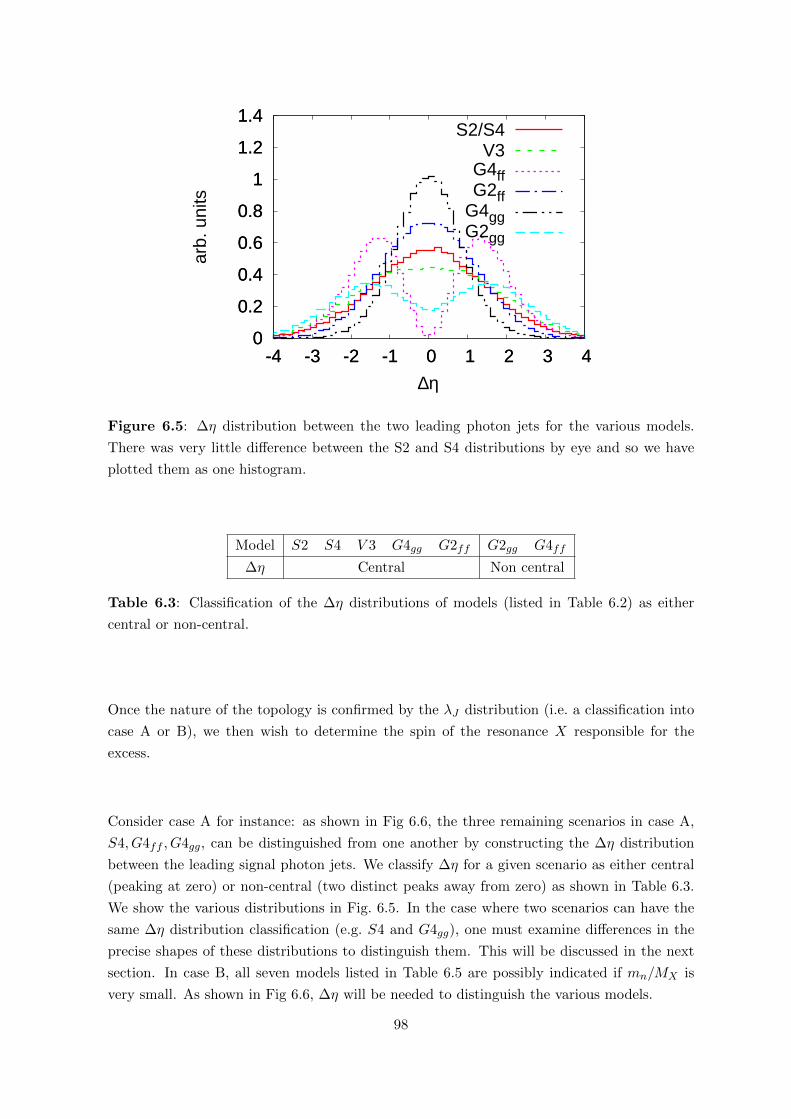
0
0.2
0.4
0.6
0.8
1
1.2
1.4
-4 -3 -2 -1 0 1 2 3 4
arb.
uni
ts
∆η
S2/S4V3
G4ffG2ff
G4ggG2gg
0
0.2
0.4
0.6
0.8
1
1.2
1.4
-4 -3 -2 -1 0 1 2 3 4
Figure 6.5: ∆η distribution between the two leading photon jets for the various models.
There was very little difference between the S2 and S4 distributions by eye and so we have
plotted them as one histogram.
Model S2 S4 V 3 G4gg G2ff G2gg G4ff
∆η Central Non central
Table 6.3: Classification of the ∆η distributions of models (listed in Table 6.2) as either
central or non-central.
Once the nature of the topology is confirmed by the λJ distribution (i.e. a classification into
case A or B), we then wish to determine the spin of the resonance X responsible for the
excess.
Consider case A for instance: as shown in Fig 6.6, the three remaining scenarios in case A,
S4, G4ff , G4gg, can be distinguished from one another by constructing the ∆η distribution
between the leading signal photon jets. We classify ∆η for a given scenario as either central
(peaking at zero) or non-central (two distinct peaks away from zero) as shown in Table 6.3.
We show the various distributions in Fig. 6.5. In the case where two scenarios can have the
same ∆η distribution classification (e.g. S4 and G4gg), one must examine differences in the
precise shapes of these distributions to distinguish them. This will be discussed in the next
section. In case B, all seven models listed in Table 6.5 are possibly indicated if mn/MX is
very small. As shown in Fig 6.6, ∆η will be needed to distinguish the various models.
98
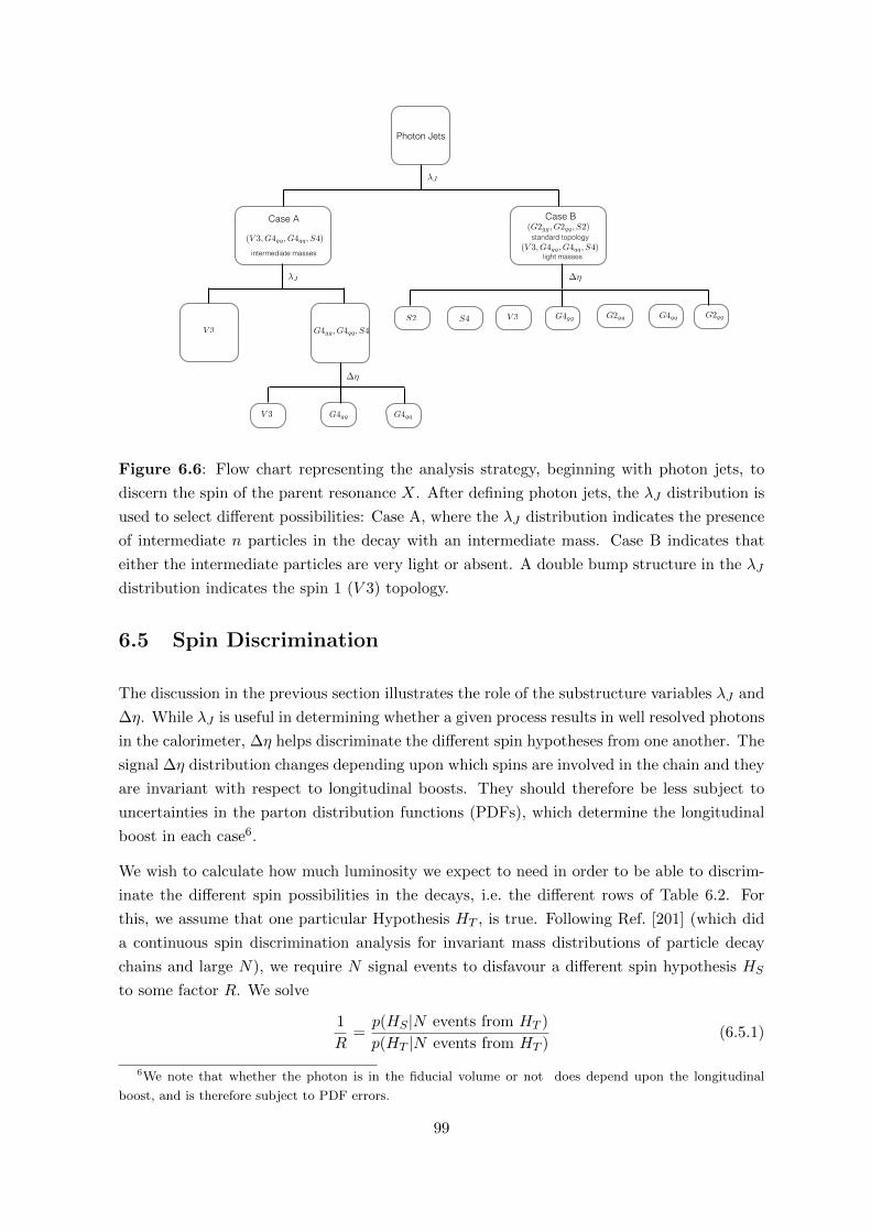
Photon Jets
G4gg, G4qq, S4V 3
(V 3, G4gg, G4qq, S4)
Case A
(V 3, G4gg, G4qq, S4)
Case B(G2gg, G2qq, S2)
S2 S4 V 3 G4gg G2gg G4qq G2qq
G4gg G4qqV 3
�J
�J �⌘
�⌘
intermediate masses light masses
standard topology
Figure 6.6: Flow chart representing the analysis strategy, beginning with photon jets, to
discern the spin of the parent resonance X. After defining photon jets, the λJ distribution is
used to select different possibilities: Case A, where the λJ distribution indicates the presence
of intermediate n particles in the decay with an intermediate mass. Case B indicates that
either the intermediate particles are very light or absent. A double bump structure in the λJ
distribution indicates the spin 1 (V 3) topology.
6.5 Spin Discrimination
The discussion in the previous section illustrates the role of the substructure variables λJ and
∆η. While λJ is useful in determining whether a given process results in well resolved photons
in the calorimeter, ∆η helps discriminate the different spin hypotheses from one another. The
signal ∆η distribution changes depending upon which spins are involved in the chain and they
are invariant with respect to longitudinal boosts. They should therefore be less subject to
uncertainties in the parton distribution functions (PDFs), which determine the longitudinal
boost in each case6.
We wish to calculate how much luminosity we expect to need in order to be able to discrim-
inate the different spin possibilities in the decays, i.e. the different rows of Table 6.2. For
this, we assume that one particular Hypothesis HT , is true. Following Ref. [201] (which did
a continuous spin discrimination analysis for invariant mass distributions of particle decay
chains and large N), we require N signal events to disfavour a different spin hypothesis HS
to some factor R. We solve
1
R=p(HS |N events from HT )
p(HT |N events from HT )(6.5.1)
6We note that whether the photon is in the fiducial volume or not does depend upon the longitudinal
boost, and is therefore subject to PDF errors.
99
for N , for some given R (here we will require R = 20, i.e. that some spin hypothesis HS
is disfavoured at 20:1 odds over another HT ). We are explicitly assuming that background
contributions B are negligible to make our estimate, but in practice, they could be included
in the ∆η distributions in which case HS → HS +B and HT → HT +B in Eq. 6.5.1.
We characterise the ‘N events from HT ’ by the values of a particular observable (or set of
observables) oi. In the present chapter, we shall consider the pseudrapidity difference ∆η
between the leading and next-to-leading photon jet, o(T )i (for i ∈ {1, 2, . . . , N}) that are
observed in those events, although the observables could easily be extended to include other
observables, for example λJ . By Bayes’ Theorem, we rewrite Eq. 6.5.1 as
1
R=p(HS)
p(HT )
p(N events from HT |HS)
p(N events from HT |HT )=p(HS)
p(HT )
∏Ni=1 p(o
(T )i |HS)∏N
i=1 p(o(T )i |HT )
. (6.5.2)
Binned data measured in the o distribution {n(T )j } (for j ∈ {1, 2, . . . ,K}, K being the number
of bins), will be Poisson distributed7 based on the expectation µ(X)j for bin j:
p(nj |HX) = Pois(nj |µ(X)j ), (6.5.3)
where X ∈ {S, T} and Pois(n|µ) = µne−µ
n! . Substituting this into Eq. 6.5.2, we obtain
log
(1
R
)= log
(p(HS)
p(HT )
)+
K∑j=1
[n
(T )j log
µ(S)j
µ(T )j
+ µ(T )j − µ(S)
j
], (6.5.4)
where µ(T )j is the expectation of the number of events in bin j from HT and n
(T )j is a random
sample of observed events obtained from p(nj |HT ). There is a (hopefully small) amount of
information lost in going between unbinned data in Eq. 6.5.2 and binned data in Eq. 6.5.4.
The first term on the right hand side contains the ratio of prior probabilities of HT and
HS : this ratio we will set to one, having no particular a priori preference. Then taking the
expectation over many draws, 〈n(T )j 〉 = µ
(T )j and so
log
(1
R
)=
K∑i=1
[µ
(T )j log
µ(S)j
µ(T )j
+ µ(T )j − µ(S)
j
]. (6.5.5)
We notice that Eq. 6.5.5 is not antisymmetric under T ↔ S, but this is expected since we
are assuming that HT is the true hypothesis, in contrast to HS . As the data come in, at
some integrated luminosity, the distribution will be sufficiently different from the prediction
of some other hypothesis, HS , to discriminate against it at the level of 20 times as likely.
Each term on the right-hand side is proportional to the integrated luminosity collected L,
µ(X)j = Lσ(X)
tot ε(X)j , (6.5.6)
7As argued above, we work in kinematic regimes where backgrounds can be neglected. We are also neglecting
theoretical errors in our signal predictions. It would be straightforward to extend our analysis to the case where
some smearing due to theoretical uncertainties is included, where we would convolute Eq. 6.5.3 with a Gaussian
distribution.
100
where σ(X)tot is the assumed total signal cross-section (i.e. the X production cross section)
before cuts for HX and ε(X)j is the probability that a signal event makes it past all of the
cuts and into bin j, under hypothesis X. Assuming that σStot = σTtot ≡ σtot, we may solve
Eq. 6.5.5 and Eq. 6.5.6 for NR = Lσtot, the expected number of total signal events required
to disfavour HS over HT to an odds factor of R:
NR =logR∑K
j=1
[ε(T )j log
ε(T )j
ε(S)j
+ ε(S)j − ε(T )
j
] . (6.5.7)
One property of this equation is that if ε(T )j = ε
(S)j ∀ j, then LR →∞. This makes sense: there
is no luminosity large enough such that it can discriminate between identical distributions.
Eq. 6.5.7 works for multi-dimensional cases of several observables: one simply gets more bins
for the multi-dimensional case. If one works in the large statistics limit, for continuous data
(rather than binned data), one obtains a required number of events that is related [201] to the
Kullback-Leibler divergence instead [202]. The Kullback-Leibler divergence is commonly used
when one has analytic expressions for distributions of the observables (see Ref. [201]), and has
the advantage of utilizing the full information in o. We do not have analytic expressions, partly
because they depend upon parton distribution functions, which are numerically calculated.
Our method loses some information by binning, but it has the considerable advantage that
it includes kinematical selection and detector effects (all contained within the εj). Eq. 6.5.7
has the property that: if one halves the total X production cross-section, one requires double
the luminosity to keep the discrimination power (measured by R) constant.
Since we shall estimate ε(X)j numerically via Monte-Carlo event generation, there is a potential
problem we have to deal with: a bin might end up with no generated events and so one
encounters divergences from the logarithm in the denominator of Eq. 6.5.7. This is due,
however, to not using enough Monte Carlo statistics, where M signal events are simulated in
total for each parameter choice and for each hypothesis pairing. We restrict the range of o
and use large enough Monte Carlo statistics (M = 200000) such that no bins (that are set to
be wide enough) contain zero events.
6.5.1 Event Selection and Results
Using the statistic developed in Eq. 6.5.7, we first first discriminate Case A from B defined in
Section 6.4.1. Thus, in the event of an apparent di-photon excess in a certain invariant mass
bin say m(0)γγ , we propose the following steps:
• We relax the isolation criteria and re-analyse the events by constructing photon jets.
• The invariant mass mj1j2 of the two leading photon jets for each events are required to
lie around m(0)γγ : we require 1100 < mj1j2/GeV < 1300.
• Photon jets from pions are eliminated by requiring that leading jet to have no tracks
(nT = 0) and by requiring log θJ < −0.5. We also take into account the photon
101
conversion factor. This depends on whether the photon converts before or after exiting
the pixel detector. This conversion probability is a function of the number of radiation
lengths (a) a photon passes through before it escapes the first pixel detector and is given
by [190]
P (η) = 1− exp(−7
9a(η)). (6.5.8)
We approximate this by an η independent conversion probability P (η) = 0.2.
• The substructure of each jet is analysed using λJ to determine whether it is in Case A
or B.
Fig.6.6 gives a pictorial representation of these steps. We use mn = 40 GeV and mn = 1
GeV as examples for the model hypotheses to be tested. We simulate 2× 10⁵ events for the
topologies predicted by HT and HS and compute λJ for the all events which pass the basic
selection criteria. To avoid any zero event bins, λJ is binned between [−4, 0] with a bin size
of 0.6 and the efficiency for each particular bin is extracted for both distributions from the
simulation. Owing to the distinct nature of the λJ distribution for both the cases, 3-4 events
is sufficient to discriminate between case A and case B. The mn = 1, 40 GeV cases both have a
post-cut acceptance efficiency of ∼ 55%. For a cross-section of 0.5 fb, we can accumulate some
five signal events with ∼18 fb−1 of integrated luminosity. Once the nature of the topology
(corresponding to a given case) is identified, our next step is to discriminate the different
possibilities within it. Both of the scenarios are handled independently as follows:
CASE A: In this case there are only four possibilities corresponding to a multi-photon
topology (i.e. proceeding through an intermediate n). As discussed earlier, we do not impose
the requirement of two isolated photons, since the photons from n tend to fail isolation cuts.
We compute ∆η between the two leading photon jets. In order to discriminate V3 from the
other cases, the twin-peaked structure of V 3 under λJ (as shown in Fig 6.4.3) can be employed
to discriminate it collectively from S4, G4gg, G4ff . In this case one requires a minimum of
20 signal events to disfavour the other three at a 20 : 1 odds. All samples are characterised
by a minimum of ∼ 55% acceptance efficiency. With this information then, one can disfavour
S4, G4gg, G4ff in favour of V 3 with ∼ 72 fb−1 of integrated luminosity for a 0.5 fb signal
cross-section.
S4, G4gg, G4ff can then be discriminated from one another using ∆η between the two leading
jets. Table 6.4 computes the minimum number events required for pairwise discrimination of
the three cases for mn = 40 GeV and is computed using Eq. 6.5.7 To avoid zero event bins in
the ∆η distribution, we restrict the a priori range of |∆η| ∈ [−5, 5] to [−4, 4]. As shown in
the Table 6.4, disfavouring S4 as compared to G4gg constitutes the largest expected number
of required signal events i.e. 29. This can be achieved with a luminosity of ∼ 105 fb−1. Thus
in the event of a discovery corresponding to Case A, it is possible to get exact nature of the
spin of X within 105 fb−1 of data.
CASE B: This constitutes the more complicated of the two cases. Since the two hard photons
inside the photon-jet for the multi-photon topologies can not be well resolved, the substructure
is similar to the conventional single photon jet from the standard di-photon topology. Thus
102
NR S4 G4gg G4ff
S4 ∞ 22 13
G4gg 29 ∞ 4
G4ff 19 5 ∞
Table 6.4: Spin discrimination: NR = Lσ(X)tot , the expected number of total signal events
required to be produced to discriminate against the ‘true’ row model versus a column model
by a factor of 20 at the 13 TeV LHC for mn = 40 GeV.
there are more cases to distinguished in this case. We compute the ∆η between the leading
two jets of the event. To avoid zero event bins in the ∆η distribution, we restrict the a priori
range of ∆η from [−5, 5] to [−4, 4].
The signal models here are characterised by an acceptance efficiency of at least 55%. Using
the cross-section of 0.5 fb, we find that the cases S2 and S4 are virtually indistinguishable
owing to the similar shapes of their ∆η distributions. They thus cannot be distinguished on
the basis of the ∆η distribution. However, as shown in Fig. 6.4, the presence of secondary
bump for the collimated case will help in distinguishing these two cases. In this case, the
same technology we have developed for the ∆η distribution could be employed for the λJ
distribution.
Distinguishing S2, S4 from V 3 requires a maximum expected number of events of 250-300.
This is achievable with 1.1 ab−1 of integrated luminosity, assuming an acceptance of ∼ 55 %
and a signal production cross-section of 0.5 fb. Distinguishing scenarios like S2 from G4ff or
G4gg requires 23 events or less: these could be discriminated with ∼84 fb−1 for our reference
cross-section of 0.5 fb, whereas the rest of the pairs of spin hypotheses can be distinguished
within 364 fb−1 of data.
NR S2 S4 V 3 G2gg G4gg G2ff G4ff
S2 ∞ > 2000 272 27 15 91 14
S4 > 2000 ∞ 255 26 15 96 13
V 3 260 248 ∞ 54 9 37 21
G2gg 32 31 65 ∞ 5 13 38
G4gg 23 24 14 6 ∞ 54 4
G2ff 102 110 44 12 40 ∞ 8
G4ff 19 18 28 37 5 12 ∞
Table 6.5: Spin discrimination of two models: NR = Lσ(X)tot , the expected number of total
signal events required to be produced to discriminate against the ‘true’ row model versus a
column model by a factor of 20 at the 13 TeV LHC for mn = 1 GeV.
103
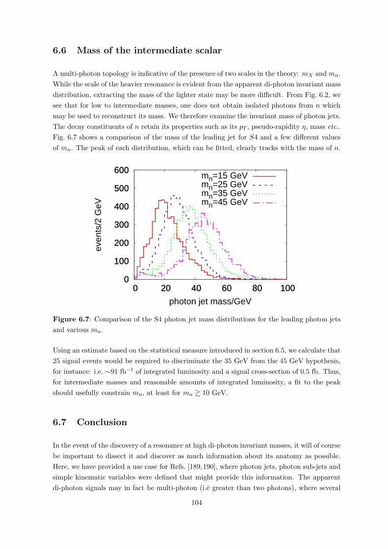
6.6 Mass of the intermediate scalar
A multi-photon topology is indicative of the presence of two scales in the theory: mX and mn.
While the scale of the heavier resonance is evident from the apparent di-photon invariant mass
distribution, extracting the mass of the lighter state may be more difficult. From Fig. 6.2, we
see that for low to intermediate masses, one does not obtain isolated photons from n which
may be used to reconstruct its mass. We therefore examine the invariant mass of photon jets.
The decay constituents of n retain its properties such as its pT , pseudo-rapidity η, mass etc..
Fig. 6.7 shows a comparison of the mass of the leading jet for S4 and a few different values
of mn. The peak of each distribution, which can be fitted, clearly tracks with the mass of n.
0
100
200
300
400
500
600
0 20 40 60 80 100
even
ts/2
GeV
photon jet mass/GeV
mn=15 GeVmn=25 GeVmn=35 GeVmn=45 GeV
0
100
200
300
400
500
600
0 20 40 60 80 100
Figure 6.7: Comparison of the S4 photon jet mass distributions for the leading photon jets
and various mn.
Using an estimate based on the statistical measure introduced in section 6.5, we calculate that
25 signal events would be required to discriminate the 35 GeV from the 45 GeV hypothesis,
for instance: i.e. ∼91 fb−1 of integrated luminosity and a signal cross-section of 0.5 fb. Thus,
for intermediate masses and reasonable amounts of integrated luminosity, a fit to the peak
should usefully constrain mn, at least for mn & 10 GeV.
6.7 Conclusion
In the event of the discovery of a resonance at high di-photon invariant masses, it will of course
be important to dissect it and discover as much information about its anatomy as possible.
Here, we have provided a use case for Refs. [189,190], where photon jets, photon sub-jets and
simple kinematic variables were defined that might provide this information. The apparent
di-photon signals may in fact be multi-photon (i.e greater than two photons), where several
104

photons are collinear, as is expected when intermediate particles have a mass much less than
the mass of the original resonance. We identified useful variables for this purpose: the pseudo-
rapidity difference between the photon jets helps discriminate different spin combinations of
the two new particles in the decays. We quantify an estimate for how many signal events are
expected to be required to provide discrimination between different spin hypotheses, setting
up a discrete version of the Kullback-Leibler divergence for the purpose. For the discovery of
a 1200 GeV resonance with a signal cross-section of 05 fb, many of the spin possibilities can be
discriminated within the expected total integrated luminosity expected to be obtained from
the LHC. A simple sub-jet variable λJ provides a good discriminant between the di-photon
and multi-photon cases. The invariant mass of the individual photon jets provides useful
information about the intermediate resonance mass.
105
Chapter 7
Summary and concluding remarks
The present searches at the Large Hadron Collider have witnessed no success in determining
any signs of new physics apart from few glitches in the charged and neutral B meson decays.
With more and more statistics, the SM seems to be emerging as the sole winner. Since the
race is not yet over, however, we cannot be sure of its outcome. There is still much room for
new physics and it is in this context that we have studied four different new physics scenarios.
These scenarios have mostly dealt with the determination of direct and indirect hints of new
bosonic physics1 at the Large Hadron Collider.
Probes of new physics depend on the scales at which observable effects emerge. While lighter
particles could be probed as resonances at the colliders, the heavier particles rely on the
indirect hints where for instance a well-measured observable significantly differs from its SM
prediction. Note that the definition of lighter and heavier is relative and depends on the
center of mass energy probed by a particular collider.
Given the lack of experimental evidences and with well-motivated models failing to show their
mark at the collider, the strategy followed in the thesis has been primarily to understand the
fluctuations in the data and eventually make predictions by either constructing or considering
simple extensions of SM in a bottom-up approach. The advantage of this approach is that
it is mostly unbiased and could help to point towards the full UV-complete theory in future.
Till then our job is essentially to collect the missing pieces of the puzzle.
A wide range of analyses have been performed using these techniques ranging from deter-
mining class of U(1)X models to explain the hints of lepton flavour universality violation
in neutral B-decays to finding signs of new physics in diphoton resonances to probing the
well-measured gauge boson vertices. In performing these analyses, a number of ”clean” final
states have been analyzed ranging from γγ to di-muons to Wγ, where leptonic decays of W
are considered, for different NP scenarios. The interesting regions/channels which could be
probed at the recent runs of the LHC have been identified Luminosity. Now it remains to be
1The choice of bosonic signals is partly motivated by the fact that more fermions generally lead to anomalies,
but this is not a very strong argument. It is more fair to say that in the present climate bosonic signals seemed
to be the ones that suggested themselves to us more strongly.
106

seen which of these scenarios would survive at the future runs of LHC.
Since the nature of the new physics is not known, this creates confusion in finding a particular
direction and probing it further. We may hope that the situation will change with more
running years of the LHC and other futuristic colliders like BELLE-II, CLIC and ILC. Till that
time our work will be to persevere in trying to find smart methods to probe the undetectable.
On this note the present thesis may be properly ended.
107
Appendix A
This appendix is devoted to analysis performed in chapter 5. Here we list the some of the
important formulas and implications of the low mass charged Higgs on the diphoton analysis.
We also discuss the fat-jet tagging techniques used for h→ bb analysis. The behaviour of the
total cross-section with respect to mixing angles α and β are also noted.
A.1 Diphoton loop
The effective interactions of h(H) with γγ are given as [178]:
L =αem8πv
ξγhh FµνFµν +
αem8πv
ξγH HFµνFµν . (A.1.1)
Correspondingly the decay width is
Γ(h(H)→ γγ) =α2g2
1024π3
m3h(H)
m2W
|ξγh(H)|2 . (A.1.2)
For Type-I 2HDM, the effective couplings ξγh(H) receives dominant contributions from W-
boson, charged Higgs and top loop, and is given as
ξγh(H) = NcQ2t ξ
th(H)F1/2(τt) + ξWh(H)F1(τW ) +
m2W
M2H±
ξH±
h(H)F0(τH±) . (A.1.3)
The form factors are given as:
F0(τH±) = τH± [1− τH±f(τH±)] , F1/2(τt) = −2τt [1 + (1− τt)f(τt)] , (A.1.4)
F1(τW ) = 2 + 3τW + 3τW (2− τW )f(τW ) , (A.1.5)
where
f(τ) =
(sin−1 1√
τ
)2
for τ > 1 , f(τ) = −1
4
(log
η+
η−− iπ
)2
for τ < 1 ,
η± = 1±√
1− τ , τ = 4(m/mh(H)
)2. (A.1.6)
108
The couplings of h(H) with tt, W+W− and H+H− in Type-I 2HDM:
ξth = cosα/ sinβ , ξtH = sinα/ sinβ , ξWh = sin (β − α) , ξWH = cos (β − α) , (A.1.7)
ξH±
h =1
4m2W sin2(2β)
[8m2
12 cos (α+ β)− sin(2β)
((m2
h − 2m2H±) cos(α− 3β)
+(2m2H± + 3m2
h) cos(α+ β)
)], (A.1.8)
ξH±
H =1
4m2W sin(2β)
[(2m2
H± −m2H) sin (α− 3β) + sin(α+ β)
(4m2
12
sinβ cosβ
−2m2H± − 3m2
H
)]. (A.1.9)
A.2 Charged Higgs analysis
In this section, we revisit some of our analyses by considering effect of low mass charged
Higgs. We will see that our results will remain more-or-less unaltered. The independent
2HDM parameters are varied in the following ranges1:
α = [0, π] , tanβ = [1, 10] ,m12 = [0.01, 1000] GeV ,
MA = [80, 2000] GeV ,MH± = [80, 2000] GeV . (A.2.1)
As in Type-I 2HDM, couplings decrease with increase in tanβ, we have fixed the upper limit
on tanβ to be 10. We first determine the allowed parameter space by incorporating following
constraints:
• Perturbativity: We demand the Higgs self couplings i.e. λi and the Yukawa couplings
to be less than 4π, for the perturbative expansion to remain valid.
• Vacuum stability: This condition ensures the scalar potential to be bounded from below
by restricting λi’s in the following ranges :
λ1,2 > 0, λ3 > −√λ1λ2 and λ3 + λ4 − |λ5| > −
√λ1λ2 [172]
• Unitarity: This arise from the requirement of unitarity of scattering amplitudes such
that the amplitudes do not grow with the increase in center of mass energies. The
unitary bounds for 2HDM can be found in Ref. [173]
• ρ-parameter
(m2W
m2Z cos θW
): Its value in SM is predicted to be unity at tree-level (the
renormalization scheme is chosen such that this relation even holds after including higher
order corrections [203]). Experimental prediction of ρ parameter is in agreement with
the SM and constraints the masses of new scalars introduced in the theory [175].
• Flavour observables: Although the tree-level FCNC in 2HDM are absent due to the Z2
symmetry, the charged scalars can affect these processes through higher order diagrams.
In general, the flavour observables in these models are sensitive to the mH± and tanβ.
1The lower range of MA has been kept same as that of MH± for simplicity.
109
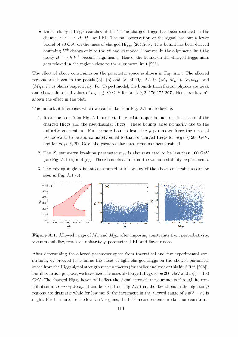
• Direct charged Higgs searches at LEP: The charged Higgs has been searched in the
channel e+e− → H+H− at LEP. The null observation of the signal has put a lower
bound of 80 GeV on the mass of charged Higgs [204,205]. This bound has been derived
assuming H± decays only to the τ ν and cs modes. However, in the alignment limit the
decay H± → hW± becomes significant. Hence, the bound on the charged Higgs mass
gets relaxed in the regions close to the alignment limit [206].
The effect of above constraints on the parameter space is shown in Fig. A.1 . The allowed
regions are shown in the panels (a), (b) and (c) of Fig. A.1 in (MA,MH±), (α,m12) and
(MH± ,m12) planes respectively. For Type-I model, the bounds from flavour physics are weak
and allows almost all values of mH± & 80 GeV for tanβ & 2 [176,177,207]. Hence we haven’t
shown the effect in the plot.
The important inferences which we can make from Fig. A.1 are following:
1. It can be seen from Fig. A.1 (a) that there exists upper bounds on the masses of the
charged Higgs and the pseudoscalar Higgs. These bounds arise primarily due to the
unitarity constraints. Furthermore bounds from the ρ parameter force the mass of
pseudoscalar to be approximately equal to that of charged Higgs for mH± & 200 GeV,
and for mH± . 200 GeV, the pseudoscalar mass remains unconstrained.
2. The Z2 symmetry breaking parameter m12 is also restricted to be less than 100 GeV
(see Fig. A.1 (b) and (c)). These bounds arise from the vacuum stability requirements.
3. The mixing angle α is not constrained at all by any of the above constraint as can be
seen in Fig. A.1 (c).
(a)
0 100 200 300 400 500 600
0
100
200
300
400
500
600
MA
MH±
Figure A.1: Allowed range of MA and MH± after imposing constraints from perturbativity,
vacuum stability, tree-level unitarity, ρ-parameter, LEP and flavour data.
After determining the allowed parameter space from theoretical and few experimental con-
straints, we proceed to examine the effect of light charged Higgs on the allowed parameter
space from the Higgs signal strength measurements (for earlier analyses of this kind Ref. [208]).
For illustration purpose, we have fixed the mass of charged Higgs to be 200 GeV andm212 = 100
GeV. The charged Higgs boson will affect the signal strength measurements through its con-
tribution in H → γγ decay. It can be seen from Fig A.2 that the deviations in the high tanβ
regions are dramatic while for low tanβ, the increment in the allowed range of sin(β − α) is
slight. Furthermore, for the low tanβ regions, the LEP measurements are far more constrain-
110
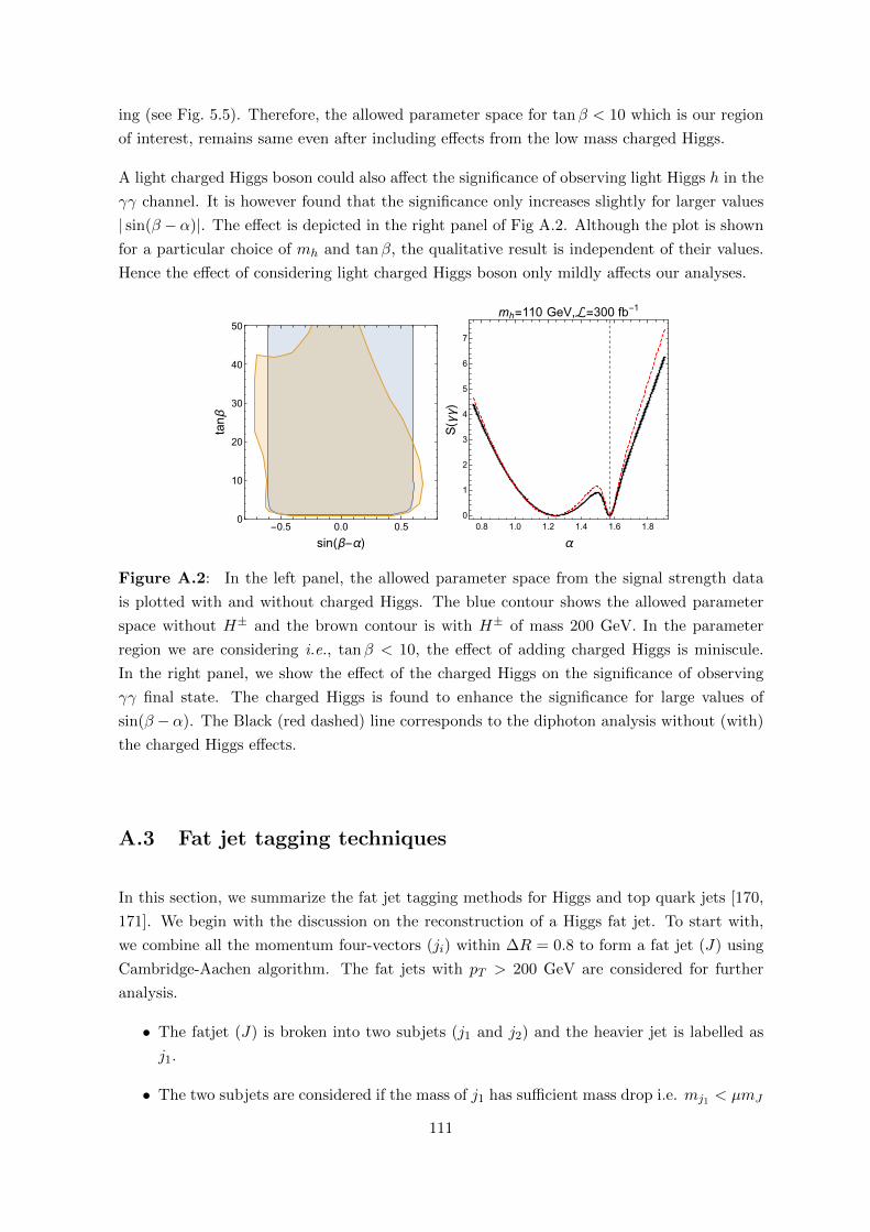
ing (see Fig. 5.5). Therefore, the allowed parameter space for tanβ < 10 which is our region
of interest, remains same even after including effects from the low mass charged Higgs.
A light charged Higgs boson could also affect the significance of observing light Higgs h in the
γγ channel. It is however found that the significance only increases slightly for larger values
| sin(β − α)|. The effect is depicted in the right panel of Fig A.2. Although the plot is shown
for a particular choice of mh and tanβ, the qualitative result is independent of their values.
Hence the effect of considering light charged Higgs boson only mildly affects our analyses.
-0.5 0.0 0.50
10
20
30
40
50
sin(β-α)
tanβ
0.8 1.0 1.2 1.4 1.6 1.8
0
1
2
3
4
5
6
7
α
S(γγ)
mh=110 GeV,ℒ=300 fb-1
Figure A.2: In the left panel, the allowed parameter space from the signal strength data
is plotted with and without charged Higgs. The blue contour shows the allowed parameter
space without H± and the brown contour is with H± of mass 200 GeV. In the parameter
region we are considering i.e., tanβ < 10, the effect of adding charged Higgs is miniscule.
In the right panel, we show the effect of the charged Higgs on the significance of observing
γγ final state. The charged Higgs is found to enhance the significance for large values of
sin(β − α). The Black (red dashed) line corresponds to the diphoton analysis without (with)
the charged Higgs effects.
A.3 Fat jet tagging techniques
In this section, we summarize the fat jet tagging methods for Higgs and top quark jets [170,
171]. We begin with the discussion on the reconstruction of a Higgs fat jet. To start with,
we combine all the momentum four-vectors (ji) within ∆R = 0.8 to form a fat jet (J) using
Cambridge-Aachen algorithm. The fat jets with pT > 200 GeV are considered for further
analysis.
• The fatjet (J) is broken into two subjets (j1 and j2) and the heavier jet is labelled as
j1.
• The two subjets are considered if the mass of j1 has sufficient mass drop i.e. mj1 < µmJ
111
and the splitting between two jets defined as y =min(pT1 , pT2)
max(pT1 , pT2)is greater than ycut
2.
This is a powerful cut to reduce the contaminations due to the QCD background. We
have considered µ = 0.67 and ycut = 0.09 for our analysis [170].
• If the previous condition is not satisfied then j1 is identified as J and the procedure is
repeated until both of the above conditions are satisfied.
• The final jet is considered as the Higgs if both subjets are b-tagged and the mass of the
filtered3 fat jet (mJ) is close to the Higgs mass.
Now we discuss the reconstruction of top jet. We combine all the momentum four-vectors
(ji) within ∆R = 1.2 to form a fat jet (J) using Cambridge-Achen algorithm. The fat jets
with pT > 250 GeV are considered for further analysis.
• Inside a fat jet, a lose massdrop criteria is employed such that J → j1j2, mj2 < mj1
and mj2 > 0.2mJ . The splitting takes place iteratively till mj1 > 30 GeV. A fat jet is
retained if it has atleast three such subjets.
• The three subjets are then filtered with ∆R = 0.3 into five subjets. Only those fatjets
with total jet mass close to the top quark mass are considered. The subjets which
reconstruct the top mass are then reclustered into three subjets.
• These subjets are then required to satisfy decay kinematics. Among three pair of in-
variant mass with these subjets, two of them are independent (as one of them satisfies
W-mass criteria). In a two dimensional space where the coordinates represent two inde-
pendent invariant mass, top-like jets represent a thin triangular annulus whereas QCD
jet is localized in the region of small pair-wise invariant mass.
A.4 Cross section
The dependency of the total cross section (σ× BR) on α and sin(β−α) are listed in Table. A.1
and also displayed in Fig. A.3.
It can be easily seen from the expressions of the cases A and D listed in the Table A.1, that
the behaviour of total cross section for pp→ h→ γγ and pp→Wh→Wbb becomes identical
with respect to α in the large tanβ regions. The same can also be verified from tanβ = 6
line Fig. A.3.
2 This is to ensure not too asymmetric splitting between j1 and j2.3To eliminate underlying events in the fatjet, it is filtered with Rfilter = 0.3 and three hard subjets are
retained.
112
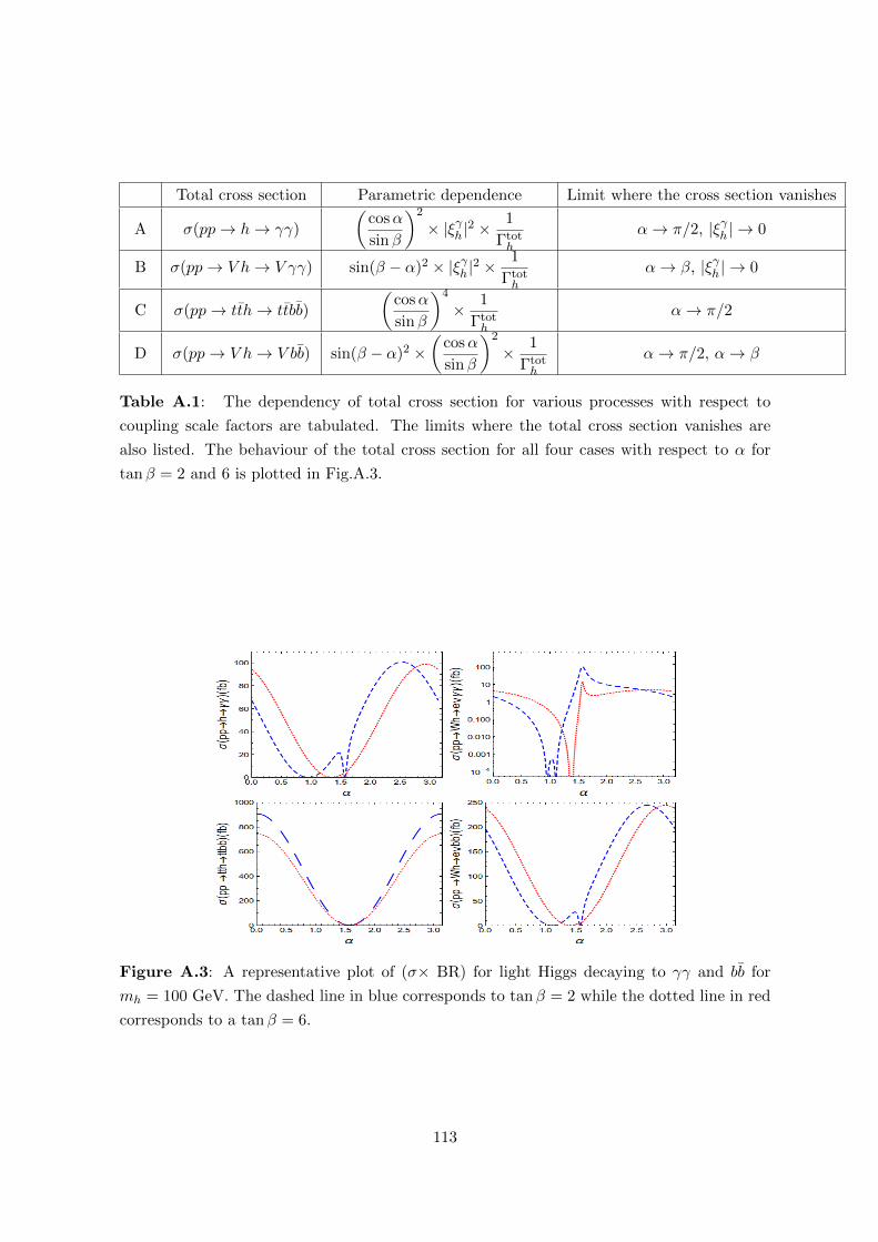
Total cross section Parametric dependence Limit where the cross section vanishes
A σ(pp→ h→ γγ)
(cosα
sinβ
)2
× |ξγh |2 ×1
Γtoth
α→ π/2, |ξγh | → 0
B σ(pp→ V h→ V γγ) sin(β − α)2 × |ξγh |2 ×1
Γtoth
α→ β, |ξγh | → 0
C σ(pp→ tth→ ttbb)
(cosα
sinβ
)4
× 1
Γtoth
α→ π/2
D σ(pp→ V h→ V bb) sin(β − α)2 ×(
cosα
sinβ
)2
× 1
Γtoth
α→ π/2, α→ β
Table A.1: The dependency of total cross section for various processes with respect to
coupling scale factors are tabulated. The limits where the total cross section vanishes are
also listed. The behaviour of the total cross section for all four cases with respect to α for
tanβ = 2 and 6 is plotted in Fig.A.3.
Figure A.3: A representative plot of (σ× BR) for light Higgs decaying to γγ and bb for
mh = 100 GeV. The dashed line in blue corresponds to tanβ = 2 while the dotted line in red
corresponds to a tanβ = 6.
113
Bibliography
[1] S. L. Glashow, Nucl. Phys. 22, 579 (1961).
[2] S. Weinberg, Phys. Rev. Lett. 19, 1264 (1967).
[3] Abdus Salam, Nobel Lecture, https://www.nobelprize.org/prizes/physics/1979/salam/lecture.
[4] D. J. Griffiths, “Introduction To Elementary Particles”.
[5] M. E. Peskin and D. V. Schroeder, “An Introduction to quantum field theory”.
[6] T. P. Cheng and L. F. Li, “Gauge Theory Of Elementary Particle Physics”.
[7] M. D. Schwartz, “Quantum Field Theory and the Standard Model”.
[8] Palash B. Pal, “An Introductory Course of Particle Physics”.
[9] F. Englert and R. Brout, Phys. Rev. Lett. 13, 321 (1964).
[10] P. W. Higgs, Phys. Rev. Lett. 13, 508 (1964).
[11] G. ’t Hooft, Nucl. Phys. B 35, 167 (1971).
[12] T. D. Lee and C. N. Yang, Phys. Rev. 104, 254 (1956).
[13] R. P. Feynman and M. Gell-Mann, Phys. Rev. 109, 193 (1958).
[14] E. C. G. Sudarshan and R. e. Marshak, Phys. Rev. 109, 1860 (1958).
[15] F. J. Hasert et al. [Gargamelle Neutrino Collaboration], Phys. Lett. B 46, 138 (1973)
[Phys. Lett. 46B, 138 (1973)].
[16] F. J. Hasert et al., Phys. Lett. B 46, 121 (1973) [Phys. Lett. 46B, 121 (1973)].
[17] R. Barate et al. [ALEPH and DELPHI and L3 and OPAL Collaborations and
LEP Working Group for Higgs boson searches], Phys. Lett. B 565, 61 (2003) [hep-
ex/0306033].
[18] C. E. Gerber et al. [TeV4LHC-Top Collaboration and Electroweak Working Group],
arXiv:0705.3251 [hep-ph].
[19] A. J. Bevan et al. [BaBar and Belle Collaborations], Eur. Phys. J. C 74, 3026 (2014).
[20] G. Aad et al. [ATLAS Collaboration], Phys. Lett. B 716, 1 (2012) ;
S. Chatrchyan et al. [CMS Collaboration], Phys. Lett. B 716, 30 (2012).
114
[21] G. Aad et al. [ATLAS and CMS Collaborations], JHEP 1608, 045 (2016).
[22] https://twiki.cern.ch/twiki/bin/view/CMSPublic/PhysicsResultsCombined,
https://twiki.cern.ch/twiki/bin/view/AtlasPublic/StandardModelPublicResults.
[23] See, for example, J. Ellis, Phil. Trans. Roy. Soc. Lond. A 370, 818 (2012).
[24] R. K. Kaul, arXiv:0803.0381 [hep-ph].
[25] https://pitp.ias.edu/sites/pitp/files/craig.pdf.
[26] R. Barbieri and A. Strumia, hep-ph/0007265.
[27] F. Capozzi, E. Lisi, A. Marrone, D. Montanino and A. Palazzo, “Neutrino masses and
mixings: Status of known and unknown 3ν parameters,” Nucl. Phys. B 908, 218 (2016).
[arXiv:1601.07777 [hep-ph]].
[28] I. Esteban, M. C. Gonzalez-Garcia, M. Maltoni, I. Martinez-Soler and T. Schwetz, “Up-
dated fit to three neutrino mixing: exploring the accelerator-reactor complementarity,”
arXiv:1611.01514 [hep-ph].
[29] http://pdg.lbl.gov/2018/reviews/rpp2018-rev-dark-matter.pdf.
[30] R. Aaij et al. [LHCb Collaboration], “Measurement of Form-Factor-Independent Ob-
servables in the Decay B0 → K∗0µ+µ−,” Phys. Rev. Lett. 111, 191801 (2013).
[31] R. Aaij et al. [LHCb Collaboration], “Angular analysis of the B0 → K∗0µ+µ− decay
using 3 fb−1 of integrated luminosity,” JHEP 1602, 104 (2016).
[32] R. Aaij et al. [LHCb Collaboration], “Test of lepton universality using B+ → K+`+`−
decays,” Phys. Rev. Lett. 113 (2014) 151601.
[33] R. Aaij et al. [LHCb Collaboration], JHEP 1708, 055 (2017).
[34] V. Khachatryan et al. [CMS Collaboration], Phys. Lett. B 767, 147 (2017).
[35] The ATLAS collaboration [ATLAS Collaboration], ATLAS-CONF-2016-059.
[36] V. Barger, P. Langacker, M. McCaskey, M. Ramsey-Musolf and G. Shaughnessy, Phys.
Rev. D 79, 015018 (2009).
[37] G. C. Branco, P. M. Ferreira, L. Lavoura, M. N. Rebelo, M. Sher and J. P. Silva,
“Theory and phenomenology of two-Higgs-doublet models,” Phys. Rept. 516, 1 (2012).
[38] P. Langacker, “The Physics of Heavy Z ′ Gauge Bosons,” Rev. Mod. Phys. 81, 1199
(2009).
[39] See for example, http://www.people.fas.harvard.edu/ hgeorgi/review.pdf.
[40] V. Khachatryan et al. [CMS and LHCb Collaborations], Nature 522, 68 (2015).
[41] A. Arbey, M. Battaglia, F. Mahmoudi and D. Martnez Santos, Phys. Rev. D 87, no. 3,
035026 (2013).
115
[42] A. Dighe, D. Ghosh, K. M. Patel and S. Raychaudhuri, Int. J. Mod. Phys. A 28, 1350134
(2013).
[43] G. Isidori, Y. Nir and G. Perez, Ann. Rev. Nucl. Part. Sci. 60, 355 (2010)
[44] C. Bobeth, G. Hiller and G. Piranishvili, “Angular distributions of B → K`+`− decays,”
JHEP 0712, 040 (2007).
[45] R. Aaij et al. [LHCb Collaboration], Phys. Rev. Lett. 118, no. 19, 191801 (2017).
[46] A. J. Buras, In *Lake Louise 1999, Electroweak physics* 1-83 [hep-ph/9905437].
[47] V. Ilisie,
[48] S. Descotes-Genon, J. Matias, M. Ramon and J. Virto, “Implications from clean ob-
servables for the binned analysis of B− > K ∗ µ+µ− at large recoil,” JHEP 1301, 048
(2013). [arXiv:1207.2753 [hep-ph]].
[49] S. Wehle et al. [Belle Collaboration], “Lepton-Flavor-Dependent Angular Analysis of
B → K∗`+`−,” arXiv:1612.05014 [hep-ex].
[50] R. Aaij et al. [LHCb Collaboration], “Differential branching fractions and isospin asym-
metries of B → K(∗)µ+µ− decays,” JHEP 1406, 133 (2014).
[51] R. Aaij et al. [LHCb Collaboration], “Differential branching fraction and angular anal-
ysis of the decay B0s → φµ+µ−,” JHEP 1307, 084 (2013).
[52] M. Bordone, G. Isidori and A. Pattori, “On the Standard Model predictions for RK
and RK∗ ,” Eur. Phys. J. C 76, no. 8, 440 (2016).
[53] G. Buchalla, A. J. Buras and M. E. Lautenbacher, “Weak decays beyond leading loga-
rithms,” Rev. Mod. Phys. 68, 1125 (1996) [hep-ph/9512380].
[54] W. Altmannshofer, P. Ball, A. Bharucha, A. J. Buras, D. M. Straub and M. Wick,
“Symmetries and Asymmetries of B → K∗µ+µ− Decays in the Standard Model and
Beyond,” JHEP 0901, 019 (2009).
[55] G. Hiller and F. Kruger, “More model independent analysis of b→ s processes,” Phys.
Rev. D 69, 074020 (2004) [hep-ph/0310219].
[56] G. Hiller and M. Schmaltz, “RK and future b→ s`` physics beyond the standard model
opportunities,” Phys. Rev. D 90, 054014 (2014).
[57] S. Descotes-Genon, J. Matias and J. Virto, “Understanding the B → K∗µ+µ−
Anomaly,” Phys. Rev. D 88, 074002 (2013).
[58] D. Ghosh, M. Nardecchia and S. A. Renner, “Hint of Lepton Flavour Non-Universality
in B Meson Decays,” JHEP 1412, 131 (2014).
[59] W. Altmannshofer and D. M. Straub, “New physics in b→ s transitions after LHC run
1,” Eur. Phys. J. C 75, no. 8, 382 (2015).
116
[60] S. Descotes-Genon, L. Hofer, J. Matias and J. Virto, “Global analysis of b → s``
anomalies,” JHEP 1606, 092 (2016).
[61] T. Hurth, F. Mahmoudi and S. Neshatpour, “On the anomalies in the latest LHCb
data,” Nucl. Phys. B 909, 737 (2016).
[62] R. Gauld, F. Goertz and U. Haisch, “On minimal Z ′ explanations of the B → K∗µ+µ−
anomaly,” Phys. Rev. D 89, 015005 (2014).
[63] S. L. Glashow, D. Guadagnoli and K. Lane, “Lepton Flavor Violation in B Decays?,”
Phys. Rev. Lett. 114, 091801 (2015).
[64] B. Bhattacharya, A. Datta, D. London and S. Shivashankara, “Simultaneous Explana-
tion of the RK and R(D(∗)) Puzzles,” Phys. Lett. B 742, 370 (2015).
[65] A. Crivellin, G. D’Ambrosio and J. Heeck, “Explaining h→ µ±τ∓, B → K∗µ+µ− and
B → Kµ+µ−/B → Ke+e− in a two-Higgs-doublet model with gauged Lµ−Lτ ,” Phys.
Rev. Lett. 114, 151801 (2015).
[66] A. Crivellin, G. D’Ambrosio and J. Heeck, “Addressing the LHC flavor anomalies with
horizontal gauge symmetries,” Phys. Rev. D 91, no. 7, 075006 (2015).
[67] A. Crivellin, L. Hofer, J. Matias, U. Nierste, S. Pokorski and J. Rosiek, “Lepton-flavour
violating B decays in generic Z ′ models,” Phys. Rev. D 92, no. 5, 054013 (2015).
[68] A. Celis, J. Fuentes-Martin, M. Jung and H. Serodio, “Family nonuniversal Z ′ models
with protected flavor-changing interactions,” Phys. Rev. D 92, no. 1, 015007 (2015).
[69] D. Aristizabal Sierra, F. Staub and A. Vicente, “Shedding light on the b→ s anomalies
with a dark sector,” Phys. Rev. D 92, no. 1, 015001 (2015).
[70] G. Blanger, C. Delaunay and S. Westhoff, “A Dark Matter Relic From Muon Anoma-
lies,” Phys. Rev. D 92, 055021 (2015).
[71] B. Gripaios, M. Nardecchia and S. A. Renner, “Linear flavour violation and anomalies
in B physics,” JHEP 1606, 083 (2016).
[72] B. Allanach, F. S. Queiroz, A. Strumia and S. Sun, “Z ′ models for the LHCb and g− 2
muon anomalies,” Phys. Rev. D 93, no. 5, 055045 (2016).
[73] K. Fuyuto, W. S. Hou and M. Kohda, “Z ′ -induced FCNC decays of top, beauty, and
strange quarks,” Phys. Rev. D 93, no. 5, 054021 (2016).
[74] C. W. Chiang, X. G. He and G. Valencia, “Z ′ model for b → s`` flavor anomalies,”
Phys. Rev. D 93, no. 7, 074003 (2016).
[75] S. M. Boucenna, A. Celis, J. Fuentes-Martin, A. Vicente and J. Virto, “Non-abelian
gauge extensions for B-decay anomalies,” Phys. Lett. B 760, 214 (2016).
117
[76] S. M. Boucenna, A. Celis, J. Fuentes-Martin, A. Vicente and J. Virto, “Phenomenology
of an SU(2)× SU(2)×U(1) model with lepton-flavour non-universality,” JHEP 1612,
059 (2016).
[77] A. Celis, W. Z. Feng and M. Vollmann, “Dirac Dark Matter and b→ s`+`− with U(1)
gauge symmetry,” arXiv:1608.03894 [hep-ph].
[78] W. Altmannshofer, S. Gori, S. Profumo and F. S. Queiroz, “Explaining dark matter
and B decay anomalies with an Lµ − Lτ model,” JHEP 1612, 106 (2016).
[79] A. Crivellin, J. Fuentes-Martin, A. Greljo and G. Isidori, “Lepton Flavor Non-
Universality in B decays from Dynamical Yukawas,” Phys. Lett. B 766, 77 (2017).
[80] I. Garcia Garcia, “LHCb anomalies from a natural perspective,” arXiv:1611.03507 [hep-
ph].
[81] D. Beirevi, O. Sumensari and R. Zukanovich Funchal, “Lepton flavor violation in ex-
clusive b→ s decays,” Eur. Phys. J. C 76, no. 3, 134 (2016).
[82] B. Bhattacharya, A. Datta, J. P. Guvin, D. London and R. Watanabe, “Simultaneous
Explanation of the RK and RD(∗) Puzzles: a Model Analysis,” arXiv:1609.09078 [hep-
ph].
[83] S. Biswas, D. Chowdhury, S. Han and S. J. Lee, “Explaining the lepton non-universality
at the LHCb and CMS within a unified framework,” JHEP 1502, 142 (2015).
[84] B. Gripaios, M. Nardecchia and S. A. Renner, “Composite leptoquarks and anomalies
in B-meson decays,” JHEP 1505, 006 (2015).
[85] S. Sahoo and R. Mohanta, “Scalar leptoquarks and the rare B meson decays,” Phys.
Rev. D 91, no. 9, 094019 (2015).
[86] D. Beirevi, S. Fajfer and N. Konik, “Lepton flavor nonuniversality in b → s`+`− pro-
cesses,” Phys. Rev. D 92, no. 1, 014016 (2015).
[87] R. Alonso, B. Grinstein and J. Martin Camalich, “Lepton universality violation and
lepton flavor conservation in B-meson decays,” JHEP 1510, 184 (2015).
[88] L. Calibbi, A. Crivellin and T. Ota, “Effective Field Theory Approach to b → s``′,
B → K ∗ νv and B → D∗τν with Third Generation Couplings,” Phys. Rev. Lett. 115,
181801 (2015).
[89] W. Huang and Y. L. Tang, “Flavor anomalies at the LHC and the R-parity violating
supersymmetric model extended with vectorlike particles,” Phys. Rev. D 92, no. 9,
094015 (2015).
[90] H. Ps and E. Schumacher, “Common origin of RK and neutrino masses,” Phys. Rev. D
92, no. 11, 114025 (2015).
118
[91] M. Bauer and M. Neubert, “Minimal Leptoquark Explanation for the RD(∗) , RK , and
(g − 2)g Anomalies,” Phys. Rev. Lett. 116, no. 14, 141802 (2016).
[92] S. Fajfer and N. Konik, “Vector leptoquark resolution of RK and RD(∗) puzzles,” Phys.
Lett. B 755, 270 (2016).
[93] R. Barbieri, G. Isidori, A. Pattori and F. Senia, “Anomalies in B-decays and U(2)
flavour symmetry,” Eur. Phys. J. C 76, no. 2, 67 (2016).
[94] S. Sahoo and R. Mohanta, “Lepton flavor violating B meson decays via a scalar lepto-
quark,” Phys. Rev. D 93, no. 11, 114001 (2016).
[95] I. Dorner, S. Fajfer, A. Greljo, J. F. Kamenik and N. Konik, “Physics of leptoquarks in
precision experiments and at particle colliders,” Phys. Rept. 641, 1 (2016).
[96] D. Das, C. Hati, G. Kumar and N. Mahajan, “Towards a unified explanation of RD(∗) ,
RK and (g − 2)µ anomalies in a left-right model with leptoquarks,” Phys. Rev. D 94,
055034 (2016).
[97] S. Sahoo and R. Mohanta, “Effects of scalar leptoquark on semileptonic Λb decays,”
New J. Phys. 18, no. 9, 093051 (2016).
[98] C. H. Chen, T. Nomura and H. Okada, “B → K∗µ+µ−, muon g − 2, and 750 GeV
diphoton excesses in a leptoquark model,” Phys. Rev. D 94, no. 11, 115005 (2016).
[99] D. Beirevi, N. Konik, O. Sumensari and R. Zukanovich Funchal, “Palatable Leptoquark
Scenarios for Lepton Flavor Violation in Exclusive b→ s`1`2 modes,” JHEP 1611, 035
(2016).
[100] D. Beirevi, S. Fajfer, N. Konik and O. Sumensari, “Leptoquark model to explain the
B-physics anomalies, RK and RD,” Phys. Rev. D 94, no. 11, 115021 (2016).
[101] S. Sahoo, R. Mohanta and A. K. Giri, “Explaining the RK and RD(∗) anomalies with
vector leptoquarks,” Phys. Rev. D 95, no. 3, 035027 (2017).
[102] R. Barbieri, C. W. Murphy and F. Senia, “B-decay Anomalies in a Composite Lepto-
quark Model,” Eur. Phys. J. C 77, no. 1, 8 (2017).
[103] P. Cox, A. Kusenko, O. Sumensari and T. T. Yanagida, “SU(5) Unification with TeV-
scale Leptoquarks,” arXiv:1612.03923 [hep-ph].
[104] L. Lavoura, “Zeros of the inverted neutrino mass matrix,” Phys. Lett. B 609, 317
(2005).
[105] E. I. Lashin and N. Chamoun, “Zero minors of the neutrino mass matrix,” Phys. Rev.
D 78, 073002 (2008).
[106] T. Araki, J. Heeck and J. Kubo, “Vanishing Minors in the Neutrino Mass Matrix from
Abelian Gauge Symmetries,” JHEP 1207, 083 (2012).
[107] J. Heeck, “Gauged Flavor Symmetries,” Nucl. Phys. Proc. Suppl. 237-238, 336 (2013).
119
[108] E. I. Lashin and N. Chamoun, “One vanishing minor in the neutrino mass matrix,”
Phys. Rev. D 80, 093004 (2009).
[109] D. Atwood, S. Bar-Shalom and A. Soni, Phys. Rev. D 76, 033004 (2007).
[110] A. J. Buras, “Weak Hamiltonian, CP violation and rare decays,” hep-ph/9806471.
[111] UTFIT collaboration, summer 2016 results, http://www.utfit.org
[112] A. J. Buras, J. Girrbach-Noe, C. Niehoff and D. M. Straub, “B → K(∗)νν decays in
the Standard Model and beyond,” JHEP 1502, 184 (2015).
[113] The ATLAS collaboration [ATLAS Collaboration], “Search for new high-mass reso-
nances in the dilepton final state using proton-proton collisions at√s = 13 TeV with
the ATLAS detector,” ATLAS-CONF-2016-045.
[114] CMS Collaboration [CMS Collaboration], “Search for a high-mass resonance decaying
into a dilepton final state in 13 fb−1 of pp collisions at√s = 13 TeV,” CMS-PAS-EXO-
16-031.
[115] G. Aad et al. [ATLAS Collaboration], “Search for new phenomena in dijet mass and
angular distributions from pp collisions at√s = 13 TeV with the ATLAS detector,”
Phys. Lett. B 754, 302 (2016).
[116] A. M. Sirunyan et al. [CMS Collaboration], “Search for dijet resonances in proton-
proton collisions at√s = 13 TeV and constraints on dark matter and other models,”
[arXiv:1611.03568 [hep-ex]].
[117] H. Fritzsch, Z. z. Xing and S. Zhou, “Two-zero Textures of the Majorana Neutrino Mass
Matrix and Current Experimental Tests,” JHEP 1109, 083 (2011).
[118] E. Ma, “Connection between the neutrino seesaw mechanism and properties of the
Majorana neutrino mass matrix,” Phys. Rev. D 71, 111301 (2005).
[119] M. Agostini et al. [GERDA Collaboration], “Results on Neutrinoless Double-β Decay
of 76Ge from Phase I of the GERDA Experiment,” Phys. Rev. Lett. 111, no. 12, 122503
(2013).
[120] Particle Data Group webpage, http://pdg.lbl.gov/2016/listings/
rpp2016-list-neutrino-prop.pdf
[121] S. Antusch, E. Cazzato and O. Fischer, arXiv:1612.02728 [hep-ph].
[122] A. Alloul, N. D. Christensen, C. Degrande, C. Duhr and B. Fuks, “FeynRules 2.0 - A
complete toolbox for tree-level phenomenology,” Comput. Phys. Commun. 185, 2250
(2014).
[123] J. Alwall et al., “The automated computation of tree-level and next-to-leading order
differential cross sections, and their matching to parton shower simulations,” JHEP
1407, 079 (2014).
120
[124] T. Sjostrand, S. Mrenna and P. Z. Skands, “PYTHIA 6.4 Physics and Manual,” JHEP
0605, 026 (2006).
[125] J. Pumplin, D. R. Stump, J. Huston, H. L. Lai, P. M. Nadolsky and W. K. Tung, “New
generation of parton distributions with uncertainties from global QCD analysis,” JHEP
0207, 012 (2002).
[126] S. Ovyn, X. Rouby and V. Lemaitre, “DELPHES, a framework for fast simulation of a
generic collider experiment,” arXiv:0903.2225 [hep-ph].
[127] J. de Favereau et al. [DELPHES 3 Collaboration], “DELPHES 3, A modular framework
for fast simulation of a generic collider experiment,” JHEP 1402, 057 (2014).
[128] I. Antcheva et al., “ROOT: A C++ framework for petabyte data storage, statistical
analysis and visualization,” Comput. Phys. Commun. 180, 2499 (2009).
[129] V. Khachatryan et al. [CMS Collaboration], “Measurements of the differential produc-
tion cross sections for a Z boson in association with jets in pp collisions at√s = 8 TeV,”
[arXiv:1611.03844 [hep-ex]].
[130] D. G. d’Enterria et al. [CMS Collaboration], “CMS physics technical design report:
Addendum on high density QCD with heavy ions,” J. Phys. G 34, 2307 (2007).
[131] Y. Amhis et al. [Heavy Flavor Averaging Group (HFAG)], “Averages of b-hadron, c-
hadron, and τ -lepton properties as of summer 2014,” arXiv:1412.7515 [hep-ex].
[132] T. Aushev et al., “Physics at Super B Factory,” arXiv:1002.5012 [hep-ex].
[133] C. Bobeth, G. Hiller and G. Piranishvili, JHEP 0807, 106 (2008).
[134] D. Ghosh, Eur. Phys. J. C 77, no. 10, 694 (2017).
[135] A. Datta, J. Kumar, J. Liao and D. Marfatia, Phys. Rev. D 97, no. 11, 115038 (2018)
[136] ATLAS Collaboration, Summary Plot for SUSY,
https://atlas.web.cern.ch/Atlas/GROUPS/PHYSICS/CombinedSummaryPlots/
SUSY/ATLAS SUSY Summary/
ATLAS SUSY Summary.png ;
ATLAS Collaboration, Summary Plot for Exotics,
https://atlas.web.cern.ch/Atlas/GROUPS/PHYSICS/CombinedSummaryPlots/EXOTICS/ATLAS Exotics Summary/
ATLAS Exotics Summary.png ;
CMS Combined Summary Plot,
https://twiki.cern.ch/twiki/pub/CMSPublic/PhysicsResultsCombined/exo-limits ICHEP 2016.001.png.
[137] J. Hewett, Theory Summary, delivered at the 53rd Recontres de Moriond (La Thuile,
Italy), March 2018.
[138] W. Buchmuller and D. Wyler, Nucl. Phys. B 268, 621 (1986).
For a more recent review, see S. Dawson, TASI 2016 Lectures, arXiv:1712.07232 [hep-
ph].
121
[139] K. Hagiwara, R. D. Peccei, D. Zeppenfeld and K. Hikasa, Nucl. Phys. B 282, 253 (1987).
[140] K. Hagiwara, S. Ishihara, R. Szalapski and D. Zeppenfeld, Phys. Lett. B 283, 353
(1992).
[141] U. Baur and D. Zeppenfeld, Phys. Lett. B 201, 383 (1988).
[142] S. S. Biswal, R. M. Godbole, B. Mellado and S. Raychaudhuri, Phys. Rev. Lett. 109,
261801 (2012) ;
S. S. Biswal, M. Patra and S. Raychaudhuri, arXiv:1405.6056 [hep-ph] ;
A. Azatov, J. Elias-Miro, Y. Reyimuaji and E. Venturini, JHEP 1710, 027 (2017) ;
R. Li, X. M. Shen, K. Wang, T. Xu, L. Zhang and G. Zhu, arXiv:1711.05607 [hep-ph].
[143] G. Buchalla, O. Cata, R. Rahn and M. Schlaffer, Eur. Phys. J. C 73, 2589 (2013) ;
L. Bian, J. Shu and Y. Zhang, JHEP 1509, 206 (2015) ;
A. Rosca, Nucl. Part. Phys. Proc. 273-275, 2226 (2016) ;
J. D. Wells and Z. Zhang, Phys. Rev. D 93, 034001 (2016) ;
S. M. Etesami, S. Khatibi and M. Mohammadi Najafabadi, Eur. Phys. J. C 76, 533
(2016) ;
R. Rahaman and R. K. Singh, arXiv:1711.04551 [hep-ph] ;
A. Falkowski et al., JHEP 1702, 115 (2017) ;
Z. Zhang, Phys. Rev. Lett. 118, 011803 (2017).
[144] T. Corbett et al., Phys. Rev. Lett. 111, 011801 (2013) ;
A. Butter, et al, JHEP 1607, 152 (2016).
[145] D. R. Green, P. Meade and M. A. Pleier, Rev. Mod. Phys. 89, 035008 (2017).
[146] G. Gounaris et al., hep-ph/9601233.
[147] G. Panico, F. Riva and A. Wulzer, Phys. Lett. B 776, 473 (2018).
[148] See, for example, S. Schael et al. [ALEPH, DELPHI, L3 and OPAL, LEP Electroweak
Collaborations], Phys. Rept. 532, 119 (2013).
[149] See, for example, C. E. Gerber et al. [TeV4LHC-Top Collaboration and Electroweak
Working Group], arXiv:0705.3251 [hep-ph].
[150] F. Boudjema, K. Hagiwara, C. Hamzaoui and K. Numata, Phys. Rev. D 43, 2223 (1991)
;
D. Choudhury, J. Kalinowski and A. Kulesza, Phys. Lett. B 457, 193 (1999).
[151] M. Aaboud et al. [ATLAS Collaboration], Eur. Phys. J. C 77, 563 (2017).
[152] A. M. Sirunyan et al. [CMS Collaboration], Phys. Lett. B 772, 21 (2017).
[153] G. Aad et al. [ATLAS Collaboration], Phys. Rev. D 87, 112003 (2013) ;
Erratum: Phys. Rev. D 91, 119901 (2015).
122
[154] S. Chatrchyan et al. [CMS Collaboration], Phys. Lett. B 701, 535 (2011) ;
S. Chatrchyan et al. [CMS Collaboration], Phys. Rev. D 89, 092005 (2014).
[155] J. Ohnemus, Phys. Rev. D 47, 940 (1993) ;
A. Denner, S. Dittmaier, M. Hecht and C. Pasold, JHEP 1504, 018 (2015).
[156] J. Alwall, M. Herquet, F. Maltoni, O. Mattelaer and T. Stelzer, JHEP 1106, 128 (2011).
[157] T. Sjstrand, S. Mrenna and P. Skands, JHEP05 (2006) 026, Comput. Phys. Comm. 178
(2008) 852.
[158] J. de Favereau et al. [DELPHES 3 Collaboration], JHEP 1402, 057 (2014)
[159] J. Pumplin et al., JHEP 0207, 012 (2002).
[160] R. D. Ball et al., Nucl. Phys. B 867, 244 (2013).
[161] CMS Collaboration [CMS Collaboration], CMS-PAS-HIG-17-013.
[162] G. Aad et al. [ATLAS Collaboration], Phys. Lett. B 726, 120 (2013).
[163] S. Chatrchyan et al. [CMS Collaboration], Phys. Rev. D 89, no. 9, 092007 (2014).
[164] V. Khachatryan et al. [CMS Collaboration], Phys. Rev. D 92, no. 7, 072010 (2015).
[165] V. Khachatryan et al. [CMS Collaboration], JHEP 1710, 076 (2017).
[166] J. Bernon, J. F. Gunion, Y. Jiang and S. Kraml, Phys. Rev. D 91, no. 7, 075019 (2015).
[167] R. Aggleton, D. Barducci, N. E. Bomark, S. Moretti and C. Shepherd-Themistocleous,
JHEP 1702, 035 (2017).
[168] CMS Collaboration [CMS Collaboration], CMS-PAS-HIG-14-037.
[169] G. Aad et al. [ATLAS Collaboration], Phys. Rev. Lett. 113, no. 17, 171801 (2014).
[170] J. M. Butterworth, A. R. Davison, M. Rubin and G. P. Salam, Phys. Rev. Lett. 100,
242001 (2008).
[171] T. Plehn and M. Spannowsky, J. Phys. G 39, 083001 (2012).
[172] S. Nie and M. Sher, Phys. Lett. B 449, 89 (1999).
[173] A. G. Akeroyd, A. Arhrib and E. M. Naimi, Phys. Lett. B 490, 119 (2000).
[174] G. Bhattacharyya and D. Das, Pramana 87, no. 3, 40 (2016).
[175] S. Schael et al. [ALEPH and DELPHI and L3 and OPAL and SLD Collaborations and
LEP Electroweak Working Group and SLD Electroweak Group and SLD Heavy Flavour
Group], Phys. Rept. 427, 257 (2006).
[176] F. Mahmoudi and O. Stal, Phys. Rev. D 81, 035016 (2010).
[177] M. Aoki, S. Kanemura, K. Tsumura and K. Yagyu, Phys. Rev. D 80, 015017 (2009).
[178] J. F. Gunion, H. E. Haber, G. L. Kane and S. Dawson, Front. Phys. 80, 1 (2000).
123
[179] V. D. Barger and R. J. N. Phillips, “Collider Physics,” REDWOOD CITY, USA:
ADDISON-WESLEY (1987) 592 P. (FRONTIERS IN PHYSICS, 71).
[180] S. Dawson et al., arXiv:1310.8361 [hep-ex].
[181] G. Cacciapaglia, A. Deandrea, S. Gascon-Shotkin, S. Le Corre, M. Lethuillier and
J. Tao, JHEP 1612, 068 (2016).
[182] S. Schael et al. [ALEPH and DELPHI and L3 and OPAL Collaborations and LEP
Working Group for Higgs Boson Searches], Eur. Phys. J. C 47, 547 (2006).
[183] T. Aaltonen et al. [CDF Collaboration], Phys. Rev. D 87, 052008 (2013).
[184] [ALEPH and DELPHI and L3 and OPAL Collaborations and LEP Higgs Working
Group], hep-ex/0107030.
[185] J. Abdallah et al. [DELPHI Collaboration], Eur. Phys. J. C 35, 313 (2004).
[186] T. Sjstrand et al., Comput. Phys. Commun. 191, 159 (2015).
[187] R. D. Ball et al. [NNPDF Collaboration], Nucl. Phys. B 877, 290 (2013).
[188] M. Cacciari, G. P. Salam and G. Soyez, JHEP 0804, 063 (2008).
[189] S. D. Ellis, T. S. Roy and J. Scholtz, Phys. Rev. Lett. 110, no. 12, 122003 (2013).
[190] S. D. Ellis, T. S. Roy and J. Scholtz, Phys. Rev. D 87, no. 1, 014015 (2013).
[191] L. D. Landau, Dokl. Akad. Nauk Ser. Fiz. 60, no. 2, 207 (1948).
[192] C. N. Yang, Phys. Rev. 77, 242 (1950).
[193] M. Chala, M. Duerr, F. Kahlhoefer and K. Schmidt-Hoberg, Phys. Lett. B 755, 145
(2016).
[194] N. D. Christensen and C. Duhr, Comput. Phys. Commun. 180, 1614 (2009).
[195] M. Cacciari, G. P. Salam and G. Soyez, Eur. Phys. J. C 72, 1896 (2012).
[196] B. Bhattacherjee, S. Mukhopadhyay, M. M. Nojiri, Y. Sakaki and B. R. Webber, JHEP
1504, 131 (2015).
[197] J. Thaler and K. Van Tilburg, JHEP 1103, 015 (2011).
[198] J. Thaler and K. Van Tilburg, JHEP 1202, 093 (2012).
[199] A. J. Larkoski, G. P. Salam and J. Thaler, JHEP 1306, 108 (2013).
[200] A. Chakraborty, A. M. Iyer and T. S. Roy, Nucl. Phys. B 932, 439 (2018).
[201] C. Athanasiou, C. G. Lester, J. M. Smillie and B. R. Webber, JHEP 0608, 055 (2006).
[202] S. Kullback and R.A. Leibler, The annals of mathematical statistics, 22, 1, 79 (1951).
[203] D. A. Ross and J. C. Taylor, Nucl. Phys. B 51, 125 (1973) Erratum: [Nucl. Phys. B
58, 643 (1973)].
124

[204] [ALEPH and DELPHI and L3 and OPAL Collaborations and LEP Higgs Working
Group for Higgs boson searches], hep-ex/0107031.
[205] P. Abreu et al. [DELPHI Collaboration], Phys. Lett. B 507, 89 (2001).
[206] A. Arbey, F. Mahmoudi, O. Stal and T. Stefaniak, Eur. Phys. J. C 78, no. 3, 182 (2018).
[207] A. Arbey and F. Mahmoudi, Comput. Phys. Commun. 182, 1582 (2011).
[208] P. Posch, Phys. Lett. B 696, 447 (2011).
125


![F arXiv:2001.05986v1 [math.QA] 16 Jan 2020arXiv:2001.05986v1 [math.QA] 16 Jan 2020 BOSONIC GHOSTBUSTING — THE BOSONIC GHOST VERTEX ALGEBRA ADMITS A LOGARITHMIC MODULE CATEGORY WITH](https://img.dokumen.tips/doc/110x75/5f41e2b6ba2f5a5fa06b4c58/f-arxiv200105986v1-mathqa-16-jan-2020-arxiv200105986v1-mathqa-16-jan-2020.jpg)