Department of Science and Technology Institutionen för teknik och naturvetenskap Linköping University Linköpings universitet

gnipökrroN 47 106 nedewS ,gnipökrroN 47 106-ES

LiU-ITN-TEK-A-16/057--SE

Design och Implementering avett Out-of-Core

Globrenderingssystem Baseratpå Olika Karttjänster

Kalle Bladin

Erik Broberg

2016-12-02

LiU-ITN-TEK-A-16/057--SE

Design och Implementering avett Out-of-Core

Globrenderingssystem Baseratpå Olika Karttjänster

Examensarbete utfört i Medieteknikvid Tekniska högskolan vid

Linköpings universitet

Kalle BladinErik Broberg

Handledare Alexander BockExaminator Anders Ynnerman

Norrköping 2016-12-02

Upphovsrätt

Detta dokument hålls tillgängligt på Internet – eller dess framtida ersättare –under en längre tid från publiceringsdatum under förutsättning att inga extra-ordinära omständigheter uppstår.

Tillgång till dokumentet innebär tillstånd för var och en att läsa, ladda ner,skriva ut enstaka kopior för enskilt bruk och att använda det oförändrat förickekommersiell forskning och för undervisning. Överföring av upphovsrättenvid en senare tidpunkt kan inte upphäva detta tillstånd. All annan användning avdokumentet kräver upphovsmannens medgivande. För att garantera äktheten,säkerheten och tillgängligheten finns det lösningar av teknisk och administrativart.

Upphovsmannens ideella rätt innefattar rätt att bli nämnd som upphovsman iden omfattning som god sed kräver vid användning av dokumentet på ovanbeskrivna sätt samt skydd mot att dokumentet ändras eller presenteras i sådanform eller i sådant sammanhang som är kränkande för upphovsmannens litteräraeller konstnärliga anseende eller egenart.

För ytterligare information om Linköping University Electronic Press seförlagets hemsida http://www.ep.liu.se/

Copyright

The publishers will keep this document online on the Internet - or its possiblereplacement - for a considerable time from the date of publication barringexceptional circumstances.

The online availability of the document implies a permanent permission foranyone to read, to download, to print out single copies for your own use and touse it unchanged for any non-commercial research and educational purpose.Subsequent transfers of copyright cannot revoke this permission. All other usesof the document are conditional on the consent of the copyright owner. Thepublisher has taken technical and administrative measures to assure authenticity,security and accessibility.

According to intellectual property law the author has the right to bementioned when his/her work is accessed as described above and to be protectedagainst infringement.

For additional information about the Linköping University Electronic Pressand its procedures for publication and for assurance of document integrity,please refer to its WWW home page: http://www.ep.liu.se/

© Kalle Bladin, Erik Broberg

Master’s thesis

Design and Implementation of an

Out-of-Core Globe Rendering System Using

Multiple Map Services

Submitted in partial fulfillment of

the requirements for the award of the degree of

Master of Science

in

Media Technology and Engineering

Submitted by

Kalle Bladin & Erik Broberg

ExaminerAnders Ynnerman

SupervisorAlexander Bock

Department of Science and TechnologyLinköping University 2016

Abstract

This thesis focuses on the design and implementation of a software systemenabling out-of-core rendering of multiple map datasets mapped on virtualglobes around our solar system. Challenges such as precision, accuracy, cur-vature and massive datasets were considered. The result is a globe visual-ization software using a chunked level of detail approach for rendering. Thesoftware can render texture layers of various sorts to aid in scientific visual-ization on top of height mapped geometry, yielding accurate visualizationsrendered at interactive frame rates.

The project was conducted at the American Museum of Natural History(AMNH), New York and serves the goal of implementing a planetary visual-ization software to aid in public presentations and bringing space science tothe public.

The work is part of the development of the software OpenSpace, which isthe result of a collaboration between Linköping University, AMNH and theNational Aeronautics and Space Administration (NASA) among others.

Acknowledgments

We would like to give our sincerest thanks to all the people who have beeninvolved in making this thesis work possible. Thanks to Anders Ynnerman forgiving us this opportunity. Thanks to Carter Emmart for being an inspiringand driving force for the project and for sharing his passion in bringingknowledge and interest in astronomy to the general public. Thanks to VivianTrakinski for making us feel needed and useful within the Openspace projectand within the museum.

Thanks to Alexander Bock for his dedication in the project and the sup-port he has given as a mentor along with Emil Axelsson during the wholeproject. Thanks to all the people in the OpenSpace team, including ourpeers Michael and Sebastian, which have been both inspiring, helpful andenjoyable to work and share the experience with.

We would like to thank all the people we have met during our time atAMNH. Kayla, Eozin, Natalia have not only been our trusted lunch matesbut also great friends outside of work. Thanks to Jay for all the hardwaresupport, and also all the rest of the people at the Science Bulletins and RoseCenter Engineering for being so welcoming and helpful.

We would also like to thank Lucian Plesea for his expert support in map-ping services together with Vikram Singh for setting up the map serverswe could use in our software. Also, thanks to Jason, Ally and David forproviding us with high resolution Mars imagery data that we could use forrendering.

A big thank you to Masha and the rest of the CCMC team as well asRyan, who made our visit to NASA Goddard Space Flight Center the bestexperience possible by inspiring us and giving us insight in parts of NASA’sspace science.

All our friends and family who travelled from Sweden to visit us in NewYork, we’re happy for sharing a great time with you during our leisure.

Last but not least we are very happy to have made new great friendsoutside of the thesis work during our stay in the United States. You havemade this experience even more enjoyable.

1

Contents

Acknowledgements 1

1 Introduction 1

1.1 Background . . . . . . . . . . . . . . . . . . . . . . . . . . . . 11.1.1 OpenSpace . . . . . . . . . . . . . . . . . . . . . . . . 11.1.2 Globe Browsing . . . . . . . . . . . . . . . . . . . . . . 2

1.2 Objectives . . . . . . . . . . . . . . . . . . . . . . . . . . . . . 31.3 Delimitations . . . . . . . . . . . . . . . . . . . . . . . . . . . 41.4 Challenges . . . . . . . . . . . . . . . . . . . . . . . . . . . . . 5

2 Theoretical Background 6

2.1 Large Scale Map Datasets . . . . . . . . . . . . . . . . . . . . 62.1.1 Web Map Services . . . . . . . . . . . . . . . . . . . . 72.1.2 Georeferenced Image Formats . . . . . . . . . . . . . . 82.1.3 Available Imagery Products . . . . . . . . . . . . . . . 8

2.2 Modeling Globes . . . . . . . . . . . . . . . . . . . . . . . . . 102.2.1 Globes as Ellipsoids . . . . . . . . . . . . . . . . . . . . 102.2.2 Tessellating the Ellipsoid . . . . . . . . . . . . . . . . . 112.2.3 2D Parameterisation for Map Projections . . . . . . . . 14

2.3 Dynamic Level of Detail . . . . . . . . . . . . . . . . . . . . . 202.3.1 Discrete Level of Detail . . . . . . . . . . . . . . . . . . 212.3.2 Continuous Level of Detail . . . . . . . . . . . . . . . . 212.3.3 Hierarchical Level of Detail . . . . . . . . . . . . . . . 22

2.4 Level of Detail Algorithms for Globes . . . . . . . . . . . . . . 242.4.1 Chunked LOD . . . . . . . . . . . . . . . . . . . . . . . 242.4.2 Geometry Clipmaps . . . . . . . . . . . . . . . . . . . . 27

2.5 Precision Issues . . . . . . . . . . . . . . . . . . . . . . . . . . 312.5.1 Floating Point Numbers . . . . . . . . . . . . . . . . . 312.5.2 Single Precision Floating Point Numbers . . . . . . . . 312.5.3 Double Precision Floating Point Numbers . . . . . . . 322.5.4 Rendering Artifacts . . . . . . . . . . . . . . . . . . . . 32

i

2.6 Caching . . . . . . . . . . . . . . . . . . . . . . . . . . . . . . 342.6.1 Multi Stage Texture Caching . . . . . . . . . . . . . . 342.6.2 Cache Replacement Policies . . . . . . . . . . . . . . . 34

3 Implementation 36

3.1 Reference Ellipsoid . . . . . . . . . . . . . . . . . . . . . . . . 373.2 Chunked LOD . . . . . . . . . . . . . . . . . . . . . . . . . . . 37

3.2.1 Chunks . . . . . . . . . . . . . . . . . . . . . . . . . . 373.2.2 Chunk Selection . . . . . . . . . . . . . . . . . . . . . . 383.2.3 Chunk Tree Growth Limitation . . . . . . . . . . . . . 393.2.4 Chunk Culling . . . . . . . . . . . . . . . . . . . . . . . 40

3.3 Reading and Tiling Image Data . . . . . . . . . . . . . . . . . 413.3.1 GDAL . . . . . . . . . . . . . . . . . . . . . . . . . . . 423.3.2 Tile Dataset . . . . . . . . . . . . . . . . . . . . . . . . 443.3.3 Async Tile Dataset . . . . . . . . . . . . . . . . . . . . 46

3.4 Providing Tiles . . . . . . . . . . . . . . . . . . . . . . . . . . 483.4.1 Caching Tile Provider . . . . . . . . . . . . . . . . . . 493.4.2 Temporal Tile Provider . . . . . . . . . . . . . . . . . . 503.4.3 Single Image Tile Provider . . . . . . . . . . . . . . . . 513.4.4 Text Tile Provider . . . . . . . . . . . . . . . . . . . . 52

3.5 Mapping Tiles onto Chunks . . . . . . . . . . . . . . . . . . . 533.5.1 Chunk Tiles . . . . . . . . . . . . . . . . . . . . . . . . 533.5.2 Chunk Tile Pile . . . . . . . . . . . . . . . . . . . . . . 54

3.6 Managing Multiple Data Sources . . . . . . . . . . . . . . . . 553.6.1 Layers . . . . . . . . . . . . . . . . . . . . . . . . . . . 563.6.2 Layers on the GPU . . . . . . . . . . . . . . . . . . . . 56

3.7 Chunk Rendering . . . . . . . . . . . . . . . . . . . . . . . . . 603.7.1 Grid . . . . . . . . . . . . . . . . . . . . . . . . . . . . 603.7.2 Vertex Pipeline . . . . . . . . . . . . . . . . . . . . . . 613.7.3 Fragment Pipeline . . . . . . . . . . . . . . . . . . . . 633.7.4 Dynamic Shader Programs . . . . . . . . . . . . . . . . 643.7.5 LOD Switching . . . . . . . . . . . . . . . . . . . . . . 65

3.8 Interaction . . . . . . . . . . . . . . . . . . . . . . . . . . . . . 67

4 Results 68

4.1 Screenshots . . . . . . . . . . . . . . . . . . . . . . . . . . . . 684.1.1 Height Mapping . . . . . . . . . . . . . . . . . . . . . . 694.1.2 Water Masking . . . . . . . . . . . . . . . . . . . . . . 704.1.3 Night Layers . . . . . . . . . . . . . . . . . . . . . . . . 714.1.4 Color Overlays . . . . . . . . . . . . . . . . . . . . . . 724.1.5 Grayscale Overlaying . . . . . . . . . . . . . . . . . . . 73

ii

4.1.6 Local Patches . . . . . . . . . . . . . . . . . . . . . . . 744.1.7 Visualizing Scientific Parameters . . . . . . . . . . . . 754.1.8 Visual Debugging: Bounding Volumes . . . . . . . . . 764.1.9 Visual Debugging: Camera Frustum . . . . . . . . . . 77

4.2 Benchmarking . . . . . . . . . . . . . . . . . . . . . . . . . . . 784.2.1 Top Down Views . . . . . . . . . . . . . . . . . . . . . 794.2.2 Culling for Distance Based Chunk Selection . . . . . . 814.2.3 Culling for Area Based Chunk Selection . . . . . . . . 834.2.4 LOD: Distance Based vs. Area Based . . . . . . . . . . 854.2.5 Switching Using Level Blending . . . . . . . . . . . . . 864.2.6 Polar Pinching . . . . . . . . . . . . . . . . . . . . . . 884.2.7 Benchmark: Interactive Globe Browsing . . . . . . . . 894.2.8 Camera Space Rendering . . . . . . . . . . . . . . . . . 90

5 Discussion 91

5.1 Chunked LOD . . . . . . . . . . . . . . . . . . . . . . . . . . . 915.1.1 Chunk Culling . . . . . . . . . . . . . . . . . . . . . . . 915.1.2 Chunk Selection . . . . . . . . . . . . . . . . . . . . . . 925.1.3 Chunk Switching . . . . . . . . . . . . . . . . . . . . . 925.1.4 Inconsistent Globe Browsing Performance . . . . . . . 93

5.2 Ellipsoids vs Spheres . . . . . . . . . . . . . . . . . . . . . . . 945.3 Tessellation and Projection . . . . . . . . . . . . . . . . . . . . 945.4 Chunked LOD vs Ellipsoidal Clipmaps . . . . . . . . . . . . . 955.5 Parallel Tile Requests . . . . . . . . . . . . . . . . . . . . . . . 955.6 High Resolution Local Patches . . . . . . . . . . . . . . . . . . 96

6 Conclusions 97

7 Future Work 98

7.1 Parallelizing GDAL Requests . . . . . . . . . . . . . . . . . . 987.2 Browsing WMS Datasets Upon Request . . . . . . . . . . . . 987.3 Integrating Atmosphere Rendering . . . . . . . . . . . . . . . 987.4 Local Patches and Rover Terrains . . . . . . . . . . . . . . . . 997.5 Other Features . . . . . . . . . . . . . . . . . . . . . . . . . . 997.6 Other Uses of Chunked LOD Spheres in Astro-Visualization . 100

References 101

Appendices 106

A General Use of Globe Browsing in OpenSpace 107

iii

B Build Local DEM Patches to Load With OpenSpace 108

iv

List of Figures

2.1 The size of the map is decreasing exponentially with the overview.Figure adapted from [13] . . . . . . . . . . . . . . . . . . . . . 6

2.2 The WGS84 coordinate system and globe. Figure adaptedfrom [13] . . . . . . . . . . . . . . . . . . . . . . . . . . . . . . 11

2.3 Geographic grid tessellation of a sphere with constant numberof latitudinal segments of 4, 8 and 16 respectively . . . . . . . 12

2.4 Quadrilateralized spherical cube tessellation with 0, 1, 2 and3 subdivisions respectively . . . . . . . . . . . . . . . . . . . . 12

2.5 Hierarchical triangular mesh tessellation of a sphere with 0, 1,2 and 3 subdivisions respectively . . . . . . . . . . . . . . . . 13

2.6 HEALPix tessellation of three different levels of detail . . . . . 132.7 Geographic tessellation of a sphere with polar caps . . . . . . 142.8 Geographic map projection. Figure adapted from [13] . . . . . 152.9 Difference between geocentric latitudes, φc and geodetic lat-

itudes, φd for a point ~p on the surface of an ellipsoid. Thefigure also shows the difference between geocentric and geode-tic surface normals, n̂c and n̂d, respectively. . . . . . . . . . . . 16

2.10 Unwrapped equirectangular and mercator projections. Themercator projection works when it is unwrapped due to itbeing conformal (preserving aspect ratio). . . . . . . . . . . . 17

2.11 Mercator projection. Figure adapted from [13] . . . . . . . . . 172.12 Cube map projection. Figure adapted from [13] . . . . . . . . 182.13 TOAST map projection. Figure adapted from [13] . . . . . . . 192.14 HEALPix map projection. Figure adapted from [13] . . . . . . 192.15 Polar map projections. Figure adapted from [13] . . . . . . . . 202.16 A range of predefined meshes with increasing resolution. Dy-

namic level of detail algorithms are used to choose the mostsuitable mesh for rendering . . . . . . . . . . . . . . . . . . . . 21

2.17 Mesh operations in continous LOD . . . . . . . . . . . . . . . 222.18 Bunny model chunked up using HLOD. Child nodes represent

higher resolution representations of parts of the parent models 23

v

2.19 Chunked LOD for a globe . . . . . . . . . . . . . . . . . . . . 242.20 Culling for chunked LOD. Red chunks can be culled due to

them being invisible to the camera . . . . . . . . . . . . . . . 262.21 Vertex positions when switching between levels . . . . . . . . . 262.22 Chunks with skirts hide the undesired cracks between them . . 272.23 Clip maps are smaller than mip maps as only parts of the

complete map need to be stored. Figure adapted from [13] . . 282.24 The Geometry Clipmaps follow the view point. Higher levels

have coarser grids but covers smaller areas. The interior partof the grid can collapse so that higher level geometries cansnap to their grid . . . . . . . . . . . . . . . . . . . . . . . . . 28

2.25 Geometry Clipmaps on a geographic grid cause pinching aroundthe poles, which needs to be handled explicitly . . . . . . . . . 29

2.26 Jupiter’s moon Europa rendered with single precision floatingpoint operations. The precision errors in the placement of thevertices is apparent as jagged edges even at a distance far fromthe globe. . . . . . . . . . . . . . . . . . . . . . . . . . . . . . 33

2.27 Z-fighting as fragments flip between being behind or in frontof each other . . . . . . . . . . . . . . . . . . . . . . . . . . . 33

2.28 Inserting an entry in a LRU cache. . . . . . . . . . . . . . . . 35

3.1 Overviewing class diagram of RenderableGlobe and its relatedclasses. . . . . . . . . . . . . . . . . . . . . . . . . . . . . . . . 36

3.2 Triangle with the area 1/8 of the chunk projected onto a unitsphere. The area is used to approximate the solid angle of thechunk used as an error metric when selecting chunks to render 39

3.3 Frustum culling algorithm. This chunk cannot be frustumculled. . . . . . . . . . . . . . . . . . . . . . . . . . . . . . . . 40

3.4 Horizon culling is performed by comparing the length lh + lmwith the actual distance between the camera position and theobject at position ~p. . . . . . . . . . . . . . . . . . . . . . . . . 41

3.5 The required GDAL RasterIO parameters. . . . . . . . . . . . 433.6 Result of GDAL raster IO. . . . . . . . . . . . . . . . . . . . . 433.7 The tile dataset pipeline takes a tile index as input, interfaces

with GDAL and returns a raw tile . . . . . . . . . . . . . . . . 443.8 Overview of the calculation of an IO description. . . . . . . . . 453.9 Asynchronous reading of Raw tiles can be performed on sep-

arate threads. When the tile reading job is finished the rawtile will be appended to a concurrent queue. . . . . . . . . . . 47

3.10 Retrieving finished RawTiles. . . . . . . . . . . . . . . . . . . 473.11 Tile provider interface for accessing tiles . . . . . . . . . . . . 48

vi

3.12 Tiles are either provided from cache or enqueued in an asyn-chronous tile dataset if it is not available . . . . . . . . . . . . 49

3.13 The tile cache is updated once per frame . . . . . . . . . . . . 503.14 Tiles are fetched on demand. The first time a tile is re-

quested, the asynchronous tile dataset will request it on aworker thread. As soon as the tile has been initialized it willhave the status “OK” and can be used for rendering . . . . . . 50

3.15 Each temporal snapshot is internally represented by a cachingtile provider . . . . . . . . . . . . . . . . . . . . . . . . . . . . 51

3.16 Serving single tiles is useful for debugging chunk and texturealignment . . . . . . . . . . . . . . . . . . . . . . . . . . . . . 52

3.17 Serving tiles with custom text rendered on them can be usedas size references or providing other information. The tileprovider is internally holding a LRU cache for initialized tiles . 52

3.18 Only the highlighted subset of the parent tile is used for ren-dering the chunk. Figure adapted from [13] . . . . . . . . . . . 53

3.19 The image data of a given chunk tile pile. Only the highlightedsubset of the parent tiles are used for rendering the chunk.Figure from [28] . . . . . . . . . . . . . . . . . . . . . . . . . . 55

3.20 UML diagram of the LayerManager and its related classes . . 573.21 UML structure for corresponding GPU-mapped hierarchy. The

class GPUData<T> maintains an OpenGL uniform location . . . 583.22 Grid with skirts with a side of N = 4 segments. Green repre-

sents the main area with texture coordinates ∈ [0, 1] and blueis the skirt of the grid. . . . . . . . . . . . . . . . . . . . . . . 60

3.23 Model space rendering of chunks is performed with a mappingof vertices from geodetic coordinates to Cartesian coordinates. 61

3.24 Vertex pipeline for model space rendering. Variables on theCPU are defined in double precision and cast to single preci-sion before being uploaded to the GPU. . . . . . . . . . . . . . 61

3.25 Interpolating vertex positions in camera space leads to highprecision in the representation of vertex positions close to thecamera compared to positions defined in model space. . . . . . 62

3.26 Vertex pipeline for camera space rendering. Variables on theCPU are defined in double precision and cast to single preci-sion before being uploaded to the GPU . . . . . . . . . . . . . 62

3.27 Blending on a per fragment basis. The level interpolationparameter t is used to calculate level weights w1 = 1 − t andw2 = t, in this case using two chunk tiles per chunk tile pile. . 66

vii

4.1 Shaded Earth rendered with NASA GIBS VIIRS daily image[17] . . . . . . . . . . . . . . . . . . . . . . . . . . . . . . . . . 68

4.2 Earth rendered with ESRI World Elevation 3D height map[44]. Color layer: ESRI Imagery World 2D [28] . . . . . . . . . 69

4.3 Shaded Earth using water mask texture. Color layer: ESRIImagery World 2D [28] . . . . . . . . . . . . . . . . . . . . . . 70

4.4 Night layers are only rendered on the night side of the planet.Night layer: NASA GIBS VIIRS Earth at night [17] . . . . . . 71

4.5 Earth rendered with different color overlays used for reference.Color layer: ESRI Imagery World 2D [28] . . . . . . . . . . . . 72

4.6 Valles Marineris, Mars with different layers . . . . . . . . . . . 734.7 Local DTM patches of West Candor Chasma, Valles Marineris,

Mars. All figures use color layer: Viking MDIM [19] and heightlayer: MOLA [45]. . . . . . . . . . . . . . . . . . . . . . . . . 74

4.8 Visualization of scientific parameters on the globe. All thesedatasets are temporal and can be animated over time. Datasetsfrom [17]. . . . . . . . . . . . . . . . . . . . . . . . . . . . . . 75

4.9 Rendering the bounding polyhedra for chunks at Mars. Notehow the polyhedra start out as tetrahedra for the largest chunksin 4.9a and converge to rectangular blocks as seen in 4.9d. . . 76

4.10 Chunks culled outside the view frustum. The skirt length ofthe chunks differ depending on the level. The figure also showshow some chunks are rendered in model space (green edges)and some in camera space (red edges). . . . . . . . . . . . . . 77

4.11 Top down views of Earth at different altitudes . . . . . . . . . 794.12 As the camera descends towards the ground looking straight

down, the chunk tree grows but the number of rendered chunksremains relatively constant due to culling. . . . . . . . . . . . 80

4.13 Chunks yielded by the distance based chunk selection algo-rithm. Brooklyn, Manhattan and New Jersey is seen in thecamera view. . . . . . . . . . . . . . . . . . . . . . . . . . . . 81

4.14 Culling of chunks with distance based chunk selection . . . . . 824.15 The number of chunks effected by culling . . . . . . . . . . . . 824.16 Chunks yielded by the projected area based chunk selection

algorithm. Brooklyn, Manhattan and New Jersey is seen inthe camera view. . . . . . . . . . . . . . . . . . . . . . . . . . 83

4.17 Culling of chunks with area based chunk selection . . . . . . . 844.18 The number of chunks effected by culling . . . . . . . . . . . . 844.19 Comparison of distance based and area based chunk selection . 854.20 Comparison of using level blending and no blending. Level

blending hides edges the underlying chunks . . . . . . . . . . . 86

viii

4.21 Comparison of level blending and no blending. The LOD scalefactor is set low to show the resolution penalty of using blending 87

4.22 Comparison of distance based and area based chunk selectionat the Equator and the North Pole. D = distance based, A

= area based . . . . . . . . . . . . . . . . . . . . . . . . . . . 884.23 Chunk tree over time when browsing the globe . . . . . . . . . 894.24 Vertex jittering of model space rendering . . . . . . . . . . . . 90

ix

Chapter 1

Introduction

Scientific visualization of space research, also known as astro-visualization,works as an important tool for scientists to communicate their work in ex-ploring the cosmos. 3D computer graphics has shown to be an efficient toolfor bringing insights from geological and astronomical data, as spatial andtemporal relations can intuitively be interpreted through 3D visualizations.

Researching and mapping celestial bodies other than the Earth is animportant part of expanding the space frontier; rendering these globes usingreal gathered map and terrain data is a natural part of any scientificallyaccurate space visualization software.

Important parts of a software for visualizing celestial bodies include theability to render terrains together with color textures of various sources. Thefocus of this thesis is put on globe rendering using high fidelity geograph-ical data such as texture maps, maps of scientific parameters, and digitalterrain models. The globe rendering feature with the research involved wasimplemented for the software OpenSpace. The implementation was sepa-rated enough from the main program to avoid dependencies and make thethesis independent of specific implementation details.

1.1 Background

1.1.1 OpenSpace

OpenSpace is an open-source, interactive data visualization software withthe goal of bringing astro-visualization to the broad public and serve as aplatform for scientists to talk about their research. The software supportsrendering across multiple screens, allowing immerse visualizations on tileddisplays as well as in dome displays using multiple projectors [1].

1

With a real time rendering software such as OpenSpace, the human cu-riosity involved in exploration easily becomes obvious when the user is giventhe ability to freely fly around in space and near the surface of other worldsand discover places they probably never can visit in real life. Even moreso is the case of public presentations where researchers such as geologistscan go into details about their knowledge and showing it through scientificvisualization.

An important part of the software is to avoid the use of procedurally gen-erated data. This is to express where the frontier of science and explorationis currently at and how it progresses through space missions with the goal ofmapping the Universe. A general globe browsing feature provides a means ofcommunicating this progress through continuous mapping of planets, moonsand dwarf planets within our solar system.

1.1.2 Globe Browsing

The term globe browsing can be described as exploration of geospatial dataon a virtual representation of a globe. The word globe is a general term usedto describe nearly elliptical celestial objects such as planets, moons, dwarfplanets and asteroids.

Globe rendering with the purpose of multi-scale browsing has been usedfor quite some time in flight simulators, map services and astro-visualization.Prerendered flight paths were visualized as early as the late 1970s by NASA’sJet Propulsion Laboratory [2].

Google Earth [3] enables browsing of the Earth within a web browserusing geometries for cities of high detail. The National Oceanic and Atmo-spheric Administration (NOAA) provides a sophisticated sphere renderingsystem, ”Science On a Sphere”, with the ability to visualize a vast amountof geospatial data on spheres with a temporal dimension [4].

There are other commercial softwares that enables larger scale visualiza-tion of the Universe with real positional data gathered through research bythe National Aeronautics and Space Administration (NASA), the EuropeanSpace Agency (ESA) and others. Satellite Toolkit (STK) enables this by inte-grating ephemeris information through the SPICE interface [5] which allowsaccurate placing of celestial bodies and space crafts within our solar systemusing real measured data. Uniview from SCISS AB also enables SPICE in-tegration with sophisticated rendering techniques and dome theatre support[6].

There are other significant globe browsing softwares used in dome theatressuch as World Wide Telescope (WWT) [7], Evans & Sutherland’s Digistar[8] and Sky-Skan’s DigitalSky [9].

2

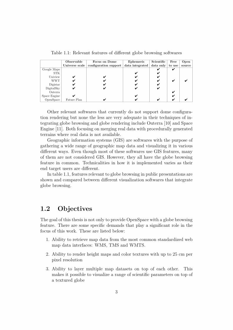
Table 1.1: Relevant features of different globe browsing softwares

Observable Focus on Dome Ephemeris Scientific Free Open

Universe scale configuration support data integrated data only to use source

Google Maps ✔ ✔

STK ✔ ✔

Uniview ✔ ✔ ✔ ✔

WWT ✔ ✔ ✔ ✔ ✔ ✔

Digistar ✔ ✔ ✔ ✔

DigitalSky ✔ ✔ ✔ ✔

Outerra ✔

Space Engine ✔ ✔ ✔

OpenSpace Future Plan ✔ ✔ ✔ ✔ ✔

Other relevant softwares that currently do not support dome configura-tion rendering but none the less are very adequate in their techniques of in-tegrating globe browsing and globe rendering include Outerra [10] and SpaceEngine [11]. Both focusing on merging real data with procedurally generatedterrains where real data is not available.

Geographic information systems (GIS) are softwares with the purpose ofgathering a wide range of geographic map data and visualizing it in variousdifferent ways. Even though most of these softwares use GIS features, manyof them are not considered GIS. However, they all have the globe browsingfeature in common. Technicalities in how it is implemented varies as theirend target users are different.

In table 1.1, features relevant to globe browsing in public presentations areshown and compared between different visualization softwares that integrateglobe browsing.

1.2 Objectives

The goal of this thesis is not only to provide OpenSpace with a globe browsingfeature. There are some specific demands that play a significant role in thefocus of this work. These are listed below:

1. Ability to retrieve map data from the most common standardized webmap data interfaces: WMS, TMS and WMTS.

2. Ability to render height maps and color textures with up to 25 cm perpixel resolution

3. Ability to layer multiple map datasets on top of each other. Thismakes it possible to visualize a range of scientific parameters on top ofa textured globe

3

4. Globe browsing should be done at interactive frame rates: at least 60frames per second on modern consumer gaming graphics cards

5. Correct positional mapping of objects rendered near the globe surface

6. Support animation of map datasets with time resolution

7. An intuitive interaction mode is also required to get the most out ofglobe browsing. It must support:

(a) Horizontal following of reference ellipsoid

(b) Decrease in sensitivity when closer to the surface of the globe

(c) Terrain following to avoid popping down under the surface

1.3 Delimitations

To focus on the important aspects of globe browsing and its purposes forpublic presentations, some important delimitations had to be taken into con-sideration.

We do not consider rendering of globes with distances to the origin greaterthan the radius of our solar system. Direct imaging of exoplanets is far fromusable for mapping and is mainly a method for locating planets [12]. Since wedon’t yet have map data for exoplanets, and OpenSpace does not currentlyaim at producing procedurally generated content, visualization of exoplanetsis not the focus for this thesis.

One important delimitation for the project is to limit the geometry of aglobe to height mapped grids. This will make it possible to perform vertexblending on the GPU as well as simplify the implementation to a uniformmethod of rendering across the whole globe.

We will not focus on re-projecting maps between different georeferencedcoordinate systems. Therefore the implementation must be limited to readinga specific map projection. Reprojecting maps can be considered future workto generalize the ability to read map data as well as optimizing renderingoutput and performance.

One goal of OpenSpace is to produce awe inspiring visual effects. Thecurrent state of the project requires the foundations to be in place and globebrowsing is one of the main features that need to be implemented before realsophisticated rendering techniques can be developed. We will not considerrendering of atmospheres or water effects and we will not consider shad-ing techniques that requires changing of the current rendering pipeline ofOpenSpace such as deferred shading.

4

1.4 Challenges

There are multiple technical challenges to tackle when designing a virtualglobe renderer. Cozzi and Ring [2] define the main challenges as following:

• Precision - In order to render small scale details of a virtual globe andalso dolly out to see multiple virtual globes within the solar system,the limited precision of computer arithmetics needs to be considered.

• Accuracy - Modeling globes as spheres is usually not a very accurateapproach, as many planets and moons that rotate have different polarand equatorial radii.

• Curvature - The curved nature of globes implies some extra chal-lenges as opposed to worlds modeled based on flat surfaces. The chal-lenge includes finding a suitable 2D-parameterization for tessellationand mapping.

• Massive datasets - It is usual for real world geographical datasetsto be too large to fit in GPU memory, RAM and even local drives.Instead, data need to be fetched from remote servers on demand usinga so called out-of-core approach to rendering.

• Multithreading - The need for multithreading is necessary as the pro-gram needs to retrieve geographical data from multiple sources, whileat the same time retain a steady frame rate for rendering.

Details in issues and proposed solutions to these challenges will be dis-cussed throughout the thesis.

5

Chapter 2

Theoretical Background

A sophisticated globe rendering system needs to rely on some theoreticalfoundations and algorithms developed for globe rendering. These founda-tions work as a base for the research performed for the thesis and the imple-mentation. The research is based on the proposed challenges.

2.1 Large Scale Map Datasets

Global maps with high level of detail can easily become too large to bestored and read locally on a single machine. A common way of storing largemaps is by representing them using several overviews. An overview is amap representing the same geographical area as the original map but downsampled by a factor of two just like a lower level of a mip map texture. Figure2.1 shows how the size of the maps in raster coordinates decreases with theoverview number.

...Overview: 0 1 n

y

x

y

2

x2

y

2n

x2n

Figure 2.1: The size of the map is decreasing exponentially with the overview.Figure adapted from [13]

The physical disk space of large global map datasets is often measuredin terabytes or even petabytes. In order to deal with such large datasets,web based services allow clients to specify parts of the map to download ata time. This is an important aspect in the out-of-core rendering required forglobe visualization.

6

2.1.1 Web Map Services

To standardize web requests for map data, the Open GIS Consortium (OGC)specified a web map service interface [14] and from that, specifications of sev-eral other map service interfaces have followed. The most common standardsare Web Map Service (WMS), Tile Map Service (TMS) and Web Map TileService (WMTS). Some other, more specific, examples of WMS-like servicesare WorldWind, VirtualEarth and AGS.

WMS

The WMS interface instructs the map server to produce maps as image fileswith well defined geographic and dimensional parameters. The image files canhave different format and compression depending on the provider. A WMSserver has the ability to dynamically produce map patches of arbitrary sizewhich puts some load on the server side [14]. The basic elements supportedby all WMS providers are the GetCapabilities and the GetMap operations.GetCapabilities gives information about the available maps on the server andtheir corresponding georeferenced metadata. The GetMap operation returnsthe map or a part of the map as an image file.

WMS requests are done using HTTP GET where the standardized requestparameters are provided as query parameters in the URL [14]. For example,setting the query parameter BBOX=-180,-90,180,90 specifies the size of themap in georeferenced coordinates while the parameters WIDTH and HEIGHT

specify the size of the requested image in raster coordinates. All name andvalue pairs for the GetMap request are defined under the OpenGIS Web MapServer Implementation Specification [14].

TMS

Tile Map Service (TMS) was developed by the Open Source Geospatial Foun-dation (OSGeo) as a simpler solution to requesting maps from remote servers.The specification uses integer indexing for requesting specific precomputedmap tiles instead of letting the server spend time on producing maps of ar-bitrary dimensions. The TMS interface is similar to WMS but simpler andit does not support all the features of WMS [15].

WMTS

Web Map Tile Service (WMTS) is another standard by OGC that requirestiled requests. It supports many of the features of WMS but, similar toTMS, removes the load of image processing from the server side and instead

7

forces the client to handle combination and cutouts of patches if required.The standard specifies the GetCapabilities, GetTile and GetFeatureInfo oper-ations. These operations can be requested with different message encodingssuch as Key-Value Pairs, XML messages or XML messages embedded inSOAP envelopes [16].

Tiled WMS

Before the WMTS standard was developed, some servers had already em-barked on the tiled requests by limiting the valid bounding boxes to valuesthat only produce precomputed tiles. These services can be referred to asTiled WMS and are nothing more than specified WMS services where theserver limits the number of valid requests [16].

2.1.2 Georeferenced Image Formats

There are several different standards for handling image data used in GISsoftwares. Some common file formats with image data and/or georeferencedinformation that are used in the below mentioned imagery products are:

• GeoTIFF - TIFF image with the inclusion of georeferenced metadata

• IMG - Image file format with georeferenced metadata

• JPEG2000 - Georeferenced image format with lossy or lossless com-pression

• CUB - Georeferenced image file standard created by Integrated Soft-ware for Imagers and Spectrometers (ISIS)

2.1.3 Available Imagery Products

There are several organizations working on gathering GIS data that can bevisualized as flat 2D maps or projected on globes. Many of them providetheir map data through web map services. However, they are often definedin different formats and sometimes available only as downloadable imagefiles.

Earth

NASA Global Imagery Browse Services (GIBS) provides several global mapdatasets with information about Earth’s changing climate [17]. The twosatellites Aqua and Terra orbit the Earth and are continuously measuring

8

multi band quantities such as corrected reflectance and surface reflectancealong with a range of scientific parameters such as surface and water tem-peratures, ozone, carbon dioxide and more. Many of the GIBS datasets areupdated temporally so that changes can be seen over time. Map tiles arerequested through a TMS interface and a date and time parameter can beset to specify a map within a certain time range.

Environmental Systems Research Institute (ESRI) is the provider of thesoftware ArcGIS that lets their users create and publish map data throughdifferent types of web map services. There are a lot of free maps to use;not only for Earth but other globes are covered too. ESRI supports a webpublication interface where web maps can be searched and studied in anonline map viewer.

National Oceanic and Atmospheric Administration (NOAA) for the U.S.Department of Commerce gathers and provides weather data of the US thatare hosted through different web map services using the ArcGIS online [18]interface by ESRI.

Mars

The first global color images taken of Mars were by the two orbiters of theViking missions that launched in late 1975. NASA Ames worked on creatingthe Mars Digital Image Models (MDIM) by blending a mosaic of imagestaken by the orbiters. United States Geological Survey (USGS) providesdownloading of image files in CUB or JPEG2000 format. The maps are stillthe highest resolution global color maps of the planet [19].

NASA’s Mars Reconnaissance Orbiter (MRO) is a satellite that has beenorbiting Mars since 2006, gathering map data by taking pictures of the sur-face. The satellite has three cameras; the Mars Color Imager (MARCI) formapping out daily weather forecasts, the Context camera (CTX) for imagingterrain and the High Resolution Imaging Science Experiment (HiRISE) cam-era for mapping out smaller high resolution patches covering limited surfaceareas of interest. NASA enables downloading of local patches and digitalelevation models (DEMs) and grayscale images taken by the CTX [20] andthe HiRISE [21] cameras in IMG and GeoTIFF formats.

Moon

The Lunar Mapping Modeling Project (LMMP) is an initiative by NASAto gather and publish map data of the Moon from a vast range of lunarmissions. The Lunar Reconnaissance Orbiter (LRO) is a satellite orbitingthe moon and gathering map data for future landing missions. These maps

9

have been put together into global image mosaics as well as DEMs. Mostglobal maps from LMMP can be accessed via the “OnMoon” web interface[22].

2.2 Modeling Globes

We will discuss different proposed methods used for modeling and render-ing of globes. The globe can be modeled either as a sphere or an ellipsoidand there are different tessellation schemes for meshing the globe. The tes-sellation depends on a map projection and out-of-core rendering requires adynamic level of detail approach for rendering.

2.2.1 Globes as Ellipsoids

Planets, moons and asteroids are generally more accurately modeled as ellip-soids than as spheres. Planets are often stretched out along their equatorialaxes due to their rotation which causes the centripetal force to counter someof the gravitational force acting on the mass. This effect was proven in 1687by Isaac Newton in Principia Mathematica [23]. The rotation causes a self-gravitating fluid body in equilibrium to take the form of an oblate ellipsoid,otherwise known as a biaxial ellipsoid with one semimajor and one semiminoraxis. Globes can be modeled as triaxial ellipsoids for more accuracy when itcomes to smaller, more irregularly shaped objects. For example Phobos, oneof Mars’ two moons, is more accurately modeled as a triaxial ellipsoid withradii of 27× 22× 18 km [2].

The World Geodetic System 1984 (WGS84) standard defined by NationalGeospatial-Intelligence Agency (NGA) models the Earth as a biaxial ellip-soid with a semimajor axis of 6,378,137 meters and a semiminor axis of6,356,752.3142 meters [2]. This is what is known as a reference ellipsoid; amathematical description that approximates the geoid of the earth as closelyas possible. The WGS84 standard is widely used for GIS and plays an im-portant role in accurate placements of objects such as satellites or space-crafts with position coordinates relatively close to the Earth’s surface. Inthe WGS84 coordinate system, the x-axis points to the prime meridian, thez-axis points to the North pole and the y-axis completes the right handedcoordinate system, see figure 2.2.

10

Figure 2.2: The WGS84 coordinate system and globe. Figure adapted from[13]

2.2.2 Tessellating the Ellipsoid

Triangle models are still the most common way of modeling renderable ob-jects in 3D computer graphics softwares, even though other rendering tech-niques such as volumetric ray casting also can be considered for terrain ren-dering [2, p. 149].

A triangle mesh, or more generally a polygon mesh, is defined by a limitednumber of surface elements. This means that ellipsoids need to be approx-imated by some sort of tessellation or subdivision surface when modeled asa polygon mesh. There are several techniques for tessellating an ellipsoid.Some of them are covered in this section.

Geographic Grid Tessellation

Tessellating the ellipsoid using a geographic grid is a very straightforwardapproach. Ellipsoid vertex positions can be calculated using a transformfrom geographic coordinates to Cartesian model space coordinates [2, p. 25].Figure 2.3 shows three geographic grid tessellations of a sphere with constantnumber of latitudinal segments of 4, 8 and 16 respectively.

A common issue with geographic grids is something referred to as polarpinching. At both of the poles, segments will be pinched to one point whichleads to an increasing amount of segments per area. This in turn results inoversampling in textures as well as possible visual artifacts in shading dueto the very thin quads at the poles as well as possible performance penaltiesfor highly tessellated globes.

11

Figure 2.3: Geographic grid tessellation of a sphere with constant number oflatitudinal segments of 4, 8 and 16 respectively

Figure 2.4: Quadrilateralized spherical cube tessellation with 0, 1, 2 and 3subdivisions respectively

Quadrilateralized Spherical Cube Tessellation

Another common tessellation method for spheres which can be generalized toellipsoids is the quadrilateralized spherical cube tessellation. The standardapproach is to subdivide a cube centered in the origin and then normalizethe coordinates of all vertices to map them on a sphere. There are also othermore complicated schemes designed to work with specific map projections[24].

To model an ellipsoid from a sphere, the vertices can be linearly trans-formed with a scaling in the x, y and z directions individually. Figure 2.4shows a tessellated spherical cube of four different detail levels.

Hierarchical Triangular Mesh

The hierarchical triangular mesh (HTM) is a method of modeling the skydome as a sphere proposed by astronomers in the Sloan Digital Sky Survey[25]. Instead of uniformly dividing cube faces, an alternative option is tosubdivide a normalized octahedron by, in each subdivision step, split everytriangle into four new triangles, see figure 2.5.

12

Figure 2.5: Hierarchical triangular mesh tessellation of a sphere with 0, 1, 2and 3 subdivisions respectively

Figure 2.6: HEALPix tessellation of three different levels of detail

Hierarchical Equal Area IsoLatitude Pixelation

Hierarchical Equal Area IsoLatitude Pixelation (HEALPix) is a sphericaltessellation scheme with corresponding map projection. The base level of thetessellation is built up of twelve quads, similar to a rhombic dodecahedron,which each can be subdivided further. The tessellation in figure 2.6 showshow the vertices in the HEALPix tessellation leads to curvilinear quads.

Geographic Grid Tessellation With Polar Caps

In their description of the ellipsoidal clipmaps method, Dimitrijević andRančić introduces polar caps to avoid polar issues related to geographic grids[24]. The polar caps are simply used as a replacement of the problematic,oversampled regions around the poles. The caps can be modeled as gridsprojected onto the ellipsoid surface in their own georeferenced coordinatesystems. One obvious issue with polar caps is the edge problem that occursdue to the fact that the caps are defined as separate meshes with verticesthat do not coincide with the geographic vertices of the equatorial region, seefigure 2.7. Dimitrijević and Rančić solves the issue by using a type of edgeblending between the equatorial and polar segments [24]. Figure 2.7 showsa sphere tessellated with one equatorial region and two polar regions.

13

Figure 2.7: Geographic tessellation of a sphere with polar caps

2.2.3 2D Parameterisation for Map Projections

A map projection P defines a transformation from Cartesian model spacecoordinates to georeferenced (projected) coordinates, as in equation 2.1. Theinverse projection P −1 is used to find positions on the globe surface in modelspace given georeferenced coordinates as in equation 2.2.

(

st

)

georeferenced

= ~P (x, y, z), (2.1)

xyz

modelspace

= ~P −1(s, t), (2.2)

where x, y and z are the Cartesian coordinates of a point on the ellipsoidsurface. The parameters s and t are georeferenced coordinates defining allpositions on the globe. The georeferenced coordinates can have differentdefinition range depending on which projection is used. An example can beletting is s = φ ∈ [−90, 90] and t = θ ∈ [−180, 180] which are latitude andlongitude respectively for geographic projections.

The globally positive Gaussian curvature of any intrinsic ellipsoid sur-face makes it impossible to unproject it on a flat 2D surface without anydistortions. Since it is embedded in a 3D space, some distortions must beintroduced when unprojecting the surface. The distortion can differ depend-ing on the projection used. Equal-area projections preserve the size of aprojected area as ∂s∂t/∂s0∂t0 = 1, while conformal projections preserve theshape of projected objects as ∂s/∂t = 1; s0 and t0 are coordinates at thecenter of the projection with no distortion. No global projection can be botharea-preserving and conformal [24].

There are several possibilities for defining a coordinate transform for mapprojections. A common approach is to project the ellipsoid onto anothershape that allows for being flattened out without distortion, such as a cube,a cylinder or a plane. These types of shapes are known as developable shapesand have zero Gaussian curvature.

14

The choice of map projection is tied together with the choice of ellipsoidtessellation. This is because the map often needs to be tiled up when render-ing. Each tile has its local texture coordinate system which need to have asimple transform from the georeferenced coordinate system for texture sam-pling. If the tiles can be affinely transformed to the georeferenced coordinatesystem, texture sampling can be done on the fly; otherwise the georeferencedcoordinates need to be re-projected which may be computationally heavy orimpossible for real time applications.

The European Petroleum Survey Group (EPSG) [26] has defined severalstandards for map projections of the Earth. Many of these are mentionedwhen discussing the different projections.

Geographic Projections

Geographic projections are widely used standards for parameterization ofellipsoids. The ellipsoid is projected onto a cylinder which is then unrolledto form the 2D plane of the projected coordinates.

Geographic coordinates are defined with a latitude φ and a longitude θand works together with geographic tessellations of ellipsoids. A commonissue with geographic projections is oversampling around the poles, as men-tioned in section 2.2.2. At the poles, all longitudes will always map onto onepoint and the distortion increases with the absolute value of the latitude.Figure 2.8 shows an unprojected geographic map and how it wraps aroundthe globe.

Figure 2.8: Geographic map projection. Figure adapted from [13]

Geocentric projection The simplest geographic parameterization usesgeocentric coordinates. Here the latitude and longitude are defined as theangle between a vector from the origin to a point on the ellipsoid surface andthe xy− and xz−planes respectively.

15

Geodetic projection Another standard, well used in ellipsoid representa-tions makes use of so called geodetic coordinates. This variety of geographiccoordinate systems is defined by the normal of the surface of the ellipsoidwhere the longitudinal angle is the angle between the normal and the yx-plane.

Figure 2.9 shows the difference between geocentric latitudes along withdifference in surface normals.

x

z

~pn̂c

n̂d

φdφc

Figure 2.9: Difference between geocentric latitudes, φc and geodetic lati-tudes, φd for a point ~p on the surface of an ellipsoid. The figure also showsthe difference between geocentric and geodetic surface normals, n̂c and n̂d,respectively.

In the case of perfect spheres, geocentric and geodetic projections of anypoint will yield the same result.

Geodetic coordinates are among the most commonly used geo referencedcoordinate systems when mapping ellipsoids to two dimensions.

Cozzi and Ring describes the transform from geodetic coordinates in theellipsoid class [2, p. 25]. For the Earth, the most commonly used geodeticcoordinate space is defined in the EPSG:4326 standard where the WGS84ellipsoid is used [27].

Mercator Projection

The mercator projection is a cylindrical projection widely used for presentingglobal maps in unwrapped form. The mercator projection preserves the hor-izontal to vertical ratio for small objects on the map. Hence, the mercator isa conformal projection in contrast to the geocentric and geodetic projections,which results in a non unit value in the ratio between the longitudinal andlatitudinal differentials, see figure 2.10.

The mercator projection compensates for the longitudinal distortion byintroducing a latitudinal distortion as well. Due to the polar singularities

16

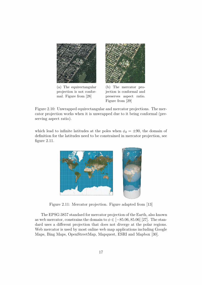
(a) The equirectangularprojection is not confor-mal. Figure from [28]

(b) The mercator pro-jection is conformal andpreserves aspect ratio.Figure from [29]

Figure 2.10: Unwrapped equirectangular and mercator projections. The mer-cator projection works when it is unwrapped due to it being conformal (pre-serving aspect ratio).

which lead to infinite latitudes at the poles when φd = ±90, the domain ofdefinition for the latitudes need to be constrained in mercator projection, seefigure 2.11.

Figure 2.11: Mercator projection. Figure adapted from [13]

The EPSG:3857 standard for mercator projection of the Earth, also knownas web mercator, constrains the domain to φ ∈ [−85.06, 85.06] [27]. The stan-dard uses a different projection that does not diverge at the polar regions.Web mercator is used by most online web map applications including GoogleMaps, Bing Maps, OpenStreetMap, Mapquest, ESRI and Mapbox [30].

17

Cube Map

Cube maps lack the polar singularities apparent in geographic parameteri-zations. The parameterized coordinates are often discretized to the six sidesof the cube, but they can also map directly to a global representation of anunwrapped cube, see figure 2.12.

Figure 2.12: Cube map projection. Figure adapted from [13]

Due to the traditions of map projections this is not a common formatused for map services so reprojection from a more common format is oftenrequired.

There are different cube map projections with different amount of area-and aspect distortions. Dimitrijević and Rančić mention and compares spher-ical cube, adjusted spherical cube, Outerra spherical cube and quadrilateral-ized spherical cube [24].

Tessellated Octahedral Adaptive Subdivision Transform

The Tessellated Octahedral Adaptive Subdivision Transform (TOAST) mapformat used in the globe browsing of Microsoft’s World Wide Telescope workstogether with the HTM tessellation [31]. Each triangular segment of theTOAST map maps to a triangle of a sphere that is tessellated as an octahe-dron and subdivided to form a sphere, see figure 2.13.

The TOAST format is just as the cube maps not a very well supportedformat for map providers and harder to use together with some of the mostcommon level of detail approaches due to the fact that most of them areoptimized for rectangular and not triangular map tiles.

Hierarchical Equal Area IsoLatitude Pixelation

The map projection that is used for the HEALPix tessellation is equal-area asthe name suggests. Figure 2.14 shows how the map wraps onto the sphere.

18

Figure 2.13: TOAST map projection. Figure adapted from [13]

The positive aspect about HEALPix compared to the TOAST format isthat the map is tiled into quads and not triangles which means that it isbetter suitable for the chunked LOD [2] algorithm. The map format is usedby NASA for mapping the cosmic microwave background radiation for theMicrowave Anisotropy Probe (MAP) [32], but is otherwise an uncommonformat when it comes to map services. That means that the maps need tobe re-projected from the more common formats for wider support.

Figure 2.14: HEALPix map projection. Figure adapted from [13]

Polar Projections

For parameterization of limited parts of the globe, such as the isolated poles,there are different projections to consider. Most common are different typesof azimuthal projections. These projections are defined by projecting allpoints of the map through a common intersection point and onto a flat sur-face. The Gnomonic projection maps all great circle segments (geodesics) tostraight lines by having the common intersection point in the center of theglobe.

Stereographic projections are defined when the common intersection pointis positioned on the surface of the globe on the opposite side of the poleto project. Polar stereographic projections are used to parameterize the

19

surface of the poles of the Earth. The standards EPSG:3413 and EPSG:3031define the stereographic projections for the North Pole and the South Polerespectively [27].

Dimitrijević and Rančić use another polar coordinate system to re-projectfrom geodetic coordinates in runtime. The transformation is a rotation of 90degrees around the global x−axis so that the resulting parametric coordinatesof the pole are given in their own geographic space with the meridian asequator. This projection is also known as the Cassini projection and it can beboth defined for spheres as well as generalized to ellipsoids. Polar projectionsare shown in figure 2.15.

(a) Cassini (b) Gnomonic (c) Stereographic

Figure 2.15: Polar map projections. Figure adapted from [13]

2.3 Dynamic Level of Detail

Dynamic level of detail (LOD) is an important part in handling the extensiveamount of data used in an out-of-core rendering software. The goal is tomaximize the visual information on screen while minimizing the workload.In their book 3D Engine Design for Virtual Globes, Cozzi and Ring describesLOD rendering algorithms by three typical steps: [2, p. 367]

1. Generation - Create versions at different level of detail of a model.

2. Selection - Choose a version based on some criteria or error metric (e.g.distance to object or the projected area it occupies on the screen).

3. Switching - Transition from one version to another in order to avoidnoticing of the change in LOD known as popping artifacts.

There are different types of LOD approaches for terrain rendering and asuitable approach should be chosen based on characteristics of the terrain.Terrains can for example be restricted to being represented as height maps -

20

Figure 2.16: A range of predefined meshes with increasing resolution. Dy-namic level of detail algorithms are used to choose the most suitable meshfor rendering

a characteristic that can be exploited by the rendering algorithm. Cozzi andRing describe the following three categories of LOD approaches: DiscreteLevel of Detail, Continuous Level of Detail and Hierarchical Level of Detail[2, p. 368-371].

2.3.1 Discrete Level of Detail

In the Discrete Level Of Detail (DLOD) approach, multiple different rep-resentations of the model are created at different resolutions. DLOD is ar-guably the most simple LOD algorithm. It works not only for digital terrainmodels, but for arbitrary meshes. The set of terrain representations caneither be predefined or generated using mesh simplification algorithms.

At run time, the main objective is to select one (or generate) a suitablerepresentation. This approach does not provide any means of dealing withlarge scale datasets which requires multiple levels of detail at the same time.This makes it unsuitable for globe rendering [2].

2.3.2 Continuous Level of Detail

The continuous LOD (CLOD) approach represents a model in a way thatallows the resolution to be selected arbitrarily. This is usually implementedby a base mesh combined with a sequence of operations that successivelychanges the level of detail of the model. Two typical such operations are“edge collapse” (removes two triangles from the mesh) and its inverse, “vertexsplit” (adds two triangles to the mesh). These operations are illustrated infigure 2.17.

According to Cozzi and Ring [2, p. 368] CLOD has previously beenthe most popular approach for rendering terrain at interactive rates, withimplementations such as Real-time Optimally Adaptive Mesh (ROAM) [33].The main reason CLOD algorithms are not widely employed these days is

21

V ertex Split −→←− Edge Collapse

Figure 2.17: Mesh operations in continous LOD

due to the increase in triangle throughput on modern GPUs, causing theCLOD operations done on the CPU in many cases to act as a bottleneck forthe rendering.

A special branch of CLOD worth mentioning is the so called infinite LOD.In this approach the terrain is represented by a mathematical function; animplicit surface. These functions can be defined by fractal algorithms andproduce complex characteristics or they can define simple geometric shapessuch as spheres or ellipsoids. As all points on these types of surfaces areprecisely defined, triangle meshes can be generated with no limit on the levelof detail. This approach is not suitable for incorporating real world data, butit is used by terrain engines such as Outerra and Terragen to procedurallygenerate terrain at any desired level of detail [34] [35].

2.3.3 Hierarchical Level of Detail

Hierarchical Level of Detail (HLOD) can be seen as a generalization of DLOD.HLOD algorithms operates on hierarchically arranged, predefined chunks ofthe full model. Each chunk is processed, stored and rendered separately. Bydoing this, HLOD approaches tackles the weaknesses of CLOD, essentiallyby doing the following:

1. Reducing processing time on CPU: The only CPU task that HLOD al-gorithms has to deal with during runtime is to select a suitable subsetof the predefined chunks for rendering. This is a relatively fast proce-dure in contrast to iteratively applying changes to the raw geometry,as done in CLOD.

2. Reducing data traffic to the GPU: Data is uploaded to the GPU inlarger batches but not very often, since the data is static and GPUcaching can be done. With CLOD, the geometry data is updated ona per-frame basis and can not be cached on the GPU. Being able toperform GPU caching allows HLOD to better minimize the traffic tothe GPU.

22

HLOD uses spatial hierarchical data structures such as binary trees,quadtrees or octrees for storing the chunk data. The root node of the treeholds a full representation of the model at its lowest level of detail in onesingle chunk. At successive levels, the model is represented at a higher levelof detail but divided up into several chunks. This concept is illustrated witha quad tree holding chunks representing a bunny model in figure 2.18.

Level 0

Level 1

Level 2

Figure 2.18: Bunny model chunked up using HLOD. Child nodes representhigher resolution representations of parts of the parent models

Generally, selecting all the chunks at a specific level in the tree yields acomplete representation of the model. Furthermore, chunks may be selectedfrom different levels for different parts of the model and still yield a fullrepresentation of the model. This allows for view dependent rendering of themodel. Algorithm 1 describes pseudo code for recursively rendering the fullmodel at view dependent level of detail.

RenderLOD (Camera C, ChunkNode N)

if ErrorMetric(C, N) < threshold thenRender(N , C)

else

for child in children(N) doRenderLOD(child, C)

end

end

Algorithm 1: Selecting chunks to render. The error metric depends onthe camera state and the chunk to render. A given chunk always has asmaller error metric than its parent.

23

This example uses a depth first approach for rendering of chunks. Othercommon schemes for traversing the hierarchy are breadth first and inversebreadth first.

The algorithm traverses the tree and calculates an error metric at eachnode with respect to the current camera position. If the calculated error islarger than a certain threshold, the algorithm recursively repeats the pro-cedure for all the chunk’s children, which have higher level of detail. Thisgeneral scheme can be used for rendering one-dimensional curves (using a bi-nary tree structure), two-dimensional surfaces (using a quadtree) or volumes(using an octree).

Another key feature of HLOD as opposed to DLOD and CLOD is thatit can naturally be integrated with out-of-core rendering, as chunks can beloaded into memory on-demand and deleted when not needed.

2.4 Level of Detail Algorithms for Globes

A number of different LOD algorithms has been introduced for the purposeof globe rendering. Two common algorithms used are Chunked LOD andGeometry Clipmaps, as pointed out by Cozzi and Ring [2].

2.4.1 Chunked LOD

The Chunked LOD method fits into the HLOD category and works by break-ing down the surface of the globe into a quadtree of chunks. There are severaldifferent ways of spatially organizing chunks and they depend on the tessel-lation of the globe.

Using a geographic grid tessellation, the chunks are in geographic spaceusing latitude φ and longitude θ coordinates. Figure 2.19 demonstrates thelayout of chunks as they are mapped in geographic coordinates onto an el-lipsoid representation of a globe.

(a) Chunk tree (b) Geodetic chunks (c) Globe

Figure 2.19: Chunked LOD for a globe

24

Chunks

Chunks should store the following data:

1. A mesh defining the terrain geometry (positions, normals, texture co-ordinates).

2. A monotonic geometric error based on the vertices distances to the fullydetailed mesh. The children of a chunk always have smaller geometricerror as they can better fit the highest level of detail model.

3. A known bounding volume encapsulating the mesh and all the chunk’schildren. This is used along with the geometric error metric whenselecting suitable chunks for rendering.

Depending on the implementation of the chunked LOD algorithm, theseproperties can be either calculated on the fly or preprocessed as suggested byCozzi and Ring [2, p. 447]. Furthermore, the chunk mesh must have definededges along its sides such that when two adjacent chunks are rendered nextto each other, there is no gap in between them.

Culling

An important thing to consider when dealing with chunks of a virtual globeis the fact that the chunks that are selected for rendering might not actuallybe visible on the screen. Needless to say, this is a waste of computationalpower and by eliminating these unnecessary draw calls, the performance ofthe globe renderer can be increased.

Camera frustum culling This is done by testing a bounding box of thechunk for intersection with the camera frustum. If the chunk is completelyoutside the frustum, the chunk can safely be culled as it will not be visiblein the rendered image. See figure 2.20a.

Horizon culling Even after camera frustum culling there are chunks thatstill do not contribute to the rendered image because they are positionedbehind the horizon. Figure 2.20b illustrates that most of a globe is actuallyinvisible to any observer. This can be used as a basis for culling some of theremaining chunks.

25

(a) Frustum culling (b) Horizon culling

Figure 2.20: Culling for chunked LOD. Red chunks can be culled due to thembeing invisible to the camera

Switching

Even when chunks can be selected in a way that guarantees a maximum pixelerror per vertex, the fact that full areas of multiple triangles are replaced allat once causes a drastic change in the rendered view. Even when the updatesare small per vertex, the update of whole chunk areas may be easily noticed.This is what is referred to as popping.

Minimizing popping artifacts is typically done by smoothly transitioningbetween levels over time. Cozzi and Ring suggest an approach, where alongwith each vertex, a delta offset is also stored [2, p. 451]. This delta offsetstores the difference between the chunk itself and the same region within theparent chunk. Using this difference, new vertices can be placed on alreadydefined edges and then interpolated into their actual positions. Figure 2.21illustrates the idea.

(a) An edge at a givenchunk level

(b) The same edge at thenext level

(c) The new vertex is in-terpolated into its trueplace

Figure 2.21: Vertex positions when switching between levels

The interpolation parameter can be based on the distance to the cameraor changed over time for each chunk.

26

Cracks and skirts

As chunks are tiled and rendered next to each other, it is desirable to makethe borders between chunks as unnoticeable as possible. Even though thechunk meshes are generated according to the requirements mentioned in theChunk subsection above, it is not possible to guarantee a watertight edgebetween two adjacent chunks of different LOD. Where adjacent chunks havedifferent detail level, so called T-junctions till emerge. These T-junctionscause cracks between the chunks as unwanted visual artifacts.

The easiest way to tackle this issue is not to try to remove the cracks,but instead try to hide them. The most common approach hides the cracksby simply adding an extra layer of vertices to the sides of sides of the mesh.This extra layer of vertices, which is also known as a skirt, is offset downvertically, as illustrated in figure 2.22.

By adding skirts to the chunk meshes, the model will not be renderedwith visible holes in it. Instead, the holes will be filled up with texturedtriangles.

(a) No skirts (b) Skirts

Figure 2.22: Chunks with skirts hide the undesired cracks between them

2.4.2 Geometry Clipmaps

A clipmap texture is a dynamic mip map where each image is clipped downto a constant size. This reduces the amount of memory of the whole textureto increase linearly instead of exponentially with the number of overlays forLOD textures [36]. Figure 2.23 a shows the difference between the amountof texture data stored in a regular mip map compared to a clip map.

The idea of clipmaps can be applied not only to textures but also to ge-ometries [36]. By representing a terrain by a stack of clipmap geometriesof different sizes, the resolution increases closer to the virtual camera, as il-lustrated in figure 2.24. As the view point moves around, the grids updatestheir vertex positions accordingly to keep the grid centered in the geometryclipmap stack. The position of each of the levels of the clip map geometries

27

Mip Map

Clip Map

Figure 2.23: Clip maps are smaller than mip maps as only parts of thecomplete map need to be stored. Figure adapted from [13]

snaps to a discrete coordinate grid with cell sizes equal to the distance be-tween two adjacent vertices. Due to the different grid resolution of differentlevels, the relative position of each sub grid must change so that they cansnap on a grid with higher level. This is illustrated with the dynamic interiorpart of the grid in figure 2.24.

Level 0

Level 1

Level 2

Level 3

Interior

View point

Figure 2.24: The Geometry Clipmaps follow the view point. Higher levelshave coarser grids but covers smaller areas. The interior part of the grid cancollapse so that higher level geometries can snap to their grid

Geometry clipmaps limits the terrain representation to be in the formof height maps. This is because the clipmap geometry moves around whenthe focus point changes and since the underlying terrain should not follow

28

the camera position, the clipmap geometries require vertex shader texturefetching. The texture coordinates are offset as the geometry clipmap movesto follow the focus point.

One of the main selling points for geometry clipmaps is the decrease inCPU workload and the increase in GPU triangle throughput [2]. There isno need to traverse a hierarchical structure such a quadtree. The number ofdraw calls will remain equal the number of clip maps instead of the number ofchunks which is often larger. The frame rate will also be relatively consistentif the number of layers in the clipmap stack remains constant [2].

2D Grid Geometry Clipmaps

Using geometry clipmaps to achieve dynamic level of detail for a heightmapped grid was proposed by Losasso and Hoppe [37]. The method islimited to rendering of equirectangular grids. When considering the ellip-soidal shape of a globe, the clipmap grid can be represented in geographiccoordinates mapped on an ellipsoid where the map texture coordinates inthe longitudinal direction wraps around the anti meridian. Rendering theclipmap close to the poles however will lead to polar pinching which breaksthe globe as illustrated in figure 2.25.

(a) Near the equator (b) Near a pole

Figure 2.25: Geometry Clipmaps on a geographic grid cause pinching aroundthe poles, which needs to be handled explicitly

Clipmap grids can also be used to model a spherical cube representationof a globe to avoid polar issues. This requires six clipmap partitions; one foreach side of the cube.

Spherical Clipmaps

Spherical clipmaps takes advantage of the fact that no observer will eversee more than half a globe at any time. The vertices of the clipmap aredescribed in polar coordinates with the center of the grid always following

29

Table 2.1: Comparison between geometry clipmaps and chunked LOD

Geometry Clipmaps Chunked LOD

Preprocessing Minimal ExtensiveMesh Flexibility None GoodTriangle Count High Lower

Ellipsoid Mapping Challenging StraightforwardError Control Poor Excellent

Frame-Rate Consistency Excellent PoorMesh Continuity Excellent Poor

Terrain Data Size Small LargeLegacy Hardware Support Poor Good

the camera position [38]. The coordinates of the vertices will therefore nothave any correspondence to texture coordinates which is why the algorithmis not widely adopted [24].

Ellipsoidal Clipmaps

Dimitrijević and Rančić introduces ellipsoidal clipmaps as a level of detailrendering method for globes [24]. It uses a geographic grid for the polarregions of the globe and solves the polar issues with the use of polar caps. Theadvantages compared to spherical cube clipmaps is that it uses the well knowngeographic map projection and reduces the number of geometry clipmappartitions from six to two. The globe is divided up into one equatorial regionand two polar regions. If the distance is close enough to the globe (3,000 kmabove the surface for the Earth), a maximum of two partitions is needed atany time [24].

The area distortion and the aspect distortion of the map projection ofthe ellipsoidal clipmap method is low compared to cube map projectionsbut requires extra care to hide the discontinuities that appear at the edgesbetween the equatorial and polar partitions [24].

The most generally used level of detail algorithms of today are chunkedLOD and varieties of geometry clipmaps. Cozzi and Ring compare the algo-rithms and gives the advantages and disadvantages depending on the needsof the globe browsing software. The main differences are summarized andpresented in Table 2.1 [2, p. 464].

30

2.5 Precision Issues

Modern graphics cards work with floating point variables and single precisionis the common standard [39]. With OpenGL 4.0 came the introduction ofdouble precision floating point numbers within the GLSL shader program-ming language [39]. The double precision floating point operations are sig-nificantly slower than their single precision counterparts [24]; we choose toavoid double precision floating point operations on the GPU for this reason.

In most computer graphics applications it is often sufficient to describepositional information in single precision floating point values. However,when simulating and visualizing the full scale of the universe and at thesame time globes with sub meter resolution, the issues of low precision floatoperations easily become predominant unless handled with care.

2.5.1 Floating Point Numbers

A floating point number y is represented by a sign bit s, a significand c ∈ N ,a base (also known as the radix) b ∈ Z, b > 2 and an exponent q ∈ Z. Seeequation 2.3.

y = (−1)s × c× bq (2.3)

These numbers are flexible since they can represent big ranges. Theyhave varying accuracy depending on the exponent q since the numbers c andq are stored as integers with a limited number of bits.

In the Institute of Electrical and Electronics Engineers 754 (IEEE 754)standard, the base b is a constant 2 or 10 and the significand c and theexponent q are set according to a well defined scheme [40]. With floating pointnumbers, operations such as addition and subtraction of values decreasesprecision due to a drop in the least significant bits [2]. The precision isreduced even more due to accumulating errors [2].

2.5.2 Single Precision Floating Point Numbers

A 32 bit floating point number can accurately represent around 7 significantdecimal figures in the IEEE 754 standard [2].

Considering an Earth sized globe with the origin in the center and aradius of 6× 106 meters, the theoretical vertical resolution is approximately6×106−7 = 0.6 meters. However, due to arithmetic operations the resolutionreduces even more. Furthermore, these issues get worse when consideringrendering of more objects in a scene that is representing not only one planetbut the entire solar system. The distance from the sun to the earth is roughly

31

1.5×1011 meters which leaves a positional resolution in the order of 1011−7 =104 meters which is far from acceptable when browsing globes.

2.5.3 Double Precision Floating Point Numbers

A double precision floating point number is able to accurately represent 16decimal figures [2]. Consider the Voyager 1 spacecraft, which left the solarsystem and entered interstellar space in August 25, 2012 and currently is ata distance in the order of magnitude of 1013 meters. This spacecraft is thefarthest any human made object has gone; farther away than all the planetsand can still be accurately positioned with sub meter resolution using doubleprecision floating point variables (of course assuming that the positional datais correct).

NASA’s Navigation and Ancillary Information Facility (NAIF) is the pro-ducer of the SPICE interface [5]. In SPICE, positional information of celestialbodies within our solar system are defined in double precision floating pointnumbers. Utilizing this precision makes it possible to accurately visualizespace crafts in relation to globes.

2.5.4 Rendering Artifacts

Vertex Position Jittering

One noticeable artifact related to the 32 bit floating point limitation of graph-ics cards is the discrete positioning of vertices when the origin is far awayfrom the rendered object. A clear example of this is shown in figure 2.26where Jupiter’s moon Europa is rendered with single precision floating pointoperations and the origin is placed at the barycenter of the solar system.

The artifact is shown as discrete positioning of vertices which causesjagged edges of the globe when the positions of the vertices exceeds sub-pixel precision. When moving the camera, the discrete positioning of thevertices appears to jitter due to the fact that they are transformed to cameraspace with limited precision.

Cozzi and Ring propose several different solutions to this problem whichinclude rendering “relative to center”, “CPU - relative to eye”, “GPU - rela-tive to eye” and “GPU - relative to eye - FUN90” [2].

Z-Fighting

Another well known issue related to precision in rendering of highly detailedobjects with a large range of possible distances to the camera is z-fighting. Z-fighting appears as triangles or fragments flipping between being positioned

32

Figure 2.26: Jupiter’s moon Europa rendered with single precision floatingpoint operations. The precision errors in the placement of the vertices isapparent as jagged edges even at a distance far from the globe.

in front of or behind each other. Normally the issue appears when it isundecidable what relative depth two objects have, see figure 2.27. Whendealing with large distances, undecidable depths can appear for objects suchas terrains with bigger relative depths.

Figure 2.27: Z-fighting as fragments flip between being behind or in front ofeach other

The problem is due to the inverse relationship that OpenGL implicitlyputs on the depth buffer when the perspective division is performed togetherwith the change in precision in the size of the floating point numbers. Thiscauses redundant precision close to the camera and increasingly lower preci-sion for coordinates with big depth values [2].

The problem is already handled in OpenSpace with the use of a lineardepth buffer. The depth buffer value is changed by explicitly setting thevalue of gl_FragDepth in all fragment shaders. The value is simply set tothe z-coordinate in camera space negated and normalized to fit all distanceswithin the observable Universe.

A negative aspect about setting the value of gl_FragDepth explicitlyis that early depth testing is not possible. This is OpenGL’s method ofdiscarding fragments before the fragment shader has been invoked. Not per-forming early depth testing leads to lower frame rates if the fragment shaderis heavy. Kemen discussed the implications of setting gl_FragDepth explic-

33

itly and concluded that for regular fragment processing, the change in framerate was not significant for the Outerra software [41].

Other previously proposed methods for handling depth buffer issues in-clude using multiple view frustums and complementary depth buffering [2].

2.6 Caching

Efficient caching of data is crucial in out-of-core, real time data visualiza-tion applications. Since the data sets dealt with often can be measured interabytes or petabytes, caching is most efficient if done in multiple stages.

2.6.1 Multi Stage Texture Caching

There are six levels of caching important to take into consideration for globerendering softwares. These are:

1. Local GPU texture memory

2. Local RAM

3. Local drive memory

4. Local server

5. Remote server

When implementing a globe rendering system, the local RAM memorycaching is of most interest and needs to be implemented explicitly.

2.6.2 Cache Replacement Policies

There are multiple different cache replacement policies, each used for differentpurposes. Some common policies are: First-In-First-Out, Last-In-First-Out,Least-Recently-Used, Most-Recently-Used, Least-Frequently-Used,Most-Frequently-Used.

When it comes to caching of texture tiles used for globe rendering, themost reasonable policy gets rid of the tiles that have not been used after asignificant amount of requests in favor of more recently used ones. Thereforethe Least-Recently-Used (LRU) cache replacement policy is typically used[2, p. 386].

34

LRU Caching

The LRU cache is filled up as new entries are requested. When the cache isfull, the least recently used entry will be thrown away when a new entry isto be added. This is implemented with a hash map and a doubly linked list.The hash map maps a unique resource identifier for an entry to a node inthe list, which in turn stores the entry. Every time an entry is accessed fromthe cache, the node storing that entry is placed first in the list. This schemeensures the least recently used entry will always be located in the back of thelist so that it can be thrown out when the cache is full, see figure 2.28.

→

Figure 2.28: Inserting an entry in a LRU cache.

35

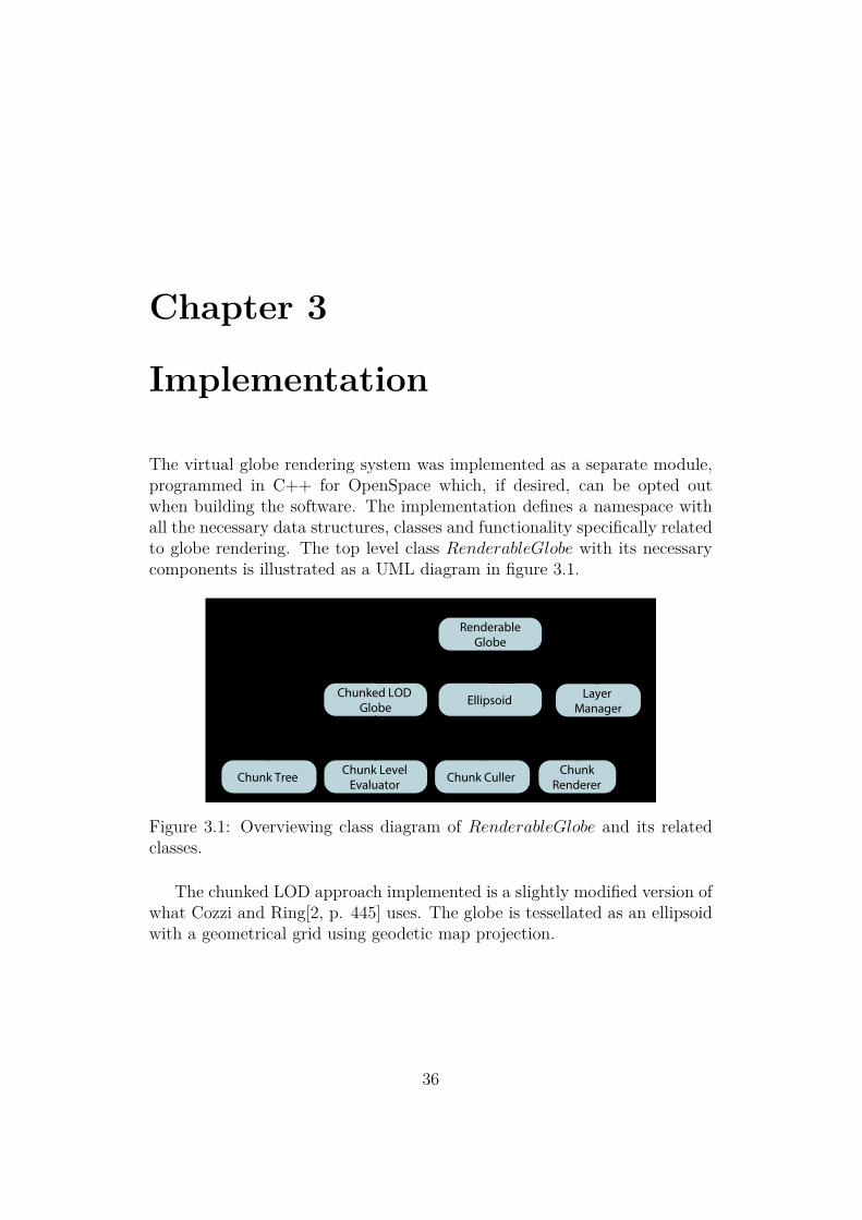
Chapter 3

Implementation

The virtual globe rendering system was implemented as a separate module,programmed in C++ for OpenSpace which, if desired, can be opted outwhen building the software. The implementation defines a namespace withall the necessary data structures, classes and functionality specifically relatedto globe rendering. The top level class RenderableGlobe with its necessarycomponents is illustrated as a UML diagram in figure 3.1.

Chunked LOD

Globe

Chunk Tree

Layer

Manager

Chunk

Renderer

Chunk Level

EvaluatorChunk Culler

0..m 0..m 1

1

1

1

Renderable

Globe

Ellipsoid

11

Figure 3.1: Overviewing class diagram of RenderableGlobe and its relatedclasses.

The chunked LOD approach implemented is a slightly modified version ofwhat Cozzi and Ring[2, p. 445] uses. The globe is tessellated as an ellipsoidwith a geometrical grid using geodetic map projection.

36

3.1 Reference Ellipsoid

The Ellipsoid class was implemented to handle all geographic related calcu-lations. These calculations include conversions between geodetic and Carte-sian coordinates and different kinds of projections onto the ellipsoid surface.These calculations are sped up by internal caching of a range of pre-calculatedvalues. Cozzi and Ring provide a complete reference on the implementation[2, p. 17].

The Ellipsoid uses several geographically related classes, which were usedin multiple places within the implementation. These are:

1. Angle - Handles angle related arithmetic, normalization and unit ab-straction (degrees and radians)

2. Geodetic2 - Represents a 2D geodetic coordinate (latitude, longitude)

3. Geodetic3 - Represents a 3D geodetic coordinate (latitude, longitude,altitude)

4. GeodeticPatch - Represents a rectangular region in geodetic space

3.2 Chunked LOD

The base of the chunked LOD algorithm revolves around the self updatingchunk tree. The chunk tree is a data structure built up of ChunkNodeswhich have the ability to split or merge dynamically. Besides storing fourChunkNode children and a reference to its ChunkedLodGlobe owner, eachChunkNode stores a Chunk.

3.2.1 Chunks

As opposed to the definition of chunks in the background section 2.4.1, thisimplementation of chunks is very lightweight - it does not store any textureor triangle mesh data. Instead, it stores the information needed to querytexture tiles from local in-memory caches. In the implementation suggestedby Cozzi and Ring, terrain triangle meshes are stored in each chunk. Inthe case of this implementation however, all terrain is rendered using heightmapped vertex grids. Thus there is no need for each chunk to store their ownvertex arrays. Instead they can simply share one single instance of a vertexgrid within a whole chunk tree. This means that vertices need to be offset byheight mapping on the GPU which makes it possibly to dynamically change

37

height datasets that does not require pre processing before they can be usedfor rendering.

The most important part of the chunked LOD algorithm is the ability todynamically select chunk nodes to split or merge. This is done by evaluatingall the leaf nodes of the chunk tree. Chunks that are cullable will indicatethat they can be merged by their chunk parent node. Chunks that cannotbe culled indicate whether they want be split or merged based on a chunkselection algorithm. If all child nodes to a common chunk parent indicatethey can be merged, the parent will merge its children. If any chunk reportsit want to be split, its chunk node will initialize four new children within thechunk tree.

3.2.2 Chunk Selection

The chunk tree is automatically reshaped depending on the virtual camera.Three different approaches for calculating the error metric were implemented.By letting the user dynamically adjust a LOD scale factor, performance canbe weighted against detail level.

By Distance

Letting the error depend on the distance between the closest point on thechunk and the camera d as in Equation 3.1, will lead to more or less constantsize of the chunks in screen space.

e = l − log2(s

d), (3.1)

where e is the error, l is the current level of the chunk, s is a LOD scalingfactor and d is the distance between the closest point of the chunk and thecamera. Using this distance as an error metric leads to bigger chunks fartherfrom the camera where less detail is needed.

By Projected Area

Another error metric is the area that the chunk takes up on the screen. Thebigger the area, the bigger the error.

The error must not be dependent of the direction of the camera. This isbecause a chunk rendered on a multi screen display, such as a dome, shouldnot have different errors between two or more screens which might lead todifferent levels and tearing between screens. Therefore the chunk is projectedon a unit sphere and not a view plane which would lead to view directiondependent error metrics.

38

Figure 3.2: Triangle with the area 1/8 of the chunk projected onto a unitsphere. The area is used to approximate the solid angle of the chunk used asan error metric when selecting chunks to render

The projected area is a solid angle approximated by extracting threepoints on the chunk and projecting them on a unit sphere centered in thecamera position. The three points define the closest of the four center trian-gles on the chunk, see figure 3.2. It is important that the triangle chosen forapproximating the projected area can never have two vertices on the sameupper or lower most edge. Such triangles (colored gray in figure 3.2) maycollapse down to a line and hence have zero area for chunks at the poles, thuscannot be used to approximate the area of the full chunk.

The actual approximated solid angle is the projected triangle area mul-tiplied by eight to accommodate a full chunk. This area is then subtractedby a constant value and scaled by a LOD scale factor to give similar LODscaling as the distance dependent chunk selection.

3.2.3 Chunk Tree Growth Limitation

The chunk selection algorithms described above determine a suitable level ofdetail based on the camera. This causes chunks that have too large of anerror to split. However, splitting a chunk will not result in higher level ofdetail unless the corresponding higher tile data (textures, heightmaps, etc)is also currently available for rendering. Therefore, the growth of the chunktree is limited by checking if there is any tile data there in the first place.This is useful in two scenarios:

1. Rendering of sparse map datasets which contain geographical regionswhere there are no data

2. Rendering of map datasets which are queried from remote servers; therewill always be some delay where the queried map data is not yet avail-able

39

By enabling limiting the chunk tree growth in these two scenarios, un-necessary chunk rendering calls can be avoided.

3.2.4 Chunk Culling

Given a chunk tree where the level of detail is selected based dynamicallybased on the camera, each chunk is then tested whether they are visible tothe camera. Chunks that are not visible are said to be “cullable”, and doesnot need to be rendered. The two chunk culling algorithms implemented areFrustum Culling and Horizon Culling. They both rely on - and have accessto - the minimum and maximum values of the chunk’s currently active heightmaps.

Frustum Culling

Frustum culling is implemented by first calculating a convex bounding poly-hedron for the chunk to be tested. The bounding volume is calculated onthe fly and takes into account any enabled height maps used to displace thevertices, making sure it fully encapsulates the displaced chunk vertices. Thepolyhedron is built up of eight vertices which are transformed to normalizeddevice coordinates (NDC) using the view-projection matrix of the camerafollowed by perspective division. Once in NDC, an axis aligned boundingbox (AABB) for the vertices is extracted. This AABB can then be testedagainst the screen bounds to determine if the chunk is outside the camera’sfield of view and thus is cullable. This is illustrated in figure 3.3.

ChunkModel space

Bounding polyhedronModel space

Bounding polyhedronNDC

Screen boundsNDC

AABBNDC

Inside? Yes:

Not cullable

Figure 3.3: Frustum culling algorithm. This chunk cannot be frustum culled.

Horizon Culling

Given a camera position, an object in position ~p with a bounding radiusr on the surface of the globe, it can be determined whether the object iscompletely hidden behind the globe’s horizon or not. The calculations aresimplified by approximating the globe as a sphere using the minimum radius

40

rg of its ellipsoid. Using the minimum radius and not a bigger number ensuresthat false occluding (chunks marked as invisible actually being visible) is notpossible [2, p. 393]. The minimum allowed distance l to the object can becalculated as the distance to the horizon lh added to the minimum alloweddistance to the object from the horizon lm. See figure 3.4. Once the minimumallowed distance is calculated it can be compared to the actual distance tothe object to determine if it is cullable or not.

lh

lm

rrg

~p

Figure 3.4: Horizon culling is performed by comparing the length lh +lm withthe actual distance between the camera position and the object at position~p.

When culling chunks, the closest position on the chunk is used as theposition ~p and the bounding height value as r.

3.3 Reading and Tiling Image Data

Fetching the right texture and preparing it for rendering onto chunks is afairly complicated process. Before digging into the details of this process,there are three concepts that need to be established, as they will be referredto throughout the description of the texture pipeline. These are:

1. TileIndex - A tuple of three integers (level, x, y) indexing a specificmap region on the globe.

2. TileStatus - An enumeration value indicating whether the Tile is“OK”, “Unavailable”, “Out of Range” or whether reading the pixeldata triggered an “IO Error”. Tiles that have the status “OK” areuploaded to the GPU and can be used for rendering.

41

3. RawTile - A texture carved out to fit the geographical region of aspecific chunk, along with meta data. Each RawTile is associated witha TileIndex and has a TileStatus. The RawTile class is guarantueedto be thread safe.

4. Tile - Like a RawTile, but the texture data is uploaded to the GPUand ready to use for rendering (unless it has a status not equal to“OK”). As opposed to RawTiles, the Tile class rely on an OpenGLcontext and thus is not thread safe.

All chunk height and texture data are represented using Tiles. Tilesare created on the client side (i.e. in OpenSpace) on the fly when they areneeded. As the pixel data may need to be read from disk or even requestedfrom remote servers, the whole tile preparation pipeline was implemented tobe executed on separate threads in order to avoid blocking of the renderingthread with image data reads.

During the iterative process of developing the texture tile pipeline, threelayers of abstraction were introduced in order to deal with the fairly highcomplexity. See table 3.1.

Table 3.1: Abstraction layers used in the texture data pipeline

Layer Component Responsibility Input –> Output

3 AsyncT ileDataset Async RawTile fetching TileIndex –> RawTile2 TileDataset Tiling, georeferencing, TileIndex –> RawTile

preprocessing1 GDAL Image formats, I/O Operations, pixel region –> pixel data

georeferencing

The subsequent sections of this chapter will cover each abstraction layerin more detail, starting from the bottom and going up the stack.

3.3.1 GDAL

Geospatial Data Abstraction Library (GDAL) is an open source library pro-viding a uniform interface for reading, manipulating and writing geospatialdata in the form of raster and vector data models [42]. It provides an in-terface allowing client code to specify pixel regions within a dataset to readfrom, independent of the underlying image format. Reading pixel data usingthe GDAL requires a set of parameters listed below and illustrated in figure3.5:

42

Figure 3.5: The required GDAL RasterIO parameters.

1. A map overview (also known as mip map) to read pixel data from

2. A pixel region within that map overview to read pixels from

3. The raster band(s) (e.g. color channels) to read

4. A pointer to sufficient user allocated memory where GDAL can writethe output of the read operation

5. The pixel region to write the output pixel data. The size of the pixeldata to be written may differ from the pixel region to read from, inwhich case GDAL will resample and interpolate the pixel data auto-matically

6. The layout (i.e. pixel spacing, raster band spacing and line spacing)

7. The data type to retrieve the pixel data in

With the given input parameters shown in figure 3.5, the resulting outputwould be the pixel data of the requested image region written with the pixellayout parameters to the provided memory block. The output is illustratedin figure 3.6.

0xabc123

256 px

212 px

Figure 3.6: Result of GDAL raster IO.

43

The same interface can also be used to read sparse datasets. A detailedexample of how to use GDAL for reading sparse datasets such as local, geo-referenced, image patches of high resolution can be founed in Appendix B.

GDAL also provides the coefficients of a geo-transform which defines themapping from raster coordinates to georeferenced coordinates. The geo-transform can be inverted to transform a georeferenced region to raster spacewhen specifying the area of an image tile to read.

3.3.2 Tile Dataset

TileDatasets carves out RawTiles from GDAL datasets based on aTileIndex. Along with the pixel data, the served RawTiles also containsome metadata. The metadata includes an error code if the read operationfailed and some basic information about to read pixel data, such as mini-mum and maximum pixel values. Figure 3.7 illustrates how the process fromTileIndex to RawTile is carried out. There are three gray subroutines; GetIO description, Read image data and Calculate metadata. These subroutinesare explained below.

Tile index

Tile index

Read image data

Pixel data

Raw tile

Calculate

metadata

Tile

metadataError

Raw tile

Tile dataset: Read tile data

Get IO description:

1. map overview

2. read/write regions

3. add padding

IO description

GDAL: Raster IO

Figure 3.7: The tile dataset pipeline takes a tile index as input, interfaceswith GDAL and returns a raw tile

44

Get IO Description

The IO description contains all tile specific information needed to performa map read request using GDAL. This includes the pixel region to read andwhere to store the result. The derivation of this information is summarizedin the following steps and illustrated in figure 3.8.

Figure 3.8: Overview of the calculation of an IO description.

1. Calculate a GeodeticPatch from TileIndex

2. Calculate the pixel coordinates for the patch in raster coordinate space

3. Calculate a suitable map overview

4. Transform pixel region to map overview pixel space

5. Add padding to the down scaled pixel region

6. Collect the information in an IO description object.

In the scheme in figure 3.8, step 1 is performed using equation 3.2,

φNE = 2πy/2level

θNE = 2πx/2level

side = 2π/2level,

(3.2)

where φNE and θNE are the latitude and the longitude of the north eastcorner of the tile and side is the side length of the tile.

Calculating the corresponding GDAL overview is done according to equa-tion 3.4,

Overview(level) = N − level − 1− log2(sizetile/sizemap), (3.3)

where level is given by the provided TileIndex, N is the total numberof overviews in the dataset, sizetile is a configurable constant defining the

45

preferred pixel size of a tile and sizemap is the size of the full map in pixels.The sizes can be either along the x− or y− axis. In the implementation thex−axis is used.

Pixel coordinates can easily be transformed across map overviews usingequation 3.4.

pn = pm × 2m−n (3.4)

Where n is the destination map overview and m is the source mapoverview. This is used for downscaling the pixel region in step 4, wheren is the calculated suitable overview and m is zero (i.e. the full map).

Padding is added to the pixel region in order to perform correct interpo-lation of pixel values across different tiles later during rendering. However,this may cause the pixel region to extend outside the map region. Thereforethe last finalize step also handles wrapping of the pixel region before return-ing the final IO description. The wrapping used is a CPU implementation ofGL_REPEAT .

Tile Meta Data

As mentioned, TileDatasets can be configured to calculate some metadataon the fly based on the pixel data that has been read. The metadata includesminimum and maximum pixel values within the pixel data and whether ornot the pixel data contains missing-data values. Having access to minimumand maximum values for height layer tiles is required for the culling to beperformed correctly since the cullers rely on having bounding boxes for thechunks. The meta data is collected by explicitly looping through all the pixelvalues on the client side.

Summary

To summarize, the implementation of TileDataset allow reading pixel datafrom a GDAL dataset corresponding to a specific TileIndex, along withmetadata unless opted out. The RawTiles that are served are padded inorder to perform smooth pixel blending between different tiles. RawTilesare not available for rendering since the data is not yet on the GPU.

3.3.3 Async Tile Dataset

AsyncT ileDatasets utilize a shared thread pool and own a TileDataset. Itdefines a concurrent job posting interface for concurrent reads within theTileDataset. It has two important functionalities: 1) enqueing tile read jobs

46

and 2) collect finished RawTiles. Reading RawTiles on separate threadsensures that the render thread will not be delayed by image data requests,see figure 3.9.

ThreadPool → Read from TileDataset

Tile dataset

Currently being

downloaded?Concurrent queue:

Append element

Figure 3.9: Asynchronous reading of Raw tiles can be performed on separatethreads. When the tile reading job is finished the raw tile will be appendedto a concurrent queue.

RawTileRawTile

Async ile dataset: Get raw iles

Figure 3.10: Retrieving finished RawTiles.

The AsyncT ileDataset internally keeps track of what tile indices it hasenqueued and what tile pixel regions are currently being read. If a pixelregion for a specific tile index is already enqueued or currently being read,the request is ignored. Figure 3.10 shows how raw tiles can be fetched oncethey are finished and enqueued.

47

3.4 Providing Tiles

Tiles have three properties: a texture, metadata and a status. The status isused to report any type of problem with the tile. Tiles that have the status“OK” are uploaded to the GPU and can be used for rendering.

Tiles are provided for rendering through TileProviders. They define aninterface that allow accessing tiles and meta data about the tiles. There aredifferent types of tile providers, but they must all implement the followingfunctionality:

• GetTile(TileIndex) - access the tile at the provided TileIndex

• GetDefaultTile() - returns a default Tile with status “OK”

• GetDepthTransform() - pixel value scale factor (for example convertingheight map values to meters)

• GetMaxLevel() - the maximum tile level supported by this provider)

• GetNoDataValue() - get value that should be interpreted as “no data”

• CheckTileStatus(TileIndex) - check TileStatus with no side effects

• Update() - called once per frame, allow for internal updates

• Reset() - full reset of internal state

Tile provider: Get tile

Tile index Tile

Figure 3.11: Tile provider interface for accessing tiles

The most important functionality is the GetTile ability, which is usedby client code to access the tiles. As tile providers may provide tiles of anystatus, the user of the tile provider is responsible to always check the statusof the requested tile before using the tile.

Several implementations of the tile provider interface were developed.They are all described below.

48

3.4.1 Caching Tile Provider

The CachingT ileProvider uses an AsyncT ileDataset to read RawTiles assoon as client code tries to access a specific tile. It internally polls theAsyncT ileDataset every update for finished raw tiles. The CachingT ileProviderconverts the raw tiles into tiles. This is done in the initialization step whichis part of the update method that is illustrated in figure 3.13. If no errors ofthe raw tile are reported, the tile gets the status “OK” and its texture datagets uploaded to the GPU. The tile also gets added to the in-memory “LeastRecently Used”-cache. The functionality of accessing tiles is illustrated infigure 3.12.

The uploading of texture data to the GPU needs to be on the renderingthread since there is where the OpenGL context resides. Tiles with datauploaded to texture memory will enable it for use in rendering of a chunk.

Figure 3.12: Tiles are either provided from cache or enqueued in an asyn-chronous tile dataset if it is not available

The functionality for internally updating the tile cache is illustrated infigure 3.13.

49

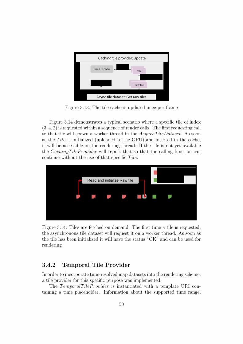
Caching tile provider: Update

Async tile dataset: Get raw tiles

RawTileRaw tile

Get raw tiles

TileTile

Initialize Tile

UpdateInsert in cache

Figure 3.13: The tile cache is updated once per frame

Figure 3.14 demonstrates a typical scenario where a specific tile of index(3, 4, 2) is requested within a sequence of render calls. The first requesting callto that tile will spawn a worker thread in the AsynchT ileDataset. As soonas the Tile is initialized (uploaded to the GPU) and inserted in the cache,it will be accessible on the rendering thread. If the tile is not yet availablethe CachingT ileProvider will report that so that the calling function cancontinue without the use of that specific Tile.

Time

Worker Thread

Main Thread

Initialize Tile

= Tile Unavailable

= Tile OK

getTile

( {3, 4

, 2} )

getTile

( {3, 4

, 2} )

getTile

( {3, 4

, 2} )

getTile

( {3, 4

, 2} )

getTile

( {3, 4

, 2} )

Read and initialize Raw tile

Figure 3.14: Tiles are fetched on demand. The first time a tile is requested,the asynchronous tile dataset will request it on a worker thread. As soon asthe tile has been initialized it will have the status “OK” and can be used forrendering

3.4.2 Temporal Tile Provider

In order to incorporate time-resolved map datasets into the rendering scheme,a tile provider for this specific purpose was implemented.

The TemporalT ileProvider is instantiated with a template URI con-taining a time placeholder. Information about the supported time range,

50

time resolution and expected timestamp format to be used in the templateURI is also passed during instantiation. In Listing 3.1, all tags starting withOpenSpace are used to configure information used to instantiate the temporaldataset. The tag GDAL_WMS contains a functional GDAL WMS dataset spec-ification. When requesting the URLs for the dataset, ${OpenSpaceTimeId}

will be replaced with the date and time in the specified format.

Listing 3.1: Temporal WMS dataset specification<OpenSpaceTemporalGDALDataset >

<OpenSpaceTimeStart >2015 -11 -24 </ OpenSpaceTimeStart >

<OpenSpaceTimeEnd ></ OpenSpaceTimeEnd >

<OpenSpaceTimeResolution >1d</ OpenSpaceTimeResolution >

<OpenSpaceTimeIdFormat >YYYY -MM -DD </ OpenSpaceTimeIdFormat >

<GDAL_WMS >

<Service name="TMS">

<ServerUrl >

http: // datasetURL /${ OpenSpaceTimeId }/${z}/${y}/${x}. jpg

</ ServerUrl >

</ Service >

...

</ GDAL_WMS >

</ OpenSpaceTemporalGDALDataset >

At runtime, the TemporalT ileProvider checks the global simulation time,quantizes that time with respect to the provided time resolution and lazilyinstantiates new CachingT ileProviders per timeframe within the temporaldataset. An schematic illustration is given in figure 3.15.

Temporal ile provider: Get ile

TileProviderTileProviderTileProviderCaching ile provider TileProviderTileProviderTileProviderCaching ile provider

2015-11-12 2016-06-01Current ime

Tile index Tile

TileTile

index

Figure 3.15: Each temporal snapshot is internally represented by a cachingtile provider

3.4.3 Single Image Tile Provider

This is a very simple implementation of the tile provider interface whichonly serves the same tile for every tile index. This tile provider was used for

51

testing and debugging alignment and padding between tiles, see figure 3.16.

Figure 3.16: Serving single tiles is useful for debugging chunk and texturealignment

3.4.4 Text Tile Provider

The ability to serve tiles with text rendered on the fly was implemented asa general debugging utility. The tiles are generated on demand by renderingtext to textures and cached using the same LRU caching mechanism as theCachingT ileProvider.

Tile

cached?

Figure 3.17: Serving tiles with custom text rendered on them can be used assize references or providing other information. The tile provider is internallyholding a LRU cache for initialized tiles

Two different types of TextT ileProviders were implemented.TileIndexT ileProvider serves tiles where each tile has its tile index renderedonto it and SizeReferenceT ileProvider uses the globe’s reference ellipsoidto render a size reference in meters or kilometers onto its tiles.

52

3.5 Mapping Tiles onto Chunks

In the implementation of chunks suggested by Cozzi and Ring [2], chunksstore the data they need for rendering by themselves. That means that assoon as a chunk has been fully initialized, it has everything it needs to berendered. However, when dealing with multiple map datasets potentiallyresiding on distant servers, there is no guarantee that all the tiles needed fora chunk to be rendered are available.

When an accessed Tile does not have the status “OK”, it can not beused for rendering. The second best thing to try is to check the parent of thetile. A parent tile is guaranteed to always cover a larger geodetic map regionthat includes its children’s subregions, but with lower number of pixels pergeodetic degree. Figure 3.18 demonstrates this with a simple example.

(a) Requested tile (b) Requested tile’s re-gion shown in its parenttile

Figure 3.18: Only the highlighted subset of the parent tile is used for ren-dering the chunk. Figure adapted from [13]

In figure 3.18, it is realized that in order to use a parent tile for rendering,the texture coordinates used to sample the parent tile needs to be adjustedto represent the same geographic region. This shows the need of a higherlevel concept than just Tiles, which leads to the introduction of ChunkT iles.

3.5.1 Chunk Tiles

A ChunkT ile represents a Tile that corresponds to a specific Chunk. Itstores a Tile which is guaranteed to have the status “OK” along with atransform defined by a scaling and translation component. The transform isused to map texture coordinates of the chunk into its corresponding geodeticregion within the tile.

53

The algorithm used for selecting the highest resolution ChunkT ile froma tile provider is described by the pseudo code in Listing 3.2.

Listing 3.2: Selecting optimal Chunk TilesChunkTile TileSelector :: getChunkTile ( TileProvider * tp , TileIndex ti){

TileUvTransform uvTransform ;

uvTransform . uvOffset = glm :: vec2 (0, 0);

uvTransform . uvScale = glm :: vec2 (1, 1);

while (ti. level > 1) {

Tile tile = tp -> getTile (ti);

if (tile. status == Tile :: Status :: OK) {

return { tile , uvTransform };

}

else {

ascendToParent (ti , uvTransform );

}

}

uvTransform . uvOffset = glm :: vec2 (0, 0);

uvTransform . uvScale = glm :: vec2 (1, 1);

return { tp -> getDefaultTile () , uvTransform };

}

The subroutine ascendToParent returns an updated transform whichmaps texture coordinates to the same geodetic region within the next parenttile. The routine is described in Listing 3.3.

Listing 3.3: Ascend to parentvoid TileSelector :: ascendToParent ( TileIndex & tileIndex , TileUvTransform &

uv) {

uv. uvOffset *= 0.5;

uv. uvScale *= 0.5;

if ( tileIndex . isEastChild ()) {

uv. uvOffset .x += 0.5;

}

// In OpenGL , positive y direction is up

if ( tileIndex . isNorthChild ()) {

uv. uvOffset .y += 0.5;

}

tileIndex . toParent ();

}

As opposed to regular tiles, chunk tiles can always be used for renderingsince they by definition always have the status “OK”.

3.5.2 Chunk Tile Pile

A ChunkT ileP ile represents a range of ChunkT iles across multiple mip lev-els. They contain the information needed to perform the LOD switching laterdescribed under section 3.7.5. Retrieving a ChunkT ileP ile simply requires

54

a tile index of the highest desired mip level (highest LOD) and the numberof desired ChunkT iles in the pile as described in Listing 3.4.

Listing 3.4: Instantiating a Chunk Tile PileChunkTilePile TileSelector :: getChunkTilePile ( TileProvider * tp , TileIndex

ti , int n){

ChunkTilePile chunkTilePile ;

for (int i = 0; i < n; ++i){

chunkTilePile . push_back ( getChunkTile (tp , ti));

ti. toParent ();

}

return chunkTilePile ;

}

As an example: Assuming that the texture data is available in localmemory, invoking the getChunkTilePile method with index {x : 2240, y :4824, level : 13} and a chunk tile pile size 3, would return the ChunkT ileP ilerepresented in figure 3.19.

(a) Tile (b) Parent 1 (c) Parent 2

Figure 3.19: The image data of a given chunk tile pile. Only the highlightedsubset of the parent tiles are used for rendering the chunk. Figure from [28]

As chunk tiles are guaranteed to be good for rendering on the GPU (sincetheir tiles are guaranteed to have the status “OK”), all ChunkT ileP iles areguaranteed to be good for rendering as well.

3.6 Managing Multiple Data Sources

The LayerManager maintains and organizes different types of texture datasources into groups. This is required as different types of texture datasets areused for different purposes and rendered in different ways. The LayerManagerowns seven LayerGroups; these are:

55

1. HeightLayers

2. ColorLayers

3. ColorOverlays

4. GrayScaleLayers

5. GrayScaleOverlays

6. NightLayers

7. WaterMasks

3.6.1 Layers

Much like in image editing softwares, a layer in this context represents araster of pixels, which among other internally ordered raster of pixels, areused to produce a final result. A Layer consists of three things:

1. A TileProvider - Used for accessing tiles of texture data.

2. A collection of render settings for real time image processing. The pa-rameters implemented at this stage are gamma, multiplier and opacity.

3. A simple boolean property which specifies whether the layer is enabledor disabled. Disabled layers are not used in rendering.

Layers allow for retrieving of ChunkT ileP iles, as described in section3.5.2. The class hierarchy and data flow is illustrated in figure 3.20.

3.6.2 Layers on the GPU

The data hierarchy defined by LayerManager can almost be reproduced onthe GPU by using GLSL in a near object-oriented approach. In order tohandle the data mapping between the CPU and GPU, a CPU representationof the GPU data hiearchy was implemented. This allows for easily updatingthe values of uniform variables and map uniform names to uniform locations.

56

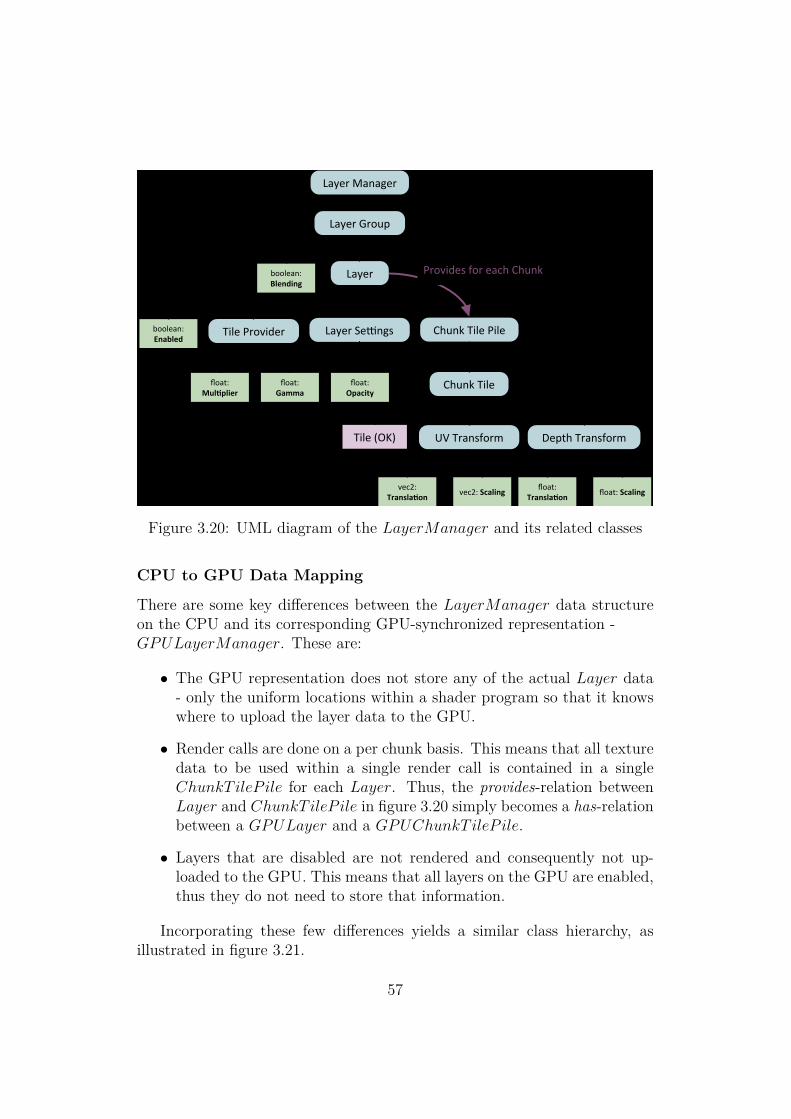
1

1 1 1

1

1 1 1 1

11

111

1

Tile (OK)

0..m

0..m

0..m

vec2:

Translaionvec2: Scaling

float: Translaion

float: Scaling

float: Gamma

float: Opacity

float: Muliplier

Layer Manager

Layer Group

Layer

Layer Seings Chunk Tile Pile

Chunk Tile

UV Transform Depth Transform

boolean: Blending

Tile Providerboolean: Enabled

Provides for each Chunk

Figure 3.20: UML diagram of the LayerManager and its related classes

CPU to GPU Data Mapping

There are some key differences between the LayerManager data structureon the CPU and its corresponding GPU-synchronized representation -GPULayerManager. These are:

• The GPU representation does not store any of the actual Layer data- only the uniform locations within a shader program so that it knowswhere to upload the layer data to the GPU.

• Render calls are done on a per chunk basis. This means that all texturedata to be used within a single render call is contained in a singleChunkT ileP ile for each Layer. Thus, the provides-relation betweenLayer and ChunkT ileP ile in figure 3.20 simply becomes a has-relationbetween a GPULayer and a GPUChunkT ileP ile.

• Layers that are disabled are not rendered and consequently not up-loaded to the GPU. This means that all layers on the GPU are enabled,thus they do not need to store that information.

Incorporating these few differences yields a similar class hierarchy, asillustrated in figure 3.21.

57

Figure 3.21: UML structure for corresponding GPU-mapped hierarchy. Theclass GPUData<T> maintains an OpenGL uniform location

58

The leaf classes within the class hierarchy store one uniform locationeach and represent one GLSL uniform value. The declaration of the layeruniforms within the shader code is defined so that it matches the exact samehierarchy. This is implemented by mapping C++ classes to GLSL structsand representing one-to-many relationships as structs with either a range ofconformally named fields or plain GLSL arrays.

Updating the GPU Data

With this 1:1 data mapping between the CPU and GPU, all the GPU-prefixedclasses were given two responsibilities.

1. Bind its uniform locations to GLSL variable names within a providedshader program

2. Set its uniform values within a provided shader program. That is, aGPUChunkT ile should be able to set its uniform values from a regularChunkT ile

The leaf classes automatically takes care of both binding its uniform lo-cation to specific GLSL variables and setting their uniform values. Thecompound GPU-prefixed classes (non leaf classes) more or less simply prop-agates the method calls to all its dependents. When binding an object to avariable name, the GLSL variable identifiers are built up successively duringthe propagation down to the leaf classes. GPULayer is used as an examplein Listing 3.5.

Listing 3.5: Bind a GPU Layer to a Layer on the CPUvoid GPULayer :: bind( ProgramObject * p, std :: string nameBase , int pileSize )

{

this -> gpuChunkTilePile .bind(p, nameBase + "pile.", pileSize )

this -> gpuRenderSettings .bind(p, nameBase + " settings .")

}

In Listing 3.5, it can be concluded that each layer in the GLSL code mustbe a struct with a member called “pile” and a member called “settings”. Anexample of a fully resolved identifier is:

" ColorLayers [0]. pile. chunkTile0 . tileUvTransform . scaling "

When setting the values, the GPU representation of the data is up-dated based on the currently available Layer data and the update is prop-agated down to all the leaf classes. This is exemplified using code from theGPULayer class defined in Listing 3.6.

59

Listing 3.6: Set all GPU Layer variables from a CPU LayerGPULayer :: setValue ( ProgramObject * p, Layer & l, TileIndex ti , int n){

ChunkTilePile chunkTilePile = l. getChunkTilePile (ti , n);

this -> gpuChunkTilePile . setValue (p, chunkTilePile );

this -> gpuRenderSettings . setValue (p, l. renderSettings ());

}

3.7 Chunk Rendering

Rendering of chunks uses both vertex and fragment shaders. As the globegeometry is always represented as height maps, the same vertex geometry -a uniform grid - is used as a basis for rendering all chunks.

3.7.1 Grid

The vertex grid used for rendering a chunk has square size. It is defined bythe number of segments N along its sides, which is used to build up a twodimensional array of vertex coordinates. These vertex coordinates can beused both for texture fetching and as interpolation parameters in an inversegeographic projection to place each vertex in 3D space. The grid also containsthe extra strip of vertices defining the skirt of the chunk. Figure 3.22 showshow a the skirt region have uv-coordinate values less than 0 or greater than1 in either the u or the v dimension.

0.0 1.0

0.0

1.0

u

v

1

2

3

N

1 2 3 N

Figure 3.22: Grid with skirts with a side of N = 4 segments. Green representsthe main area with texture coordinates ∈ [0, 1] and blue is the skirt of thegrid.

60

3.7.2 Vertex Pipeline

Rendering the grid includes performing displacement mapping of the verticesbased on active heightmaps as well as offsetting skirt vertices downwards.Two different methods for rendering the vertex grid were implemented. Thefirst method performs these operations in model space, whereas the secondone performs these operations in camera space.

Model Space Rendering

The vertices of the grid is transformed into geographic space on the GPUusing a transform derived from the chunk’s tile index. From geographicspace, an inverse projection transform is applied to place the vertices inthe Chunk’s Cartesian model space. From this space, the vertices are thendisplaced according to active height maps. This approach yields a limitedprecision of the vertices as they are defined relative to the center of the globe.However, it provides high accuracy as the vertices are positioned exactly onthe globe in geodetic coordinates. Figure 3.23 illustrates inverse projectiontransform.

xyz

= P −1(φ, θ)→

Figure 3.23: Model space rendering of chunks is performed with a mappingof vertices from geodetic coordinates to Cartesian coordinates.

Figure 3.24 shows the pipeline for rendering a chunk using the modelspace method.

Figure 3.24: Vertex pipeline for model space rendering. Variables on theCPU are defined in double precision and cast to single precision before beinguploaded to the GPU.

61

Camera Space Rendering

Camera space rendering is performed by transforming the corner points of thechunk to camera space using double precision arithmetics. Once in cameraspace, the points are cast to single precision and uploaded to the GPU.All the other vertices within the grid is then positioned on the GPU usingbilinear interpolation of the corner points in camera space. The bilinnearinterpolation means the grid will be rendered without curvature. However,having the points in camera space solves the proposed precision issues sincethe precision will increase when the points are closer to the camera. Thisconcept is illustrated in figure 3.25 where the vertex position vector precisionincreases as vertices are closer to the camera.

Figure 3.25: Interpolating vertex positions in camera space leads to high pre-cision in the representation of vertex positions close to the camera comparedto positions defined in model space.

Figure 3.26 shows a flowchart of the local vertex rendering pipeline.

Figure 3.26: Vertex pipeline for camera space rendering. Variables on theCPU are defined in double precision and cast to single precision before beinguploaded to the GPU

62

Combination

Both methods are used within the rendering system. Using the camera spacerendering with bilinear interpolation method instead of model space render-ing is done for chunks at level 10 and higher. This means that chunks witha latitudinal and longitudinal curvature of 360/210 ≃ 0.3516 degrees and lessare rendered as flat surfaces.

3.7.3 Fragment Pipeline

The purpose of layered texture rendering is to provide the user an ability totoggle different kinds of layers for rendering a chunk. For each fragment, thefinal color is calculated by using the active layer groups. This is done usingthe following step in the fragment shader which is the same for the cameraspace rendered chunks as it is for the model space rendered chunks:

1. For all ColorLayers: Sample RGB, apply layer settings and updatefragment RGBA using alpha blending

2. For all GrayscaleLayers: Sample the grayscale value R, apply layersettings and update fragment V in color space HSV using alpha blend-ing

3. For all GrayscaleOverlays: Sample grayscale value R and A, applylayer settings and update fragment RGBA using alpha blending

4. For all WaterMasks: Sample A, apply layer settings and add A as aspecularity component for the fragment

5. For all NightTextures: Sample RGB, apply layer settings and up-date fragment RGBA using alpha blending in shaded regions of theglobe

6. Perform shading by darkening shaded regions

7. Add simple atmosphere color to RGB

8. For all ColorOverlays: Sample RGBA, apply layer settings and up-date fragment RGBA using alpha blending

All of these steps are optional and can be toggled by activating or de-activating layers or specifying whether or not to perform shading or useatmosphere for rendering. Sampling the color from a layer group is done bylooping through all layers in that group, see Listing 3.7. Listing 3.8 and 3.9

63

shows how layer weights and texture transforms for chunk tile piles are usedfor sampling of the tile textures. Layer settings is performed for all rasterbands within all layers. The application of layer settings is shown in Listing3.10.

Listing 3.7: Setting color for a given layer group. Example using ColorLayers

# for i in 0..#{ lastLayerIndexColorLayers } {

vec4 colorSample = getTexVal ( ColorLayers [#{i}]. pile ,

levelWeights , uv);

colorSample = performLayerSettings ( colorSample ,

ColorLayers [#{i}]. settings );

color = blendOver (color , colorSample ); // Alpha blending

}

# endfor

Listing 3.8: Getting texture value by blending a chunk tile pilevec4 getTexVal ( ChunkTilePile chunkTilePile , LevelWeights w, vec2 uv){

return w.w1 * getTexVal ( chunkTilePile . chunkTile0 , uv) +

w.w2 * getTexVal ( chunkTilePile . chunkTile1 , uv) +

w.w3 * getTexVal ( chunkTilePile . chunkTile2 , uv);

}

Listing 3.9: Using texture transform and sampling a texturevec4 getTexVal ( ChunkTile chunkTile , vec2 tileUV ){

vec2 samplePosition = TileUVToTextureSamplePosition ( chunkTile , tileUV );

vec4 texVal = texture ( chunkTile . textureSampler , samplePosition );

return texVal ;

}

Listing 3.10: Perform layer settingsfloat performLayerSettings ( float currentValue , const LayerSettings

settings ) {

float newValue = currentValue ;

newValue = sign( newValue ) * pow(abs( newValue ), settings . gamma );

newValue = newValue * settings . multiplier ;

newValue = newValue * settings . opacity ;

return newValue ;

}

3.7.4 Dynamic Shader Programs

The ability to dynamically toggle layers with dynamic blending requires mul-tiple sampling of textures in the fragment shaders. To avoid unnecessary pro-cessing when not all layers are in use there is a need to dynamically recompilethe shader programs as layers are toggled. We use the GLSL preprocessorin the General Helpful Open Utility Library (GHOUL) [43] to preprocess allshader programs when the number of layers in use change.

64

Table 3.2: Data used for a layer group for preprocessing of layer shaderprograms

Layer Group Preprocessing Data

Number of layers: integerBlending enabled: boolean

Table 3.3: Data used for a renderable globe for preprocessing of layer shaderprograms

Layer Shader Preprocessing Data

0..* Preprocessing data: Layer Group Preprocessing Data0..* Key-value pairs: pair of strings

We define a layer shader program to be a GLSL program object usingvertex and fragment shading. Moreover, it fits the pipeline of rendering achunk with a specific number of layer groups and a varying number of layersfor each group.

To decide whether or not a layer shader program needs to be preprocessedand re-compiled, the relevant Layer Shader Preprocessing Data is saved forthe layer shader program and compared to the updated preprocessing datato determine if it has been changed by the user. Table 3.3 shows whatdata is needed to preprocess layer shader programs. Key-value pairs canbe used to set properties that are used on a per-globe basis. Examples areperformShading : true or false, useAtmosphere : true or false. Lettingthe preprocessor handle these properties avoids the need of uniform variableuploading and GLSL if-statements. The preprocessor also handles unrollingof for-loops which go through all layers in a group, see Listing 3.7.

3.7.5 LOD Switching

Instead of the time based switching routine proposed by Cozzi and Ring [2],we perform a distance based switching which works on a per fragment ba-sis for textures and on a per vertex basis for height maps. The method isimplemented in the vertex and fragment shaders and uses linear interpola-tion between levels. The blending technique uses the concept of Chunk TilePiles as seen in section 3.5.2. A Chunk Tile Pile contains three chunk tilesof different level to achieve level blending which is used to avoid poppingartifacts.

When rendering a specific fragment of a chunk, blending between up tothree chunk levels can be used as a part of the switching in the chunked LOD

65

algorithm. Assuming that the level of Tile 0 is equal to the level of the chunkto render and that Chunk Tile 1 and Chunk Tile 2 are 1 and 2 levels lowerrespectively, three level weights can be determined based on the distance tothe fragment to achieve smooth transitions between levels. The three levelweights are based on an interpolation parameter t as in Listing 3.11.

Listing 3.11: Calculate level weights for three chunk tiles using an interpo-lation parameter calculated based on the distance between the camera andthe fragment

LevelWeights getLevelWeights ( float t){ // level interpolation parameter

LevelWeights levelWeights ;

levelWeights .w1 = clamp (1 - t, 0 , 1);

levelWeights .w2 = clamp (t, 0 , 1) - clamp (t - 1, 0 , 1);

levelWeights .w3 = clamp (t - 1, 0 , 1);

return levelWeights ;

}

The interpolation parameter t is calculated using the distance to thecamera d and the current level of the chunk l as in equation 3.5.

t = l − log2(s

d), (3.5)

where s is a scale factor determining how much of the higher level tileto use in the blending. In the ideal case, the interpolation parameter shouldbe a value between 0 and 1. However, adjacent chunks can have a differencein level greater than 1 which in turn leads to interpolation parameters withlarger values. This is why it is not enough to use two Chunk Tiles per ChunkTile Pile to guarantee no popping. Popping can also occur if the LOD scalefactor s is small enough for adjacent chunks to have even bigger difference inlevel. Figure 3.27 shows how the interpolation parameter from the desiredlevel is used for blending between tiles of different level.

160 2 4 6 8 10 12 140

1

2

3

4

d = distance

t = 1

log2(s/d)level

(a) Blending disabled

0 2 4 6 8 10 12 14 160

1

2

3

4t = level - log2(s/d)

log2(s/d)level

1 - t

d = distance

(b) Blending enabled

Figure 3.27: Blending on a per fragment basis. The level interpolation pa-rameter t is used to calculate level weights w1 = 1 − t and w2 = t, in thiscase using two chunk tiles per chunk tile pile.

66

3.8 Interaction

An interaction mode specifically for globe browsing had to be implementedto deal with the vast scale differences and limitations of camera movementsrequired for browsing globes.

Representing the camera state as a three dimensional Cartesian vectorfor the position and a quaternion for the rotation made it possible to achieveinteraction solving the proposed objectives. Basic linear algebra was usedon vectors such as the geodetic normal of the globe in the camera positiongeodetically projected on the surface, camera position and direction as wellas the height offset of the terrain.

The horizontal movement interaction speed was set to be proportionalto the distance from the camera to the terrain surface. That way the usercan come in close and slowly hover across the detailed terrains as well asquickly moving from one continent to the other by increasing the height tothe surface.

The camera rotation quaternion can be decomposed in to two rotations;one directing the camera in the direction of the geodetic normal and onedirecting it in the remaining view direction with a given roll. This way it ispossible to both travel across the surface and keeping the horizon angle aswell as looking around at the spot.

The camera is always pushed up above the surface of the terrain to avoidpenetrating it. The minimum height given in meters can be set together withother parameters such as sensitivity and friction.

67

Chapter 4

Results

Two types of results are presented in this chapter: screenshots showing dif-ferent visual aspects of the system and benchmarks focusing on the achievedperformance.

4.1 Screenshots

Screenshots from the implemented system are presented and described ineach subsection below. Figure 4.1 shows the Earth shaded using a simpleimplementation of an atmosphere together with a daily image of surfacereflectance.

Figure 4.1: Shaded Earth rendered with NASA GIBS VIIRS daily image [17]

68

4.1.1 Height Mapping

Figure 4.2 shows the Earth rendered with a height dataset displacing thechunks’ vertices according to the geometric shape of the ground.

(a) The volcano Gunung Agung on Bali.

(b) Looking south from Mount Everest

Figure 4.2: Earth rendered with ESRI World Elevation 3D height map [44].Color layer: ESRI Imagery World 2D [28]

69

4.1.2 Water Masking

Figure 4.3 shows the Earth rendered with a water mask layer enhancingspecular contrasts between land and water.

(a) Sun’s specular reflection in the Amazon River.

(b) Sun’s specular reflection around Bali, Indonesia.

Figure 4.3: Shaded Earth using water mask texture. Color layer: ESRIImagery World 2D [28]

70

4.1.3 Night Layers

Figure 4.3 shows the Earth rendered with a night layer showing light fromcities, which is only rendered on the night side of the planet.

(a) Earth at night

(b) New Deli at night

Figure 4.4: Night layers are only rendered on the night side of the planet.Night layer: NASA GIBS VIIRS Earth at night [17]

71

4.1.4 Color Overlays

To demonstrate color overlays, the three examples of figure 4.5 show howdifferent tile providers produce references useful for debugging or locationing.

(a) Color Overlay: tile indices (b) Color Overlay: size reference

(c) Color Overlay: reference features and reference labels [17]

Figure 4.5: Earth rendered with different color overlays used for reference.Color layer: ESRI Imagery World 2D [28]

72

4.1.5 Grayscale Overlaying

In figure 4.6, the great canyon Valles Marineris on Mars is rendered with alow resolution color layer combined with a higher resolution grayscale overlay.

(a) Color layer: Viking MDIM [19] (b) Grayscale layer: CTX Mosaic

(c) CTX Mosaic HSV blended on top of Viking MDIM [19]

Figure 4.6: Valles Marineris, Mars with different layers

73

4.1.6 Local Patches

Figure 4.7 shows the approach of local DTM patches in West Candor Chasma.

(a) Local Patch: CTX DTM patch (b) CTX mosaic, CTX DTM patchand 25 cm per pixel DTM patch

(c) CTX mosaic, CTX DTM patch and HiRISE 25 cm per pixel DTMpatch closeup

Figure 4.7: Local DTM patches of West Candor Chasma, Valles Marineris,Mars. All figures use color layer: Viking MDIM [19] and height layer: MOLA[45].

74

4.1.7 Visualizing Scientific Parameters

Using the vast amount of datasets provided by NASA GIBS [17], severalscientific parameters measured by the Terra and Aqua satellites among otherscould be visualized as a result of layered texture rendering. Three examplesare shown in figure 4.8.

(a) Ozone (measured in streaks) (b) Land temperature

(c) Sea surface temperature

Figure 4.8: Visualization of scientific parameters on the globe. All thesedatasets are temporal and can be animated over time. Datasets from [17].

75

4.1.8 Visual Debugging: Bounding Volumes

Bounding polyhedra are calculated on the fly for each chunk, taking ontoconsideration any currently enabled height dataset. These bounding vol-umes are then used for by culling algorithms. Figure 4.9 shows how smaller,more planar chunks can be encapsulated more tightly than large chunks bypolyhedron shapes of eight vertices converging to rectangular blocks for highchunk levels.

(a) (b)

(c) (d)

Figure 4.9: Rendering the bounding polyhedra for chunks at Mars. Notehow the polyhedra start out as tetrahedra for the largest chunks in 4.9a andconverge to rectangular blocks as seen in 4.9d.

76

4.1.9 Visual Debugging: Camera Frustum

Figure 4.10 shows a camera frustum visualized and the affect of frustumculling on chunks together with the difference in skirt length between levels.

Figure 4.10: Chunks culled outside the view frustum. The skirt length ofthe chunks differ depending on the level. The figure also shows how somechunks are rendered in model space (green edges) and some in camera space(red edges).

77

4.2 Benchmarking

This section cover a range of benchmarks diagnosing the behavior and per-formance of the system. The specifications for the computer used for bench-marking is defined in table 4.1.

Table 4.1: Computer used for Benchmarking

Computer Model: MacBook Pro (15” early 2011)Processor: 2GHz Intel Core i7

RAM: 8 GB 1333MHz DDR3 RAMGraphics: AMD Radeon HD 6490M 256 MB

78

4.2.1 Top Down Views

The chunk rendering algorithm was evaluated for a top down view at differentdistances to the ground. The settings for the evaluation are presented inTable 4.2. The camera views for the evaluation points are shown in figure4.11 and the results are presented in figure 4.12.

Table 4.2: Globe rendering settings for top down view benchmark

Globe: EarthMap datasets: HeightLayers = [GCS_Elevation [44]]

ColorLayers = [ESRI Imagery World 2D [28]]LOD Scale factor: 10.0Chunk Selection: By distance

Culling: Frustum culling, Horizon cullingLevel blending: EnabledCamera View: Facing down, varying altitudes

(a) Earth (b) East America (c) New York City

(d) Manhattan (e) Central Park

Figure 4.11: Top down views of Earth at different altitudes

79

Earth East America NYC Manhattan Central Park0

20

40

60

80

100

120

140 ChunksLeaf chunksRendered chunksFrame time [ms]Globe render time [ms]

Figure 4.12: As the camera descends towards the ground looking straightdown, the chunk tree grows but the number of rendered chunks remainsrelatively constant due to culling.

80

4.2.2 Culling for Distance Based Chunk Selection

The two culling algorithms frustum culling and horizon culling were evalu-ated in combination with the distance based chunk selection algorithm. Thesettings used are provided in table 4.3. Figure 4.13 shows the camera viewevaluated. Figure 4.14 shows an overview of the rendered chunks with theresults shown in figure 4.15.

Table 4.3: Globe rendering settings for evaluation of culling with distancebased chunk selection

Globe: EarthMap datasets: HeightLayers = [GCS_Elevation [44]]

ColorLayers = [ESRI Imagery World 2D [28]]LOD Scale factor: 7.8Chunk Selection: By distance

Culling: Evaluated

Level blending: EnabledCamera View: Looking towards western horizon

Location: New York, New Jersey

Figure 4.13: Chunks yielded by the distance based chunk selection algorithm.Brooklyn, Manhattan and New Jersey is seen in the camera view.

81

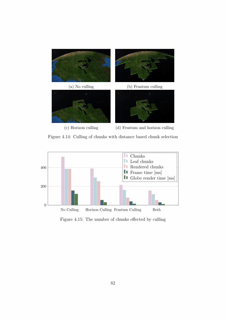
(a) No culling (b) Frustum culling

(c) Horizon culling (d) Frustum and horizon culling

Figure 4.14: Culling of chunks with distance based chunk selection

No Culling Horizon Culling Frustum Culling Both0

200

400

ChunksLeaf chunksRendered chunksFrame time [ms]Globe render time [ms]

Figure 4.15: The number of chunks effected by culling

82

4.2.3 Culling for Area Based Chunk Selection

The two culling algorithms frustum culling and horizon culling were evaluatedin combination with the area based chunk selection algorithm. The settingsused are provided in table 4.4. Figure 4.16 shows the camera view evaluated.Figure 4.17 shows an overview of the rendered chunks with the results shownin figure 4.18.

Table 4.4: Globe rendering Settings for evaluation of culling with area basedchunk selection

Globe: EarthMap datasets: HeightLayers = [GCS_Elevation [44]]

ColorLayers = [ESRI Imagery World 2D [28]]LOD Scale factor: 7.8Chunk Selection: By projected area

Culling: Evaluated

Level blending: EnabledCamera View: Looking towards western horizon

Location: New York, New Jersey

Figure 4.16: Chunks yielded by the projected area based chunk selectionalgorithm. Brooklyn, Manhattan and New Jersey is seen in the camera view.

83

(a) No culling (b) Frustum culling

(c) Horizon culling (d) Frustum and Horizon culling

Figure 4.17: Culling of chunks with area based chunk selection

No Culling Horizon Culling Frustum Culling Both0

100

200

ChunksLeaf chunksRendered chunksFrame time [ms]Globe render time [ms]

Figure 4.18: The number of chunks effected by culling

84

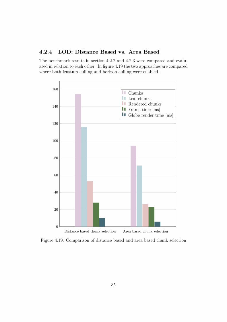
4.2.4 LOD: Distance Based vs. Area Based

The benchmark results in section 4.2.2 and 4.2.3 were compared and evalu-ated in relation to each other. In figure 4.19 the two approaches are comparedwhere both frustum culling and horizon culling were enabled.

Distance based chunk selection Area based chunk selection0

20

40

60

80

100

120

140

160ChunksLeaf chunksRendered chunksFrame time [ms]Globe render time [ms]

Figure 4.19: Comparison of distance based and area based chunk selection

85

4.2.5 Switching Using Level Blending

The visual result of using the distance based level blending is shown in figure4.20.

(a) Blending disabled (b) Blending enabled

Figure 4.20: Comparison of using level blending and no blending. Levelblending hides edges the underlying chunks

Table 4.5 shows the settings used to compare having level blending en-abled and disabled. To show the penalty in texture detail that is paid forusing level blending, the LOD scale factor was set low. Figure 4.21 showsthat the texture resolution becomes low enough to see the individual pixelswhen having a low LOD. The results in table 4.6 also show that figure 4.21acontains more visual information than 4.21b.

Table 4.5: Globe rendering settings used in benchmark

Globe: EarthMap datasets: HeightLayers = [GCS_Elevation [44]]

ColorLayers = [ESRI Imagery World 2D [28]]LOD Scale factor: 4.65Chunk Selection: By distance

Culling: Frustum culling, Horizon cullingCamera View: Horizon

86

(a) Blending disabled (b) Blending enabled

Figure 4.21: Comparison of level blending and no blending. The LOD scalefactor is set low to show the resolution penalty of using blending

Table 4.6: Level blending benchmarks. Comparing the disk space of a com-pressed JPG image of both cases works as a heuristic to the informationcontained in each image

Figure 4.21 No blending Level blending

Samples per fragment 1 3Mean globe render time 10.3 ms 10.1 ms

Mean frame time 40 ms 49 msScreenshot jpg size 1,1 MB 0,7 MB

87

4.2.6 Polar Pinching

The impact of polar pinching on the chunk tree was evaluated using bothdistance based chunk selection and area based chunk selection. The resultsare presented in figure 4.22.

Table 4.7: Globe rendering settings for evaluation of polar pinching

Globe: EarthMap datasets: HeightLayers = [GCS_Elevation[44]]

ColorLayers = [ESRI Imagery World 2D [28]]LOD Scale factor: 10.0Chunk Selection: Evaluated

Culling: Frustum culling, horizon cullingCamera View: Facing down

Location: Equator (at Quito, Ecuador) and North Pole

D: Equator D: Pole A: Equator A: Pole0

100

200

300

400

500 ChunksLeaf chunksRendered chunks

Render time [10−4 s]

Figure 4.22: Comparison of distance based and area based chunk selectionat the Equator and the North Pole. D = distance based, A = area based

88

4.2.7 Benchmark: Interactive Globe Browsing

The purpose of the globe browsing is to be able to interactively explore virtualglobes and map datasets. In order to capture how the system behaves overtime, a user interaction sequence was evaluated. The sequence is describedstep by step below and illustrated in Figure 4.23.

1. Camera views Earth from space

2. Descend down to Naturpark Karwendel, north of Innsbruck, Austria

3. Tilt camera up, view northern horizon

4. Turn camera 180 degrees, view southern horizon

5. Tilt camera down

Time [s]0 10 20 30 40 50 60 70 800

20

40

60

80

100

120

140

160

180

Chunk nodesLeaf chunk nodesRendered chunks

1. 2. 3. 4. 5.

Figure 4.23: Chunk tree over time when browsing the globe

89

4.2.8 Camera Space Rendering

Comparing the use of camera space rendering and model space rendering,vertex jittering is apparent when interacting close to the surface. Figure 4.24shows how vertex jittering is apparent when browsing a HiRISE patch closeto the surface of Mars. The visual result in the image is not as striking asthe artifact that appears when the camera is moving. Then the vertices arejittering only in the case of model space rendering and not for camera spacerendering.

(a) Camera space rendering (b) Model space rendering

Figure 4.24: Vertex jittering of model space rendering

90

Chapter 5

Discussion

In this chapter, the resulting implementation and design decisions madethroughout the research phase and development phase will be discussed alongwith the results presented in chapter 4.

5.1 Chunked LOD

The performance related results of the benchmarks presented in section 4.2are discussed below.

5.1.1 Chunk Culling

From Figure 4.11 and 4.23 it is noted that the chunk tree grows as the groundfacing camera comes closer to the surface, but the number of rendered chunksremain relatively constant. This is the desired result of the frustum cullingalgorithm, which efficiently culls most of the chunk tree as the camera looksstraight down towards the ground. In Figure 4.11 we can also see that thetotal globe rendering time does not only depend on the number of renderedchunks. Even though the render call done for each rendered chunk is quiteheavy (including accessing texture data and setting uniforms on the GPU),other things such as chunk selection and performing culling (done for eachleaf node) are operations that also affect the render time.

In figure 4.15, the culling algorithms are evaluated and compared fora camera view looking at the horizon. Looking at the horizon means amuch larger geographical area is visible to the camera compared to lookingstraight down towards the ground as in the case discussed above. This meansthat chunk culling algorithms can not be expected to increase the renderingperformance as much as in the case above. However, it can be seen that

91

by using both the culling approaches, the globe rendering time is reducedapproximately by a factor 10. When comparing the two, we see that thefrustum culling algorithm does a much better job reducing the number ofrendered chunks than than horizon culling. This is intuitively explained bythe fact that horizon culling can only cull chunks far away, where the selectionalgorithm prefers choosing a few big, low resolution chunks any way. Thefrustum culling algorithm, on the other hand, may cull chunks that are bothfar away and very close to the camera. However, there is no practical reasonfor not using both the algorithms in combination at any time. The overheadof running both algorithms is paid back in rendering time as seen in figure4.15.

5.1.2 Chunk Selection

In order to efficiently render camera views including facing the horizon, pa-rameter tuning and optimization should not focus on chunk culling.

Instead, the selection algorithm need to be carefully considered. In fig-ure 4.19, the two implemented chunk selection algorithms are compared toeach other for such a camera view. We see that the algorithm based on theprojected area is significantly faster than the distance based approach. Theexplanation for this is found by looking at the figures 4.13 and 4.16 show-ing the corresponding view for the distance based and projected area basedalgorithm respectively. The projected area based algorithm prioritize highlevel of detail close to the camera to a larger extent than the distance basedapproach, which is also how the algorithm gains its performance. By lookingat the closest rendered chunks however, we see that the same level of detailwas selected for both algorithms. Considering the relatively low difference inthe visual appearance, one conclusion is that the projected area based algo-rithm is an efficient way to select chunks for rendering, especially for cameraviews looking at the horizon. Visual penalties will mainly be apparent whenhigh detail is desired at distances far from the camera. Such cases can bewhen tall mountains are visible near the horizon.

5.1.3 Chunk Switching

The mipmapped texture data within a single dataset does not have to bestrictly down sampled versions of the original size. The dataset may becombined from multiple different data sources such as satellite imagery andaerial photographs. Thus, two adjacent mip levels within a map dataset maylook very different from one another. This is one motivation for using levelblending as a main approach for chunk switching.

92

As seen in the results of section 4.2.5, the level blending removes the oth-erwise visible edges between chunks of different level. However, the penaltyfor using level blending is not directly the increase in render time (whichis insignificant) but rather the loss of image quality, as seen in table 4.6.Enabling the level blending algorithm for this specific case reduces the JPGcompressed version of the screenshot from 1,1 Mb to 0,7 Mb; that is a re-duction of 37%. In other words, using level blending can be seen as tradeoff between poorer texture resolution versus popping artifacts and visibleedges. In the end it all boils down to a tradeoff in render time as the LODscale factor can be increased to compensate the overall loss in quality for therendered globe. The quality per rendered chunk, however, is undoubtedlyreduced notably.

As mentioned in section 5.1.2, the projected area based selection ap-proach was concluded to be more efficient than the distance based. However,using the area based approach comes with the drawback of not being able tocorrectly perform distance based chunk switching using level blending on aper-fragment basis. The convenience of using a simple distance based chunkselection algorithm is that the exact same calculations can be used in a frag-ment shader to calculate the interpolation parameter for the different miplevels of the texture datasets. Calculating a correct interpolation parame-ter corresponding to the projected area based chunk selection algorithm isa harder problem, not considered in the scope of this thesis. Conceptually,one approach could be to use bilinear interpolation based on four blendingcontrol points in each corner of the chunk. These values, however, wouldinherently depend on the LOD level of neighboring chunks, which makes theproblem non-trivial.

5.1.4 Inconsistent Globe Browsing Performance

Using quad trees (chunk trees) is a simple approach for hierarchically dividinga region into smaller subregions. However, the way the chunk trees arestructured may cause different geographical regions to correspond to differenttypes of chunk tree structures. That is, two different chunks on the samechunk level can correspond to large differences in the total number of nodesin the chunk tree. As an example: if the camera is looking at a small regionjust north of the equator, the whole southern hemisphere can be efficientlyculled. However, if the camera moves just a few meters south, the chunk treeneeds to suddenly consider a lot more chunks than previously. This effectwill cause the performance of the rendering system to be affected by location.This would explain the same number of chunk nodes in figure 4.12 for EastAmerica and New York.

93

From Figure 4.23 we can see that the chunk tree grows as the cameraviews the horizon, as do the number of rendered chunks. When turning thecamera 180 degrees, the chunk tree shrinks temporarily. This is explainedby the fact that the chunk tree growth is limited by the available tile data.Rotating half a revolution causes a lot of previously unseen chunks to nolonger be culled by the culling algorithms. The tree grows again as the maptiles for these chunks are being fetched.

5.2 Ellipsoids vs Spheres

Representing globes as ellipsoids and not as spheres was a decision settledearly in the development process. The accuracy that the ellipsoidal modelgives is important to be able to show near Earth orbits and rocket launcheswhere the space crafts need to be positioned accurately relative to the WGS84reference frame which is used in the SPICE library. Other globes such asthe planet Saturn has a clearly visible ellipsoidal shape due to its angularmomentum. This can now be shown in OpenSpace by configuring the planetto have the correct radii.

5.3 Tessellation and Projection

The choice of using geographic tessellation for the ellipsoid was a direct re-sult of using equirectangular geodetic map projections. The equirectangulargeodetic map projection is very common for many public map datasets andwas therefore a given choice to be able to visualize a vast amount of data onthe globes surfaces.

The drawbacks with oversampling at the poles giving undesired visualartifacts was considered, but in the end prioritized down due to time restric-tions. However, due to the fact that the issue of polar pinching was nothandled explicitly, the resulting issue of performance drops close to the polescan be seen in section 4.2.6.

The most reasonable solution to the polar issues would be to use polarcaps similar to Dimitrijević and Rančić’s solution [24]. Even though theLOD algorithm is different, the similarities in tessellation and map projec-tion would mean that the implementation would have similar characteristics.Polar caps will however not solve all problems related to poles in geograph-ical grid tessellations. The first time the software wants to render chunkson a polar cap near the pole, it will still need to request all the same tilesthat a it would using a standard geographical grid tessellation. If it later

94

is able to cache all reprojected tiles, they will be faster to render next timethey are requested. The requests together with the re-projections will makeit slower to visualize tiles at the caps, this could be a big limitation fordatasets that needs to be accessed fast such as temporal datasets used foranimating textures. Many of the GIBS datasets however are available inboth equirectangular format as well as polar stereographic (EPSG:3413) forthe North Pole and Antarctic polar stereographic (EPSG:3031) for the SouthPole. Hence re-projection would not be needed if the polar caps are definedwith stereographic projections.

5.4 Chunked LOD vs Ellipsoidal Clipmaps

Both Ellipsoidal clipmaps and chunked LOD were thoroughly considered asthe overall LOD algorithm to used. Both methods were implemented asproofs of concepts before deciding on using the chunked LOD approach.

The clipmap implementation was aborted as the chunked LOD was sig-nificantly more straight forward to implement and early on started yieldingvisible results. Moreover, having decided on using equirectangular tessella-tion and map projection, the ellipsoidal clipmap approach would completelydepend on an working implementation of polar caps, which would have ex-tended the implementation time further with the need of considering bothre-projection and edges.

Even though geometry clipmaps would pose some very different render-ing challenges than the chunked LOD approach, many components devel-oped for the chunked LOD approach could be shared between the two ap-proaches. The commonly used components would include the entire texturedata pipeline and layer structure along with all the geometric related calcu-lations, the interaction mode and various helper classes. The main differenceis the rendering pipeline even though it also has similarities; for example,using the model space and camera space vertex rendering schemes could bedone for geometry clipmaps just as well as for chunk grids.

5.5 Parallel Tile Requests

Requesting tiles from a given remote dataset could in theory be performedin parallel but GDAL puts some restrictions on open datasets. GDAL caninternally request tiles in parallel when performing the RasterIO operation.However, GDAL does not guarantee thread safe reading within all its formats.Reading from one open dataset on several threads in parallel often results

95

in corrupt tiles. If the parallelization is limited to be performed on separateoverviews however, GDAL’s data writing and caching would hopefully notlead to race conditions between threads since overviews are completely sep-arated from each other. Another method to speed up GDAL requests couldbe to open several GDAL dataset per tile dataset. However this will lead tointernal cache misses within GDAL that most likely results in even slowerrequests and unnecessary memory usage.

5.6 High Resolution Local Patches

The software was implemented to be able to handle highly detailed datasetsdown to 25 centimeters per pixel as shown in section 4.1.6 rendering HiRISEpatches. Using the combination of HiRISE patches, CTX patches and aglobal terrain model with textures, the detail level together with the vastscale of surrounding canyon walls resulted in a combined view as close aspossible to the real landscapes of Mars.

As described under appendix B however, reading local patches used torender in OpenSpace requires extensive amount of preprocessing. Anotherissue is that a very sparse dataset specified with a virtual dataset (describedin appendix B) currently poses on OpenSpace is that empty tiles outside ofthe defined region are still initialized which makes the software run slower.The preprocessing and the unnecessary initialization makes reading and ren-dering of local patches more of a proof of concept and will be left for furtherdevelopment as future work.

96

Chapter 6

Conclusions

From the results and experimentation of this globe rendering system, thefollowing conclusions have been drawn:

• Chunked LOD is the most straight forward approach for out-of-corerendering of large scale map datasets where accuracy is important.

• Using a combination of frustum culling and horizon culling, the ren-dering time can be kept relatively constant with respect to distance tothe ground when camera is facing straight down.

• A chunk selection algorithm based on the chunks projected area is moreefficient than one based on only the chunk’s distance to the camera.The projected area based approach is better in terms of resulting visualappeal versus rendering performance.

• Distance based level blending can be done on the fragment shader tosignificantly reduce the appearance of chunk edges successfully whenused in combination with distance based chunk selection. However,in order to perform accurate level blending using a area based chunkselection algorithm, another approach for the fragment shader must beconsidered.

• The number of chunk nodes in the tree depends not only on the chunkselection algorithm per se, but also on the geographic location of thecamera due to the underlying quad tree.

97

Chapter 7

Future Work

We will discuss the most relevant features that could be added to the globebrowsing module in the future. There are possibilities for optimizations aswell as a need for features, required from a fully versatile globe browsingsystem, that easily extends beyond the scope of this thesis.

7.1 Parallelizing GDAL Requests

Given the discussion about parallelizing of GDAL WMS requests under sec-tion 5.5, testing parallelizing on a per overview level would be reasonable tomaximize efficiency in tile requests. The best thing, of course, would be ifthe developers of GDAL made sure that WMS requests would be thread safe.

7.2 Browsing WMS Datasets Upon Request

The focus was not put on user interfacing, but instead the techniques requiredfor rendering. A given future feature however would be to provide the users ofthe software the ability to specify datasets to read during runtime. This couldbe done using the GetCapabilities operation for WMS or WMTS providersto be able to list all available datasets behind a service. Then users couldselect a specific dataset to load on demand.

7.3 Integrating Atmosphere Rendering

Integrating a sophisticated atmosphere rendering technique for globe brows-ing would make the complete experience more rewarding. Using atmospheric

98

parameters defining phenomena such as Rayleigh scattering and Mie scat-tering estimated for globes around our solar system, the representations ofother worlds would be more accurate. With the implemented system, theseestimations could be based on public, real world weather data. Atmospheresalso works great for generating depth cues which enhances the illusion of truescale within the visualization of globes.

7.4 Local Patches and Rover Terrains

The ability to read and render local patches will be developed further toensure easy integration of geographically smaller datasets. A goal in thefuture is to be able to read and render even higher resolution imagery thandemonstrated in this thesis. Rendering Mars rover terrain models, on top ofHiRISE patches, on top of CTX patches, on top of a global terrain datasetswould transport audiences and users of the software even closer to the realsurface of Mars with all the detail in imagery currently available throughresearch of the planet’s geology.

7.5 Other Features

There are other features that naturally can be incorporated to make thesoftware more usable.

A switching algorithm implemented on the shader corresponding to thearea based chunk selection algorithm can be researched and explored further.

Another switching approach than the level blending approach introducedcan be to temporally interpolate between levels as chunks are split. This willdecrease the number of textures needed for switching but will still lead tovisible edges between chunks of different levels.

The skirt lengths can be optimized to decrease the number of fragmentsrendered. This can be done if each chunk has knowledge of the adjacentchunks height data at the edges. To avoid potential cracks that might appearwhen a chunk of high level is adjacent to a chunk of low level, skirt lengthscan be set to be proportional to the geodetic size of the available height mapand not the chunk itself.

Annotations such as country names can currently only be rendered us-ing pixel based layers. Introducing vector formats for layers would make itpossible to display annotations such as text without the discrete changes ofdifferent levels.

Other types of tile providers can also be implemented. Examples are:

99

text tile provider for visualizing a lat-long grid, temporal tile provider usinglocal image data.

7.6 Other Uses of Chunked LOD Spheres in

Astro-Visualization

Rendering of ellipsoidal or spherical models is not only useful for globes.Being able to browse the night sky using an inverted sphere also requires aLOD approach to be able to visualize the most distant objects in high levelof detail. World Wide Telescope uses such a technique to render photographsof distant galaxies when pointing the camera to the sky. The edge of our ob-servable Universe could also be rendered as a sphere textured with a mappingof the cosmic microwave background radiation.

100

References

[1] OpenSpace,http://openspaceproject.com/, (accessed 2016-11-16)

[2] Patrick Cozzi and Kevin Ring, 3D Engine Design for Virtual Globes,CRC Press, 1st edition, 2011.http://www.virtualglobebook.com (accessed 2016-08-03)

[3] Google Maps,http://maps.google.se, (accessed 2016-08-17)

[4] National Oceanic and Atmospheric Administration, Science On aSphere,http://sos.noaa.gov/, (accessed 2016-08-17)

[5] NASA’s Navigation and Ancillary Information Facility, An Overview ofSPICE, NASA’s Ancillary Data System for Planetary Missions, 2016.http://naif.jpl.nasa.gov/pub/naif/toolkit_docs/Tutorials/

pdf/individual_docs/03_spice_overview.pdf, (accessed 2016-11-16)

[6] SCISS AB, Uniview,http://sciss.se/uniview, (accessed 2016-08-17)

[7] World Wide Telescope, American Astronomical Society,http://www.worldwidetelescope.org, (accessed 2016-08-17)

[8] Evans & Sutherland, Digistar,http://www.es.com/Digistar, (accessed 2016-08-17)

[9] Sky-Skan, DigitalSky,https://www.skyskan.com/products/ds, (accessed 2016-08-17)

[10] Brano Kemen and Laco Hrabcak, Outerra Website,http://www.outerra.com, (accessed 2016-08-17)

101

[11] Vladimir Romanyuk, Space Engine Website,http://en.spaceengine.org, (accessed 2016-08-17)

[12] Sasha Hinkley, Directly Imaging Exoplanets, Astrophysics Group,University of Exeter, 2016https://palereddot.org/directly-imaging-exoplanets/, (ac-cessed 2016-08-18)

[13] Map Projection Images,https://en.wikipedia.org/wiki/List_of_map_projections, (ac-cessed 2016-11-25)

[14] Open Geospatial Consortium Inc, OpenGIS Web Map Server Implemen-tation Specification, 2006.

[15] Open Source Geospatial Foundation, Tile Map Service Specification,https://wiki.osgeo.org/wiki/Tile_Map_Service_Specification,(accessed 2016-08-17)

[16] Open Geospatial Consortium Inc, OpenGIS Web Map Tile Service Im-plementation Standard, 2010.

[17] Global Imagery Browse Services GIBS Available Imagery Products,https://wiki.earthdata.nasa.gov/display/GIBS/GIBS+

Available+Imagery+Products, (accessed 2016-11-27)

[18] ESRI, Arcgis Online,https://www.arcgis.com, (accessed 2016-08-17)

[19] U.S. Geological Survey, Mars Viking MDIM21 ClrMosaic global 232m,http://astrogeology.usgs.gov/search/map/Mars/Viking/MDIM21/

Mars_Viking_MDIM21_ClrMosaic_global_232m, (accessed 2016-11-23)

[20] Online Map Viewer for MRO CTX Patches,http://viewer.mars.asu.edu/viewer/ctx#T=0, (accessed 2016-11-23)

[21] Lunar & Planetary Laboratory HiRISE Digital Terrain Models,http://www.uahirise.org//dtm/, (accessed 2016-11-23)

[22] NASA Jet Propulsion Laboratory, Onmoon Web Interface, CaliforniaInstitute of Technologyhttp://onmoon.jpl.nasa.gov, (accessed 2016-08-17)

102

[23] Isaac Newton, Philosophiae naturalis principia mathematica, J. Soci-etatis Regiae ac Typis J. Streater, University of California, 2011.https://books.google.se/books?id=-dVKAQAAIAAJ, (accessed 2016-11-11)

[24] Aleksandar M. Dimitrijević and Dejan D. Rančić Ellipsoidal Clipmaps -A planet-sized terrain rendering algorithm, In Proceedings of the EighthJoint Eurographics / IEEE VGTC conference on Visualization (EURO-VIS’06), Comput. Graph. 52, C (November 2015), 43-61, 2015.doi: http://dx.doi.org/10.1016/j.cag.2015.06.006, (accessed 2016-11-01)

[25] Hierarchical Triangular Mesh, Sloan Digital Sky Survey, 2007.http://www.skyserver.org/HTM/ (accessed 2016-11-12)

[26] European Petroleum Survey Group,http://www.epsg.org, (accessed 2016-11-11)

[27] Spatial reference list,http://spatialreference.org/ref/epsg/, (accessed 2016-08-10)

[28] ESRI, ArcGIS Online, ESRI Imagery World 2D WGS84,https://www.arcgis.com/home/item.html?id=

37b8a8b1014747deb5e15472d06d0da9, (accessed 2016-11-25)

[29] ESRI, ArcGIS Online, World Imagery,https://www.arcgis.com/home/item.html?id=

10df2279f9684e4a9f6a7f08febac2a9, (accessed 2016-11-25)

[30] Sarah E. Battersby, Michael P. Finn, E. Lynn Usery and, Kristina H.Yamamoto, Implications of Web Mercator and Its Use in Online Map-ping, Cartographica 49:2, 2014, pp. 85-101, 2014.doi: http://dx.doi.org/10.3138/carto.49.2.2313, (accessed 2016-11-11)

[31] Jonathan Fay, WorldWide Telescope Projection Reference,http://www.worldwidetelescope.org/docs/

worldwidetelescopeprojectionreference.html, (accessed 2016-11-16)

[32] NASA, Jet Propulsion Laboratory, HEALPix,http://healpix.jpl.nasa.gov/index.shtml, (accessed 2016-11-23)

[33] Mark Duchaineau, Murray Wolinsky, David E. Sigeti, Mark C. Miller,Charles Aldrich, and Mark B. Mineev-Weinstein. ROAMing Terrain:Real- Time Optimally Adapting Meshes, In Proceedings of the 8th

103

Conference on Visualization #97, pp. 81-88. Los Alamitos, CA: IEEEComputer Society, 1997,

[34] Brano Kemen, Procedural terrain algorithm visualization, 2009,http://outerra.blogspot.se/2009/02/

procedural-terrain-algorithm.html (accessed 2016-11-16)

[35] Terragen - Planetside Software, Terragen Wiki - Procedural Data, 2013,http://planetside.co.uk/wiki/index.php?title=Procedural_

Data, (accessed 2016-11-16)

[36] Christopher C. Tanner, Christopher J. Migdal, and Michael T. Jones,The clipmap: a virtual mipmap, In Proceedings of the 25th annual con-ference on Computer graphics and interactive techniques (SIGGRAPH’98), New York, NY, USA, 151-158, 1998.doi: http://dx.doi.org/10.1145/280814.280855, (accessed 2016-11-01)

[37] Frank Losasso and Hugues Hoppe Geometry Clipmaps: Terrain Render-ing Using Nested Regular Grids, ACM Trans. Graphics (SIGGRAPH),23(3), 2004.

[38] Malte Clasen and Hans-Christian Hege, Terrain rendering using spher-ical clipmaps, In Proceedings of the Eighth Joint Eurographics /IEEE VGTC conference on Visualization (EUROVIS’06), Aire-la-Ville,Switzerland, 2006.doi: http://dx.doi.org/10.2312/VisSym/EuroVis06/091-098, (accessed2016-11-16)

[39] Mark Segal and Kurt Akeley, The OpenGL Graphics System: A Speci-fication (Version 4.0 (Core Profile) - March 11, 2010), CRC Press, 1stedition, 2010.

[40] The Institute of Electrical and Electronics Engineers IEEE Standardfor Binary Floating-Point Arithmetic, The Institute of Electrical andElectronics Engineers, Inc, New York, 1985.http://ieeexplore.ieee.org/stamp/stamp.jsp?arnumber=30711,(accessed 2016-11-18)

[41] Brano Kemen, Maximizing Depth Buffer Range and Precision, Articlefor the Outerra software, 2012.http://outerra.blogspot.se/2012/11/

maximizing-depth-buffer-range-and.html (accessed 2016-11-14)

104

[42] The Open Source Geospatial Foundation, GDAL - Geospatial Data Ab-straction Library, GDAL Website,http://www.gdal.org, (accessed 2016-11-16)

[43] The General Helpful Open Utility Library,https://github.com/OpenSpace/Ghoul, (accessed 2016-11-23)

[44] Lucian Plesea ESRI World Elevation 3D Equirectangular Reprojection,http://198.102.45.23/arcgis/rest/services/worldelevation3d/

terrain3d?request=GetCapabilities, (accessed 2016-11-25)

[45] US Geological Survey Mars Orbiter Laser Altimeter (MOLA) DTM,http://astrogeology.usgs.gov/search/map/Mars/

GlobalSurveyor/MOLA/Mars_MGS_MOLA_DEM_mosaic_global_463m,(accessed 2016-12-12)

105

Appendices

106

Appendix A

General Use of Globe Browsing

in OpenSpace

https://github.com/OpenSpace/OpenSpace/wiki/

Concepts-Modules-GlobeBrowsing-GeneralUse

107

Appendix B

Build Local DEM Patches to

Load With OpenSpace

https://github.com/OpenSpace/OpenSpace/wiki/

Concepts-Modules-GlobeBrowsing-BuildLocalDEMPatchestoLoadWithOpenSpace

108