Deep Learning of Vortex Induced Vibrations

Maziar Raissi1, Zhicheng Wang2, Michael S. Triantafyllou2,and George Em Karniadakis1

1Division of Applied Mathematics, Brown University, Providence, RI, 02912, USA2Department of Mechanical Engineering, Massachusetts Institute of Technology,

Cambridge, MA 02139, USA

Abstract

Vortex induced vibrations of bluff bodies occur when the vortex sheddingfrequency is close to the natural frequency of the structure. Of interestis the prediction of the lift and drag forces on the structure given somelimited and scattered information on the velocity field. This is an inverseproblem that is not straightforward to solve using standard computationalfluid dynamics (CFD) methods, especially since no information is providedfor the pressure. An even greater challenge is to infer the lift and drag forcesgiven some dye or smoke visualizations of the flow field. Here we employdeep neural networks that are extended to encode the incompressible Navier-Stokes equations coupled with the structure’s dynamic motion equation. Inthe first case, given scattered data in space-time on the velocity field andthe structure’s motion, we use four coupled deep neural networks to infervery accurately the structural parameters, the entire time-dependent pressurefield (with no prior training data), and reconstruct the velocity vector fieldand the structure’s dynamic motion. In the second case, given scattereddata in space-time on a concentration field only, we use five coupled deepneural networks to infer very accurately the vector velocity field and allother quantities of interest as before. This new paradigm of inference in fluidmechanics for coupled multi-physics problems enables velocity and pressurequantification from flow snapshots in small subdomains and can be exploitedfor flow control applications and also for system identification.

Keywords: data-driven scientific computing, partial differential equations,physics informed machine learning, inverse problems, data assimilation

Preprint submitted to Journal Name August 29, 2018

arX

iv:1

808.

0895

2v1

[ph

ysic

s.fl

u-dy

n] 2

6 A

ug 2

018

1. Introduction

Fluid-structure interactions (FSI) are omnipresent in engineering appli-cations [1, 2], e.g. in long pipes carrying fluids, in heat exchangers, in windturbines, in gas turbines, in oil platforms and long risers for deep sea drilling.Vortex induced vibrations (VIV), in particular, are a special class of fluid-structure interactions (FSI), which involve a resonance condition. They arecaused in external flows past bluff bodies when the frequency of the shedvortices from the body is close to the natural frequency of the structure[3]. A prototypical example is flow past a circular cylinder that involves theso-called von Karman shedding with a non-dimensional frequency (Strouhalnumber) of about 0.2. If the cylinder is elastically mounted, its resultingmotion is caused by the lift force and the drag force in the crossflow andstreamwise directions, respectively, and can reach about 1D and 0.1D inamplitude, where D is the cylinder diameter. Clearly, for large structureslike a long riser in deep sea drilling, this is a very large periodic motion thatwill lead to fatigue and hence a short life time for the structure.

Using traditional computational fluid dynamics (CFD) methods we canpredict accurately VIV ([4]), both the flow field and the structure’s motion.However, CFD simulations are limited to relatively low Reynolds numbersand simple geometric configurations and involve the generation of elaborateand moving grids that may need to be updated frequently. Moreover, someof the structural characteristics, e.g. damping, are not readily available andhence separate experiments are required to obtain such quantities involvedin CFD modeling of FSI. Solving inverse coupled CFD problems, however,is typically computationally prohibitive and often requires the solution ofill-posed problems. For the vibrating cylinder problem, in particular, wemay have available data for the motion of the cylinder or some limited noisymeasurements of the velocity field in the wake or some flow visualizationsobtained by injecting dye upstream for liquid flows or smoke for air flows.Of interest is to determine the forces on the body that will determine thedynamic motion and possibly deformation of the body, and ultimately itsfatigue life for safety evaluations.

In this work, we take a different approach building on our previous workon physics informed deep learning [5, 6] and extending this concept to cou-pled multi-physics problems. Instead of solving the fluid mechanics equations

2

and the dynamic equation for the motion of the structure using numericaldiscretization, we learn the velocity and pressure fields and the structure’smotion using coupled deep neural networks with scattered data in space-timeas input. The governing equations are employed as part of the loss functionand play the role of regularization mechanisms. Hence, experimental inputthat may be noisy and at scattered spatio-temporal locations can be readilyutilized in this new framework. Moreover, as we have shown in previouswork, physics informed neural networks are particularly effective in solvinginverse and data assimilation problems in addition to leveraging and discov-ering the hidden physics of coupled multi-physics problems [7].

This work aims to demonstrate feasibility and accuracy of a new approachthat involves Navier-Stokes informed deep neural networks inference, and ispart of our ongoing development of physics-informed learning machines [5, 6].The first glimpses of promise for exploiting structured prior information toconstruct data-efficient and physics-informed learning machines have alreadybeen showcased in the recent studies of [8–10]. There, the authors employedGaussian process regression [11] to devise functional representations that aretailored to a given linear operator, and were able to accurately infer solu-tions and provide uncertainty estimates for several prototype problems inmathematical physics. Extensions to nonlinear problems were proposed insubsequent studies by Raissi et. al. [12, 13] in the context of both inferenceand systems identification. Despite the flexibility and mathematical eleganceof Gaussian processes in encoding prior information, the treatment of non-linear problems introduces two important limitations. First, in [12, 13] alocal linearization in time of the nonlinear terms in time is involved, thuslimiting the applicability of the proposed methods to discrete-time domainsand possibly compromising the accuracy of their predictions in strongly non-linear regimes. Secondly, the Bayesian nature of Gaussian process regressionrequires certain prior assumptions that may limit the representation capac-ity of the model and give rise to robustness/brittleness issues, especially fornonlinear problems [14], although this may be overcome by hybrid neuralnetworks/Gaussian process algorithms [15].

Physics informed deep learning [5–7] takes a different approach by em-ploying deep neural networks and leveraging their well known capability asuniversal function approximators [16]. In this setting, one can directly tacklenonlinear problems without the need for committing to any prior assump-

3

tions, linearization, or local time-stepping. Physics informed neural networksexploit recent developments in automatic differentiation [17] – one of the mostuseful but perhaps under-utilized techniques in scientific computing – to dif-ferentiate neural networks with respect to their input coordinates and modelparameters to leverage the underlying physics of the problem. Such neuralnetworks are constrained to respect any symmetries, invariances, or conser-vation principles originating from the physical laws that govern the observeddata, as modeled by general time-dependent and nonlinear partial differen-tial equations. This simple yet powerful construction allows us to tackle awide range of problems in computational science and introduces a potentiallytransformative technology leading to the development of new data-efficientand physics-informed learning machines, new classes of numerical solvers forpartial differential equations, as well as new data-driven approaches for modelinversion and systems identification.

Here, we should underline an important distinction between this line ofwork and existing approaches (see e.g., [18]) in the literature that elabo-rate on the use of machine learning in computational physics. The termphysics-informed machine learning has been also recently used by Wang et.al. [19] in the context of turbulence modeling. Other examples of ma-chine learning approaches for predictive modeling of physical systems in-clude [20–31]. All these approaches employ machine learning algorithmslike support vector machines, random forests, Gaussian processes, and feed-forward/convolutional/recurrent neural networks merely as black-box tools.As described above, our goal here is to open the black-box, understand themechanisms inside it, and utilize them to develop new methods and tools thatcould potentially lead to new machine learning models, novel regularizationprocedures, and efficient and robust inference techniques. To this end, theproposed work draws inspiration from the early contributions of Shekari Bei-dokhti and Malek [18], Psichogios and Ungar [32], Lagaris et. al. [33], aswell as the contemporary works of Kondor [34, 35], Hirn [36], and Mallat [37].

The focus of this paper is fluid-structure interactions (FSI) in general andvortex induced vibrations (VIV) in particular. Specifically, we are interestedin the prediction of the fluid’s lift and drag forces on the structure given somelimited and scattered information on the velocity field or simply snapshotsof dye visualization. This is a data assimilation problem that is notoriouslydifficult to solve using standard computational fluid dynamics (CFD) meth-

4

ods, especially since no initial conditions are specified for the algorithm, thetraining domain is small leading to the well-known numerical artifacts, andno information is provided for the pressure. An even greater challenge isto infer the lift and drag forces given some dye or smoke visualizations ofthe flow field. Here we employ Navier-Stokes informed deep neural networksthat are extended to encode the structure’s dynamic motion equation. Thepaper is organized as follows. In the next section, we give an overview ofthe proposed algorithm, set up the problem and describe the synthetic datathat we generate to test the performance of the method. In section 3, wepresent our results for three benchmark cases; (1) We start with a pedagog-ical example and assume that we know the forces acting on the body whileseeking to obtain the structure’s motion in addition to its properties with-out explicitly solving the equation for displacement. (2) We then considera case where we know the velocity field and the structural motion at somescattered data points in space-time. In this case, we try to infer the lift anddrag forces while learning the pressure field as well as the entire velocity fieldin addition to the structure’s dynamic motion. (3) We then consider an evenmore interesting case where we only assume the availability of concentrationdata in space-time. From such information we obtain all components of theflow fields and structure’s motion as well as lift and drag forces. We concludewith a short summary.

2. Problem Setup and Solution Methodology

We begin by considering the prototype VIV problem of flow past a circularcylinder. The fluid motion is governed by the incompressible Navier-Stokesequations while the dynamics of the structure is described in a general forminvolving displacement, velocity, and acceleration terms. In particular, letus consider the two-dimensional version of flow over a flexible cable, i.e.,an elastically mounted cylinder [38]. The two-dimensional problem containsmost of the salient features of the three-dimensional case and consequentlyit is relatively straightforward to generalize the proposed framework to theflexible cylinder/cable problem. In two dimensions, the physical model of thecable reduces to a mass-spring-damper system. There are two directions ofmotion for the cylinder: the streamwise (i.e., x) direction and the crossflow(i.e., y) direction. In this work, we assume that the cylinder can only move inthe crossflow (i.e., y) direction; we concentrate on crossflow vibrations sincethis is the primary VIV direction. However, it is a simple extension to study

5

cases where the cylinder is free to move in both streamwise and crossflowdirections.

2.1. A Pedagogical Example

The cylinder displacement is defined by the variable η corresponding tothe crossflow motion. The equation of motion for the cylinder is then givenby

ρηtt + bηt + kη = fL, (1)

where ρ, b, and k are the mass, damping, and stiffness parameters, respec-tively. The fluid lift force on the structure is denoted by fL. The mass ρ ofthe cylinder is usually a known quantity; however, the damping b and thestiffness k parameters are often unknown in practice. In the current work,we put forth a deep learning approach for estimating these parameters frommeasurements. We start by assuming that we have access to the input-outputdata {tn, ηn}Nn=1 and {tn, fn

L}Nn=1 on the displacement η(t) and the lift forcefL(t) functions, respectively. Having access to direct measurements of theforces exerted by the fluid on the structure is obviously a strong assumption.However, we start with this simpler but pedagogical case and we will relaxthis assumption later in this section.

Inspired by recent developments in physics informed deep learning [5, 6]and deep hidden physics models [7], we propose to approximate the unknownfunction η by a deep neural network. This choice is motivated by moderntechniques for solving forward and inverse problems involving partial dif-ferential equations, where the unknown solution is approximated either bya neural network [5–7, 39, 40] or a Gaussian process [8, 9, 12, 13, 41–43].Moreover, placing a prior on the solution is fully justified by similar ap-proaches pursued in the past centuries by classical methods of solving partialdifferential equations such as finite elements, finite differences, or spectralmethods, where one would expand the unknown solution in terms of an ap-propriate set of basis functions. Approximating the unknown function η by adeep neural network and using equation (1) allow us to obtain the followingphysics-informed neural network (see figure 1)

fL := ρηtt + bηt + kη. (2)

It is worth noting that the damping b and the stiffness k parameters turninto parameters of the resulting physics informed neural network fL. We ob-

6

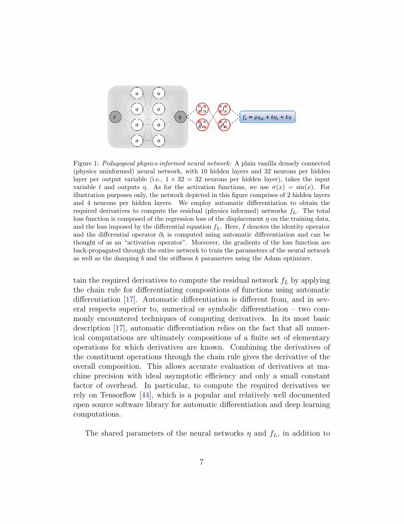
Figure 1: Pedagogical physics-informed neural network: A plain vanilla densely connected(physics uninformed) neural network, with 10 hidden layers and 32 neurons per hiddenlayer per output variable (i.e., 1 × 32 = 32 neurons per hidden layer), takes the inputvariable t and outputs η. As for the activation functions, we use σ(x) = sin(x). Forillustration purposes only, the network depicted in this figure comprises of 2 hidden layersand 4 neurons per hidden layers. We employ automatic differentiation to obtain therequired derivatives to compute the residual (physics informed) networks fL. The totalloss function is composed of the regression loss of the displacement η on the training data,and the loss imposed by the differential equation fL. Here, I denotes the identity operatorand the differential operator ∂t is computed using automatic differentiation and can bethought of as an “activation operator”. Moreover, the gradients of the loss function areback-propagated through the entire network to train the parameters of the neural networkas well as the damping b and the stiffness k parameters using the Adam optimizer.

tain the required derivatives to compute the residual network fL by applyingthe chain rule for differentiating compositions of functions using automaticdifferentiation [17]. Automatic differentiation is different from, and in sev-eral respects superior to, numerical or symbolic differentiation – two com-monly encountered techniques of computing derivatives. In its most basicdescription [17], automatic differentiation relies on the fact that all numer-ical computations are ultimately compositions of a finite set of elementaryoperations for which derivatives are known. Combining the derivatives ofthe constituent operations through the chain rule gives the derivative of theoverall composition. This allows accurate evaluation of derivatives at ma-chine precision with ideal asymptotic efficiency and only a small constantfactor of overhead. In particular, to compute the required derivatives werely on Tensorflow [44], which is a popular and relatively well documentedopen source software library for automatic differentiation and deep learningcomputations.

The shared parameters of the neural networks η and fL, in addition to

7

the damping b and the stiffness k parameters, can be learned by minimizingthe following sum of squared errors loss function

N∑n=1

|η(tn)− ηn|2 +N∑

n=1

|fL(tn)− fnL |2. (3)

The first summation in this loss function corresponds to the training dataon the displacement η(t) while the second summation enforces the dynamicsimposed by equation (1).

2.2. Inferring Lift and Drag Forces from Scattered Velocity Measurements

So far, we have been operating under the assumption that we have accessto direct measurements of the lift force fL. In the following, we are going torelax this assumption by recalling that the fluid motion is governed by theincompressible Navier-Stokes equations given explicitly by

ut + uux + vuy = −px + Re−1(uxx + uyy),vt + uvx + vvy = −py + Re−1(vxx + vyy)− ηtt,ux + vy = 0.

(4)

Here, u(t, x, y) and v(t, x, y) are the streamwise and crossflow componentsof the velocity field, respectively, while p(t, x, y) denotes the pressure, andRe is the Reynolds number based on the cylinder diameter and the freestream velocity. We consider the incompressible Navier-Stokes equations inthe coordinate system attached to the cylinder, so that the cylinder appearsstationary in time. This explains the appearance of the extra term ηtt in thesecond momentum equation (4).

Problem 1 (VIV-I). Given scattered and potentially noisy measurements{tn, xn, yn, un, vn}Nn=1 of the velocity field1 in addition to the data {tn, ηn}Nn=1

on the displacement and knowing the governing equations of the flow (4), weare interested in reconstructing the entire velocity field as well as the pressurefield in space-time. Such measurements are usually collected only in a smallsub-domain, which may not be appropriate for classical CFD computations

1Take for example the case of reconstructing a flow field from scattered measurementsobtained from Particle Image Velocimetry (PIV) or Particle Tracking Velocimetry (PTV).

8

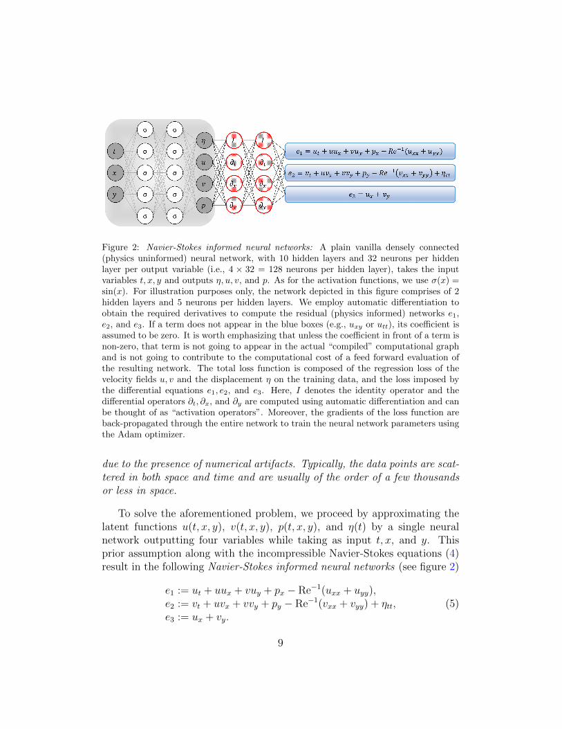
Figure 2: Navier-Stokes informed neural networks: A plain vanilla densely connected(physics uninformed) neural network, with 10 hidden layers and 32 neurons per hiddenlayer per output variable (i.e., 4 × 32 = 128 neurons per hidden layer), takes the inputvariables t, x, y and outputs η, u, v, and p. As for the activation functions, we use σ(x) =sin(x). For illustration purposes only, the network depicted in this figure comprises of 2hidden layers and 5 neurons per hidden layers. We employ automatic differentiation toobtain the required derivatives to compute the residual (physics informed) networks e1,e2, and e3. If a term does not appear in the blue boxes (e.g., uxy or utt), its coefficient isassumed to be zero. It is worth emphasizing that unless the coefficient in front of a term isnon-zero, that term is not going to appear in the actual “compiled” computational graphand is not going to contribute to the computational cost of a feed forward evaluation ofthe resulting network. The total loss function is composed of the regression loss of thevelocity fields u, v and the displacement η on the training data, and the loss imposed bythe differential equations e1, e2, and e3. Here, I denotes the identity operator and thedifferential operators ∂t, ∂x, and ∂y are computed using automatic differentiation and canbe thought of as “activation operators”. Moreover, the gradients of the loss function areback-propagated through the entire network to train the neural network parameters usingthe Adam optimizer.

due to the presence of numerical artifacts. Typically, the data points are scat-tered in both space and time and are usually of the order of a few thousandsor less in space.

To solve the aforementioned problem, we proceed by approximating thelatent functions u(t, x, y), v(t, x, y), p(t, x, y), and η(t) by a single neuralnetwork outputting four variables while taking as input t, x, and y. Thisprior assumption along with the incompressible Navier-Stokes equations (4)result in the following Navier-Stokes informed neural networks (see figure 2)

e1 := ut + uux + vuy + px − Re−1(uxx + uyy),e2 := vt + uvx + vvy + py − Re−1(vxx + vyy) + ηtt,e3 := ux + vy.

(5)

9

We use automatic differentiation [17] to obtain the required derivatives tocompute the residual networks e1, e2, and e3. The shared parameters of theneural networks u, v, p, η, e1, e2, and e3 can be learned by minimizing thesum of squared errors loss function∑N

n=1 (|u(tn, xn, yn)− un|2 + |v(tn, xn, yn)− vn|2)

+∑N

n=1 |η(tn)− ηn|2 +∑3

i=1

∑Nn=1 (|ei(tn, xn, yn)|2) .

(6)

Here, the first two summations correspond to the training data on the fluidvelocity and the structure displacement while the last summation enforcesthe dynamics imposed by equation (4).

The fluid forces on the cylinder are functions of the pressure and thevelocity gradients. Consequently, having trained the neural networks, wecan use

FD =

∮ [−pnx + 2Re−1uxnx + Re−1 (uy + vx)ny

]ds, (7)

FL =

∮ [−pny + 2Re−1vyny + Re−1 (uy + vx)nx

]ds, (8)

to obtain the lift and drag forces exerted by the fluid on the cylinder. Here,(nx, ny) is the outward normal on the cylinder and ds is the arc length onthe surface of the cylinder. We use the trapezoidal rule to approximatelycompute these integrals, and we use equation (8) to obtain the requireddata on the lift force. These data are then used to estimate the structuralparameters b and k by minimizing the loss function (3).

2.3. Inferring Lift and Drag Forces from Flow Visualizations

We now consider the second VIV learning problem by taking one stepfurther and circumvent the need for having access to measurements of thevelocity field by leveraging the following equation

ct + ucx + vcy = Pe−1(cxx + cyy), (9)

governing the evolution of the concentration c(t, x, y) of a passive scalar in-jected into the fluid flow dynamics described by the incompressible Navier-Stokes equations (4). Here, Pe denotes the Peclet number, defined based

10

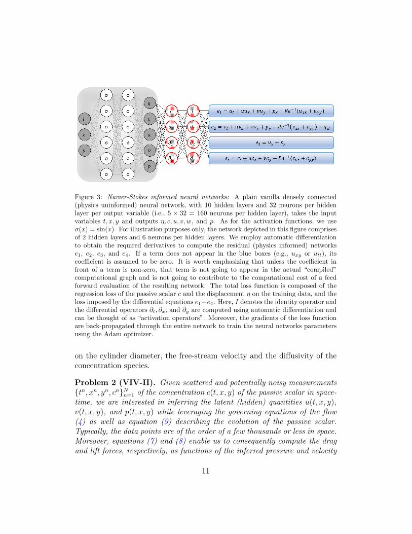
Figure 3: Navier-Stokes informed neural networks: A plain vanilla densely connected(physics uninformed) neural network, with 10 hidden layers and 32 neurons per hiddenlayer per output variable (i.e., 5 × 32 = 160 neurons per hidden layer), takes the inputvariables t, x, y and outputs η, c, u, v, w, and p. As for the activation functions, we useσ(x) = sin(x). For illustration purposes only, the network depicted in this figure comprisesof 2 hidden layers and 6 neurons per hidden layers. We employ automatic differentiationto obtain the required derivatives to compute the residual (physics informed) networkse1, e2, e3, and e4. If a term does not appear in the blue boxes (e.g., uxy or utt), itscoefficient is assumed to be zero. It is worth emphasizing that unless the coefficient infront of a term is non-zero, that term is not going to appear in the actual “compiled”computational graph and is not going to contribute to the computational cost of a feedforward evaluation of the resulting network. The total loss function is composed of theregression loss of the passive scalar c and the displacement η on the training data, and theloss imposed by the differential equations e1−e4. Here, I denotes the identity operator andthe differential operators ∂t, ∂x, and ∂y are computed using automatic differentiation andcan be thought of as “activation operators”. Moreover, the gradients of the loss functionare back-propagated through the entire network to train the neural networks parametersusing the Adam optimizer.

on the cylinder diameter, the free-stream velocity and the diffusivity of theconcentration species.

Problem 2 (VIV-II). Given scattered and potentially noisy measurements{tn, xn, yn, cn}Nn=1 of the concentration c(t, x, y) of the passive scalar in space-time, we are interested in inferring the latent (hidden) quantities u(t, x, y),v(t, x, y), and p(t, x, y) while leveraging the governing equations of the flow(4) as well as equation (9) describing the evolution of the passive scalar.Typically, the data points are of the order of a few thousands or less in space.Moreover, equations (7) and (8) enable us to consequently compute the dragand lift forces, respectively, as functions of the inferred pressure and velocity

11

gradients. Unlike the first VIV problem, here we assume that we do not haveaccess to direct observations of the velocity field.

To solve the second VIV problem, in addition to approximating u(t, x, y),v(t, x, y), p(t, x, y), and η(t) by deep neural networks as before, we representc(t, x, y) by yet another output of the network taking t, x, and y as inputs.This prior assumption along with equation (9) results in the following addi-tional component of the Navier-Stokes informed neural network (see figure3)

e4 := ct + ucx + vcy − Pe−1(cxx + cyy). (10)

The residual networks e1, e2, and e3 are defined as before according toequation (5). We use automatic differentiation [17] to obtain the requiredderivatives to compute the additional residual network e4. The shared pa-rameters of the neural networks c, u, v, p, η, e1, e2, e3, and e4 can be learnedby minimizing the sum of squared errors loss function∑N

n=1 (|c(tn, xn, yn)− cn|2 + |η(tn)− ηn|2)

+∑M

m=1 (|u(tm, xm, ym)− um|2 + |v(tm, xm, ym)− vm|2)

+∑4

i=1

∑Nn=1 (|ei(tn, xn, yn)|2) .

(11)

Here, the first summation corresponds to the training data on the concen-tration of the passive scalar and the structure’s displacement, the secondsummation corresponds to the Dirichlet boundary data on the velocity field,and the last summation enforces the dynamics imposed by equations (4) and(9). Upon training, we use equation (8) to obtain the required data on thelift force. Such data are then used to estimate the structural parameters band k by minimizing the loss function (3).

3. Results2

To generate a high-resolution dataset for the VIV problem we have per-formed direct numerical simulations (DNS) employing the high-order spectral-element method [45], together with the coordinate transformation method

2All data and codes used in this manuscript will be publicly available on GitHub athttps://github.com/maziarraissi/DeepVIV.

12

to take account of the boundary deformation [46]. The computational do-main is [−6.5D, 23.5D] × [−10D, 10D], consisting of 1,872 quadrilateralelements. The cylinder center was placed at (0, 0). On the inflow, locatedat x/D = −6.5, we prescribe (u = U∞, v = 0). On the outflow, wherex/D = 23.5, zero-pressure boundary condition (p = 0) is imposed. On bothtop and bottom boundaries where y/D = ±10, a periodic boundary con-dition is used. The Reynolds number is Re = 100, ρ = 2, b = 0.084 andk = 2.2020. For the case with dye, we assumed the Peclet number Pe = 90.First, the simulation is carried out until t = 1000 D

U∞when the system is

in steady periodic state. Then, an additional simulation for ∆t = 14 DU∞

is performed to collect the data that are saved in 280 field snapshots. Thetime interval between two consecutive snapshots is ∆t = 0.05 D

U∞. Note here

D = 1 is the diameter of the cylinder and U∞ = 1 is the inflow velocity. Weuse the DNS results to compute the lift and drag forces exerted by the fluidon the cylinder. All data and codes used in this manuscript will be publiclyavailable on GitHub at https://github.com/maziarraissi/DeepVIV.

3.1. A Pedagogical Example

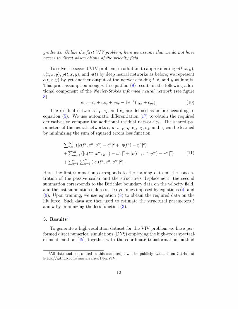
To illustrate the effectiveness of our approach, let us start with the twotime series depicted in figure 4 consisting of N = 111 observations of the dis-placement and the lift force. These data correspond to damping and stiffnessparameters with exact values b = 0.084 and k = 2.2020, respectively. Here,the cylinder is assumed to have a mass of ρ = 2.0. This data-set is then usedto train a 10-layer deep neural network with 32 neurons per hidden layers(see figure 1) by minimizing the sum of squared errors loss function (3) usingthe Adam optimizer [47]. Upon training, the network is used to predict theentire solution functions η(t) and fL(t), as well as the unknown structuralparameters b and k. In addition to almost perfect reconstructions of thetwo time series for displacement and lift force, the proposed framework iscapable of identifying the correct values for the structural parameters b andk with remarkable accuracy. The learned values for the damping and stiff-ness parameters are b = 0.08438281 and k = 2.2015007. This corresponds toaround 0.45% and 0.02% relative errors in the estimated values for b and k,respectively.

As for the activation functions, we use sin(x). In general, the choiceof a neural network’s architecture (e.g., number of layers/neurons and formof activation functions) is crucial and in many cases still remains an art

13

Figure 4: Vortex Induced Vibrations: Observations of the displacement η are plotted inthe left panel while the data on the lift force fL are depicted in the right panel. Theseobservations are shown by the red circles. Predictions of the trained neural networks ηand fL are depicted by blue solid lines.

that relies on one’s ability to balance the trade off between expressivity andtrainability of the neural network [48]. Our empirical findings so far indicatethat deeper and wider networks are usually more expressive (i.e., they cancapture a larger class of functions) but are often more costly to train (i.e.,a feed-forward evaluation of the neural network takes more time and theoptimizer requires more iterations to converge). Moreover, the sinusoid (i.e.,sin(x)) activation function seems to be numerically more stable than tanh(x),at least while computing the residual neural networks fL, and ei, i = 1, . . . , 4(see figures 1, 2, and 3). In this work, we have tried to choose the neuralnetworks’ architectures in a consistent fashion throughout the manuscriptby setting the number of layers to 10 and the number of neurons to 32.Consequently, there might exist other architectures that improve some of theresults reported in the current work.

3.2. Inferring Lift and Drag Forces from Scattered Velocity Measurements

Let us now consider the case where we do not have access to direct mea-surements of the lift force fL. In this case, we can use measurements of thevelocity field, obtained for instance via Particle Image Velocimetry (PIV) orParticle Tracking Velocimetry (PTV), to reconstruct the velocity field, thepressure, and consequently the drag and lift forces. A representative snap-shot of the data on the velocity field is depicted in the top left and top middlepanels of figure 5. The neural network architectures used here consist of 10layers with 32 neurons in each hidden layer. A summary of our results ispresented in figure 5. The proposed framework is capable of accurately (ofthe order of 10−3) reconstructing the velocity field; however, a more intrigu-

14

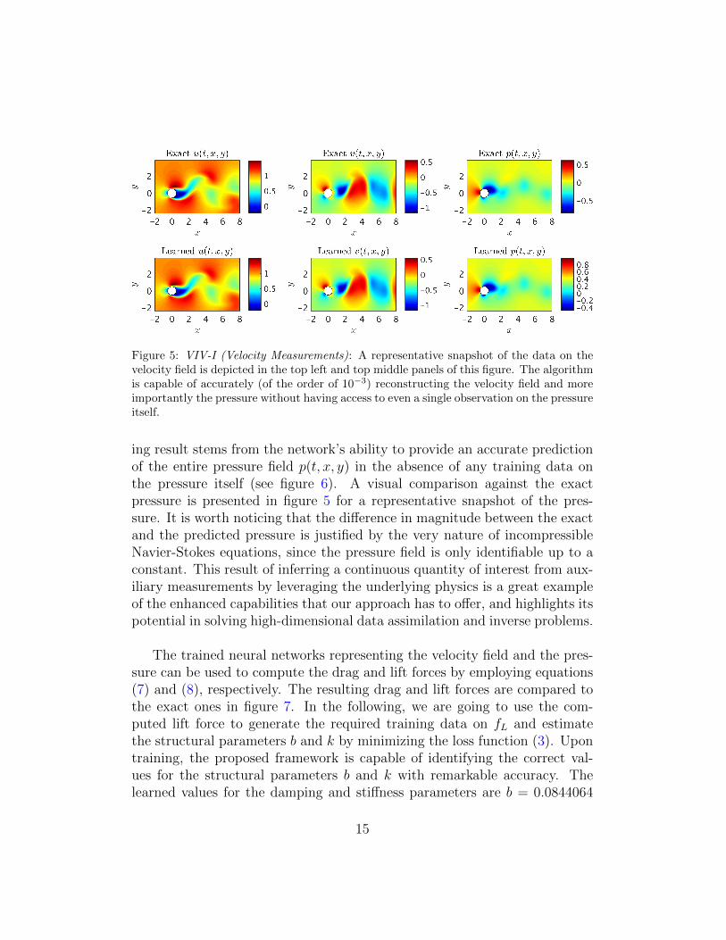
Figure 5: VIV-I (Velocity Measurements): A representative snapshot of the data on thevelocity field is depicted in the top left and top middle panels of this figure. The algorithmis capable of accurately (of the order of 10−3) reconstructing the velocity field and moreimportantly the pressure without having access to even a single observation on the pressureitself.

ing result stems from the network’s ability to provide an accurate predictionof the entire pressure field p(t, x, y) in the absence of any training data onthe pressure itself (see figure 6). A visual comparison against the exactpressure is presented in figure 5 for a representative snapshot of the pres-sure. It is worth noticing that the difference in magnitude between the exactand the predicted pressure is justified by the very nature of incompressibleNavier-Stokes equations, since the pressure field is only identifiable up to aconstant. This result of inferring a continuous quantity of interest from aux-iliary measurements by leveraging the underlying physics is a great exampleof the enhanced capabilities that our approach has to offer, and highlights itspotential in solving high-dimensional data assimilation and inverse problems.

The trained neural networks representing the velocity field and the pres-sure can be used to compute the drag and lift forces by employing equations(7) and (8), respectively. The resulting drag and lift forces are compared tothe exact ones in figure 7. In the following, we are going to use the com-puted lift force to generate the required training data on fL and estimatethe structural parameters b and k by minimizing the loss function (3). Upontraining, the proposed framework is capable of identifying the correct val-ues for the structural parameters b and k with remarkable accuracy. Thelearned values for the damping and stiffness parameters are b = 0.0844064

15

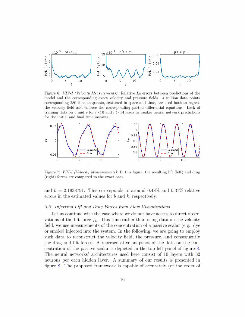
Figure 6: VIV-I (Velocity Measurements): Relative L2 errors between predictions of themodel and the corresponding exact velocity and pressure fields. 4 million data pointscorresponding 280 time snapshots, scattered in space and time, are used both to regressthe velocity field and enforce the corresponding partial differential equations. Lack oftraining data on u and v for t < 0 and t > 14 leads to weaker neural network predictionsfor the initial and final time instants.

Figure 7: VIV-I (Velocity Measurements): In this figure, the resulting lift (left) and drag(right) forces are compared to the exact ones.

and k = 2.1938791. This corresponds to around 0.48% and 0.37% relativeerrors in the estimated values for b and k, respectively.

3.3. Inferring Lift and Drag Forces from Flow Visualizations

Let us continue with the case where we do not have access to direct obser-vations of the lift force fL. This time rather than using data on the velocityfield, we use measurements of the concentration of a passive scalar (e.g., dyeor smoke) injected into the system. In the following, we are going to employsuch data to reconstruct the velocity field, the pressure, and consequentlythe drag and lift forces. A representative snapshot of the data on the con-centration of the passive scalar is depicted in the top left panel of figure 8.The neural networks’ architectures used here consist of 10 layers with 32neurons per each hidden layer. A summary of our results is presented infigure 8. The proposed framework is capable of accurately (of the order of

16

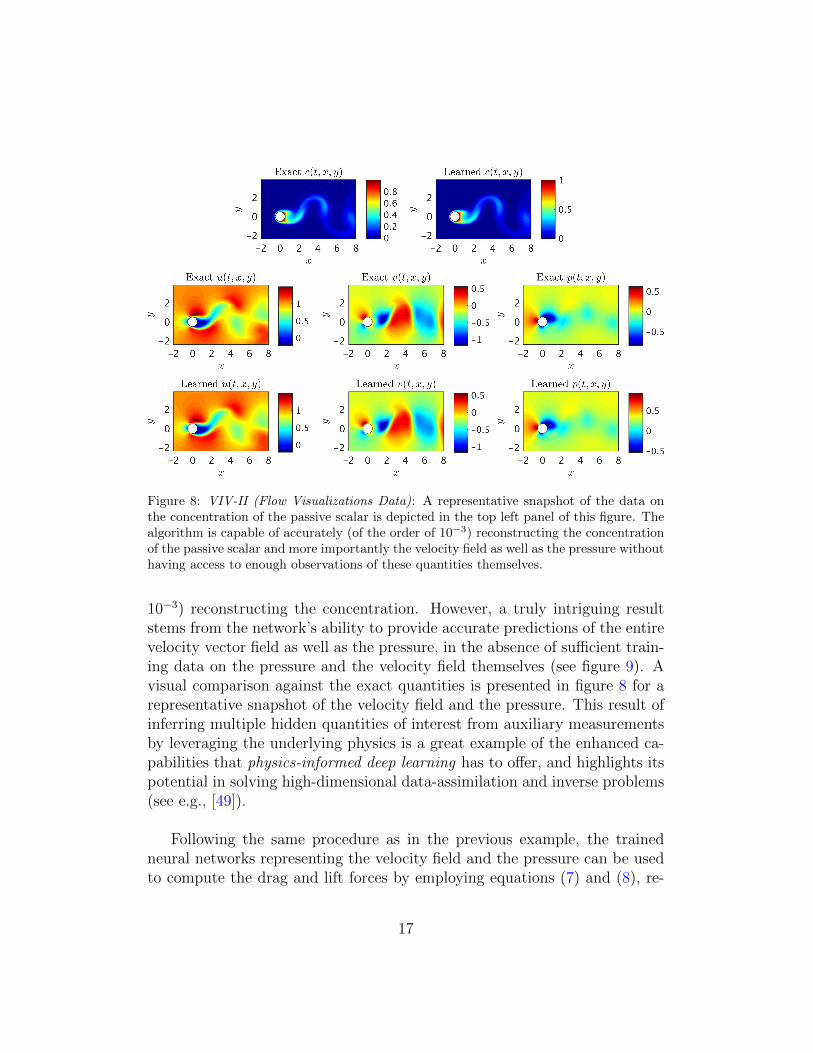
Figure 8: VIV-II (Flow Visualizations Data): A representative snapshot of the data onthe concentration of the passive scalar is depicted in the top left panel of this figure. Thealgorithm is capable of accurately (of the order of 10−3) reconstructing the concentrationof the passive scalar and more importantly the velocity field as well as the pressure withouthaving access to enough observations of these quantities themselves.

10−3) reconstructing the concentration. However, a truly intriguing resultstems from the network’s ability to provide accurate predictions of the entirevelocity vector field as well as the pressure, in the absence of sufficient train-ing data on the pressure and the velocity field themselves (see figure 9). Avisual comparison against the exact quantities is presented in figure 8 for arepresentative snapshot of the velocity field and the pressure. This result ofinferring multiple hidden quantities of interest from auxiliary measurementsby leveraging the underlying physics is a great example of the enhanced ca-pabilities that physics-informed deep learning has to offer, and highlights itspotential in solving high-dimensional data-assimilation and inverse problems(see e.g., [49]).

Following the same procedure as in the previous example, the trainedneural networks representing the velocity field and the pressure can be usedto compute the drag and lift forces by employing equations (7) and (8), re-

17

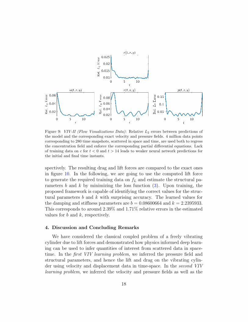
Figure 9: VIV-II (Flow Visualizations Data): Relative L2 errors between predictions ofthe model and the corresponding exact velocity and pressure fields. 4 million data pointscorresponding to 280 time snapshots, scattered in space and time, are used both to regressthe concentration field and enforce the corresponding partial differential equations. Lackof training data on c for t < 0 and t > 14 leads to weaker neural network predictions forthe initial and final time instants.

spectively. The resulting drag and lift forces are compared to the exact onesin figure 10. In the following, we are going to use the computed lift forceto generate the required training data on fL and estimate the structural pa-rameters b and k by minimizing the loss function (3). Upon training, theproposed framework is capable of identifying the correct values for the struc-tural parameters b and k with surprising accuracy. The learned values forthe damping and stiffness parameters are b = 0.08600664 and k = 2.2395933.This corresponds to around 2.39% and 1.71% relative errors in the estimatedvalues for b and k, respectively.

4. Discussion and Concluding Remarks

We have considered the classical coupled problem of a freely vibratingcylinder due to lift forces and demonstrated how physics informed deep learn-ing can be used to infer quantities of interest from scattered data in space-time. In the first VIV learning problem, we inferred the pressure field andstructural parameters, and hence the lift and drag on the vibrating cylin-der using velocity and displacement data in time-space. In the second VIVlearning problem, we inferred the velocity and pressure fields as well as the

18

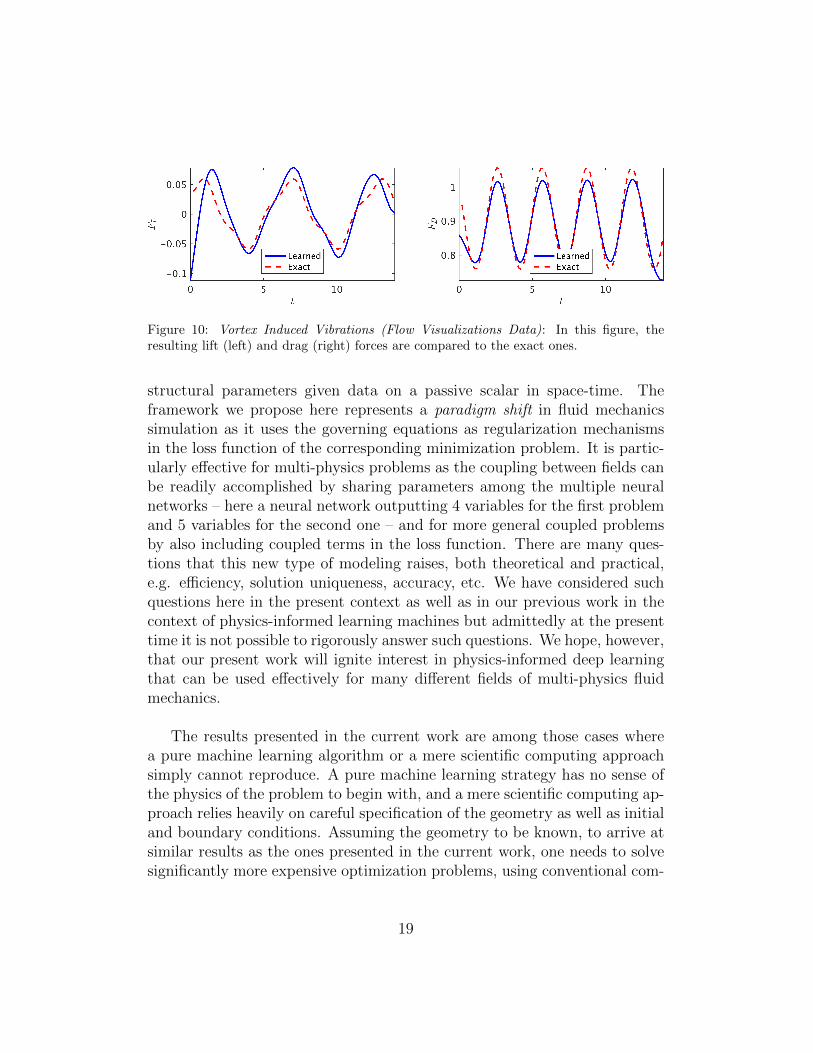
Figure 10: Vortex Induced Vibrations (Flow Visualizations Data): In this figure, theresulting lift (left) and drag (right) forces are compared to the exact ones.

structural parameters given data on a passive scalar in space-time. Theframework we propose here represents a paradigm shift in fluid mechanicssimulation as it uses the governing equations as regularization mechanismsin the loss function of the corresponding minimization problem. It is partic-ularly effective for multi-physics problems as the coupling between fields canbe readily accomplished by sharing parameters among the multiple neuralnetworks – here a neural network outputting 4 variables for the first problemand 5 variables for the second one – and for more general coupled problemsby also including coupled terms in the loss function. There are many ques-tions that this new type of modeling raises, both theoretical and practical,e.g. efficiency, solution uniqueness, accuracy, etc. We have considered suchquestions here in the present context as well as in our previous work in thecontext of physics-informed learning machines but admittedly at the presenttime it is not possible to rigorously answer such questions. We hope, however,that our present work will ignite interest in physics-informed deep learningthat can be used effectively for many different fields of multi-physics fluidmechanics.

The results presented in the current work are among those cases wherea pure machine learning algorithm or a mere scientific computing approachsimply cannot reproduce. A pure machine learning strategy has no sense ofthe physics of the problem to begin with, and a mere scientific computing ap-proach relies heavily on careful specification of the geometry as well as initialand boundary conditions. Assuming the geometry to be known, to arrive atsimilar results as the ones presented in the current work, one needs to solvesignificantly more expensive optimization problems, using conventional com-

19

putational methods (e.g., finite differences, finite elements, finite volumes,spectral methods, and etc.). The corresponding optimization problems in-volve some form of “parametrized” initial and boundary conditions, appro-priate loss functions, and multiple runs of the conventional computationalsolvers. In this setting, one could easily end up with very high-dimensionaloptimization problems that require either backpropagating through the com-putational solvers [50] or “Bayesian” optimization techniques [51] for the sur-rogate models (e.g., Gaussian processes). If the geometry is further assumedto be unknown (as is the case in this work), then its parametrization requiresgrid regeneration, which makes the approach almost impractical.

However, it must be mentioned that we are avoiding the regimes where theNavier-Stokes equations become chaotic and turbulent (e.g., as the Reynoldsnumber increases). In fact, it should not be difficult for a plain vanilla neuralnetwork to approximate the types of complicated functions that naturallyappear in turbulence. However, as we compute the derivatives required inthe computation of the physics informed neural networks (see figures 1, 2,and 3), minimizing the loss functions might become a challenge [7], where theoptimizer may fail to converge to the right values for the parameters of theneural networks. It might be the case that the resulting optimization prob-lem inherits the complicated nature of the turbulent Navier-Stokes equations.Hence, inference of turbulent velocity and pressure fields should be consid-ered in future extensions of this line of research. Moreover, in this work wehave been operating under the assumption of Newtonian and incompressiblefluid flow governed by the Navier-Stokes equations. However, the proposedalgorithm can also be used when the underlying physics is non-Newtonian,compressible, or partially known. This, in fact, is one of the advantages ofour algorithm in which other unknown parameters such as the Reynolds andPeclet numbers can be inferred in addition to the velocity and pressure fields.

Acknowledgements

This work received support by the DARPA EQUiPS grant N66001-15-2-4055 and the AFOSR grant FA9550-17-1-0013. All data and codes used inthis manuscript will be publicly available on GitHub at https://github.

com/maziarraiss/DeepVIV.

20

References

[1] M. P. Paidoussis, Fluid-Structure Interactions: Slender Structures andAxial Flow volume 1, Academic Press, 1998.

[2] M. P. Paidoussis, Fluid-Structure Interactions: Slender Structures andAxial Flow volume 2, Academic Press, 2004.

[3] C. H. K. Williamson, R. Govardhan, Vortex-induced vibration, AnnualReview of Fluid Mechanics 36 (2004) 413–455.

[4] C. Evangelinos, G. E. Karniadakis, Dynamics and flow structures in theturbulent wake of rigid and flexible cylinders subject to vortex-inducedvibrations, Journal of Fluid Mechanics 400 (1999) 91–124.

[5] M. Raissi, P. Perdikaris, G. E. Karniadakis, Physics informed deeplearning (part II): Data-driven discovery of nonlinear partial differentialequations, arXiv preprint arXiv:1711.10566 (2017).

[6] M. Raissi, P. Perdikaris, G. E. Karniadakis, Physics informed deeplearning (part I): Data-driven solutions of nonlinear partial differentialequations, arXiv preprint arXiv:1711.10561 (2017).

[7] M. Raissi, Deep hidden physics models: Deep learning of nonlinearpartial differential equations, arXiv preprint arXiv:1801.06637 (2018).

[8] M. Raissi, P. Perdikaris, G. E. Karniadakis, Inferring solutions of dif-ferential equations using noisy multi-fidelity data, Journal of Computa-tional Physics 335 (2017) 736–746.

[9] M. Raissi, P. Perdikaris, G. E. Karniadakis, Machine learning of lineardifferential equations using Gaussian processes, Journal of Computa-tional Physics 348 (2017) 683 – 693.

[10] H. Owhadi, Bayesian numerical homogenization, Multiscale Modeling& Simulation 13 (2015) 812–828.

[11] C. E. Rasmussen, C. K. Williams, Gaussian processes for machine learn-ing, volume 1, MIT press Cambridge, 2006.

21

[12] M. Raissi, P. Perdikaris, G. E. Karniadakis, Numerical gaussian pro-cesses for time-dependent and nonlinear partial differential equations,SIAM Journal on Scientific Computing 40 (2018) A172–A198.

[13] M. Raissi, G. E. Karniadakis, Hidden physics models: Machine learningof nonlinear partial differential equations, Journal of ComputationalPhysics 357 (2018) 125–141.

[14] H. Owhadi, C. Scovel, T. Sullivan, et al., Brittleness of Bayesian infer-ence under finite information in a continuous world, Electronic Journalof Statistics 9 (2015) 1–79.

[15] G. Pang, L. Yang, G. E. Karniadakis, Neural-net-induced gaussianprocess regression for function approximation and pde solution, arXivpreprint arXiv:1806.11187 (2018).

[16] K. Hornik, M. Stinchcombe, H. White, Multilayer feedforward networksare universal approximators, Neural networks 2 (1989) 359–366.

[17] A. G. Baydin, B. A. Pearlmutter, A. A. Radul, J. M. Siskind, Au-tomatic differentiation in machine learning: a survey, arXiv preprintarXiv:1502.05767 (2015).

[18] R. S. Beidokhti, A. Malek, Solving initial-boundary value problemsfor systems of partial differential equations using neural networks andoptimization techniques, Journal of the Franklin Institute 346 (2009)898–913.

[19] J.-X. Wang, J. Wu, J. Ling, G. Iaccarino, H. Xiao, A comprehensivephysics-informed machine learning framework for predictive turbulencemodeling, arXiv preprint arXiv:1701.07102 (2017).

[20] Y. Zhu, N. Zabaras, Bayesian deep convolutional encoder-decoder net-works for surrogate modeling and uncertainty quantification, arXivpreprint arXiv:1801.06879 (2018).

[21] T. Hagge, P. Stinis, E. Yeung, A. M. Tartakovsky, Solving differen-tial equations with unknown constitutive relations as recurrent neuralnetworks, arXiv preprint arXiv:1710.02242 (2017).

22

[22] R. Tripathy, I. Bilionis, Deep UQ: Learning deep neural network sur-rogate models for high dimensional uncertainty quantification, arXivpreprint arXiv:1802.00850 (2018).

[23] P. R. Vlachas, W. Byeon, Z. Y. Wan, T. P. Sapsis, P. Koumoutsakos,Data-driven forecasting of high-dimensional chaotic systems with long-short term memory networks, arXiv preprint arXiv:1802.07486 (2018).

[24] E. J. Parish, K. Duraisamy, A paradigm for data-driven predictive mod-eling using field inversion and machine learning, Journal of Computa-tional Physics 305 (2016) 758–774.

[25] K. Duraisamy, Z. J. Zhang, A. P. Singh, New approaches in turbulenceand transition modeling using data-driven techniques, in: 53rd AIAAAerospace Sciences Meeting, p. 1284.

[26] J. Ling, A. Kurzawski, J. Templeton, Reynolds averaged turbulencemodelling using deep neural networks with embedded invariance, Jour-nal of Fluid Mechanics 807 (2016) 155–166.

[27] Z. J. Zhang, K. Duraisamy, Machine learning methods for data-driventurbulence modeling, in: 22nd AIAA Computational Fluid DynamicsConference, p. 2460.

[28] M. Milano, P. Koumoutsakos, Neural network modeling for near wallturbulent flow, Journal of Computational Physics 182 (2002) 1–26.

[29] P. Perdikaris, D. Venturi, G. E. Karniadakis, Multifidelity informationfusion algorithms for high-dimensional systems and massive data sets,SIAM J. Sci. Comput. 38 (2016) B521–B538.

[30] R. Rico-Martinez, J. Anderson, I. Kevrekidis, Continuous-time nonlin-ear signal processing: a neural network based approach for gray boxidentification, in: Neural Networks for Signal Processing [1994] IV. Pro-ceedings of the 1994 IEEE Workshop, IEEE, pp. 596–605.

[31] J. Ling, J. Templeton, Evaluation of machine learning algorithms forprediction of regions of high reynolds averaged navier stokes uncertainty,Physics of Fluids 27 (2015) 085103.

23

[32] D. C. Psichogios, L. H. Ungar, A hybrid neural network-first principlesapproach to process modeling, AIChE Journal 38 (1992) 1499–1511.

[33] I. E. Lagaris, A. Likas, D. I. Fotiadis, Artificial neural networks forsolving ordinary and partial differential equations, IEEE Transactionson Neural Networks 9 (1998) 987–1000.

[34] R. Kondor, N-body networks: a covariant hierarchical neural net-work architecture for learning atomic potentials, arXiv preprintarXiv:1803.01588 (2018).

[35] R. Kondor, S. Trivedi, On the generalization of equivariance and con-volution in neural networks to the action of compact groups, arXivpreprint arXiv:1802.03690 (2018).

[36] M. Hirn, S. Mallat, N. Poilvert, Wavelet scattering regression of quan-tum chemical energies, Multiscale Modeling & Simulation 15 (2017)827–863.

[37] S. Mallat, Understanding deep convolutional networks, Phil. Trans. R.Soc. A 374 (2016) 20150203.

[38] R. Bourguet, G. E. Karniadakis, M. S. Triantafyllou, Vortex-inducedvibrations of a long flexible cylinder in shear flow, Journal of FluidMechanics 677 (2011) 342–382.

[39] M. Raissi, Forward-backward stochastic neural networks: Deep learn-ing of high-dimensional partial differential equations, arXiv preprintarXiv:1804.07010 (2018).

[40] M. Raissi, P. Perdikaris, G. E. Karniadakis, Multistep neural networksfor data-driven discovery of nonlinear dynamical systems, arXiv preprintarXiv:1801.01236 (2018).

[41] M. Raissi, Parametric Gaussian process regression for big data, arXivpreprint arXiv:1704.03144 (2017).

[42] P. Perdikaris, M. Raissi, A. Damianou, N. D. Lawrence, G. E. Karni-adakis, Nonlinear information fusion algorithms for data-efficient multi-fidelity modelling, Proc. R. Soc. A 473 (2017) 20160751.

24

[43] M. Raissi, G. Karniadakis, Deep multi-fidelity Gaussian processes, arXivpreprint arXiv:1604.07484 (2016).

[44] M. Abadi, A. Agarwal, P. Barham, E. Brevdo, Z. Chen, C. Citro, G. S.Corrado, A. Davis, J. Dean, M. Devin, et al., Tensorflow: Large-scalemachine learning on heterogeneous distributed systems, arXiv preprintarXiv:1603.04467 (2016).

[45] G. E. Karniadakis, S. Sherwin, Spectral/hp Element Methods for Com-putational Fluid Dynamics, 2nd edition, Oxford University Press, Ox-ford,UK, 2005.

[46] D. J. Newman, G. E. Karniadakis, A direct numerical simulation studyof flow past a freely vibrating cable, Journal of Fluid Mechanics 344(1997) 95–136.

[47] D. P. Kingma, J. Ba, Adam: A method for stochastic optimization,arXiv preprint arXiv:1412.6980 (2014).

[48] M. Raghu, B. Poole, J. Kleinberg, S. Ganguli, J. Sohl-Dickstein,On the expressive power of deep neural networks, arXiv preprintarXiv:1606.05336 (2016).

[49] M. Raissi, A. Yazdani, G. E. Karniadakis, Hidden fluid mechanics:A navier-stokes informed deep learning framework for assimilating flowvisualization data, arXiv preprint arXiv:1808.04327 (2018).

[50] T. Q. Chen, Y. Rubanova, J. Bettencourt, D. Duvenaud, Neural ordi-nary differential equations, arXiv preprint arXiv:1806.07366 (2018).

[51] B. Shahriari, K. Swersky, Z. Wang, R. P. Adams, N. De Freitas, Takingthe human out of the loop: A review of bayesian optimization, Proceed-ings of the IEEE 104 (2016) 148–175.

25