Ch.9 The Consumption Capital Asset Pricing Model

• 9.1 Introduction

• 9.2 The Representative Agent Hypothesis and Its Notion of Equilibrium

• 9.3 An Exchange (Endowment) Economy

• 9.4 Pricing Arrow-Debreu State-Contingent Claims with the CCAPM

• 9.5 Testing the Consumption CAPM: The Equity Premium Puzzle

• 9.6 Testing the Consumption CAPM: Hansen-Jagannathan Bounds

• 9.7 Some Extensions

• 9.8 Conclusions

9.2 The Representative Agent Hypothesis and Its Notion of Equilibrium

• 9.2.1 An Infinitely Lived Representative Agent– Avoid terminal period problem

– Equivalence with finite lives if operative bequest motive

• 9.2.2 On the Concept of a « No-Trade » Equilibrium– Positive net supply: the representative agent willingly hold total

supply

– Zero net supply: at the prevailing price, supply = demand = 0

9.3 An Exchange (Endowment) Economy

- Recursive trading – many periods; investment decisions are made one period at a time, taking due account of their impacton the future state of the world- One perfectly divisible share- Dividend = economy’s total output- Output arises exogenously and stochastically (fruit tree) - Stationary stochastic process

Probability Transition Matrix

Table 9-1 Three-State Probability Transaction Matrix output in period t+1

1Y 2Y 3Y

output in period t

333231

232221

131211

3

2

1

Y

Y

Y =

it

j1tt1t YY,YYobPr)YY(G

- Lucas fruit tree- Grafting an aggregate ouput process- Rational expectations economy: knowledge of the economic structure and the stochastic process

1t1t1t1ttt1 Y~

p~)c~(UEp)c(U (9.1)

ijj

jj1t

j1t1

it

it1 Y

~)Y

~(p))Y

~(c(U)Y(p))Y(c(U

t,1z

zpYzzpc .t.s

)c~(UEmax

t

tttt1ttt

0tt

t

z t

F.O.C:

(i) , i.e., the representative agent owns the entire security;

(ii) , i.e., ownership of the entire security entitles the agent to all the economy's output and,

(iii) , i.e., the agents’ holdings of the security are optimal given the prevailing prices. Substituting (ii) into (iii) informs us that the equilibrium price must satisfy:

1...zzz 2t1tt

tt Yc

)Y~

p~)(c~(UEp)c(U 1t1t1tltttl

1t1t1t1ttt1 Y~

p~)Y~

(UEp)Y(U (9.2)

Definition of an equilibrium

Euler Equation

1t,j1t,j1t1tt1t,j Y~

p~)c~(UE)c(Up

1t

t1

t1tt Y

~)c(U

)c~(UEp

1 f

tt

1ttt )r1(

Y~

EY~

Ep

(9.3)

(9.4)

(9.5)

- Discounting at the IMRS of the representative agent!- Assume risk neutrality:

9.3.2 Interpreting the Exchange Equilibrium

t,j

1t,j1t,j1t,j p

Ypr1

)r~1()c(U

)c~(UE1 1t,j

t1

1t1t

1)c~(UE)c(Uq 1t1tt1bt

)c(U

)c~(UEq

r1

1

t1

1t1t

bt

1t,f

(9.6)

(9.7)

=>Link between discount factor and risk-free rate in a risk neutral world

1t,jt1

1t1t1t,jt

t1

1t1t r~,

)c(U

)c~(Ucovr~1E

)c(U

)c~(UE1

1t,j

t1

1t1t

1t,f

1t,j r~,)c(U

)c~(Ucov

r1

r11

1t,j

t1

1t1t

1t,f

1t,j r~,)c(U

)c~(Ucov1

r1

r1

1t,j

t1

1t1t1t,f1t,f1t,j r~,

)c(U

)c~(Ucovr1rr

, or, rearranging,

, or

(9.8)

(9.9)

Interpreting the CCAPM

• Risk premium is large for those securities paying high returns when consumption is high (MU is low) and low returns when consumption is low.

• Intuition not far from CAPM, but CCAPM adopts consumption smoothing perspective

• The key to an asset’s value is its covariation with the MU of consumption rather than the MU of wealth

t

1t1t,jt1t,f1t,f1t,j bca

c~ba,r~covr1rr

)b(c~,r~covbca

1r1 1t1t,jt

t1t,f

1t1t,jtt

1t,f1t,f1t,j c~,r~cov

bca

r1brr

(9.10)

2ttt c

2

bac)c(U

tt1 bca)c(U

Let

One step further: towards a CAPM equation

Marginal utility is inversely proportional to ct

9.3.3 The Formal Consumption CAPM

1t1t,ctt

1t,f1t,f1t,c c~,r~cov

bca

r1brr

(9.11)

1t,f1t,cc,j1t,f1t,j rrrrt (9.13)

1t1t,ct

1t1t,jt

1t,f1t,c

1t,f1t,j

c~,r~cov

c~,r~cov

rr

rr

)c~var(

c~,r~cov)c~var(

c~,r~cov

rr

rr

1t

1t1t,ct

1t

1t1t,jt

1t,f1t,c

1t,f1t,j

1t,f1t,cc,c

c,j1t,f1t,j rrrr

t

t

(9.12)

, or

, or

c denotes portfolio most correlated with consumption

if c,ct =1

9.4 Pricing Arrow-Debreu State-Contingent Claims with the CCAPM

ss;'ssprob)'s(cUss;'ssq)s(cU t1t1t1t1

ss;'ssprob

)s(cU

)'s(cUss;'ssq t1t

1

1t1t

1.

2. s;'sf

)s(cU

)'s(cUs;'sq

1

1

'sss;'sfs;'sq

Finite states

Continuum of states

ss;'ssprob

)s(cU

)'s(cU)s(q tNt

's 1

1NbNt (9.14)

'st

tt1

tt1

t1

's

1t

t1

t1tt

)'s(Y)s,'s(q

ss;'ssprob)'s(Y)c(U

))'s(c(U

Y)c(U

)c(UEp

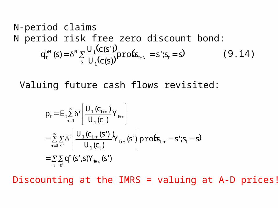
N-period claims N period risk free zero discount bond:

Valuing future cash flows revisited:

Discounting at the IMRS = valuing at A-D prices!

1 t,f

ttt1t

tt1tt

t )r1(

Y~

E)c~(UE)Y

~),c~(Ucov(

1YE

p

1 t,f

tt )r1(

Yp

1 t,f

tt )r1(

]Y~

[Ep

(9.15)

(9.16)

9.5 Testing the Consumption CAPM: The Equity Premium Puzzle

Table 9.1 Properties of U.S. asset returns Annualized data

U.S. Economy

(a) (b) r 6.98 16.54

fr .80 5.67

frr 6.18 16.67 (a) annualized mean values in percent. (b) Annualized standard deviation in percent. Data source : Mehra and Prescott (1985).

1

ccU

1

t

1t

t1

1t1

c

c

)c(U

)c(U

R)x(Rc

c~E1 1t

t

1tt

(9.17)

tt vYp

)c(U

)c~(UY~

Y~

vEvYt1

1t11t1ttt

1t

t

1t x~Y

Y~

1vEv

1

1t

11t

x~E1

x~Ev

t

1t

t

1t1t1t1t Y

Y

v

1v

p

Ypr1R

1t1t1tt x~Ev

1v)R

~(ER

~E

11t

1t

x~E

x~E

bt

1t,f q

1R

1

t1

1t1t )c(U

)c~(UE

1tx~E

11(9.18)

11t

1t1t

f

1t

x~E

x~Ex~E

R

R~

E 2xexp

2xfRlnERln

(9.19)

24.5000123.

008.10698.1ERlnERln2x

f

2(.00123) = .002 = (ln(ER)-ln(ERf) ER – ERf (9.20)

9.6 Testing the Consumption CAPM: Hansen-Jagannathan Bounds

)c(U

))s~(c(U)s~(m

t1

1t1t11t1t

]R~

m~[E1 1t1tt

]R~

m~[E1

]X~

m~[Ep 1t1ttt (9.22)

]s);s~(X)s~(m[E)s(p t1t1t1t1ttt (9.21)

0)]R~

R~

( m~[E ji

0]R~

m~[E ji

, or

0)R~

,m~cov(R~

E m~E jiji

0)R~

,m~(R~

E m~EjiRmjiji

0m~E

)R~

,m~(R~

Em

jiR

ji

ji

m~E)R

~,m~(

R~

Em

jiR

ji

ji

, or

, or

, or

37.167.

062.)rr~(E

m~EfM rr

fMm

)exp(m~E 2x

221

x = . 99 (.967945) = .96 for = 2.

jiR

jimR~

E

m~E

(9.24)