Vector Calculus

CHAPTER 9.1 ~ 9.4

Ch9.1~9.4_2

Contents

9.1 Vector Functions9.2 Motion in a Curve9.3 Curvature and Components of Acceleration9.4 Partial Derivatives

Ch9.1~9.4_3

9.1 Vector Functions

IntroductionA parametric curve in space or space curve is a set of ordered (x, y, z), where x = f(t), y = g(t), z = h(t) (1)

Vector-Valued FunctionsVectors whose components are functions of t,

r(t) = <f(t), g(t)> = f(t)i + g(t)j or r(t) = <f(t), g(t), h(t)> = f(t)i + g(t)j + h(t)kare vector functions. See Fig 9.1

Ch9.1~9.4_4

Fig 9.1

Ch9.1~9.4_5

Example 1: Circular Helix

Graph the curve byr(t) = 2cos ti + 2sin tj + tk, t 0

Solutionx2 + y2

= (2cos t)2 + (2sin t)2 = 22

See Fig 9.2. The curve winds upward in spiral or circular helix.

Ch9.1~9.4_6

Fig 9.2

Ch9.1~9.4_7

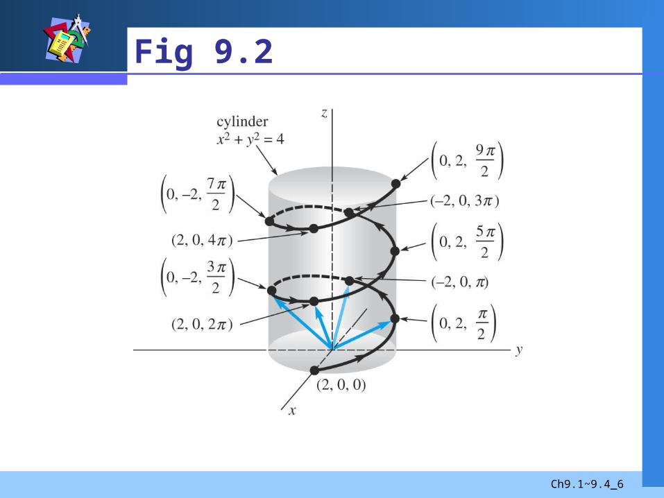
Example 2

Graph the curve byr(t) = 2cos ti + 2sin tj + 3k

Solution x2 + y2

= (2cos t)2 + (2sin t)2 = 22, z = 3See Fig 9.3.

Ch9.1~9.4_8

Fig 9.3

Ch9.1~9.4_9

Example 3

Find the vector functions that describes the curve Cof the intersection of y = 2x and z = 9 – x2 – y2.

SolutionLet x = t, then y = 2t, z = 9 – t2 – 4t2 = 9 – 5t2

Thus, r(t) = ti + 2tj +(9 – 5t2)k. See Fig 9.4.

Ch9.1~9.4_10

Fig 9.4

Ch9.1~9.4_11

If exist, then

DEFINITION 9.1Limit of a Vector Function

)(lim),(lim),(lim thtgtf atatat

)(lim),(lim),(lim)(lim thtgtftatatatat

r

Ch9.1~9.4_12

If , then

(i) , c a scalar

(ii)

(iii)

THEOREM 9.1Properties of Limits

2211 )(lim,)(lim LrLr tt atat

11 )(lim Lr ctcat

2121 )]()([lim LLrr

ttat

2121 )()(lim LLrr ．．

ttat

Ch9.1~9.4_13

A vector function r is said to be continuous at t = a if

(i) r(a) is defined, (ii) limta r(t) exists, and

(iii) limta r(t) = r(a).

DEFINITION 9.2Continuity

The derivative of a vector function r is (2)

for all t which the limits exists.

DEFINITION 9.3Derivative of Vector Function

)]()([1

lim)('0

tttt

tt

rrr

Ch9.1~9.4_14

Proof

If , where f, g, and h are

Differentiable, then

THEOREM 9.2Differentiation of a Components

)(),(),()( thtgtftr

)('),('),(')(' thtgtftr

tthtth

ttgttg

ttfttf

thtgtftthttgttft

t

t

t

)()(,

)()(,

)()(lim

])(),(),()(),(),([1

lim)(

0

0r

Ch9.1~9.4_15

Smooth Curve

When the component functions of r have continuous first derivatives and r’(t) 0 for t in the interval (a, b), then r is said to be a smooth function, and the corresponding curve is called a smooth curve.

Ch9.1~9.4_16

Geometric Interpretation of r’(t)

See Fig 9.5.

)()( ttt rrr

)]()([1

ttttt

rrr

Ch9.1~9.4_17

Fig 9.5

Ch9.1~9.4_18

Example 4

Graph the curve by r(t) = cos 2t i + sin t j, 0 t 2. Graph r’(0) and r’(/6).

Solutionx = cos 2t, y = sin t, then x = 1 – 2y2, −1 x 1

And r’(t) = −2sin 2ti + cos tj,

r’(0) = j, r’(/6) = jir23

36

Ch9.1~9.4_19

Fig 9.6

Ch9.1~9.4_20

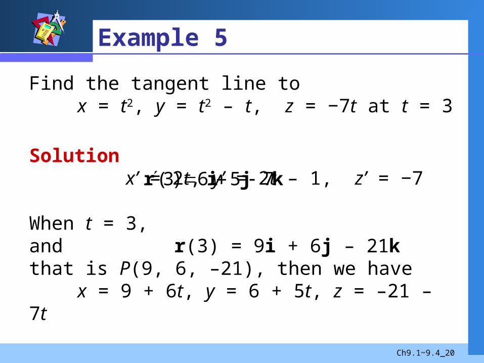
Example 5

Find the tangent line to x = t2, y = t2 – t, z = −7t at t = 3

Solutionx’ = 2t, y’ = 2t – 1, z’ = −7

When t = 3,and r(3) = 9i + 6j – 21kthat is P(9, 6, –21), then we have

x = 9 + 6t, y = 6 + 5t, z = –21 – 7t

kjir 756)3(

Ch9.1~9.4_21

Example 6

If r(t) = (t3 – 2t2)i + 4tj + e-tk, then

r’(t) = (3t2 – 4t)i + 4j − e-tk, and

r”(t) = (6t – 4)i + e-tk.

Ch9.1~9.4_22

If r is a differentiable vector function and s = u(t) is a

differentiable scalar function, then the derivatives of r(s) with respect to t is

THEOREM 9.3Chain Rule

)(')(' tustd

dsdsd

tdd

rrr

Ch9.1~9.4_23

Example 7

If r(s) = cos2si + sin2sj + e–3sk, s = t4, then

kji

kjir

4334343

33

12)2cos(8)2sin(8

4]32cos22sin2[

t

s

ettttt

tessdtd

Ch9.1~9.4_24

If r1 and r2 be differentiable vector functions and u(t)

A differentiable scalar function.

(i)

(ii)

(iii)

(iv)

THEOREM 9.4Chain Rule

)()()]()([ 2121 tttttd

drrrr

)()()()()]()([ 111 ttuttuttutd

drrr

)()()()()]()([ 212121 tttttttd

drrrrrr ．．．

)()()()()]()([ 212121 tttttttd

drrrrrr

Ch9.1~9.4_25

Integrals of Vector Functions

kjir

kjir

b

a

b

a

b

a

b

adtthdttgdttfdtt

dtthdttgdttfdtt

)()()()(

)()()()(

kjir )()()()( thtgtft

Ch9.1~9.4_26

Example 8

If r(t) = 6t2i + 4e–2t j + 8cos 4t k, then

where c = c1i + c2j + c3k.

ckji

kji

kjir

tet

ctcect

dttdtedttdtt

t

t

t

4sin222

]4sin2[]2[]2[

4cos846)(

23

322

13

22

Ch9.1~9.4_27

Length of a Space Curve

If r(t) = f(t)i + g(t)j + h(t)k, then the length of this smooth curve is

(3)

b

a

b

adttdtthtgtfs ||)(||)]([)]([)]([ 222 r

Ch9.1~9.4_28

Example 9

Consider the curve in Example 1. Since , from (3) the length from r(0) to r(t) is

Using then (4)

Thus

5||)('|| tr

tdust

550

5/st

kjir55

sin25

cos2)(sss

s

5)(,

5sin2)(,

5cos2)(

ssh

ssg

ssf

Ch9.1~9.4_29

9.2 Motion on a Curve

Velocity and AccelerationConsider the position vector

r(t) = f(t)i + g(t)j + h(t)k, then

kjira

kjirv

)()()()()(

)()()()()(

thtgtftt

thtgtftt

222

||)(||

dt

dz

dt

dy

dt

dx

dt

dt

rv

||)(||)( tts v1

0

||)(||t

tts v

Ch9.1~9.4_30

Example 1

Position vector: r(t) = t2i + tj + (5t/2)k. Graph the curve defined by r(t) and v(2), a(2).

Solution

so that See Fig 9.7.

,25

2)()( kjirv ttt ira 2)()( tt

iakjiv 2)2(,2/54)2(

Ch9.1~9.4_31

Fig 9.7

Ch9.1~9.4_32

Note:

‖v(t)‖2 = c2 or v‧v = c2

a(t)‧v(t) = 0

02)( dt

d

dt

d

dt

d

dt

d vvv

vvvvv ．．．．

0vv．

dt

d

Ch9.1~9.4_33

Example 2

Consider the position vector in Example 2 of Sec 9.1. Graph the velocity and acceleration at t = /4.

SolutionRecall r(t) = 2cos ti + 2sin tj + 3k.then v(t) = −2sin ti + 2cos tj

a(t) = −2cos ti −2sin t jand

jijia

jijiv

224

sin24

cos24

224

cos24

sin24

Ch9.1~9.4_34

Fig 9.8

Ch9.1~9.4_35

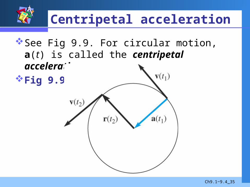
Centripetal acceleration

See Fig 9.9. For circular motion, a(t) is called the centripetal acceleration.

Fig 9.9

Ch9.1~9.4_36

Curvilinear Motion in the Plane

See Fig 9.10. Acceleration of gravity : −gjAn initial velocity: v0 = v0 cos i + v0 sin j from an initial height s0 = s0 j, then

where v(0) = v0, then c1 = v0. Therefore

v(t) = (v0cos )i + (– gt + v0sin )j

1)()( cgtdtgt jjv

Ch9.1~9.4_37

Integrating again and using r(0) = s0,

Hence we have

(1)

See Fig 9.11

jir

00

20 )sin(

2

1)cos()( stvgttvt

002

0 )sin(2

1)(,)cos()( stvgttytvtx

Ch9.1~9.4_38

Fig 9.10

Ch9.1~9.4_39

Fig 9.11

Ch9.1~9.4_40

Example 3

A shell is fired from ground level with v0 = 768 ft/s at an angle of elevation 30 degree. Find (a) the vector function and the parametric equations of the trajectory, (b) the maximum attitude attained, (c) the range of the shell (d) the speed of impact.

Solution(a) Initially we have s0 = 0, and

(2)

jijiv 3843384)30sin768()30cos768(0

Ch9.1~9.4_41

Example 3 (2)

Since a(t) = −32j and using (2) gives (3)

Integrating again,

Hence the trajectory is(4)

(b) From (4), we see that dy/dt = 0 when −32t + 384 = 0 or t = 12. Thus the maximum height H is

H = y(12) = – 16(12)2 + 384(12) = 2304 ft

jiv )38432()3384()( tt

jir )38416()3384()( 2 tttt

tttyttx 38416)(,3384)( 2

Ch9.1~9.4_42

Example 3 (3)

(c) From (4) we see that y(t) = 0 when −16t(t – 24) = 0, or t = 0, 24.

Then the range R is

(d) from (3), we obtain the impact speed of the shell

ft963,15)24(3384)24( xR

ft/s768)3384()384(||)24(|| 22 v

Ch9.1~9.4_43

9.3 Curvature and Components of Acceleration

Unit TangentWe know r’(t) is a tangent vector to the curve C, then

(1)

is a unit tangent. Since the curve is smooth, we also have ds/dt = ||r’(t)|| > 0. Hence

(2)

See Fig 9.19.

||)(||)(

tt

rr

T

,dtds

dsd

dtd rr T

rrrr

||)(||

)(//

tt

dtdsdtd

dsd

Ch9.1~9.4_44

Fig 9.16

Ch9.1~9.4_45

Rewrite (3) as

that is, (4)

From (2) we have T = dr/ds, then the curvature of C

at a point is(3)

DEFINITION 9.4Curvature

dsdT

,dtds

dsd

dtd TT

dtdsdtd

dsd

//TT

||r||T

)(||)(||

tt

Ch9.1~9.4_46

Example 1

Find the curvature of a circle of radius a.

SolutionWe already know the equation of a circle isr(t) = a cos ti + a sin tj, then

We get

Thus, (5)

and cossin||)(||

)()( ji

rr

T tttt

t

jiT ttt sincos)(

aatt

tt 1sincos

||)(||||)(|| 22

rT

and cossin)( jir tatat at ||)(|| r

Ch9.1~9.4_47

Fig 9.17

Ch9.1~9.4_48

Tangential and Normal Components

Since T is a unit tangent, then v(t) = ||v(t)||T = vT, then

(6)Since T T = 1 so that T dT/dt = 0 (Theorem 9.4),we have T and dT/dt are orthogonal. If ||dT/dt|| 0, then

(7)is a unit normal vector to C at a point P with the direction given by dT/dt. See Fig 9.18.

||/||/dtddtd

TT

N

TT

adtdv

dtd

vt )(

Ch9.1~9.4_49

Fig 9.18

Ch9.1~9.4_50

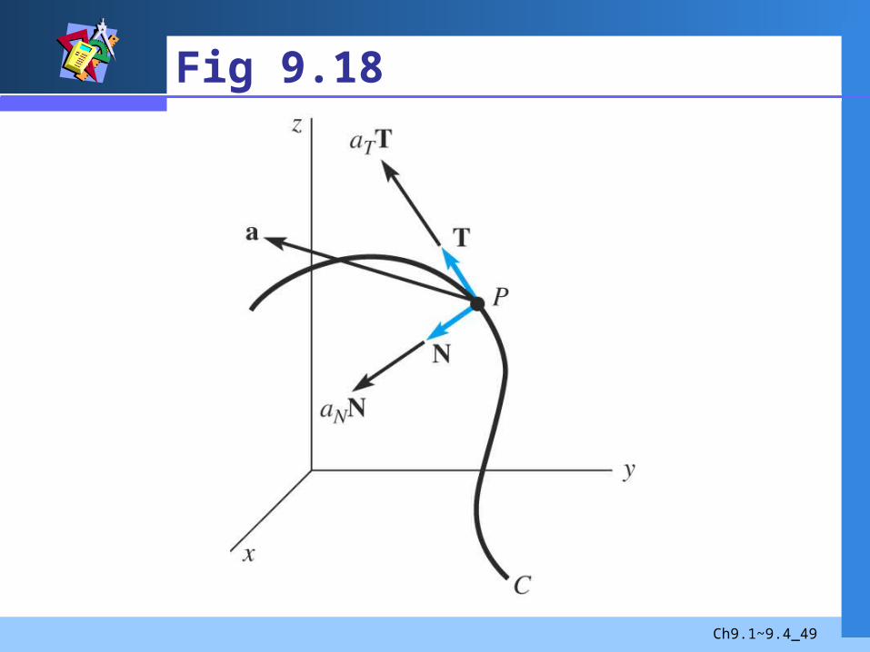
The vector N is also called the principal normal. However =║dT / dt║/ v, from (7) we havedT/dt = vN. Thus (6) becomes

(8)

By writing (8) as a(t) = aNN + aTT (9)

Thus the scalar functions aN and aT are called the tangential and normal components.

TNadt

dvvt 2)(

Ch9.1~9.4_51

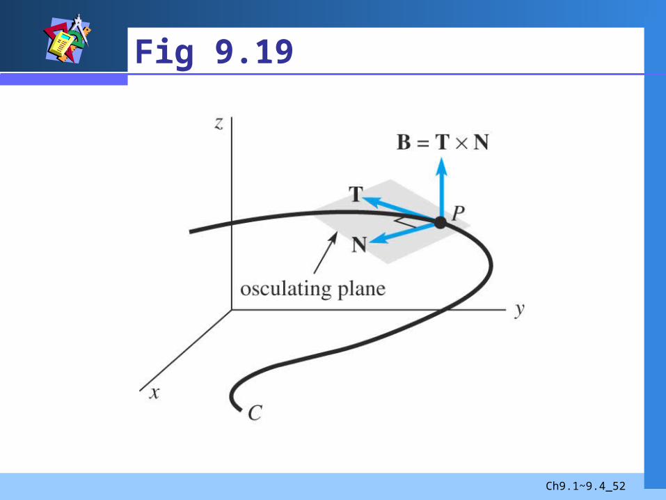
The Binormal

A third vector defined byB = T N

is called the binormal. These three vectors T, N, Bform a right-hand set of mutually orthogonal vectors called the moving trihedral. The plane of T and T is called the osculating plane, the plane of N and B is called the rectifying plane. See Fig 9.19.

Ch9.1~9.4_52

Fig 9.19

Ch9.1~9.4_53

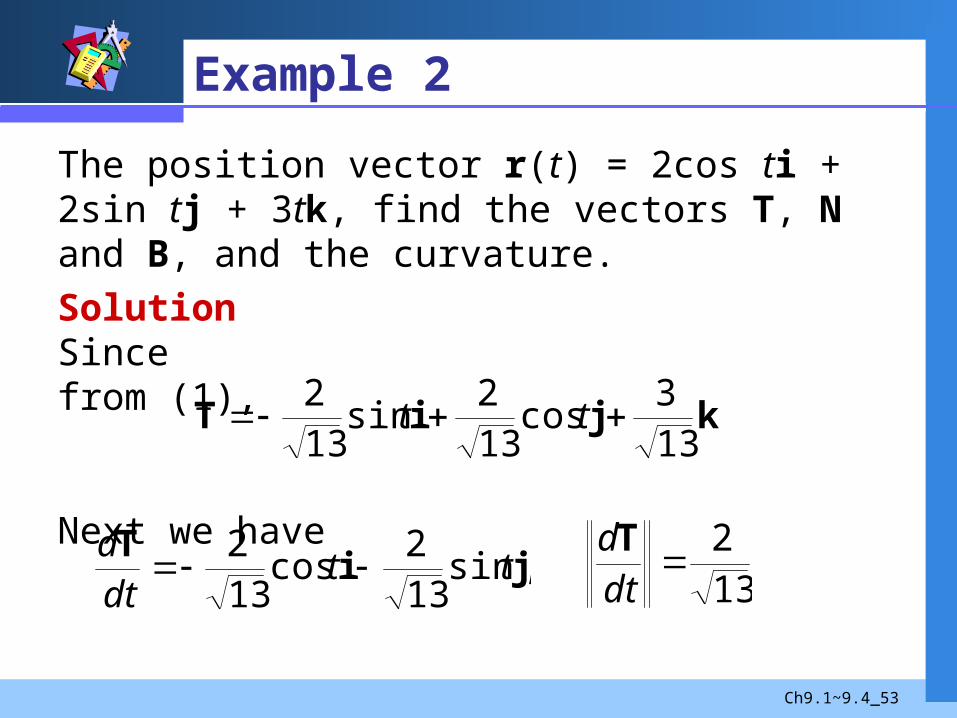
Example 2

The position vector r(t) = 2cos ti + 2sin tj + 3tk, find the vectors T, N and B, and the curvature.

SolutionSincefrom (1),

Next we have

kjiT133

cos132

sin132 tt

,sin132

cos132

jiT

ttdtd

132

dtdT

Ch9.1~9.4_54

Example 2 (2)

Hence (3) gives N = – cos ti – sin tj

Now,

Finally using and

kji

kji

NTB

132

cos133

sin133

0sincos133

cos132

sin132

tt

tt

tt

13/2||/|| tddT 13||)(|| tr

Ch9.1~9.4_55

Example 2 (3)

From (4) we have

132

1313/2

Ch9.1~9.4_56

Formula for aT, aN and Curvature

Observe

then

(10)

On the other hand

vavava TTN )()(10

TTNTav ．．．

||r||rr

vav

)()()(

|||| ttt

dtdv

aT

．．

BTTNTav0B

vavava NTN )()(

Ch9.1~9.4_57

Since ||B|| = 1, it follows that

(11)

then(12)

||r||rr

vav

)(||)()(||

||||||||2

ttt

vaN

3||r||

rr

v

av

)(

||)()(||

||||

||||3 t

tt

Ch9.1~9.4_58

Example 3

The position vector r(t) = ti + ½t2j + (1/3)t3k is said to be a “twisted” cube”. Find the tangential and normal components of the acceleration at t. Find the curvature.

Solution

Since v a = t + 2t3 and From (10),

kjrakjirv ttttttt 2)()(,)()( 2

42

3

1

2

tt

ttdtdv

aT

Ch9.1~9.4_59

Example 3 (2)

Now

and

From (11)

From (12)

kji

kji

av tt

t

tt 2

210

1 22

14|||| 24 ttav

1

14

1

1424

24

42

242

tt

tt

tt

ttvaN

2/324

2/124

)1(

)14(

tt

tt

Ch9.1~9.4_60

Radius of Curvatures

= 1/ is called the radius of curvature. See Fig 9.20.

Ch9.1~9.4_61

9.4 Partial Derivatives

Functions of Two VariablesSee Fig 9.21. The graph of a function z = f(x, y) is a surface in 3-space.

Ch9.1~9.4_62

Fig 9.21

Ch9.1~9.4_63

Level Curves

The curves defined by f(x, y) = c are called the level curves of f. See Fig 9.22.

Ch9.1~9.4_64

Example 1

The level curves of f(x, y) = y2 – x2 are defined by y2 – x2 = c. See Fig 9.23. For c = 0, we obtain the lines y = x, y = −x.

Ch9.1~9.4_65

Level Surfaces

The level surfaces of w = F(x, y, z) are defined by F(x, y, z) = c.

Ch9.1~9.4_66

Example 2

Describe the level curves of F(x, y, z) = (x2 + y2)/z.

SolutionFor c 0, (x2 + y2)/z = c, or x2 + y2 = cz. See Fig 9.24. ，

Ch9.1~9.4_67

Fig 9.24

Ch9.1~9.4_68

Partial Derivatives

For y = f(x),

For z = f(x, y),

(1)

(2)

xyxfyxxf

xz

x

),(),(lim

0

xxfxxf

dxdy

x

)()(lim

0

yyxfyyxf

yz

y

),(),(lim

0

Ch9.1~9.4_69

Example 3

If z = 4x3y2 – 4x2 + y6 + 1, find ,

Solutionxz

yz

xyxxz

812 22

53 68 yyxyz

Ch9.1~9.4_70

Alternative Symbols

If z = f(x, y), we have

xx fzxf

xz

yy fzyf

yz

Ch9.1~9.4_71

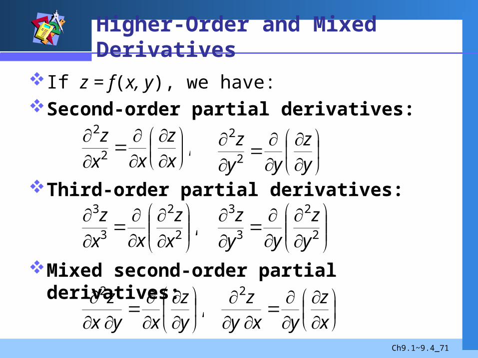
Higher-Order and Mixed Derivatives

If z = f(x, y), we have:Second-order partial derivatives:

Third-order partial derivatives:

Mixed second-order partial derivatives:

,2

2

xz

xx

z

yz

yy

z2

2

,2

2

3

3

x

zxx

z

2

2

3

3

y

zyy

z

,2

yz

xyxz

xz

yxyz2

Ch9.1~9.4_72

Alternative Symbols

If f has continuous second partial derivatives, then

fxy = fyx　　　　　　　　　　(3)

,)(2

xyz

xz

yff yxxy

yxz

f yx

2

Ch9.1~9.4_73

Example 4

If

then

yxetyxF t 6sin4cos),,( 3

yxetyxF

yxetyxF

yxetyxF

tt

ty

tx

6sin4cos3),,(

6cos4cos6),,(

6sin4sin4),,(

3

3

3

Ch9.1~9.4_74

If z = f(u, v) is differentiable, and u = g(x, y) and

v = h(x, y) have continuous first partial derivatives,

then

(5)

THEOREM 9.5Chain Rule

yv

vz

yu

uz

yz

xv

vz

xu

uz

xz

,

Ch9.1~9.4_75

Example 5

If z = u2 – v3, u = e2x – 3y, v = sin(x2 – y2), find andSolutionSincethen

(6)

(7)

xz /yz /

,2/ uuz 23/ vvz

)cos(64

)]cos(2[3)2(2

22232

22232

yxxvue

yxxveuxz

yx

yx

)cos(66

)]cos()2[(3)3(2

22232

22232

yxyvue

yxyveuyz

yx

yx

Ch9.1~9.4_76

Special Case

If z = f(u, v) is differentiable, and u = g(t) and v = h(t) are differentiable, then

(8)

If z = f(u1, u2,…, un) and each variable u1, u2,…, un are functions of x1, x2,…, xk, we have

(9)

dtdv

vz

dtdu

uz

dtdz

i

n

niii xu

uz

xu

uz

xu

uz

xz

2

2

1

1

Ch9.1~9.4_77

Similarly, if u1, u2,…, un are functions of a single variable t, then

(10)

These results can be memorized in terms of a tree diagram. See next page.

dtdu

uz

dtdu

uz

dtdu

uz

dtdz n

n

2

2

1

1

Ch9.1~9.4_78

Ch9.1~9.4_79

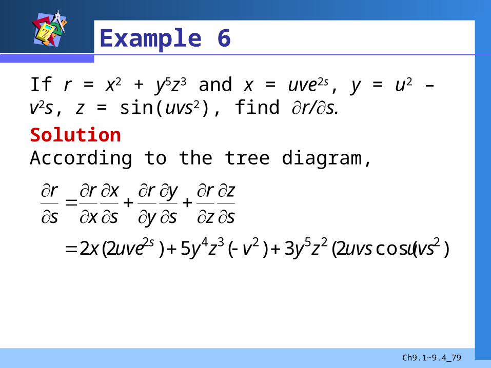
Example 6

If r = x2 + y5z3 and x = uve2s, y = u2 – v2s, z = sin(uvs2), find r/s.

SolutionAccording to the tree diagram,

))cos(2(3)(5)2(2 2252342 uvsuvszyvzyuvex

sz

zr

sy

yr

sx

xr

sr

s

Ch9.1~9.4_80

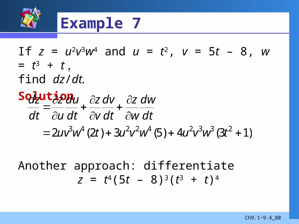
Example 7

If z = u2v3w4 and u = t2, v = 5t – 8, w = t3 + t，find dz/dt.

Solution

Another approach: differentiate z = t4(5t – 8)3(t3 + t)4

)13(4)5(3)2(2 233242243

twvuwvutwuv

dtdw

wz

dtdv

vz

dtdu

uz

dtdz

Ch9.1~9.4_81 Zill工程數學(上)茆政吉譯Zill工程數學(上)茆政吉譯