1

BİL 542

Parallel Computing

2

Parallel Programming

Chapter 1

3

Why Use Parallel Computing?

Main Reasons:

Save time and/or money: In theory, throwing more resources at a task will shorten its time to completion, with potential cost savings. Parallel clusters can be built from cheap, commodity components.

Solve larger problems: Many problems are so large and/or complex that it is impractical or impossible to solve them on a single computer, especially given limited computer memory. For example: Web search engines/databases processing millions of

transactions per second

4

Demand for Computational Speed

Continual demand for greater computational

speed from a computer system than is

currently possible

Areas requiring great computational speed

include numerical modeling and simulation of

scientific and engineering problems.

Computations must be completed within a

“reasonable” time period.

5

Grand Challenge Problems One that cannot be solved in a reasonable amount of time with today’s

computers. Obviously, an execution time of 10 years is always unreasonable.

Examples Databases, data mining

Oil exploration

Web search engines, web based business services

Medical imaging and diagnosis

Pharmaceutical design

Management of national and multi-national corporations

Financial and economic modeling

Advanced graphics and virtual reality, particularly in the entertainment industry

Networked video and multi-media technologies

Collaborative work environments

Modeling large DNA structures

Global weather forecasting

Modeling motion of astronomical bodies.

6

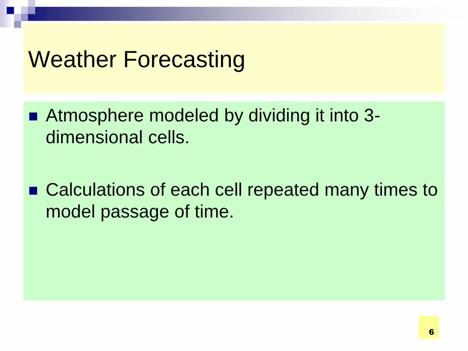
Weather Forecasting

Atmosphere modeled by dividing it into 3-

dimensional cells.

Calculations of each cell repeated many times to

model passage of time.

7

Global Weather Forecasting Example

Suppose whole global atmosphere divided into cells of size 1 mile 1 mile 1 mile to a height of 10 miles (10 cells high) - about 5 108 cells.

Suppose each calculation requires 200 floating point operations. In one time step, 1011 floating point operations necessary.

To forecast the weather over 7 days using 1-minute intervals, a computer operating at 1Gflops (109 floating point operations/s) takes 106 seconds or over 10 days.

To perform calculation in 5 minutes requires computer operating at 3.4 Tflops (3.4 1012 floating point operations/sec).

8

Modeling Motion of Astronomical Bodies

Each body attracted to each other body by

gravitational forces. Movement of each body predicted

by calculating total force on each body.

With N bodies, N - 1 forces to calculate for each body,

or approx. N2 calculations. (N log2 N for an efficient

approx. algorithm.)

After determining new positions of bodies, calculations

repeated.

9

A galaxy might have, say, 1011 stars.

Even if each calculation done in 1 ms (extremely

optimistic figure), it takes 109 years for one

iteration using N2 algorithm and almost a year

for one iteration using an efficient N log2 N

approximate algorithm.

Modeling Motion of Astronomical Bodies

10

Astrophysical N-body simulation by Scott Linssen (undergraduate

UNC-Charlotte student).

11

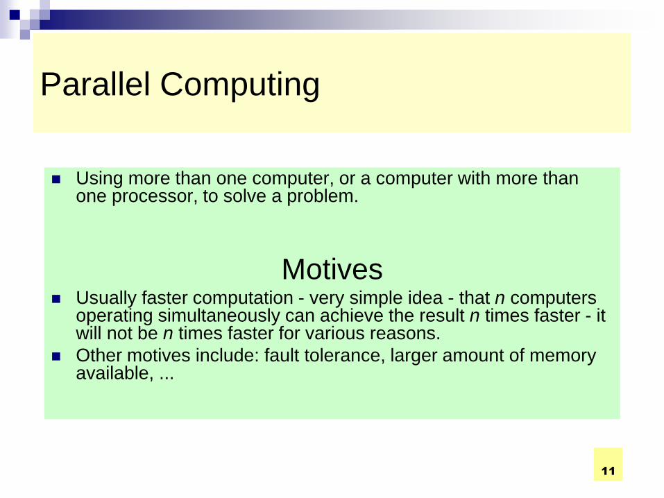
Parallel Computing

Using more than one computer, or a computer with more than one processor, to solve a problem.

Motives Usually faster computation - very simple idea - that n computers

operating simultaneously can achieve the result n times faster - it will not be n times faster for various reasons.

Other motives include: fault tolerance, larger amount of memory available, ...

12

Parallel Computing vs Traditional

Computing

13

Background

Parallel computers - computers with more than

one processor - and their programming - parallel

programming - has been around for more than

40 years.

14

15

Speedup Factor

where ts is execution time on a single processor and tp is execution time on a multiprocessor.

S(p) gives increase in speed by using multiprocessor.

Use best sequential algorithm with single processor system. Underlying algorithm for parallel implementation might be (and is usually) different.

S(p) = Execution time using one processor (best sequential algorithm)

Execution time using a multiprocessor with p processors

ts

tp =

16

Speedup factor can also be cast in terms

of computational steps:

Can also extend time complexity to

parallel computations.

S(p) = Number of computational steps using one processor

Number of parallel computational steps with p processors

17

Maximum Speedup

Maximum speedup is usually p with p processors

(linear speedup).

Possible to get superlinear speedup (greater than

p) but usually a specific reason such as:

Extra memory in multiprocessor system

COMPE472 Parallel Computing 18

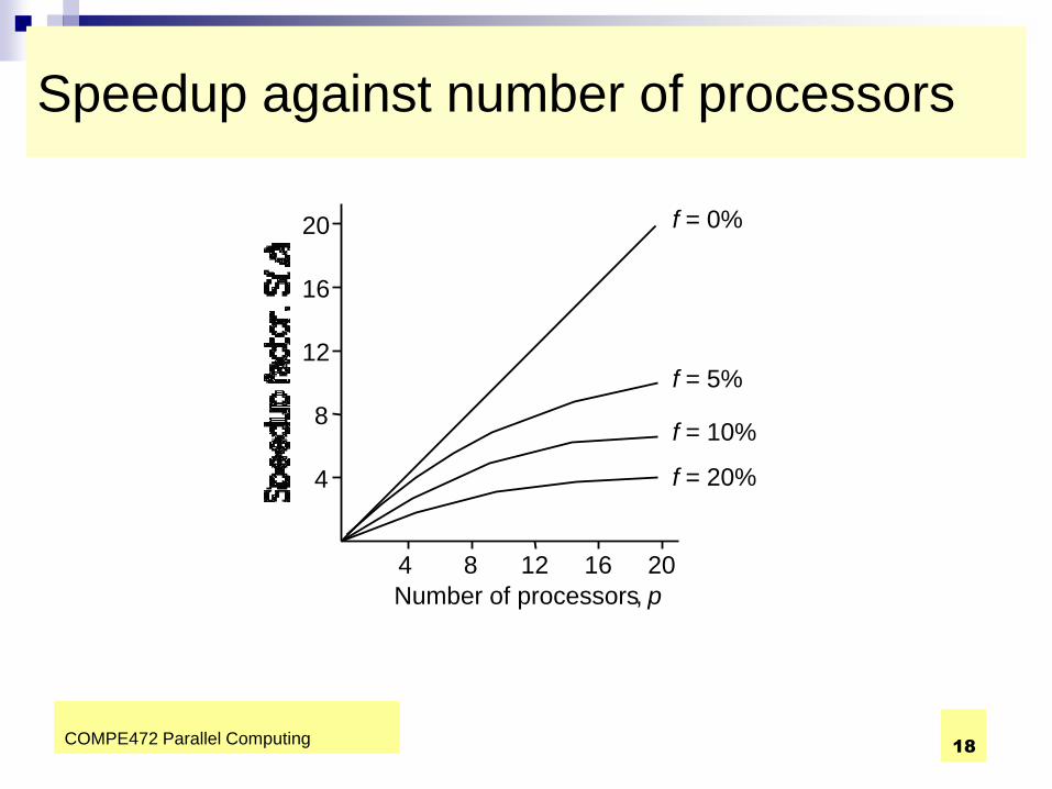
Speedup against number of processors

4

8

12

16

20

4 8 12 16 20

f = 20%

f = 10%

f = 5%

f = 0%

Number of processors , p

COMPE472 Parallel Computing 19

Maximum Speedup

Factors limiting speedup

Communication time

Extra computations in the parallel algorithm

(reevaluation of constants locally)

Idle time of some processors

20

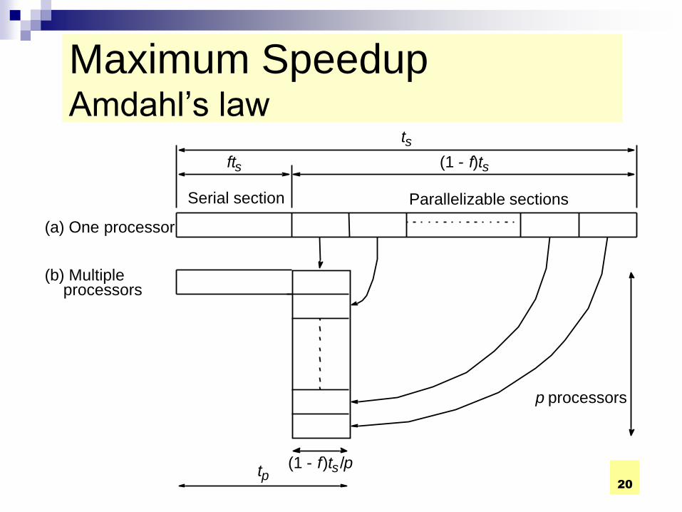
Maximum Speedup Amdahl’s law

Serial section Parallelizable sections

(a) One processor

(b) Multiple processors

ft s (1 - f ) t s

t s

(1 - f ) t s / p t p

p processors

COMPE472 Parallel Computing 21

Speedup factor is given by:

This equation is known as Amdahl’s law

S(p) ts p

fts (1 f )ts /p 1 (p 1)f

Amdahl’s Law

22

Amdahl’s law

Even with infinite number of processors, maximum

speedup is limited :

Example

With only 5% of computation being serial,

maximum speedup is 20, irrespective of number of

processors.

23

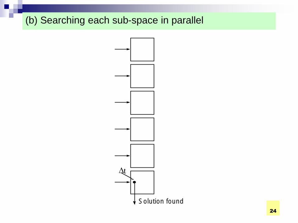
Superlinear Speedup example - Searching

(a) Searching each sub-space sequentially

t s

t s /p

Start Time

D t

Solution found x t s /p

Sub-space search

x indeterminate

24

(b) Searching each sub-space in parallel

Solution found

D t

COMPE472 Parallel Computing 25

Speed-up then given by

S(p)

x t s p

t D +

t D =

26

Worst case for sequential search when solution

found in last sub-space search. Then parallel

version offers greatest benefit.

27

Least advantage for parallel version when

solution found in first sub-space search of

the sequential search, i.e.

Actual speed-up depends upon which

subspace holds solution but could be

extremely large.

S(p) = t D

t D = 1

28

Scalability

Architecturally scalable system

Increase in number of processors leading to increase in speedup

Architectural/Algorithmic scalability

Increase in data size can be accomodated by the increase in

number of processors

29

Message-Passing Computations

In a message passing environment,

computation time consists of two parts:

The ratio below can be used as a metric:

commcompp ttt

comm

comp

t

t

timecomm

timecomp

_

_

30

Types of Parallel Computers

Two principal types:

Shared memory multiprocessor

Distributed memory multicomputer

Type of parallel systems

31

Shared-memory Distributed-memory

32

Shared Memory

Multiprocessor

33

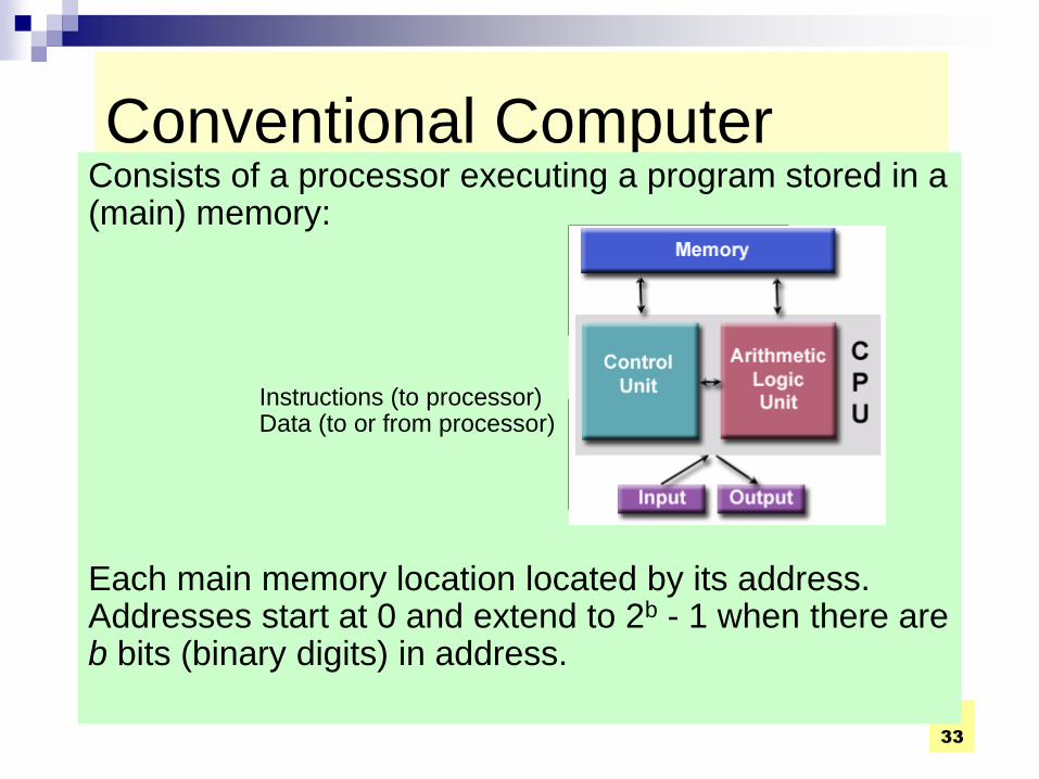
Conventional Computer Consists of a processor executing a program stored in a (main) memory:

Each main memory location located by its address. Addresses start at 0 and extend to 2b - 1 when there are b bits (binary digits) in address.

Main memory

Processor

Instr uctions (to processor) Data (to or from processor)

34

Shared Memory Multiprocessor System Natural way to extend single processor model - have multiple processors connected to multiple memory modules, such that each processor can access any memory module :

Processors

Interconnection network

Memory module One address space

35

Simplistic view of a small shared memory

multiprocessor

Examples:

Dual Pentiums

Quad Pentiums

Processors Shared memory

Bus

36

Quad Pentium Shared Memory

Multiprocessor

Processor

L2 Cache

Bus interface

L1 cache

Processor

L2 Cache

Bus interface

L1 cache

Processor

L2 Cache

Bus interface

L1 cache

Processor

L2 Cache

Bus interface

L1 cache

Memory controller

Memory

I/O interf ace

I/O b us

Processor/ memory b us

Shared memory

37

Programming Shared Memory

Multiprocessors

Threads - programmer decomposes program into individual

parallel sequences, (threads), each being able to access

variables declared outside threads.

Example: Pthreads (unix)

Sequential programming language with preprocessor

compiler directives to declare shared variables and specify

parallelism.

Example: OpenMP (needs OpenMP compiler)

38

Sequential programming language with added syntax to declare shared variables and specify parallelism.

Example UPC (Unified Parallel C) - needs a UPC compiler.

Parallel programming language with syntax to express parallelism - compiler creates executable code for each processor (not now common)

Sequential programming language and ask parallelizing compiler to convert it into parallel executable code. (not now common)

39

Message-Passing Multicomputer

Complete computers connected through an

interconnection network:

Processor

Interconnection network

Local

Computers

Messages

memory

40

Interconnection Networks

Limited and exhaustive interconnections

2- and 3-dimensional meshes

Hypercube (not now common)

Using Switches:

Crossbar

Trees

Multistage interconnection networks

Peer-to-peer

41

Two-dimensional array (mesh)

Links

Computer/

processor

42

Three-dimensional hypercube

000 001

010 011

100

110

101

111

In a d-dim hypercube, each node connects to one node in each dimension. Above a 3-d hypercube is shown. Each node is assigned a 3 bit address. Address difference between nodes is only 1 bit.

43

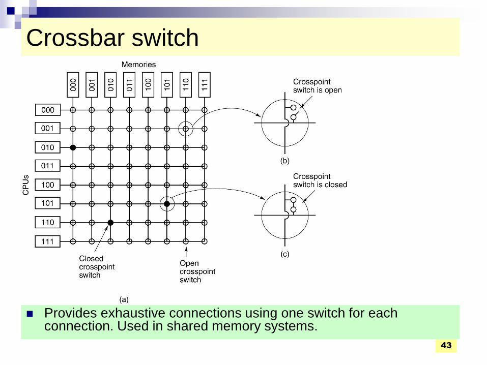
Crossbar switch

Provides exhaustive connections using one switch for each connection. Used in shared memory systems.

44

Tree

Switch element

Root

Links

Processors

45

Multistage Interconnection Network Example: Omega network

46

Communication Methods

Circuit switching Establish the path

Maintain/Reserve links for message passing

Simple telephone system is an example

Used in early multicomputers (INTEL IPSC-2)

Packet switching Divide message into “packets”

Packet = Source/Dest addresses + Data

Packet max size is known

Mail system is an example

47

Flynn’s Classifications

Flynn (1966) created a classification for computers based upon instruction streams and data streams:

Single instruction -single data (SISD) computer

Single processor computer - single stream of instructions generated from program. Instructions operate upon a single stream of data items.

48

Single Instruction, Single Data

(SISD):

• A serial (non-parallel) computer

• Single instruction: only one instruction stream is being acted on by the CPU during any one clock cycle

• Single data: only one data stream is being used as input during any one clock cycle

• Deterministic execution

• This is the oldest and until recently, the most prevalent form of computer

• Examples: most PCs, single CPU workstations and mainframes

49

SISD

50

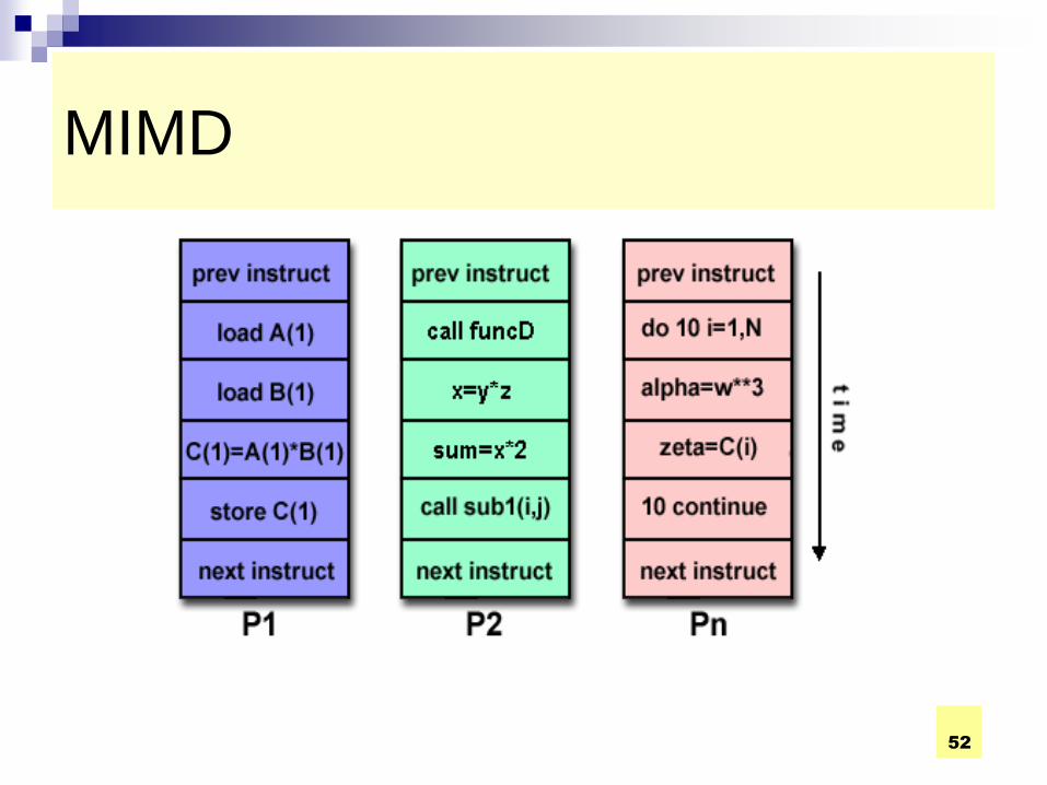
Multiple Instruction Stream-Multiple

Data Stream (MIMD) Computer

General-purpose multiprocessor system - each

processor has a separate program and one

instruction stream is generated from each program

for each processor. Each instruction operates

upon different data.

Both the shared memory and the message-

passing multiprocessors so far described are in the

MIMD classification.

51

MIMD

Multiple Instruction, Multiple Data (MIMD):

Currently, the most common type of parallel computer. Most modern computers fall into this category.

Multiple Instruction: every processor may be executing a different instruction stream

Multiple Data: every processor may be working with a different data stream

Examples: most current supercomputers, networked parallel computer "grids" and multi-processor SMP computers - including some types of PCs.

52

MIMD

53

Single Instruction Stream-Multiple Data

Stream (SIMD) Computer

A specially designed computer - a single instruction stream from a single program, but multiple data streams exist. Instructions from program broadcast to more than one processor. Each processor executes same instruction in synchronism, but using different data.

Developed because a number of important applications that mostly operate upon arrays of data.

COMPE472 Parallel Computing 54

SIMD Single Instruction, Multiple Data (SIMD):

A type of parallel computer

Single instruction: All processing units execute the same instruction at any given clock cycle

Multiple data: Each processing unit can operate on a different data element

This type of machine typically has an instruction dispatcher, a very high-bandwidth internal network, and a very large array of very small-capacity instruction units.

Best suited for specialized problems characterized by a high degree of regularity,such as image processing.

COMPE472 Parallel Computing 55

SIMD

56

Networked Computers as a Computing

Platform

A network of computers became a very attractive alternative to expensive supercomputers and parallel computer systems for high-performance computing in early 1990’s.

Several early projects. Notable:

Berkeley NOW (network of workstations) project.

NASA Beowulf project.

COMPE472 Parallel Computing 57

Key advantages:

Very high performance workstations and PCs

readily available at low cost.

The latest processors can easily be incorporated

into the system as they become available.

Existing software can be used or modified.

58

Software Tools for Clusters

Based upon Message Passing Parallel Programming:

Parallel Virtual Machine (PVM) - developed in late 1980’s. Became very popular.

Message-Passing Interface (MPI) - standard defined in 1990s.

Both provide a set of user-level libraries for message passing. Use with regular programming languages (C, C++, ...).

59

Beowulf Clusters*

A group of interconnected “commodity” computers achieving high performance with low cost.

Typically using commodity interconnects - high speed Ethernet, and Linux OS.

* Beowulf comes from name given by NASA Goddard Space Flight Center cluster project.

60

Cluster Interconnects

Originally fast Ethernet on low cost clusters

Gigabit Ethernet - easy upgrade path

More Specialized/Higher Performance Myrinet - 2.4 Gbits/sec - disadvantage: single vendor

cLan

SCI (Scalable Coherent Interface)

QNet

Infiniband - may be important as infininband interfaces may be integrated on next generation PCs