Asset Pricing - Constrained by Past Consumption Decisionsrepec.org/sce2004/up.23407.1076778817.pdf · ASSET PRICING and DYNAMIC PROGRAMMING 2 1 Introduction Intertemporal asset pricing

Asset Pricing -

Constrained by Past Consumption Decisions ∗

Lars Grune

Mathematisches Institut

Fakultat fur Mathematik und Physik

Universitat Bayreuth

95440 Bayreuth, Germany

[email protected]

Willi Semmler

Center for Empirical Macroeconomics

Bielefeld and

New School University, New York

[email protected]

July 1, 2004

Abstract: The attempt to match asset price characteristics such as the risk-free interest rate,equity premium and the Sharpe ratio with data for models with instantaneous consumption de-cisions and time separable preferences has not been very successful. Many recent versions ofasset pricing models have, in order to match those financial characteristics better with the data,employed habit formation where past consumption acts as a constraint on current consumption.In those models, surplus consumption, consumption over and above past consumption, improveswelfare, yet habit formation gives rise to an additional state variable. By studying such a modelwe also allow for adjustment costs of investment. The asset price characteristics that one obtainsfrom those models may depend on the solution techniques employed. In this paper a stochasticversion of a dynamic programming method with adaptive grid scheme is applied to compute theabove mentioned asset price characteristics where past consumption decisions are treated as anadditional state variable. Since, as shown in Grune and Semmler (2004), our method producesonly negligible errors it is suitable to be used as solution technique for such models with morecomplicated decision structure. Using our solution methods shows that there are still remainingpuzzles for the consumption based asset pricing model.

JEL Classification: C60, C61, C63, D90, G12

Keywords: stochastic growth models, habit formation, stochastic dynamic program-ming, adaptive grid, asset pricing

∗We want to thank Martin Lettau and Buz Brock for helpful communications.

1

ASSET PRICING and DYNAMIC PROGRAMMING 2

1 Introduction

Intertemporal asset pricing models with time separable preferences, such as power utilityor log utility, have been shown to have difficulties to match financial market characteristicssuch as risk-free interest rate, equity premium and the Sharpe-ratio, a measure of the risk-return trade off. In those models the risk-free interest rate turns out to be too high (andtoo smooth) and the mean equity premium and Sharpe-ratio too low as compared to whatone finds in time series data.

The conjecture has been that the solution methods to solve the optimal consumption pathin feedback form and to use the growth of marginal utility of consumption as discountfactor for pricing assets have been insufficient. Thus, one needs to be concerned with theaccuracy of the solution method to solve the model. One conjecture in the literature wasthus that the solution of stochastic growth models through linearizations for cases withmore complicated decision structure may not be appropriate. Recently, global solutiontechniques to the Hamilton-Jacobi-Bellman equation have been developed that can ad-dress this concern. A global solution method that is useful in this context is stochasticdynamic programming with discretization of the state space and adaptive gridding strat-egy which generates quite accurate solutions.1 A full discussion of the literature on thisand other methods is given in sect. 2.

Another concern has been that asset pricing models have often used models with exogenousdividend stream2 and the difficulties to match stylized financial statistics may have comefrom the fact that consumption is not endogenized. There is a tradition of asset pricingmodels that is based on the stochastic growth model with production originating in Brockand Mirman (1972) and Brock (1979, 1982) which endogenizes consumption. The Brockapproach extends the asset pricing strategy beyond endowment economies to economiesthat have endogenous state variables including capital stocks that are used in production.Authors, building on this tradition,3 have argued that it is crucial how consumptionis endogenized. In stochastic growth models the randomness occurs to the productionfunction of firms and consumption and dividends are derived endogenously. Yet, modelswith production have turned out to be even less successful. Given a production shock,consumption can be smoothed through savings and thus asset market features are evenharder to match.4

Recent development of asset pricing studies has therefore turned to extensions of in-tertemporal models conjecturing that the difficulties to match real and financial timeseries characteristics may be related to the simple structure of the basic model. In orderto match better asset price characteristics of the model to the data economic researchhas extended the baseline stochastic growth model to include different utility functions,

1For deterministic versions, see Grune (1997), Santos and Vigo–Aguiar (1998), and Grune and Semmler(2004).

2Those models originate in Lucas (1978) and Breeden (1979) for example.3See Rouwenhorst (1995, Akdeniz and Dechert (1997), Jerman (1998), Boldrin, Christiano and Fisher(2001), Lettau and Uhlig (1999) and Hansen and Sargent (2002), the latter in a linear-quadratic economy.The Brock model has also been used to evaluate the effect of corporate income tax on asset prices, seeMcGrattan and Prescott (2001).

4For a recent account of the gap between models and facts, see Boldrin, Christiano and Fisher (2001),Cochrane (2001, ch. 21), Lettau, Gong and Semmler (2001) and Semmler (2003, chs. 9-10).


in particular habit formation, adjustment costs of investment, idiosyncratic technologyshocks to firms or the effect of leverage on firm value.5 In this paper we will focus on anintertemporal decision model with habit formation and adjustment costs of investment.

Since, as aforementioned, time separable preferences fail to match financial market char-acteristics an enormous effort has been invested into models with time non-separablepreferences, such as habit formation models, which allow for adjacent complementarity inconsumption. Past consumption enters here as a constraint, defined as external habit per-sistence where the aggregate level of consumption serves as a benchmark level, or internalhabit persistence where a household’s own past consumption is viewed as a benchmarkover and above welfare is considered to be increasing. If one chooses internal habit per-sistence, given by past consumption, as benchmark, it is then in general time varying.

There is a long tradition in economic theory where it is assumed that habits are formedthrough past consumption.6 Habit persistence is nowadays used to understand a widerange of issues in growth theory (Carrol et al. 1997, 2000, Alvarez-Cuadrado et al. 2004)macroeconomics (Fuhrer, 2002), and business cycle theory (Boldrin et al, 2001). In all ofthose models of habit persistence high level of consumption in the past depresses currentwelfare and high current consumption depresses future welfare. This can be writtenas ratios of current over past consumption (Abel 1990, 1999) or in difference form as(1 − α)Ct + α(Ct − Ct−1) with Ct current, Ct−1 past consumption and α a respectiveweight. This form of habit formation will be chosen in this paper.

This type of habit specification gives rise to time non-separable preferences where riskaversion and intertemporal elasticity substitution are separated and a time variation ofrisk aversion will arise. If we define surplus consumption as st = Ct−Xt

Ctwith Xt, the

habit, and γ, the risk aversion parameter, then the time variation of risk-aversion is γst

:the risk aversion falls with rising surplus consumption and the reverse holds for fallingsurplus consumption. A high volatility of the surplus consumption will lead to a highvolatility of the growth of marginal utility and thus to a high volatility of the stochasticdiscount factor.

Habit persistence in asset pricing has been introduced by Constantinides (1990) in orderto account for high equity premia. Asset pricing models along this line have been furtherexplored by Campbell and Cochrane (1999), Jerman (1998), and Boldrin et al. (2001).Yet, asset pricing introducing habit persistence in stochastic models with production mayjust produce smoother consumption. But with income different from consumption, forexample due to shocks, habit formation amplifies investment and demand for capitalgoods. Yet, Boldrin et al. (2001) have argued if there is, however, perfectly elastic supplyof capital there is no effect on the volatility of the return on equity. As the literaturehas demonstrated (Jerman 1998, and Boldrin et al. 2001) one also needs adjustmentcosts of investment to minimize the elasticity of the supply of capital. It seems to be bothhabit persistence and adjustment costs for investment which are needed to generate higherequity premia. By choosing such a model we will not, following Jerman (1998), allow forelastic labor supply, but rather employ a model with fixed labor supply, since the latter,

5For further detailed studies of those extensions see, for example, Campbell and Cochrane (1999), Jerman(1998), Boldrin, Christiano and Fisher (2001) and Cochrane (2001, ch. 21).

6See the description in Marshall (1920), Veblen (1899) and Duesenberry (1949). For a first use of habitpersistence in a dynamic decision model see Ryder and Heal (1973).


as shown in Lettau and Uhlig (2000), provides the most favorable case for matching themodel with the financial market characteristics.

Since accuracy of the solution method is an intricate issue for models with more compli-cated decision structure, we first have to have sufficient confidence in the accuracy of thestochastic dynamic programming method that we will use. In our method we do not usefixed grids, but adaptive space discretization. In the method applied in our paper efficientand reliable local error estimation is undertaken and used as a basis for a local refinementof the grid in order to deal with regions of steep slopes or non-smooth properties of thevalue function (such as non-differentiability). This procedure allows for a global dynamicanalysis of deterministic as well as stochastic intertemporal decision problems.

In Grune and Semmler (2004) a stochastic dynamic programming algorithm with flexiblegrid size has been tested for the most basic stochastic growth model as based on Brockand Mirman (1972) and Brock (1979, 1982). This model can analytically be solved forthe sequence of optimal consumption in feedback form. Asset prices, the risk-free interestrate, the equity premium and the Sharpe-ratio, can, once the model is solved analyticallyfor the sequence of optimal consumption, easily be solved numerically and those solutionscan be compared to the numerical solutions obtained from our numerical procedure. Ashas been shown in Grune and Semmler (2004) the errors, as compared to the analyticalsolutions, are negligibly small. Thus, the method we employ here can confidently beapplied to extensions of the basic model with more complicated decision structure.

The paper is organized as follows. Section 2 discusses related literature. Section 3 presentsthe stochastic dynamic programming algorithm. Section 4 introduces our model of assetpricing with habit persistence and adjustment costs of investment and the measures ofthe financial characteristics we want to study. Section 5 reports the numerical results ofour study which are evaluated in section 6. Section 7 concludes the paper.

2 Related Literature on Solution Methods

In the literature on solving asset pricing models one can find a vast amount of differentapproaches most of them using linear approximations.7 The most promising approachesare those ones that are employing the dynamic programming approach since it is closelyrelated to the Hamilton-Jacobi-Bellman equation for asset pricing. Many of the recentversions of dynamic programming use state–of–the art mathematical and numerical tech-niques for making this approach more efficient. Here we apply an adaptive griddingalgorithm that works for very general Hamilton-Jacobi-Bellman equations, see Section 3for details. In the present section we briefly review similar approaches and highlightsimilarities and differences to our approach.

One of the fundamental difficulties with the dynamic programming approach is that thecomputational load grows exponentially with the dimension of the problem, a phenomenonknown as the “curse of dimensionality” (see Rust (1996) for a comprehensive account oncomplexity issues). In our case, for computing asset pricing in the context of stochasticgrowth models with habit formation the problem to be solved is three dimensional, hence

7For an extensive survey of those techniques, see Taylor and Uhlig (1990).


this is not a crucial aspect. Nevertheless, for the sake of completeness we want to mentionapproaches like randomly distributed grid points (Rust (1997)) or so called low discrepancygrids (Rust (1996), Reiter (1999)) which are able to break the curse of dimensionality. Inprinciple also Monte–Carlo techniques like in Keane and Wolpin (1994) allow for breakingthe curse of dimensionality, but as Rust (1997) points out, the specific algorithm in Keaneand Wolpin (1994) uses an interpolation technique which again is subject to exponentialgrowth of the numerical cost in the space dimension.

For low dimensional problems the goal of the numerical strategy is not to avoid the curseof dimensionality but rather to reduce the computational cost for a problem of fixeddimension. For this purpose, two main approaches can be found in the literature, namelyhigher order approximations and adaptive gridding techniques; the latter will be used inour numerical approach.

The idea of high order approximations lies in exploiting the smoothness of the optimalvalue function: if the optimal value function turns out to be sufficiently smooth, thenmethods using approximations by smooth functions, like Chebyshev polynomials (Rust(1996), Judd (1996), Jermann (1998)), Splines (Daniel (1976), Johnson et al. (1993),Trick and Zin (1993, 1997)) or piecewise high–order approximations (Falcone and Ferretti(1998)) can be very efficient. Smoothness is also the basis of other high–order strategies,like in finite difference approximations (Candler (2001)), Gaussian Quadrature discretiza-tion (Tauchen and Hussey (1991), Burnside (2001)) and in perturbation techniques (Judd(1996)). Yet, the last should also work if the value function is only piecewise smooth.8

Some of these methods (like Spline and piecewise high order approximation) use a (fixed)grid discretization of the state space similar to our approach. The combination of adaptivegrids with higher order approximation is currently under investigation and it will beinteresting to see whether adaptive discretization ideas based on our local error estimationtechnique work equally well with these approximation techniques.

Concerning discretization techniques it should be noted that from the complexity point ofview it turns out to be optimal to solve the dynamic programming problem on successivelyfiner grids, using a one–way multigrid strategy (Chow and Tsitsiklis (1991), see alsoRust (1996)). In fact, our adaptive gridding algorithm is similar to this approach sincethe approximation on the previous grid Γi is always used as the initial value for thecomputation on the next finer adaptive grid Γi+1. This also explains the large reductionin computation time observed for our approach compared to the computation on one fixedequidistant grid.

Let us now turn to the methodology employed here, i.e., adaptive gridding techniques.Perhaps closest to our approach are the techniques discussed in Munos and Moore (2002).Here a number of heuristic techniques are compared which lead to local and global errorindicators which can in turn be used for an adaptive grid generation. Some of the in-dicators discussed in this paper bear some similarity with our residual based estimator,though rigorous estimates as employed in out method, below, are not given there. In anycase, the authors report that these techniques are unsatisfactory and argue for a com-pletely different approach which measures the influence of local errors in certain regions

8For an early survey of those methods, see Taylor and Uhlig (1990) where one can find a comparativenumerical study of several methods.


on the global error by analyzing the information flow on the Markov chain related to thediscretization of the (deterministic) problem at hand. The reason for this lies in the factthat the model problem treated by Munos and Moore (2002) has a discontinuous optimalvalue function, which often happens in technical problems with boundary conditions. Infact, also our adaptive scheme performs rather poorly in presence of discontinuities butsince our economic problems do always have continuous optimal value functions, Munos’and Moore’s conclusions do not apply here. A roughly similar technique is the endogenousoversampling used by Marcet (1994). This is again a heuristic method, which, however,does not lead to adaptive grids but rather selects suitable parts of the state space wherethe optimally controlled trajectories stay with high probability.

Probably the adaptive approaches with the most solid mathematical background are pre-sented in the papers of Trick and Zin (1993, 1997).9 In these papers an alternativeapproach for the solution of the fully discrete problem is developed using advanced linearprogramming techniques which are capable of solving huge linear programs with manyunknowns and constraints. In Trick and Zin (1993) an adaptive selection of constraintsin the linear program is used based on estimating the impact of the missing constraint, amethod which is closely related to the chosen solution method but only loosely connectedto our adaptive gridding approach. The later paper (Trick and Zin (1997)), however,presents an idea which is very similar to our approach. Due to the structure of theirsolution they can ensure that the numerical approximation is greater than or equal to thetrue optimal value function. On the other hand, the induced suboptimal optimal controlstrategy always produces a value which is lower than the optimal value. Thus, comparingthese values for each test point in space one can compute an interval in which the truevalue must lie, which produces a mathematically concise error estimate that can be usedas a refinement criterion. While this approach is certainly a good way to measure errors,which could in particular be less conservative than our measure for an upper bound, westrongly believe that it is less efficient for an adaptive gridding scheme, because (i) theestimated error measured by this procedure is not a local quantity (since it depends onthe numerical along the whole suboptimal trajectory), which means that regions may berefined although the real error is large elsewhere, and (ii) compared to our approach it isexpensive to evaluate, because for any test point one has to compute the whole suboptimaltrajectory, while our residual based error estimate needs only one step of this trajectory.

Let us comment on the idea of a posteriori error estimation. In fact, the idea to evaluateresiduals can also be found in the papers of Judd (1996) and Judd and Guu (1997), using,however, not the dynamic programming operator but the associated Euler equation. Inthese references the resulting residual was used to estimate the quality of the approxi-mating solution, but to our knowledge it has not been used to control adaptive griddingstrategies, and we are not aware of any estimates such as ours which is a crucial prop-erty for an efficient and reliable adaptive gridding scheme, particularly needed to solvestochastic problems in asset pricing models.

Summarizing our discussion, there are a number of adaptive strategies around which areall reported to show good results, however, they are either heuristic10 and better suited for9As mentioned above, this approach also uses splines, i.e., a smooth approximation, but the ideas developedin these papers do also work for linear splines which do not require smoothness of the approximatedoptimal value function.

10In order to avoid misunderstandings: We do not claim that heuristic methods cannot perform well; in


other classes of problems than asset pricing models or they have nice theoretical featuresbut are practically inconvenient because their implementation is numerically much moreexpensive than our approach.

3 Stochastic Dynamic Programming

Next we describe the stochastic dynamic programming algorithm that we use to solve theasset pricing characteristics of the intertemporal decision we want to study. Our approachis characterized by using a combined value function and policy iteration and permittinggrid refinements due to error estimates.

We consider the discrete stochastic dynamic programming equation

V (x) = maxc∈C

Eu(x, c, ε) + β(x, ε)V (ϕ(x, c, ε)). (3.1)

Here x ∈ Ω ⊂ R3, C ⊂ R, Ω and C are compact sets and ε is a random variable withvalues in R . The mappings ϕ : Ω × C × R → R3 and g : Ω × C × R → R are supposedto be continuous and Lipschitz continuous in x. Furthermore, we assume that eitherϕ(x, c, z) ∈ Ω almost surely for all x ∈ Ω and all c ∈ C , or that suitable boundaryvalues V (x) for x 6∈ Ω are specified, such that the right hand side of (3.1) is well definedfor all x ∈ Ω. The value β(x, ε) is the (possibly state and ε dependent) discount factorwhich we assume to be Lipschitz and we assume that there exists β0 ∈ (0, 1) such thatβ(x, ε) ∈ (0, β0) holds for all x ∈ Ω. We can relax this condition if no maximization takesplace, in this case it suffices that all trajectories end up in a region where β(x, ε) ∈ (0, β0)holds. This is the situation for the asset price problem, cf. the discussion in Cochrane(2001:27).

Associated to (3.1) we define the dynamic programming operator

T : C(Ω, R) → C(Ω, R)

given byT (W )(x) := max

c∈CEu(x, c, ε) + β(x, ε)W (ϕ(x, c, ε)). (3.2)

The solution V of (3.1) is then the unique fixed point of (3.2), i.e.,

T (V ) = V. (3.3)

For the numerical solution of (3.3) we use a discretization method that goes back toFalcone (1987) and in Santos and Vigo–Aguiar (1998) in the deterministic case. Here weuse unstructured cuboidal grids: We assume that Ω ⊂ R3 is a cuboid and consider a gridΓ covering Ω with cuboidal elements Ql and nodes xj and the space of continuous andpiecewise multilinear functions

WΓ := W ∈ C(Ω, R) |W (x + αej) is linear in α on each Ql for each j = 1, 2, 3

fact they can show very good results. Our main concern about these methods is that one can never besure about the quality of the final solution of a heuristic method.


where the ej , j = 1, 2, 3 denote the standard basis vectors of the R3, see Grune (2004) fordetails of the grid construction. With πΓ : C(Ω, R) →WΓ we denote the projection of anarbitrary continuous function to WΓ, i.e.,

πΓ(W )(xj) = W (xj) for all nodes xj of the grid Γ.

Note that our approach easily carries over to higher order approximations, the use of mul-tilinear approximations is mainly motivated by its ease of implementation, especially foradaptively refined grids.11 Also, the approach can easily be extended to higher dimensions.

We now define the discrete dynamic programming operator by

TΓ : C(Ω, R) →WΓ, TΓ = πΓ T (3.4)

with T from (3.2). Then the discrete fixed point equation

TΓ(VΓ) = VΓ. (3.5)

has a unique solution VΓ ∈ WΓ which converges to V if the size of the elements Ql tends tozero. The convergence is linear if V is Lipschitz on Ω, see Falcone (1987), and quadraticif V is C2, see Santos and Vigo–Aguiar (1998).

For the solution of (3.5) we need to evaluate the operator TΓ. More precisely, we need toevaluate

maxc∈C

Eu(xj , c, ε) + β(xj , ε)W (ϕ(xj , c, ε)).

for all nodes xj of Γ.

This first includes the numerical evaluation of the expectation E. If ε is a finite ran-dom variable then this is straightforward, if ε is a continuous random variable then thecorresponding integral ∫

(u(x, c, ε) + β(x, ε)V (ϕ(x, c, ε)))f(ε)dε

has to be computed, where f is the probability density of ε. In our implementation weapproximated this integral by a trapezoidal rule with 10 equidistant intervals.

The second difficulty in the numerical evaluation of T lies in the maximization over c.In our implementation we used a recursive discrete approximation of the feasible valuesin the set C, i.e., of those values c ∈ C for which u(x, c, ε) is defined. The maximumis approximated by comparing finitely many values in C, then a neighborhood of thiscandidate is refined to obtain a new approximate maximum, a procedure which is repeatedrecusrively for several times. It can be shown that for unimodal functions this procedureindeed converges to the maximum and even though for our functions this property cannotbe shown rigorously this procedure shows very good results in practice.

For the solution of the fixed point equation (3.5) we use the Gauss–Seidel type value spaceiteration where we subsequently compute Vi+1 = SΓ(Vi) with SΓ being a Gauss–Seideltype iteration operator (including the maximization over c ) obtained from TΓ. Thisiteration is coupled with a policy space iteration: Once a prescribed percentage of the11The combination of adaptive grids and higher order approximations is currently under investigation.


maximizing u–values in the nodes remains constant from one iteration to another we fixall control values and compute the associated value function by solving a linear system ofequations using the iterative CGS method. After convergence of this method we continuewith the value space iteration using SΓ until the control values again converge, switch tothe linear solver and so on. This combined policy–value space iteration turns out to bemuch more efficient (often more than 90 percent faster) than the plain Gauss–Seidel valuespace iteration using SΓ

12 The details of the adaptive gridding strategy based on errorestimates are presented in the appendix.

4 The Stochastic Decision Problem in Asset Pricing

Our stochastic decision problem arising from the stochastic growth model in the Brocktradition which we want to solve and for which we want to compute certain financialmeasures is as follows. Before we introduce the baseline stochastic growth model that wewant to apply our solution technique too, see sect. 5, we outline an asset pricing modelin a very generic form. The problem we are concerned with is to solve an optimal control,ct, for the dynamic decision problem

V (k, z) = maxct

E

( ∞∑t=0

βiu(ct, Xt)

)(4.1)

with habit Xt, subject to the dynamics

kt+1 = ϕ1(kt, zt, ct, εt)zt+1 = ϕ2(kt, zt, ct, εt)

Xt+1 = ct

using the constraints ct ≥ 0 and kt ≥ 0 and the initial value k0 = k, z0 = z, X0 = X.Here (kt, zt, Xt) ∈ R3 is the state and εt are i.i.d. random variables. We abbreviatext = (kt, zt, Xt) and ϕ(x, c, ε) = (ϕ1(k, z, c, ε), ϕ2(k, z, c, ε), ct), i.e.,

xt+1 = ϕ(xt, ct, εt). (4.2)

This optimal decision problem allows for the computation of c in feedback form, i.e.ct = c(xt) for a map c : R3 → R. Based on this c we compute the stochastic discountfactor13

m(xt) = βu′(c(xt+1), Xt)u′(c(xt), Xt)

(4.3)

(note that m depends on εt and the derivative u′ is taken with respect to ct), which servesas an ingredient for the next step, which consists of solving the asset pricing problem

p(x) = E

( ∞∑t=1

t∏s=1

m(xs)d(xt)

), (4.4)

12The latter in turn is considerably faster than the Banach iteration Vi+1 = TΓ(Vi).13The following financial measures are introduced and studied in detail in Cochrane (2001).


where d(xt) denotes the dividend at xt and x0 = x and the dynamics are given by

xt+1 = ϕ(xt, c(xt), εt)

with c from above.

Finally, we use these values to compute the Sharpe ratio, which represents the ratio ofthe equity premium to the standard deviation of the equity return.

S =∣∣∣∣E(R(x))−Rf (x)

σ(R(x))

∣∣∣∣ = −Rf (x)cov(m(x), R(x)

)σ(R(x))

. (4.5)

In this formulaRf (x) =

1E(m(x))

(4.6)

is the risk-free interest rate and

R(xt) =d(xt+1) + p(xt+1)

p(xt)(4.7)

is the gross return.

Note that the equality E(m(x)R(x)) = 1 holds, which can serve as a indicator for theaccuracy of our numerical solution.

We solve the asset pricing problem in the following three steps: (i) We compute theoptimal value function V of the underlying optimal control problem, and compute c fromV , (ii) we compute the prices p(x) from c and m, and (iii) we compute the risk-free interestrate, the equitiy premium and the Sharpe ratio S from c, m and p.

For a baseline stochastic growth model without habit formation both c and p are actuallyavailable analytically. This has been used for extensive accuracy tests of our algorithm,see Grune and Semmler (2004).

For each of the steps we do now sketch our technique for the numerical computation usingthe algorithm described above in Section 3.

Step (i):

For the solution of the optimal control problem we use the dynamic programming al-gorithm with adaptive grid. In order to solve (4.1) we solve the equivalent dynamicprogramming equation (3.1), i.e.,

V (x) = maxc

E (u(c) + βV (ϕ(x, c, ε))) =: T (V )(x)

using the algorithm described in sect. 3 which gives a numerical approximation VΓ of V .

Once VΓ is computed with sufficient accuracy we can obtain the optimal control value c(x)in each point by choosing c(x) such that (3.1) — with VΓ instead of V — is maximized,i.e., such that

E (u(c(x)) + βVΓ(ϕ(x, c(x), ε))) = maxc

E (u(c) + βVΓ(ϕ(x, c, ε)))

holds. Once c is known, m of equ. (4.3) can be computed from this value.


Step (ii):

For computing p(x) we follow the same approach as in Step (i), except that here c(x) isknown in advance and hence no maximization needs to be done.

For the computation of p we first solve the dynamic programming equation

p(x) = E(d(x) + m(x)p(ϕ(x, c(x), ε)))

which is simply a system of linear equations which we solve using the CGS method. Thisyields a numerical approximation of the function

p(x) = E

( ∞∑t=0

t∏s=1

m(xs)d(xt)

)

(with the convention∏0

s=1 m(xs) = 1), from which we obtain p by

p(x) = p(x)− d(x).

In our numerical computations for the computation of p we have always used the samegrid Γ as in the previous computation of V in Step (i). The reason is that it did not seemjustified to use a finer grid here, because the accuracy of the entering values c from Step(i) is limited by the resolution of Γ, anyway. However, it might nevertheless be that usinga different grid (generated e.g. by an additional adaptation routine) in Step (ii) couldincrease the numerical accuracy.

Step (iii):

The last step is in principle straightforward, because we do now have all the necessaryingredients to compute the risk-free interest rate, the equity premium and Sharpe ratio Sand its upper bound SB. However, since all the numerical values entering these computa-tions are subject to numerical errors we have to be concerned with the numerical stabilityof the respective magnitudes. The first formula for the Sharpe ratio, where the numeratorrepresents the equity premium, as the spread between the expected equity return and therisk-free interest rate, ∣∣∣∣E(R(x))−Rf (x)

σ(R(x))

∣∣∣∣ . (4.8)

turns out to be considerably less precise than the second formula

−Rf (x)cov(m(x), R(x)

)σ(R(x))

. (4.9)

Since the denominator is the same in both formulas, the difference can only be caused bythe different numerators. A further investigation reveals that the numerator of the firstformula can be rewritten as

Rf (x)(1− E(m(x))E(R(x)))

while that of the second formula reads

Rf (x)(E(m(x)R(x))− E(m(x))E(R(x))).


Note that in both formulas we have to subtract values which have approximately the samevalues, which considerably amplifies the numerical errors. As mentioned above, we knowthat E(m(x)R(x)) = 1, which shows that these formulas are theoretically equivalent. Yetthe second formula is more accurate.14

5 Numerical results

We have applied our numerical scheme to the model given by

kt+1 = ϕ1(kt, zt, ct, εt) = kt +kt

1− ϕ

[(It

kt

)1−ϕ

− 1

]

ln zt = ϕ2(kt, zt, ct, εt) = ρ ln zt + εt,

with It = ztAkαt − ct, where in our numerical computations we used the variable yt = ln zt

instead of zt as the second variable.

The utility function is given by

u(ct, Xt) =(ct − bXt)1−γ − 1

1− γ

for γ 6= 1 and byu(ct, Xt) = ln(ct − bXt)

for γ = 1. Since we are working with internal habit, in our case, we have Xt = Ct−1.

For our numerical experiments we employed the values

A = 5, α = 0.34, ρ = 0.9, β = 0.95, b = 0.5

and εt was chosen as a Gaussian distributed random variable with standard deviation σ =0.008, which we restricted to the interval [−0.032, 0.032]. With this choice of parametersit is easily seen that the interval [−0.32, 0.32] is invariant for the second variable yt.14The higher accuracy of the second formula can be explained as follows: Assume that we have a small

systematic additive numerical error in R(x), e.g., Rnum(x) ≈ R(x) + δ. Such errors are likely to becaused by the interpolation process on the grid. Then, using Rf (x) = 1/E(m(x)), in the first formulawe obtain

Rf (x)(1− E(m(x))E(Rnum(x))) ≈ Rf (x)(1− E(m(x))E(R(x) + δ))

≈ Rf (x)(1− E(m(x))E(R(x)))− δ,

while in the second formula we obtain

Rf (x)(E(m(x)Rnum(x))− E(m(x))E(Rnum(x)))

≈ Rf (x)(E(m(x)(R(x) + δ))− E(m(x))E(R(x) + δ))

≈ Rf (x)(E(m(x)R(x)) + E(m(x))δ − E(m(x))E(R(x))− E(m(x))δ)

≈ Rf (x)(E(m(x)(R(x)))− E(m(x))E(R(x))),

i.e., systematic additive errors cancel out in the second formula.


Motivated by our 2d studies (Grune and Semmler (2004)) we would like to solve ourproblem for kt in the interval [0.1, 10]. However, the habit persistence implies that fora given habit Xt only those value ct are admissible for which ct − bXt > 0 holds, whichdefines a constraint from below on ct depending on the habit Xt. On the other hand, thecondition It ≥ 0 defines a constraint from above on ct depending on kt and yt = ln zt. Asa consequence, there exist states xt = (kt, yt, Xt) for which the set of admissible controlvalues ct is empty, i.e., for which the problem is not feasible. On the one hand, we wantto exclude these points from our computation, on the other hand we want to have acomputational domain which is of a simple shape. A solution for this problem is given bya coordinate transformation which transforms a suitable set Ω of feasible points to the setΩ = [0.1, 10]× [−0.32, 0.32]× [0, 7] on which we perform our computation. The coordinatetransformation Ψ : R3 → R3 we use for this purpose shifts the k–component of a pointx = (k, y,X) in such a way that any non–feasible point x is mapped to a point x 6∈ Ω. Itis given by

Ψ(k, y,X) := (k − s(y, X), y,X)

with

s(y, X) =(

s0 + bX

exp(y)A

) 1α

− 0.1

where s0 = 0.1α exp(−0.32)A is chosen such that for y = −0.32 and X = 0 the coordinatechange is the identity. This map is built in such a way that for all points xt ∈ Ω =Ψ−1(Ω) a value ct with ct − bXt ≥ s0 is admissible. Note that forward invariance of Ωis not automatically guaranteed by this construction but it turned out to hold for all theparameter values we used in the tests described below.

This coordinate transformation allows us to set up our dynamic programming algorithmon a set of feasible points without having to deal with a complicated domain Ω, becausenumerically we can now work on the simple set Ω using the transformed dynamics

xt+1 = Ψ ϕ(Ψ−1(xt), ct, εt)

instead of (4.2). For the graphical output, below, the results were re–transformed to theoriginal coordinates.

In all our computations we have used the adaptive gridding algorithm described in theappendix with θ = 0.1 and tol = 10−4, using final grids with ≈ 100000 nodes.

In addition to the parameters specified above, for our numerical experiments we have usedthe following sets of parameters:

(a) ϕ = 0, γ = 1, b = 0

(b) ϕ = 0, γ = 1, b = 0.5

(c) ϕ = 0, γ = 3, b = 0.5

(d) ϕ = 0.8, γ = 1, b = 0.5

(e) ϕ = 0.8, γ = 3, b = 0.5


Note that (a) corresponds to the setting from Grune and Semmler (2004) for which theanalytical solution is available.

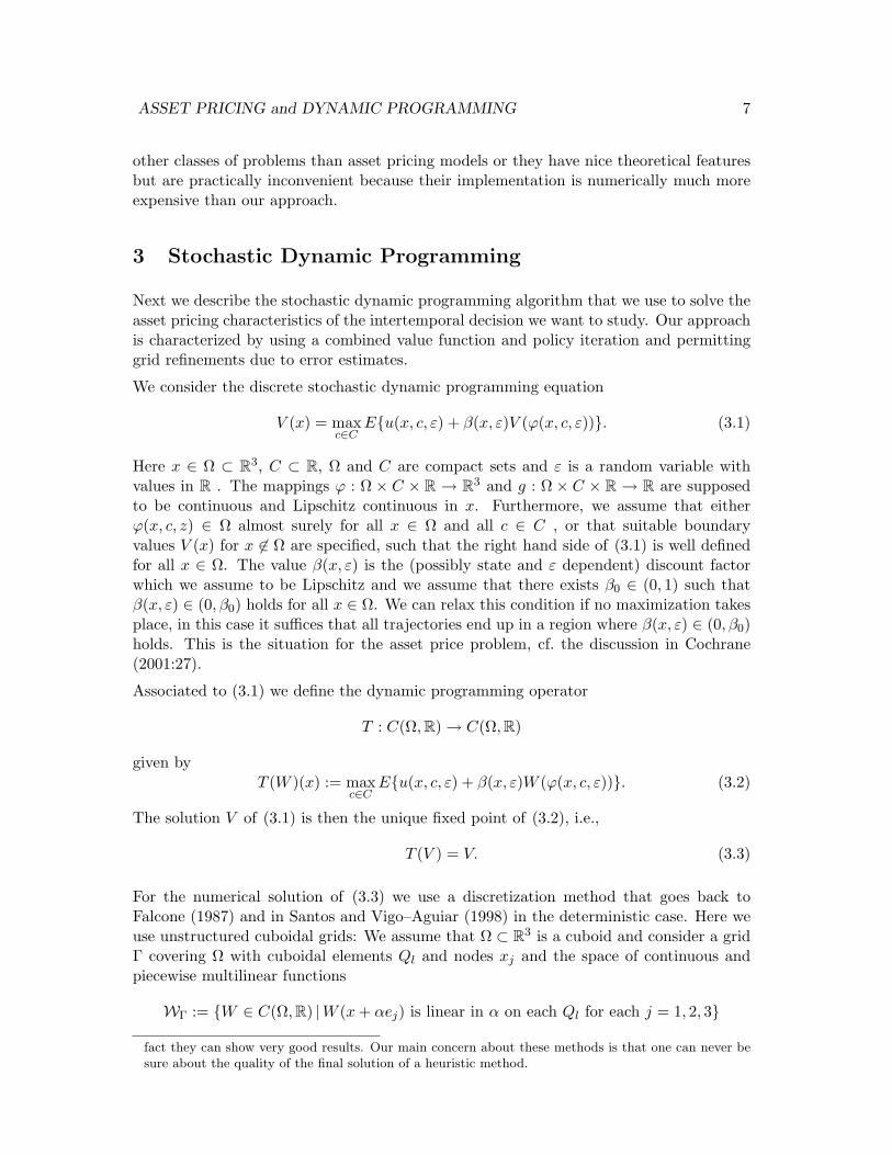
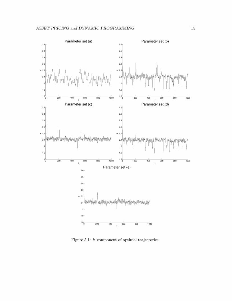
Our first set of numerical results shows the behavior of the kt–component of the optimaltrajectories of the optimal control problem (4.1) in Figure 5.1 (a)–(e), the stochasticdiscount factor along these trajectories in Figure 5.2(a)–(e) and the consumption in Figure5.3(a)–(e). For all trajectories we used the initial value (k0, y0, X0) = (2, 0, 4) which is nearthe point around which the optimal trajectory oscillates. Furthermore, for all trajectorieswe have used the same sequence of the random variables εt.


0 200 400 600 800 10001.8

1.9

2

2.1

2.2

2.3

2.4

2.5

2.6Parameter set (a)

t

k

0 200 400 600 800 10001.8

1.9

2

2.1

2.2

2.3

2.4

2.5

2.6Parameter set (b)

t

k

0 200 400 600 800 10001.8

1.9

2

2.1

2.2

2.3

2.4

2.5

2.6Parameter set (c)

t

k

0 200 400 600 800 10001.8

1.9

2

2.1

2.2

2.3

2.4

2.5

2.6Parameter set (d)

t

k

0 200 400 600 800 10001.8

1.9

2

2.1

2.2

2.3

2.4

2.5

2.6Parameter set (e)

t

k

Figure 5.1: k–component of optimal trajectories


0 200 400 600 800 10000.7

0.8

0.9

1

1.1

1.2

t

βParameter set (a)

0 200 400 600 800 10000.7

0.8

0.9

1

1.1

1.2

t

β

Parameter set (b)

0 200 400 600 800 10000.7

0.8

0.9

1

1.1

1.2

t

β

Parameter set (c)

0 200 400 600 800 10000.7

0.8

0.9

1

1.1

1.2

t

β

Parameter set (d)

0 200 400 600 800 10000.7

0.8

0.9

1

1.1

1.2

t

β

Parameter set (e)

Figure 5.2: Stochastic discount factor β along optimal trajectories


0 200 400 600 800 10003.9

4

4.1

4.2

4.3

4.4

4.5

4.6

4.7

4.8

4.9

t

cParameter set (a)

0 200 400 600 800 10003.9

4

4.1

4.2

4.3

4.4

4.5

4.6

4.7

4.8

4.9

t

c

Parameter set (b)

0 200 400 600 800 10003.9

4

4.1

4.2

4.3

4.4

4.5

4.6

4.7

4.8

4.9

t

c

Parameter set (c)

0 200 400 600 800 10003.9

4

4.1

4.2

4.3

4.4

4.5

4.6

4.7

4.8

4.9

t

c

Parameter set (d)

0 200 400 600 800 10003.9

4

4.1

4.2

4.3

4.4

4.5

4.6

4.7

4.8

4.9

t

c

Parameter set (e)

Figure 5.3: Consumption c along optimal trajectories


The following Table 5.1 shows several characteristic values obtained from our algorithm.The values were obtained by averaging the values along the optimal trajectories depictedabove.

parameter set Sharpe ratio equity premium risk free interest rate

(a) 0.0085 0.00008 1.051(b) 0.0153 0.00021 1.049(c) 0.0540 0.00227 1.084(d) 0.0201 0.00031 1.060(e) 0.0572 0.00329 1.085

Table 5.1: Numerically computed values

As can be observed from the figures 5.2 (c) and (e) the stochastic discount factor is mostvolatile for the combination of a high γ and habit persistence, whereas habit persistence byitself increases the stochastic discount factor only moderately. Moreover, as the figures 5.3(a)-(b) show, the consumption path itself is only very little affected by habit persistenceand adjustment costs of capital.15 From the table 5.1 we can observe that the Sharperatio and equity premium increase strongly with habit persistence and adjustment costs,though not sufficiently to match empirical facts, but the risk free interest rate is still muchtoo high.

6 Interpretation of the Results

It is interesting to compare the numerical results that we have obtained, by using stochas-tic dynamic programming, to previous quantitative studies undertaken for habit forma-tion, but using other solution techniques. We in particular will restrict ourselves to acomparison with the results obtained by Boldrin et al. (2001) and Jerman (1998).

Whereas Boldrin et al. use a model with log utility for internal habit, but endogenouslabor supply in the household’s preferences, Jerman studies the asset price implication ofa stochastic growth model, also with internal habit formation but, as in our model, laboreffort is not a choice variable. All three papers Boldrin et al. (2001), Jerman (1998) andour variant use adjustment costs of investment in the model with habit formation. Bothprevious studies claim that habit formation models with adjustment costs can match thefinancial characteristics of the data. Yet, both studies have chosen parameters that appearto be conducive to results which replicate better the financial characteristics such as riskfree rate, equity premium and the Sharpe ratio.

In comparison to their parameter choice we have chosen parameters that have commonlybeen used for stochastic growth models16 and that seem to describe the first and secondmoments of the data well. Table 5.2 reports the parameters and the results.

15Note that our result on habit persistence is a result that Lettau and Uhlig (2000) have also predicted.16See Santos and Vigo-Aguiar (1998).


Both, the study by Boldrin et al. (2001) and Jerman (1998) have chosen a parameter,ϕ = 4.05, in the adjustment costs of investment, a very high value which is at the veryupper bound found in the data.17 Since the parameter ϕ smoothes the fluctuation of thecapital stock and makes the supply of capital very inelastic, we have rather worked with aϕ = 0.8 in order to avoid such strong volatility of returns generated by high ϕ. Moreover,both papers use a higher parameter for past consumption, b, than we have chosen. Bothpapers have also selected a higher standard deviation of the technology shock. Boldrin etal. take σ = 0.018, and Jerman takes a σ = 0.01, whereas we use σ = 0.008 which has beenemployed in many models.18 Those parameters increase the volatility of the stochasticdiscount factor, a crucial ingredient to raise the equity premium and the Sharpe ratio.

Boldrin et al.a) Jermanb) Grune US Datac)

and Semmler (1954-1990)

b= 0.73-0.9 b= 0.83 b= 0.5ϕ=4.15 ϕ=4.05 ϕ= 0.8σ= 0.018 σ= 0.01 σ= 0.008ρ= 0.9 ρ= 0.99 ρ= 0.9β= 0.999 β= 0.99 β= 0.95γ= 1 γ= 5 γ= 1-3

Rf = 1.2 Rf = 1.52 Rf = 5.1− 8.5 Rf = 0.8

E(R)−Rf =6.63 E(R)−Rf =5.9 E(R)−Rf =0.33 E(R)−Rf =6.18

SR= 0.36 SR= 0.33 SR=0.057 SR=0.35a) Boldrin et al.(2001) use a model with endogenous labor supply, log utility for habit formation and

adjustment costs

b) Jerman (1998) uses a model with exogenous labor supply, habit formation with coefficient of RRAof 5, and adjustment costs

c) The following financial characteristics of the data are reported in Jerman (1998). Note that in thetable 5.1 we now use percentages for our financial measures.

Table 5.2: Habit formation models

Jerman, in addition, takes a very high parameter of relative risk aversion, a γ = 5, whichalso increases the volatility of the discount factor and increases the equity premium whenused for the pricing of assets. Jerman also takes a much higher persistence parameter forthe technology shocks, a ρ = 0.99, from which one knows that it will make the stochasticdiscount factor more volatile too. All in all, both studies have chosen parameters whichare known to bias the results toward the empirically found financial characteristics.

We also want to remark that both papers do not provide any accuracy test for theirprocedure that they have chosen to solve the intertemporal decision problem. Boldrin etal. use the Lagrangian multiplier from the corresponding planner’s problem to solve for

17See for example, Kim (2002) for a summary of the empirical results reported on ϕ in empirical studies.18This value of σ has also been used by Santos and Vigo-Aguiar (1998).


asset prices with no accuracy test for the procedure. Jerman uses a log-linear approach tosolve the model and an accuracy test of this procedure is also not provided in the paper.We also want to note that there is a crucial constraint in habit formation models, namelythat the surplus consumption has to remain non-negative when the optimal solution, Ct,is computed.19 As we have shown in section 5 this constraint has to be treated properlyin the numerical solution method.

Overall, one is, therefore, inclined to conclude that previous studies because of, first, thespecific parameter choice and, second, lacking accuracy tests of the solution procedure havenot satisfactorily solved the dynamics of asset prices and the equity premium puzzle. Ascan be observed from table 5.2 our results show that even if habit formation is jointly usedwith adjustment costs of investment there are still puzzles remaining for the consumption-based asset pricing models. Finally, we want to note that in our study we have chosen amodel variant with no endogenous labor supply, which, as Lettau and Uhlig (2000) show,is the most favorable model for asset pricing in a production economy, since includinglabor supply as a choice variable, would even reduce the equity premium and the Sharperatio.

7 Conclusion

Extensive research effort has recently been devoted to study the asset price characteristics,such as the risk-free interest rate, the equity premium and the Sharpe ratio, arising fromthe stochastic growth model of the Brock type. The failure of the basic model to match theempirical characteristics of asset prices and returns has given rise to numerous attemptsto extend the basic model by allowing for different preferences and technology shocks,adjustment costs of investment, the effect of leverage on asset prices and heterogenoushouseholds and firms.20

The aim of this paper was two-fold. First, we wanted to study the financial characteristicsof a model with the most basic and promising extensions. We have chosen a modelwith more complex decision structure, a model with habit persistence, and augmentedit, along the line of Boldrin et al (2001) and Jerman (1998), with adjustment costs ofinvestment. Second, we intended to apply and explore a solution method, a stochasticdynamic programming algorithm, that provides rather accurate global solutions. We applythis numerical procedure to an extended version of the basic stochastic growth model.

The algorithm, we apply here, has been tested for a basic stochastic growth model, whereasset prices and the Sharpe ratio can analytically be computed and the algorithm tested.Our computations for the basic model, see Grune and Semmler (2004), show that theoptimal consumption, the value function and the Sharpe ratio can be computed withsmall absolute errors. Overall our accuracy test is very encouraging and our method thuscan safely be applied to extended versions of the stochastic growth model.

19Boldrin et al. (2001:154) just make a general statement ”that Ct ≤ bCt−1...[is] never observed in theMonte Carlo simulations...”

20A model with heterogenous firms in the context of a Brock type stochastic growth model can be foundin Akdeniz and Dechert (1997) who are able to match, to some extent, the equity premium by buildingon idiosynchratic stochastic shocks to firms.


In this paper we have employed the most promising extensions of the basic model stochas-tic growth model, namely habit persistence and adjustment costs of investment. By doingso we, however, employ not extreme, but rather realistic parameter values and solve forthe asset price characteristics. Our results, based on an algorithm with reliable accu-racy test, shows that, even if habit persistence is jointly used with adjustment costs ofinvestment, there are still puzzles remaining for consumption based asset pricing models.


Appendix: Adaptive Gridding Strategy

The basic idea of our adaptive gridding algorithm lies in evaluating the residual of theoperator T applied to VΓ, and as described in sect. 3 as made precise in the followingdefinition. Here for any subset B ⊂ Ω and any function W ∈ C(Ω, R) we use

‖W‖∞,B := maxx∈B

|W |.

(i) We define the a posteriori error estimate η as a continuous function η ∈ C(Ω, R) by

η(x) := |T (VΓ)(x)− VΓ(x)|.

(ii) For any element Ql of the grid Γ we define the elementwise error estimate

ηl := ‖η‖∞,Ql

(iii) We define the global error estimate ηmax by

ηmax := maxl

ηl = ‖η‖∞.

It is shown in Grune (2004), that for this error estimate the inequalities

ηmax

1 + β0≤ ‖V − VΓ‖∞ ≤ ηmax

1− β0

holds. These inequalities show that the error estimate is reliable and efficient in the senseof numerical error estimator theory, which is extensively used in the numerical solutionof partial differential equations. Furthermore, η(x) is continuous and one can show thata similar upper bound holds for the error in the derivative of V and VΓ.

If the size of a grid element tends to zero then also the corresponding error estimatetends to zero, even quadratically in the element size if VΓ satisfies a suitable “discrete C2”condition, i.e., a boundedness condition on the second difference quotient.

This observation shows that refining elements carrying large error estimates is a strategythat will eventually reduce the element error and consequently the global error, and thusforms the basis of the adaptive grid generation method which we will describe in the nextsection.

Clearly, in general the values ηl = maxx∈Qlη(x) can not be evaluated exactly since the

maximization has to be performed over infinitely many points x ∈ Ql. Instead, we ap-proximate ηl by

ηl = maxxT∈XT (Ql)

η(xT ),

where XT (Ql) is a set of test points. In our numerical experiments we have used the testpoints indicated in Figure 7.4.


Figure 7.4: Test points XT (Ql) for a 3d element Ql

The adaptive grid itself was implemented on a tree data structure in the programminglanguage C. The adaptive refinement follows the standard practice in numerical schemesand works as follows:

(0) Choose an initial grid Γ0, set i = 0, fix a refinement threshold θ ∈ (0, 1)

(1) Compute VΓi and the (approximated) error estimates ηl and ηmax. If a desiredaccuracy or a maximally allowed number of nodes is reached, then stop

(2) Refine all elements Ql with ηl ≥ θηmax, denote the new grid by Γi+1

(3) Set i := i + 1 and go to (1)

Here for the solution of VΓi for i ≥ 1 we use the previous solution VΓi−1 as the initial valuefor the iteration described in Section 3, which turns out to be very efficient.

During the adaptation routine it might happen that the error estimate causes refinementsin regions which later turn out to be very regular. It is therefore advisable to includea coarsening mechanism in the above iteration. This mechanism can, e.g., be controlledby comparing the approximation VΓi with its projection π

ΓiVΓi onto the grid Γi which is

obtained from Γi by coarsening each element once. Using a specified coarsening tolerancetol ≥ 0 one can add the following step after Step (2).

(2a) Coarsen all elements Ql with ηl < θηmax and ‖VΓi − πΓi

VΓi‖∞,Ql≤ tol.

This procedure also allows to start from rather fine initial grids Γ0, which have the advan-tage of yielding a good approximation ηl of ηl. Unnecessarily fine elements in the initialgrids will this way be coarsened afterwards.

In addition, it might be desirable to add additional refinements in order to avoid large dif-ferences in size between adjacent elements, e.g., to avoid degeneracies. Such regularizationsteps could be included as a step (2b) after the error based refinement and coarsening hasbeen performed. In our implementation such a criterion was used; there the difference inrefinement levels between two adjacent elements was restricted to at most one. Note thatthe values in the hanging nodes (these are the nodes appearing at the interface betweentwo elements of different refinement level) have to be determined by interpolation in orderto ensure continuity of VΓ.

In addition, our algorithm allows for the anisotropic refinement of elements: consider anelement Q of Γ (we drop the indices for notational convenience) and let Xnew,i be the


set of potential new nodes which would be added to Γ if the element Ql was refined incoordinate direction ei, cf. Figure 7.5.

Figure 7.5: Potential new nodes Xnew,1, Xnew,2 and Xnew,3 (left to right) for a 3d cuboid

Define the error estimate in these nodes for each coordinate direction ei by ηdir,i :=maxx∈Xnew,i η(x) and define the overall error measured in these potential new nodes byηdir := maxi=1,...,n ηdir,i. Note that ηdir ≤ ηl always holds. If we include all the points inXnew :=

⋃i=1,...,n Xnew,i in our set of test points XT (Q) (which is reasonable because in

order to compute ηdir,i we have to evaluate η(x) for x ∈ Xnew, anyway) then we can alsoensure ηdir ≤ ηl.

Now we refine the element only in those directions for which the corresponding test pointsyield large values, i.e., if the error estimate ηdir,1 is large we refine in x–direction and ifthe error estimate ηdir,2 is large we refine in y–directions (and, of course, we refine in bothdirections if all test points have large error estimates).

Anisotropic refinement can considerably increase the efficiency of the adaptive griddingstrategy, in particular if the solution V has certain anisotropic properties, e.g., if V islinear or almost linear in one coordinate direction, which is the case in our example. Onthe other hand, a very anisotropic grid Γ can cause degeneracy of the function VΓ like,e.g., large Lipschitz constants or large (discrete) curvature even if V is regular, whichmight slow down the convergence. However, according to our numerical experience thepositive effects of anisotropic grids are usually predominant.


References

[1] Abel, A. (1990), Asset prices under habit formation and catching up with the Joneses,in: American Economic Review 40(2), 38-42.

[2] Abel, A. (1999), Risk premia and term premia in general equilibrium, in: Journal ofMonetary Economics, 43(1): 3-33.

[3] Akdeniz, L. and W.D. Dechert (1997), Do CAPM results hold in a dynamic economy?Journal of Economic Dynamics and Control 21: 981-1003.

[4] Alvarez-Cuadradoo F., G. Monteiro and S.J. Turnovsky (2004), Habit Formation,Catching Up with the Joneses, and Economic Growth, in: Journal of EconomicGrowth, 9, 47-80.

[5] Breeden, D.T. (1979), An intertemporal asset pricing model with stochastic con-sumption and investment opportunities. Journal of Financial Economics 7: 231-262.

[6] Boldrin, M., L.J. Christiano and J.D.M. Fisher (2001), Habit persistence, asset re-turns and the business cycle. American Economic Review, vol. 91, 1: 149-166.

[7] Brock, W. (1979) An integration of stochastic growth theory and theory of finance,part I: the growth model, in: J. Green and J. Schenkman (eds.), New York, AcademicPress: 165-190.

[8] Brock, W. (1982) Asset pricing in a production economy, in: The Economies ofInformation and Uncertainty, ed. by J.J. McCall, Chicgo, University pf Chicago Press:165-192.

[9] Brock, W. and L. Mirman (1972), Optimal economic growth and uncertainty: thediscounted case, Journal of Economic Theory 4: 479-513.

[10] Burnside, C. (2001), Discrete state–space methods for the study of dynamiceconomies, in: Marimon, R. and A. Scott, eds., Computational Methods for theStudy of Dynamic Economies, Oxford University Press, 95–113.

[11] Campbell, J.Y. and J.H. Cochrane (1999), Explaining the poor performance ofconsumption-based asset pricing models, Working paper, Harvard University.

[12] Caroll, C:D., J. Overland and D.N. Weil (1997), Comparison utility in a growthmodel, in: Journal of Economic Growth, 2: 339-367.

[13] Carroll, C.D., J. Overland and D.N. Weil (2000), Saving and growth with habitformation, in: The American Economic Review, June 2000.

[14] Chow, C.-S. and J.N. Tsitsiklis (1991), An optimal one–way multigrid algorithm fordiscrete–time stochastic control. IEEE Trans. Autom. Control 36:898–914.

[15] Cochrane, J. (2001), Asset pricing, Princeton University Press, Princeton.

[16] Constantinides, G.M. (1990), Habit formation: a resolution of the equity premiumpuzzle, in: Journal of POlitical Economy 98: 519-543.


[17] Daniel, J.W. (1976), Splines and efficiency in dynamic programming, J. Math. Anal.Appl. 54:402–407.

[18] Duesenberry, J.S. (1949), Income, saving, and the theory of consumer behavior. Cam-bridge, MA: Harvard University Press.

[19] Falcone, M. (1987), A numerical approach to the infinite horizon problem of deter-ministic control theory, Appl. Math. Optim., 15: 1–13

[20] Falcone, M. and R. Ferretti (1998), Convergence analysis for a class of high-ordersemi-Lagrangian advection schemes. SIAM J. Numer. Anal. 35:909–940.

[21] Fuhrer, J.C. (2000), Habit formation in consumption and its implications formonetary-policy models, in: American Economic Review 90:367-390.

[22] Grune, L. (1997), An adaptive grid scheme for the discrete Hamilton-Jacobi-Bellmanequation, Numer. Math., 75:1288–1314.

[23] Grune, L. (2004), Error estimation and adaptive discretization for the discretestochastic Hamilton–Jacobi–Bellman equation. Numer. Math., to appear.

[24] Grune, L. and W. Semmler (2003), Using dynamic programming with adaptive gridscheme for optimal control problems in economics. Working Paper No. 38, Centerfor Empirical Macroeconomics, University of Bielefeld. Forthcoming, Journal of Eco-nomic Dynamics and Control.

[25] Grune, L. and W. Semmler (2004), Solving asset pricing models with stochasticdynamic programming, CEM working paper no. 54, Bielefeld University.

[26] Hansen, L.P. and T. Sargent (2002) Robust control, book manuscript, Stanford Un-versity.

[27] Jerman, U.J. (1998), Asset pricing in production economies, Journal of MonetaryEconomies 41: 257-275.

[28] Johnson, S.A., J.R. Stedinger, C.A. Shoemaker, Y. Li, J.A. Tejada–Guibert (1993),Numerical solution of continuous–state dynamic programs using linear and splineinterpolation, Oper. Research 41:484–500.

[29] Judd, K.L. (1996), Approximation, perturbation, and projection methods in eco-nomic analysis, Chapter 12 in: Amman, H.M., D.A. Kendrick and J. Rust, eds.,Handbook of Computational Economics, Elsevier, pp. 511–585.

[30] Judd, K.L. and S.-M. Guu (1997), Asymptotic methods for aggregate growth models.Journal of Economic Dynamics & Control 21: 1025-1042.

[31] Keane, M.P. and K.I. Wolpin (1994), The Solution and estimation of discrete choicedynamic programming models by simulation and interpolation: Monte Carlo evi-dence, The Review of Economics & Statistics, 76:648–672.

[32] Kim, J. (2002), Indeterminacy and investment adjustment costs: an analytical result.Dept. of Economics, Unviersity of Virginia, mimeo.


[33] Lettau, M. and H. Uhlig (1999), Volatility bounds and preferences: an analyticalapproach, revised from CEPR Discussion Paper No. 1678.

[34] Lettau, M. and H. Uhlig (2000), Can habit formation be reconciled with businesscycle facts? Review of Economic Dynamics 3: 79-99.

[35] Lettau, M. G. Gong and W. Semmler (2001), Statistical estimation and momentevaluation of a stochastic growth model with asset market restrictions, Journal ofEconomic Organization and Behavior, Vol. 44: 85-103.

[36] Lucas, R. Jr. (1978), Asset prices in an exchange economy. Econometrica 46: 1429-1446.

[37] Marcet, A. (1994) Simulation analysis of stochastic dynamic models: applications totheory and estimation, in: C.A. Sims, ed., Advances in Econometrics, Sixth WorldCongress of the Econometric Society, Cambridge University Press, pp. 81–118.

[38] Marshall, A. (1920), Principles of economics: an introductory volume. 8th. ed. Lon-don: Macmillan.

[39] McGrattan, E.R. and E.C. Prescott (2001) Taxes, regulation and asset prices. Work-ing paper, Federal Reserve Bank of Minneapolis.

[40] Munos, R. and A. Moore (2002), Variable resolution discretization in optimal control,Machine Learning 49:291–323.

[41] Reiter, M. (1999), Solving higher–dimensional continuous–time stochastic controlproblems by value function regression, J. Econ. Dyn. Control, 23:1329–1353.

[42] Rouwenhorst, K.G. (1995), Asset pricing implications of equilibrium business cyclemodels, in: T. Cooley: Frontiers of Business Cycle Research. Princeton, PrincetonUniversity Press: 295-330.

[43] Rust, J. (1996), Numerical dynamic programming in economics, in: Amman, H.M.,D.A. Kendrick and J. Rust, eds., Handbook of Computational Economics, Elsevier,pp. 620–729.

[44] Rust. J. (1997), Using randomization to break the curse of dimensionality, Econo-metrica 65:478–516.

[45] Ryder, Jr.H. and G. Heal (1973), Optimal growth with intertemporally dependentpreferences, in: Review of Economic Studies, 40: 1-31.

[46] Santos, M.S. and J. Vigo–Aguiar (1998), Analysis of a numerical dynamic program-ming algorithm applied to economic models, Econometrica 66: 409-426.

[47] Semmler, W. (2003), Asset prices, booms and recessions, Springer Publishing House,Heidelberg and New York.

[48] Tauchen, G. and R. Hussey (1991), Quadrature–based methods for obtaining approx-imate solutions to nonlinear asset–price models, Econometrica, 59:371–396.


[49] Taylor J.B. and H. Uhlig (1990), Solving non-linear stochastic growth models: a com-parison of alternative solution methods. Journal of Business and Economic Studies,8: 1-18.

[50] Trick, M.A. and S.E. Zin (1993), A linear programming approach to solving stochasticdynamic programs, Working Paper, Carnegie–Mellon University.

[51] Trick, M.A. and S.E. Zin (1997), Spline approximations to value functions: a linearprogramming approach, Macroeconomic Dynamics, 1:255-277.

[52] Veblen, T.B. (1899), The theory of the leisure class: an economic study of institutions.New York: Modern Library.

Documents

Asset Pricing - Constrained by Past Consumption Decisionsrepec.org/sce2004/up.23407.1076778817.pdf · ASSET PRICING and DYNAMIC PROGRAMMING 2 1 Introduction Intertemporal asset pricing