Estimation and Test of a Simple Model of

Intertemporal Capital Asset Pricing ∗

Michael J. Brennan, Ashley W. Wang, and Yihong Xia†

August 27, 2002

∗The authors are grateful to George Constantinides, John Cochrane, Eugene Fama, Pascal Maenhout,

Ken Singleton, Baskharan Swaminathan and seminar participants at Beijing University, Carnegie Mel-

lon University, Concordia, European University of Saint Petersburg, Indiana University, London Business

School, NBER 2002 Asset Pricing Program, Notre Dame, Stanford, National Taiwan University, NYU,

University of Lausanne, University of Strathclyde, WFA 2002 Annual Conference, and Wharton Brown

Bag Lunch Seminar for helpful comments. We acknowledge the use of data on the Fama-French portfolios

from the web site of Ken French. Xia acknowledges financial support from the Rodney L. White Center

for Financial Research.†Michael Brennan is Emeritus Professor, and Ashley Wang is a doctoral candidate at the Anderson

School, UCLA. Yihong Xia is an assistant professor at the Wharton School of University of Pennsylvania.

Corresponding Address: Brennan and Wang: The Anderson Graduate School of Management; University of

California, 110 Westwood Plaza, Los Angeles, CA 90095-1481. Xia: Finance Department, The Wharton

School, University of Pennsylvania; 2300 Steinberg Hall-Dietrich Hall; Philadelphia, PA 19104-6367.

Phone: (215) 898-3004. Fax: (215) 898-6200. E-mail: yxia@wharton.upenn.edu.

Abstract

A simple valuation model that allows for time variation in investment opportuni-

ties is developed and estimated. The model assumes that the investment opportunity

set is completely described by two state variables, the real interest rate and the

maximum Sharpe ratio, which follow correlated Ornstein-Uhlenbeck processes. The

model parameters and time series of the state variables are estimated using data on

US Treasury bond yields and inflation for the period January 1952 to December

2000. The estimated state variables are shown to be related to the equity premium

and to the level of stock prices as measured by the dividend yield. Innovations in the

estimated state variables are shown to be related to the returns on the Fama-French

arbitrage portfolios, HML and SMB, providing a possible explanation for the risk

premia on these portfolios. When tracking portfolios for the state variable innovations

are constructed using returns on 6 size and book-to market equity sorted portfolios,

the tracking portfolios explain the risk premia on HML and SMB, and these state

variable tracking portfolios perform about as well as HML and SMB in explaining

the cross-section of returns on the 25 size and book-to market equity sorted value

weighted portfolios. An additional test of the ICAPM using returns on 30 industrial

portfolios does not reject the model while the CAPM and the Fama-French 3 factor

model are rejected using the same data.

1 Introduction

In the short run, investment opportunities depend only on the real interest rate and the

slope of the capital market line, or Sharpe ratio, as in the classic Sharpe-Lintner Capital

Asset Pricing Model. The slope of the capital market line depends in turn on the risk

premium and volatility of the market return, and there is now strong evidence of time

variation both in the equity risk premium and in market volatility, implying variation in

the market Sharpe ratio, as well as in the real interest rate. Kandel and Stambaugh (1990),

Whitelaw (1997), and Perez-Quiros and Timmermann (2000) have all found significant

cyclical variation in the market Sharpe ratio.1

The Intertemporal Capital Asset Pricing Model (ICAPM) of Merton (1973) suggests

that when there is stochastic variation in investment opportunities, it is likely that there

will be risk premia associated with innovations in the state variables that describe the

investment opportunities. However, despite this evidence of time variation in invest-

ment opportunities, and despite the lack of empirical success of the classic single period

CAPM and its consumption based variant, there has been relatively little effort to test

models based on Merton’s classic framework.2 One reason for this may have been the

tendency to lump the ICAPM and Ross’ (1976) Arbitrage Pricing Theory together as

simply different examples of “Factor Pricing Models”.3 Yet this is to ignore the distin-

guishing characteristic of the ICAPM - that the “factors” that are priced are not just any

set of factors that are correlated with returns, but are the innovations in state variables

that predict future returns.4 In this paper we estimate a simple ICAPM that allows for

1Other studies that identify significant predictors of the equity risk premium include: Lintner (1975)

for interest rates; Campbell and Shiller (1988) and Fama and French (1988) for dividend yield; Fama and

French (1989) for term spread and junk bond yield spread; Kothari and Shanken (1999) for Book-to-Market

ratio.2An important exception is Campbell (1993).3“The multi-factor models of Merton (1973) and Ross (1976) . . . can involve multiple factors and the

cross-section of expected returns is constrained by the cross-section of factor loadings . . . . The multi-factormodels are an empiricist’s dream . . . can accommodate . . . any set of factors that are correlated with

returns.” Fama (1991, p1594).4It is surprising that papers testing conditional versions of the CAPM that allow for time variation

1

time-variation in the real interest rate and slope of the capital market line, and evaluate the

ability of the model to account for the empirical success of the Fama-French three-factor

model.

The most successful extant empirical model of asset pricing is the Fama-French (1993)

three-factor model which, the authors (Fama and French (1996)) claim, largely accounts

for the CAPM anomalies, with the exception of the short run momentum anomaly. Expla-

nations that have been offered for the empirical success of the Fama-French three-factor

model are based, first, on problems in the measurement of beta, secondly, on the ICAPM,

and thirdly on the APT. Berk, Green and Naik (1999) and Gomes, Kogan, and Zhang

(2000) both develop models that explain the Fama-French results on the basis of problems

in the measurement of beta. In these models firm betas5 are stochastic, and there is a

statistical relation between average returns, unconditional betas, and other firm character-

istics such as size and book-to-market ratio, which could be captured by a model such as

the Fama-French three-factor model. Fama and French (FF) themselves have suggested

the ICAPM as one possible reason for the premia that they find to be associated with

loadings on the SMB and HML hedge portfolios that are formed on the basis of firm size

and book-to-market ratio. In FF (1995) they argue that the premia, “are consistent with a

multi-factor version of Merton’s (1973) intertemporal asset pricing model in which size

and BE/ME proxy for sensitivity to risk factors in returns.” They have also suggested

an APT interpretation, arguing that “if the size and BE/ME risk factors are the results of

rational pricing, they must be driven by common factors in shocks to expected earnings

that are related to size and BE/ME.” In contrast to the ICAPM, the APT interpretation

provides an essentially single period rationale for the premia associated with these portfo-

lios. FF find little support for the APT interpretation.6 Other authors have suggested that

in expected returns typically do not allow for the pricing of the state variables they use to describe the

investment opportunity set. Jagannathan and Wang (1996) explicitly assume that “the hedging motives are

not sufficiently important . . . . ”(to warrant consideration of the ICAPM).)5In these papers betas are measured with respect to the pricing kernel.6However, in results not reported here, we also provide some supportive evidence for the APT story,

by showing that the FF portfolio returns are associated with returns on assets that are not included in the

2

the Fama-French portfolios may be related to the investment opportunity set and that their

risk premia may therefore be justified by appeal to the ICAPM. For example, Liew and

Vassalou (2000) report that annual returns on the SMB and HML hedge portfolios predict

GDP growth in several countries, and Vassalou (2002) shows that a portfolio designed

to track news about future GDP growth captures much of the explanatory power of the

Fama French portfolios.7

In the simple ICAPM that we develop time variation in the instantaneous investment

opportunity set is fully described by the dynamics of the real interest rate and the maximum

Sharpe ratio. We assume that these two variables follow correlated Ornstein-Uhlenbeck

processes; consequently, the current values of these variables are sufficient statistics for

all future investment opportunities and are the only state variables that are priced in an

ICAPM setting.8 Then, using the martingale pricing approach, we show how a claim to

a future cash flow is valued.9 With additional assumptions about the stochastic process

for the price level, the model is adapted in a simple fashion to the pricing of default-free

nominal bonds, and the model parameters, as well as the time series of the real interest

rate and the Sharpe ratio, are estimated by Kalman filter on data on US Treasury Bond

yields and inflation for the period January 1952 to December 2000.

The empirical relevance of the state variable estimates is assessed in two ways. First,

it is shown that the Sharpe ratio estimate is significantly related to the ‘ex-post’ equity

market Sharpe ratio which is measured by the ratio of the excess return on the market

index to an estimate of volatility obtained from a GARCH model. Secondly, it is shown

conventional measure of the (stock) market portfolio. Consistent with this, Heaton and Lucas (2000) find

evidence that the inclusion of entrepreneurial income in an asset pricing model reduces the importance of

the FF portfolios. See also Polk (1998).7See also Chen (2001).8Nielsen and Vassalou (2001) demonstrate formally that investors hedge only against stochastic changes

in the slope and the intercept of the instantaneous capital market line, which implies that only variables

that forecast the real interest rate and the Sharpe ratio will be priced.9Papers that are related to our general valuation framework in allowing for time-variation in interest

rates and risk premia include Ang and Liu (2001) and Bekaert and Grenadier (2000). The valuation model

in this paper differs from the models presented in these papers chiefly in its parsimonious specification of

the relevant state variables.

3

that (as implied by the model), the dividend yield on the market portfolio is positively

related to the estimated real interest rate and Sharpe ratio (as well as negatively related

to a measure of the expected long run growth rate of earnings.)

In order to determine whether the simple ICAPM could account for the empirical

success of the Fama-French three-factor model, three empirical investigations are made.

First, since a necessary condition for the risk premia on the FF SMB and HML portfolios

to be accounted for by the ICAPM is that the returns on these portfolios be correlated

with the innovations in the two state variables, the real interest rate and the Sharpe ratio,

these correlations are examined. It is found that innovations in the real interest rate are

negatively related to the returns on HML and the market portfolio, while innovations in

the Sharpe ratio are positively related to the returns on both HML and SMB, although

only a small proportion of the returns on these portfolios is explained by the state variable

innovations.

Then, in order to test whether the risk premia associated with innovations in the

real interest rate and the Sharpe ratio, (as well as the realized market excess return),

can explain the premia on HML and SMB, portfolios of equity securities are formed to

track the innovations in the state variables, and it is shown that the risk premia on these

portfolios and the market portfolio, together with the loadings of the HML and SMB

portfolio returns on the returns of these three portfolios can account for the risk premia

on HML and SMB.

Finally, the ability of the Fama-French (FF) portfolios and the state-variable tracking

(SVT) portfolios to explain the returns on 25 size and book-to-market sorted portfolios

over the period January 1952 to December 2000 is compared. It is found that neither

the FF nor the SVT portfolios are able to explain the cross section of returns observed.

However, it is noted that in both cases the rejection is attributable to the returns on the

lowest book-to-market quintile of portfolios. When these 5 portfolios are omitted, both

the FF and SVT portfolios are able to explain the returns on the remaining 20 portfolios,

4

although the FF portfolios, unlike the SVT portfolios, imply an unreasonably high value

for the riskless interest rate.

Motivated by the data-snooping concerns expressed by Lo and Mackinlay (1990),

we also report the results of tests using 30 industrial portfolios instead of the size and

book-to-market sorted portfolios. The simple ICAPM is not rejected using these returns,

although both the CAPM and FF 3-factor model continue are rejected on the new data

set.

The remainder of the paper is organized as follows. In Section 2 we construct a simple

valuation model that allows for a stochastic interest rate and Sharpe ratio. In Section 3,

we specialize the model to the ICAPM and show that returns on portfolios such as the

FF HML and SMB portfolios are likely to be correlated with the innovations in these

state variables. In Section 4 we describe the data and the estimation procedure for the

valuation model parameters and the state variables. The empirical results are reported and

discussed in Section 5, and Section 6 concludes.

2 Valuation with Stochastic Investment Opportunities

The value of a claim to a future cash flow depends on both the characteristics of the

cash flow itself, its expected value, time to realization, and risk, and on the macroeconomic

environment as represented by interest rates and risk premia. Holding the risk character-

istics of the cash flow constant, unanticipated changes in claim value will be driven by

changes in interest rates and risk premia, as well as by changes in the expected value of

the cash flow. Most extant valuation models place primary emphasis on the role of cash

flow related risk. However, Campbell and Ammer (1993) estimate that only about 15%

of the variance of aggregate stock returns is attributable to news about future dividends.

Their results further suggest that news about real interest rates plays a relatively minor

role, leaving about 70% of the total variance of stock returns to be explained by news

5

about future excess returns or risk premia. Fama and French (1993)10 show that there is

considerable common variation between bond and stock returns, which also suggests that

changes in interest rates and risk premia are important determinants of stock returns. In

this section we construct an explicit model for the valuation of stochastic cash flows that

takes account of stochastic variation in interest rates and risk premia.

Let V denote the value of a non-dividend paying asset. The absence of arbitrage

opportunities implies the existence of a pricing kernel, a random variable, m, such that

E[d(mV )] = 0.11 This condition implies that the expected return on the asset can be

written as:

E

[dV

V

]= −E

[dm

m

]− cov

(dm

m,dV

V

)(1)

Assume that the dynamics of the pricing kernel can be written as a diffusion process:

dm

m= −r(X)dt− η(X)dzm (2)

where X is a vector of variables that follow a vector Markov diffusion process:

dX = µXdt+ σXdzX (3)

Then equations (1) and (2) imply that the expected return on the asset is given by:

E

[dV

V

]≡ µV dt = r(X)dt+ η(X)ρV mσV dt (4)

where ρV mdt = dzV dzm, and σV is the volatility of the return on the asset. It follows,

first, that r(X) is the risk free rate since it is the return on an asset with σV = 0, and,

secondly, that η(X) is the risk premium per unit of covariance with the pricing kernel.

It is immediate from equation (4) that the Sharpe ratio for any asset, V, is given by

SV ≡ (µV − r)/σV = ηρV m. Recognizing that ρV m is a correlation coefficient, it follows

10See also Cornell (1999).11See Cochrane (2001) for a complete treatment.

6

that η is the maximum Sharpe ratio for any asset in the market - it is the slope of the

capital market line, or “market” Sharpe ratio. An investor’s instantaneous investment

opportunities then are fully described by the vector of the instantaneously riskless rate

and the Sharpe ratio of the capital market line, (r, η)′.

In order to construct a tractable valuation model, we shall simplify, by identifying

the vector X with (r, η)′, and assuming that r and η follow simple correlated Ornstein-

Uhlenbeck processes.12 Then, the dynamics of the investment opportunity set are fully

captured by:

dm

m= −rdt− ηdzm (5.1)

dr = κr(r − r)dt+ σrdzr (5.2)

dη = κη(η − η)dt+ σηdzη (5.3)

Although Model (5) is not a structural model since it does not start from the specifi-

cation of the primitives - the tastes, beliefs and opportunities of investors,13 it provides a

simple basis for consideration of the essential feature of the Intertemporal Capital Asset

Pricing Model, the pricing of risk associated with variation in investment opportunities,

since it allows for variation in the instantaneous investment opportunity set while limiting

the number of state variables to be considered to the two that are required to describe that

set.

The structure (5) implies that the riskless interest rate is stochastic, and that all risk

premia are proportional to the stochastic Sharpe ratio η. To analyze the asset pricing

implications of the system (5), consider a claim to a (real) cash flow, x, which is due at

time T . Let the expectation at time t of the cash flow be given by y(t) ≡ E [x|Λt] where12Kim and Omberg (1996) also assume an O-U process for the Sharpe ratio.13For a structural model of time variation in investment opportunities that relies on habit formation see

Campbell and Cochrane (1999).

7

Λt is the information available at time t, and y(t) follows a driftless geometric Brownian

motion with constant volatility, σy:14

dy

y= σydzy (6)

Letting ρij denote the correlation between dzi and dzj , the value of the claim to the cash

flow is given in the following theorem.

Theorem 1 In an economy in which the investment opportunity set is described by (5),

the value at time t of a claim to a real cash flow x at time T ≡ t+ τ , whose expectation,

y, follows the stochastic process (6), is given by:

V (y, τ, r, η) = EQt

[xT exp

− ∫ Ttr(s)ds

]= EQt

[yT exp

− ∫ Ttr(s)ds

]= yv(τ, r, η) (7)

where Q denotes the risk neutral probability measure, and

v(τ, r, η) = exp[A(τ)− B(τ)r −D(τ)η] (8)

with A(τ), B(τ) and D(τ) defined in the Appendix.

Theorem 1 implies that the value per unit of expected payoff of the claim is a function

of the maturity, τ , and of the covariance with the pricing kernel, or systematic risk,

φy ≡ σyρym, of the underlying cash flow, as well as of the two state variables that

describe the investment opportunity set, r and η. Applying Ito’s Lemma, the theorem

implies that the return on the claim can be written as:

dV

V= µ(r, η, τ)dt+

dy

y− B(τ)σrdzr −D(τ)σηdzη. (9)

The return is determined by the innovations in the two state variables, r and η, as

well as in the cash flow expectation, y. The expected return is shown in Appendix B to

14The assumption of constant volatility is for convenience only. For example, as Samuelson (1965) has

shown, the volatility of the expectation of a future cash flow will decrease monotonically with the time to

maturity if the cash flow has a mean-reverting component.

8

be given by:

µ ≡ µ(r, η, τ) = r + (Dτ (τ) + κηD(τ))η = r + h(τ)η, (10)

where h(τ) ≡ Dτ+Dκη. The form of the risk premium expression (10) can be understood

by noting that, under the assumptions we have made, the claim value can also be written as

V = E[yTe

− ∫ Tt (rs+h(T−s)ηs)ds

]. Noting that D = −Vη

V, differentiation of this expression

with respect to ηt implies D =∫ T

th(T−s)e−κη(s−t)ds, which then leads to the expression

for h(τ) in equation (10).

The value of a real discount bond is obtained as a special case of Theorem 1 by

imposing x ≡ y ≡ 1 and σy = 0. The resulting expression generalizes the Vasicek (1977)

model for the price of a (real) discount bond to the case in which the risk premium, as

well as the interest rate, is stochastic. In order to value nominal bonds, it is necessary

to specify the stochastic process for the price level, P ; this is assumed to follow the

diffusion:

dP

P= πdt+ σPdzP , (11)

where the volatility of inflation, σP , is constant, while the expected rate of inflation, π,

follows an Ornstein-Uhlenbeck process:

dπ = κπ(π − π)dt+ σπdzπ. (12)

Then, noting that the real payoff of the nominal bond is 1/PT , the nominal price of a

zero coupon bond with a face value of $1 and maturity of τ , N(P, r, π, η, τ), and the

corresponding real price, n(P, r, π, η, τ), are given in the following theorem.

Theorem 2 If the stochastic process for the price level P is as described by (11) and

(12), the nominal and the real prices of a zero coupon bond with face value of $1 and

maturity τ , are given by:

N(P, r, π, η, τ) ≡ Pn(r, π, η, τ) = exp[A(τ)− B(τ)r − C(τ)π − D(τ)η] (13)

9

where A(τ) and D(τ) are given in Appendix A.

Equation (13) implies that the nominal yield on a bond of given maturity is a linear

function of the state variables, r, π, and η:

− lnN

τ= −A(τ)

τ+B(τ)

τr +

C(τ)

τπ +

D(τ)

τη. (14)

Finally, Theorem 1 can also be extended to value a share of common stock which pays

a continuous (nominal) dividend at the rate X , whose expected growth rate follows an

Ornstein-Uhlenbeck process so that the stochastic process for the dividend may be written

as:

dX

X= gdt+ σXdzX , (15)

dg = κg(g − g)dt+ σgdzg, (16)

Under these assumptions, the value of a share of common stock at time t is given by the

following theorem:

Theorem 3 In an economy in which the investment opportunity set is described by (5),

the real value V of a share of common stock whose dividend follows the stochastic process

(15)-(16), is given by:

V (X, r, π, η, g) = EQ[∫ ∞

t

Xs

Pse−

∫ st r(u)duds

]=

Xt

Pt

∫ ∞

t

v(s− t, r, π, η, g)ds (17)

where Q denotes the risk neutral probability measure, and

v(s, r, π, η, g) = exp[A(s− t)−B(s− t)r − C(s− t)π − D(s− t)η + F (s− t)g] (18)

with expressions of A to F given in Appendix A.

Theorem 3 implies that the return on the share depends on innovations in five state

variables: the two state variables that describe the nominal dividend rate, X and g, the

expected rate of inflation, π, and the two investment opportunity set state variables, r and

η. Expression (17) cannot be simplified, and numerical or approximation techniques must

10

be used to value the security.

3 Intertemporal Asset Pricing and the FF Portfolios

While the pricing model (5) explicitly allows for time-variation in the investment

opportunity set, it is not equivalent to Merton’s ICAPM without further specification

of the covariance characteristics of the pricing kernel: for example, the model will be

equivalent to the simple static CAPM if the innovation in the pricing kernel is perfectly

correlated with the return on the market portfolio. A specific version of the ICAPM is

obtained by specializing the pricing model (5) so that the innovation in the pricing kernel

is an exact linear function of the market return and the innovations in r and η:

dm

m= −rdt− ωηζ ′dz (19)

where ζ ′ = (ζM , ζη, ζr)′, dz = (dzM , dzη, dzr)

′, ω ≡ (ζ ′Ωζ)−1/2, and Ωdt = (dz)(dz)′,

where M denotes the market portfolio.

Then, using the definition of the pricing kernel (1), and equation (19), the expected

return on security i, µi, may be written as:

µi = r + ηωζ ′σi (20)

where σi is the (3× 1) vector of covariances of the security return with the market return

and the innovations in the state variables, r and η.

The valuation model (7) and (8) implies that the log of the ratio of the values of any

two claims i and j can be expressed as the sum of the log ratio of the expected (real)

cash flows, a time and risk-dependent constant, and linear functions of the state variables

r and η:

ln

(ViVj

)= ln

(yiyj

)+ [Ai −Aj ]− [Bi − Bj ] r − [Di −Dj] η (21)

11

Since the (log) value ratios are functions of the state variables, (r, η), covariances with

innovations in the value ratios will correspond to covariances with linear combinations

of innovations in the state variables. Equation (21) then provides a possible theoretical

rationale for the empirical importance of the HML and SMB hedge portfolios in the FF

three-factor model, since it implies a relation between the returns on these portfolios and

innovations in r and η: letting H and L denote portfolios of high and low book-to-market

(B/M) firms, and letting RH denote the (discrete time) return on portfolio H etc., equation

(21) implies the following approximate relation between the return on HML, RHML, the

changes in the values of the H and L portfolios, and innovations in r and η:

RHML ≈ −(BH − BL)r − (CH − CL)π − (DH −DL)η + u (22)

where u ≡ ln yH− ln yL is the noise introduced by the difference between the changes

in cash flow expectations for the two portfolios. Hence, if BH = BL, CH = CL, and

DH = DL, the covariance of a security return with RHML will be a linear combination of

its covariances with the state variable innovations η, r, and r, plus a term related to

the noise component, u. Similarly, the covariance with RSMB will provide a second noisy

linear combination of covariances with the state variable innovations. Since the B/M ratio

is associated with the growth, or duration of firm cash flows, the expressions for B and D

given in Appendix A imply that these coefficients will differ for firms with different B/M

ratios. In addition, Perez-Quiros and Timmermann (2000) show that portfolios of large

and small firms have different sensitivities to credit conditions, so that we should at least

expect them to have different loadings on r. Therefore, if there are risk premia associated

with innovations in the real interest rate, r, and the equity premium or Sharpe ratio, η, as

the ICAPM implies, we should expect a cross-sectional relation between expected returns

and factor loadings on the corresponding hedge portfolio returns, as FF have found. In

Section 5 we shall show that the returns on the HML and SMB portfolios actually are

correlated with innovations in r and η, confirming that in fact BH = BL, and DH = DL.

12

4 Data and Estimation

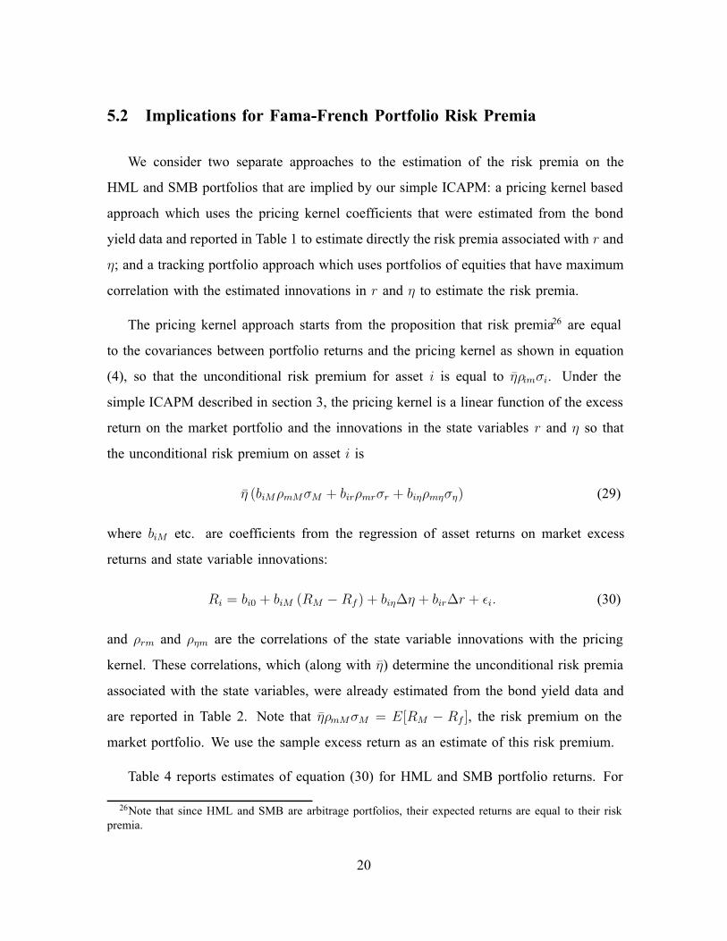
The primary data set consists of monthly observations of inflation and the yields on

eight synthetic constant maturity zero coupon U.S. treasury bonds with maturities of 3, 6

months, and 1, 2, 3, 4, 5, and 10 years for the period from January 1952 to December

2000. Table 1 reports summary statistics for the bond yield data. The sample mean

of the bond yields increases slightly with maturity, while the standard deviation remains

relatively constant across maturities. The inflation rate during the same sample period is

calculated from the CPI and has a sample mean of 4.1% and a sample standard deviation

of 1.1%. The returns on 25 size and book-to-market sorted value weighted portfolios, the

CRSP value weighted market portfolio and the nominal short interest rate for the same

period are used for cross-sectional pricing tests.15

The time series of the state variables r, π and η, and their dynamics, are estimated

by using the model of nominal bond yields, equation (14), in a Kalman filter, to extract

the time series of the unobservable state variables from data on bond yields and inflation.

Details of the estimation are presented in Appendix C. In summary, there are n observation

equations based on the yields at time t, yτj ,t, on bonds with maturities τj , j = 1, · · · , n.The observation equations are derived from equation (14) by the addition of measurement

errors, ετj :

yτj ,t ≡ − lnN(t, t+ τj)

τj= −A(t, τj)

τj+B(τj)

τjrt +

C(τj)

τjπt +

D(τ)

τηt + ετj (t). (23)

The measurement errors, ετj (t), are assumed to be serially and cross-sectionally un-

correlated, and to be uncorrelated with the innovations in the transition equations, and

their variance is assumed to be of the form: σ2(ετj ) = σ2b/τj where σb is a parameter to

15We thank Luis Viceira and Robert Bliss for providing the bond yield data. Our data start in January

1952 because the Federal-Treasury Accord that re-asserted the independence of the Fed from the Treasury

was adopted in March 1952. Equity market data are taken from the website of Ken French.

13

be estimated. The final observation equation uses the realized rate of inflation,Pt−Pt−∆t

Pt−∆t,

Pt − Pt−∆t

Pt−∆t

= π∆t+ εP (t). (24)

The transition equations are the discrete time versions of equations (5.2), (5.3) and

(12), the equations that describe the dynamics of the state variables, r, η, and π.

5 Empirical Results

In Section 5.1 we show that the time series of nominal bond yields and inflation

provide strong evidence of time variation in both the real interest rate and the Sharpe

ratio, that there are risk premia associated with these variables; that these variables are

associated with the market dividend yield and the equity premium; and that innovations in

the estimates of these state variables are correlated with the returns on the Fama-French

hedge portfolios. In Section 5.2, we consider the quantitative implications of the model

estimates for the risk premia on HML and SMB. Finally, in Section 5.3 we consider the

ability of portfolios formed to track innovations in r and η to explain the cross section of

returns on 25 size and book-to-market sorted equity portfolios.

5.1 State Variable Estimates

In this section we report Kalman filter estimates of the stochastic process for the state

variables, r, π, and η, as well as the estimated time series of the state variables. In order

to identify the process for the Sharpe ratio, η, it is necessary to impose a restriction that

determines the overall favorableness of investment opportunities.16 The restriction we

impose is that η = 0.7. This value was chosen after fitting an EGARCH model to the

market excess return and using the resulting times series of volatility estimates to calculate

16Equation (4) shows that the structure of risk premia is invariant up to a scalar multiplication of η and

the vector of inverse security correlations with the pricing kernel with typical element, 1/ρV m.

14

a time series of realized equity market Sharpe ratios. This series has a mean of 0.57.17

Since η is the maximum Sharpe ratio of the economy, we set η to 0.7 to allow for the

fact that the equity market portfolio is not mean-variance efficient. This normalization

affects only estimates of the scale of η and correlations of other variables with η. Finally,

to improve the efficiency of estimation, r and π were set equal to their sample means,

and σP , the volatility of unexpected inflation, was set equal to the CPI inflation sample

volatility of 1.12%. As a result of predetermining these parameter values, the standard

errors of all other parameters reported in Panel B of Table 1 are understated.

Since the bond yield data were constructed by estimating a cubic spline for the spot

yield curve from the prices of coupon bonds, the bond yields are measured with error.

The variance of the yield measurement error was assumed to be inversely proportional

to maturity τ . The estimate of the measurement error parameter, σb, implies that the

standard deviation of the measurement error varies from 30 basis points for the three

month maturity to 5 basis points for the ten year maturity, so that the model fits the yield

data quite well.

The volatility of expected inflation, σπ , is estimated to be around 1.06% per year,

while κπ is close to zero, so that the expected rate of inflation rate follows almost a

random walk.18 The estimated volatility of the real interest rate process, σr, is 2.34%

per year, so that the real interest rate is much more volatile than the expected inflation

rate.19 The estimated mean reversion intensity for the interest rate, κr, is 0.124 per year

which implies a half life of about 5 years. The volatility of the Sharpe ratio process, ση,

is 0.18 per year which compares with the imposed long run mean value of 0.70; the mean

reversion intensity for the Sharpe ratio is similar to that for the real interest rate.

17The excess return of the CRSP value weighted market portfolio during the sample period has a mean

of about 0.62% and a standard deviation of 4.23% per month, implying a Sharpe ratio of 0.5 if volatility is

assumed to be constant. Mackinlay (1995) reports an average Sharpe ratio of around 0.40 for the S&P500for the period 1981-1992.

18Campbell and Viceira (2001) also find that the expected rate of inflation is close to a random walk in

a similar setting, using a model with constant risk premia.19Campbell and Viceira’s(op. cit.) estimate is only 0.5% per year.

15

To place the volatility of the real interest rate and the Sharpe ratio in perspective,

suppose that the volatility of the market return, σM , is constant at 15%. Then if the

correlation between the market and the pricing kernel is, say, 0.9,20 the estimated volatility

of the expected market return that is due to the volatility of the Sharpe ratio is 0.15 ×0.18 × 0.9 = 2.43%, which is close to the estimated volatility attributable to the real

interest rate (2.34%), so that variation in r and in η are of comparable importance for the

variation in the expected return on the equity market. Note, however, that the correlation

between innovations in r and in η is −0.45, so that a significant part of the effect of

the innovations in these two variables on the expected market return is offsetting. The

Wald statistic for the null hypothesis that ση = κη = 0 (so that η is a constant) is

highly significant, providing strong evidence, given the pricing model, that the Sharpe

ratio is time varying. Finally, the t-statistics on ρηm and ρrm strongly reject the null that

the opportunity set state variables, r and η, are unpriced. However, this is not in itself

evidence in favor of the ICAPM, because it is possible that the risk premia are due to the

correlation of these variables with the market portfolio as in the classical CAPM; we shall

investigate this further below. The t-statistics on ρPm and ρπm are either not significant or

are only marginally significant: thus there does not appear to be a risk premium associated

with inflation.

Figures 1 and 2 plot the time series of the estimated real interest rate and Sharpe

ratio. The estimated real interest rate reaches a maximum of 7.58% in mid-1982, and a

minimum of -1.9% in the Fall of 1992: it is positive for most of the sample period and

its average value is 3.5%. The estimated Sharpe ratios also show considerable variation,

reaching a maximum of 1.37 in March 1985 and a minimum of -1.16 in March 1980.21

Recessions, which are represented by the shaded areas in the figures,22 are generally

20This value corresponds to the point estimate from equation 26below.21Boudoukh et. al.(1993) find evidence that the ex-ante equity market risk premium is negative in periods

in which Treasury Bill rates are high. In March 1980 the Treasury Bill rate was over 14%.22The period of recession is measured from peak to trough as determined by the National Bureau of

Economic Research.

16

associated with a declining real interest rate but an increasing Sharpe Ratio. Whitelaw

(1997) and Perez-Quiros and Timmermann (2000) have found similar cyclical patterns

in the Sharpe ratio in the equity market.23 The correlation between the estimated levels

of r and η is about −0.22 which is consistent with the negative correlation between the

innovations in these variables; high real interest rates appear to be associated with low

Sharpe ratios.

To assess the empirical relevance of the state variable estimates for the equity market,

we examine their relations with the realized Sharpe ratio of the CRSP value weighted

index, and with the dividend yields on the S & P 500 index. Note that equation (4)

implies that the equity market risk premium is related to η by:

µM − r = ηρMmσM

which implies that the equity market Sharpe ratio can be written as:

SHM ≡ µM − r

σM= ηρMm. (25)

The realized market Sharpe ratio for each month, SHRM , is constructed by dividing

the market excess return for that month by the EGARCH fitted volatility. Regressing

SHRM on η−1 yields the following results with the Newey-West adjusted t-ratios in the

parentheses:

SHRM = 0.15

(0.64)

+ 0.90η−1,

(2.24)

R2

0.01(26)

Thus, the Sharpe ratio that we have estimated using data on bond yields and inflation has

significant information for normalized excess returns on the stock market. The estimated

coefficient of η−1 implies that ρMm = 0.9,24 and the lack of significance of the intercept

23Fama and French (1989) have also documented common variation in expected returns on bonds and

stocks that is related to business conditions.24Note that the estimated correlation depends on the assumed value of η. Shanken (1987) presents

evidence that one can reject the hypothesis that the correlation between a linear combination of the CRSP

17

is consistent with the theoretical specification (25).

The valuation model (17) implies that there will be a relation between the dividend

yield of a security and the state variables. Thus, defining xt ≡ Xt/Pt as the real dividend,

equation (17) of Theorem 3 implies that the price-dividend ratio of the security is given

by:

Vtxt

=

∫ ∞

t

exp[A(s− t)− B(s− t)r − C(s− t)π − D(s− t)η + F (s− t)g]ds

where B(s−t) > 0, C(s−t) > 0, F (s−t) > 0 for all parameter values, and D(s−t) > 0

given that our parameter estimate satisfies ρmr < 0. The log of the dividend yield, y, is

related to the state variables by the approximate relation:

y ≡ ln

(xtVt

)≈ b0 + b1rt + b2πt + b3ηt + b4gt, (27)

and the valuation model implies the following coefficient restrictions:

b1, b2, b3 > 0, b4 < 0. (28)

To test these restrictions, equation (27) was estimated using the S&P500 dividend yield

as reported by DRI and the consensus forecast long run earnings growth rate25 for the S

& P 500. The availability of the growth rate forecast data restricts the sample period to

the period from January 1985 to December 2000.

During this sample period, the estimated values of r, π, η, g and y all have first order

autocorrelation of 0.95 or higher. Panel A of Table 2 reports the results of unit root tests

for r, π, η, g and y. The Augmented Dickey Fuller test cannot reject the null of a unit

root for r, π, g and y, but does reject for η at 5% significance. The Phillip-Perron test,

however, cannot reject the unit root null for any of the series. The Johansen cointegration

test rejects the null of no-cointegration at the 1% significance level whether or not π is

equal weighted index and a bond portfolio and the pricing kernel exceeds 0.7. Kandel and Stambaugh

(1987) report similar evidence for the value weighted index.25We thank Thomson Financial for providing these data.

18

included. The normalized cointegrating coefficients are reported in Panels B and C of

Table 2. When π is included, the cointegrating coefficients for π, η and g are highly

significant, but the coefficient for r is not. When π is not included, the coefficients for r,

η and g are all significant. Note that the coefficients b0, · · · , b4 which have the opposite

sign to the cointegrating coefficients and are otherwise identical, are consistent with the

model prediction. Thus the state variables r, (π), and η are significantly related to the

level of equity prices as measured by the market dividend yield.

If the ICAPM is to provide an explanation for the risk premia on the FF hedge

portfolios that are not explained by their covariance with the market return, innovations in

the investment opportunity set state variables must be correlated with the returns on these

portfolios, after allowing for the effect of the market return. To test this, we calculate

the innovations, εr, επ and εη , in the state variable estimates using the parameter values

reported in Table 2, and then regress these estimated innovations on the returns on the

three FF portfolios. The results are reported in Panel A of Table 3. The innovation in r

is significantly related to both the excess return on the market portfolio and to the return

on the HML portfolio. The innovation in η is significantly related to the returns on both

the SMB and HML portfolios. The innovation in π is not significantly related to any

of the portfolio returns.

Panel B of Table 3 reports the results of regressing the market, SMB and HML

portfolio returns on the innovations in the state variables. It provides further support that

SMB returns are significantly related to all three state variable innovations while HML

returns are significantly related to the innovations to η.

The significant values of ρrm (−0.85) and ρηm (0.73) reported in Table 1 imply that

there are indeed risk premia associated with innovations in r and η. In the next section,

we consider whether the estimated risk premia associated with these innovations, together

with the estimated loadings of the SMB and HML portfolio returns on the innovations,

are sufficient to account for the observed returns on these portfolios.

19

5.2 Implications for Fama-French Portfolio Risk Premia

We consider two separate approaches to the estimation of the risk premia on the

HML and SMB portfolios that are implied by our simple ICAPM: a pricing kernel based

approach which uses the pricing kernel coefficients that were estimated from the bond

yield data and reported in Table 1 to estimate directly the risk premia associated with r and

η; and a tracking portfolio approach which uses portfolios of equities that have maximum

correlation with the estimated innovations in r and η to estimate the risk premia.

The pricing kernel approach starts from the proposition that risk premia26 are equal

to the covariances between portfolio returns and the pricing kernel as shown in equation

(4), so that the unconditional risk premium for asset i is equal to ηρimσi. Under the

simple ICAPM described in section 3, the pricing kernel is a linear function of the excess

return on the market portfolio and the innovations in the state variables r and η so that

the unconditional risk premium on asset i is

η (biMρmMσM + birρmrσr + biηρmηση) (29)

where biM etc. are coefficients from the regression of asset returns on market excess

returns and state variable innovations:

Ri = bi0 + biM (RM − Rf ) + biη∆η + bir∆r + εi. (30)

and ρrm and ρηm are the correlations of the state variable innovations with the pricing

kernel. These correlations, which (along with η) determine the unconditional risk premia

associated with the state variables, were already estimated from the bond yield data and

are reported in Table 2. Note that ηρmMσM = E[RM − Rf ], the risk premium on the

market portfolio. We use the sample excess return as an estimate of this risk premium.

Table 4 reports estimates of equation (30) for HML and SMB portfolio returns. For

26Note that since HML and SMB are arbitrage portfolios, their expected returns are equal to their risk

premia.

20

comparison, simple regressions of the portfolio returns on market returns are also reported.

The coefficient on ∆η is positive and significant for both HML and SMB. The coefficient

on ∆r is negative and significant for HML but positive and insignificant for SMB. The

significant coefficients of the SMB and HML portfolio returns on the innovations in r

and η after allowing for the effect of the market return imply that, if these state variables

are priced, then the risk premia on SMB and HML will differ from the predictions of the

simple CAPM, as previous authors have found.

Lines (1) and (4) of Table 4 report simple CAPM regressions for SMB and HML

for the whole sample period. The intercept for HML is 0.5% per month and is highly

significant: this is the familiar result that the relative returns on value and growth firms

cannot be explained by the CAPM. The intercept for SMB is −0.6% per month, so that

during this period large firms outperformed small firms; however, the intercept is not

significantly different from zero either for the whole sample period or for the two sub-

sample periods, and we conclude that there is no evidence of a size effect relative to the

CAPM. It is nevertheless possible that there will be a size effect relative to the ICAPM.

The unconditional risk premium associated with r (η) is ηρmrσr (ηρmηση). The

parameter estimates from Table 1 imply that the risk premia associated with r, η, and π

are, respectively, -1.39%, 9.25% and 0.15% per annum, while the market risk premium

for this period was 7.40%. However, the estimates of biη or bir shown in Table 4 are so

small that the resulting estimates of the risk premia of HML and SMB that are associated

with the two state variables are trivial: for HML (SMB) the annualized risk premium

associated with r is only 0.64% (−0.31%), and associated with η is 0.31% (0.37%). Thus,

the pricing kernel that was estimated from the bond yield data, together with the estimated

portfolio sensitivities to the innovations in r and η reported in Table 4, cannot account

for the high return on HML.

A possible reason for the failure of the pricing kernel approach is that ∆r and ∆η, the

innovations in the state variables, are measured with error. This could bias the resulting

21

estimates of biη and bir and affect our conclusions about the ability of the estimated

pricing kernel to capture the risk premia on HML and SMB. The “tracking portfolio”

approach of Breeden (1979), Breeden, Gibbons, and Litzenberger (1989) and Lamont

(2001) uses instrumental variables to avoid the errors-in-variables problems associated

with the pricing kernel approach. Lamont (2001) succinctly summarizes the properties of

tracking portfolios: “A tracking portfolio for any variable y can be obtained as the fitted

value of a regression of y on a set of base asset returns. The portfolio weights for the

economic tracking portfolio for y are identical to the coefficients of an OLS regression.

If y happens to be a state variable for asset pricing, then a multi-factor model holds with

one of the factors being y's tracking portfolio (Breeden, 1979).”

Following the above authors, we first construct “tracking” portfolios which have max-

imal correlations with the estimated innovations in r, and η, and then use the returns on

these portfolios as instruments for ∆r, ∆π and ∆η in a factor portfolio regression. The

tracking portfolios are constructed by regressing the estimated innovations in the state

variables on the excess returns on the six size and value sorted portfolios of Fama and

French (the base assets) and including ηt−1 as a control for the expected excess returns

on the base assets.27 Since η is measured with error, tracking portfolios were constructed

both with and without η as a control.

It follows from the properties of tracking portfolios that, under the null hypothesis

of the simple ICAPM, asset risk premia, Ri, are related to the expected returns on the

tracking portfolios by:

E [Ri] = b∗iME [RM − Rf ] + b∗iηE [Rη] + b∗irE [Rr] , (31)

where Rη and Rr are the returns on the tracking portfolios for r and η, and b∗iM etc. are

27We do not use bond portfolios as base assets because the estimates of r and η are linear functions of

bond yields. As a result, tracking portfolios that included bond portfolios as base assets would be dominated

by the bond portfolio returns and their returns would be subject to the same errors as the original estimates

of the state variable innovations.

22

the coefficients from the regressions of asset i returns on the market and tracking portfolio

returns.

Regressions to determine the composition of the tracking portfolios are reported in

Table 5 Panel A. For both ∆r and ∆η, the coefficients of the base assets are jointly

significant at better than the 1% level, and the inclusion of η as a control variable has

little effect on the coefficients. Since the control variable ηt−1 enters insignificantly in all

the regressions, the tracking portfolios were constructed using the coefficients reported in

columns (1) and (3). Panel B of Table 5 reports the correlations between the returns on

the tracking portfolios, Rr and Rη and the returns on HML and SMB. HML is positively

correlated with Rη and negatively correlated with Rr, both correlations being around

0.40 in absolute value. SMB has a correlation of 0.59 with Rη, and only 0.16 with Rr.

Multiple regressions of HML and SMB on the two mimicking portfolio returns yield R2’s

of 0.26 (HML) and 0.50 (SMB). Thus the mimicking portfolios, despite being formed

from size and book-to-market sorted portfolios like the FF portfolios, are not just linear

combinations of the FF portfolios.

Condition (31) implies that, under the null hypothesis, the intercept from the regression

of the excess returns of any asset on the excess returns on the market portfolio and the

returns on the tracking portfolios will be equal to zero. Panel A of Table 6 reports

the results of such regressions for the HML and SMB portfolios for the period January

1952 to December 2000. In striking contrast to the large and significant intercept for the

CAPM regression for HML reported in Table 4, the intercepts for both HML and SMB

are now both very close to zero and statistically insignificant: 0.0% per month for HML

and −0.15% per month for SMB. These regressions imply that the returns on both HML

and SMB are consistent with the simple ICAPM when the tracking portfolio approach is

used to avoid the errors-in-variables problem. Panels B and C in Table 6 show that the

results are robust across the two halves of the sample period. The least favorable results

are during the first half of the sample period when the intercepts are at the margin of

significance for both HML and SMB if tracking portfolios are formed separately for each

23

sub period; they are not significant when the tracking portfolios are formed using data

from the whole sample period. Thus, it seems that, over this sample period, the return

on the HML portfolio is not anomalous when viewed through the lens of this simple

ICAPM. The returns on SMB are consistent with both the simple CAPM (Table 4, line 3)

and the ICAPM (Table 4 Panel B). Thus, there appears to be no need to invoke investor

irrationality,28 or statistical biases,29 in order to explain the returns on these portfolios.

Table 7 analyzes the contribution of each tracking portfolio to the explanation of the

HML and SMB portfolio returns. Panel A reports the means and standard deviations of

the three portfolio excess returns. The implied sample Sharpe ratios for the market, r, and

η tracking portfolios are 0.51, -0.86 and 0.85 respectively. The estimated unconditional

Sharpe ratios associated with r and η risk implied by the pricing kernel estimates in Table

130 are -0.59 and 0.51. It is encouraging that the signs of the pricing kernel estimates of the

risk premia are the same as those of the tracking portfolio estimates and of comparable

magnitude. The pricing kernel estimates of the Sharpe ratios are proportional to the

unconditional value of the overall Sharpe ratio, η, which we have assumed to be 0.7. This

value is obviously low relative to the sample Sharpe ratios for the tracking portfolios. It

is interesting to note that the sample Sharpe ratios of the tracking portfolios are large

relative to those of HML and SMB, which are 0.47 and 0.12 respectively.

The estimated coefficients of the regression of returns on the market and tracking

portfolio returns reported in Table 5B, together with the sample means of the tracking

portfolio returns reported in Table 7A, were used to calculate conditional estimates of the

risk premia given by equation (31).31 These are reported in Panel B of Table 6. For the

HML portfolio, the estimated risk premium per year for market risk is -3.39%, for r risk

is 5.38%, and for η risk is 2.41%; the sum of these risk premia (4.40%) is almost identical

to the sample mean excess return on HML (4.40%). For the SMB portfolio, the estimated

28See, e.g., Lakonishok, Shleifer and Vishny (1994).29Kothari, Shanken and Sloan (1995) and Mackinlay (1995)30The unconditional Sharpe ratio associated with r risk is ηρmr and similarly for η.31The risk premium estimates are conditional on the sample mean returns of the tracking portfolios.

24

risk premia for market, r, and η risk are 2.13%, -5.39%, and 6.32%, respectively: the

total risk premium predicted by the regression is 3.1%, which is twice as high as the 1.2%

sample mean excess return but is not significantly different from it. Line (4) of Table 4

shows that the SMB risk premium is also consistent with the CAPM since the estimated

intercept is not significantly different from zero. In summary, exposure to r risk earns the

HML portfolio an estimated premium of 5.38% while it earns SMB a premium of -5.39%.

Exposure to η risk earns HML a premium of 2.41% and SMB a premium of 6.32%. As

we conjectured, high and low book-to-market, and small and big, firms have different

exposures to innovations in r and η. The realized returns on both HML and SMB are

consistent with a simple ICAPM in which the state variables are the real interest rate, r,

and the Sharpe ratio η.

A criticism that is sometimes made of the tracking portfolio approach is that it uses

returns on a set of factor portfolios to explain the returns on other portfolios so that it is

not surprising to have high R2 and highly significant regression coefficients as reported

in Table 5B. While this is true, the test of the equilibrium model is not the R2 or the

signifiance of the slope coefficients, but the significance of the regression intercept, and

nothing in the tracking portfolio approach per se guarantees that this will be insignificant.

For example, if the signs of the returns on the tracking portfolios were reversed, the

regression intercepts in Table 5B would be significant and the ICAPM would be rejected.

And, as we shall see in the following section, the tracking portfolio approach is not

entirely successful in explaining the returns on a broader set of assets.

5.3 Cross-sectional Pricing

In order to test whether the simple ICAPM can explain the returns on a broader set of

portfolios, the excess returns on 25 FF size and book-to-market portfolios were regressed

on the market excess returns and the returns on the r and η mimicking portfolios for the

25

period January 1952 - December 2000.

Ri −Rf = αi + βi,Mkt [RM − Rf ] + βi,ηRη + βi,rRr (32)

and the null hypothesis is αi = 0, ∀i = 1, · · · , 25. For comparison, the regressions were

repeated using the Fama-French HML and SMB portfolios in place of the mimicking

portfolios. The results are reported in Tables 8 and 9 which include results for the two

halves of the sample period.

Small firms tend to load positively on both Rr and Rη, and large firms negatively.

High book-to-market portfolios tend to have higher loadings on Rη than low book-to-

market firms, and lower loadings on Rr and the pattern is stable across the sub-periods.

In the tracking portfolio regressions, the estimates of α are insignificant for 20 out of the

25 portfolios, but the Gibbons, Ross, and Shanken (1989) (GRS) test of the hypothesis

that α’s of the 25 portfolios are jointly zero yields a test statistic of F (25, 560) = 2.09

which is significant at the 1% level. When the regression is repeated using the Fama-

French factors, SMB and HML, in place of the tracking portfolios, the α estimates are

significant for 8 out of the 25 portfolios, and the GRS F-statistic is 2.78, also rejecting

the hypothesis. The tests are repeated for two and four equal sub-periods. The F-test

has values of 2.04 and 2.46 for the two sub-period tracking portfolio regressions, and

has values of 2.08 and 3.22 for the corresponding FF regressions. The null hypothesis is

rejected at the 1% significance for all the sub-periods. When the sample is divided into

four equal sub periods, the F-statistics for the tracking portfolio regressions are 1.52, 1.24,

1.04 and 2.93, with p-values of 0.07, 0.22, 0.42 and less than 0.01: the null is rejected

only in the last sub-period, from October 1988 to December 2000. The corresponding

F-statistics for the FF regressions are 2.22, 1.11, 1.33 and 3.35, with p-values of less than

0.01, 0.34, 0.16 and less than 0.01, rejecting the null in the first and last sub-periods.

The individual test results are only reported for two equal sub-periods. In summary, the

tests reject both the FF 3-factor model and the simple ICAPM for this sample period.

26

However, an implicit assumption in the above tests is that the Treasury Bill rate is

the appropriate measure of the riskless interest rate, and there is now evidence that the

Treasury Bill rate is unduly low relative to other short term rates,and it is certainly below

the rate at which investors can borrow.32 We therefore re-estimate equation (32) by non-

linear least squares, allowing the riskless interest rate to exceed the Treasury Bill rate

by a constant, λ. The estimate of λ in the tracking portfolio regressions is 0.12% per

month, or 1.44% per year with a t-statistic of 2.01. The corresponding figures for the FF

regressions are 1.69% per month, or an annualized figure of over 20% with a t-statistic of

5.58: this value of λ clearly makes the estimated reward for market risk negative in the

FF regressions. However, likelihood ratio tests of the hypothesis that the α’s of the 25

portfolios are jointly equal to zero in this expanded model yield test statistics of χ2(24)

equal to 49.40 and 46.96 for the tracking portfolio and FF regressions respectively: again,

the null hypothesis of the asset pricing model is rejected at better than the 1% level in

both cases.33

Inspection of the α’s in Tables 7 and 8, and of the mean portfolio residuals in the

regressions in which λ is allowed to be non-zero, reveals that it is the lowest book-to-

market portfolios whose returns deviate most strongly from the model predictions. When

the tracking portfolio regressions are re-estimated excluding the five portfolios with the

lowest B/M ratios, the estimate of λ becomes insignificant (0.13% per month with t-

statistic of 1.44), and the likelihood ratio statistic is χ2(19) = 27.2 which is not significant.

Thus the simple ICAPM is able to price all but the lowest B/M quintile of portfolios.

Similar results are obtained when the FF regressions are repeated excluding the lowest

B/M quintile: the likelihood ratio statistic is χ2(19) = 28.6 which is not significant.34

32Longstaff (2000, p400) argues that “the institutional demand for Treasury Bills with their regulatory,

tax, credit, and liquidity characteristics makes Treasury Bills generically special” which depresses their

yields. See Brennan (1971) for a simple asset pricing model with different borrowing and lending rates.33See Judge et al. (1982) for the log likelihood ratio test. Shanken (1986) argues that inferences obtained

by treating λ as if it were the true parameter values are biased toward acceptance of the null hypothesis

(p-value too high). Since the p-values associated with the reported χ2 statistics is an upper bound, the

rejection of null could be stronger than reported here.34Note that the p-value associated with the χ2(19) test statistics is only an upper bound. The true p-value

27

However, the estimate of λ is still an unreasonable 1.45% per month with a t-statistic of

4.56.

When the 20 portfolio regressions are repeated imposing the constraint λ = 0 and

using tracking portfolios, the GRS test yields a test statistic of F (20, 564) = 1.45 with

a p-value of 0.09, failing to reject the null hypothesis that the α’s of these 20 portfolios

are jointly zero. When the regressions are repeated using the Fama-French factors, SMB

and HML, in place of the tracking portfolios, the GRS F-statistic is 2.08, rejecting the

hypothesis at the 1% level. Thus, when attention is restricted to the 20 portfolios that

exclude the lowest B/M quintile, the simple ICAPM with λ = 0 cannot be rejected, while

the FF 3-factor model is easily rejected.

In summary, both the simple ICAPM and the FF three-factor model are rejected when

the assets to be priced are 25 size and book-to-market sorted portfolios for the period

1952-2000, even when the margin of the riskless rate over the Treasury Bill rate is left

as a free parameter. Both models are able to price the remaining 20 portfolios when the

5 portfolios with the highest book-to-market ratios are excluded and the riskless rate is

allowed to differ from the Treasury Bill rate. However, in this setting, the FF model

implies that the effective riskless interest rate is over 17% above the Treasury Bill rate

which makes the implied reward to market risk negative. When the constraint that the

riskless rate be equal to the Treasury Bill rate is imposed, the simple ICAPM is not

rejected on the 20 portfolio data while the FF three-factor model is.

Lo and MacKinlay (1990) advise caution in drawing inferences from samples of

characteristic sorted data such as the size and book-to-market sorted portfolios. Therefore,

as a robustness check we repeat the analysis using the returns on 30 industrial portfolios

based on 4-digit SIC codes.35 In order to ensure that the errors in the tracking portfolio

returns are orthogonal to the returns to be explained, the tracking portfolios are re-formed

may reject the null.35The data are taken from Ken French’s website which contains the definitions of the 30 industries.

28

by regressing the estimated innovations in r and η on the returns on the 30 industrial

portfolios. Then the returns on the 30 industrial portfolios are regressed first on the market

excess return (CAPM); secondly, on the market excess return and the returns on HML

and SMB (Fama-French 3-factor model); and finally on the market excess return and the

tracking portfolio returns, Rr and Rη, (ICAPM). Under the null hypothesis corresponding

to each of these models the intercepts from these regressions, α, are equal to zero. The

estimated intercepts and their associated t-ratios are reported in Table 10. The largest

intercept is for ‘Smoke’ and is of the order of 5.5-6.5% per year for the three models.

The estimated intercepts for ‘Health’ and ‘Food’ are also large for all three models, of

the order of 2.3-5.6% per year for the three models. The ICAPM performs the best of the

three models in the sense that the average absolute mispricing across the 30 portfolios is

only 1.5% per year, as compared with 1.8% for the CAPM, and 2.6% for the FF model.

The GRS F−statistics which are reported in Table 10 reject the null hypothesis that the

intercepts are jointly zero across the 30 portfolios for both the CAPM and the FF model.

However, the null is not rejected for the ICAPM. The failure to reject when the (industry)

portfolios are not formed on the basis of a characteristic which is known to be associated

with returns is consistent with Lo and Mackinlay’s warning that the characteristic based

portfolio data are likely to reject too often.

6 Conclusion

In this paper we have developed, estimated, and tested a simple model of asset valua-

tion for a setting in which real interest rates and risk premia vary stochastically. The model

implies that zero-coupon nominal bond yields are linearly related to the state variables

r and η, the real interest rate and the maximal Sharpe ratio, as well as to the expected

rate of inflation, π. Data on bond yields and inflation are used to provide estimates of

the state variables and of the parameters of their joint stochastic process. The estimated

real interest rate and Sharpe ratio both show strong business cycle related variation, the

29

Sharpe ratio rising, and the real interest rate falling, during recessions. The Sharpe ratio

estimate is shown to be related to the excess return on the equity market portfolio, and the

level of stock prices as measured by the market dividend yield is shown to be related to

both the Sharpe ratio and real interest rate estimates. All of these findings are consistent

with the model predictions.

When portfolios of 6 size and book-to-market sorted portfolios are formed to track

the innovations in the state variables, it is found that, as conjectured, the risk premia on

the Fama-French HML and SMB portfolios over the period 1952-2000 are explained by

an ICAPM in which the tracking portfolios are used to represent the innovations in the

state variables. When the tracking portfolios are used to price 25 size and book-to-market

sorted portfolios the ICAPM is rejected even when the riskless interest rate is allowed

to differ from the Treasury Bill rate by a constant. However, the Fama-French 3-factor

model fares no better in explaining these portfolio returns. When the 5 portfolios with

the lowest book-to-market ratios are excluded from the analysis the results change. Now,

neither the ICAPM nor the FF 3-factor model can be rejected. But while the estimated

excess of the risk free rate over the Treasury Bill rate is insignificant for the ICAPM, it

is over 17% per year and highly significant for the FF model: this makes the estimated

reward for bearing market risk negative. The FF 3-factor model, but not the ICAPM, is

rejected on the 20 portfolio data when the risk free rate is assumed to be equal to the

Treasury Bill rate.

Lo and Mackinlay (1990) have warned that, when asset pricing models are tested on

the returns of portfolios that have been formed on the basis of some characteristic which

is known to be associated with returns, the models are likely to be rejected too often.

Since the size and book-to-market portfolios seem to meet this criterion, we also test the

model using the returns on 30 industry portfolios. The model is not rejected using these

returns, although both the simple CAPM and the Fama-French model are rejected. These

results with a highly simplified ICAPM are sufficiently encouraging to warrant further

empirical investigation of the ICAPM. We stress the need in empirical implementation of

30

the ICAPM to pay careful attention to the selection of state variables: the ICAPM is not

just another “factor model”; the state variables of the model must be limited to those that

predict future investment opportunities.

31

Appendix

A. Proof of Theorems 1 and 2

The real part of the economy is described by the processes for the real pricing kernel,

the real interest rate, and the maximum Sharpe ratio (5.1)-(5.3), while the nominal part of

the economy is described by the processes for the price level and the expected inflation

rate (11)-(12). Under the risk neutral probability measure Q, we can write these processes

as:

dr = κr(r − r)dt− σrρmrηdt+ σrdzQr (A1)

dπ = κπ(π − π)dt− σπρmπηdt+ σπdzQπ (A2)

dη = κ∗η(η

∗ − η)dt+ σηdzQη (A3)

where κ∗η = κη + σηρmη and η∗ = κη ηκ∗η

.

Let y, whose stochastic process is given by (6), denote the expectation of a nominal

cash flow at a future date T , XT . The process for ξ ≡ y/P , the deflated expectation of

the nominal cash flow, under the risk neutral probability measure can be written as:

dξ

ξ=

[−π − σyσPρyP + σ2P − η(σyρym − σP ρPm)

]dt+ σydz

Qy − σPdz

QP . (A4)

The real value at time t of the claim to the nominal cash flow at time T , XT , is given by

expected discounted value of the real cash flow under Q:

V (ξ, r, π, η, T − t) = EQt

[XT

PTexp− ∫ T

t r(s)ds

]= EQt

[yTPT

exp− ∫ Tt r(s)ds

]= EQt

[ξT exp

− ∫ Ttr(s)ds

](A5)

32

Using equation (A4), we have

ξT = ξt exp

(−1

2σ2y +

1

2σ2P

)(T − t)− (σyρym − σPρPm)

∫ T

t

η(s)ds

−∫ T

t

π(s)ds+ σy

∫ T

t

dzQy − σP

∫ T

t

dzQP

. (A6)

A tedious calculation from equations (A1), (A2), and (A3) gives us the following

results: ∫ T

t

η(s)ds = ηt1− e−κ

∗η(T−t)

κ∗η

+ η∗[T − t− 1− e−κ

∗η(T−t)

κ∗η

]

+ ση

∫ T

t

1− e−κ∗η(T−s)

κ∗η

dzQη (s), (A7)

∫ T

t

π(s)ds = πt1− e−κπ(T−t)

κπ+

(π − σπρmπ η

∗

κπ

) [T − t− 1− e−κπ(T−t)

κπ

]

+

(σπρmπηtκ∗η − κπ

− σπρmπ η∗

κ∗η − κπ

) [1− e−κ

∗η(T−t)

κ∗η

− 1− e−κπ(T−t)

κπ

]

+σπρmπσηκ∗η − κπ

∫ T

t

[1− e−κ

∗η(T−s)

κ∗η

− 1− e−κπ(T−s)

κπ

]dzQη (s)

+ σπ

∫ T

t

1− e−κπ(T−s)

κπdzQπ (s) (A8)

and ∫ T

t

r(s)ds = rt1− e−κr(T−t)

κr+

(r − σrρmrη

∗

κr

) [T − t− 1− e−κr(T−t)

κr

]

+

(σrρmrηtκ∗η − κr

− σrρmrη∗

κ∗η − κr

) [1− e−κ

∗η(T−t)

κ∗η

− 1− e−κr(T−t)

κr

]

+σrρmrσηκ∗η − κr

∫ T

t

[1− e−κ

∗η(T−s)

κ∗η

− 1− e−κr(T−s)

κr

]dzQη (s)

+ σr

∫ T

t

1− e−κr(T−s)

κrdzQr (s) (A9)

33

Substituting equations (A6)-(A9) into equation (A5) yields

V (ξ, r, π, η, T − t) = ξtGEQt[expψ

], (A10)

where G is given by

G = exp E(τ)− B(τ)rt − C(τ)πt −D(τ)ηt (A11)

and

B(τ) =1− e−κr(T−t)

κr(A12)

C(τ) =1− e−κπ(T−t)

κπ(A13)

D(τ) = d1 + d2e−κ∗ητ + d3e

−κrτ + d4e−κπτ (A14)

E(τ) =

(−1

2σ2y +

1

2σ2P − r − π − d1κ

∗ηη

∗)τ +

(r − d3κ

∗ηη

∗)B(τ)

+(π − d4κ

∗η η

∗)C(τ)− d2κ∗ηη

∗d(τ) (A15)

with d(τ) =(1− e−κ

∗η(T−t)) /κ∗

η, and finally

d1 = −σPρmP − σyρmyκ∗η

− σrρmrκr κ∗

η

− σπρmπκπκ∗

η

(A16)

d2 = −σyρmyκ∗η

− σrρmr(κ∗

η − κr)κ∗η

− σπρmπ(κ∗

η − κπ)κ∗η

(A17)

= −d1 − d3 − d4

d3 =σrρmr

(κ∗η − κr)κr

(A18)

d4 =σπρmπ

(κ∗η − κπ)κπ

(A19)

The stochastic variable ψ is a linear function of the Brownian motions:

ψ = ση

∫ T

t

[d2

(1− e−κ

∗η(T−s)) + d3

(1− e−κr(T−s)) + d4

(1− e−κπ(T−s))] dz∗η(s)

− σrκr

∫ T

t

(1− e−κr(T−s)) dz∗r (s)− σπ

κπ

∫ T

t

(1− e−κπ(T−s)) dz∗π(s)

+ σy

∫ T

t

dz∗y(s)− σP

∫ T

t

dz∗P (s). (A20)

34

Since ψ is normally distributed with mean zero, V is given by

V (ξ, r, π, η, T − t) = ξtG1 exp

1

2Vart(ψ)

(A21)

Calculating Vart(ψ) and collecting terms, we get that

V (ξ, r, π, η, T − t) = ξt exp A(τ)−B(τ)rt − C(τ)πt −D(τ)ηt (A22)

where

A(τ) = a1τ + a21− e−κrτ

κr+ a3

1− e−κπτ

κπ+ a4

1− e−κ∗ητ

κ∗η

+a51− e−2κrτ

2κr+ a6

1− e−2κπτ

2κπ+ a7

1− e−2κ∗ητ

2κ∗η

+a81− e−(κ∗η+κr)τ

κ∗η + κr

+ a91− e−(κ∗η+κπ)τ

κ∗η + κπ

+ a101− e−(κr+κπ)τ

κr + κπ. (A23)

Define a0 ≡ σrη

κr+ σπη

κπ+ σPη − σyη − κ∗

ηη∗, r∗ ≡ r− σPr−σyr

κr, and π∗ ≡ π− σPπ−σyπ

κπ,

35

then a1, . . . , a10 are expressed as

a1 = σ2P − σyP +

σ2r

2κ2r

+σ2π

2κ2π

+σrπκrκπ

+σ2η

2d2

1 − r∗ − π∗ + a0d1 (A24)

a2 = r∗ − σ2r

κ2r

− σrπκrκπ

− σrηκr

d1 + a0d3 + σ2ηd1d3 (A25)

a3 = π∗ − σ2π

κ2π

− σrπκrκπ

− σπηκπ

d1 + a0d4 + σ2ηd1d4 (A26)

a4 = a0d2 + σ2ηd1d2 (A27)

a5 =σ2r

2κ2r

+σ2η

2d2

3 −σrηκr

d3 (A28)

a6 =σ2π

2κ2π

+σ2η

2d2

4 −σπηκπ

d4 (A29)

a7 =σ2η

2d2

2 (A30)

a8 = −σrηκr

d2 + σ2ηd2d3 (A31)

a9 = −σπηκπ

d2 + σ2ηd2d4 (A32)

a10 =σrπκrκπ

− σπηκπ

d3 − σrηκr

d4 + σ2ηd3d4 (A33)

Theorems 1 and 2 follow as special cases of equation (A22). Theorem 1 is obtained

by setting σP and the parameters in the expected inflation process (A2) to zero. Theorem

2 is obtained by setting σy to zero.

Theorem 3 is more complicated because of the additional state variable g. Using the

same approach as above, we can derive that an equity value at time t is given by

V (X, r, π, η, g) = EQ[∫ ∞

t

Xs

Pse−

∫ str(u)duds

]=

Xt

Pt

∫ ∞

t

v(s− t, r, π, η, g)ds (A34)

where Q denotes the risk neutral probability measure, and

v(s, r, π, η, g) = exp[A(s− t)−B(s− t)r − C(s− t)π − D(s− t)η + F (s− t)g]

36

where

B(s− t) = κ−1r

(1− e−κr(s−t)) (A35)

C(s− t) = κ−1π

(1− e−κπ(s−t)) (A36)

F (s− t) = κ−1g

(1− e−κg(s−t)) (A37)

D((s− t)) = d1 + d2e−κ∗η(s−t) + d3e

−κr(s−t) + d4e−κπ(s−t) + d5e

−κg(s−t) (A38)

A((s− t)) = a1(s− t) + a21− e−κr(s−t)

κr+ a3

1− e−κπ(s−t)

κπ+ a4

1− e−κ∗η(s−t)

κ∗η

+a51− e−2κr(s−t)

2κr+ a6

1− e−2κπ(s−t)

2κπ+ a7

1− e−2κ∗η(s−t)

2κ∗η

+a81− e−(κ∗η+κr)(s−t)

κ∗η + κr

+ a91− e−(κ∗η+κπ)(s−t)

κ∗η + κπ

+ a101− e−(κr+κπ)(s−t)

κr + κπ

+a111− e−(κ∗η+κg)(s−t)

κ∗η + κg

+ a121− e−(κg+κπ)(s−t)

κg + κπ+ a13

1− e−(κr+κg)(s−t)

κr + κg

+a141− e−κg(s−t)

κg+ a15

1− e−2κg(s−t)

2κg(A39)

κ∗η ≡ κη + σηρmη , and d1, . . . , d5, a1, . . . , a15 are constants whose values are available

upon request.

B. Expected Return

Applying Ito’s lemma to the V function from Theorem 1, the expected return on the claim

can be written as:

µ ≡ µ(r, η, τ) = −Aτ + rBτ + ηDτ +1

2D2σ2

η +BDρηrσησr +1

2B2σ2

r

−Dρyησyση − Bρyrσyσr −Dκη(η − η)− Bκr(r − r)

= Dτη +Bτr +Dκηη + Bκrr

= r + (Dτ +Dκη)η, (B1)

37

C. Details of Kalman Filter

The yield-based estimates of the state variable dynamics are derived by applying a

Kalman filter to data on bond yields and inflation using equations (23) and (24). The

transition equations for the state variables, r, π and η are derived by discretizing equations

(5.2), (5.3), and (12):

rt

πt

ηt

=

e−κr∆t 0 0

0 e−κπ∆t 0

0 0 e−κη∆t

rt−∆t

πt−∆t

ηt−∆t

+

r[1− e−κr∆t

]π

[1− e−κπ∆t

]η

[1− e−κη∆t

]

+

εr(t)

επ(t)

εη(t)

,(C1)

where the vector of innovations is related to the standard Brownian motions, dzr, dzπ and

dzη, by

εr(t)

επ(t)

εη(t)

=

σre−κrt

∫ t

t−∆teκrτdzr(τ)

σπe−κπt

∫ t

t−∆teκπτdzπ(τ)

σηe−κηt

∫ t

t−∆teκητdzη(τ)

, (C2)

and the variance-covariance matrix of the innovations is

Q =

σ2r

2κr

[1− e−2κr∆t

]σrσπρrπ

κr+κπ

[1− e−(κr+κπ)∆t

] σrσηρrη

κr+κη

[1− e−(κr+κη)∆t

]σrσπρrπ

κr+κπ

[1− e−(κr+κπ)∆t

] σ2π

2κπ

[1− e−2κπ∆t

] σπσηρπη

κπ+κη

[1− e−(κπ+κη)∆t

]σrσηρrη

κr+κη

[1− e−(κr+κη)∆t

] σπσηρπη

κπ+κη

[1− e−(κπ+κη)∆t

] σ2η

2κη

[1− e−2κη∆t

]

.

(C3)

The first n observation equations assume that the observed yields at time t, yτj ,t, on

bonds with maturities τj , j = 1, · · · , n, are given by equation (23) plus a measurement

error terms, ετj :

yτj ,t ≡ − lnV (t, t+ τj)

τj= −A(t, τj)

τj+B(τj)

τjrt +

C(τj)

τjπt +

D(τj)

τjη + ετj (t). (C4)

The measurement errors, ετj (t), are assumed to be serially and cross-sectionally uncorre-

lated and are uncorrelated with the innovations in the transition equations.

38

The n+ 1 observation equation uses the realized rate of inflation:

Pt − Pt−∆t

Pt−∆t= π∆t+ εP (t), (C5)

where εP = σP∫ t

t−∆tdzP with variance σ2

P∆t, and is assumed to be uncorrelated with

the yield measurement errors and the innovations in the transition equation.

39

References

Ang, Andrew, and Jun Liu, 2001, A general affine earnings model. Review of Accounting

Studies 6,

Bekaert, G., and S. Grenadier, 2000, Stock and Bond Pricing in an Affine Equilibrium,

NBER working paper 7346.

Berk, J., Green, R.C., Naik, V., 1999. Optimal investment, growth options, and security

returns. Journal of Finance 54, 1553-1608.

Boudoukh, J., Richardson, M., Smith, T. 1993. Is the ex ante risk premium always posi-

tive? - A new approach to testing conditional asset pricing models. Journal of Financial

Economics 34, 387-408.

Breeden, D., 1979. An Intertemporal Asset Pricing Model with Stochastic Consumption

and Investment Opportunities. Journal of Financial Economics, 7, 265-296.

Breeden, D., Gibbons, M., and Litzenberger, R., 1989. Empirical Tests of the Consumption-

Oriented CAPM. Journal of Finance, 44, 231-262.

Brennan, M.J., 1971. Capital Market Equilibrium with Divergent Borrowing and Lending

Rates. Journal of Financial and Quantitative Analysis, 6, 1197-1206.

Campbell, J.Y., 1993. Intertemporal asset pricing without consumption data. American

Economic Review 83, 487-512.

Campbell, J.Y., Ammer, J., 1993. What moves the stock and bond markets? A variance

decomposition for long-term asset returns. Journal of Finance 48, 3-37.

Campbell, J.Y., Cochrane, J. H., 1999. By force of habit: a consumption-based explanation

of aggregate stock market behavior. Journal of Political Economy 107, 205-251.

Campbell, J.Y., Shiller, R., 1988. The dividend-price ratio and expectations of future divi-

dends and discount factors. Review of Financial Studies 1, 195-228.

40

Campbell, J.Y., Viceira, L., 2001. Who Should Buy Long-Term Bonds? American Eco-

nomic Review 91,99-127.

Chamberlain, G., 1988. Asset pricing in Multi-Period Securities Markets. Econometrica

56, 1283-1300.

Chen, J., 2001. Can the intertemporal CAPM explain the cross-section of stock returns?

Unpublished working paper. Stanford University.

Cochrane, J.H., 2001. Asset Pricing. Princeton University Press, Princeton.

Constantinides, G.M., 1980. Admissible uncertainty in the intertemporal asset pricing model.

Journal of Financial Economics 8, 71-86.

Cornell, B., Hirshleifer, J.I., James, E.P., 1997. Estimating the cost of equity capital.

Contemporary Finance Digest 1, 5-13.

Cornell, B., 1999. Risk, duration, and capital budgeting: new evidence on some old ques-

tions. Journal of Business 72, 183-200.

Daniel, K., Titman, S., 1997. Evidence on the characteristics of cross-sectional variation in

stock returns. Journal of Finance 52, 1-34.

Davis, J.J., Fama, E.F., French, K.R., 2000. Characteristics, covariances, and average

returns: 1929-1997. Journal of Finance 55, 389-406.

Fama, E.F., G.W., 1977. Asset returns and inflation. Journal of Financial Economics 5,

115-146.

Fama, E.F., French, K.R., 1988. Dividend yields and expected stock returns. Journal of

Financial Economics 22, 3-25.

Fama, E.F., French, K.R., 1989. Business conditions and expected returns on stocks and

bonds. Journal of Financial Economics 25, 23-49.

Fama E.F.,1991. Efficient Capital Markets: II. Journal of Finance 46, 1575-1617

41

Fama, E.F., French, K.R., 1993. Common risk factors in the returns on stocks and bonds.

Journal of Financial Economics 33, 3-56.

Fama, E.F., French, K.R., 1995. Size and book-to-market factors in earnings and returns.

Journal of Finance 50, 131-156.

Fama, E. F., and French, K. R., 1996. Multifactor explanations of asset pricing anomalies.

Journal of Finance, 51, 55-84.

Gibbons, M.R., Ross, S.A., and Shanken, J., 1989. A Test of the Efficiency of a Given

Portfolio. Econometrica, 57, 1121-1152.

Gomes, J., Kogan, L., Zhang, L., 2000. Equilibrium cross-section of returns. Unpublished

working paper. University of Pennsylvania.

Heaton, J., Lucas, D., 2000. Portfolio choice and asset prices: the importance of entrepre-

neurial risk. Journal of Finance 55, 1163-1198.

Jagannathan, R., and Wang, Z, 1996. The conditional CAPM and the cross-section of

expected returns. Journal of Finance, 51, 3-53.

Judge, G.C., Hill, R.C., Griffiths, W., and Lee T-C, 1982, Introduction to the Theory and

Practice of Econometrics. John Wiley and Sons, New York.

Kandel, S., Stambaugh, R.F., 1987. On correlations and inferences about mean-variance

efficiency. Journal of Financial Economics, 18, 61-90.

Kandel, S., Stambaugh, R.F., 1990. Expectations and volatility of consumption and asset

returns. Review of Financial Studies 3, 207-232.

Kim, T.S., Omberg, E., 1996. Dynamic non myopic portfolio behavior. Review of Financial

Studies 9, 141-161.

Kothari, S P., Shanken, J., and Sloan, R. G., 1995. Another look at the cross-section of

expected stock returns. Journal of Finance, 50, 185-224.

42

Kothari, S.P., Shanken, J., 1997. Book-to-market, dividend yield, and expected market

returns: a time series analysis. Journal of Financial Economics 44, 169-203.

Lakonishok, J., A. Shleifer, and R.W. Vishny, 1994, Contrarian Investment, Extrapolation

and Risk, Journal of Finance, 49, 1541-1578.

Lamont, O., 2001, Economic tracking portfolios, Journal of Econometrics, forthcoming.

Liew, J., Vassalou, M., 2000. Can book-to-market, size and momentum be risk factors that

predict economic growth? Journal of Financial Economics 57, 221-246.

Lintner, J., 1975. Inflation and security returns. Journal of Finance 30, 259-280.

Lo, A.W., and A.C. Mackinlay, 1990. Data-Snooping Biases in Tests of Financial Asset

Pricing Models. The Review of Financial Studies 3, 431-468.

Longstaff, F., 2000. The term structure of very short rates: New evidence for the expectations

hypothesis. Journal of Financial Economics 58, 397-415.

Mackinlay, A.C., 1995. Multifactor models do not explain deviations from the capital asset

pricing models. Journal of Financial Economics 38, 3-28.

Merton, R.C., 1973. An intertemporal capital asset pricing model. Econometrica 41, 867-

887.

Newey, W., West, K., 1987. A simple positive semi-definite, heteroskedasticity and auto-

correlation consistent covariance matrix. Econometrica 55, 703-708.

Nielsen, L. T., and M. Vassalou, 2001, Portfolio selection with randomly time-varying

moments: the role of the instantaneous capital market line. Unpublished working paper,

Columbia University.

Perez-Quiros, G., Timmermann, A., 2000. Firm size and cyclical variations in stock returns.

Journal of Finance 55, 1229-1262.

Polk, C., 1998. The market as a hedge. Unpublished working paper. Northwestern Univer-

43

sity.

Shanken, J., 1986. Testing Portfolio Efficiency when the Zero-Beta Rate is Unknown: A

Note. Journal of Finance 41, 269-276.

Shanken, J., 1987. Multivariate proxies and asset pricing relations; living with the Roll

critique. Journal of Financial Economics 18, 91-110.

Vasicek, O. A., 1977. An equilibrium characterization of the term structure. Journal of

Financial Economics 5, 177-188.

Vassalou, M., 2002. News about future GDP growth as a risk factor in equity returns.

Journal of Financial Economics, forthcoming.

Whitelaw, R.F., 1997. Time variation Sharpe ratios and market timing. Unpublished work-

ing paper. New York University.

44

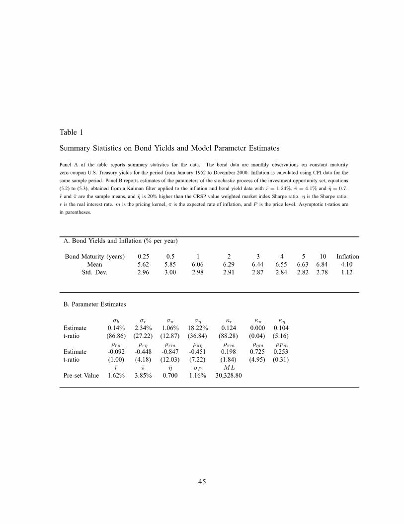
Table 1

Summary Statistics on Bond Yields and Model Parameter Estimates

Panel A of the table reports summary statistics for the data. The bond data are monthly observations on constant maturity

zero coupon U.S. Treasury yields for the period from January 1952 to December 2000. Inflation is calculated using CPI data for the

same sample period. Panel B reports estimates of the parameters of the stochastic process of the investment opportunity set, equations

(5.2) to (5.3), obtained from a Kalman filter applied to the inflation and bond yield data with r = 1.24%, π = 4.1% and η = 0.7.

r and π are the sample means, and η is 20% higher than the CRSP value weighted market index Sharpe ratio. η is the Sharpe ratio.

r is the real interest rate. m is the pricing kernel, π is the expected rate of inflation, and P is the price level. Asymptotic t-ratios are

in parentheses.

A. Bond Yields and Inflation (% per year)

Bond Maturity (years) 0.25 0.5 1 2 3 4 5 10 Inflation

Mean 5.62 5.85 6.06 6.29 6.44 6.55 6.63 6.84 4.10

Std. Dev. 2.96 3.00 2.98 2.91 2.87 2.84 2.82 2.78 1.12

B. Parameter Estimates

σb σr σπ ση κr κπ κη

Estimate 0.14% 2.34% 1.06% 18.22% 0.124 0.000 0.104

t-ratio (86.86) (27.22) (12.87) (36.84) (88.28) (0.04) (5.16)

ρrπ ρrη ρrm ρπη ρπm ρηm ρPm

Estimate -0.092 -0.448 -0.847 -0.451 0.198 0.725 0.253

t-ratio (1.00) (4.18) (12.03) (7.22) (1.84) (4.95) (0.31)

r π η σP MLPre-set Value 1.62% 3.85% 0.700 1.16% 30,328.80

45

Table 2

The Market Dividend Yield and the State Variables

The table reports the results of regressing the log dividend yield, y ≡ ln (x/V ), on the real interest rate, r, the expected

rate of inflation, π, the Sharpe ratio, η, and the expected long-term growth rate in earnings, g. Panel A reports the results of ADF

unit root tests. Panels B and C report the normalized cointegrating coefficients. Standard errors are adjusted for heteroskedasticity

and serial correlation using the Newey-West correction. *: significant at 1% level. **: significant at 5% level.

Panel A: Augmented Dickey-Fuller Test

r π η g DYAutocorrelation 0.949 0.954 0.952 0.980 0.981

ADF Test Statistic -2.49 -2.08 -3.02∗∗ 1.34 0.27

ADF on the First Difference -7.28∗ -11.26∗ -7.65∗ -4.83∗ -6.58∗

Panel B: Normalized Cointegrating Coefficients including π

y Constant r π η g LLCointegration Coefficient 1.00 4.02 -2.04 -28.36∗ -0.48∗ 6.77∗ 3360.44

Asymptotic Std. Error 1.83 4.92 0.10 2.36

Panel C: Normalized Cointegrating Coefficients excluding π

y Constant r π η g LLCointegration Coefficient 1.00 3.06 -14.71∗ -0.55∗ 10.64∗ 2451.17

Asymptotic Std. Error 4.95 0.20 4.00

46

Table 3

FF Portfolio Returns and Innovations in the State Variable Estimates

Panel B reports regressions of innovations in r, π, and η on the Fama-French portfolio returns. The innovation, εr(t), is

calculated using the following expression:

1

σr

[rt − r

(1 − e−κr/12

)− rt−1e

−κr/12]

The innovations, επ(t) and εη(t) are similarly defined. The t-ratios, reported in parentheses, are calculated using the Newey-West

adjustment for heterogeneity and serial correlation.

A. Innovations in the State Variable Estimates vs. FF Portfolio Returns

Dependent Const. Rm − Rf SMB HML Adj. R2 S.E.

Variables

1. εr 0.0179 -0.856 0.283 -1.153 0.0162 0.268

(1.60) (2.87) (0.73) (2.26)

2. επ 0.009 -0.869 0.213 0.161 0.0054 0.363

(0.52) (1.85) (0.41) (0.27)

3. εη -0.028 0.541 2.077 2.256 0.0255 0.429

(1.14) (0.85) (3.35) (2.56)

B. FF Portfolio Returns vs. Innovations in the State Variable Estimates

Dependent Const. εr επ εη Adj. R2 S.E.

Variables

1. Rm − Rf 0.007 -0.041 -0.010 -0.035 0.0443 0.041

(3.66) (4.32) (4.10) (1.63)

2. SMB 0.001 0.012 0.012 0.013 0.0184 0.029

(0.82) (2.04) (2.40) (3.28)

3. HML 0.004 -0.002 0.008 0.007 0.0114 0.027

(2.86) (0.43) (1.55) (2.22)

47

Table 4

Regressions of HML and SMB Portfolio Returns on Market Returns and StateVariable Innovations

This table reports regressions of monthly HML and SMB portfolio returns on market excess returns (Rm − Rf ) and esti-

mated innovations in the real interest rate ∆r, and the Sharpe ratio, ∆η for the period January 1952 to December 2000. The t-ratios,

reported in parentheses, are calculated using the Newey-West adjustment for heterogeneity and serial correlation.

Dep. Variable Const. Rm − Rf ∆η ∆r R2

Panel A: Whole sample January 1952 to December 2000

(1) HML 0.504% -0.221 12.00%

(3.96) (5.90)

(2) HML 0.524% -0.230 0.034 -0.460 13.85%

(4.09) (6.29) (2.29) (2.59)

(3) SMB -0.609% 0.174 6.05%

(0.05) (4.91)

(4) SMB 0.129% 0.175 0.040 0.226 7.15%

(0.01) (5.07) (2.89) (1.35)

Panel B: Sub-sample January 1952 to June 1976

(5) HML 0.433% -0.061 0.87%

(2.97) (1.06)

(6) HML 0.447% -0.076 0.050 -0.355 2.64%

(2.96) (1.35) (2.00) (1.47)

(7) SMB -0.046% 0.189 8.02%

(0.28) (3.48)

(8) SMB 0.035% 0.177 0.057 -0.014 9.11%

(0.22) (3.40) (2.07) (0.05)

Panel C: Sub-sample July 1976 to December 2000

(5) HML 0.580% -0.358 26.11%

(2.86) (6.84)

(6) HML 0.599% -0.365 0.018 -0.545 27.58%

(2.99) (6.92) (1.00) (2.56)

(7) SMB 0.034% 0.162 4.50%

(0.19) (3.40)

(8) SMB 0.043% 0.169 0.034 0.345 5.38%

(0.24) (3.65) (2.12) (1.69)

48

Table 5

Tracking Portfolios for Innovations in r and η

Panel A reports two sets of estimates of tracking portfolios for the yield-based estimates of the innovations in r and η for

the sample period from January 1952 to December 2000. Variables XSG through XBV are excess returns on six size and

book-to-market sorted portfolios formed by Fama and French. r and η are the estimates of the estimated real interest rate and the

maximum Sharpe ratio.

Panel B reports the correlations among HML, SMB, ∆η, ∆r, and the returns on the r and η tracking portfolios, Rr and Rη .

The t-ratios, reported in parentheses, are calculated using the Newey-West adjustment for heterogeneity and serial correlation.

A. Tracking Portfolio Composition

Dep. Var. C XSG XSN XSV XBG XBN XBV η−1 R2

(1) ∆r 0.000 0.035 -0.046 -0.004 0.003 -0.026 0.007 1.73%

(1.62) (1.52) (1.14) (0.15) (0.14) (1.01) (0.42)

(2) ∆r 0.000 0.038 -0.049 -0.004 0.001 -0.026 0.008 0.001 1.92%

(0.06) (1.52) (1.42) (0.15) (0.05) (0.98) (0.44) (0.99)

(3) ∆r -0.645 -0.460 0.561 0.410 0.102 -0.472 0.023 3.07%

(1.45) (1.95) (1.15) (1.29) (0.62) (1.96) (0.11)

(4) ∆r 0.000 -0.500 0.609 0.411 0.127 -0.482 -0.029 -0.015 3.41%

(0.01) (2.08) (1.21) (1.28) (0.81) (1.99) (0.14) (0.87)

B. Correlations

HML SMB ∆η ∆r Rη Rr

HML 1.00

SMB -0.26 1.00

∆η 0.08 0.12 1.00

∆r -0.08 0.03 0.01 1.00

Rη 0.41 0.59 0.20 -0.06 1.00

Rr -0.43 0.16 -0.07 0.17 -0.34 1.00

49

Table 6

ICAPM Regressions for HML and SMB

This table reports the regressions of HML and SMB portfolio returns on the market risk premium, RM − Rf , and the

returns on the r and η tracking portfolios, Rr and Rη . The t-ratios, reported in parentheses, are calculated using the Newey-West

adjustment for heterogeneity and serial correlation. In Panels B and C, lines with odd numbers use tracking portfolios formed for the

sub-period; and lines with even numbers use tracking portfolios formed for the whole sample period.

Dep. Variable Const. Rm − Rf Rη Rr R2

Panel A: Whole sample January 1952 to December 2000

(1) HML 0.000% -0.458 0.515 -17.243 66.50%

(0.01) (20.51) (7.68) (12.49)

(2) SMB -0.152% 0.288 1.347 17.289 62.67%

(1.55) (7.23) (15.44) (6.85)

Panel B: Sub-sample January 1952 to June 1976

(3) HML 0.262% -0.243 0.732 -1.225 28.85%

(1.96) (4.34) (6.16) (0.74)

(4) HML 0.110% -0.386 0.631 -15.159 57.09%

(1.10) (10.90) (6.94) (9.88)

(5) SMB -0.276% -0.010 1.206 7.881 44.53%

(1.96) (0.19) (12.78) (5.15)

(6) SMB -0.203% 0.149 1.314 12.868 60.22%

(1.67) (2.50) (17.97) (6.66)

Panel C: Sub-sample July 1976 to December 2000

(7) HML 0.022% -0.551 -0.041 14.762 66.78%

(0.19) (16.57) (0.45) (12.44)

(8) HML -0.136% -0.519 0.436 -19.917 78.51%

(1.71) (23.10) (7.76) (15.66)

(9) SMB 0.093% 0.486 1.437 17.791 73.52%

(0.82) (9.73) (13.11) (7.50)

(10) SMB 0.001% 0.345 0.867 13.247 46.93%

(0.01) (6.77) (9.09) (3.31)

50

Table 7

Risk Premium Estimates for the HML and SMB Portfolios

Panel A of the table reports the estimated risk premium, the standard deviation of excess returns and the t-statistic for the

risk premium for the market portfolio and for the r, π and η tracking portfolios. The sample period is from February 1952 to

December 2000 with 588 observations. Panel B of the table reports for HML and SMB the sample mean excess returns, and the

breakdowns of the ICAPM tracking portfolio estimates of the risk premia.

Panel A: Summary Statistics of the r, π, and η Tracking Portfolios

Zero-Investment r Tracking η Tracking π Tracking

Market Portfolio Portfolio Portfolio Portfolio

(1) Mean Excess Return 7.40% -0.31% 4.68% -0.11%

(2) S.D. of Excess Return 14.65% 0.36% 5.53% 0.17%

(3) t-ratio for Mean Excess Return 3.54 6.06 5.94 4.33

Panel B: Risk Premia Breakdowns for the HML and SMB Portfolios

Sample Rm − Rf Rr Rη Total

Mean

(1) HML 4.41% -3.39% 5.38% 2.41% 4.40%

(2) SMB 1.22% 2.13% -5.39% 6.32% 3.06%

51

Table 8

ICAPM Regressions for 25 Portfolios with Tracking Portfolios

This table reports the regressions of the excess returns on 25 size and book-to-market sorted portfolios on the market risk

premium, RM − Rf , and the returns on the r and η tracking portfolios, Rr and Rη . The t-ratios are calculated using the

Newey-West adjustment for heterogeneity and serial correlation. The sample period is from January 1952 to December 2000.

Size Book-to-Market Book-to-Market

Low 2 3 4 High Low 2 3 4 High

α(%) t(α)small -0.50 -0.18 -0.19 -0.03 -0.06 2.58 1.20 1.52 0.25 0.65

2 -0.26 -0.23 -0.10 -0.10 -0.12 2.06 2.13 1.21 1.18 1.34

3 -0.08 -0.11 -0.22 -0.07 -0.14 0.79 1.23 2.84 0.89 1.67

4 0.07 -0.23 -0.08 -0.04 -0.12 0.72 2.78 1.12 0.60 1.20

big 0.13 -0.03 0.07 -0.08 -0.08 1.79 0.55 1.31 0.95 0.71

βmkt t(βmkt)small 1.63 1.35 1.12 1.00 0.99 22.68 19.32 21.96 28.53 33.32

2 1.61 1.21 0.97 0.90 0.98 27.58 25.17 25.95 33.37 30.88

3 1.52 1.05 0.87 0.79 0.87 41.03 30.48 25.06 23.58 21.60

4 1.37 0.99 0.84 0.80 0.88 38.43 26.45 26.89 25.17 19.53

big 1.10 0.88 0.72 0.66 0.70 37.42 37.39 34.89 17.69 12.75

βη t(βη)small 1.66 1.77 1.67 1.67 1.94 9.83 12.23 14.42 20.47 20.46

2 0.97 1.19 1.20 1.24 1.57 9.50 15.12 18.41 19.80 21.48

3 0.74 0.70 0.77 0.84 1.23 9.28 10.74 16.04 14.17 16.10

4 0.25 0.18 0.31 0.55 0.87 3.36 2.92 4.37 9.12 7.78

big -0.19 -0.44 -0.62 -0.14 0.35 3.71 7.87 9.83 1.64 2.91

βr t(βr)small 33.15 22.88 13.54 9.27 8.19 8.55 5.10 4.70 5.27 6.17

2 26.37 11.09 2.45 -0.51 2.41 9.05 5.17 1.43 0.40 1.91

3 22.52 1.11 -5.63 -7.11 -3.51 10.43 0.62 3.65 3.81 1.63

4 14.91 -5.04 -10.27 -7.94 -6.85 6.03 3.19 5.79 5.63 2.41

big 5.18 -9.96 -16.00 -16.43 -10.57 3.21 7.59 24.75 7.78 3.72

52

Table 8.1

ICAPM Regressions for 25 Portfolios with Tracking Portfolios: January 1952 toJune 1976

This table reports the regressions of the excess returns on 25 size and book-to-market sorted portfolios on the market risk

premium, RM − Rf , and the returns on the r and η tracking portfolios, Rr and Rη . The t-ratios are calculated using the

Newey-West adjustment for heterogeneity and serial correlation. The sample period is from January 1952 to June 1976.

Size Book-to-Market Book-to-Market

Low 2 3 4 High Low 2 3 4 High

α(%) t(α)Small -0.53 -0.34 -0.32 -0.04 0.00 2.24 1.84 2.05 0.31 0.01

2 -0.35 -0.24 -0.04 -0.08 0.06 1.99 1.74 0.30 0.77 0.52

3 -0.15 -0.08 -0.09 0.12 -0.13 1.12 0.67 0.84 1.30 0.92

4 -0.09 -0.22 0.15 0.06 -0.01 0.80 1.90 1.72 0.66 0.09

Big 0.11 -0.05 0.15 -0.02 -0.03 1.35 0.81 2.11 0.13 0.17

βmkt t(βmkt)Small 1.35 1.17 0.94 0.91 0.88 12.23 11.18 11.71 14.45 20.41

2 1.50 1.13 0.91 0.88 0.94 13.62 12.87 12.57 18.24 13.84

3 1.43 0.99 0.89 0.82 0.86 18.30 16.31 12.60 16.92 14.63

4 1.32 0.98 0.83 0.84 0.98 25.03 14.81 18.14 17.98 13.92

Big 1.18 0.86 0.68 0.74 0.82 30.29 37.36 26.45 18.49 8.57

βη t(βη)Small 1.84 1.83 1.80 1.78 2.20 10.50 13.79 16.25 17.58 24.58

2 1.01 1.24 1.30 1.26 1.69 7.86 10.93 12.41 15.73 17.21

3 0.73 0.72 0.76 0.96 1.39 8.88 7.58 10.22 11.74 11.84

4 0.19 0.20 0.30 0.67 1.16 2.63 2.68 2.82 7.43 8.19

Big -0.17 -0.28 -0.49 -0.03 0.53 3.24 4.78 9.00 0.36 2.74

βr t(βr)Small 22.84 14.81 7.87 5.75 6.84 6.17 4.32 2.97 2.76 4.04

2 24.84 10.88 4.07 -0.69 2.80 7.32 3.73 1.61 0.40 1.24

3 19.44 2.91 -3.05 -3.83 0.33 7.62 1.38 1.85 2.36 0.16

4 13.05 -3.22 -7.93 -6.29 -0.38 7.53 1.51 4.61 3.26 0.15

Big 8.80 -6.84 -16.63 -13.83 5.94 6.22 7.11 17.73 9.28 1.96

53

Table 8.2

ICAPM Regressions for 25 Portfolios with Tracking Portfolios: July 1976 to De-cember 2000

This table reports the regressions of the excess returns on 25 size and book-to-market sorted portfolios on the market risk

premium, RM − Rf , and the returns on the r and η tracking portfolios, Rr and Rη . The t-ratios are calculated using the

Newey-West adjustment for heterogeneity and serial correlation. The sample period is from July 1976 to December 2000.

Size Book-to-Market Book-to-Market

Low 2 3 4 High Low 2 3 4 High

α(%) t(α)Small -0.47 -0.01 -0.05 0.00 -0.11 1.61 0.06 0.31 0.01 0.73

2 -0.21 -0.25 -0.21 -0.11 -0.30 1.15 1.53 1.73 0.89 2.44

3 -0.02 -0.21 -0.38 -0.25 -0.17 0.14 1.46 3.75 2.14 1.70

4 0.21 -0.27 -0.37 -0.11 -0.16 1.29 2.29 3.60 1.06 1.40

Big 0.17 0.00 0.01 -0.12 -0.08 1.49 0.05 0.13 0.87 0.47

βmkt t(βmkt)Small 1.77 1.44 1.21 1.04 1.03 24.44 18.30 22.58 27.90 29.58

2 1.69 1.26 1.02 0.90 1.00 27.53 24.91 28.05 29.62 37.43

3 1.58 1.11 0.88 0.77 0.87 43.35 29.31 25.92 19.04 17.50

4 1.41 1.02 0.87 0.75 0.79 31.28 26.71 22.75 17.97 15.28

Big 1.05 0.88 0.73 0.59 0.61 34.13 30.03 27.92 12.26 9.08

βη t(βη)Small 1.58 1.75 1.63 1.59 1.75 6.38 8.10 9.43 13.88 13.10

2 1.04 1.23 1.19 1.24 1.50 6.59 10.75 13.68 12.55 13.70

3 0.78 0.79 0.83 0.74 1.12 6.14 7.62 12.06 8.30 10.34

4 0.34 0.22 0.38 0.40 0.54 2.79 2.22 3.84 4.50 3.61

Big -0.25 -0.55 -0.74 -0.30 0.09 3.12 7.78 6.96 2.35 0.57

βr t(βr)Small 38.00 26.94 16.26 10.88 8.42 8.10 4.49 4.32 4.80 4.60

2 27.10 11.07 1.36 -0.45 1.85 6.67 3.81 0.61 0.26 1.18

3 24.08 0.06 -7.08 -9.08 -5.69 8.40 0.03 3.67 3.97 2.17

4 16.05 -6.04 -11.73 -8.96 -10.51 4.61 3.05 5.02 4.95 -3.45

Big 3.38 -11.75 -15.93 -17.80 -13.06 1.83 7.85 21.83 6.80 3.99

54

Table 9

ICAPM Regressions for 25 Portfolios with Fama-French Factors: January 1952 toDecember 2000

This table reports the regressions of the excess returns on 25 size and book-to-market sorted portfolios on the market risk

premium, RM −Rf , and the returns on SMB and HML portfolios. The t-ratios are calculated using the Newey-West adjustment

for heterogeneity and serial correlation. The sample period is from January 1952 to December 2000.

Size Book-to-Market Book-to-Market

Low 2 3 4 High Low 2 3 4 High

α(%) t(α)Small -0.44 -0.05 0.00 0.15 0.11 3.39 0.59 0.02 3.13 2.14

2 -0.23 -0.09 0.08 0.06 0.02 3.17 1.53 1.33 1.13 0.36

3 -0.03 0.02 -0.07 0.04 -0.06 0.58 0.28 1.01 0.61 1.00

4 0.09 -0.16 -0.01 0.00 -0.11 1.18 2.08 0.08 0.04 1.32

Big 0.15 -0.04 0.03 -0.15 -0.20 2.78 0.73 0.36 2.51 2.62

βmkt t(βmkt)Small 1.06 1.00 0.94 0.93 0.99 35.28 40.82 62.38 60.89 54.79

2 1.11 1.03 0.98 0.99 1.08 55.91 62.11 53.30 75.66 61.39

3 1.09 1.03 1.02 1.01 1.08 60.96 44.94 39.74 61.49 47.27

4 1.05 1.07 1.05 1.02 1.15 57.73 39.72 41.24 47.98 41.32

Big 0.99 1.02 0.97 1.02 1.05 53.95 53.63 40.87 59.86 37.43

βSMB t(βSMB)Small 1.43 1.31 1.13 1.04 1.09 33.68 22.78 41.33 38.79 26.99

2 1.02 0.88 0.75 0.70 0.82 28.53 20.10 15.42 26.45 26.90

3 0.74 0.53 0.44 0.40 0.53 26.45 7.65 6.62 8.07 9.71

4 0.39 0.20 0.16 0.23 0.29 9.95 3.32 2.58 7.73 4.66

Big -0.26 -0.24 -0.26 -0.22 -0.06 10.04 6.77 7.81 8.23 1.71

βHML t(βHML)Small -0.19 0.13 0.30 0.47 0.70 2.92 2.45 11.04 18.34 19.28

2 -0.36 0.15 0.38 0.57 0.74 8.68 2.99 7.22 14.55 24.20

3 -0.41 0.18 0.46 0.65 0.83 15.14 2.76 7.21 11.24 17.44

4 -0.42 0.19 0.45 0.60 0.84 10.92 2.77 6.99 13.40 17.70

Big -0.37 0.09 0.25 0.65 0.87 11.52 1.85 5.63 15.09 21.03

55

Table 9.1

ICAPM Regressions for 25 Portfolios with Fama-French Factors: January 1952 toJune 1976

This table reports the regressions of the excess returns on 25 size and book-to-market sorted portfolios on the market risk

premium, RM −Rf , and the returns on SMB and HML portfolios. The t-ratios are calculated using the Newey-West adjustment

for heterogeneity and serial correlation. The sample period is from January 1952 to June 1976.

Size Book-to-Market Book-to-Market

Low 2 3 4 High Low 2 3 4 High

α(%) t(α)Small -0.31 -0.14 -0.11 0.14 0.17 1.60 1.21 1.26 2.54 2.91

2 -0.20 -0.08 0.14 0.02 0.15 1.75 0.92 1.93 0.33 1.74

3 -0.01 0.05 0.02 0.17 -0.11 0.09 0.57 0.29 2.39 1.15

4 -0.01 -0.17 0.17 0.06 -0.06 0.14 1.61 2.09 0.80 0.58

Big 0.13 -0.09 0.09 -0.15 -0.22 1.90 1.26 1.03 2.01 2.00

βmkt t(βmkt)Small 1.05 1.04 0.93 0.95 0.98 20.98 31.57 41.37 62.48 34.54

2 1.09 1.01 0.93 1.00 1.07 34.53 46.10 40.34 55.62 44.23

3 1.11 0.96 0.98 0.99 1.02 44.52 42.43 27.99 46.03 46.45

4 1.08 1.00 0.98 1.02 1.14 44.60 30.50 38.64 41.04 33.50

Big 1.04 0.95 0.89 1.01 1.04 44.14 40.86 28.17 47.83 21.59

βSMB t(βSMB)Small 1.49 1.27 1.19 1.11 1.20 19.11 27.45 23.86 40.06 33.97

2 1.09 0.96 0.87 0.74 0.87 17.74 18.45 26.20 24.58 29.83

3 0.78 0.62 0.54 0.48 0.66 16.51 16.07 13.05 12.78 20.70

4 0.36 0.30 0.22 0.32 0.48 7.19 5.80 4.67 8.54 7.66

Big -0.19 -0.15 -0.20 -0.21 0.01 6.35 3.98 5.09 5.70 0.17

βHML t(βHML)Small 0.02 0.25 0.38 0.49 0.74 0.18 4.14 8.55 17.18 14.73

2 -0.35 0.09 0.27 0.53 0.73 6.42 1.75 5.89 20.53 17.95

3 -0.38 0.07 0.30 0.55 0.78 10.00 1.39 5.85 13.53 20.45

4 -0.38 0.09 0.35 0.57 0.80 8.60 1.70 6.20 12.32 15.26

Big -0.39 0.10 0.28 0.64 0.89 12.21 2.35 7.72 14.76 12.86

56

Table 9.2

ICAPM Regressions for 25 Portfolios with Fama-French Factors: July 1976 toDecember 2000

This table reports the regressions of the excess returns on 25 size and book-to-market sorted portfolios on the market risk

premium, RM −Rf , and the returns on SMB and HML portfolios. The t-ratios are calculated using the Newey-West adjustment

for heterogeneity and serial correlation. The sample period is from July 1976 to December 2000.

Size Book-to-Market Book-to-Market

Low 2 3 4 High Low 2 3 4 High

α(%) t(α)Small -0.55 0.06 0.12 0.20 0.09 3.70 0.59 1.55 2.49 1.08

2 -0.24 -0.09 0.04 0.12 -0.10 2.82 1.07 0.44 1.38 1.40

3 -0.03 -0.01 -0.15 -0.07 0.00 0.41 0.14 1.61 0.76 0.01

4 0.20 -0.16 -0.20 -0.03 -0.09 1.82 1.50 1.99 0.35 0.87

Big 0.23 0.00 -0.06 -0.16 -0.16 2.68 0.04 0.52 1.63 1.52

βmkt t(βmkt)Small 1.02 0.94 0.92 0.89 0.97 34.97 34.71 50.16 36.11 41.79

2 1.11 1.06 1.03 0.97 1.09 44.08 47.15 46.30 48.58 47.25

3 1.05 1.11 1.07 1.03 1.13 43.7 33.13 31.91 39.94 36.46

4 1.02 1.14 1.14 1.01 1.13 38.90 34.91 31.85 29.32 32.21

Big 0.92 1.09 1.03 1.04 1.04 40.73 49.40 35.86 35.44 30.20

βSMB t(βSMB)Small 1.34 1.29 1.06 0.96 1.01 24.57 17.23 35.13 26.41 19.65

2 0.97 0.83 0.69 0.68 0.79 23.16 18.03 14.01 19.42 19.75

3 0.70 0.50 0.42 0.37 0.46 19.65 5.79 5.39 5.90 7.20

4 0.39 0.17 0.16 0.16 0.15 7.91 2.27 2.00 3.70 2.31

Big -0.33 -0.30 -0.29 -0.23 -0.12 10.69 7.12 5.63 6.48 3.36

βHML t(βHML)Small -0.38 0.01 0.22 0.40 0.63 5.04 0.14 6.34 10.32 12.94

2 -0.39 0.18 0.45 0.58 0.74 6.69 2.62 6.53 9.66 20.39

3 -0.47 0.28 0.57 0.70 0.85 13.21 3.28 7.07 8.31 13.60

4 -0.47 0.26 0.55 0.58 0.79 8.24 2.79 6.25 8.23 12.61

Big -0.43 0.10 0.25 0.65 0.81 9.82 1.40 3.52 9.94 15.13

57

Table 9.2

ICAPM, FF and CAPM Regressions for 30 Industrial Portfolios: January 1952 toDecember 2000

This table reports the GRS test statistics and the intercepts α in individual regressions of the excess returns on 30 indus-

trial portfolios on the market risk premium, RM −Rf under CAPM, the returns on RM −Rf , SMB and HML portfolios under

FF, and returns on RM − Rf , Rη and Rr under the ICAPM. The tracking portfolio returns of Rr and Rη are formed using the

30 industrial portfolios. The t-ratios are calculated using the Newey-West adjustment for heterogeneity and serial correlation. The

sample period is from January 1952 to December 2000.

Industry ICAPM FF CAPM

α(%) t(α) α(%) t(α) α(%) t(α)Food 0.24 1.98 0.20 1.56 0.27 2.03

Beer 0.17 1.11 0.02 0.12 0.14 0.84

Smoke 0.47 1.99 0.44 1.80 0.54 2.20

Games 0.08 0.40 0.03 0.15 0.02 0.12

Books 0.16 1.12 0.06 0.42 0.13 0.89

Hshld 0.19 1.59 0.25 2.18 0.17 1.47

Clths -0.13 0.67 -0.43 2.42 -0.18 0.92

Hlth 0.25 1.73 0.47 3.35 0.30 2.06

Chems -0.04 0.36 -0.23 1.95 -0.09 0.74

Txtls -0.03 0.18 -0.48 2.90 -0.17 0.91

Cnstr -0.11 1.03 -0.28 2.62 -0.12 1.10

Steel -0.18 1.22 -0.35 3.75 -0.29 1.80

FabPr -0.12 1.05 -0.23 1.98 -0.16 1.31

ElcEq 0.09 0.55 0.23 1.41 0.05 0.32

Autos 0.07 0.44 -0.26 1.72 0.01 0.07

Carry 0.11 0.58 -0.02 0.10 0.14 0.70

Mines -0.14 0.63 -0.39 1.74 -0.23 1.04

Coal 0.02 0.09 -0.25 0.86 -0.06 0.20

Oil 0.13 0.86 0.03 0.22 0.17 1.05

Util 0.08 1.03 -0.02 0.15 0.20 1.55

Telcm 0.12 0.81 0.18 1.29 0.17 1.10

Servs 0.13 0.79 0.30 2.40 0.08 0.49

BusEq 0.19 1.19 0.40 2.80 0.15 0.92

paper -0.04 0.34 -0.13 1.16 -0.02 0.20

Trans -0.12 0.79 -0.39 3.09 -0.14 0.98

Whlsl 0.00 0.02 -0.08 0.76 -0.04 0.32

Rtail 0.14 1.10 0.07 0.50 0.10 0.72

Meals 0.10 0.49 -0.03 0.14 0.08 0.39

Fin 0.02 0.17 -0.10 0.98 0.08 0.76

Other -0.18 1.26 -0.25 1.64 -0.16 1.09

GRS F-statistic 1.39 3.00 1.52

p−value 0.083 < 0.01 0.039

58

Figure 1

Time Series of Real Interest Rate Estimates

The figure plots the estimated real interest rate series from January 1952 to December 2000, which is filtered out from the bond

yield and inflation data. Shaded area indicates periods of U.S. recessions.

1952.01 1957.01 1962.01 1967.01 1972.01 1977.01 1982.01 1987.01 1992.01 1997.01−0.05

0

0.05

0.1

0.15

59

Figure 2

Time Series of Sharpe Ratio Estimates

The figure plots the estimated Sharpe ratio series from January 1950 to December 2000, which are filtered out from the bond yield

and inflation data. Shaded area indicates periods of U.S. recessions.

1952.01 1957.01 1962.01 1967.01 1972.01 1977.01 1982.01 1987.01 1992.01 1997.01−1.5

−1

−0.5

0

0.5

1

1.5

2

2.5

60