NBER WORKING PAPERS SERIES

INTERTEMPORAL ASSET PRICING WITHOUT CONSUMPTION DATA

John Y. Campbell

Working Paper No. 3989

NATIONAL BUREAU OF ECONOMIC RESEARCH1050 Massachusetts Avenue

Cambridge, MA 02138February 1992

I am grateful to the LSE Financial Markets Group for its hospitality during th academic year1989-90. to the National Science Foundation and the Sloan Foundation for financial support,and to Kevin Carey and Hyeng Keun Koo for able research assistance. Andrew Abel, FischerBlack, Doug Breeden, Steve Cecchetti, John Cochrane, George Constantinides, SilverioForesi, Ravi Jagannathan. Bob Merton, Lars Svensson, Philippe Well, Steve Zeldes, and tworeferees made helpful comments on earlier drafts, which canied the title "Intertemporal AssetPricing Without Consumption. This paper is part of NBER's research programs in AssetPricing and Economic fluctuations. Any opinions expressed are those of the author and notthose of the National Bureau of Economic Research.

NBER Working Paper #3989February 1992

INTERTEMPORAL ASSET PRICING WIThOUT CONSUMPTION DATA

ABSTRACT

This paper proposes a new way to generalize the insights of static asset pricing theory

to a multi-period setting. The paper uses a loglinear approximation to the budget constraint

to substitute out consumption from a standard intertemporal asset pricing model. In a

homoskedastic lognormal setting, the consumption-wealth ratio is shown to depend on the

elasticity of intertemporal substitution in consumption, while asset risk premia are determined

by the coefficient of relative risk aversion. Risk premia are related to the covariances of asset

returns with the market return and with news about the discounted value of all future market

returns.

John Y. CampbellWoodrow Wilson SchoolPrinceton UniversityPrinceton, NJ 08544-1013and NBER

1. Introduction

For the last twenty years an important goal of financial research has been to

generalize theinsights of the simple one-period Capital Asset Pricing Model (CAPM)to a multi-period setting. Such a generalization is difficult to achieve because the multi-

period consumption and portfolio choice problem is inherently nonlinear. A compictcsolution is obtained by combining the consumer's Euler equation with the interteinporal

budget constraint, but the budget constraint is a nonlinear equation except in veryspecial cases.

In response to this difficulty Merton (1969, 1971, 1973) suggested reformulatingthe consumption and portfolio choice problem in continuous time. Doing this in effect

linearizes by taking the decision interval as infinitely small, so that the model becomeslinear over this interval. But this kind of linearity is only local, so it does not allow

one easily to study longer-run aspects of interternporai asset pricing theory.In this paper I take a different approach. Instead of assuming that the time

interval is small, I assume that variation in the consumption-wealth ratio is small.

This makes the intertemporal budget constraint approximately loglinear, allowing meto solve the consumption and portfolio choice problem in closed form. My approachclarifies the relation between the time-series properties of market returns and the time-

series properties of consumption. It also leads to a simple expression relating assets'

risk premia to their covariances with the market return and news about future market

returns. This formula unifies the large body of research on time-series properties ofaggregate stock returns with the equally large literature on cross-sectional patterns ofmean returns.

The formula for risk premia derived in this paper can be tested without using data

on consumption. This is potentially an important advantage, for empirical work usingaggregate consumption data has generally rejected the model restrictions or has esti-

mated implausible parameter values. These problems occur both with a simple power

specification for utility (Hansen and Singleton 1982, 1983, Mehra and Prescott 1985,Mankiw and Shapiro 1986) and with more elaborate specifications that allow for habit

formation (Constantinides 1990, Ferson and Constantinides 1991) or for a divergence

between the coefficient of relative risk aversion and the elasticity of intertemporal sub-

stitution (Epstein and Zin 1989, 1991, Giovannini and Jorion 1989, Weil 1987, 1989).

The difficulty may well be inherent in the use of aggregate consumption data. These

—1—

data are measured with error and are time aggregated, which can have serious con-

sequences for asset pricing relationships (Breeden, Gibbons, and Litzenberger 1989,Grossman, Melino, and Shiller 1987, Heaton 1990, Wheatley 1989, Wilcox 1989). More

fundamentally, the consumption of asset market participants may be poorly proxied by

aggregate consumption. Predictable movements in aggregate consumption growth arecorrelated with predictable growth in current disposable income, which suggests that

a large fraction of the population is liquidity-constrained or fails to optimize intertem-

porally (Campbell and Manlciw 1989), and micro evidence shows that the consumption

of stockholders behaves differently from the consumption of non-stockholders (Mankiw

and Zeldes 1991).

Of course, the approach of this paper does not resolve all measurement issues. The

formula for risk premia derived here requires that one be able to measure the return on

the market portfolio, which should in general include human capital. The difficulties

with this have been forcefully pointed out by Roll (1977) in his critique of tests ofthe static CAPM. But at the very least the results of the paper enable one to use theimperfect data on both market returns and consumption in new and potentially fruitful

ways.

The next section of this paper shows how to obtain a loglinear approximation to

the intertemporal budget constraint. Section 3 develops implications for asset pric-ing when asset returns are jointly lognormal and homoskedastic, and when consumers

have the objective function proposed by Epstein and Zin (1989, 1990) and Weil (1987).This objective function implies that the consumption-wealth ratio is constant when-ever the intertemporal elasticity of substitution is equal to one, so it provides a natural

benchmark case in which the loglinear approximation of this paper holds exactly. Im-

portantly, the intertemporal asset pricing model differs from a one-period asset pricing

model even in this benchmark case. This section of the paper derives several alternative

expressions for risk premia and discusses how they might be tested empirically. Section

4 allows for changing second moments of asset returns. Section 5 assesses the accuracy

of the approximation to the intertemporal budget constraint, and section 6 concludes.

—2—

2. A Loglinear Approximation to the Intertemporal Budget Constraint

I consider a representative agent economy in which all wealth, including humancapital, is tradable. I define Wj to be total wealth, including human capital, at the

beginning of period t, Cj to be consumption at time ,and Rmg+i to be the gross simplereturn on wealth invested from period I to period I + 1. The subscript m denotes thefact that total invested wealth is the "market portfolio" of assets. The representative

agent's dynamic budget constraint can then be written as

= Rm,t+i (W — Ct). (2.1)

Labor income does not appear explicitly in this budget constraint because of the as-sumption that the market value of tradable human capital is included in wealth. The

budget constraint can be solved forward, imposing a condition that the limit of dis-counted future wealth is zero, to obtain the highly nonlinear present value budgetconstraint

W = Cj+ . (2.2)1=1 (n)1

The loglinear approximation begins by dividing (2.1) through by Wi, to obtain

____ ,' C 23= Rm,e+it1 —

or in logs (indicated by lower-case letters)

Awg+i = rmj+1 + log(1 —exp(ct — wg)). (2.4)

The second term on the right hand side is a nonlinear function of the log consumption-

wealth ratio. Consider this as a function of some variable xj = log(Xj), and take afirst-order Taylor expansion around the mean The resulting approximation is

—3—

log(l — exp(xj)) log(1 — exp(2)) —1 (_)(Xi

— (2.5)

If xj is a constant x = log(X), then the coefficient —exp(i)/(1 — exp(±)) equals— X). In the present application, when the log consumption-wealth ratio is

a constant the coefficient equals —C/(W— C), the constant ratio of consumption to in-

vested wealth. Of course, when zg is random then by Jensen's Inequality the coefficient

no longer equals the average ratio of consumption to invested wealth.

Figures 1 and 2 give a visual impression of the approximation (2.5). In each figure

the horizontal axis measures the consumption-weaith ratio, using a log scale. The ver-

tical axis measures the "net growth rate of wealth", that is the growth rate of wealth

less the market return Awj+i — rm,I+I. The solid line shows the exact relationship— rm,i+j = log(1 — exp(cj — wg)), while the dashed straight line shows the

approximation (2.5). These lines are plotted over a horizontal range three standarddeviations on either side of the mean log consumption-wealth ratio, where the standard

deviation of the log consumption-wealth ratio is calculated for an example calibrated

in section 5 below using equation (5.2). Figure 1 assumes that the consumer has an

elasticity of intertemporal substitution in consumption equal to 2 (or zero, since thestandard deviation of the log consumption-wealth ratio depends on the distance of this

elasticity from one), while Figure 2 assumes an elasticity of intertemporal substitution

equal to 4. In this example the approximation is clearly very accurate when the vari-

ability of the log consumption-wealth ratio is as low as implied by an elasticity of 2,

but much less accurate when the variability is as high as implied by an elasticity of 4.

Section 5 of the paper discusses approximation accuracy in greater detail.It will be helpful to rewrite the coefficient —exp(2)/(1 — exp(±)) in (2.5) as 1— i/p

where p 1—exp(2). When the log consumption-wealth ratio is constant, then p can be

interpreted as (W—C)/W, the constant ratio of invested wealth to total wealth. Putting

together (2.4) and (2.5), the approximation to the intertemporsi budget constraint is

tm,ti + Ac + (i — !)(c —Wi), (2.6)

where the constant Ac can be calculated directly from (2.5).

The next step is to use the trivial equality

—4—

= tkCg+1 + (c — tug) — (cg+l — wgi). (2.7)

Equating the left hand sides of (2.6) and (2.7), one obtains a difference equation in

the log consumption-wealth ratio, cg — tug. This can be solved forward, assuming that

lim1....,, pi(cj1 — =0, to yield

cg—wg = + 1p (2.8)

This equation is the loglinear equivalent of the nonlinear expression (2.2). It says that

a high consumption-wealth ratio today must be followed either by high returns oninvested wealth, or by low consumption growth. This holds simply by virtue of theintertemporal budget constraint; there is no model of optimal behavior in equation

(2.8).Equation (2.8) holds cx post, but it also holds cx ante; if one takes expectations

of (2.8) at time 2, the left hand side is unchanged and the right hand side becomes anexpected discounted value:

cg—wg = Ezp'(rm÷j—Acj+j) + 1'• (2.9)

Equation (2.9) can be substituted into (2.6) and (2.7) to obtain

— Ejcg1 =

(2.10)

Equation (2.10) says that an upward surprise in consumption today must correspond toan unexpected return on wealth today (the first term in the first sum on the right hand

—5—

side of the equation), or to news that future returns will be higher (the remaining terms

in the first sum), or to a downward revision in expected future consumption growth(the second sum on the right hand side). This is similar to the equation discussed inCampbell (1991a) for an arbitrary stock portfolio. Here consumption plays the role of

dividends in the earlier analysis; aggregate wealth can be thought of as an asset whose

dividends are equal to consumption. In the next section, a loglinear Euler equation

will be used to eliminate expected future consumption growth from the right hand side

of (2.10), leaving only current and expected future asset returns.

—6—

3. Intertemporal Asset Pricing with Constant Variances

In this section I explore asset pricing relationships assuming that the conditionaljoint distribution of asset returns and consumption is homoskedastic. This assump-tion is unrealistic, since there is strong evidence that asset return variances change

through time, but it simplifies the analysis considerably. In the next section I allow for

heterosicedasticity.

The loglinear approximate budget constraint of the previous section can be com-bined with a loglinear Euler equation. To obtain such an Euler equation, I furtherassume that the joint conditional distribution of asset returns and consumption is log-normal. Below I show that this is an approximate implication of the more fundamental

assumption that returns and news about future returns are jointly lognormal. The log-

normality assumption can also be relaxed if one is willing to work with a second-order

Taylor approximation to the Euler equation.1

Along with these distributional assumptions, I use the non-expected utility model

proposed by Epstein and Zin (1989, 1991) and Weil (1987) to generate a loglinear Euler

equation that distinguishes the coefficient of relative risk aversion and the elasticity of

intertemporal substitution. In the standard model of time-separable power utility,relative risk aversion is the reciprocal of the elasticity of intertempc,ral substitution,

but as we shall see these concepts play quite different roles in the asset pricing theory.

The non-expected utility model also allows intertemporal considerations to affect asset

prices even when the consumption-wealth ratio is constant, something which is not

possible with time-separable power utility.

1Conditional joint Iogncs,naIity and homo.kedasddty art also assumed by Hansen and Singleton (19). Note that con-ditional lognonnality don not imply tsncondjtia,aJ lo.cnmality unit., conditional expected returi are conMant throughtime. Constant expected retuns and unconditional lognonnality are assumed in Merton's (1969, 1971) continuous-timemodel, where .11 asset return, follow jeometric Brownian ,notio the assumption used here is weaker.

—7--

3.1. The Euler Equation for a Simple Non-Expected Utility Model

The objective function for a simple non-expected utility model is defined recursively

by

1_I _j__Ut = {(t_fl)c4 +

={(Ifl)c1i1 + s7)5}T. (3.1)

Here 7 15 the coefficient of relative risk aversion, a is the elasticity of intertemporal sub-

stitution, and 8 is defined, following Giovannini and Weil (1989), as 9 =(1 — )/(1 — 1).Note that in general the coefficient 6 can have either sign. Important special cases of the

model include the case where the coefficient of relative risk aversion 7 approaches one,

so that 0 approaches zero; the case where the elasticity of intertemporal substitutiona approaches one, so that 6 approaches infinity; and the case where y = 1/c, so that8 = 1. Inspection of (3.1) shows that this last case gives the standard time-separable

power utility function with relative risk aversion 7. When both and a equal one, theobjective function is the time-separable log utility function.

Epstein and Zin (1989, 1991) have established several important properties of this

objective function. First, when consumption is chosen optimally the value function

(the maximized objective function) is given by

cr—c 2V1 = maxUj = (1—$) — . (3.2)

The objective function (3.1) has been normalized so that the value function is linearly

homogeneous in wealth (for a given consumption-wealth ratio). It is conventional to

normalize the time-separable power utility function so that wealth appears in the value

function raised to the power 1 — , but the normalization in (3.1) turns out to beconvenient here. Naturally the normalization makes no difference to the solution of themodel.2

2Thc notation used here is similar to that in Epstein and Zin (1991). Howewr theirparazneterp corresponds to I —(1/e)

—8—

Second, the Euler equation corresponding to (3.1) can be written as

10 1 1—0

1 = E [{s(——) '} {+} i+]. (3.3)

For the market portfolio itself, this takes the simpler form

1 = (3.4)

These equations collapse to the familiar expressions for power utility when 8 = 1.When asset returns and consumption are jointly homoskedastic and lognormally

distributed, the Euler equations (3.3) and (3.4) can be rewritten in log form. Thisrewriting can also be justified as a second-order Taylor approximation if asset returns

and consumption are jointly homoskedastic. The log version of (3.4) takes the form

0 = 8logfi — + BEjrm1g+i + [()2vcc+e2vmm_vcm]. (3.5)

Here lower case letters are again used for logs. V4 denotes Var(act÷i), and otherexpressions of the form are defined in analogous fashion.

Equation (3.5) implies that there is a. linear relationship between expected con-sumption growth and the expected return on the market portfolio, with a slope coeffi-

dent equal to the intertemporal elasticity of substitution a. The relationship is

= pm + aEtr,i÷i,

Pm = clogf3 + [()Vcc+8avmm_2ovcm]

18 1= clogfi + 1(—)variact÷i — crmi÷l . (3.6)

here. Their paraneter a correspont to 1 —, here. Tb.. the parajnetE 0 here is p/cs in their notation. Note also thatthere are moe. in equations (10) through (12) of thefr paper. Equation (3.2) here ii acorrected version of their equation(12). Cionnnii,i and Well (1989) also give the correct fonmila for the value function, although they nonnalize the objectivefunction in the convatIaaI manner for power utility.

—9—

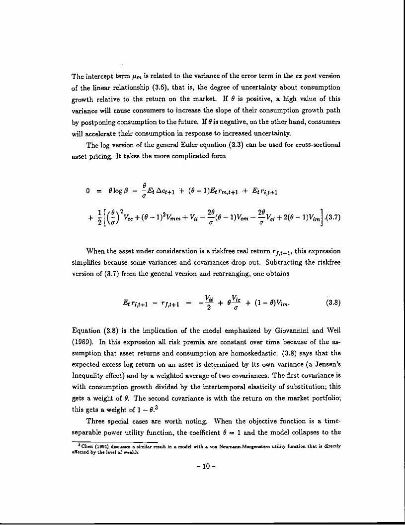
The intercept term Pm is related to the variance of the error term in the z post version

of the linear relationship (3.6), that is, the degree of uncertainty about consumptiongrowth relative to the return on the market. If 9 is positive, a high value of thisvariance will cause consumers to increase the slope of their consumption growth path

by postponing consumption to the future. If 9 is negative, on the other hand, consumers

will accelerate their consumption in response to increased uncertainty.The log version of the general Euler equation (3.3) can be used for cross-sectional

asset pricing. It takes the more complicated form

o = Olog/3 — .!E Act+i 4- (9— I)Etrm,g+i -f Etr1,j÷1

+ + (9 1)2 1/mm + Vu — — 1)V,,, — + 2(9 —flVim]

.(3.7)

When the asset under consideration is a riskfree real return this expression

simplifies because some variances and covariances drop out. Subtracting the riskfree

version of (3.7) from the general version and rearranging, one obtains

VjjE r,t+i — Df,g+i =2

+ 9-;- + (1 — $)Vim. (3.8)

Equation (3.8) is the implication of the model emphasized by Giovannini and Weil(1989). In this expression all risk premia are constant over time because of the as-sumption that asset returns and consumption are homoskedastic. (3.8) says that theexpected excess log return on an asset is determined by its own variance (a Jensen'sInequality effect) and by a weighted average of two covariances. The first covariance is

with consumption growth divided by the intertemporal elasticity of substitution; thisgets a weight of 9. The second covariance is with the return on the market portfolio;

this gets a weight of 1 — 9•3

Three special cases are worth noting. When the objective function is a time-separable power utility function, the coefficient 9 = 1 and the model collapses to the

3Ches, (1991) discussa & similar result in a model with a von Neiunann-Morgenstem utility (unction that i. directlyaffected by the level of wealth.

— 10 —

loglinear consumption CAPM of Hansen and Singleton (1983). When the coefficient ofrelative risk aversion = 1, 8 = 0 and a logarithmic version of the static CAPM pricing

formula holds. Most important for the present paper, as the elasticity of intertemporal

substitution a approaches one the coefficient 9 goes to infinity. At the same timethe variability of the consumption-wealth ratio decreases so that the covariance Vj

approaches Vim. It does not follow, however, that the risk premium is determined only

by 14m in this case. Giovannini and Weil (1989) show that the convergence rates aresuch that asset pricing is not myopic when a = 1 unless also y = 1 (the log utilitycase). In the next section I give an exact expression for the risk premium in the a =1

case.

3.2. Substituting Out Consumption

The loglinear Euler equations derived above can now be combined with the ap-

proximate loglinear budget constraint of section 2. Substituting (3.6) into (2.9), oneobtains

cg—wj = (1—a)Ej Erm+j + p(k—pm)(3.9)

The log consumption-wealth ratio is a constant, plus (1—a) times the discounted value

of expected future returns on invested wealth. If a is less than one, the consumer isreluctant to substitute intertemporally and the income effect of higher returns dom-inates the substitution effect, raising today's consumption relative to wealth. If a isgreater than one, the substitution effect dominates and the consumption-wealth ratiofalls when expected returns rise. Thus equation (3.9) extends to a dynamic context the

classic comparative statics results of Samuelson (1969) and Merton (1969).

Note that the coefficient of relative risk aversion 1 does not appear in (3.9) except

indirectly through the parameter of linearization p. Kandel and Starnbaugh (1991) haveused a numerical solution method to show that a rather than is the main determinant

of the variability of expected market returns in a model with exogenous consumption

and endogenous returns. Equation (3.9) provides a simple way to understand their

finding.

— 11 —

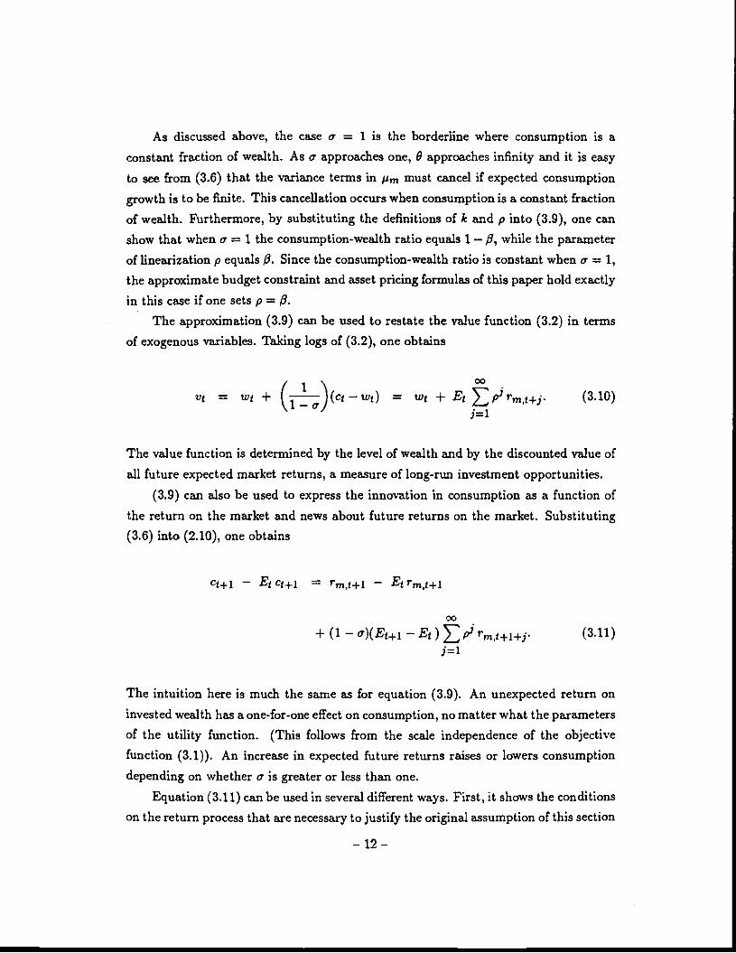
As discussed above, the case a = 1 is the borderline where consumption is aconstant fraction of wealth. As a approaches one, 9 approaches infinity and it is easy

to see from (3.6) that the variance terms in ji must cancel if expected consumptiongrowth is to be finite. This cancellation occurs when consumption is a constant fraction

of wealth. F\rthermore, by substituting the definitions of Ic and p into (3.9), one can

show that when a = 1 the consumption-wealth ratio equals 1 — , while the parameterof linearization p equals (3. Since the consumption-wealth ratio is constant when a =1,

the approximate budget constraint and asset pricing formulas of this paper hold exactly

in this case if one sets p =

The approximation (3.9) can be used to restate the value function (3.2) in terms

of exogenous variables. Taking logs of (3.2), one obtains

vi = wi + (11 ) twz) = wi + Etp5r15. (3.10)

The value function is determined by the level of wealth and by the discounted value of

all future expected market returns, a measure of long-run investment opportunities.

(3.9) can also be used to express the innovation in consumption as a function of

the return on the market and news about future returns on the market. Substituting(3.6) into (2.10), one obtains

— .E cjj = — E1 rmg+1

+ (1 —a)(Ej1 —Ei)rm,t÷i+j. (3.11)

The intuition here is much the same as for equation (3.9). An unexpected return on

invested wealth has a one-for-one effect on consumption, no matter what the parameters

of the utility function. (This follows from the scale independence of the objectivefunction (3.1)). An increase in expected future returns raises or lowers consumption

depending on whether a is greater or less than one.

Equation (3.11) can be used in several different ways. First, it shows the conditions

on the return process that are necessary to justify the original assumption of this section

— 12 —

that consumption growth and asset returns are jointly lognormai. To a first approxima-

tion, consumption growth will be lognormal if the return on the market and revisions

•of expectations about future returns are jointly lognorinal; thus the assumption of joint

lognormality of consumption growth and asset returns can be approximately consistent

with equilibrium.

Second, the equation shows when consumption will be smoother than the returnon the market. There is some evidence of "mean reversion" in aggregate stock returns,

that is, a negative correlation between current returns and revisions in expectations offuture returns (Faxna and French 1988a, Poterba and Summers 1988). According to

(3.11), mean reversion reduces the variability of consumption growth if the elasticityof intertemporal substitution a is less than one. Mean reversion amplifies the volatility

of consumption growth, however, if a is greater than one.

To understand this more clearly, it may be helpful to consider a simple examplein which the market return follows a univariate stochastic process: rmj+1 = A(L)ct+i.Here the polynomial in the lag operator A(L) 1 + a1L + a2L2 + ..., where thecoefficients a are the moving average coefficients of the market return process. Simi-larly, one can define A(p) E I + ap + ap2 +..., the infinite sum of moving average

coefficients discounted at rate p. Since p is close to one A(p) is approximately the

sum of the moving average coefficients, a measure of the impact of today's return in-

novation on long-run future weaith. In this special case (3.11) can be rewritten as— Ejc(+i = t--i +(1 — c)(A(p) — 1)t÷i = cej+l +(1 —c)A(p)et+i. The innovation

in consumption is a weighted combination, with weights a and 1 —a, of the currentmarket return innovation €j4 and the discounted long-run impact of the return inno-vation A(p)et+i. Mean reversion in the market return makes A(p) C 1, which reduces

the variability in consumption ifa .c 1.

Third, equation (3.11) can be used to clarify the interpretation of the intercept

coefficient Pm in the equation relating consumption growth and the expected returnon the market. Substituting (3.11) into (3.6), Pm can be written as

Pm = clogP + ()(i — c)2 (f)va.rt [E1+1 — Etrm,÷l+j]

= clog$ + ()(1 — a)2 (!) Varg Vjj. (3.12)

— 13 —

The summation in (3.12) runs from zero to infinity, since the uncertainty that affects

Pm includes both the variance of this period's market return and the variance of news

about future market returns. The second equality in (3.12) follows from the solutionfor the value function (3.10). (3.12) shows that the conditional variance of expectedlong-run investment opportunities (equivalently, the conditional variance of the value

function) is the correct measure of risk in this model. As discussed above, the sign of

B determines whether consumers will postpone or accelerate consumption in response

to this risk.Finally, equation (3.11) implies that the covariance of any asset return with con-

sumption growth can be rewritten in terms of covariances with the return on the market

and revisions in expectations of future returns on the market.4 The covariance satisfies

Coy2 (r1,j+i, Acj+i) = V + (1 — c)Vih, (3.13)

where

Coy2 (ri,t+i, (Et+i — Et) E p1 rmt+i+4. (3.14)j= I

11th is defined to be the covariance of the return on asset i with good news about future

returns on the market, i.e. upward revisions in expected future returns.5

Substituting (3.13) into (3.8) and using the definition of Bin terms of the underlying

parameters a and , I obtain a cross-sectional asset pricing formula that makes noreference to consumption:

Et r12÷1 — rf,g+1 = + 7Vm + ( — flV. (3.15)

Equation (3.15) has several striking features. First, assets can be priced without

Equally1 (3.11) could be used to rewrite the covariance with the market in ten,.. of covaxiances with consumption andrevisions in expectation, of future investment opportunities. The contribution of (3.11) is to show that oniy two of thesethree conrianc need be measured accurately in order to have a testable asset pricing theory.

5The notation V, is chosen to accord with Campbell (iSOla). It recall, the standard tenninolcgy of 'hedge portfolioC(e.g. Ingersoll 1987).

— 14 —

direct reference to their covariance with consumption growth, using instead their co-variances with the return on invested wealth and with news about future returns on

invested wealth. This is a discrete-time analogue of Merton's (1973) continuous-time

model in which assets are priced using their covariances with certain "hedge portfolios"

that index changes in the investment opportunity set.

Second, the only parameter of the utility function that enters (3.15) is the coeffi-cient of relative risk aversion y. The elasticity of intertemporal substitution c does not

appear once consumption has been substituted out of the model. This is in strikingcontrast with the important role played by a in the consumption-based Euler equation

(3.8). Intuitively, this result comes from the fact that a plays two roles in the theory.A low value of a reduces anticipated fluctuations in consumption (equation (3.6)), but

it also increases the risk premium required to compensate for any contribution to these

fluctuations (equation (3.8)). These offsetting effects lead a to cancel out of the asset-

based pricing equation (3.15). Kocherlakota (1990) and Svensson (1989) have alreadyshown that a is irrelevant for asset pricing when asset returns are independently and

identically distributed over time. This is not surprising, since with i.i.d. returns there is

no interesting role for intertemporal substitution in consumption. The present result isapproximate but is much stronger, since it holds in a world with changing conditionalmean asset returns.

Third, equation (3.15) expresses the risk premium (net of the Jensen's inequalityeffect) as a weighted sum of two terms. The first term is the asset's covariance with the

market portfolio; the weight on this term is the coefficient of relative risk aversion y.The second term is the asset's covariance with news about future returns on the market;

this receives a weight of 7—1. When 'y is less than one, assets that do well when there

is good news about future returns on the market have lower mean returns, but when

is greater than one, such assets have higher mean returns. The intuitive explanation is

that such assets are desirable because they enable the consumer to profit from improved

investment opportunities, but undesirable because they reduce the consumer's ability

to hedge against a deterioration in investment opportunities. When C I the former

effect dominates, and consumers are willing to accept a lower return in order to holdassets that pay off when wealth is most productive. When > i the latter effect

dominates, and consumers require a higher return to hold such assets.

There are several possible circumstances under which assets can be priced using

only their covariances with the return on the market portfolio, as in the logarithmic

— 15 —

version of the static CAPM. These cases have been discussed in the literature on in-

tertemporal asset pricing, but equation (3.15) makes it particularly easy to understandthem. First, if the coefficient of relative risk aversion 7 = 1, then the opposing effectsof covariance with investment opportunities cancel out so that only covariance with the

market return is relevant for asset pricing. Giovannini and Weil (1989) emphasize this

result, and it has been long understood for the special case of log utility, where not only

= 1, but also a = 1. Second, if the investment opportunity set is constant, then Vhis zero for all assets so again assets can be priced using only their covariances with the

market return. Farna (1970) and Merton (2969, 1971) stress this result. Third, if thereturn on the market follows a univariate stochastic process, then news about futurereturns is perfectly correlated with the current return. Using the lag operator notation

introduced above, in this case V111, = (A(p)1)Vjm for all assets i, and the risk premium

(ignoring the Jensen's inequality term) is [-y + (y — 1)(A(p) — 1)]Vim. Giovannini and

Weil (1989) and Merton (1990, Chapter 16) present results of this type in discrete timeand continuous time respectively.

One obvious application of the formula (3.15) is to the equity premium, the risk

premium on the market itself. When the market return is serially uncorrelated, the

equity premium net of the Jensen's Inequality term is just 7Vmm, and the coefficient of

relative risk aversion can be estimated in the manner of Friend and Blume (1975) by

taking the ratio of the equity premium to the variance of the market return. However

this procedure can be seriously misleading if the market return is serially correlated.

With a univariate market return process, for example, the equity premium net of theJensen's Inequality term is fy + (y— 1)(A(p) —1)]Vmm. Mean reversion in stock returns

(the case A(p) c 1) reduces the equity premium when 'y > 1 but increases it whenc 1. The Friend and Blume estimate of risk aversion will be off by (7— 1)(.4(p) —1).

This error can be substantial, particularly if is very large as suggested by Kandel and

Stambaugh (1991) among others. Black (1990) also emphasizes that mean reversioncan affect the relation between short-run market volatility and the equity premium.

3.3. The Term Structure of Real Interest Rates

Real bonds, which make fixed payments of consumption goods, play a special role

in asset pricing theory because they have no payoff uncertainty. The only uncertainty intheir return comes from changes in the real interest rates used to discount their payoffs.

— 16 —

In this section I show that in a lognormal homoskedastic model, the unexpected return

on a real consol bond is approximately equal to minus the news about future returns on

invested wealth. This means that the covariance with good news about future returns

can also be written as minus the covariance with the return on a real consol.

Let P6 denote the log price at time i of a real consol bond paying 1 unit of the

consumption good each period, with no maturity date. The log return on this bond is

E log(1 + exp(p6 ÷i)) — Po. (3.16)

Linearizing this expression with a first-order Taylor expansion in the manner of section2, one obtains the approximation

!c, + PbPot+1 — (3.17)

where Pb is the reciprocal of the average gross, simple return on the consol: p = 1/R6.

This implies that Pbi is determined by the discounted value of expected futurereturns on the bond, or equivalently by the discounted value of expected future returns

on invested wealth (in the homoskedastic model these are the same, up to a constant

risk premium):

Pbi = Ej Eprmj+j + 1c, (3.18)

for some constant P. Substituting (3.18) back into (3.17), one obtains

Tb,t+1— = —(Ej+i — E ) rmj+1+j. (3.19)

In general Pb does not equal the parameter of linearization for the intertemporalbudget constraint, p. However the difference is likely to be small, and it will have

— 17—

little effect on a discounted value like the right hand side of (3.19) if news about future

returns on the market dies out fairly rapidly. Thus

Cov(r1j+i,r&÷i) V16 (3.20)

and the asset pricing equation (3.15) can be rewritten as

— rf,ji = + 7V1m + (1 7)V1a (3.21)

Equation (3.21) says that the expected log return on any asset is determined by itsown variance, and by a weighted average of its covariances with the market portfolioand with a real consol bond. The weights on the market and the consol are and 1 —y

respectively, where as before y is the coefficient of relative risk aversion.

Equation (3.21) is reminiscent of the formula in Merton (1973) that expresses the

expected excess return on any asset as a linear function of its covariances with themarket and with the return on an asset perfectly correlated with changes in short-term interest rates (loosely, a long-term bond).6 However the present model differsfrom Merton's in t important respects. First, Merton's result depends on the as-sumption that all changes in investment opportunities are summarized by the changein a single state variable, the instantaneous interest rate. Here, the short-term inter-est rate summarizes the current investment opportunity set (because all asset returns

move in parallel in the homoskedastic model), but it does not summarize all changes

in investment opportunities (because there can be many sources of news about future

returns). Another way to see the difference is to note that in Merton's model long-term

bond returns and changes in short-term rates are perfectly correlated instantaneously,

whereas this need not be the case in the present model.7 Second, Merton's model gives

the prices of the two sources of risk only in terms of the derivatives of the consumer's

value function, which are endogenous to the model. Here, the risk prices are explicitly

determined by the primitive parameters of the consumer's utility function.

6Thi. is equation (32) of Merton (1973), reprinted as equation (15.32) in Merton (1993). Bossae,t. and Green (1989),Breeden (1986). and Rubinatein (1981) also emphashe the importance of real bonds in asset pricing.

1In another respect, howeva, Merton's model is more gena'al because it allow. variance, to depend on the interestrate. In the next section I allow for changing variance, in the present framework.

— 18 —

3.4. A Vector Autoregressive Factor Pricing Model

The results of the previous section would be useful for empirical work if real consol

returns were observable. Unfortunately such assets do not exist; the closest equivalent

may be finite-maturity index bonds in the United Kingdom, and even these have been

actively traded only in recent years. Another approach is needed to derive testableimplications of the basic asset pricing equation (3.15).

Here I adapt the vector autoregressive approach of Campbell (1991a).8 I assumethat the return on the market can be written as the first element of a K-element state

vector zj. The other elements are variables that are known to the market by the end

of period t + 1, and are relevant for forecasting future returns on the market. I assumethat the vector i4 follows a first-order vector autoregression (VAR):

= Az + f+1- (3.22)

The assumption that the VAR is first-order is not restrictive, since a higher-order VAR

can always be stacked into first-order (companion) form in the manner discussed byCampbell and Shiller (lOSSa). The matrix A is known as the companion matrix of theVAR.9

Next I define a K-element vector ci, whose first element is one and whose other

elements are all zero. This vector picks out the real stock return tm,g+j from thevector zj+1: rm,g+1 = el1zj÷i, and rm+1 —Et rm,j+1 = el'ej+l. The first-order VARgenerates simple multi-period forecasts of future returns:

Eg rmf+1+j = ei'A'4'zt. (3.23)

It follows that the discounted sum of revisions in forecast returns can be written as

tCampbell uses this aprroadi to decompose the overall market return into news about dividends and news about futuremarket return. In the present homoskedanic context the latter component is just the return on a real consd, as discussedabove. Equation (3.15) says that the dividend news component of the market return has risk price i while the returnnews component has risk price I —

As is well known, VAR systems can be normalized in different ways. For exampie, the variables in the state vector canbe orthogonslized so that the nzianc.conriance matrix of the enor vedor c is diagonal. The results given below holdfor any observationaily equivalent nonnalatIon of the VAR system.

— 19 —

(Ej+i =

= el'pA(I —

= :+i, (3.24)

where A' is defined to equal el'pA(I — a nonlinear function of the VAR cod-

ficients. The elements of the vector A measure the importance of each state variable

in forecasting future returns on the market. If a particular element Ak is large andpositive, then a shock to variable k is an important piece of good news about future

investment opportunities.I now define

E Covg (r;,g+i, k,i+1)' (3.25)

where ks+1 is the k'th element of eg.. Since the first element of the state vector isthe return on the market, V = v1,. Then equations (3.24), (3.25), and (3.15) implythat

Et rI,+j — = — + -1V11 + (-y— 1) A114k, (3.26)

where Ak is the k'th element of A. This is a standard K-factor asset pricing model,

and its general form could be derived in any number of ways: perhaps most straight-

forwardly by using the Arbitrage Pricing Theory of Ross (1976).The contribution of the intertemporal optimization problem is a set of restrictions

on the risk prices of the factors. The first factor (the return on the market) has a riskprice of 'y + (-y— 1)Ai. A positive value of A1 means that the return on the market is

positively correlated with revisions in expected future returns, while a negative value

— 20 —

of A1 means that the market return is "mean reverting". These serial correlationproperties of the market return affect the risk price of the market factor; if the market

is mean reverting, for example, its risk price is reduced if y is greater than one.

The other factors in this model have risk prices of (y — 1)Ak. Factors here arevariables that help to forecast the return on the market, and their risk prices areproportional to their forecasting importance as measured by the elements of the vectorA. If a particular variable has a positive value of Ak, this means that innovations inthat variable are associated with good news about future investment opportunities.

Following the analysis in section 3.2, such a variable will have a negative risk price ifthe coefficient of relative risk aversion i' is less than one, and a positive risk price if the

coefficient of relative risk aversion is greater than one.

Thus the intertemporal model suggests that priced factors should be found not by

running a factor analysis on the covariance matrix of returns (Roll and Ross 1980), nor

by selecting important macroeconomic variables (Chen, Roll, and Ross 1986). Instead,variables that have been shown to forecast stock market returns should be used incross-sectional asset pricing studies. Recent empirical work suggests that dividend

yields, interest rates and other financial variables are likely to be important (Campbell

1987,1991a, Campbell and Shiller 1988a,b, Fama and Schwert 1977, Fama and Ftench

1988b,1989, Keim and Starnbaugh 1986).

— 21 —

4. Intertemporal Asset Pricing with Changing Variances

In this section I relax the unrealistic assumption of the previous section that allvariances and cova.riances of log asset returns and consumption are constant through

time. Relaxing this assumption has no effect on the log-linearization of the budgetconstraint in section 2 or the formulation of the intertemporal optimization problem in

section 3.1. What it does do is change the log form of the Euler equations for this prob-

lem. If asset returns and consumption are jointly lognormal, but heteroskedastic rather

than homoskedastic, equations (3.5) through (3.8) hold with time t subscripts on thevariances and covariances; constants of the form become variables of the form V,,1.

These modified log Euler equations also hold as second-order Taylor appraimations ifasset returns and consumption are not lognormal.

The more general form of equation (3.6) is

E Act÷i = p,nj + aEj rm÷1,

= clog$ + [ + OcVmmt —2evcmi]

= clog$ + a)Vart[ct÷1 (4.1)

The intercept Pmi, which was previously constant, now changes over time with thevariance of consumption growth relative to the market return. This means that when

(4.1) is substituted into the approximate loglinear budget constraint (2.9), extra terms

appear in the formulas for the log consumption-wealth ratio and the innovation in log

consumption. Equation (3.11) becomes

— = rm,t÷1 —

+ (1—c)(Ej+i —Ec)rm.i+i+j

— (Eg÷i_-Et)Ep)p,+. (4.2)

The new term in equation (4.2) reflects the influence of changing risk on saving. Thevariable Pm is proportional to the conditional variance of consumption growth less atimes the return on invested wealth. As this changes, consumers may be induced to

accelerate or postpone consumption. The difficulty is that equation (4.2), unlike thehomoskedastic equivalent (3.11), still makes reference to consumption growth on theright hand side through the variable /1m1 which is a function of the second moments of

consumption. Thus equation (4.2) cannot be used to substitute consumption growthout of the intertemporal asset pricing model without further assumptions.

There are, however, several special cases in which consumption can be substituted

out of the model with changing variances. First, if the coefficient of relative risk aversion= 1, then 0 = 0 and Pin remains constant even in the heteroskedastic case. Thus

when 'y = I a logarithmic version of the static CAPM holds with changing conditional

variances. Second, if the elasticity of intertempora2 substitution a = 1, 0 is infinite

and the conditional variance in (4.1) must be zero. In this case the intertemporalasset pricing formula (3.15) continues to hold with time subscripts on the conditional

variances. Presumably this formula is a good approximation if a is not too far fromone or if conditional variances are not highly variable or persistent. Third, the asset

pricing formula (3.15) describes any asset returns that are uncorrelated with revisions

in expectations of future intercepts Pmt+j• Restoy (1991), building on the analysisof this paper, has shown that (3.15) describes the equity premium if the variance ofmarket returns follows a GARCH process that is uncorrelated with the return on themarket.

A final special case assumes, in the spirit of Cox, Ingersoll, and Ross (1985), that

the intercept Pint is a linear function of the expected return on the market. Supposethat

Pm,t = /10 + Etrt+i (4.3)

for some coefficient Then the innovation in consumption can be rewritten as

"This condition is slightly probkmatic in • discrete time mode!, because strictly speaking itis inconsistent with thenormality of conditional expected returns on the market and the positivity of the variances defimng /m \VlietI. this ita serious proWem wili depend on the parameter values of the model.

— 23 —

— Egc+, = rmf+1 —

+ (1—c — — Ej Dmt+l+j. (4.4)

It follows that the covariance of any asset return with consumption growth can be

written as

Coy1 (r1,j+i, c1+i) = — (1 — — V')"in,t, (4.5)

and the expected excess return on any asset is given by

E1 rit+l — rj,11 = + 7m,1 + [(71) — Vih,t. (4.6)

This formula for the risk premium is the same as before, with the addition of a terminvolving the sensitivity of the consumption intercept to the expected return on the

market, b. This term may be positive or negative in general, and it is interpreted as

follows. A 1% increase in the expected return on the market lowers consumption by

% through the precautionary saving channel. The market price of consumption riskis 9/a, so the market price of investment opportunity set risk includes a term —9'/a.

It is important to find conditions on the exogenous process for asset returns that

justify the assumption on Pint (4.3). One can show that Pint will satisfy (4.3) if the

variances and covariance of the return on the market and news about future returns onthe market are linear functions of the expected return on the market. In other words,

if for {r,y} = {rn,h} we have that

= + VJEtr,t+i, (4.7)

then (4.3) is satisfied." This assumption on returns is a discrete-time analogue of the

assumption used in Cox, Ingersoll, and Ross (1985)." However some v.Ju of the slope coefficient, in (4.7) maygive a compicx tether than real .oluticn for .

— 24 —

In this model the variance-covariance matrix of the return on the market and news

about future returns on the market changes with one underlying variable, the expected

return on the market. This means that the expected excess return on the market, as

given by equation (4.6) for asset I = in, can be written as a linear function of theconditional variance of the return on the market. Substituting (4.7) into (4.6) for asset= in, one obtains

Eirm+i —rp÷i = o + PiVmm.i

Pa = ____

1 /th (4.8)

This result sheds new light on the large empirical literature that estimates a linearrelation between the conditional mean and variance of the return on the aggregate

stock market (for example Bollerslev, Engle, and Wooldridge 1988, French, Schwert,and Stambaugh 1987, and Merton 1980). It is sometimes argued that linearity will hold

in a fully specified intertemporal asset pricing model only if agents have log utility. Themodel of this section provides a counter-example to this claim. It is important to note,however, that the market price of conditional volatility, given by the coefficient P1 inequation (4.8), does not generally equal the coefficient of relative risk aversion 7.

— 25 —

5. How Accurate is the Log-Linear Approximation?

Earlier sections of the paper. have stated some strikingly simple results aboutthe determination of expected asset returns. These results are based on a log-linear

approximation to the intertemporal budget constraint that will be accurate when thelog consumption-wealth ratio is "not too" variable. In this section I try to characterize

more precisely the circumstances under which the approximation works well. To do

this, I assume a specific market return process and consider alternative parametervalues for the representative consumer's objective function. For each set of parameter

values I calculate optimal consumption functions numerically and compare them withthe approximate analytical solutions derived above.

To reduce the complexity of the problem, I first specialize the model of section

3 to a simple example discussed in Campbell (1991a). In this example, the expectedreturn on the market portfolio follows a univariate AR(1) process with coefficient ,while the realized return is the expected. return plus a white noise error. This shouldnot be confused with the special case discussed in previous sections in which the market

return itself is a univariate process. The model considered here is

= E1 rm,g+1 + E1,t+1

Et+i tm,j+2 = t/E1 rm,j+1 + 2t+l• (5.1)

The free parameters of this model are the coefficient and the second moments V11, 1(12,

and V22.

The next step is to pick reasonable values for these parameters. Campbell (1991a)

estimates persistence measures for expected returns using CRSP monthly data on value-

weighted U.S. stock returns over the period 1927-1988. The persistence measures are

estimated using a VAR system of the type discussed in section 3.4, rather than the sim-

ple AR(1) model (5.1). However it is straightforward to calculate the AR(1) parameter

that would correspond to any VAR persistence measure. Campbell's estimates imply= 0.79 over the full 1927-1988 sample period, and a similar value of = 0.83 in the

postwar 1952-1988 sample period. Thus =0.8 is a realistic benchmark value to usein the AR(1) model. This value of implies a haiflife for expected return shocks of

— 26 —

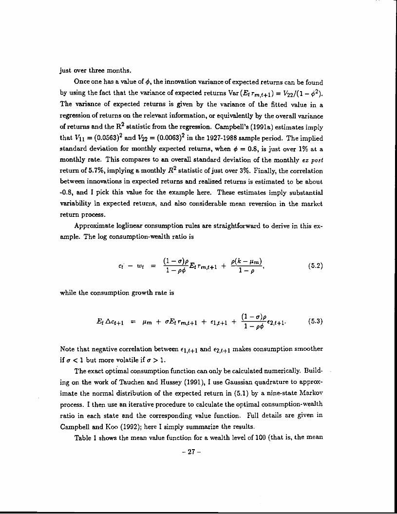
just over three months.

Once one has a value of 4i, the innovation variance of expected returns can be found

by. using the fact that the variance of expected returns Var(Ej rm,j+1) =11221(1—

The variance of expected returns is given by the variance of the fitted value in a

regression of returns on the relevant information, or equivalently by the overall variance

of returns and the R2 statistic from the regression. Campbell's (1991a) estimates imply

that Vjj = (0.0563)2 and V22 = (0.0063)2 in the 1927-1988 sample period. The impliedstandard deviation for monthly expected returns, when = 0.8, is just over 1% at amonthly rate. This compares to an overall standard deviation of the monthly ez postreturn of 5.7%, implying a monthly J?2 statistic of just over 3%. Finally, the correlation

between innovations in expected returns and realized returns is estimated to be about-0.8, and I pick this value for the example here. These estimates imply substantial

variability in expected returns, and also considerable mean reversion in the market

return process.Approximate loglinear consumption rules are straightforward to derive in this ex-

ample. The log consumption-wealth ratio is

(1—c)p p(k—.um)ci — =1— Etrm,t+i + 1— (5.2)

while the consumption growth rate is

= Pm + cEtrt+i + 61,1+1 + (5.3)

Note that negative correlation between i,i+1 and 2t+1 makes consumption smoother

if o- c 1 but more volatile if a> 1.

The exact optimal consumption function can only be calculated numerically. Build-

ing on the work of Tauchen and Hussey (1991), I use Gaussian quadrature to approx-

imate the normal distribution of the expected return in (5.1) by a nine-state Markov

process. r then use an iterative procedure to calculate the optimal consumption-wealth

ratio in each state and the corresponding value function. Full details are given inCampbell and Koo (1992); here I simply summarize the results.

Table 1 shows the mean value function for a wealth level of 100 (that is, the mean

— 27 —

value function as a percentage of wealth), calculated numerically for a grid of six values

of a and six values of y. a is set equal to 0.05, 0.50, 1.00, 2.00, 3.00, and 4.00, while

is 0.00, 0.50, 1.00, 2.00, 3.00, and 4.00. The smallest value of a is 0.05 rather than 0.00

because the program encounters some numerical difficulties when a is extremely small.

All the results reported assume that the mean market return is 6.5% at an annual rate

and that the discount factor /3 is the twelfth root of 0.94, giving the monthly equivalent

of a 6% annual discount rate.Table 1 also shows the percentage losses in the mean objective function that result

from using the loglinear consumption rule (3.9). Since the objective function has been

normalized to be linear in wealth, these losses have the same units as reductions inwealth. The first number in parentheses is the percentage utility loss when p is obtained

from (2.5) with the true optimal value of the mean log consumption-wealth ratio. The

second number in parentheses is the percentage utility loss when p is set equal to /3,

its value for the a = 1 case. The first procedure gives a more accurate approximation,

but it requires knowledge of the true mean log consumption-wealth ratio. The second

procedure is less accurate but more easily implementable in practice.

As one would expect, the utility losses from using loglinear consumption rulesincrease as a moves further from unity. The losses are zero when a = 1, for thenthe approximations are exact. When a = 0.5 or 2.00, the approximate consumptionfunctions cost less than 0.01% of wealth unless 7 is at its highest value of 4.00. Whena = 0.05, 3.00, or 4.00, the approximate consumption function with the correct p still

costs no more than 0.01% of wealth, but the approximate consumption function setting

p = /3 is noticeably less accurate. As an extreme case, when both a and 7 are at their

maximum values of 4.00, this approximation costs 1.2% of wealth.

Table 2 shows mean optimal consumption as a percentage of wealth. Since j3and the expected return process are fixed, the mean consumption-wealth ratio variesconsiderably as the parameters and a vary. The smallest value in the table is 0.237%

(2.84% at an annual rate) when a = 4.00 and = 0.00. The largest value is 1.05%

(12.6% at an annual rate) when a = 4.00 and 1 = 4.00. The table also reportsthe differences between the exact and approximate mean consumption-wealth ratios,

expressed as percentages of the exact mean consumption-wealth ratio. These differences

are again zero when a = 1, but they increase quite rapidly as a moves away from one.

When the approximation uses the true p, the error is 0.05% to 0.25% of the exact mean

consumption-wealth ratio when a = 0.05 or 2.00, increasing to almost 1.5% of the exact

— 28 —

mean consumption-wealth ratio when a = 4.00. When the approximation uses p = /3,

the errors can be many times larger.

If one is interested in the dynamic behavior of consumption and its implications for

asset pricing, errors in the mean consumption-wealth ratio are relatively unimportant.

What is important is to approximate accurately the variation of the consumption-wealth ratio and the consumption growth rate around their means. Table 3 givesthe standard deviation of the optimal log consumption-wealth ratio, along with thepercentage errors of the two approximations. The log ratio is used because this isapproximately normally distributed. The table shows that as a approaches one, theapproximation error for the log standard deviation goes to zero at almost the same rateas the log standard deviation itself. Thus in percentage terms the approximation error

is almost constant and small at about 0.75% of the true standard deviation. Table 4

reports the standard deviation of the optimal log consumption growth rate, again withthe percentage errors of the two approximations. The consumption-smoothing effectof mean reversion when a is low is clearly visible in this table. The approximations

tend to understate the variability of log consumption growth when a is low and tooverstate the variability when a is high. However the errors are quite small, nevermuch above 0.5% of the true standard deviation when the correct value of p is used.

The approximation setting p = /3 should be used more cautiously, as its maximum error

is four times greater than the the approximation error using the true p.These results are encouraging for two reasons. First, they are obtained using a

model in which the expected return on the market is highly variable. Less extreme

variability in the expected return process would increase approximation accuracy byreducing the variability of the optimal consumption-wealth ratio. Second, a numberof authors (Campbell and Mankiw 1989, Giovannini and Weil 1989, Hall 1988, Kandel

and Stambaugh 1991) have argued from direct evidence on consumption and asset price

behavior that a is more likely to be very small than very large. Tables 3 and 4 show that

a loglinear approximation to the interternporal budget constraint is workably accurate

when a is close to zero, even if the true value of p is unknown.

— 29 —

6. Conclusions.

In this paper I have argued that intertemporal asset pricing theory has become

unnecessarily tangled in complications caused by the nonlinearity of the intertemporalbudget constraint. I have proposed a log-linear approximation to the constraint as away to cut this Gordian knot. In a simple example calibrated to U.S. stock return data,

the approximation seems to be workably accurate when the elasticity of intertemporal

substitution is less than about 3.I assume that asset returns and news about future returns are jointly lognormal

and homoskedastic, and that there is a representative agent who maximizes the objec-

tive function proposed by Epstein and Zin (1989, 1990) and Weil (1987). This objective

function has many of the appealing features of the time-separable power utility func-

tion, but it separates the elasticity of intertemporal substitution a from the coefficientof relative risk aversion rather than forcing these parameters to be reciprocals ofone another as in the power utility case. The log-linear approximation to the bud-get constraint then yields some simple propositions about consumption behavior and

intertemporal asset pricing.

1. The log consumption-wealth ratio equals a constant, plus (1 —a) times the dis-counted value of all future expected returns on invested wealth. The innovation

to log consumption equals the innovation to the log return on the market, plus(1— a) times the revision in the discounted value of future market returns. As one

would expect, the coefficient a rather than governs the response of consumptionto changing expected asset returns.

2. The expected excess log return on any asset over the riskfree return is the sum of

three terms. The first term is minus one half the own variance of the log assetreturn, a Jensen's Inequality effect. The second term is y times the covariance ofthe asset return with the return on the market, as in a logarithmic version of the

static CAPM. The third term is 1—'y times the covariance of the asset return with

news about future returns on the market. As one would expect, the coefficient 7rather than a determines the size and sign of asset risk premia.

3. In the homoskedastic model, the log return on a real consol bond is approximately

equal to minus the news about future returns on the market. Thus the expectedexcess return on any asset, net of the Jensen's Inequality effect, can also be written

as a weighted average of the asset's covariance with the market and with the consol.

—30—

The weights are 7 and 1 — 7 respectively.

4. If the return on the market can be written as one element of a state vector that

follows a homoskedastic vector autoregression (VAR), then the intertemporal theory

delivers a set of restrictions on the risk prices of a factor asset pricing model. The

factors are variables that are relevant for forecasting the market and hence enterthe VAR state vector. Their risk prices are proportional to their importance inforecasting the discounted value of future returns on the market.

5. The results above can be generalized to allow a restricted form of heteroskedasticity

in asset returns. If the conditional variance-covariance matrix of the return on themarket and news about future returns on the market is linear in the expected return

on the market, then the asset pricing model goes through as before, except that theprice of covariance with news about future returns is no longer equal to 1— 'y. With

this form of heteroskedasticity, the expected excess return on the market is linear

in the conditional variance of the return on the market, as commonly assumed in

empirical work. The homoskedastic results also generalize straightforwardly if a or

'y are sufficiently close to one.

These results have pedagogic value as a simple way to understand the vast andcomplicated literature on intertemporal asset pricing. They also raise the hope that

this subject can be brought into a closer relationship with the equally large body ofwork on cross-sectional factor asset pricing models. An important topic for futureresearch will be to test the restrictions placed by the approximate intertemporal model

on cross-sectional factor risk prices.

The main difficulty in conducting such a test is that, as emphasized by Roll (1977),

the return on the market portfolio is imperfectly measured. If neither consumption

data nor market return data are adequate, then it may be necessary to develop amore explicit general equilibrium model in which macroeconomic variables help toidentify the returns on physical and human capital. The loglinear approximation of this

paper has already been used to solve real business cycle models by Campbell (1991b),

Christiano (1088), King, Plosser, and Rebelo (1987) and others, and the application of

macroeconomic models to asset pricing promises to be another active area of research,

—31—

Bibliography

Black, Fischer, 1990, "Mean Reversion and Consumption Smoothing", Review of Fl-nancial Studies 3, 107—114.

Bollerslev, Tim, Robert F. Engle, and Jeffrey Wooldridge, 1988, "A Capital AssetPricing Model with Time Varying Covariances", Journal of Political Economy 96,116—131.

Bossaerts, Peter and Richard C. Green, 1989, "A General Equilibrium Model of Chang-ing Risk Premia: Theory and Tests", Review of Financial Studies 2, 467—493.

Breeden, Douglas, 1979, "An Intertemporal Asset Pricing Model with Stochastic Con-sumption and Investment", Journal of Financial Economics 7, 265—296.

Breeden, Douglas, 1986, "Consumption, Production, Inflation, and Interest Rates: ASynthesis", Journal of Financial Economics 16, 3—39.

Breeden, Douglas T., Michael ft. Gibbons, and Robert H. Litzenberger, 1989, "Empir-ical Tests of the Consumption-Oriented CAPM", Journal of Finance 44, 231—262.

Brown, David P. and Michael ft. Gibbons, 1985, "A Simple Econometric Approach forUtility-Based Asset Pricing Models", Journal of Finance 40, 359—381.

Campbell, John Y., 1987, "Stock Returns and the Term Structure", Journal of Finan-cial Economics 18, 373—399.

Campbell, John Y., 1991a, "A Variance Decomposition for Stock Returns", the H.G.Johnson Lecture to the Royal Economic Society, Economic Journal 101, 157—179.

Campbell, John Y., 1991b, "Insecting the Mechanism: An Analytical Approach tothe Stochastic Growth Model , unpublished paper, Princeton University.

Campbell, John Y. and Hyeng K. Koo, 1992, "A Numerical Solutionfor the Consump-tion Wealth Ratio in a Model with Nonexpected Utility Using Nystrom's Method",unpublished paper, Princeton University.

Campbell, John Y. and N. Gregory Mankiw, 1989, "Consumption, Income, and Inter-est Rates: Reinterpretins the Time Series Evidence", in Olivier 3. Blanchard andStanley Fischer eds. NBER Macroeconomics Annual 1989, 185—216, Cambridge,MA: MIT Press.

Campbell, John Y. and Robert J. Shiller, 1988a, "The Dividend-Price Ratio and Ex-pectations of Future Dividends and Discount Factors", Review of Financial Studies1, 195—228.

Campbell, John Y. and Robert 3. Shiller, 1988b, "Stock Prices, Earnings, and ExpectedDividends", Journal of Finance 43, 661—676.

Chen, Nai-fu, Richard Roll, and Stephen A. Ross, 1986, "Economic Forces and theStock Market", Journal of Business 59, 383—403.

Chen, Zhiwu, 1991, "Consumer Behavior and Asset Pricing When Taste Formation De-pends on Wealth", Working Paper 7-91-7, Graduate School of Business, Universityof Wisconsin.

— 32 —

Christiano, Lawrence J., 1988, "Why Does Inventory Investment Fluctuate So Much?",Journal of Monetary Economics 21, 247—280.

Constantinides, George, 1990, "Habit Formation: A Resolution of the Equity PremiumPuzzle", Journal of Political Economy 98, 519—543.

Cox, John C., Jonathan E. Ingersoll, and Stephen A. Ross, 1985, "A Theory of theTerm Structure of Interest Rates", Economeirica 53, 385—408.

Dunn, Kenneth B. and Kenneth 3. Singleton, 1986, "Modelling the Term Structureof Interest Rates under Habit Formation and Durability of Goods", Journal ofFinancial Economics 17, 27—55.

Epstein, Lawrence and Stanley Zin, 1989, "Substitution, Risk Aversion, and the Tem-poral Behavior of Consumption and Asset Returns: A Theoretical Framework",Econometrica 57, 937—969.

Epstein, Lawrence and Stanley Zin, 1991, "Substitution, Risk Aversion, and the Tempo-ral Behavior of Consumption and Asset Returns: An Empirical Analysis", Journalof Political Economy 99, 263—286.

Fama, Eugene F., 1970, "Multiperiod Consumption-Investment Decisions", AmericanEconomic Review 60, 163—174.

Fma, Eugene F. and Kenneth R. Fi-ench, 1988a, "Permanent and Temporary Compo-nents of Stock Prices", Journal of Political Economy 96, 246—273.

Fama, Eugene F. and Kenneth R. French, 1988b, "Dividend Yields and Expected StockReturns", Journal of Financial Economics 22, 3—25.

Faina, Eugene F. and Kenneth R. Fench, 1989, "Business Conditions and ExpectedReturns on Stocks and Bonds", Journal of Financial Economics 25, 23—49.

Farna, Eugene F. and G. William Schwert, "Asset Returns and Inflation", Journal ofFinancial Economics 5:115-146, 1977.

Ferson, Wayne E. and George M. Constantinides, 1989, "Habit Persistence and Dura-bility in Aggregate Consumption: Empirical Tests", unpublished paper, Universityof Chicago.

French, Kenneth R., G. William Schwert, and Robert F. Stambaugh, 1987, "ExpectedStock Returns and Volatility", Journal of Financial Economics 19, 3—29.

F1ieid, Irwin and Marshall E. Blume, 1975, "The Demand for Risky Assets", AmericanEconomic Review 65, 900—922.

Giovannini, Alberto and Philippe Jorion, "Time-Series Tests of a Non-Expected UtilityModel of Asset Pricing", NBER Working Paper No. 3195, December 1989.

Giovannini, Alberto and Philippe Weil, "Risk Aversion and Intertemporal Substitutionin the Capital Asset Pricing Model", NBER Working Paper No. 2824, January 1989.

Grossman, Sanford J., Angelo Melino, and Robert J. Shiller, 1987, "Estimating theContinuous-Time Consumption Based Asset Pricing Model", Journal of Businessand Economic Statistics 5, 315—328.

— 33 —

Grossman, Sanford J. and Robert J. Shiller, 1981, "The Determinants of the Variabilityof Stock Market Prices", American Economic Review 71, 222—227.

Hall, Robert E., 1988, "Intcrtemporal Substitution in Consumption", Journal of Po-liical Economy 96, 221—273.

Hansen, Lars Peter and Kenneth 3. Singleton, 1982, "Generalized Instrumental Vari-ables Estimation of Nonlinear Rational Expectations Models", Econometrica SO,1269—1285.

Hansen, Lars Peter and Kenneth 3. Singleton, 1983, "Stochastic Consumption, RiskAversion, and the Temporal Behavior of Asset Returns", Journal of Political Econ-omy 91, 249—265.

Heaton, John, 1990, "An Empirical Investigation of Asset Pricing with TemporallyDependent Preference Specifications", unpublished paper, MIT.

Ingersoll, Jonathan FL, Jr., 1987, Theory of Financial Decision Making, Rowman andLittlefleld: Totowa, NJ.

Kandel, Shmuel and Robert F. Stambaugh, 1991, "Asset Returns and IntertemporalPreferences", Journal of Monetary Economics 27, 39—71.

Keim, Donald B. and Robert F. Stambaugh, "Predicting Returns in the Stock andBond Markets", Jotrnal of Financial Economics 17:357-390, December 1986.

King, Robert C., Charles I. Plosser, and Sergio T. Rebelo, 1987, "Production, Growthand Business Cycles: Technical Appendix", unpublished paper, University of Rochester.

Kocherlaicota, Narayana, 1990, "Disentangling the Coefficient of Relative Risk Aversionfrom the Elasticity of Intertemporal Substitution: An Irrelevance Result", Journalof Finance 45, 175—190.

Kreps, David, and E. Porteus, 1978, "Temporal Resolution of Uncertainty and DynamicChoice Theory", Econometrica 46, 185—200.

Lucas, Robert E. Jr., 1978, "Asset Prices in an Exchange Economy", Economelrica 46,1429—1446.

Mankiw, N. Gregory and Matthew D. Shapiro, 1986, "Risk and Return: Consumptionversus Market Beta", Review of Economics and St,atisics 68, 452—459.

Mankiw, N. Gregory and Stephen P. Zeldes, 1991, "The Consumption of Stockholdersand Non-Stockholders", Journal of Financial Economics 29, 97—112.

Mehra, Rajnish and Edward Prescott, 1985, "The Equity Premium Puzzle", Journalof Monetary Economics 15, 145—161.

Merton, Robert C., 1969, "Lifetime Portfolio Selection Under Uncertainty: The Con-tinuous Time Case", Review of Economics and Statistics 51, 247—257. Reprinted asChapter 4 in Merton (1990).

Merton, Robert C., 1971, "Optimum Consumption and Portfolio Rules in a Continuous-Time Model", Journal of Economic Theory 3, 373—413. Reprinted as Chapter 5 inMerton (1990).

— 34 —

Merton, Robert C., 1973, "An Intertemporal Capital Asset Pricing Model", Economet.rica 41, 867—887. Reprinted as Chapter 15 in Merton (1990).

Merton, Robert C., 1980, "On Estimating the Expected Return on the Market: AnExploratory Analysis", Journal of Financial Economics 8, 323—361.

Merton, Robert C., 1990, Continuous Time Finance, Basil Blackwell: Cambridge, MA.

Poterba, James M. and Lawrence H. Summers, "Mean Reversion in Stock Prices: Ev-idence and Implications", Journal of Financial Economics 22:27-59, October 1988.

Restoy, Fernando, 1991, "Optimal Portfolio Policies Under Time-Dependent Returns",unpublished paper, Harvard University.

Roll, Richard R., 1977, "A Critique of the Asset Pricing Theory's Tests, Part 1: OnPast and Potential Testability of the Theory", Journal of Financial Economics 4,129—176.

Roll, Richard R. and Stephen A. Ross, 1980, "An Empirical Investigation of the Arbi-trage Pricing Theory", Journal of Finance 35, 1073—1103.

Ross, Stephen A., 1976, "Arbitrage Theory of Capital Asset Pricing", Journal of Eco-nomic Theory" 13, 341—360.

Rubinstein, Mark, 1981, "A Discrete-Time Synthesis of Financial Theory", in HaimLevy ed. Research in Finance 3, JAI Press: Greenwich, CT.

Samuelson, Paul A., 1969, "Lifetime Portfolio Selection by Dynamic Stochastic Pro-grainming", Revietn of Economics and Statistics 51, 239—246.

Svensson, Lars E.O., 1989, "Portfolio Choice with Non-Expected Utility in ContinuousTime", Economics Letters 30, 313—317.

Tauchen, George and Robert Hussey, 1991, "Quadrature-Based Methods for ObtainingApproximate Solutions to Nonlinear Asset Pricing Models", Economcirica 59, 371396.

Well, Philippe, 1987, "Non-Expected Utility in Macroeconomics", unpublished paper,Harvard University.

Weil, Philippe, 1989, "The Equity Premium Puzzle and the Risk-FIte Rate Puzzle",Journal of Monetary Economics 24, 401—421.

Wheatley, Simon, 1988, "Some Tests of the Consumption-Based Asset Pricing Model",Journal of Monetary Economics 22, 193—215.

Wilcox, David A., 1989, "What Do We Know About Consumption?", unpublishedpaper, Board of Governors of the Federal Reserve System.

— 35 —

Table 1

Mean Value Function with PercentageLosses from Loghn ear Consumption Rules

0• =

-r = 0.05 0.50 1.00 2.00 3.00 4.00

0.000.608

(0.002)(0.238)

0.612(0.000)(0.002)

0.617(0.000)(0.000)

0.629(0.000)(0.010)

0.646(0.001)(0.137)

0.670(0.003(0.724

0.500.574

(0.002)(0.048)

0.576(0.000)(0.000)

0.578(0.000)(0.000)

0.583(0.000)(0.002)

0.589(0.001)(0.023)

0.596(0.003(0.102

1.000.540

(0.002)(0.006)

0.541(0.000)(0.000)

0.542(0.000)(0.000)

0.543(0.000)(0.000)

0.544(0.001)(0.002)

0.546(0.002(0.008

2.000.473

(0.004)(0.021)

0.474(0.000)(0.000)

0.475(0.000)(o.ooo)

0.477(0.000)(o.ooo)

0.479(0.001)(0.004)

0.481(0.002(0.016

3.000.407

(0.007)(0.867)

0.412(0.000)(0.004)

0.417(0.000)(0.000)

0.426(0.000)(0.010)

0.433(0.000)(0.085)

0.438(0.002(0.268

4.000.341

(0.010)(........)*

0.354(0.000)(0.029)

0.366(0.000)(0.000)

0.384(0.000)(0.055)

0.397(0.000)(0.426)

0.407(0.001)(1.21)

The first number in each block is the mean value function, expressed as apercentage of wealth. The second and third numbers are losses from usingloglinear approximate consumption rules with the true p and p = j3,respectively, expressed as percentages of the exact mean value function.

* Calculation of loss from approximate consumption rule failed to converge.

Table 2

Mean Optimal Consumption- Wealth Ratio with PercentageErrors of Loglinear Consumption Rules

= 0.05 0.50 1.OÔ 2.00 3.00 4.00

0.000.603

(0.090)(1.40)

0.561(0.017)(0.396)

0.514(0.000)(0.000)

0.421(0.170)(2.01)

0.329(0.635)(9.55)

0.237(1.43(27.9

0.500.571

(0.103)(0.659)

0.544(0.024)(0.183)

0.514(0.000)(0.000)

0.455(0.153)(0.868)

0.396(0583)(3.76)

0.336(1.30(9.45

1.000.539

(0.117)(0.228)

0.527(0.032)(0.063)

0.514(0.000)(o.ooo)

0.488(0.134)(0.265)

0.463(0.535)(1.08)

0.437(1.21(2.49

2.000.475

(0.151)(0.439)

0.494(0.049)(0.127)

0.514(0.000)(0.000)

0.556(0.103)(0.393)

0.597(0.470)(1.59)

0.639(1.10(3.54

3.000.412

(0.195)(2.44)

0.460(0,068)(0.642)

0.514(0.000)(o.ooo)

0.623(0.078)(1.97)

0.733(0.427)(7.42)

0.843(1.04(15.9

4.000.348

(0.254)(6.95)

0.427(0.091)(1.68)

0.514(0.000)(0.000)

0.691(0.059)(4.77)

0.869(0.397)(17.5)

1.05(0.991)(37.6)

The first number in each block is the mean optimal consumption-wealth ratio,expressed as a percentage of wealth. The second and third numbers are thedifferences between the mean approximate consumption-wealth ratios and themean optimal consumption-wealth ratio, where the approximations use the truep and p = fi respectively, expressed as percentages of the mean optimalconsumption-wealth ratio.

Table 3

Standard Deviation of Optimal Log Consumption- Wealth Ratiowith Percentage Errors of Loglinear Consumpiion Rules

= 0.05 0.50 1.00 2.00 3.00 4.00

0.000.048

(0.760)(1.20)

0.025(0.756)(0.986)

0.000(—)(—)

0.051(0.750)(0.287)

0.103(0.749)(-0.178)

0.155(0.748)(-0.640)

0.500.048

(0.759)(1.04)

0.025(0.755)(0.902)

0.000(—)(-.---—)

0.051(0.752)(0.454)

0.102(0.755)(0.156)

0.154(0.760)(-0.141)

1.000.048

(0.758)(0.876)

0.025(0.754)(0.818)

0.000(—)(—)

0.051(0.754)(0.622)

0.102(0.760)(0.492)

0.153(0.771(0.361

2.000.048

(0.754)(0.558)

0.025(0.753)(0.650)

0.000(—)(—)

0.051(0.757)(0.958)

0.101(0.768)(1.16)

0.151(0.788)(1.37)

3.000.049

(0.750)(0.239)

0.026(0.751)(0.482)

0.000(—)(—)

0.051(0.759)(1.30)

0.101(0.773)(1.84)

0.150(0.798)(2.39)

4.000.049

(0.746)(-0.078)

0.026(0.749)(0.314)

0.000(—)(—)

0.050(0.760)(1.63)

0.100(0.775)(2.52)

0.148(0.802)(3.42)

The first number in each block is the standard deviation of the optimal logconsumption-wealth ratio. The second and third numbers are the differencesbetween the standard deviations of approximate log consumption-wealth ratiosand the standard deviation of the optimal log consumption-wealth ratio, wherethe approximations use the true p and p = $ respectively, expressed aspercentages of the optimal standard deviation.

ThbIe 4

Standard Deviation of Optimal Log Consumption Growth Ratewith Percentage Errors of Loglinear Consumption Rules

0 =7 = 0.05 0.50 1.00 2.00 3.00 4.00

0.000.037

(-0.251)(-0.394)

0.045(-0.175)(-0.228)

0.057(0.000)(0,000)

0.085(0.260)(0.100)

0.115(0.401)(-0.088)

0.147(0.482)(-0.392)

0.500.037

(-0.251)(-0.341)

0.045(.0.175)(-0.209)

0.057(0.000)(o.ooa)

0.085(0.260)(0.158)

0.115(0.403)(0.087)

0.146(0.490)(-0.081)

1.000.037

(-0.250)(-0.289)

0.045(-0.175)(-0.189)

0.057(0.000(o.ooo

0.085(0.260)(0.215)

0.115(0.405)(0.263)

0.146(0.496(0.235

2.000.037

(-0.249)(-0.184)

0.045(-0.175)(-o.isi)

0.057(0.000)(o.ooo)

0.085(0.261)(0.331)

0.114(0.408)(0.620)

0.145(0.506)(0.882)

3.000.037

(-0.247)(-o.oso)

0.045(-0.174)(-0.112)

0.057(0.000)(o.ooo)

0.085(0.261)(0.447)

0.114(0.410)(0.988)

0.144(0.511)(1.56)

4.000.037

(-0.246)(0.025)

0.045(-0.174)(-0.074)

0.057(0.000)(o.ooo)

0.085(0.261)(0.565)

0.114(0.410)(1.37)

0.143(0.512)(2.29)

The first number in each block is the standard deviation of the optimal logconsumption growth rate. The second and third numbers are the differencesbetween the standard deviations of apprcccimate log consumption growth ratesand the standard deviation of the optimal log consumption growth rate, wherethe apprSmations use the true p and p = $ respectively, expressed aspercentages of the optimal standard deviation.

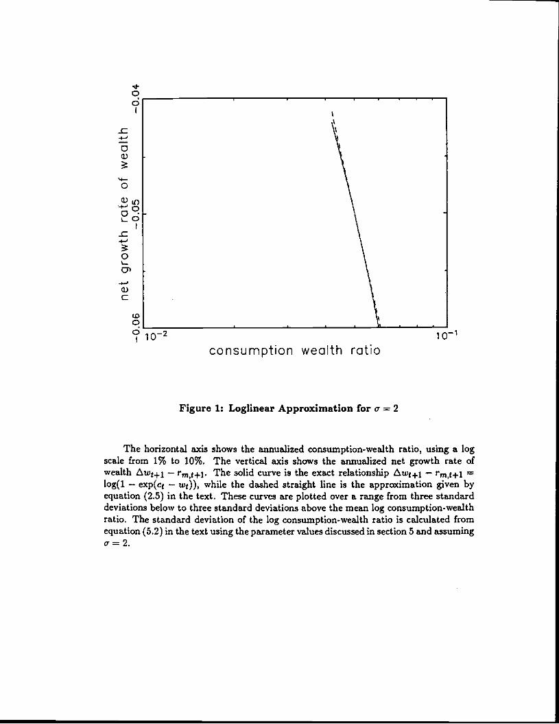
*C

-c

aci)

0

•tCLO-c

0

-Ia.)C

toq1 10-2 10_I

consumption wealth ratio

Figure 1: Loglinear Approximation for a = 2

The horizontal axis shows the annualized consumption-wealth ratio, using a logscale from 1% to 10%. The vertical axis shows the annualized net growth rate ofwealth Awj+i — rmj+I. The solid curve is the exact relationship iwg — rmg÷1 =log(1 — exp(ct — wj)), while the dashed straight line is the apprwcimation given byequation (2.5) in the text. These curves are plotted over a range from three standarddeviations below to three standard deviations above the mean log consumption-wealthratio. The standard deviation of the log consumption-wealth ratio is calculated fromequation (5.2) in the text using the parameter values discussed in section 5 and assuminga=2.

(N00

-c-4-,

o.4-0

0-c-J

SaD0.4I

I)C

010_i

consumption wealth ratio

Figure 2: Loglinear Approximation for = 4

The horizontal axis shows the annualized consumption-wealth ratio, using a logscale from 1% to 10%. The vertical axis shows the annualized net growth rate ofwealth Aw1 — rm,t+1. The solid curve is the exact relationship awj+i — =log(1 — exp(ct — wg)), while the dashed straight line is the approximation given byequation (2.5) in the text. These curves are plotted over a range from three standarddeviations below to three standard deviations above the mean log consumption-wealthratio. The standard deviation of the log consumption-wealth ratio is calculated fromequation (5.2) in the text using the parameter values discussed in section 5 and assumingc=4.

\

1o2

Number Author Title Date

3924 David Harris Income Shifting in U.S. Multinational 12191

Randall Morck CorporationsJoel SlemrodBernard Yeung

3925 Rosanne Altshuler The Effects of U.S. Tax Policy on the 12/91T. Scott Newlon Income Repatriation PaLtems of U.S.

Multinational Corporations

3926 Frank R. Lichtenberg Labor Market Institutions. Liquidity 12/91

Constraints, and Macroeconomic Stability3927 Lawrence F. Katz Changes in Relative Wages. 1963-1987: 12/91

Kevin M. Murphy Supply and Demand Factors

3928 Daniel S. Hamermesh The Appointment-Book Problem and Commitment. 12,91with Applications to Refereeing and Medicine

3929 Benjamin M. Friedman How Does It Matter? 12191

3930 James R. Hines Jr. On the Sensitivity of R & D to Delicate Tax 12191Changes: The Behavior of U.S. Multinationalsin the 1980s

3931 Bernard Dumas How Long Do Unilateral Target Zones Last? 12,91Lars E.O. Svensson

3932 Andrew B. Lyon Consumption Taxes in a Life-Cycle 12i91Robert M. Schwab Framework: Are Sin Taxes Regressive?

3933 Donald Haurin Local House Price Indexes: 1982-1991 12191Patric HendershotiDon gwook Kim

3934 Frederic S. Mishkin Anatomy of a Financial Crisis 12j91

3935 Donald Siegel Errors in Output Deflalors Revisited: 12/91Unit Values and the PPI

3936 David Romer Openness and Inflation: Theory and Evidence 12191

3937 Mark Schasijcerman Revisions of Investment Plans and the 12191Stock Market Rate of Return

3938 Jonathan Skinner Individual Retirement Accounts: A 12191Review of the Evidence

3939 David H. Good The Suucture of Production. Technical Change 12/91M. Ishaq Nadiri and Efficiency in a Multi-Product Industry:Robin C. Slcides An Application to U.S. Airlines

Number Author 'flUe Date

3940 James M. Poterba Why Didn't the Tax Reform Act of 1986 12/91Raise Corporate Taxes?

3941 Robert P. Inman Fiscal Federalism in Europe: Lessons 12)91Daniel L. Rubinleld From the United States Experience

3942 Paul Asquith Anatomy of Financial Distress: An 12/91Robert Geitner Examination of Junk-Bond IssuersDavid Scharfstcin

3943 Maurice Obstfeld The Adjustment Mechanism 12/91

3944 Alessandro Missale The Debt Burden and Debt Maturity 12/91Olivier Jean Blanchard

3945 Leslie B. Papke Tax Policy and Urban Development: 12/91Evidence From an Enterprise Zone Program

3946 Joseph B. Gagnon How Pervasive is the Product Cycle? 01/92Andrew K. Rose The Empirical Dynamics of American and

Japanese Trade flows

3947 Dank Rodrik The Rush to Free Trade in the Developing World: 01/92Why So Late? Why Now? Will It Last?

3948 John F. Helliwdll Convergence and Growth Linkages Between 01i92Alan Clung North and South

3949 Tarnim Bayoumi Shocking Aspects of European Monetary 01/92Barry Eichengreen Unification

3950 Tanilm Bayoumi Is There a Conflict Between BC Enlargement 01/92Barry Bichengreen and European Monetary Unification?

395! Kathryn M. Dominguez The Role of International Organizations 01)92in the Bretlon Woods System

3952 Janet Currie Is Arbitiation Addictive? Evidence From the 01192Heruy S. Farber Laboratory and the Field

3953 Joshua Aizenman Exchange Rate flexibility. Volatility, and the 01)92Patterns of Domestic and Foreign Direct investment

3954 Zvi Bodie Labor Supply Flexibility and Portfolio Choice 01/92Robert C. Merton in a Life-Cycle ModelWilliam F. Samuelson

3955 Thaohui Chen Estimating Expected Exchange Rates Under 01/92Alberto Giovannini Target Zones

Number Author Title

3956 Bronwyn H. Hall Exploring the Relationship Between R&D and 01/92Jacques Mairesse Productivity in French Manufacturing Firms

3957 Edward E. Learner Testing Trade Theory 01/92

3958 Louis Kaplow A Model of Optimal Complexity of Rules 01/92

3959 Stile Oiler Have Commercial Banks Ignored History? 01/92

3960 Stile Oiler External Shocks, Politics and Private lnvesment: 01/92Dani Rodrik Some Theory and Empirical Evidence

3961 Sule Oiler Bank Exposure. Capital and Secondary Martet 01/92

Harry Huizinga Discounts On Developing Country Debt

3962 Martin Feldstein Social Security Rules and Marginal Tax Rates 01/92Andrew Samwick

3963 James M. Poterba Taxation and Housing: Old Questions. New Answers 01/92

3964 David M. Culler Rising Inequality? Changes in the Distibution of 01/92Lawrence F. Katz Income and Consumption in the 1980s

3965 Victor Zarnowitz Twenty-two Years of the NBER-ASA Quarterly 01/92Philip Braun Economic Outlook Surveys: Aspects and Comparisons

of Forecasting Performance

3966 Martin Feldsteln The Budget and Trade Deficits Arerft Really Twins 01)92

3967 Alan J. Auerbach On the Design and Reform of Capital Gains Taxation 01/92

3968 Alberto Alesina Menus of Linear Income Tax Schedules 01)92Philippe Weil

3969 Robert J. Gordon Measuring the Aggregate Price Level: Implications 01)92For Economic Performance and Policy

3970 Charles R. Hulten What is Productivity: Capacity or Welfare 01/92Measurement?

3971 Charles R. Hulten Growth Accounting When Technical Change is 01/92Embodied in Capital

3972 George J. Borjas The Intergenerational Mobility of Immigrants 01/92

3973 David E Bloom The Fall in Private Pension Coverage in the U.s. 01/92Richard B. Freeman

3974 Lawrence J. Christiano Liquidity Effects and the Monetary Transmission 01/92Martin Eichenbaum Mechanism

Number Author Title Date

3975 Philippe Weil Equilibrium Asset Prices With Undiversifiable Labor 01/92Income Risk

3976 Miles Kimball Precautionary Saving and Consumption Smoothing 01/92Philippe Well Across Time and Possibilities

3977 0. Steven Olley The Dynamics of Productivity in the 01/92Ariel Pakes Telecommunications Equipment Industry

3978 Janet Currie The Impact of Collective Bargaining Legislation 01/92Sheena McConnell On Disputes in the U.S. Public Sector: No Policy

May Be the Worst Policy

3979 Jeffrey I. Bernstein Information Spillovers, Margins. Scale and Scope: 01/92With an Application to Canadian Life Insurance

3980 5. Lad Brainard Sectonl Shifts and Unemployment in Interwar Britain 01/92

3981 Catherine I. Morrison State lnfrastructuie and Productive Performance 01/92Amy Ellen Schwartz

3982 Jeffrey I. Bernstein Puce Margins and Capital Adjustment: Canadian Mill 01/92Products and Pulp and Paper Industries

3983 Laurence Ball Disinflation With Imperfect Credibility 02/92

3984 Morris M. Kielner Do Tougher Licensing Provisions Limit Occupational 02/92Robert T. Kudrle Entry? The Case of Dentistry

3985 Edward Montgomery Pensions and Wage Premia 02/92Kathryn Shaw

3986 Casey B. Mulligan Transitional Dynamics in Two-Sector Modcls of 02/92Xavier Sala-i-Martin Eridogcnous Growth

3987 Theodore Joyce The Consequences and Costs of Maternal Substance 02i92Andrew D. Racine Abuse in New York City: A Pooled Time-Series.Naci Mocan Cross-Section Analysis

3988 Robert J. Gordon Forward Into the Past: Productivity Retrogression 02/92in the Electric Generating Industry

3989 John Y. Campbell Intertemporal Asset Pricing Without Consumption 02/92Data

Copies of the above working papers can be obtained by sending $51X) per copy (plus $1OiX)/orxier for postageand handling for all locations outside the continental U.S.) to Working Papers. NBER, 1050 MassachusettsAvenue. Cambridge. MA 02138. Advance payment is required on all orders. Please make checks payable to theNational Bureau of Economic Research.