An Intertemporal International Asset Pricing Model: … · An Intertemporal International Asset Pricing Model: Theory and Empirical Evidence Jow-ran Chang Department of Quantitative

An Intertemporal International AssetPricing Model: Theory and EmpiricalEvidence

Jow-ran ChangDepartment of Quantitative Finance, National Tsing Hua University

e-mail: [email protected]

Vihang ErrunzaFaculty of Management, McGill University, Montreal


Ked HoganBarclays Global Investors, San Francisco, CA, USA


Mao-wei HungCollege of Management, National Taiwan University


Abstract

We extend Campbell’s (1993) model to develop an intertemporal internationalasset pricing model (IAPM). We show that the expected international asset returnis determined by a weighted average of market risk, market hedging risk, exchangerate risk and exchange rate hedging risk. These weights sum up to one. Our modelexplicitly separates hedging against changes in the investment opportunity set fromhedging against exchange rate changes as well as exchange rate risk from inter-temporal hedging risk. A test of the conditional version of our intertemporal IAPMusing a multivariate GARCH process supports the asset pricing model. We findthat the exchange rate risk is important for pricing international equity returns andit is much more important than intertemporal hedging risk.

Keywords: international finance; asset pricing; currency risk; intertemporal.

JEL classification: G11, G12, G15

We are grateful to Rene Stulz for many insightful comments. We thank Francesca Carrieri, Kris

Jacobs, Darius Miller, Sergei Sarkissian and participants at the AFA 2003 meetings for helpful

suggestions. We are grateful to an anonymous referee and the editor, John Doukas for many

helpful comments. Errunza thanks the SSHRC for financial support. Correspondence: Vihang

Errunza, Faculty of Management, McGill University, 1001 Sherbrooke St. West, Montreal,

Quebec, Canada H3A 1G5.

European Financial Management, Vol. 11, No. 2, 2005, 173–194

# Blackwell Publishing Ltd. 2005, 9600 Garsington Road, Oxford OX4 2DQ, UK and 350 Main Street, Malden, MA 02148, USA.

1. Introduction

Several theoretical international asset pricing models (IAPMs) focus on market riskand currency risk. Well known examples include Solnik (1974) and Adler and Dumas(1983).1 It is widely accepted that the intertemporal nature of the problem is import-ant to consider (Merton, 1973; Stulz, 1981).2 Indeed, in the international setting, ifinvestors hedge their exposure to anticipated variation in the investment opportunityset, both the market hedging risk and the currency hedging risk should be priced inaddition to the market and currency risks. As a first step, Dumas and Solnik (1995)attempt to empirically evaluate the relative importance between exchange rate riskpremia and intertemporal hedging premia.3 They state (p. 476):

We are not in a position to run a test with enough assets. But we can run a ‘horse race’between the two types of models in order to determine which should be our firstpriority: the introduction of hedging risk premia as in the intertemporal, classic APMor the introduction of exchange rate risk premia as in the static, international APM.

Indeed, we are not aware of any existing intertemporal international asset pricing modelthat could be used to conduct a formal test. Hence, there are two primary goals of thispaper. First, we develop a theoretical model that prices market hedging risk and exchangerate hedging risk in addition to market risk and exchange rate risk. This allows us toexplicitly separate hedging against changes in the investment opportunity set from hedgingagainst exchange rate changes as well as separate exchange rate risk from intertemporalhedging risk.4 Second, we test the asset pricing restrictions of our theoretical model, andassess the relative importance between exchange rate risk and hedging risk.

Campbell (1993) develops a domestic asset pricing model in which investors areassumed to be endowed with Kreps-Porteus utility and consumption is substituted outfrom the model.5 He demonstrates that the conditional covariance of any asset returnwith consumption growth can be written in terms of conditional covariances with thereturn on the market and revisions in expectations of future returns on the market.We extend Cambpell’s (1993) model to an international framework in which theinflation rate is time-varying. We employ a recursive preference, which separatesinvestors’ attitudes towards risk from their willingness to substitute future consump-tion for present consumpdtion in pricing international assets.6 Our model prices

1 Empirically, Harvey (1991) rejects the one (market) factor world IAPM, whereas De Santis

and Gerard (1998), Solnik (1997), O’Brien and Dolde (2000) and Carrieri (2001) support

currency risk as a priced factor based on a two (market and currency) factor IAPM.2 Based on a two (market and market hedging) factor CAPM, Chang and Hung (2000), and

Hodrick et al. (2000) conclude that the intertemporal hedging risk is priced.3De Santis and Gerard (1998) conduct an indirect test of the relevance of the intertemporal

component of the model by including the information variables as explanatory variables.4 Our model can be viewed as a special case of the more general model of Stulz (1981).5 This avoids problems of measurement error and time-aggregation arising from aggregate

consumption data.6 Past international asset pricing models assume investors maximise a time-additive, von

Neumann-Morgenstern expected utility of life-time consumption function. This implies that

the two distinct concepts of intertemporal substitution and risk aversion are characterised by

the same parameter.

174 J.-R. Chang, V. Errunza, K. Hogan and M.-W. Hung

# Blackwell Publishing Ltd, 2005

exchange rate risk and exchange rate hedging risk in addition to market risk andmarket hedging risk. While the market hedging risk is the covariance of asset returnswith news about the discounted value of all future market returns, the exchange ratehedging risk is the covariance of asset returns with news about the discounted value ofall future currency returns.

Our main results can be summarised as follows. First, the expected internationalasset return can be expressed as a weighted average of consumption risk, inflation riskand market risk. Second, we use a log-linear approximation of the budget constraintto substitute out consumption to obtain an intertemporal international asset pricingmodel without consumption. We show that the expected international asset return isdetermined by a weighted average of market risk, market hedging risk, exchange raterisk and exchange rate hedging risk. Third, we estimate and test the conditionalversion of our intertemporal IAPM using a multivariate GARCH process. Theevidence supports the international version of the intertemporal asset pricing model.Consistent with Dumas and Solnik (1995) and De Santis and Gerard (1998), we findthat exchange rate risk is important for pricing international equity returns. Further,the exchange rate risk is much more important than intertemporal hedging risk.

The remainder of the paper is organised as follows. Section 2 derives the model ofinternational asset pricing in which investors are endowed with homogeneous prefer-ences. Section 3 constructs a model where investor’s consumption preferences arenationally heterogeneous to derive a generalised intertemporal international assetpricing model. Section 4 discusses the econometric methodology. Data and empiricalresults are discussed in section 5. Section 6 provides a comparison of the contributionof exchange rate risk and intertemporal risk. Section 7 concludes the paper.

2. Portfolio choice in an international setting

In this section, we consider the problem of optimal consumption and portfolioallocation in a unified world capital market without taxes or transactions costs.Investors’ preferences are assumed to be homogeneous and there is the same menuof assets for every investor in all countries. That is to say, everybody face the sameconsumption and investment opportunities and there exists a representative agent inthe world. Therefore, we can formulate a economy where purchase power parity(PPP) holds. Section 3, we will disentangle this assumption to discuss an internationalasset pricing model under the deviation of PPP. Now, we consider a world of Lþ 1countries and a set of S equity securities. All returns are measured in the Lþ 1stcountry’s currency (numeraire) in excess of the risk free rate. To facilitate discussion,we define the following terms:

�t : the price level expressed in the currency of country Lþ 1 at time t.Ri,t : the real return for security i at time t.RN

i;t : the nominal return for security i at time t.Ct : the real consumption at time t.CN

t : the nominal consumption at time t.Rm,t : the real return for market portfolio at time t.RN

m;t : the nominal return for market portfolio at time t.

In this setup, the optimal solution can be obtained by specifying a real pricing kernel,Mtþ1:

Intertemporal International Asset Pricing 175


1 ¼ EtðRi;tþ1Mtþ1Þ; ð1Þ

where Et is the expected value function conditional on the information available to theinvestor at time t.

Note that under perfect foresight the real return links the nominal return toinflation through the Fisher parity equation,

RNi;tþ1

�t�tþ1

¼ Ri;tþ1; ð2Þ

we obtain the pricing formula under time-varying inflation rate,

1 ¼ Et RNi;tþ1

�t�tþ1

Mtþ1

� �: ð3Þ

Furthermore, investors are assumed to have a Kreps-Porteus utility. FollowingEpstein and Zin (1989), it can be shown that the pricing kernel has the following form:

Mtþ1 ¼ �Ctþ1

Ct

� ��1 �=( )�

fRm;tþ1g��1; ð4Þ

where the parameter � is the agent’s subjective time discount factor, � is defined as�¼ (1� �)/[1� (1/�)], and � can be interpreted as the Arrow-Pratt coefficient ofrelative risk aversion. It can also be shown that � measures the elasticity of inter-temporal substitution. For instance, if the agent’s coefficient of relative risk aversion,�, is greater (smaller) than the reciprocal of his elasticity of intertemporal substitution,1/�, then he prefers early (late) resolution of uncertainty. If � is equal to 1/�, theagent’s utility becomes an isoelastic von Neumann-Morgenstern utility and he isindifferent to the timing of the resolution of uncertainty.

Plugging equation (4) into equation (3), we obtain

1 ¼ Et RNi;tþ1

�t�tþ1

�CN

tþ1=�tþ1

CNt =�t

� ��1=�( )�

RNm;tþ1

�t�tþ1

� ��124

35: ð5Þ

Equation (5) is the basic pricing formula. Based on equation (5), we will followCampbell (1993) to substitute consumption out of the pricing formula.

When �¼ 1/�, the Euler equations of the time additive expected utility model arealso obtained under random inflation assumption:

1 ¼ Et RNi;tþ1

�t�tþ1

�CN

tþ1=�tþ1

CNt =�t

� ��1=�( )

ð6Þ

Another special case is the logarithmic risk preference where �¼ 1/�¼ 1. Then, theEuler equations under fixed inflation are same as the Euler equations under randominflation and can be written in two algebraically identical functional forms:

1 ¼ Et RNi;tþ1�

CNtþ1

CNt

� ��1( )

ð7Þ

or



1 ¼ EtfRNi;tþ1=R

Nm;tþ1g ð8Þ

In this case, the parameter � governing intertemporal substitutability can not be identifiedfrom these equations. Hence, under logarithmic risk preferences there is no differencebetween Euler equations of the non-expected utility model and the expected utility model.

If we assume that asset prices and consumption are jointly lognormal or alterna-tively if we assume that asset prices and consumption are conditional homoskedasticand use a second order Taylor expansion, the log-version of the real Euler equation(5) can be represented as:

0 ¼ � log � � ð�=�ÞEt�ctþ1 þ ð�� 1ÞE

trm;tþ1 þ E

tri;tþ1 þ �ðð1=�Þ � 1ÞE

t��tþ1

þ 1

2½ð�=�Þ2Vcc þ ð�� 1Þ2Vmm þ Vii � 2ð�=�Þð�� 1ÞVcm � 2ð�=�ÞVci

þ 2ð�� 1ÞVim� þ1

2f½ð�ðð1=�Þ � 1Þ�2V�� 2�2ð1=�Þðð1=�Þ � 1ÞV�c

þ 2�ð�� 1Þðð1=�Þ � 1ÞV�m þ 2�ðð1=�Þ � 1ÞV�ig (9)

where lowercase letters are used for logs and Vcc denotes vart (ctþ1), Vjj denotes vart(rj,tþ1) 8j¼ i, m, Vcj denotes covt (ctþ1, rj,tþ1) 8j¼ i, m, Vim denotes covt (ri,tþ1, rm, tþ1),Vi�¼ covt (ri, tþ1,r�,tþ1), and r�;tþ1 ¼ d lnð�tþ1Þ ¼ d�tþ1

�tþ1. In equation (9), we do not

assume that asset prices and consumption are conditional homoskedastic. Inother words, the conditional second moments in equation (9) are time-varying.

Replacing the asset i by market portfolio and rearranging, we obtain the relation-ship among expected consumption growth and the expected return on the marketportfolio and expected price level growth:

Et�ctþ1 ¼ � log � þ 1

2½ð�=�ÞVcc þ ��Vmm þ 2ð1� �Þ�ðð1=�Þ � 1ÞV��

� 1

2½2�Vcm þ 2�ðð1=�Þ � 1ÞV�c � 2�ð1� �ÞV�m�

þ �Etrm;tþ1 þ ð1� �ÞE

tr�;tþ1

¼ � log � þ 1

2ð�=�Þvar½�ctþ1 � �rm;tþ! þ ð1� �Þ��tþ!� þ �E

trm;tþ1

þ ð1� �ÞEtr�;tþ1 ð10Þ

As has been noted, the second term in equation (10) is not a constant now.Equation (10) indicates that after adjusting the first and second term in equation(10), consumption growth is linearly related to the expected market return andexpected inflation. In addition, the coefficients of these two variables add up to one.

When we subtract the risk free version of (9) from the general version, we obtain:

eEtri;tþ1 � rf ;tþ1 ¼ �Vii

2þ ð�=�ÞVic þ ð�� ð�=�ÞÞVi� þ ð1� �ÞVimÞ ð11Þ

where rf,tþ1 is a log riskless nominal interest rate. If inflation is fixed or known exante, this result is the same as Campbell (1993). Equation (11) shows that the expectedexcess log return on an asset is a linear combination of its own variance, which isproduced by Jensen’s inequality, and by a weighted average of three covariances. The



weights on the consumption, inflation and market are �/�, (�� (�/�)) and (1� �),respectively which sum up to 1. In Campbell (1993), Vi� is equal zero and the weightson consumption and market are �/� and (1� �) which does not sum up to 1. This isone of the most important differences between Campbell’s model and our randominflation model.

If the objective function is a time-separable power utility function, a real functionalform of the loglinear version consumption CAPM pricing formula can be obtained:

Etri;tþ1 � rf ;tþ1 ¼ �Vii

2þ ð1=�ÞVic þ ð1� ð1=�ÞÞVi� ð12Þ

The weights on the consumption and inflation are 1/� and (1� (1/�)), respectivelythat also sum up to one. However, when the coefficient of relative risk aversion �¼ 1,then �¼ 0, and the model can be collapsed into the real functional form of theloglinear static CAPM which is the same as the nominal structure of the loglinearstatic CAPM.

The representative agent in the world can invest his wealth in Q (¼Lþ S) assetswhich comprise L currencies and S equities. Currencies may be taken to be thenominal bank deposits denominated in the non-numeraire currencies. The represen-tative agent’s dynamic budget constraint under time-varying inflation can be writtenas:

Wtþ1

�tþ1¼ RN

m;tþ1

�t�tþ1

Wt

�t� CN

t

�t

� �ð13Þ

where Wtþ1 is the investor’s nominal wealth at time tþ 1. The budget constraint inequation (13) is nonlinear because of the interaction between subtraction and multi-plication.

Following Campbell (1993), we linearise the budget constraint by dividing equation (13)by Wt, taking the log, and then using a first-order Taylor approximation around themean log consumption/wealth ratio log (C/W).

ctþ1 � Etctþ1 ¼ rm;tþ1 � E

trm;tþ1 þ ð1� �Þð E

tþ1�E

tÞX1j¼1

�jrm;tþ1þj

� ð1� �Þð Etþ1

�EtÞX1j¼1

�jr�;tþ1þj

� 1

2ð�=�Þ

X1j¼‘1

�jfVartþ1½�ctþ1þj � �rm;tþ1þj þ ð1� �Þ��tþ1þj�

� Vart½�ctþ1þj � �rm;tþ1þj þ ð1� �Þ��tþ1þj� ð14Þ

Equation (14) implies that unexpected consumption may come from four sources.The first source is the unexpected return on invested wealth today. The second sourceis the expected future nominal returns that depend on the magnitude of �. When � isless than one, an increase (or decrease) in the expected future nominal return increases(or decreases) the unexpected consumption. Conversely, when � is greater than one,an increase (or decrease) in the expected future nominal return decreases (or increases)the unexpected consumption. The third source is the inflation rate that also dependson the magnitude of �. When � is less than one, an increase (or decrease) in theinflation decreases (or increases) the unexpected consumption. Conversely, when � is



greater than one, an increase (or decrease) in the inflation increases (or decreases) theunexpected consumption.

The last term in equation (14) is related to the conditional variance of marketreturn. Note that in the original model of Campbell (1993), all variances and covari-ances of log asset and consumption are constant through time, and the last term inequation (14) is constant. Campbell (1993) notes several ways in which consumptioncan be subsitituted out of the model with changing variances.7 One of them is to setthe elasticity of intertemporal substitution �¼ 1, then � is infinite, and the conditionalvariance of (14) must be zero. In this case, pricing formula can be derived in anenvironment of conditional heteroskedasticity. However, when we test the modelempirically in the next section, we assume that the conditional variance of marketreturn follows a GARCH process which is uncorrelated with any asset returns.8

Hence, based on equation (14), the conditional covariance of any asset return withconsumption can be rewritten in terms of the covariances with the return on themarket and revisions in expectations of future return on the market and inflation:

covtðri;tþ1;�ctþ1Þ � Vic ¼ Vim þ ð1� �ÞVih � ð1� �ÞVih�; ð15Þ

where, Vih ¼ covt ri;tþ1; ð Etþ1

�EtÞP1j¼1

�jrm;tþ1þj

!

Vih� ¼ covt ri;tþ1; ð Etþ1

�EtÞX1j¼1

�jr�;tþ1þj

!

Substituting equation (15) into equation (11), we obtain an asseat pricing model withrandom price, which is not related to consumption:


2þ �Vim þ ð� � 1ÞVih þ ð1� �ÞVi� þ ð1� �ÞVih� ð16Þ

The only preference parameter that enters equation (16) is the coefficient of relativerisk aversion �. The elasticity of intertemporal substitution � has disappeared fromthis asset pricing model. Equation (16) states that the expected excess log return of anasset, adjusted for a Jensen’s inequality effect, is a weighted average of four covari-ances. The covariances are with the return on the market portfolio, with news aboutfuture returns on invested wealth, with the return from inflation, and with news aboutfuture inflation.

3. The intertemporal international asset pricing model under PPP deviation

In this section, we consider the problem of optimal consumption and portfolioallocation in a unified world capital market where investors’ preferences are assumedto be nationally heterogeneous, but there is the same menu of assets for every investorin all countries. That is to say, there does not exist a representative agent in the world.In this paper, we assume that PPP still hold in each domestic country and there is a

7Relaxing this assumption has no effect on the log-linearisation of the budget constraint and

the formulation of the intertemporal optimisation problem.8Restoy (1991) also extends Campbell (1993) to discuss the case in which the variance of market

return follows a GARCH process.



representative agent in each domestic country. Therefore, we can first deal with arepresentative agent in each country like we do in the section 2, and then aggregateacross countries to obtain a generalised international asset pricing model. We nowturn to the problem of aggregation directly. It is true that different investors may usedifferent sets of information and models to forecast future market returns and infla-tion. To obtain the aggregation results, we first add the superscript l to equation (16)to indicate the optimal condition for investor l who is a representative agent in thecountry l:


2þ �lVl

im þ ð�l � 1ÞVlih þ ð1� �lÞVl

i� þ ð1� �lÞVlih� ð17Þ

Next, we multiply equation (17) by �l, where �l¼ 1/�l and then take an average overall investors, where the weights are the investors’ relative wealth.9

Etri;tþ1 � rf ;tþ1 ¼� Vii

2þ 1

�mVm

im þ 1

�m� 1

� �Xl!lVl

ih

þ 1� 1

�m

� �Xl!lVl

i� þ 1� 1

�m

� �Xl!lVl

ih� ð18Þ

where, �m ¼P

l Wl�l

� �=P

l Wl

� �and !l ¼ ð1��lÞWlP

lð1��lÞWl

.

The drawback is that the third, fourth, and fifth terms of (18) are unobservable. Inthe international setting, they contain the covariances of security i with the hetero-geneous investors’ rate of market return forecasting, rate of inflation, and inflationforecasting. They are weighted by their wealth and by one minus their relative riskaversion. Because it is impossible to measure each individual’s relative risk aversion,we cannot use the wealth and relative risk aversion weighted average rate of marketreturn forecasting, rate of inflation, or inflation forecasting. Since all individuals ofthe same country use the same deflator and we use the national wealth weightedaverage relative risk aversion instead of the individual ones, we have a sum of oneterm per each country.

Several interesting and intuitive results emerge. First, the international asset riskpremium adjusted for one-half its own variance is related to its covariances with:(a) the market portfolio, (b) the aggregate of innovation in discounted expected futuremarket returns from different investors across countries, (c) the aggregate of inflationfrom different countries, and (d) the aggregate of innovation in inflation of differentinvestors, discounted using values for expected future inflation across different coun-tries. The weights are 1/�m, 1/�m� 1, 1� 1/�m, 1� 1/�m, respectively that sum toone.10 Second, the international asset is priced without referring to its covariancewith consumption growth. Third, because consumption has been substituted out, thecoefficient of risk tolerance, �m, is the only preference parameter that enters the assetpricing model – equation (18).

9We follow Adler and Dumas (1983) to deal with the intrinsic problem of aggregation in

international asset pricing.10 The market hedging risk is a weighted average of the market portfolio for investors from

different countries. This is different from the domestic counterpart of Campbell (1993).



If we are willing to make further simplifying assumptions, we can obtain a morecompact result. Specifically, if investors have identical current and future marketportfolio expected returns, we can take an average over all investors, where theweights are their relative wealth, and thus obtain a simple version of the intertemporalinternational asset pricing model:

Etri;tþ1 � rf ;tþ1 ¼� Vii

2þ �mVim þ ð�m � 1ÞVih

þ ð1� �mÞX

l!lVl

i� þ ð1� �mÞX

l!lVl

ih� ð19Þ

where, �m ¼P

l Wl�l

� �=P

l Wl

� �and !l ¼ ð1��lÞWlP

lð1��lÞWl

.

In our model, inflation rate measured in currency of country Lþ 1 contains infla-tion rate in domestic and exchange rate between domestic currency and the currencyof country Lþ 1. Therefore, we should separate our inflation rate measured incurrency of country Lþ 1 to country l’s inflation rate and percentage change inexchange rate. We assume that �Lþ1 is country l’s price level measured in currencyof country Lþ 1, �l is country l’s price level measured in currency of country l, and Sis currency Lþ 1 price of currency l, S $(Lþ 1)/$(l).

�Lþ1tþ1

�Lþ1t

¼�ltþ1

�lt� Stþ1

St

� ln �Lþ1tþ1

� �¼ � ln �ltþ1

� �þ� lnðStþ1Þ

r�Lþ1;tþ1 ¼ r�l ;tþ1 þ re;tþ1

Vli;� ¼ Vl

i;�l þ Vli;e

Therefore, inflation risk includes inflation risk measured in domestic currency andexchange rate risk. If domestic inflation is a stable variable, the only randomcomponent in � is the relative change in the exchange rate between the numerairecurrency and the investor’s home currency. Then, Vl

i� is a pure measure of theexposure of asset i to the exchange rate risk and Vl

ih� is a measure of the exposureof asset i to hedge against the exchange rate risk of the country in which investor lresides.

Equation (19) also states that the exchange rate risk is different from the hedgingrisk. Indeed, if Vih and Vl

i� are significantly large, then their contribution to expectedreturn depends on whether �m is different from one. This may be the reason whyDumas and Solnik (1995) argue that exchange rate risk premium may be equivalent tointertemporal risk premium. Their conjecture is, however, based on an empirical‘horse race’ test between an international model and an intertemporal model.

4. Empirical methodology

In this section, we propose an empirical methodology to examine the theoreticalmodel. First, we adopt the approach of Campbell (1991) to construct a state variablesystem to estimate the market hedging portfolio and currency hedging portfolio. Next,we connect the international intertemproal asset pricing and a dynamic covariancesystem to an econometric model. Finally, we use these two systems as the benchmarkmodel to estimate all the unknown parameters.



A. Vector auto-regressive model

We adopt the vector auto-regressive (VAR) approach of Campbell (1991) and con-struct a state variable system to estimate the market hedging portfolio and thecurrency hedging portfolio. We assume that the market index return, rm, is the firstelement of a K-element state variable vector zt and the currency deposit return, rle, isthe lþ 1 st element, l¼ 1,2,..., L. The other elements of zt are known to the market atthe end of period t and are related to the forecasting of future market returns andcurrency deposit returns. In addition, we assume that all the variables zt are demeanedand that the vector zt follows a first order VAR.

ztþ1 ¼ � zt þ utþ1; ð20Þ

where C is a N�N companion matrix of the VAR. The representation of theVAR as a first-order is not restrictive because a higher-order VAR can always bestacked into first-order companion form as discussed by Schwarz (1978). Then wecan use the first order VAR to generate simple multi-period forecasts of futurereturns as,

Etztþ1þi ¼ �iþ1zt: ð21Þ

Define a K -element constant vector e1 whose first element is one and the otherelements are all zero. Then, rm,t¼ e10zt and rm;tþ1 � E

trm;tþ1 ¼ e10utþ1. Define another

K-element constant vector el whose lþ 1 st element is one and other elements are allzero. Then, rle;t ¼ el0zt and rle;tþ1 � E

trle;tþ1 ¼ el0utþ1.

It follows that the discounted sum of forecast revisions in market returns is,

ð Etþ1

�EtÞX1j¼1

�jrm;tþ1þj ¼ e10X1j¼1

�i�jutþ1

¼ e10��ðI� ��Þ�1utþ1

¼ �0hutþ1; ð22Þ

where, �0h is defined as e10��ðI� ��Þ�1 which measures the importance of each statevariable in forecasting future returns on the market.

Similarly, the discounted sum of forecast revisions in currency deposit returns is,

ð Etþ1

�EtÞX1j¼1

�jrle;tþ1þj ¼ el0X1j¼1

�i�jutþ1

¼ el0��ðI� ��Þ�1utþ1

¼ �0le

0utþ1; ð23Þ

where, �0l0

e is defined as el0 �C (I� �C)�1 which measures the importance of each statevariable in forecasting future returns on the currency deposit.

Thus, equation (18) can now be written as,


2þ �Vim þ ð1� �Þ

XLl¼1

!lVlie þ

XKk¼1

½ð� � 1Þ�h;k

þð1� �ÞPL

l¼1 !l�le;k�Vik: (24)



We define Vik�Vart (ri,tþ1,uk,tþ1), where uk,tþ1 is the kth element of utþ1. Equation (24)implies that the expected log excess return on asset i, adjusted for the effect ofJensen’s inequality, is linear in the covariance of the return with the K factors. Theset of restrictions on the risk prices of the factor is the most important contributionof the intertemporal optimisation problem in the international asset pricing model.For example, the first factor, the innovation in the market return, has a risk priceof � þ ð� � 1Þ�h;1 þ ð1� �Þ

P!l�ll;1. Thus, the international intertemporal model

suggests that priced factors should not be found neither by selecting importantmacroeconomic variables, nor by running a factor analysis on the covariance matrixof returns.

B. Econometric specification

Equation (19) appears to be the natural relation to use in an empirical investigation ofthe intertemporal IAPM because it takes into account the investor’s use of newlyacquired information in creating a portfolio, thus taking into account his hedgingstrategy. The model requires equation (19) to hold for every asset including themarket portfolio, market hedging portfolio, currency portfolio and currency hedgingportfolio. Therefore, we assume that each asset return satisfies the following system ofpricing restrictions:

Etr1;tþ1�rf ;tþ1¼�V11

2þ�V1mþð��1ÞV1hþð1��Þ

XLl¼1

!lVl1eþð1��Þ

XLl¼1

!lVl1eh

..

.

EtrN;tþ1�rf ;tþ1¼�VNN

2þ�VNmþð��1ÞVNhþð1��Þ

XLl¼1

!lVlNeþð1��Þ

XLl¼1

!lVlNeh ð25Þ

where, we replace Vi� and Vi�h in equation (19) with Vie and Vieh because the empiricalevidence shows that for our sample countries, the fluctuations in domestic inflationare almost negligible relative to exchange rate changes.11

Let rt denote the N� 1 time series vector which includes N risky assets,ri 8i¼ 1,...,N. In matrix notation, equation (25) and equation (20) can be re-expressedin terms of random log excess return as,

zt

rt � rf ;t � i

� �¼

�zt�1

� 12hd;t þ � hm;t þ ð� � 1Þhh;t þ ð1� �Þhe;t þ ð1� �Þheh;t

� �þ

ut

�t

� �

"t ¼ut

�t

� �jIt�1 � Nð0;HtÞ;

Ht : ðK þNÞ � ðK þNÞ ¼ H11K�K H12

K�N

H21N�K H22

N�N

" #(26)

where, i is an N� 1 vector of one, Ht is the conditional covariance matrix of assetreturns, hd, t is the diagonal element of H22

N�N which denotes the conditional variance

11Note that DeSantis and Gerard (1998) make the same simplification. Our dataset is also

similar to theirs.



of each risk asset, hm, t is the 1st column of H21N�K which denotes the conditional

covariance of each asset with the market portfolio, hh;t ¼PK

k¼1�h;khk;t denotes theconditional covariance of each asset with the market hedging portfolio,he;t ¼

PLl¼1!

lhlþ1;t denotes the conditional covariance of each asset with the currencyportfolio, heh;t ¼

PLl¼1!

lPK

k¼1�le;khk;t denotes the conditional covariance of each asset

with the currency hedging portfolio, hk, t is the k th column of H21N�K and hlþ1,t is the

lþ 1 st column of H21N�K .

Three tests of asset pricing restrictions as special cases of equation (26) are imple-mented. First, we test the validity of the conditional CAPM that implies that � mustbe significantly different from zero. The null hypothesis of �¼ 0 is tested against thealternative hypothesis � 6¼ 0. Second, the test of market hedging risk, exchange raterisk and exchange rate hedging risk as an important factor in the asset pricing modelis implemented. This test implies that � is not equal to one in equation (26). Other-wise, risk premia of assets are determined only by the covariance with the marketportfolio. As discussed in the theoretical model of Section III, if we only test the priceof market hedging risk, Vih, and currency risk, Vie, we can find that the two risk valueswill be significant or insignificant simultaneously because they all depend on whetheror not relative risk aversion, �, is different from one. Hence, we ultimately want toknow which risk is most important in terms of scale.

Equation (26) follows directly from the system of the intertemporal IAPM. Toimplement the tests of the above hypotheses, the dynamics of the variance-covariancestructure in equation (26) must be specified. A multivariate GARCH process based onthe work of Ding and Engle (1994) is used to obtain a testable version of the model.

For simplicity, we assume that the innovation vector et follows a GARCH(1,1) process.The time-varying conditional covariance matrix therefore can be parameterised as,

Ht ¼ �þ a"t�1"0t�1a

0 þ bHt�1b0; ð27Þ

where, G, a, and b denote (NþK)� (NþK) matrices of parameters. It is difficult toestimate the model due to the large number of unknown parameters. In practice, it isnecessary to further restrict the specification for Ht to obtain a numerically tractableformulation. One useful special case is to assume that both a and b are restricted to bediagonal matrices. In such a parameterisation, the conditional covariance between ei,tand ej,t depends only on past values of ei, t�1�ej, t�1, and not on the products or squaresof other residuals. Therefore, equation (27) can be written in a simple form:

Ht ¼ �þ 0 � "t�1"0t�1 þ ��0 �Ht�1; ð28Þ

where, , � are N� 1 vector which includes the diagonal elements of a and b,respectively, and the symbol * denotes the Hadamard (element by element) matrixproduct. However, the diagonal assumption is still too difficult to estimate, unless wecan again reduce the number of unknown parameters. To this end, we assume that theet process is covariance stationary following Ding and Engle (1994). Consider thefollowing system of equations,

ztrt

� �¼ Et�1

ztrt

� �þ "t "tjIt�1 � Nð0;HtÞ ð29Þ

If the et process is covariance stationary, its unconditional variance-covariance matrixis equal to,



H0 ¼ � � ðii0 � 0 � ��0Þ�1: ð30Þ

Then, equation (28) is replaced by,

Ht ¼ H0 � ðii0 � 0 � ��0Þ þ 0 � "t�1"0t�1 þ ��0 �Ht�1: ð31Þ

In a covariance stationary and diagonal construction with (NþK) assets, thenumber of unknown parameters in the conditional variance equation is reduced to2(NþK). The unconditional variance-covariance matrix, H0, is not directly observa-ble. Here we set it equal to the sample covariance matrix of the return.

We use equations (26) and (31) as the benchmark model. Let be the unknownparameters in the model. Then, under the assumption of conditional normality, thelog-likelihood function can be written as,

lnLð Þ ¼ �TN

2ln 2�� 1

2

XTt¼1

ln jHtð Þj �1

2

XTt¼1

"tð Þ0Htð Þ�1"tð Þ: ð32Þ

We estimate this model and compute all tests using the Quasi-Maximum LikelihoodEstimation (QMLE) approach proposed by Bollerslev and Wooldridge (1992).QMLE estimation provides consistent estimates of the parameters. The standarderrors for the estimated coefficients that are calculated under the normal assumptionneed not be correct if the true data generating process is non-normal. Hence, we usethe robust Lagrange Multiplier (LM) test to test the alternative model.

5. Data and empirical results

We use monthly dollar denominated index returns for the USA, the UK, Germany,Japan, and the world portfolio as reported by Morgan Stanley Capital International(MSCI) to investigate the proposed international asset pricing model. The sampleperiod is from January 1980 through December 1997. We also use Eurocurrency ratesoffered in the interbank market in London for one-month deposits in US dollars, UKpounds, German DM and Japanese yen.

Panel A of Table 1 reports the summary statistics for log index returns computed inUS dollars in excess of returns on the Eurodollar rate. The summary statistics includemeans, standard deviations, skewness, kurtosis, Bera-Jarque (1982) statistics, and thesample correlation. The magnitudes of the means, volatilities and correlations are verysimilar to those previously documented in other studies. The kurtosis values indicatethat the unconditional distribution of excess log returns has heavier tails than thenormal distribution for all countries. Furthermore, the Bera-Jarque statistics alsoshow that the hypothesis of normality is rejected in our sample. Hence, we incorp-orate the heteroskedastic property when we estimate the asset pricing model.

Descriptive statistics for the state variables are reported in panel B of Table 1. Weselect a set of state variables that have been widely used in the literature. Theseinstruments include the logarithm of the monthly MSCI world dividend yield (DIV)and the one-month US T-bill rate (TB) both in excess of the monthly Eurodollar rate.These variables have been found to measure the information that investors use to setprices in the market. For example, Campbell (1996) finds that the dividend yield hassome predictive power for future stock returns. Similarly, Fama and Schwert (1977),Ferson (1989), and Ferson and Harvey (1991) find that the short-term T-bill rate (TB)is capable of predicting monthly returns of stocks and bonds.



We first construct the dynamic behaviour of state variables. Table 2 reports theestimates of the coefficients in the one-lag VAR. The first row of Table 2 reports themonthly forecasting equation for the excess log return of the market portfolio(World). Since there is little serial correlation in the monthly market log return, thecoefficient for the World (�1) is small and insignificant. However, the coefficient forworld dividend yield (DIV) is significantly positive and the short-term T-bill rate (TB)is negative. The second row of Table 2 gives the monthly forecasting equation for thereturn on the currency deposit, £. The coefficient of lagged currency deposit returns isalso small and insignificant. The remaining rows of Table 2 report the dynamics of thestate variables. It can be seen that DIV behaves like a persistent AR(1) process with acoefficient of 0.9928.

As discussed in Section 2, the intertemporal model applied to international financialmarkets implies that the conditional expected log return on any asset is linearlyrelated to the covariance of asset return with market return, the covariance withnews about the discounted value of all future market returns i.e. the hedging portfolioreturn, the covariance with the currency deposit return, and the covariance with newsabout the discounted value of all future currency deposit returns i.e. the currencyhedging portfolio return. If the market risk, news about the discounted value of allfuture market risk, exchange rate risk, and news about the discounted value of allfuture exchange rate risk are the only four relevant factors, the price of covariance

Table 1

Summary statistics of excess log returns

Panel A reports summary statistics for monthly dollar denominated log returns for four countries

and the market portfolio. Panel B reports summary statistics for instrumental variables (in

percentages per month) including the 30-day US T-bill returns (TB), and the logarithm of the

monthly MSCI world dividend yield (DIV). All returns are in excess of returns on the monthly

Eurodollar rate. The sample period is from January 1980 through December 1997.

Panel A: Excess returns

Weightsa Mean(*100) SD(*100) Skewness Kurtosis B–J

USA 0.35 0.3283 4.3762 �1.0290** 5.0485** 266.2657**

UK 0.11 0.2540 5.8702 �0.4888* 1.9517** 42.6871**

Germany 0.04 0.1934 6.1322 �0.4682* 1.3120* 23.2785**

Japan 0.31 0.1374 7.0080 0.0385 0.3476* 1.1354*

World 1 0.2255 4.2165 �0.7831* 2.4313** 74.9264**

*, ** denote statistical significant at the 5, 1% level, respectively.a as of 31 December 1990.

Panel B: Instrumental variables

Mean(*100) SD(*100) Maximum Minimum

World(�1) 0.2173 4.2076 10.5096 �20.1767

£(�1) 0.0518 3.4764 14.2591 �12.6903

DM(�1) �0.1401 3.5097 7.8664 �10.8948

Y(�1) 0.0462 3.5450 10.9511 �11.0821

TB �0.1078 0.0901 0.0441 �0.3916

DIV �90.0291 31.0668 �4.2420 �146.9676



risk � should be significantly positive and significantly greater or less than one. Itshould also be noted that the value of � should not be equal to zero or one.

In order to avoid the measurement error, the econometric system employed simul-taneously estimates the parameters of VAR and the asset pricing model. The resultsare reported in Table 3. Consider the estimates of parameters in the VAR. All theelements in the parameter matrix are similar to the unconstrained estimates that arereported in Table 2. The estimate of � is 3.0884 which is significantly different fromzero. This implies that the conditional expected international asset return varies withmarket volatility. This evidence supports the conditional version of the internationalCAPM. This result is the same as Chan et al. (1992). Next, consider the estimatesof parameters in the multivariate GARCH process. All elements of vectors and �are statistically significant at any conventional level. Moreover, the estimates satisfythe stationary conditions, ijþ �i�j< 1 8i, j, for all the variance and covarianceprocesses.

If the estimate of � is equal to one, the model collapses to the conditional CAPM.Since we have the unrestricted estimates, a Wald test would be a convenient way toproceed. The value of the criterion function is 2 (1)¼ 21.935, which corresponds to ap-value of 0.000. This implies that we can reject the hypothesis that market hedgingdemand, exchange rate risk, and currency hedging demand are not important factorsin pricing international stock returns. In other words, the conditional expectedinternational asset return varies with market volatility, market hedging volatility,

Table 2

VAR summary: dynamics of risk factor

We adopt the Vector Auto-Regressive (VAR) approach from Campbell (1991). We assume that

the real market index return and currency portfolio return are the first and second elements of the

state variable vector zt. The other elements of zt are variables that are known to the market at the

end of the period t and are related to forecasting future market returns. In addition, we assume

that the vector zt follows a first order VAR

Dependent

regressors

variables World(�1) £(�1) DM(�1) Y(�1) TB(�1) DIV(�1) R2

World 0.0088

(0.0740)

�0.1758

(0.1198)

0.1488

(0.1288)

0.1207

(0.1099)

�1.4335

(3.6347)

0.0100

(0.0053)

0.0234

£ �0.0730

(0.0612)

0.1345

(0.0990)

�0.0352

(0.1064)

0.0034

(0.0908)

3.2940

(3.0035)

�0.0045

(0.0044)

0.0216

DM �0.1467

(0.0613)

0.0439

(0.0993)

0.0475

(0.1067)

0.0178

(0.0911)

3.0623

(3.0114)

�0.0015

(0.0044)

0.0374

Y �0.0030

(0.0626)

�0.0347

(0.1013)

0.0951

(0.1088)

0.0599

(0.0929)

�1.4571

(3.0719)

0.0029

(0.0045)

0.0166

TB 0.0011

(0.0009)

�0.0018

(0.0015)

0.0023

(0.0016)

�0.0018

(0.0013)

0.7481

(0.0460)

0.0002

(0.0001)

0.8584

DIV �0.2714

(0.1469)

0.1034

(0.2378)

0.1212

(0.2556)

�0.1537

(0.2181)

�13.6528

(7.2113)

0.9928

(0.0106)

0.9924

Standard errors are in parentheses.



currency volatility and currency hedging volatility simultaneously. This evidencesupports the international version of the intertemporal asset pricing model.

The price of risk that arises from the traditional covariance of an asset’s return withmarket return is � þ ð� � 1Þ�h1 þ ð1� �ÞPL

l¼1

�le1, where �h1 is the first element of �h and

Table 3

Quasi maximum likelihood estimates (QMLE) of international asset pricing

This table reports the estimates of the multivariate GARCH(1,1) Model, combining vector

auto-regression and monthly excess log returns to four equity markets. Each mean equation is

written as

zt

rt � rf ;t � i

� �¼

�zt�1

� 12hd;t þ � hm;t þ ð� � 1Þhh;t þ ð1� �Þhe;t þ ð1� �Þheh;t

� �þ

ut

�t

� �

"t ¼ut

�t

� �jIt�1 � Nð0;HtÞ;

where � denotes the price of the market covariance or coefficient of relative risk aversion. The

conditional covariance matrix is formulated as

Ht ¼ H0 � ðii0 � 0 � ��0Þ þ 0 � "t�1"0t�1 þ ��0 �Ht�1

where and � are a 10� 1 vector of constant.

Parameter estimates

3.0884

(0.4459)

�

rm,t� rf,t 0.2102

(0.0233)

0.9602

(0.0085)

£ 0.1674

(0.0307)

0.9755

(0.0147)

DM 0.1936

(0.0432)

0.9507

(0.0208)

Y 0.1902

(0.0233)

0.9677

(0.0083)

TB 0.2100

(0.0200)

0.9605

(0.0076)

DIV 0.1753

(0.0410)

0.9512

(0.0267)

USA 0.2138

(0.0475)

0.9250

(0.0331)

UK 0.1561

(0.0197)

0.9805

(0.0093)

Germany 0.3063

(0.0270)

0.9484

(0.0098)

Japan 0.3054

(0.0286)

0.9506

(0.0096)



�le1 is the first element of �e. Therefore, this model provides a distinct link between thecoefficient of relative risk aversion, �, and the various prices of risks.

6. Disentangling exchange rate risk from intertemporal hedging risk

In the last section, we use an econometric method to examine whether or not relativerisk aversion, �, is different from one. The result shows that three risk components,which depend on whether or not the value for relative risk aversion, �, is differentfrom one, all significantly explain the cross-section of equity returns in the USA, UK,Germany and Japan. However, we would like to know their relative importance.Table 4 reports the mean of the risk variables for the US, UK, Germany, and Japanequity markets. The traditional international CAPM uses only the market risk andexchange rate risk to price assets, whereas the intertemporal model also compensatesfor market hedging risk and exchange rate hedging risk. Table 4 shows some strikingresults about the risk characteristics of international equity returns. First, we comparethe market risk premium and the exchange rate risk premium for our equity markets.For the US equity market, the market risk is very important for explainingreturn whereas the exchange rate risk is small and not significant. In the otherthree equity markets, we find that although exchange rate risk is less importantthan market risk, it is still an important factor to explain equity market return.

Table 4

Summary of risk premiums

This table reports the annualised means and standard deviations for the risk premiums . The total

premium (TP) is the sum of the market premium (MP), the market hedging premium (MHP), the

currency premium (CP) and currency hedging premium (CHP). The definition of risk premium is

as follows.

TP ¼ �covðri;t; rm;tÞ þ ð� � 1Þcovðri;t; rh;tÞ þ ð1� �ÞP

l!lcovðri;t; rle;tÞ

þ ð1� �ÞP

l!lcovðri;t; rleh;tÞ

MP ¼ �covðri;t; rm;tÞ MHP ¼ ð� � 1Þcovðri;t; rh;tÞCP ¼ ð1� �Þ

Pl!

lcovðri;t; rle;tÞ CHP ¼ ð1� �ÞP

l !lcovðri;t; rleh;tÞ

TP MP MHP CP CHP

USA

Mean 4.3681 5.4035 �1.3546 0.0579 0.2610

SD 1.0023 1.7551 1.3885 0.2067 0.2118

UK

Mean 5.1384 6.9687 �1.2515 �0.7548 0.1760

SD 1.1164 1.7529 1.3188 0.2218 0.2401

Germany

Mean 4.3776 5.6133 �0.2906 �0.9761 0.0316

SD 1.3628 1.7056 1.4192 0.2919 0.2468

Japan

Mean 6.7094 8.0265 �0.7827 �0.9013 0.3688

SD 1.7167 2.2407 1.5124 0.2163 0.2773



These findings are consistent with Dumas and Solnik (1995) and De Santis andGerard (1998) who also find that exchange rate risk is important for pricing interna-tional equity returns.

Second, Dumas and Solnik (1995) claim that exchange rate risk might be proxyingfor market hedging risk. Table 4 also allows a comparison of the magnitudes betweenmarket hedging risk premium and exchange rate risk premium. Except for the USequity market, the exchange rate risk premia are highly significant relative to markethedging risk premia. This might be because we use the US dollar as a currencymeasure, so exchange rate risk become less important for the US equity market.Hence, we can conclude that if PPP is violated, exchange rate risk is a more importantfactor than hedging risk in the international asset pricing model. This implies that theconclusion of Chang and Hung (2000) and Hodrick et al. (2000) which states thathedging risk is important in the international asset pricing model should be reassessedin the presence of exchange rate risk.

Third, DeSantis and Gerard (1998) explain the negative exchange rate risk since onewould be willing to give up larger expected returns for smaller expected returnsbecause currency can provide a hedge to PPP deviation. However, this is a relation-ship of contemporary hedge. Table 4 shows that market risk premium is positive,market hedging risk premium is negative, exchange rate risk premium is negativeexcept for the USA, and exchange rate hedging risk is positive. In addition tocontemporary hedge between exchange rate risk premium and market risk premium,market hedging risk premium and exchange rate hedging risk premium are twointertemporal hedges to market risk premium and exchange rate risk premium. Thatis because future market and future currency returns can provide a hedge to marketand currency returns.

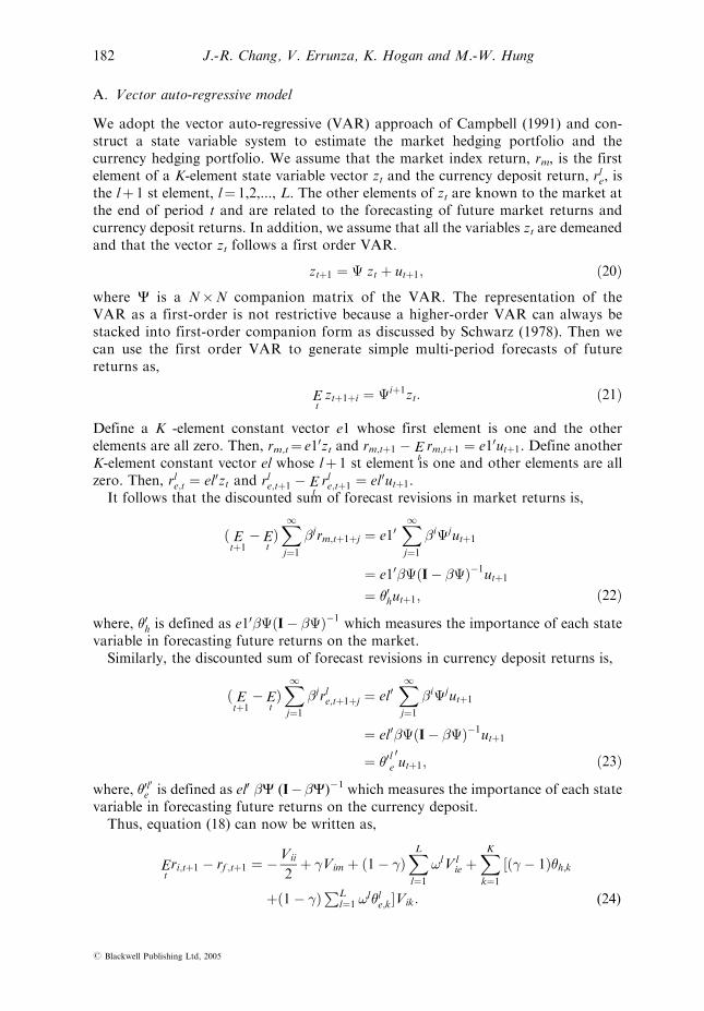
In order to examine the difference between market hedging risk and exchangerate risk over our sample period, we plot the two risks in Figures 1–4. We observelarge increases in market hedging risk associated with the big market drops of1987 and 1990. However, the scale of market hedging risk is smaller than that ofmarket risk. That is because we separate exchange rate risk and exchange rate hedgingrisk from the market hedging risk, and hence the components of exchange rate riskand exchange rate hedging risk absorb some information from market hedging risk.In addition, the pattern of market hedging risk is different from the pattern ofexchange rate risk in all equity markets. Sometimes, we find that market hedgingrisk and exchange rate risk are in a negative relationship, whereas at other times theyshow a positive relationship. Dumas and Solnik (1995) denote that exchange rates canserve as proxies for state variables when constructing intertemporal risk premia,however in our theoretical model we can separate the exchange rate risk and inter-temporal risk into two different risks. Thus, the conclusion of Dumas and Solnik(1995) that exchange rate risk may be equivalent to intertemporal risk needs to bereevaluated.

7. Conclusions

This paper develops an intertemporal IAPM. We use a loglinear approximation of thebudget constraint to obtain an international asset pricing model without consump-tion. The model shows that the expected asset return is determined by a weightedaverage of market risk, market hedging risk, exchange rate risk, and exchange ratehedging risk. The weights are related only to relative risk aversion and sum up to one.



Our model can be viewed as a special case of the pioneering work of Stulz (1981). Ourresults can be contrasted with the work of Adler and Dumas (1983) who assumed aconstant investment opportunity set, and did not deal with market hedging risk andexchange rate hedging risk. We are able to explicitly separate hedging against changesin the investment opportunity set from hedging against exchange rate changes as wellas separate exchange rate risk from intertemporal hedging risk. In our model, theprice of market hedging risk is equal to the negative price of exchange rate risk. Thiscould be the reason why Dumas and Solnik (1995) argue that exchange rate risk is

–0.009

–0.008

–0.007

–0.006

–0.005

–0.004

–0.003

–0.002

–0.001

0

0.001

0.002

1980

1981

1982

1983

1984

1985

1986

1987

1988

1989

1990

1991

1992

1993

1994

1995

1996

1997

Time

Ris

k pr

emiu

m

Intertemporal hedging risk premium

Currency risk premium

Fig. 1. Risk premiums: US equity

1980

1981

1982

1983

1984

1985

1986

1987

1988

1989

1990

1991

1992

1993

1994

1995

1996

1997

Time

Ris

k pr

emiu

m

Intertem poral hedging risk premium


–0.007

–0.006

–0.005

–0.004

–0.003

–0.002

–0.001

0

0.001

Fig. 2. Risk premiums: UK equity



equivalent to market hedging risk. However, their conjecture is based on a ‘horse race’test between the international model and the intertemporal model.

Empirically, we investigate our dynamic international asset pricing model for theUS, UK, Germany and Japan equity markets. Our international model is a four-factor model in which assets are priced using their covariance not only with themarket portfolio and the currency deposit return, but also with the market hedging

–0.005

–0.004

–0.003

–0.002

–0.001

0

0.001

0.002

0.003

1980

1981

1982

1983

1984

1985

1986

1987

1988

1989

1990

1991

1992

1993

1994

1995

1996

1997

Time

Ris

k pr

emiu

m

Intertemporal hedging risk premium


Fig. 3. Risk premiums: Germany equity

–0.005

–0.004

–0.003

–0.002

–0.001

0

0.001

0.002

0.003

0.004

1980

1981

1982

1983

1984

1985

1986

1987

1988

1989

1990

1991

1992

1993

1994

1995

1996

1997

Time

Ris

k pr

emiu

m

Intertemporal hedging risk premiumCurrency risk premium

Fig. 4. Risk premiums: Japanese equity



portfolio and the currency hedging portfolio that account for changes in the investmentset. The evidence supports the hypothesis that the market risk is important in aninternational setting. Furthermore, we can reject the hypothesis that market hedgingdemand, exchange rate risk, and currency hedging demand are not important factors inpricing international stock returns. Thus, the evidence supports the international versionof the intertemporal asset pricing model. Finally, we show that the exchange rate risk isdifferent from market hedging risk and the relationship between exchange rate risk andmarket hedging risk may be positive or negative. This suggests that exchange rate riskand market hedging risk are two different risks in international asset pricing with theexchange rate risk being much more important than market hedging risk.

This paper links the intertemporal asset pricing model of Campbell (1993) andinternational asset pricing model of Adler and Dumas (1983) to construct an inter-national intertemporal asset pricing model. The theoretical model shows that theexpected international asset return is determined by a weighted average of marketrisk, market hedging risk, exchange rate risk and exchange rate hedging risk. In theempirical literature, DeSantis and Gerard (1998) show that currency risk is animportant factor of risk premium. Dumas and Solnik (1995) show that both inter-temporal model and international model can explain the risk premium. In this paper,we propose a unified model of intertemporal risk and currency risk. The results showthat international intertemporal model can not be rejected by our international data.Past empirical tests of international data have relied upon conditional versions of thestatic IAPMs. Indeed, a conditional test of an IAPM should be based on an inter-temporal model. Our IAPM fills this gap.

References

Adler, M. and Dumas, B., ‘International portfolio selection and corporation finance: a synthesis,’

Journal of Finance, Vol. 38, 1983, pp. 925–984.

Bansal, R. D. Hsieh, H, and Viswanathan, S., ‘A new approach to international arbitrage

pricing,’ Journal of Finance, Vol. 48, 1993, pp. 1719–1747.

Bera, A. K. and Jarque, C. M., ‘Model specification tests: a simultaneous approach,’ Journal of

Econometrics, Vol. 20, 1982, pp. 59–82.

Bollerslev, T. and Wooldridge, J. M. ‘Quasi-maximum likelihood estimation and inference

in dynamic models with time-varying covariances,’ Econometrics Reviews, Vol. 11, 1992,

pp. 143–172.

Campbell, J. Y., ‘A variance decomposition for stock returns,’ Economic Journal, Vol. 101,

1991, pp. 157–179.

Campbell, J. Y., ‘Intertemporal asset pricing without consumption data,’ American Economic

Review, Vol. 83, 1993, pp. 487–512.

Campbell, J. Y., ‘Understanding risk and return,’ Journal of Political Economy, Vol. 104, 1996,

pp. 298–345.

Carrieri, F., ‘The effects of liberalization on market and currency risk in the European Union,’

European Financial Management, Vol. 7, 2001, pp. 259–290.

Chan, K. C., Karolyi, G. A. and Stulz, R. M., ‘Global financial markets and the risk premium

on US equity,’ Journal of Financial Economics, Vol. 32, 1992, pp. 137–167.

Chang, J. R. and Hung, M. W., ‘An international asset pricing model with time-varying

hedging risk,’ Review of Quantitative Finance and Accounting, Vol. 15, 2000, pp. 235–257.

Cumby, R. E., ‘Consumption risk and international equity returns: Some empirical evidence,’

Journal of international Money and Finance, Vol. 9, 1990, pp. 182–192.

De Santis, G. and Gerard, B., ‘International asset pricing and portfolio diversification with

time-varying risk,’ Journal of Finance, Vol. 52, 1997, pp. 1881–1912.



De Santis, G. and Gerard, B., ‘How big is the premium for currency risk?’ Journal of Financial

Economics, Vol. 49, 1998, pp. 375–412.

Ding, Z. and Engle, R. F., ‘Large scale conditional covariance matrix modeling, estimation and

testing’ Working Paper (University of California at San Diego, 1994.

Dumas, B. and Solnik, B., ‘The world price of foreign exchange rate risk,’ Journal of Finance,

Vol. 50, 1995, pp. 445–479.

Epstein, L. G. and Zin, S. E., ‘Substitution, risk aversion, and the temporal behavior of

consumption and asset returns: a theoretical framework,’ Econometrica, Vol. 57, 1989,

pp. 937–969.

Epstein, L. G. and Zin, S. E., ‘Substitution, risk aversion, and the temporal behavior of

consumption and asset returns: an empirical analysis,’ Journal of Political Economy, Vol. 99,

1991, pp. 263–286.

Fama, E. F. and Schwert, G. W., ‘Asset returns and inflation,’ Journal of Financial Economic,

Vol. 5, 1977, pp. 115–1461.

Ferson, W., ‘Changes in expected security returns, risk, and the level of interest rates,’ Journal

of Finance, Vol. 44, 1989, pp. 1191–1217.

Ferson, W. and Harvey, C. R., ‘Variation of economic risk premiums,’ Journal of Political

Economy, Vol. 99, 1991, pp. 385–415.

Ferson, W. and Harvey, C. R., ‘The risk and predictability of international equity returns,’

Review of Financial Studies, Vol. 6, 1993, pp. 527–567.

Giovannini, A. and Weil, P., ‘Risk aversion and intertemporal substitution in the capital asset

pricing model,’ (NBER, 2824, 1989).

Harvey, C. R., ‘The world price of covariance risk,’ Journal of Finance, Vol. 46, 1991, pp. 111–157.

Hodrick, R. J., Ng, D. and Sengmueller, P., ‘An international dynamic asset pricing model,’

International Tax and Public Finance, Vol. 6, no. 4, 2000, pp. 597–620.

Kreps, D. and Porteus, E., ‘Temporal resolution of uncertainty and dynamic choice theory,’

Econometrica, Vol. 46, 1978, pp. 185–200.

Korajczyk, R. and Viallet, C., ‘An empirical investigation of international asset pricing,’ Review

of Financial Studies, Vol. 2, 1989, pp. 553–585.

Merton, R. C., ‘An intertemporal capital asset pricing model,’ Econometrica, Vol. 41, 1973,

pp. 867–887.

Narayana, K., ‘Disentangling the coefficient of relative risk aversion from the elasticity

of intertemporal substitution: an irrelevance result,’ Journal of Finance, Vol. 45, 1990,

pp. 175–190.

O’Brien, T. and Dolde, W., ‘A currency index global capital asset pricing model,’ European

Financial Management, Vol. 6, 2000, pp. 7–18.

Restoy, F., ‘Optimal portfolio policies under time-dependent returns,’ unpublished manuscript

(Harvard University, 1991).

Ross, S. A., ‘The arbitrage theory of capital asset pricing,’ Journal of Economic Theory, Vol. 13,

1976, pp. 341–360.

Solnik, B., ‘The world price of foreign exchange risk: some synthetic comments,’ European

Financial Management, Vol. 3, 1997, pp. 9–22.

Solnik, R. E., ‘An equilibrium model of the international capital market,’ Journal of Economic

Theory, Vol. 8, 1974, pp. 500–524.

Stulz, R. M., ‘A model of international asset pricing,’ Journal of Financial Economics, Vol. 9,

1981, pp. 383–406.

Stulz, R. M., ‘Pricing capital assets in an international setting: an introduction,’ Journal of

International Business Studies, Winter 1984, pp. 55–73.

Svensson, L. E. O., ‘Portfolio choice with non-expected utility in continuous time,’ Economics

Letters, Vol. 30, 1989, pp. 313–317.

Weil, P., ‘The equity premium puzzle and the risk free rate puzzle,’ Journal of Monetary

Economic, Vol. 24, 1989, pp. 401–421.



Documents

An Intertemporal International Asset Pricing Model: … · An Intertemporal International Asset Pricing Model: Theory and Empirical Evidence Jow-ran Chang Department of Quantitative