Asset Pricing - Chapter VII. The Capital Asset Pricing ... for... · 7.7 The Zero-Beta Capital Asset Pricing Model (Equilibrium) ... Asset Pricing Chapter VII. The Capital Asset Pricing

7.1 Introduction7.2 The Traditional Approach to the CAPM

7.3 Valuing Risky Cash Flows with the CAPM7.4 The Mathematics of the Portfolio Frontier: Many Risky Assets and No Risk-Free Asset

7.5 Characterizing Efficient Portfolios (No Risk-Free Assets)7.6 Background for Deriving the Zero-Beta CAPM: Notion of a Zero Covariance Portfolio

7.7 The Zero-Beta Capital Asset Pricing Model (Equilibrium)7.8 The Standard CAPM

7.9 What have we accomplish?7.10 Conclusions

Asset PricingChapter VII. The Capital Asset Pricing Model: Another View

About Risk

June 20, 2006

Asset Pricing






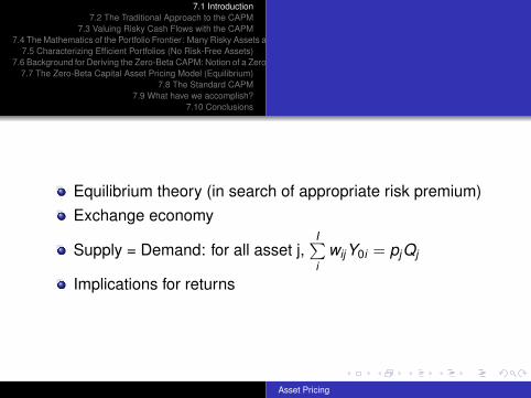
Equilibrium theory (in search of appropriate risk premium)Exchange economy

Supply = Demand: for all asset j,I∑i

wijY0i = pjQj

Implications for returns

Asset Pricing






Proof of the CAPM relationship Appendix 7.1

Traditional Approach

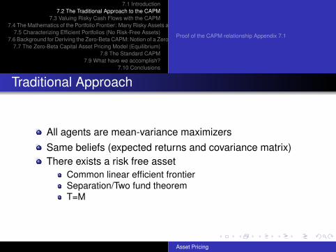
All agents are mean-variance maximizersSame beliefs (expected returns and covariance matrix)There exists a risk free asset

Common linear efficient frontierSeparation/Two fund theoremT=M

Asset Pricing







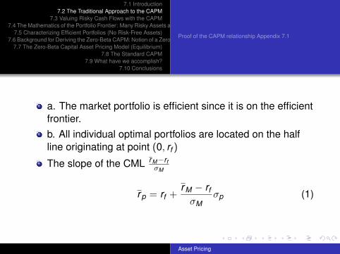
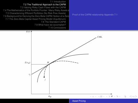
a. The market portfolio is efficient since it is on the efficientfrontier.b. All individual optimal portfolios are located on the halfline originating at point (0, rf )

The slope of the CML rM−rfσM

rp = rf +rM − rf

σMσp (1)

Asset Pricing







s

E (r)

rf

M

sM

CML

E (rM)

j

Asset Pricing







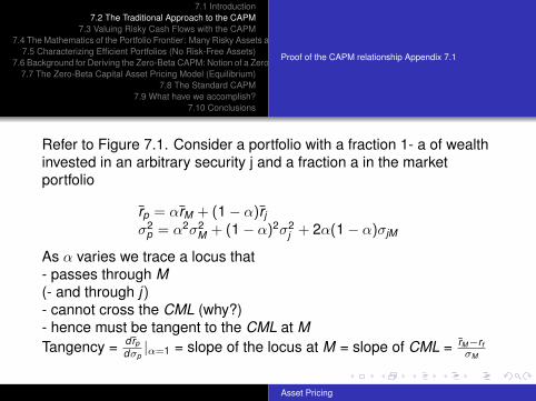
Refer to Figure 7.1. Consider a portfolio with a fraction 1- a of wealthinvested in an arbitrary security j and a fraction a in the marketportfolio

r̄p = αr̄M + (1− α)r̄jσ2

p = α2σ2M + (1− α)2σ2

j + 2α(1− α)σjM

As α varies we trace a locus that- passes through M(- and through j)- cannot cross the CML (why?)- hence must be tangent to the CML at MTangency = dr̄p

dσp|α=1 = slope of the locus at M = slope of CML = r̄M−rf

σM

Asset Pricing







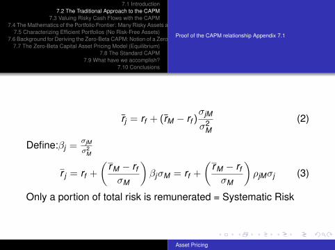
r̄j = rf + (r̄M − rf )σjM

σ2M

(2)

Define:βj =σjM

σ2M

r j = rf +

(rM − rf

σM

)βjσM = rf +

(rM − rf

σM

)ρjMσj (3)

Only a portion of total risk is remunerated = Systematic Risk

Asset Pricing







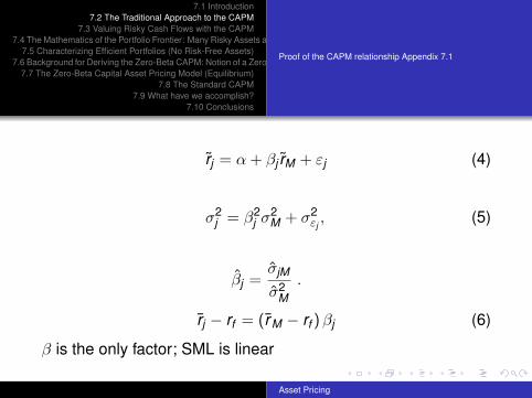
r̃j = α + βj r̃M + εj (4)

σ2j = β2

j σ2M + σ2

εj, (5)

β̂j =σ̂jM

σ̂2M

.

r̄j − rf = (r̄M − rf ) βj (6)

β is the only factor; SML is linear

Asset Pricing







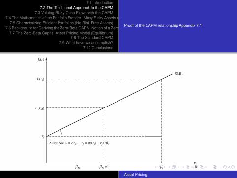
b

E(r)

rf

bM

SML

E(rM)

bM =1

E(ri)

Slope SML = ErM – rf = (E(ri) – rf) /bi

bi

Asset Pricing






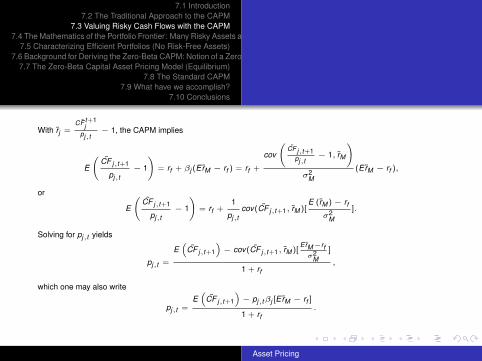
With r̃j =CF̃ t+1

jpj,t

− 1, the CAPM implies

E

C̃F j,t+1

pj,t− 1

!= rf + βj (Er̃M − rf ) = rf +

cov

C̃F j,t+1

pj,t− 1, r̃M

!σ2

M

(Er̃M − rf ),

or

E

C̃F j,t+1

pj,t− 1

!= rf +

1

pj,tcov(C̃F j,t+1, r̃M )[

E (r̃M )− rfσ2

M

].

Solving for pj,t yields

pj,t =

E“

C̃F j,t+1

”− cov(C̃F j,t+1, r̃M )[

Er̃M−rfσ2

M]

1 + rf,

which one may also write

pj,t =E“

C̃F j,t+1

”− pj,t βj [Er̃M − rf ]

1 + rf.

Asset Pricing






Proposition 7.1Proposition 7.2

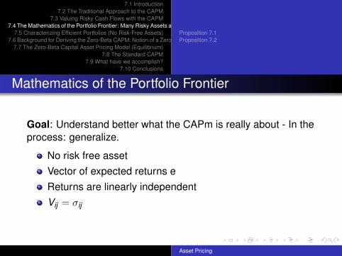
Mathematics of the Portfolio Frontier

Goal: Understand better what the CAPm is really about - In theprocess: generalize.

No risk free assetVector of expected returns eReturns are linearly independentVij = σij

Asset Pricing







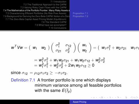
wT Vw =(

w1 w2) (

σ21 σ12

σ21 σ22

) (w1w2

)=

(w1σ

21 + w2σ21 w1σ12 + w2σ

22

) (w1w2

)= w2

1 σ21 + w1w2σ21 + w1w2σ12 + w2

2 σ22

= w21 σ2

1 + w22 σ2

2 + 2w1w2σ12 ≥ 0

since σ12 = ρ12σ1σ2 ≥ −σ1σ2.

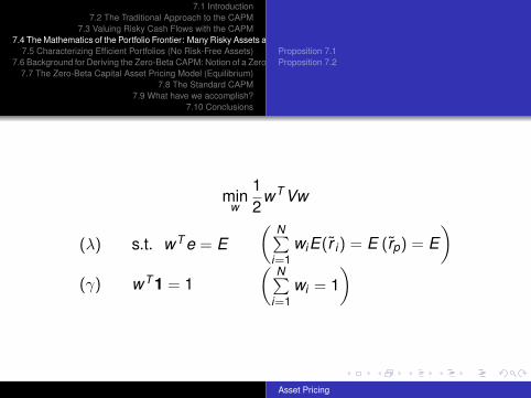
Definition 7.1 A frontier portfolio is one which displaysminimum variance among all feasible portfolioswith the same E(r̃p)

Asset Pricing







minw

12

wT Vw

(λ)

(γ)

s.t. wT e = E

wT 1 = 1

(N∑

i=1wiE(r̃ i) = E (r̃p) = E

)(

N∑i=1

wi = 1)

Asset Pricing







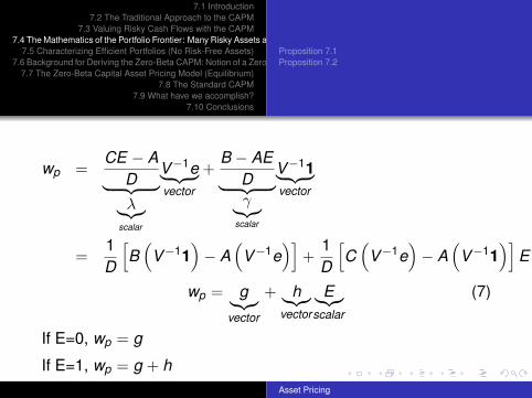
wp =CE − A

D︸︷︷︸λ︸︷︷︸

scalar

V−1e︸︷︷︸vector

+B − AE

D︸︷︷︸γ︸︷︷︸

scalar

V−11︸︷︷︸vector

=1D

[B

(V−11

)− A

(V−1e

)]+

1D

[C

(V−1e

)− A

(V−11

)]E

wp = g︸︷︷︸vector

+ h︸︷︷︸vector

E︸︷︷︸scalar

(7)

If E=0, wp = g

If E=1, wp = g + hAsset Pricing







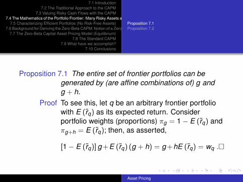
Proposition 7.1 The entire set of frontier portfolios can begenerated by (are affine combinations of) g andg + h.

Proof To see this, let q be an arbitrary frontier portfoliowith E (r̃q) as its expected return. Considerportfolio weights (proportions) πg = 1− E (r̃q) andπg+h = E (r̃q); then, as asserted,

[1− E (r̃q)] g+E (r̃q) (g + h) = g+hE (r̃q) = wq .�

Asset Pricing







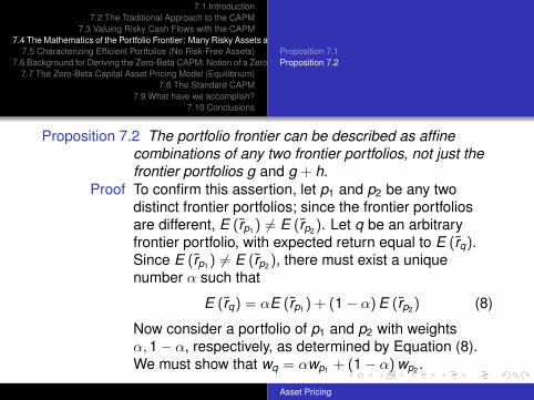
Proposition 7.2 The portfolio frontier can be described as affinecombinations of any two frontier portfolios, not just thefrontier portfolios g and g + h.

Proof To confirm this assertion, let p1 and p2 be any twodistinct frontier portfolios; since the frontier portfoliosare different, E (r̃p1) 6= E (r̃p2). Let q be an arbitraryfrontier portfolio, with expected return equal to E (r̃q).Since E (r̃p1) 6= E (r̃p2), there must exist a uniquenumber α such that

E (r̃q) = αE (r̃p1) + (1− α) E (r̃p2) (8)

Now consider a portfolio of p1 and p2 with weightsα, 1− α, respectively, as determined by Equation (8).We must show that wq = αwp1 + (1− α) wp2 .

Asset Pricing







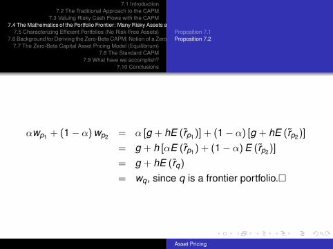
αwp1 + (1− α) wp2 = α [g + hE (r̃p1)] + (1− α) [g + hE (r̃p2)]

= g + h [αE (r̃p1) + (1− α) E (r̃p2)]

= g + hE (r̃q)

= wq, since q is a frontier portfolio.�

Asset Pricing







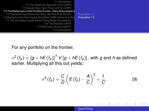
For any portfolio on the frontier,

σ2 (r̃p) = [g + hE (r̃p)]T V [g + hE (r̃p)] , with g and h as definedearlier. Multiplying all this out yields;

σ2 (r̃p) =CD

(E (r̃p)− A

C

)2

+1C

, (9)

Asset Pricing







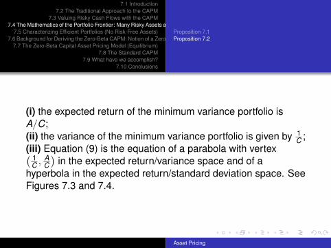
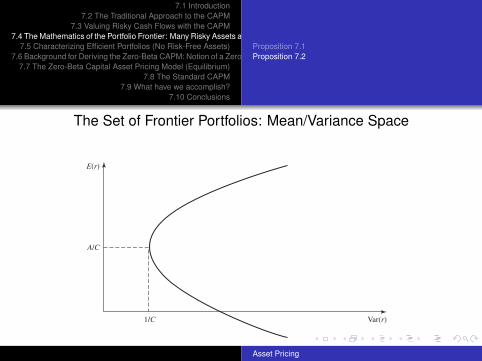
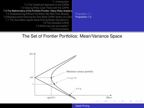
(i) the expected return of the minimum variance portfolio isA/C;(ii) the variance of the minimum variance portfolio is given by 1

C ;(iii) Equation (9) is the equation of a parabola with vertex( 1

C , AC

)in the expected return/variance space and of a

hyperbola in the expected return/standard deviation space. SeeFigures 7.3 and 7.4.

Asset Pricing







The Set of Frontier Portfolios: Mean/Variance Space

Var(r)

E(r)

1/C

A/C

Asset Pricing







The Set of Frontier Portfolios: Mean/Variance Space

SD(r)

E(r)

sqr(1/C )

A/C

Minimum variance portfolio

w = g + h

w = g

1

Asset Pricing







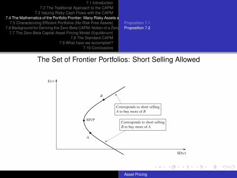
The Set of Frontier Portfolios: Short Selling Allowed

SD(r)

E(r)

MVP

A

B

Corresponds to short selling

A to buy more of B

Corresponds to short selling

B to buy more of A

Asset Pricing






Definition 7.2Proposition 7.3Proposition 7.4

Efficient Portfolios: Characteristics

Definition 7.2: Efficient portfolios are those frontier portfoliosfor which the expected return exceeds A/C, the expectedreturn of the minimum variance portfolio.

Asset Pricing







Proposition 7.3 Any convex combination of frontier portfolios is also a frontier portfolio

Proof Let (w̄1...w̄N ), define N frontier portfolios (w̄i represents the vector defining the compositionof the i th portfolio) and αi , t =, ..., N be real numbers such that

PNi=1 αi = 1. Lastly, let

E (r̃i ) denote the expected return of the portfolio with weights w̄i . The weightscorresponding to a linear combination of the above N portfolios are:

NXi=1

αi w̄i =NX

i=1

αi (g + hE (r̃i ))

=NX

i=1

αi g + hNX

i=1

αi E (r̃i )

= g + h

24 NXi=1

αi E (r̃i )

35

ThusNP

i=1αi w̄i is a frontier portfolio with E (r) =

NPi=1

αi E (r̃i ). �

Asset Pricing







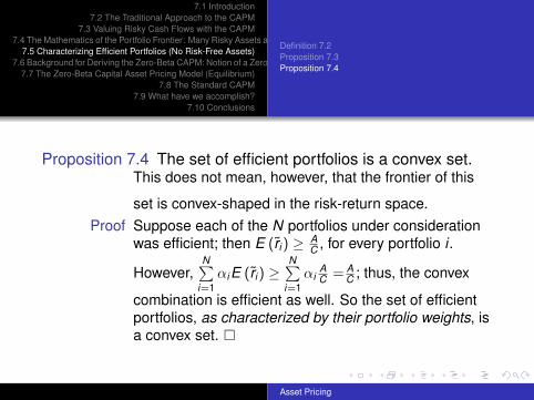
Proposition 7.4 The set of efficient portfolios is a convex set.This does not mean, however, that the frontier of this

set is convex-shaped in the risk-return space.Proof Suppose each of the N portfolios under consideration

was efficient; then E (r̃i) ≥ AC , for every portfolio i .

However,N∑

i=1αiE (r̃i) ≥

N∑i=1

αiAC = A

C ; thus, the convex

combination is efficient as well. So the set of efficientportfolios, as characterized by their portfolio weights, isa convex set. �

Asset Pricing






Proposition 7.5

Proposition 7.5 For any frontier portfolio p, except the minimumvariance portfolio, there exists a unique frontierportfolio with which p has zero covariance.We will call this portfolio the zero covarianceportfolio relative to p, and denote its vector ofportfolio weights by ZC (p).

Proof by construction

Asset Pricing






Proposition 7.5

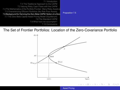
The Set of Frontier Portfolios: Location of the Zero-Covariance Portfolio

Var(r)

E(r)

MVP

p

(1/C )

A/C

ZC( p)E[rZC( p)]

Asset Pricing






Proposition 7.5

Let q be any portfolio (not necessary on the frontier) and let pbe any frontier portfolio.

E(r̃j)

= E(r̃ZC(M)

)+ βMj

[E (r̃M)− E

(r̃ZC(M)

)](10)

Asset Pricing






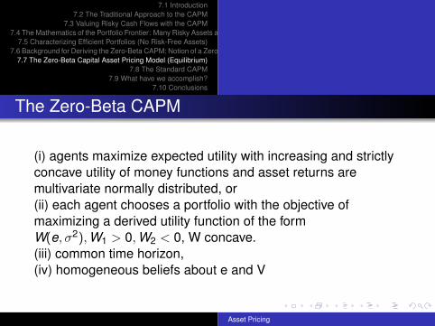
The Zero-Beta CAPM

(i) agents maximize expected utility with increasing and strictlyconcave utility of money functions and asset returns aremultivariate normally distributed, or(ii) each agent chooses a portfolio with the objective ofmaximizing a derived utility function of the formW(e, σ2), W1 > 0, W2 < 0, W concave.(iii) common time horizon,(iv) homogeneous beliefs about e and V

Asset Pricing






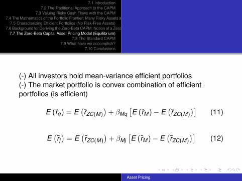
(-) All investors hold mean-variance efficient portfolios(-) The market portfolio is convex combination of efficientportfolios (is efficient)

E (r̃q) = E(r̃ZC(M)

)+ βMq

[E (r̃M)− E

(r̃ZC(M)

)](11)

E(r̃j)

= E(r̃ZC(M)

)+ βMj

[E (r̃M)− E

(r̃ZC(M)

)](12)

Asset Pricing






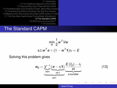
The Standard CAPM

minw

12

wT Vw

s.t.wT e + (1− wT 1)rf = E

Solving this problem gives

wp = V−1︸︷︷︸nxn

(e − rf 1)︸︷︷︸nx1︸︷︷︸

nx1

E (r̃p)− rf

H︸︷︷︸a number

(13)

Asset Pricing






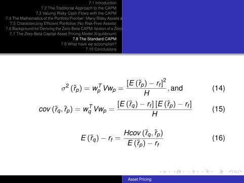
σ2 (r̃p) = wTp Vwp =

[E (r̃p)− rf ]2

H, and (14)

cov (r̃q, r̃p) = wTq Vwp =

[E (r̃q)− rf ] [E (r̃p)− rf ]

H(15)

E (r̃q)− rf =Hcov (r̃q, r̃p)

E (r̃p)− rf(16)

Asset Pricing






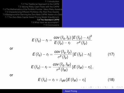
E (r̃q)− rf =cov (r̃q, r̃p)

E (r̃p)− rf

[E (r̃p)− rf ]2

σ2 (r̃p)

or

E (r̃q)− rf =cov (r̃q, r̃p)

σ2 (r̃p)[E (r̃p)− rf ] (17)

E (r̃q)− rf =cov (r̃q, r̃M)

σ2 (r̃M)[E (r̃M)− rf ] ,

orE (r̃q) = rf + βqM [E (r̃M)− rf ] (18)

Asset Pricing






What have we accomplish?

The pure mathematics of the mean-variance portfoliofrontier goes a long way.In particular in producing a SML - like relationship whereany frontier portfolio and its zero -covariance kin are theheroesThe CAPM = a set of hypothesis guaranteeing that theefficient frontier is relevant (mean-variance optimizing) andthe same for everyone (homogeneous expectations andidentical horizons)

Asset Pricing






The implication: every investor holds a mean-varianceefficient portfolioSince the efficient frontier is a convex set, this implies thatthe market portfolio is efficient. This is the key lesson of theCAPM. It does not rely on the existence of a risk free asset.The mathematics of the efficient frontier then produces theSML.In the process, we have obtained easily workable formulaspermitting to compute efficient portfolio weights with orwithout risk-free asset.

Asset Pricing






Conclusions

The asset management implications of the CAPMThe testability of the CAPM: what is M? the fragility ofbetas to this definition ( The Roll Critique)The market may not be the only factor (Fama-French)remains: do not bear diversifiable risk

Asset Pricing

Documents

Asset Pricing - Chapter VII. The Capital Asset Pricing ... for... · 7.7 The Zero-Beta Capital Asset Pricing Model (Equilibrium) ... Asset Pricing Chapter VII. The Capital Asset Pricing