arX

iv:a

stro

-ph/

0103

390v

1 2

3 M

ar 2

001

Observational Tests and Predictive Stellar Evolution

P. A. Young, E. E. Mamajek, David Arnett and James Liebert

Steward Observatory, University of Arizona, 933 N. Cherry Avenue, Tucson AZ 85721

payoung@as.arizona.edu, eem@as.arizona.edu, darnett@as.arizona.edu,

jliebert@as.arizona.edu

ABSTRACT

We compare eighteen binary systems with precisely determined radii and masses

from 23 to 1.1 M⊙, and stellar evolution models produced with our newly revised code

TYCHO. “Overshooting” and rotational mixing were suppressed in order to establish a

baseline for isolating these and other hydrodynamic effects. Acceptable coeval fits are

found for sixteen pairs without optimizing for heavy element or helium abundance. The

precision of these tests is limited by the accuracies of the observed effective temperatures.

High dispersion spectra and detailed atmospheric modeling should give more accurate

effective temperatures and heavy element abundances. PV Cas, a peculiar early A

system, EK Cep B, a known post-T Tauri star, and RS Cha, a member of a young

OB association, are matched by pre-main sequence models. Predicted mass loss agrees

with upper limits from IUE for CW Cep A and B. Relatively poor fits are obtained for

binaries having at least one component in the mass range 1.7 < M/M⊙ < 2.6, whose

evolution is sensitive to mixing. These discrepancies are robust and consistent with

additional mixing in real stars. The predicted apsidal motion implies that massive star

models are systematically less centrally condensed than the real stars. If these effects are

due to overshooting, then the overshooting parameter αOV increases with stellar mass.

The apsidal motion constants are controlled by radiative opacity under conditions close

to those directly measured in laser experiments, making this test more stringent than

possible before.

Subject headings: binaries: eclipsing - stars: evolution - stars: fundamental parameters

- hydrodynamics - stars: apsidal motion - atomic processes

1. INTRODUCTION

Prior to any rigorous investigation of thermonuclear yields, mixing, rotation, mass loss, and

other complex phenomena in the evolution of stars, it is necessary to insure that the methodology

used can reproduce observations at the current state of the art. Detached, double-lined eclipsing

binaries provide the most accurate source of information on stellar masses and radii, and as such

provide a crucial test for models of stellar evolution (Andersen 1991).

– 2 –

The predictive power of such simulations depends upon the extent to which the validity of

their oversimplifications can be tested. Phenomenology is particularly pernicious in that good tests,

which could give rise to falsification of the models and thus to progress, can be nullified by parameter

adjustment (“calibration”). Similarly, the inclusion of new processes in the simulations is often

contentious in that there may be several candidates put forward as the cause of the puzzling data.

The treatment of the boundaries of convection zones (“overshooting”) is ripe for re-examination in

terms of the underlying hydrodynamics (Asida & Arnett 2000). To aid this development, we wish

to understand just how well a standard convective treatment can do (i.e., we turn overshooting off).

A more physically sound procedure will be presented subsequently. Parameterized overshooting has

been widely discussed (see Maeder (1975) for an early discussion, and Schroder et al. (1997) and

Schaller et al. (1992); Bressan et al. (1993); Dominguez et al. (1999) for a recent ones with extensive

references). Rotation also may cause mixing (Meynet & Maeder 2000). Within the context of a

plasma, rotation and convection may generate magnetic fields, which by their buoyancy and angular

momentum transport may provide additional causes for mixing.

This paper represents a first step toward testing our extensively revised stellar evolution and

hydrodynamics code, TYCHO. Our goals are (1) the understanding the predictive capability of

stellar evolution theory by the critical re-evaluation of its assumptions, and of its underlying basis

in observations and in laboratory data, (2) the examination of the tricky problem of mixing in stars

to help design experiments (Remington et al. 1999) and numerical tests (Asida & Arnett 2000),

and (3) the development of an open source, publicly available stellar evolution code with modern

capabilities for community use.

1.1. Choice of Binaries

The most comprehensive list of binary systems with accurately measured masses and radii

is given in the review by Andersen (1991). A subset of the original binaries was chosen for this

exploratory effort. The systems with the smallest uncertainties were picked such that the range

of masses from 23 to 1.1 M⊙ was well sampled. The upper mass limit is the largest mass present

in the data, while the lower limit is safely above the point at which the equation of state used

in the modeling becomes inaccurate. This is primarily due to approximate treatment of Coulomb

contributions to the pressure; we use only the weak screening limit for the plasma. The Coulomb

interaction leads to a negative pressure correction of ∼ 8% in the outer part of the convection region

and ∼ 1% in the core for a star of 1 M⊙ (Dappen & Nayfonov 2000), and is less important for

more massive stars. We obtain a comparable correction to the central pressure for a solar model

(-1.7%).

Aside from the exclusion of stars of still lower mass, no bias was applied in the selection

process. For stars of 1 M⊙ or less, the issue of possible overshooting in the convective core is moot

because their cores are radiative. Also, because they rotate rapidly only for a brief part of their

lives, rotational mixing is expected to be less than for our selected stars. The binaries used in the

– 3 –

study along with their fundamental parameters are presented in Table 1. Ribas et al. (2000) have

revised the Andersen (1991) temperature estimates, and revised estimates for the masses of EM

Car (Stickland, Lloyd, & Corcoran 1994) and CW Cep (Stickland, Koch & Pfeiffer 1992) have been

presented. Latham et al. (1996) have revised the parameters for DM Vir. All these changes are

incorporated into Table 1.

1.2. The Mixing Length

If the purpose of a stellar evolution code is to make testable predictions of the behavior of stars,

then the adjustment of the mixing length by fitting stellar data is repugnant. Alternatives are to

constrain it by experiment or by simulation. At present we know of no definitive experimental

results which determine the mixing length appropriate to stars, although a variety of experiments

do test other aspects of stellar hydrodynamics and the codes used to simulate them (Remington

et al. 1999). However, it is becoming possible to simulate turbulent, compressible convection with

sufficient realism to constrain the range allowed for the mixing length (Rosenthal et al. 1999; Porter

& Woodward 1994, 2000; Elliott, Miesch, & Toomre 2000; Asida 1998). Porter & Woodward (2000)

find a mixing length αML = 2.68 in units of pressure scale height; this is based upon simulations

having mesh resolutions as high as 512 × 512 × 256 and corresponding Rayleigh numbers as high

as 3.3 × 1012. Rosenthal et al. (1999) based their work on resolutions up to 253 × 253 × 163, but

with a more realistic treatment of radiative transfer and ionization. They were able to synthesize

the line profile of FeII λ5414 which compared well with that observed. Their results agreed with

standard 1-D models, although they suggest that this might be “the right result for the wrong

reason.” Standard models use αML = 1.5 to 2, which is significantly smaller than the value of

Porter & Woodward (2000). For a red giant, Asida (1998) inferred αML = 1.6, based upon 2-D

simulations but with fairly realistic microphysics.

Canuto & Mazzitelli (1991, 1992) have proposed a serious model to replace mixing length

theory; this has had the salutary effect of shifting the debate to the physics of convection and

away from the best choice of mixing length. Finally, Asida & Arnett (2000) have shown from 2-D

simulations that the underlying physical picture for stellar convection is incomplete, even in the

deep interior where the complication of radiative transfer is minor.

We simply choose αML = 1.6, and look forward to the convergence of these efforts to provide

a convection algorithm which is independent of stellar evolutionary calibrations.

1.3. The TYCHO Code

The evolutionary sequences were produced with the TYCHO stellar evolution code. The code

was originally developed for one dimensional (1D) hydrodynamics of the late stages of stellar evo-

lution and core collapse (Arnett 1996). It is being completely rewritten as a general purpose, open

– 4 –

source code for stellar evolution and hydrodynamics. The present version is written in structured

FORTRAN77 and is targeted for Linux machines. It has been successfully ported to SunOS and

SGI IRIX operating systems. It has extensive online graphics using PGPLOT, an open source

package written by T. J. Pearson (tjp@astro.caltech.edu). A library of analysis programs is being

built (modules for apsidal motion, pulsational instability, reaction network links, and history of

mass loss are now available). The code is being put under source code control to allow version-

ing (this will allow particular versions of the code—for example the one used in this paper, to be

resurrected accurately at later times), and to improve the reproducibility of results.

Knowledge of the radiative opacity of plasma at stellar conditions has changed qualitatively

in the past decade. Historically, solar and stellar atmospheres provided much of the empirical

data on hot plasmas. For example, Kurucz (1991) tabulates a range of effective temperatures from

2,000 to 200,000 K. These temperatures and the corresponding (low) densities characterized what

was directly observable. Higher temperatures could be found at lower densities (in non-LTE) or

indirectly inferred by use of theoretical models. Terrestrial tests involved explosions which were

difficult to quantify with adequate precision to determine opacity. Measurements of opacity in a well

characterized, hot, dense, laser-produced plasma have become possible (Perry et al. 1991; Springer

et al. 1992; Mostovych et al. 1995; Davidson et al. 2000). The first experiments to simultaneously

quantify temperature and density with good precision (Perry et al. 1991; Springer et al. 1992)

involved temperatures T ≈ 7 × 105 K and densities ρ ≈ 2 × 10−2 g cm−3, which are directly

relevant to stellar evolution and to apsidal motion. The range of conditions which are experimentally

accessible is expanding with the development of new instruments and techniques. Not only can

direct measurements be made, but complex and sophisticated theories of the physical state of the

plasma can be tested, giving more reliable extrapolations into conditions not yet experimentally

accessible (Perry et al. 1996; Davidson et al. 2000). The conditions just quoted are encountered in

stars of about 1M⊙, and are important for stellar evolution (see Ch. 7, Arnett (1996)).

The opacities used here are from Iglesias & Rogers (1996) and Kurucz (1991), for a solar abun-

dance pattern (Anders & Grevesse 1989). The Iglesias & Rogers (1996) opacities were computed

with 21 elemental species; Iglesias et al. (1995) have shown that the remaining elements are so rare

as to have only a marginal effect on the Rosseland mean opacities (for solar relative abundances

of the heavier elements). While the OPAL opacities were constructed for astrophysical use, the

underlying experiments and theoretical models are determined by the inertial confinement fusion

(ICF) community, reducing the danger of unconscious bias from astronomical puzzles leaking back

into the construction of opacities. Extension of the opacity library to lower temperatures and lower

entropies is planned.

TYCHO is designed to use an adaptable set of reaction networks; for these calculations, two

networks were used. At higher temperatures (T ≥ 107 K), an 80 element reaction network was

solved. The reaction rates were from F. K. Thielemann (private communication); see also (Thiele-

mann, Arnould, & Truran 1988). For lower temperatures this was replaced by a 15 element network

which was designed for deuterium, lithium, beryllium, and boron depletion. The reaction rates were

– 5 –

from Caughlan & Fowler (1988). The match at the temperature boundary was sufficiently good

as to require no smoothing. More recent compilations of nuclear rates are available (Rauscher &

Thielemann 2000; Angulo et al. 1999), but were not used here to simplify the comparison with

previous work.

The outer boundary condition was determined by use of the Eddington approximation to a

grey, plane parallel atmosphere, integrated in hydrostatic equilibrium inward to a fitting point for

the interior. For the most extended model considered here, the ratio of mean free path to radius

was λ/R ∼ 5×10−3, so that spherical effects are negligible. The most vigorous mass loss considered

was so mild that the ram pressure ρv2loss at the photosphere was 10−6 of the total thermal pressure,

which is consistent with the hydrostatic assumption. Such integrations were used to define the

pressure and temperature at the fitting points, Tf (L,R) and Pf (L,R), for the stellar luminosity L

and radius R. Their derivatives with respect to stellar luminosity and radius were approximated by

finite differences constructed between three such integrations (at L,R, L+ δL,R, and L,R+ δR).

Typically, of order 200 to 400 steps were used in the envelope integration.

We used Schwarzchild convection as formulated by Kippenhahn & Wiegert (1990), and our

treatment of convective overshooting was turned off.

Mass loss was included and based on the theory of Kudritzki et al. (1989) for Teff ≥ 7.5×103 K

and the empirical approach of de Jager, Nieuwenhuijzen, & van der Hucht (1988) for lower effective

temperatures. R. Kudritzki kindly provided appropriate subroutines for the hotter regime. Even for

EM Car, the most massive system in the list, the effects of mass loss were modest (0.6 to 0.7M⊙).

The equation of state was that discussed in Timmes & Arnett (1999), augmented by the

solution of the ionization equilibrium equations for H, He, and a set of heavier elements scaled from

the solar abundance pattern. Both the equation of state and the thermonuclear reaction rates are

affected by coulomb properties of the plasma. Only weak screening was necessary here. Extension

to include both weak and strong screening consistently in the equation of state and thermonuclear

reaction rates is planned; previous versions of the code included strong screening as well.

Models were run for each mass, starting with a fully convective initial model on the Hayashi

track and ending well beyond hydrogen depletion in the core. A more realistic approach would

have been to form the stars by accretion ( A. G. W. Cameron, private communication; Norberg &

Maeder (2000)). We justify our choice by its simplicity, and by noting that only the last stages of

the pre-main sequence are relevant here, for which the two cases give similar results.

Zoning in the interior typically ranged from 200 to 500 zones. All runs had solar heavy element

abundance (Anders & Grevesse 1989) and used a ratio of mixing length to scale height of α = 1.6

for convection. This choice gave a reasonably good solar model when compared to Bahcall &

Pinsonneault (1998) and Christensen-Dalsgaard (2000); inclusion of element settling by diffusion

and adjustment of the helium abundance would give improved consistency for the present-day sun,

but diffusion would have less time to operate in the more massive stars considered here. Rotational

mixing was turned off.

– 6 –

1.4. Related Investigations

The stars are all at or near the main sequence, so that the possible list of citations is enormous;

the efforts of the Padua group (Bressan et al. 1993), the Geneva group (Schaller et al. 1992), and

the FRANEC group (Dominguez et al. 1999) have comparable input physics and form a useful

context. We focus discussion on Pols et al. (1997b) and Ribas et al. (2000), who consider many of

the same binaries, and Claret & Gimenez (1993) who examined the apsidal motion test.

The largest differences in microphysics between Pols et al. (1997b) and this paper are our use

of Iglesias & Rogers (1996) rather than Rogers & Iglesias (1992) opacities, a more realistic nuclear

network, and a different approach to the equation of state, but none of this seems to be particularly

significant for the issues here. We do include mass loss, but these effects are not large. Pols et

al. (1997b) do not calculate the pre-main sequence evolution (which is relevant to several of our

binaries). They define an overshooting parameter which is fixed by previous work on ζ Aurigae

binaries (Schroder et al. 1997). They construct a grid of models in mass (0.5 to 40 M⊙) and heavy

element abundance (Z = 0.01, 0.02 and 0.03), assuming X = 0.76− 3.0Z and Y = 0.24 + 2.0Z for

the abundances of hydrogen and helium. They minimize a χ2 error estimator in four parameters:

the masses MA and MB , the age t of the binary, and Z, the heavy element abundance.

As a test of consistency for later evolution, we have reproduced the 4 and 8 M⊙ sequences

of Pols et al. (1997a), which did not use overshooting. The notoriously sensitive blue loops were

reproduced to graphical accuracy (their Figure 4) for the same input physics. The codes seem

highly consistent.

Ribas et al. (2000) used the models of Claret (1995, 1997b) and Claret & Gimenez (1995, 1998),

which use Rogers & Iglesias (1992) opacities and a 14 isotope network and include overshooting

and mass loss. They too interpolated in a grid, minimizing a χ2 error estimator. This procedure

was more complex than that used by Pols et al. (1997b), and need not be described here. Both

heavy element abundance and helium abundance were freely varied.

Our strategy differs from both Pols et al. (1997b) and Ribas et al. (2000), which may provide

a useful contrast. Here we are interested in isolating the possible inadequacy of the standard

formulation of stellar evolution, so we avoid optimization of parameters as much as possible. By

using (1) solar abundances and (2) the measured masses, we reduce the degrees of freedom, and

hopefully make the possible flaws in our stellar evolution prescriptions easier to see. By the same

token, our models should fit the data less well because we have not optimized abundances or masses.

Mathematically, optimization will almost always improve the fit, but not necessarily for the correct

reasons. However, the actual abundances may be different from our assumptions, and the masses

do have error bars.

Claret & Gimenez (1993) used Rogers & Iglesias (1992) opacities, solar abundances, a mixing

length ratio αML = 1.5, and overshooting of αOV = 0.2 pressure scale heights (that is, essentially

the same physics as the models used by Ribas et al. (2000)), and computed structure constants for

– 7 –

apsidal motion for seven of the binaries we consider (EM Car, CW Cep, QX Car, U Oph, ζ Phe,

IQ Per, and PV Cas).

Detailed comparisons will appear in the discussion below.

2. FITTING MODELS TO BINARIES

The first step in comparing the binary data with the computations is the choice of the best

models. This was done by examining a χ2 quantity for each binary pair, defined by

χ2 = ((logL(mA, t)− logLA)/σLA)2

+ ((logL(mB , t)− logLB)/σLB)2

+ ((logR(mA, t)− logRA)/σRA)2

+ ((logR(mB, t)− logRB)/σRB)2, (1)

where A and B denote the primary and the secondary star, respectively. Here LA and RA are

the observationally determined luminosity and radius of the primary, with σLA and σRA being the

observational errors in logLA and in logRA. We convert the observational data for the radii to

logarithmic form for consistency. Correspondingly, L(mA, t) and R(mA, t) are the luminosity and

radius of the model. This χ2 was evaluated by computing two evolutionary sequences, one for a

star of mass mA and one for mB, and storing selected results from each time step. Then these files

were marched through, calculating χ2 at consistent times (tA = tB to a fraction of a time step,

which was a relative error of a few percent at worst). The smallest χ2 value determined which

pair of models was optimum for that binary. Note that if the trajectories of both A and B graze

the error boxes at the same time, χ2 ≈ 4. These error parameters along with the corresponding

uncertainties from the observations are presented in Table 2.

Figure 1 displays the resulting χ2 for each binary pair, in order of descending mean mass.

The binaries fall into three separate groups: ten have excellent fits ( χ2 < 4; EM Car, V478 Cyg,

CW Cep, CV Vel, U Oph, PV Cas, RS Cha, PV Pup, DM Vir and UX Men), six are marginal

(16 ≤ χ2 ≤ 4; QX Car, ζ Phe, IQ Per, MY Cyg, EK Cep, and V1143 Cyg), and two are poor fits (

χ2 > 16, denoted offscale in Figure 1; VV Pyx and AI Hya). The boundaries between these groups

are indicated by vertical lines.

2.1. Global Aspects of the Errors

The weakness of a χ2 measure is that it is most meaningful if the errors have a gaussian

distribution around the mean (Press et al., (1992), chapters 14 and 15), which does not seem to

be the case here. In particular, systematic shifts in the empirical data, due to new analyses, can

give significant shifts in the error estimation. Ribas et al. (2000) have re-estimated the effective

– 8 –

Fig. 1.— χ2 for optimum models of selected binaries, versus mean mass of the binary.

– 9 –

temperatures of 13 of the 18 binaries we have examined. Five (QX Car, U Oph, PV Cas, AI Hya,

and RS Cha) were changed by more than twice the error estimates of either Ribas et al. (2000)

or Andersen (1991). Further, Stickland, Koch & Pfeiffer (1992) and Stickland, Lloyd, & Corcoran

(1994) have analyzed additional data (from IUE) and find masses of CW Cep and EM Car which lie

beyond twice the error estimates. This is to be expected if the errors are dominated by systematic

effects, and warns us to distrust all but our most robust inferences.

Because the fractional errors in mass and in radius are much more restrictive, it strongly

supports the need for renewed efforts to pin down the effective temperatures of these stars. The

choice of L and R rather than L and Teff in our definition of χ2 is significant: the smaller errors

for R make the χ2 more discriminating. Pols et al. (1997b) use R and Teff which has the slight

advantage here of involving less propagation of observational errors, but because R is much more

precise than Teff , the effect is small for the present data.

We have chosen to update the original data of Andersen (1991), incorporating the changes

made by the Ribas et al. (2000) effective temperatures and the Stickland, Koch & Pfeiffer (1992)

and Stickland, Lloyd, & Corcoran (1994) masses. We have used the new data for DM Vir (Latham

et al. 1996). Our general conclusions are unaffected by which of these sets of data we use.

The comparison of observed and computed stars may be presented as an goodness of fit vector,

which has the advantage of being directly representable in the HR diagram for the stars. The

observed points with error bars are plotted along with an arrow indicating the distance and direction

to the best model point. The way in which the models differ from the observations can then be

taken in at a glance. Figure 2 shows the goodness of fit vectors, from the observed points (shown

with error bars) to the best model star (chosen as described above). The largest discrepancy is the

secondary of VV Pyx. Of the eight binaries (QX Car, ζ Phe, IQ Per, VV Pyx, AI Hya, EK Cep,

MY Cyg, V1143) which have mediocre or poor fits, seven (QX Car is the exception) have at least

one component lying in the range 1.7 < M/M⊙ < 2.6. Andersen, Nordstrom, & Clausen (1990)

noticed similar behavior.

Figure 3 shows the luminosity differences between the models and the stars. The vertical axis

is mass in solar units; binary components are connected by a line. The two binaries with χ2 > 16

(VV Pyx and AI Hya) are denoted by crosses; they are poor fits and should be given little weight.

Considering the best fits, χ2 < 4 (solid squares), there is a dramatic trend: the highest mass

models (for example, EM Car) are underluminous relative to the actual binaries, while the lower

mass models are not.

Given the indications that the errors may be dominated by systematic effects, we approach

a statistical discussion with caution. The two binaries which have χ2 > 16 are eliminated from

this statistical discussion on the basis that these fits are too poor to be meaningful. In principle,

the mean errors could show a systematic shift in the models relative to the data, but because we

choose an optimum pair of models, the choice masks any absolute shift. The error should reappear

as a larger RMS difference. For luminosity, the first moment of the difference between model and

– 10 –

Fig. 2.— Goodness of fit vectors for selected binaries, with observational error bars.

– 11 –

Fig. 3.— Luminosity differences between best fit models and observations.

– 12 –

stellar logarithmic luminosity is just the mean of this difference, which is −0.017 in the base ten

logarithm (the models are too dim by this amount). The shift is smaller than the RMS error of

the observational data, which is 0.056. If there were a bad global mismatch, the RMS difference in

“model minus star” would be much larger than the average error in the observations. However, the

RMS difference between the models and stars is 0.054, which is almost the same as the observational

error. The luminosity is basically a measure of the leakage time for radiation, which is dominated

by the value of the opacity in the radiative regions. It samples the whole star, including the deep

interior. In a global sense, our mean leakage rate seems correct to the level of the statistical and

observational error.

The shifts in radius between the models and the stars are shown in Figure 4. The vertical axis

and the symbols are the same as in the previous figure. The mean shift is 0.0053 in the logarithm

(the models are too large by this small amount); the corresponding standard error of the Andersen

data for which the fits are acceptable is 0.016, to be compared with an RMS differnce between

models and stars of 0.014. Except for a few outlying cases, the distribution is fairly uniformly

distributed around zero. If only the best fits (squares) are considered, a subtle trend might be

inferred: 9 of 12 of the models above 4M⊙ have radii which are too large.

The corresponding mean shift in log Teff is −0.007 (the models are too cool by this amount).

Again, this is small in comparison to the standard error of the observations (0.014). The corre-

sponding RMS difference between models and stars is 0.017. The effective temperature is a surface

quantity, and is more sensitive to the outer layers which contain little of the stellar mass.

These numbers suggest that standard stellar evolutionary sequences of these stages should

be able to produce luminosities, radii, and effective temperatures within 11, 3 and 4 percent,

respectively, of good observational data. Otherwise, new physics is indicated. Because the standard

stellar evolutionary models do this well, small “improvements” may contain no information. We

will emphasize systematic trends, and those implications which emerge from several independent

tests.

2.2. Massive Binaries

Figure 5 shows the evolution of the model stars in log luminosity and log radius, for EM Car,

V478 Cyg, CW Cep, QX Car, CV Vel, and U Oph, corresponding to a mass range from 23 to

4.6 M⊙. Except for QX Car (χ2 = 11.3), models of these binaries have χ2 < 4, and so represent

good fits. The error bars are centered on the observed stars; the arrows point from them to the

optimum models. Notice the the fits can be multivalued because the trajectories may pass through

the error boxes multiple times. This is shown occurring first as the model descends from the pre-

main sequence (pre-MS), and again during main sequence hydrogen burning. If the stellar masses

are significantly different, this ambiguity is removed by the condition that both components have

the same age. All the model stars are too dim (all the arrows point downward), a signal that the

– 13 –

Fig. 4.— Radius differences between best fit models and observations.

– 14 –

Fig. 5.— Massive models: EM Car, V478 Cyg, CW Cep, QX Car, CV Vel and U Oph. The masses

range from 23 to 4.6 M⊙.

– 15 –

standard stellar evolution prescription is systematically wrong.

EM Car, being the most massive system, also has the most significant mass loss. The model

evolutionary sequences are set by the choice of initial mass, but the observational constraint on

mass is applied after the best fitting model is determined. This is an implicit function of the choice

of initial mass, and iteration is required. Initial masses of 22.91 and 20.91 produce masses at fit

of 22.25 and 20.12 M⊙, respectively. This mass ratio of 0.904 is consistent with the observational

value of 0.910± 0.011 (Stickland, Lloyd, & Corcoran 1994), and the masses agree with observation

to within the estimated errors (±0.3M⊙).

However, even this loss is still small. A loss of 0.7M⊙ is about twice the uncertainty in mass

determination, ±0.32M⊙. Such a change in mass, since L ∝ M4, corresponds to a shift in luminosity

of ∆ logL ≈ 0.05, to be compared to the observational error in luminosity of ∆ logL = 0.1, which

is still larger. This is due to the fact that effective temperature is less well determined than the

radius. A concentrated effort to refine the effective temperature determinations for EM Car, V478

Cyg, CW Cep, QX Car, CV Vel, and U Oph would translate directly into much sharper constraints

on massive star evolution. Ribas et al. (2000) have revised the effective temperature for QX Car

(upward) by twice the quoted error, so that the inferred luminosity increases. Prior to this revision,

the fit to QX Car was good (χ2 < 4). This larger discrepancy for QX Car is in the same sense

as noted for the other massive systems; the models are dimmer than the stars. Taking the larger

masses from Andersen (1991), with or without mass loss, still gives good fits, and the models are

still dimmer than the stars. The result seems robust.

Pachoulakis et al. (1996) have used high resolution spectral images obtained with the Interna-

tional Ultraviolet Explorer (IUE) to study the winds from CW Cephei (HD 218066). They place

upper limits on the mass-loss rates of 1.0×10−8 M⊙ yr−1 for the primary and 0.32×10−8 M⊙ yr−1

for the secondary. The model masses start at 12.9 and 11.9 and decrease only to 12.8 and 11.88

respectively, to be compared to 12.9±0.1 and 11.9±0.1 M⊙ (Stickland, Koch & Pfeiffer 1992). The

mass loss predicted by the Kudritzki et al. (1989) theory for our models at the point of minimum

error is 0.66 × 10−8 M⊙ yr−1 for the primary, and 0.43 × 10−8 M⊙ yr−1 for the secondary. If the

upper limits were detections, this could be considered good agreement, considering the complexity

of the problem of interpreting the system (Pachoulakis et al. 1996). The net loss of mass up to this

point is no larger than the error in mass determination, ±0.1 M⊙. Because the mass loss rate is

restricted by these observations to be at or below the value we use, the mass loss process should

have no larger effect than we compute. Hence, the remaining discrepancy must come from some

other effect.

Table 3 gives the instantaneous mass loss rates from the models, at the point of optimum

fit, for the most massive binary systems. At lower masses, the mass loss rates are smaller still.

Additional observational data on mass loss for these systems could prove crucial in clarifying the

role of mass loss in stellar evolution.

Ribas et al. (2000) estimate ages for EM Car and CW Cep. Their procedure not only gives

– 16 –

ages, but also error estimates for those ages. Our ages agree with theirs to within these errors, even

though we use no overshooting and they do. It may be that the convective region in high mass stars

is sufficiently large that the gross evolutionary properties of stars on the main sequence are not

greatly affected by the overshooting correction. The understanding of the physics of overshooting

is still too preliminary to do more than speculate on this issue.

Pols et al. (1997b) find acceptable fits for EM Car, V478 Cyg, CW Cep, QX Car, and U Oph

(it is probable that QX Car would not have been a good fit with the revised effective temperatures),

but with increasingly lower heavy element abundances with increasing mass. EM Car and V478

Cyg have fits at the limit of the heavy element abundance range. Ribas et al. (2000) find a similar

effect: the heavy element abundances of their massive binaries are marginally smaller than those of

the less massive ones. Their effect is not quite as obvious as in Pols et al. (1997b), perhaps because

Ribas et al. (2000) do not force the helium abundance to correlate with heavy element abundance,

and it fluctuates for these systems. The added degree of freedom may allow the fitting procedure

to obscure the trend.

This behavior could be interpreted as a galactic evolutionary effect, which would be extremely

interesting, but there is another possibility. The problem with the massive models (see Figure 2

and Figure 3) is that they are too dim. Lower heavy element abundance gives higher luminosity

because of reduced opacity. The fitting algorithms, having little freedom for mass variation (thanks

to the high quality of the data), must find lower heavy element abundance preferable, whether or

not the heavy element abundances are actually smaller. More effective mixing, giving larger cores,

also results in higher luminosities even if the abundances are unchanged. It is crucial to obtain

spectroscopic information to decide the issue. Guinan et al. (2000) have recently examined V380

Cyg, which is a binary of disparate masses (11.1 ± 0.5M⊙ and 6.95 ± 0.25M⊙) and evolutionary

state. They conclude that more mixing is needed (αOV = 0.6 ± 0.1). However, this system is

complicated. Guinan et al. estimate that the system is approximately ten thousand years from

Roche lobe overflow by the primary. Thus, conclusions based on this system should be made with

caution.

The overshoot parameter αOV may be a function of mass (at least). Similar behavior can also

be seen in Claret & Gimenez (1991), which finds different values of the best fit overshoot parameter

for five different masses. Alternatively, rotational mixing might be increasingly effective for larger

masses. Phenomenological prescriptions are valuable if they capture the essential physics of the

phenomena; if fitted parameters turn out to be variable, a new formulation is needed. We have

at least three causes for one effect; sorting this out is an interesting theoretical and observational

challenge.

– 17 –

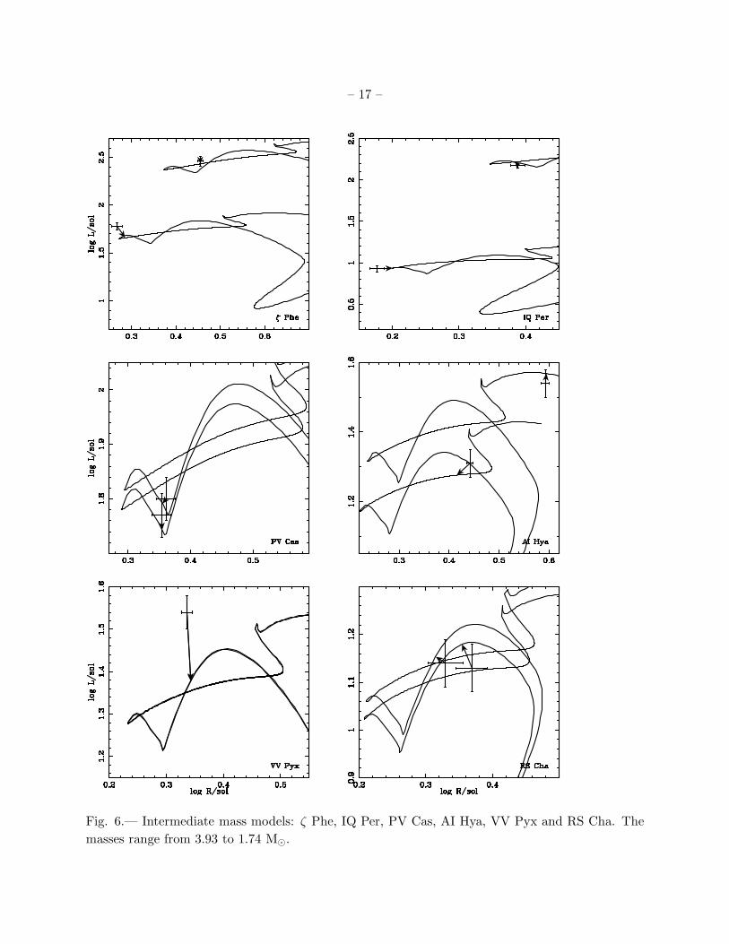
Fig. 6.— Intermediate mass models: ζ Phe, IQ Per, PV Cas, AI Hya, VV Pyx and RS Cha. The

masses range from 3.93 to 1.74 M⊙.

– 18 –

2.3. Intermediate Mass Binaries

Figure 6 shows ζ Phe, IQ Per, PV Cas, AI Hya, VV Pyx, and RS Cha, the group which has

some of the most challenging binaries. The masses range from 3.9 to 1.1 M⊙.

Both ζ Phe and IQ Per have a mass ratio significantly different from one: 0.65 and 0.49

respectively. Because the more massive components will evolve more rapidly, common age is a

stringent constraint. In both cases, the error is dominated by the less massive component. For ζ

Phe, the 2.55 M⊙ secondary is brighter than the model; Pols et al. (1997a) have the same problem.

Ribas et al. (2000) avoid it by using a lower heavy element abundance (0.013) and a higher helium

abundance (0.29). The heavy element abundance might be tested by high resolution spectroscopy.

For IQ Per, the 1.74 M⊙ secondary is too blue; its evolutionary track never gets so hot. Pols et

al. (1997b) attribute the difficulty in fitting ζ Phe and IQ Per to problems in determining Teff

of the secondary (Andersen 1991), which is much dimmer because of the large mass ratios of the

components.

For ζ Phe and IQ Per, it is clear that much of our “difficulty” is due to the relatively small

error bars; see Figure 2. Consequently, small changes may improve the χ2 significantly, even if they

do not correspond to the physics of the system. In the case of IQ Per, use of the Ribas et al. (2000)

value of effective temperature improves the fit, compared to Pols et al. (1997a), as does adjustment

of the abundances.

AI Hydrae is particularly interesting because the primary is fitted by a model which is swiftly

evolving, so that catching it in such a stage is unlikely. Overshoot from the convective core would

broaden the main sequence band and increase the age of the fast evolving primary, allowing the

possibility of a fit with a more probable, slower evolutionary stage. This is consistent with the

conclusions of Pols et al. (1997b), who find that AI Hya is the only binary for which the overshooting

models give a greatly improved fit.

Some of the AI Hya behavior can be attributed to heavy element abundance effects. Both

members are classified as peculiar metal line stars. The heavy element abundance of this system

(from multi-color photometry) is 0.07 (Ribas et al. 2000), which is 3.5 times the value used in the

models. The true interior composition cannot be this metal rich. We have examined a sequence

which had a heavy element abundance of 0.03 rather than 0.02. This modest change gave a dramatic

shift toward lower luminosity (∆ logL ≈ 0.06, which is three times the observational error) and

cooler effective temperatures (∆ log Te ≈ 0.027, which is also three times the observational error).

However, if the heavy element abundance were high only near the surface of the star, the opacity

effects would produce a shift to the red in the evolutionary tracks, which would bring the models

much more in line with the observations.

VV Pyx has almost identical components, so that their coeval origin has almost no effect on

the fit. They track the same path at essentially the same time. The fit is simply the point that the

observational error box is most closely approached, and should be viewed with caution, especially

– 19 –

as the models give a poor fit.

Only PV Cas and RS Cha have good fits (χ2 < 4), and they are pre-main sequence (pre-MS).

RS Cha has previously been suggested to be in a pre-main sequence stage (Mamajek, Lawson &

Feigelson 1999). The pre-MS identification would have important theoretical implications. If true,

it implies that the error in the models occurs after the core convection has been established in these

stars. In any case, convection is an interesting possible cause for the problem; these binaries have

at least one component with convective core burning. PV Cas has sufficiently different masses to

require us to examine the pre-MS fit seriously.

2.4. Is PV Cas Pre-Main Sequence?

Questions have been raised about the evolutionary status of PV Cas since Popper (1987).

Previous attempts to fit the system to main sequence models (Pols et al. 1997a) have been unsat-

isfactory, mainly due to a large and irreconcilable age discrepancy between the members. Fitting

both components to pre-MS models, however, produces excellent agreement.

To test the case for PV Cas being pre-MS, we looked for other observation clues. The double-

lined eclipsing binary system RS Cha was recently found by Mamajek, Lawson & Feigelson (1999,

2000) to be pre-MS. Not only were pre-MS tracks for RS Cha a better fit than post-MS tracks, but

two other observations strengthened the argument: (1) RS Cha had several nearby ROSAT All-Sky

Survey X-ray sources nearby which were found to be very young, low-mass, weak-lined T Tauri

stars, and (2) RS Cha’s proper motion matched that of the T Tauri stars, suggesting a genetic tie.

PV Cas is at a distance of 660 pc (Popper 1987), and a young stellar aggregate or membership

within an OB association could have been previously overlooked.

Searching the Hipparcos and Tycho-2 catalogs, as well as examining PV Cas on the Digitized

Sky Survey, we found no evidence for PV Cas being a member of a known OB Association. More

massive members of a putative association would be included in the Hipparcos catalog with proper

motions similar to that given in the Tycho-2 entry for PV Cas, but none were found. We searched

for known groups of young stars with Vizier at CDS: the compilations of OB Associations by

Ruprecht, Balazs, & White (1982), Melnick & Efremov (1995), and de Zeeuw et al. (1999), and

open clusters by Ruprecht, Balazs, & White (1983) and Lynga (1987). The only possible known

associations that PV Cas could belong to are Cep OB3 (d=840 pc, ∆θ = 4.0◦, vR = −23 km/s)

and Cep OB2 (d=615 pc, ∆θ = 9.5◦, vR = −21 km/s), however their projected separations from

PV Cas are large (600 pc and 100 pc, respectively), and their average radial velocities are far from

Popper’s value for PV Cas (vR = −3 km/s). Hence, PV Cas does not appear to be connected to

any known OB Associations or clusters which help us to infer its nature.

The ROSAT All-Sky Survey (RASS) Bright Source Catalog (BSC; Voges et al. (1999)) and

Faint Source Catalog (FSC; Voges et al. (2000)) were searched to see whether there was any evidence

for a clustering of X-ray-emitting T Tauri stars in the vicinity of PV Cas. No concentration of

– 20 –

sources near PV Cas was detected, although the sensitivity of RASS at 660 pc is about Lx ≃ 1031

erg s−1, corresponding to the very high end of the X-ray luminosity function for T Tauri stars

(Feigelson & Montmerle 1999). Only one RASS-BSC source was within 30 ′ (∼6 pc projected) of

PV Cas, but its fX/fV ratio was 2 magnitudes too high to be a plausible T Tauri star candidate.

The only RASS-FSC source within 30 ′ of PV Cas appeared to be related to a galaxy cluster on

the Digitized Sky Survey.

We conclude that we currently have no evidence for a pre-MS aggregate around PV Cas which

could strengthen the argument for its pre-MS status. However, the Taurus clouds also are forming

low mass pre-MS stars without high mass cluster counterparts.

2.5. Lower Mass Binaries

Figure 7 shows EK Cep, MY Cyg, PV Pup, DM Vir, V1143 Cyg, and UX Men, whose masses

range from 2.03 to 1.12 M⊙. The Ribas et al. (2000) effective temperatures improve the fit for UX

Men.

EK Cep has a large mass ratio. The optimum fit occurs as EK Cep B is still on the pre-MS

track, in agreement with Martin & Rebolo (1993) and Claret, Gimenez, & Martin (1995). We find

that the surface abundance of Li6 is depleted to about 10−4 of its initial value, while Li7 is depleted

from 1.47×10−9 to 0.393×10−9. This corresponds to a depletion of elemental lithium of about 0.57

dex (base 10 logarithm). This is somewhat larger than found by Martin & Rebolo (1993) (0.1 dex),

but may be due to differences in the nuclear reaction rates used. In this range, the depletions are

almost linear in the net cross section for Li7 destruction. A careful analysis with a variety of rates

is warranted: Martin & Rebolo (1993) suggest that the observations are in conflict with pre-MS

models giving a Li depletion greater than 0.3 dex.

Although EK Cep has a large χ2 (χ2 = 10.3) if the radii are used in determining the fitting

function, the situation is different for logL-log Teff , the conventional HR plane. The observational

errors are now larger, and the corresponding χ2 approaches 4. This confirms the importance of

using the radii directly as a discriminant(Andersen 1991).

MY Cyg and UX Men are found to be well into main sequence hydrogen burning. MY Cyg

is underluminous relative to the models. A higher heavy element abundance would remove the

discrepancy; observational tests of this are needed. Pols et al. (1997b) found Z = 0.024 and Ribas

et al. (2000) found Z = 0.039, which are consistent with this suggestion.

PV Pup and V1143 Cyg are on the pre-MS/MS boundary. The fitting procedure chooses the

cusp at which the star settles down to main sequence burning. This cusp shifts with small changes

in abundance, so these fits would benefit from independent measurement of the abundances in these

binaries.

DM Vir has been updated for Latham et al. (1996). Although the changes were small, the new

– 21 –

Fig. 7.— Lower mass models: EK Cep, MY Cyg, PV Pup, DM Vir, V1143 Cyg, and UX Men.

The masses range from 2.03 to 1.12 M⊙.

– 22 –

fit is in the middle of main sequence hydrogen burning instead of pre-MS contraction. The track

lies well within the error bars; the previous data also had χ2 < 4, although a much younger age

estimate. Because the masses are almost equal, the coeval birth requirement has little effect, and

the ages have a corresponding uncertainty.

2.6. Roche Lobes

Observational selection favors binaries with a small separation. In order to determine the true

usefulness of these systems as tests of models of single star evolution it is necessary to know to

what extent these systems are detached (noninteracting), and how far into the past and the future

this condition is satisfied.

In order to answer this question to first order for the systems in our sample, the average Roche

lobe radius for each star was calculated using

RRoche =0.49a

0.6 + q−2/3 ln(1 + q1/3)

where a is the binary separation and q is the mass ratio with the star in question in the numerator

(Lewin, van Paradijs, & van den Heuvel 1995). This average radius was then compared to the

model radii to estimate when each star overflows its Roche lobe. Dynamical evolution of the orbits

was not taken into account. None of the models indicated significant mass transfer prior to the

ages of the models closest to the observed points since early in the pre-Main Sequence evolution.

Four of the binaries in the sample have at least one member which, according to the model

radii, will overflow their Roche lobes when they are between 1.3 and 2 times older than their

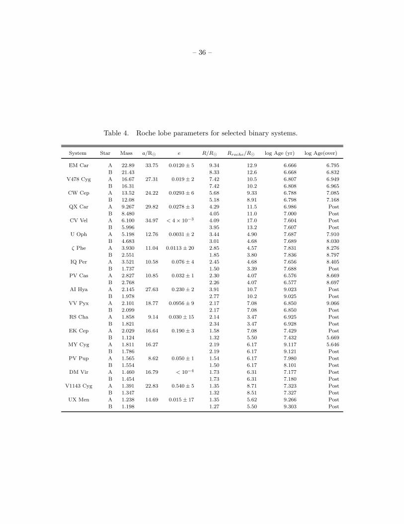
current age. The results of the Roche lobe comparisons are given in Table 4. All stars labeled

“Post” do not exceed their Roche Lobe radius until well into their post-main sequence evolution.

Two stars are in contact early in the pre-main sequence evolution (EK Cep B and MY Cyg A). The

times given for these stars correspond to when they contract below the critical radius and mass

transfer ends. These numbers should be taken as a rough guideline at best, since the dynamical

evolution of protostars is undoubtedly more complex than the simple algorithm used here. The

models corresponding to the primaries EM Car and V478 Cyg exceed their Roche lobe radii in less

than 3× 106 years.

These values are approximate in that dynamical evolution is not taken into account, the model

radii do not match exactly the observed radii, and an approximate Roche lobe geometry was used

to facilitate comparison to the spherically symmetric models.

– 23 –

3. APSIDAL MOTION

Apsidal motion in binaries allows us to infer constraints on the internal mass distributions

(Schwarzschild 1957). Apsidal motion, that is, rotation of the orientation of the orbital ellipse

relative to an inertial frame, does not occur for binary orbits of point particles interacting by New-

tonian gravity. Levi-Civita (1937) showed that the general relativistic expression for the periastron

shift of a double star is the same as for the perihelion shift of Mercury. Following Weinberg (1972)

(see pages 194-7), the shift is

(P/U)GR = 3G(MA +MB)P/a(1 − e2)c2, (2)

where c is the speed of light and G the gravitational constant. Using units of solar masses and

radii, and with the period P in days, this dimensionless number becomes

(P/U)GR = 6.36 × 10−6(MA +MB)P/a(1 − e2), (3)

apsidal orbits per orbit. Tests of general relativity have reached high precision (Will 1998); the

perihelion shift has now been tested to about 3 × 10−3. There has been some controversy as

to a possible breakdown of general relativity because of a discrepancy between observations and

predictions of the apsidal motion of some systems. This has been clarified by Claret (see Claret

(1997, 1998) for a recent discussion), who pointed out errors in theoretical models and difficulties

in observations, especially for systems whose apsidal periods are too long for much to be measured

with modern equipment. We adopt the point of view that general relativity is better tested than

subtleties in the evolution of binary stars, and ascribe errors to other causes (tidal effects not

included, rotational effects, and systematic errors in observational interpretation, for example).

Tides induced by each companion give an additional interaction which is not purely inverse

square in the separation and cause apsidal motion. Quataert, Kumar & On (1996) have discussed

the validity of the classical formula, which we use,

(P/U)CL = (15/a5)[k1R51M2/M1 + k2R

52M1/M2]f(e), (4)

where P is the period of the orbit, U the period of apsidal motion, Mi the mass and Ri the radius

of the star i, and

f(e) = (1 +3

2e2 +

1

8e4)/(1− e2)5, (5)

where e is the eccentricity of the orbit. The separation of the pair in solar radii is

a = 4.207 P23 (M1 +M2)

13 , (6)

if the period P is measured in days and the masses in solar units. The classical apsidal motion

formula gives accurate results when the periods of the low-order quadrupole g, f and p−modes

are smaller than the periastron passage time by a factor of about 10 or more (Quataert, Kumar

& On 1996). For EM Car, the lowest order pulsational mode of the primary has a period of 0.324

– 24 –

days compared with the orbital period of 3.414 days and an eccentricity of 0.0120± 5, so that this

condition is just satisfied.

If we assume that the observed apsidal motion is due only to these two effects, classical simple

tides and general relativity, we have

(P/U)OBS − (P/U)GR = (P/U)CL. (7)

We use the products kiR5i directly for greater precision, but quote the apsidal constants ki for

comparison. Petrova (1995) has pointed out that accuracy problems may exist because the relevant

parameter is kiR5, where ki is the apsidal constant and R is the stellar radius, not just ki alone.

Figure 8 shows the integrand of the apsidal constant, which approaches an asymptotic value

as the integration exceeds about 0.7 of the radius. Inner regions contribute little because of their

small radii; outer regions have little mass. The change from the interior (Henyey) integration to

envelope integration occurs around r/R = 0.5, and is visible in the change in the density of points.

At the join, the temperature is about T ≈ 6× 106 K, and the density ρ ≈ 2.0× 10−2 gcm−3. This

temperature is about ten times the value attained in the early opacity experiments (Perry et al.

1991, 1996) on the NOVA laser, and is about half the goal for the National Ignition Facility (NIF).

For such main sequence (and pre-main sequence) stars, the apsidal constants are most sensitive

to the range of density and temperature which is directly accessed by high energy density laser

experiments (see Remington et al. (1999) and discussion above). In this range, the new opacities

show significant deviation from those previously used in astrophysics (Rogers & Iglesias 1992;

Iglesias & Rogers 1996).

The Petrova & Orlov (1999) catalog contains orbital elements for 128 binaries, including most

(11 of 18) of the binaries in our list. Table 5 gives apsidal constants ki, as well as the observed

and predicted ratios of P/U . Given the significant improvement in the opacities, a critical re-

examination of these data seems warranted.

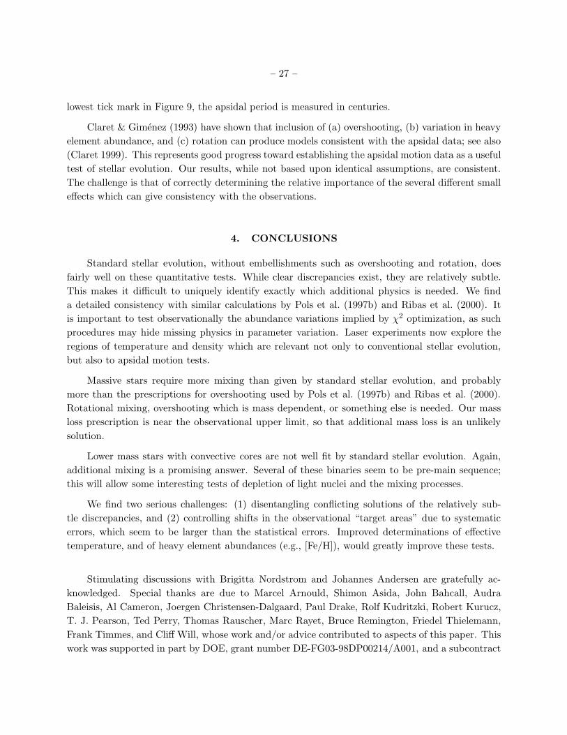
Figure 9 shows the dimensionless rate of apsidal motion, (P/U)CL = (P/U)OBS − (P/U)GR,

which would be due to classical apsidal motion, plotted versus log of half the total binary mass.

P is the orbital period and U the apsidal period. The observational data (corrected for general

relativity) are shown as diamonds, with vertical error bars. The model predictions are shown as

solid squares (χ2 < 4) for the best fits, open triangles for 4 < χ2 < 16, and crosses for χ2 > 16. The

massive binaries with good fits (EM Car, V478 Cyg, and CW Cep; (MA +MB)/2 > 10M⊙) have

predicted apsidal motion in excess of that observed, and QX Car also follows that trend. These

models are not as centrally condensed as the stars. This may be related to the underluminosity

of these models found above. Additional mixing would give more massive, convective cores, which

would result in both greater luminosity and more centrally condensed structure.

Of the lower mass binaries with measured apsidal motion, only PV Cas has a good fit model. Its

predicted apsidal motion is also larger than that observed (the stars are more centrally condensed).

The other binaries need better fitting models before the tests can be convincing. Note that at the

– 25 –

Fig. 8.— Apsidal Constant integrand for EM Car primary.

– 26 –

Fig. 9.— Classical apsidal motion versus mean mass, for our binaries with measured apsidal motion.

(P/U)CL = (P/U)OBS − (P/U)GR is assumed.

– 27 –

lowest tick mark in Figure 9, the apsidal period is measured in centuries.

Claret & Gimenez (1993) have shown that inclusion of (a) overshooting, (b) variation in heavy

element abundance, and (c) rotation can produce models consistent with the apsidal data; see also

(Claret 1999). This represents good progress toward establishing the apsidal motion data as a useful

test of stellar evolution. Our results, while not based upon identical assumptions, are consistent.

The challenge is that of correctly determining the relative importance of the several different small

effects which can give consistency with the observations.

4. CONCLUSIONS

Standard stellar evolution, without embellishments such as overshooting and rotation, does

fairly well on these quantitative tests. While clear discrepancies exist, they are relatively subtle.

This makes it difficult to uniquely identify exactly which additional physics is needed. We find

a detailed consistency with similar calculations by Pols et al. (1997b) and Ribas et al. (2000). It

is important to test observationally the abundance variations implied by χ2 optimization, as such

procedures may hide missing physics in parameter variation. Laser experiments now explore the

regions of temperature and density which are relevant not only to conventional stellar evolution,

but also to apsidal motion tests.

Massive stars require more mixing than given by standard stellar evolution, and probably

more than the prescriptions for overshooting used by Pols et al. (1997b) and Ribas et al. (2000).

Rotational mixing, overshooting which is mass dependent, or something else is needed. Our mass

loss prescription is near the observational upper limit, so that additional mass loss is an unlikely

solution.

Lower mass stars with convective cores are not well fit by standard stellar evolution. Again,

additional mixing is a promising answer. Several of these binaries seem to be pre-main sequence;

this will allow some interesting tests of depletion of light nuclei and the mixing processes.

We find two serious challenges: (1) disentangling conflicting solutions of the relatively sub-

tle discrepancies, and (2) controlling shifts in the observational “target areas” due to systematic

errors, which seem to be larger than the statistical errors. Improved determinations of effective

temperature, and of heavy element abundances (e.g., [Fe/H]), would greatly improve these tests.

Stimulating discussions with Brigitta Nordstrom and Johannes Andersen are gratefully ac-

knowledged. Special thanks are due to Marcel Arnould, Shimon Asida, John Bahcall, Audra

Baleisis, Al Cameron, Joergen Christensen-Dalgaard, Paul Drake, Rolf Kudritzki, Robert Kurucz,

T. J. Pearson, Ted Perry, Thomas Rauscher, Marc Rayet, Bruce Remington, Friedel Thielemann,

Frank Timmes, and Cliff Will, whose work and/or advice contributed to aspects of this paper. This

work was supported in part by DOE, grant number DE-FG03-98DP00214/A001, and a subcontract

– 28 –

from ASCI Flash Center at U. of Chicago.

REFERENCES

Anders, E. & Grevesse, N. 1989, Geochim. Cosmochim. Acta 53, 197

Andersen, J., Nordstrom, B., & Clausen, J. V., 1990, ApJ, 363, 33

Andersen, J. 1991, A&A Rev., 3, 91

Angulo, C., 1999, Nuclear Phys. A 656, 3

Arnett, D. 1996, Supernovae and Nucleosynthesis, Princeton University Press.

Asida, S.M., & Arnett, D. 2000 ApJ, 545, 435

Asida, S., 1998, ApJ, 528, 896

Bahcall, J. N. & Pinsonneault, M. H. 1998, private communication

Bodenheimer, P., 1965 ApJ, 142, 451

Bressan, A., Fagotto, F., Bertelli, G., & Chiosi, C., 1993, A&AS, 100, 647

Canuto, V. M., & Mazzitelli, I., 1991, ApJ, 370, 295

Canuto, V. M., & Mazzitelli, I., 1991, ApJ, 389, 724

Caughlan, G., & Fowler, W. A., 1988, Atomic and Nuclear Data Tables, 40, 283

Christensen-Dalsgaard, J. 2000, private communication

Claret, A., 1995, A&AS, 109, 441

Claret, A., 1997, A&A, 327, 11

Claret, A., 1997, A&AS, 125, 439

Claret, A., 1998, A&A, 330, 533

Claret, A., 1999, A&A, 350, 56

Claret, A., & Gimenez, 1991, A&A, 249, 319

Claret, A., & Gimenez, 1993, A&A, 277, 487

Claret, A., & Gimenez, 1995, A&AS, 114, 549

Claret, A., & Gimenez, 1998, A&AS, 133, 123

– 29 –

Claret, A., Gimenez, & Martin, E. L., 1995, A&A, 302, 741

Dappen, W., & Nayfonov, A., 2000, ApJS, 127, 287

Davidson, S. J., Nazir, K., et al., 2000, J. Quant. Spec. Radiat. Transf., 65, 151

de Jager, C., Nieuwenhiujzen, H., & van der Hucht, K. A. 1988, A&A, 173, 293

de Zeeuw, T., Hoogerwerf, R., de Bruijne, J. H. J., Brown, A. G. a., & Blaauw, A., 1999, AJ, 117,

354

Dominguez, I., Chieffi, A., Limongi, M., & Straniero, O., 1999, ApJ, 524, 226

Elliott, J. R., Miesch, M. S., & Toomre, J., 2000, ApJ, 533, 546

Feigelson, E. D., & Montmerle, T., 1999, ARA&A, 37, 363

Gimenez, A., Clausen, J. V., & Jensen, K. S., 1986, A&A, 159, 157

Guinan, E. F., Ribas, I., Fitzpatrick, E. L., Gimenez, Jordi, C., McCook, G. P., & Popper, D. M.,

2000, ApJ, 544, 404

Henyey, L. G., Wilets, L., Bohm, K. H., LeLevier, Robert, & Levee, R. D., 1959, ApJ, 129, 628

Iglesias, C., Wilson, B. G., et al., 1995 ApJ, 445, 855

Iglesias, C. & Rogers, F. J. 1996 ApJ, 464, 943

Kippenhahn, R., & Wiegert, A., 1990, Stellar Structure and Evolution, Springer-Verlag, Berlin

Kudritzki, R. P., Pauldrach, A., Puls, J., Abbott, & D. C. 1989 A&A, 219, 205

Kurucz, R. L., 1991, in Stellar Atmospheres: Beyond Classical Models, NATO ASI Series C, vol.

341

Latham, D. W., Nordstrom, B., Andersen, J., Torres, G., Stefanik, R. P., Thaller, M., & Bester,

M. J., 1996, A&A, 314, 864

Levi-Civita, T., 1937, Am. J. Math., 59, 225

Lewin, W. H. G., van Paradijs, J., & van den Heuvel, P. J. 1995, X-Ray Binaries, Cambridge

University Press, p.469

Lynga, G., 1987, Catalogue of Open Cluster Data, 5th. ed., Lund Observatory

Maeder, A., 1975, A&A, 40, 303

Martin, E. L., & Rebolo, R., 1993, A&A, 274, 274

Mamajek, E. E., Lawson, W. A., & Feigelson, E. D., 1999, ApJ, 516, L77

– 30 –

Mamajek, E. E., Lawson, W. A., & Feigelson, E. D., 2000, ApJ, 544, 356

Melnick, A. M., & Efremov, Yu. N., 1995, Proc. Astron. Zhurnal, 21, 13

Meynet, G. & Maeder, A., 2000, A&A, 361, 101

Mostovych, A. N., Chan, L. Y., et al., 1995, Phys. Rev. Lett., 75, 1530

Norberg, P., & Maeder, A., 2000, A&A, 359, 1025

Pachoulakis, I., Pfeiffer, R. J., Koch, R. H., & Strickland, D. J., 1996, The Observatory, 116, 89

Perry, T. S., Davidson, S. J., et al., 1991, Phys. Rev. Lett., 67, 3784

Perry, T. S., Springer, P. T., et al., 1996, Phys. Rev. E, 54, 5617

Petrova, A. V., 1995, AZh, 72, 937

Petrova, A. V. & Orlov, V. V., 1999, AJ, 117, 587

Pols, O. R., Tout, C. A., Eggleton, P. P., & Han, Z., 1997, MNRAS, 274, 964

Pols, O. R., Tout, C. A., Schroder, K-P., Eggleton, P. P., & Manners, J., 1997, MNRAS, 289, 869

Popper, D. M., 1987, AJ, 93, 672

Porter, D. H., & Woodward, P. R., 1994, ApJS, 93, 309

Porter, D. H., & Woodward, P. R., 2000, ApJS, 127, 159

Press, W. H., Teukolsky, S. A., Vetterling, W. T., & Flannery, B. P., 1992, Numerical Recipes in

FORTRAN, Second Edition, University Press: Cambridge,

Quataert, E. J., Kumar, P., & On, Chi, 1996, ApJ, 463, 284

Rauscher, T., & Thielemann, K.-F., 2000, Atomic Data Nuclear Data Tables, 75, 1

Remington, B. A., Arnett, D., Drake, R. P., & Takabe, H. 1999, Science, 284, 1488

Ribas, I., Jordi, C., Torra, J., & Gimenez, A., 2000, MNRAS, 313, 99

Rogers, F. J., & Iglesias, C. A., 1992, ApJS, 79, 507

Rosenthal, C. S., Christensen-Dalsgaard, J., Nordlund, Aa., Stein, R. F., & Trampedach, R., 1999,

A&A, 351, 689

Ruprecht, J., Balazs, B., & White, R. E., 1982, Bull. Int. Centre Donnees Stellaires, 22, 132

Ruprecht, J., Balazs, B., & White, R. E., 1983, Soviet Astronomy, 27, 358

– 31 –

Schaller, G., Schaerer, D., Meynet, G., & Maeder, A., 1992, A&AS, 96, 269

Schroder, K-P., Pols, O. R., & Eggleton, P. P., 1997, MNRAS, 285, 696

Schwarzschild, M., 1957, Structure and Evolution of the Stars, Princeton University Press, Prince-

ton, New Jersey, p. 146

Springer, P. T., Fields, D. J., et al., 1992, Phys. Rev. Lett., 69, 3735

Stickland, D. J., Koch, R. H., & Pfeiffer, R. J., 1992, Obs., 112, 277

Stickland, D. J., Lloyd, C., Corcoran, M. F., 1994, Obs., 114, 284

Thielemann, F.-K., Arnould, M., & Truran, J. W., 1988, in Advances in Nuclear Astrophysics,

eds. E. Vangioni-Flam, et al, Editions Frontiers: Gif sur Yvette, and private communication

from FKT

Timmes, F. & Arnett, D., 1999, ApJS, 125, 277

Voges, W., et al., 1999, A&A, 349, 389

Voges, W., et al., 2000, ROSAT All-Sky Survey Faint Source Catalog (RASS-FSC), Max-Planck-

Institut fur Extraterrestriche Physik, Garching

Wasaburo, U., Kiguchi, M., & Kitamura, M. 1994, PASJ, 46, 613

Weinberg, S., 1972, Gravitation and Cosmology, John Wiley & Sons, New York

Will, C. M., 1998, The Confrontation between General Relativity and Experiment: A 1998 Update;

see also www.livingreviews.org/Articles/ for an upcoming review

This preprint was prepared with the AAS LATEX macros v5.0.

– 32 –

Fig. 1.— χ2 for selected binaries.

Fig. 2.— Goodness of fit vectors for selected binaries.

Fig. 3.— Luminosity differences.

Fig. 4.— Radius differences.

Fig. 5.— Massive models.

Fig. 6.— Intermediate mass models.

Fig. 7.— Lower mass models.

Fig. 8.— Apsidal Constant integrand for EM Car primary.

Fig. 9.— Apsidal motion versus mass.

– 33 –

Table 1. Observed parameters for selected binary systems.a

System P(d) Star Spect. Mass/M⊙ Radius/R⊙ log g(cm/s2) log Te(K) logL/L⊙

EM Car 3.41 A O8V 22.3± 0.3b 9.34± 0.17 3.864 ± 0.017b 4.531± 0.026 5.02± 0.10

HD97484 · · · B O8V 20.3± 0.3b 8.33± 0.14 3.905 ± 0.016b 4.531± 0.026 4.92± 0.10

V478 Cyg 2.88 A O9.5V 16.67± 0.45 7.423 ± 0.079 3.919 ± 0.015 4.484± 0.015 4.63± 0.06

HD193611 · · · B O9.5V 16.31± 0.35 7.423 ± 0.079 3.909 ± 0.013 4.485± 0.015 4.63± 0.06

CW Cep 2.73 A B0.5V 12.9± 0.1c 5.685 ± 0.130 4.039 ± 0.024c 4.449± 0.011d 4.26± 0.06e

HD218066 · · · B B0.5V 11.9± 0.1c 5.177 ± 0.129 4.086 ± 0.024c 4.439± 0.011d 4.14± 0.07e

QX Car 4.48 A B2V 9.267± 0.122 4.289 ± 0.091 4.140 ± 0.020 4.395± 0.009d 3.80± 0.04e

HD86118 · · · B B2V 8.480± 0.122 4.051 ± 0.091 4.151 ± 0.021 4.376± 0.010d 3.67± 0.04e

CV Vel 6.89 A B2.5V 6.100± 0.044 4.087 ± 0.036 4.000 ± 0.008 4.254± 0.012d 3.19± 0.05

HD77464 · · · B B2.5V 5.996± 0.035 3.948 ± 0.036 4.023 ± 0.008 4.251± 0.012d 3.15± 0.05

U Oph 1.68 A B5V 5.198± 0.113 3.438 ± 0.044 4.081 ± 0.015 4.211± 0.015d 2.87± 0.08e

HD156247 · · · B B6V 4.683± 0.090 3.005 ± 0.055 4.153 ± 0.018 4.188± 0.015d 2.66± 0.08e

ζ Phe 1.67 A B6V 3.930± 0.045 2.851 ± 0.015 4.122 ± 0.009 4.149± 0.010d 2.46± 0.04e

HD6882 · · · B B8V 2.551± 0.026 1.853 ± 0.023 4.309 ± 0.012 4.072± 0.007d 1.78± 0.04e

IQ Per 1.74 A B8V 3.521± 0.067 2.446 ± 0.026 4.208 ± 0.019 4.111± 0.008d 2.17± 0.03e

HD24909 · · · B A6V 1.737± 0.031 1.503 ± 0.017 4.323 ± 0.013 3.906± 0.008d 0.93± 0.04e

PV Cas 1.75 A B9.5V 2.815± 0.050d 2.297 ± 0.035d 4.165 ± 0.016d 4.032± 0.010d 1.80± 0.04e

HD240208 · · · B B9.5V 2.756± 0.054d 2.257 ± 0.035d 4.171 ± 0.016d 4.027± 0.010d 1.77± 0.04e

AI Hya 8.29 A F2m 2.145± 0.038 3.914 ± 0.031 3.584 ± 0.011 3.851± 0.009d 1.54± 0.02e

+0◦2259 · · · B F0V 1.978± 0.036 2.766 ± 0.017 3.850 ± 0.010 3.869± 0.009d 1.31± 0.02e

VV Pyx 4.60 A A1V 2.101± 0.022 2.167 ± 0.020 4.089 ± 0.009 3.979± 0.009d 1.54± 0.04

HD71581 · · · B A1V 2.099± 0.019 2.167 ± 0.020 4.088 ± 0.009 3.979± 0.009d 1.54± 0.04

RS Cha 1.67 A A8V 1.858± 0.016 2.137 ± 0.055 4.047 ± 0.023 3.883± 0.010d 1.14± 0.05e

HD75747 · · · B A8V 1.821± 0.018 2.338 ± 0.055 3.961 ± 0.021 3.859± 0.010d 1.13± 0.05e

EK Cep 4.43 A A1.5V 2.029± 0.023 1.579 ± 0.007 4.349 ± 0.010 3.954± 0.010 1.17± 0.04

HD206821 · · · B G5Vp 1.124± 0.012 1.320 ± 0.015 4.25 ± 0.010 3.756± 0.015 0.19± 0.07

MY Cyg 4.01 A F0m 1.811± 0.030 2.193 ± 0.050 4.007 ± 0.021 3.850± 0.010d 1.03± 0.04e

HD193637 · · · B F0m 1.786± 0.025 2.193 ± 0.050 4.014 ± 0.021 3.846± 0.010d 1.02± 0.04e

PV Pup 1.66 A A8V 1.565± 0.011 1.542 ± 0.018 4.257 ± 0.010 3.840± 0.019 0.69± 0.08

HD62863 · · · B A8V 1.554± 0.013 1.499 ± 0.018 4.278 ± 0.011 3.841± 0.019 0.67± 0.08

DM Virf 4.67 A F7V 1.454± 0.008 1.763 ± 0.017 4.108 ± 0.009 3.813± 0.007 0.70± 0.03

HD123423f · · · B F7V 1.448± 0.008 1.763 ± 0.017 4.106 ± 0.009 3.813± 0.020 0.70± 0.03

V1143 Cyg 7.64 A F5V 1.391± 0.016 1.346 ± 0.023 4.323 ± 0.016 3.820± 0.007d 0.49± 0.03e

HD185912 · · · B F5V 1.347± 0.013 1.323 ± 0.023 4.324 ± 0.016 3.816± 0.007d 0.46± 0.03e

UX Men 4.18 A F8V 1.238± 0.006 1.347 ± 0.013 4.272 ± 0.009 3.785± 0.007d 0.35± 0.03e

HD37513 · · · B F8V 1.198± 0.007 1.274 ± 0.013 4.306 ± 0.009 3.781± 0.007d 0.29± 0.03e

aDetailed references and discussion may be found in (Andersen 1991).

bStickland, Lloyd, & Corcoran (1994).

cStickland, Koch & Pfeiffer (1992).

dRibas et al. (2000).

eAdjusted here.

fLatham et al. (1996).

– 34 –

Table 2. Parameters for selected binary systems.

System Star Mass logR/R⊙ log Te logL log Age (yr) χ2

EM Car A 22.89 0.972 4.509 4.933 6.666 1.67

HD97484 B 21.43 0.937 4.504 4.843 6.668

V478 Cyg A 16.67 0.879 4.464 4.566 6.807 2.67

HD193611 B 16.31 0.866 4.462 4.530 6.808

CW Cep A 13.52 0.766 4.440 4.245 6.788 2.39

HD218066 B 12.08 0.720 4.421 4.075 6.798

QX Car A 9.267 0.649 4.362 3.698 6.986 11.3

HD86118 B 8.480 0.611 4.343 3.544 7.000

CV Vel A 6.100 0.614 4.231 3.103 7.604 1.30

HD77464 B 5.996 0.603 4.228 3.070 7.607

U Oph A 5.198 0.538 4.198 2.820 7.687 0.43

HD156247 B 4.683 0.480 4.177 2.623 7.699

ζ Phe A 3.930 0.457 4.136 2.409 7.831 11.4

HD6882 B 2.551 0.283 4.028 1.633 7.836

IQ Per A 3.521 0.380 4.119 2.189 7.656 6.92

HD24909 B 1.737 0.195 3.891 0.906 7.688

PV Cas A 2.827 0.362 4.015 1.736 6.576 1.12

HD240208 B 2.768 0.351 4.011 1.698 6.577

AI Hya A 2.145 0.539 3.866 1.494 9.023 21.4

+0◦2259 B 1.978 0.395 3.865 1.204 9.025

VV Pyx A 2.101 0.349 3.920 1.331 6.850 32.2

HD71581 B 2.099 0.350 3.920 1.330 6.850

RS Cha A 1.858 0.324 3.893 1.174 6.925 1.57

HD75747 B 1.821 0.363 3.876 1.183 6.928

EK Cep A 2.029 0.228 3.952 1.217 7.429 10.3

HD206821 B 1.124 0.086 3.761 0.166 7.432

MY Cyg A 1.811 0.347 3.851 1.052 9.117 6.69

HD193637 B 1.786 0.329 3.853 1.025 9.121

PV Pup A 1.565 0.183 3.858 0.750 7.980 1.66

HD62863 B 1.554 0.182 3.855 0.738 8.101

DM Vir A 1.460 0.241 3.802 0.639 7.177 0.15

HD123423 B 1.454 0.240 3.800 0.633 7.180

V1143 Cyg A 1.391 0.169 3.789 0.447 7.323 9.13

HD185912 B 1.347 0.151 3.783 0.388 7.327

UX Men A 1.238 0.140 3.781 0.356 9.266 2.31

HD37513 B 1.198 0.119 3.773 0.283 9.303

– 35 –

Table 3. Predicted instantaneous mass loss rates.

System Star Mass Mass Loss Rate a

EM Car A 22.35 1.82× 10−7

B 20.51 1.17× 10−7

V478 Cyg A 16.78 2.50× 10−8

B 16.47 2.28× 10−8

CW Cep b A 12.87 0.66× 10−8

B 11.88 0.43× 10−8

QX Car A 9.257 1.31× 10−9

B 8.479 6.32× 10−11

aPredicted instantaneous mass loss rate in

M⊙/yr.

bFor IUE upper limit, see Pachoulakis et al.

(1996).

– 36 –

Table 4. Roche lobe parameters for selected binary systems.

System Star Mass a/R⊙ e R/R⊙ Rroche/R⊙ log Age (yr) log Age(over)

EM Car A 22.89 33.75 0.0120 ± 5 9.34 12.9 6.666 6.795

B 21.43 8.33 12.6 6.668 6.832

V478 Cyg A 16.67 27.31 0.019± 2 7.42 10.5 6.807 6.949

B 16.31 7.42 10.2 6.808 6.965

CW Cep A 13.52 24.22 0.0293 ± 6 5.68 9.33 6.788 7.085

B 12.08 5.18 8.91 6.798 7.168

QX Car A 9.267 29.82 0.0278 ± 3 4.29 11.5 6.986 Post

B 8.480 4.05 11.0 7.000 Post

CV Vel A 6.100 34.97 < 4× 10−3 4.09 17.0 7.604 Post

B 5.996 3.95 13.2 7.607 Post

U Oph A 5.198 12.76 0.0031 ± 2 3.44 4.90 7.687 7.910

B 4.683 3.01 4.68 7.689 8.030

ζ Phe A 3.930 11.04 0.0113 ± 20 2.85 4.57 7.831 8.276

B 2.551 1.85 3.80 7.836 8.797

IQ Per A 3.521 10.58 0.076± 4 2.45 4.68 7.656 8.405

B 1.737 1.50 3.39 7.688 Post

PV Cas A 2.827 10.85 0.032± 1 2.30 4.07 6.576 8.669

B 2.768 2.26 4.07 6.577 8.697

AI Hya A 2.145 27.63 0.230± 2 3.91 10.7 9.023 Post

B 1.978 2.77 10.2 9.025 Post

VV Pyx A 2.101 18.77 0.0956 ± 9 2.17 7.08 6.850 9.066

B 2.099 2.17 7.08 6.850 Post

RS Cha A 1.858 9.14 0.030 ± 15 2.14 3.47 6.925 Post

B 1.821 2.34 3.47 6.928 Post

EK Cep A 2.029 16.64 0.190± 3 1.58 7.08 7.429 Post

B 1.124 1.32 5.50 7.432 5.669

MY Cyg A 1.811 16.27 2.19 6.17 9.117 5.646

B 1.786 2.19 6.17 9.121 Post

PV Pup A 1.565 8.62 0.050± 1 1.54 6.17 7.980 Post

B 1.554 1.50 6.17 8.101 Post

DM Vir A 1.460 16.79 < 10−4 1.73 6.31 7.177 Post

B 1.454 1.73 6.31 7.180 Post

V1143 Cyg A 1.391 22.83 0.540± 5 1.35 8.71 7.323 Post

B 1.347 1.32 8.51 7.327 Post

UX Men A 1.238 14.69 0.015 ± 17 1.35 5.62 9.266 Post

B 1.198 1.27 5.50 9.303 Post

– 37 –

Table 5. Apsidal comparisons for selected binary systems.

System Star Mass − log ki (k2R5) a P/UCLb P/UGR

b P/UCL+GRb P/UOBS

b

EM Car A 22.35 2.240 437.9 2.46 0.275 2.74 2.2± 0.3

B 20.51 2.180 290.8

V478 Cyg A 16.78 2.185 169.8 3.21 0.223 3.43 3.0± 0.3

B 16.47 2.175 154.7

CW Cep A 12.87 2.106 52.86 1.61 0.178 1.79 1.640± 0.014

B 11.88 2.090 37.23

QX Car A 9.257 2.122 16.20 0.171 0.170 0.341 0.340± 0.006

B 8.479 2.117 10.96

U Oph A 5.198 2.266 2.721 1.85 0.0827 1.93 2.2± 0.3

B 4.683 2.256 1.549

ζ Phe A 3.930 2.308 0.9756 0.765 0.0624 0.827 1.03± 0.15

B 2.551 2.333 0.1315

IQ Per A 3.521 2.278 0.4619 0.363 0.0553 0.418 0.40± 0.03

B 1.737 2.416 0.0401

PV Cas A 2.815 2.321 0.2647 0.538 0.0572 0.597 0.510± 0.011

B 2.756 2.323 0.2705

VV Pyx A 2.101 2.488 0.1578 0.0215 0.0661 0.0876 0.0039 ± 0.0012

B 2.099 2.488 0.1572

EK Cep A 2.029 2.377 0.05895 0.0153 0.0575 0.0728 0.0030 ± 0.0009

B 1.246 1.867 0.04084

V1143 Cyg A 1.391 2.351 0.02735 0.0106 0.0823 0.0929 0.00195 ± 0.00011

B 1.347 2.288 0.02657

aRadii R in solar units.

bMultiply tabular value by 10−4.

– 38 –

EM Car V478 Cyg CW Cep QX Car CV Vel U Oph

zeta Phe IQ Per PV Cas AI Hya VV Pyx RS Cha

EK Cep MY Cyg PV Pup DM Vir V1143 Cyg UX Men