arX

iv:a

stro

-ph/

0503

713v

1 3

1 M

ar 2

005

Accepted in AJPreprint typeset using LATEX style emulateapj v. 10/09/06

THE C4 CLUSTERING ALGORITHM: CLUSTERS OF GALAXIES IN THE SLOAN DIGITAL SKY SURVEY

Christopher J. Miller,1,2 Robert C. Nichol,3 Daniel Reichart,4 Risa H. Wechsler,5,6 August E. Evrard,7,8

James Annis,9 Timothy A. McKay,7 Neta A. Bahcall,10 Mariangela Bernardi,12 Hans Boehringer,11 Andrew J.Connolly,12 Tomotsugu Goto,13 Alexie Kniazev,17,18,19 Donald Lamb,16 Marc Postman,14 Donald P. Schneider,15

Ravi K. Sheth,12 Wolfgang Voges11

Accepted in AJ

ABSTRACT

We present the “C4 Cluster Catalog”, a new sample of 748 clusters of galaxies identified in thespectroscopic sample of the Second Data Release (DR2) of the Sloan Digital Sky Survey (SDSS). TheC4 cluster–finding algorithm identifies clusters as overdensities in a seven-dimensional position andcolor space, thus minimizing projection effects that have plagued previous optical cluster selection. Thepresent C4 catalog covers ∼ 2600 square degrees of sky and ranges in redshift from z = 0.02 to z = 0.17.The mean cluster membership is 36 galaxies (with redshifts) brighter than r = 17.7, but the catalogincludes a range of systems, from groups containing 10 members to massive clusters with over 200cluster members with redshifts. The catalog provides a large number of measured cluster propertiesincluding sky location, mean redshift, galaxy membership, summed r–band optical luminosity (Lr),velocity dispersion, as well as quantitative measures of substructure and the surrounding large-scaleenvironment. We use new, multi-color mock SDSS galaxy catalogs, empirically constructed fromthe ΛCDM Hubble Volume (HV) Sky Survey output, to investigate the sensitivity of the C4 catalogto the various algorithm parameters (detection threshold, choice of passbands and search aperture),as well as to quantify the purity and completeness of the C4 cluster catalog. These mock catalogsindicate that the C4 catalog is ≃ 90% complete and 95% pure above M200 = 1 × 1014 h−1 M⊙ andwithin 0.03 ≤ z ≤ 0.12. Using the SDSS DR2 data, we show that the C4 algorithm finds 98% ofX-ray identified clusters and 90% of Abell clusters within 0.03 ≤ z ≤ 0.12. Using the mock galaxycatalogs and the full HV dark matter simulations, we show that the Lr of a cluster is a more robustestimator of the halo mass (M200) than the galaxy line-of-sight velocity dispersion or the richness ofthe cluster. However, if we exclude clusters embedded in complex large-scale environments, we findthat the velocity dispersion of the remaining clusters is as good an estimator of M200 as Lr. The finalC4 catalog will contain ≃ 2500 clusters using the full SDSS data set and will represent one of thelargest and most homogeneous samples of local clusters.Subject headings: catalogs, galaxies: clusters: general

1. INTRODUCTION

1 Cerro-Tololo Inter-American Observatory, NOAO, Casilla 603,La Serena, Chile

2 email: cmiller@noao.edu3 Institute of Cosmology and Gravitation, University of

Portsmouth, Portsmouth, PO1 2EG, UK4 Department of Physics and Astronomy, University of North

Carolina, Chapel Hill, NC 275995 Center for Cosmological Physics, Dept. of Astronomy &

Astrophysics, & Enrico Fermi Institute, University of Chicago,Chicago, IL 60637

6 Hubble Fellow7 Department of Physics, University of Michigan, Ann Arbor,

MI 481098 Department of Astronomy, University of Michigan, Ann Ar-

bor, MI 481099 Fermi National Accelerator Laboratory, Batavia, IL 6051010 Princeton University Observatory, Princeton, NJ 0854411 Max-Planck-Institut fur Extraterrestrische Physik, Garching,

Germany12 Department of Physics and Astronomy, University of Pitts-

burgh, PA 1526013 Institute for Cosmic Ray Research, University of Tokyo,

Kashiwanoha, Kashiwa, Chiba 277-0882, Japan14 Space Telescope Science Institute, Baltimore, MD 2121815 Pennsylvania State University, University Park, PA 1680216 University of Chicago, Chicago, IL 6063717 Special Astrophysical Observatory, Nizhnij Arkhyz, Karachai-

Circassia 369167, Russia18 MPA, Knigstuhl 17, 69117 Heidelberg, Germany19 Isaac Newton Institute of Chile, SAO Branch

Catalogs of clusters and groups of galaxies are usedextensively throughout extragalactic astronomy and cos-mology, from constraining the cosmological parameters(e.g., Oukbir & Blanchard 1992; Henry & Arnaud 1991;Viana & Liddle 1996; Bahcall, Fan & Cen 1997; Reichartet al. 1999; Miller et al. 2001a,b), to magnifying themost distant galaxies in the universe (Sand et al. 2002).Considerable effort has been invested over the last half-century in constructing catalogs of clusters and groupsof galaxies (e.g., Zwicky 1952; Abell 1958; Abell et al.1989; Gioia et al. 1990; Lumsden et al. 1992; Dalton etal. 1992; Henry et al. 1995; Postman et al. 1996; Romeret al. 2000; Boehringer et al. 2000; Gladders 2000; Post-man et al. 2002). In this paper, we present one of thefirst catalogs of clusters and groups constructed directlyfrom the spectroscopic data of the Sloan Digital Sky Sur-vey (SDSS). This is now possible because of the presentsize of the SDSS dataset (see Section 7), and is comple-mentary to the SDSS cluster catalogs selected using theSDSS photometric data (e.g., Annis et al. 2000; Goto etal. 2002; Kim et al. 2002; Bahcall et al. 2003; Lee et al.2003).

The distribution of matter in the Universe is describedby the statistics of overdensities. When these overden-sities are small, the equations of motion that follow theevolution of matter can be linearized and solved. As

2 Miller et al.

gravitational clustering is amplified into the non-linearregime, a description of the matter distribution as apoint set of extended dark matter halos becomes moreappropriate (e.g., Cooray & Sheth 2002). How halos arepopulated with galaxies of specific colors and luminosi-ties (typically referred to as the halo occupation) is notknown precisely, and remains a serious challenge in cos-mology and astrophysics. The details of how galaxiesoccupy halos will clearly have an affect on attempts toidentify clusters in optical catalogs. But progress can bemade on both fronts: gaining understanding about howgalaxies populate clusters will be invaluable to those whostudy structure and galaxy formation/evolution. Vice-versa, mock catalogs that are representative of the realUniverse would be invaluable for accurately measuringthe selection function of any clustering algorithm, whichspecifies the contamination and completeness of a datasetand is a prerequisite to many scientific analyses.

The challenge in constructing a cluster catalog fromgalaxy data is to minimize projection effects (or false–positive detections), while maximizing completeness, i.e.controlling the selection function. Previous analyses oflarge optical catalogs of clusters (Lucey et al. 1983;Sutherland 1988; Frenk et al. 1990) have claimed var-ious levels (10-25%) of contamination (see also Miller etal. 1999 and 2002). The next generation of cluster cat-alogs must have very little contamination and preciselyknown selection functions in order to compete with theincreasingly precise cosmological constraints from othermethods (e.g. Perlmutter and Schmidt 2003; Mandolesi,Villa, & Valenziano 2002). Because of concern about thepresence of projection effects in optical cluster catalogs,there has been renewed emphasis over the past decadeon new ways of finding clusters of galaxies in wavebandsother than the optical. For example, many authors haveconstructed catalogs of clusters from X–ray surveys of thesky (Edge & Stewart 1991; Gioia et al. 1990; Boehringeret al. 2000; Romer et al. 2000 among others) as thisis believed to be more robust for selecting mass-limitedsamples than optical methods (see Ebeling et al. 1997).An X-ray selected SDSS cluster sample has also beenpresented by Popesso, Boehringer & Voges (2004). Addi-tionally, many authors have proposed the construction ofcatalogs of clusters using the Sunyaev–Zel’dovich Effect(Carlstrom, Holder & Reese 2002, Romer et al. 2004)and weak gravitational lensing (Wittman et al. 2002).Furthermore, Kochanek et al. (2003) recently presenteda new catalog of clusters derived from the 2MASS infra–red photometric data.

As we outline below, we have now mitigated the prob-lem of projection effects in optical cluster catalogs bysimultaneously using both SDSS photometric and spec-troscopic data to find clusters. The details of our clusterfinding algorithm, which we refer to as the “C4” algo-rithm, are presented in Section 2. The premise of thisalgorithm is that optical clusters and groups of galaxiesare dominated, at their cores, by a single, co–evolvingpopulation of galaxies which possess similar spectral en-ergy distributions, e.g., the “E/S0 ridge-line” or “red en-velope” (Baum 1959; McClure and van den Bergh 1968;Lasker 1970; Visvanathan and Sandage 1977). The ev-idence for such a co–evolving population of galaxies inthe cores of clusters has been presented by many au-thors; see Gladders (2002) for a detailed review of this

evidence. Blakeslee et al. (2003) provide evidence thatthis co–evolving population extends beyond redshift one.As such, Ostrander et al. (1998), Gladders (2000) andGoto et al. (2002) have all used the existence of a co–evolving population of galaxies in the cores of clusters asa basis for their cluster–finding algorithms.

In Figure 1, we present the color–magnitude diagram,in all four of the SDSS colors (u − g, g − r, r − i, i − z),for a newly discovered cluster of galaxies at z = 0.06 inthe SDSS Early Data Release (Stoughton et al. 2002).The nearest cluster in the literature is a Zwicky groupwhich is ∼ 9 arcminutes to the southeast. All galaxiesin this figure are within a projected 1h−1Mpc radius ofthe cluster center (we use h = H0/100 km/s/Mpc). Thefigure demonstrates the existence of a tight relationshipbetween the colors of cluster galaxies, which can have anobserved scatter of ∼ 0.05 (see Bower et al. 1992). Thefigure also illustrates that this “red sequence” of galaxiesis present in all four SDSS colors and not just in theone color system used by Gladders & Yee (2000). Notealso the existence of a “blue ridge-line” in Figure 1 (top-left), which has been highlighted previously by severalauthors (see Chester & Roberts 1964; Tully, Mould, &Aaronson 1982; Baldry et al. 2004). In this one example(at z = 0.06), the 4000 Angstrom break sits betweenthe u and g filters. Thus, the u − g color-magnitudediagram can separate the blue star-forming galaxies fromthe older red passive population. As one moves towardsredder colors, the star-forming and passive populationsbegin to overlap in color. In the reddest colors, the “redsequence” contains a mixture of old passive ellipticals aswell as young star-forming galaxies. So instead of usingan algorithm that attempts to model the “red sequence”,we simply allow for galaxies in clusters to have similarcolors. Our clusters will be detected via a mixture ofgalaxy types, both passively evolving and star-forming.

In this paper, we first present an outline of our algo-rithm based on the premise of galaxies clustering in bothposition and color. We then spend a significant amountof effort analyzing how the C4 algorithm’s free param-eters affect the completeness and contamination of thefinal cluster catalog. We do this using a new breed ofmock galaxy catalogs which populate N-body cosmolog-ical simulations with realistic galaxy populations. Pre-vious authors have realized the necessity of such a de-tailed understanding of their clustering algorithms (e.g.,Diaferio et al. 1999, Adami et al. 2000, Postman etal. 2002, Kim et al. 2002, Goto et al. 2002, and Ekeet al. 2004). In most of these cases, the authors haveembedded fake clusters of various forms into real or sim-ulated data, which are then searched for to characterizethe contamination and completeness of the algorithm. Inthis work, we have gone one step further by using mockgalaxy catalogs generated from full N-body simulations.A similar technique was used in recent work by Eke etal. 2004 on 2dF groups, using N-body simulations pop-ulated with semi-analytic models. The catalogs we use,developed by Wechsler et al (2005), embed galaxies withrealistic luminosities and colors into cosmological simu-lations which contain all of the messiness of structureformation, including merging systems, systems with lotsof substructure, systems with ill-defined E/S0 ridgelines,systems that nearly overlap in redshift space, etc.

In Section 2, we provide details of the C4 algorithm. In

The C4 SDSS Cluster Catalog 3

Fig. 1.— Due to size limitations, this figure only appears in the accepted version or online at www.ctio.noao.edu/ chrism/c4.Color–magnitude relation of galaxies in all four SDSS colors for a previously unknown cluster of galaxies identified in the SDSS DR2 dataset.Black dots are galaxies within a projected aperture of 1h−1Mpc around the cluster center. Red and green dots are cluster members; thered dots have low Hα emission and the green dots have high Hα emission, indicative of ongoing star formation. Error bars on the colorsof the red galaxies indicate the typical color errors in the spectroscopic sample.

4 Miller et al.

Section 3, we describe the use of novel mock catalogs —based on populating large cosmological simulations withrealistic galaxy properties — for calibrating the C4 al-gorithm and determining the completeness and purity ofour SDSS C4 cluster catalog. In Section 5, we introducethe observables that we measure for each cluster, andthen discuss the scaling relations between those observ-ables and halo mass in Section 6. The SDSS data and theSDSS C4 cluster catalog are presented in Section 7 andwe conclude in Section 8. Where appropriate, we haveused h = Ho/100 km s−1 Mpc−1, Ωm = 0.3 and ΩΛ = 0.7throughout this paper.

2. THE C4 ALGORITHM

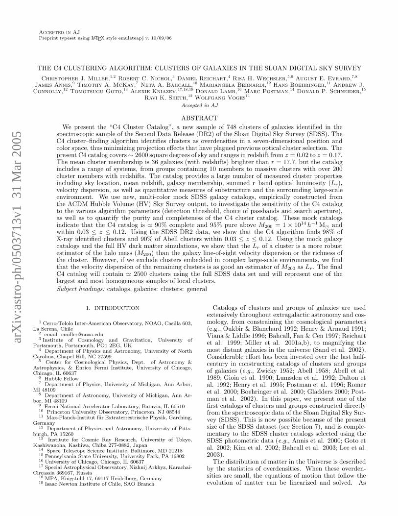
In this section, we present the C4 cluster–finding algo-rithm. Details and tests follow. Many readers will onlywant a brief explanation of the algorithm and we sug-gest they examine the flowchart of the algorithm givenin Figure 2 and read this overview section. For thosewho desire more details, each step is described in moredetail throughout the rest of this section. The applica-tion of the C4 algorithm to the SDSS data is discussedin Section 7.

The C4 algorithm begins by placing each galaxy in aseven dimensional space of right ascension (ra), declina-tion (dec), redshift and four color dimensions (u−g, g−r,r−i, i−z). On each such target galaxy, we then performthe following steps:

1. We place an aperture around each target to onlyinclude galaxies in a specified range of ra, dec, andredshift. We then measure the probability that ev-ery galaxy within this spatial aperture has colorsequal to the target galaxy. The probabilities aresummed to obtain a “number count”.

2. Using the target galaxy’s spatial and color aper-ture, we then select 100 random galaxies and per-form step (1). These 100 random locations pro-vide a “number count” distribution for the targetgalaxy.

3. Using the number count distribution, we computethe probability of obtaining at least the observednumber count around the original target galaxy.By definition, target galaxies with low probabilitieswill be in clustered regions.

4. We repeat this exercise for all (‘target’) galaxiesin our sample and then rank all the target galaxyprobabilities obtained from step 3.

5. Using the false discovery rate algorithm (FDR;Miller et al. 2001c), we determine a thresholdin probability below which target galaxies are re-moved; our threshold choice typically results in theeradication ≃ 90% of all galaxies. The galaxies thatremain are called “C4 galaxies”. By construction,these reside in high density regions with neighborsthat possess similar colors.

6. We determine the local surface density around allC4 galaxies, using only the C4 galaxies, We thenrank order these measured densities and locate C4cluster centers as peaks in this density field.

In summary, the C4 algorithm is a semi-parametricimplementation of adaptive kernel density estimation.The key difference of our approach, compared to pre-vious color-based cluster–finding algorithms, is that wedo not attempt to model either the colors of the clustergalaxies (e.g., Gladders & Yee 2000, Goto et al. 2002)or the properties of clusters (e.g., Kepner et al. 1998;Postman et al. 1996; Kim et al. 2002). Instead, we onlydemand that the colors of nearby galaxies are similar tothose of the target galaxy. In this way we are sensitiveto a diverse range of cluster and group types e.g., ouralgorithm would detect a cluster dominated by a “blue”population of galaxies (see Figure 22).

2.1. Defining the 7-dimensional Search Aperture

Every target galaxy in the dataset has a uniquely de-fined location in a 7-dimensional data–space. For exam-ple, the position of the ith galaxy is defined as:

ri = [rai, deci, zi, mi

u −mig, m

ig −mi

r, mir −mi

i, mii −mi

z],(1)

where miX are the five passband Petrosian magnitudes

from the SDSS PHOTO version 5.4 data reductions (typ-ically abbreviated u, g, r, i, z). No k–corrections are usedherein.

To look for clusters in this 7-dimensional data–space,we need to define a search aperture. Clearly the size ofthis aperture will have an effect on the types of clusterswe find in this data–space. We begin by using a projectedradius that is fixed in comoving coordinates, and specifiesthe ra and dec aperture surrounding the target galaxy.The exact cosmological model used makes little differenceover the redshift range we examine here, (z ∼ 0.1). Thisaperture can be tuned to find the size that optimizescompleteness and purity in the mock galaxy catalogs.

We next define the redshift (or line–of–sight) dimen-sion of the C4 search aperture. For the spectroscopicSDSS sample, all galaxies have known redshifts and wesimply place a z-constraint around the target galaxy. Forthe SDSS photometric sample, one would need estimatedredshifts or else this constraint must be dropped entirely.We have chosen to convert redshift to co-moving distanceunder an assumed model, but one could also simply letthe length of the redshift dimension vary with redshift.

Finally, we must define the color part of our searchaperture. The size of the four color dimensions will bedriven by the well-established intrinsic color-magnituderelation (CMR) seen in clusters (see Figure 1) and theexpected errors on the SDSS magnitudes. The CMR isknown to have a linear relationship with a small nega-tive slope (with increasing magnitude) and small scatter(Bower et al. 1992). Therefore, the size of the “color-box” should be set to capture the full range of colorsin the CMR, from the brightest to the faintest clustergalaxies in any given cluster in our data. We addition-ally include the known statistical (1σ) uncertainties inthe individual galaxy magnitudes. For the SDSS maingalaxy spectroscopic sample, these errors are minimal(less than 0.1% at mr = 17.7). We sum in quadraturethese statistical errors and also a systematic uncertaintyvia:

δCxy =√

σ2xy(stat) + σ2

xy(sys), (2)

The C4 SDSS Cluster Catalog 5

Fig. 2.— Flow chart describing the algorithm

where σ2xy(stat) is the observed error for the two magni-

tudes (x, y), summed in quadrature. Here σ2xy(sys) is a

measure of the inherent scatter in the CMR (see below).Therefore, for each i galaxy the size of the color box isgiven by,

δCi = [δCiug, δC

igr, δC

iri, δC

iiz]. (3)

We have used the Petrosian magnitudes reported bythe SDSS throughout, as it is better suited for the anal-yses of galaxies in the SDSS spectroscopic sample (seeStoughton et al. 2001). However, our final cluster catalogis robust against the use of Petrosian versus model mag-nitudes. We do not apply evolutionary or k–correctionsto our data, as we are looking for galaxies clustered inboth position and color around another galaxy: for agiven redshift and color of a galaxy, any excess of neigh-boring galaxies with similar colors should occur indepen-dent of any evolutionary effects and k–corrections.

Once we have defined the search aperture around a tar-get galaxy, we then “count” the number of neighboringgalaxies within that aperture. To do this, we demand

that any neighboring galaxy fit exactly within the spa-tial part of the aperture (ra, dec, and redshift) as thesedimensions are accurately known.

In the color dimensions, we allow for uncertainties inboth the color box of the target galaxy and the individualcolors of surrounding galaxies. Specifically, we replacethe color boxes with Gaussians having widths specifiedby Equation (4), which “softens” the sides of the 4-dcolor box. We also treat the errors on the individualgalaxies as Gaussians. We then measure the the jointprobability that any galaxy falls within the color box ofthe target galaxy. We then sum these probabilities forall neighboring galaxies and report this as the “numbercount” of neighboring galaxies.

2.2. Building the Count Distributions

The next step in the C4 algorithm is to build a distribu-tion of expected number counts for each target galaxy,given that it was in a random position. We place the7-d aperture of the target galaxy around 100 randomlychosen galaxies and “count” the neighbors as described

6 Miller et al.

above. We allow for the fact that our algorithm canbe run on the SDSS photometric data, in which casethe seeing conditions and galactic extinction can have alarge effect on the selection function of the SDSS pho-tometric sample. The random galaxies can be selectedsuch that they have the same seeing and reddening asthe target galaxy. However, on the complete SDSS spec-troscopic sample, we ignore this constraint. From these100 randomly chosen locations in the data, we constructa distribution of counts for the 7-d aperture of the targetgalaxy. So long as we expect no more than half of thegalaxies to be in clustered environments (i.e., have highercounts with respect to the mean), the medians of thesedistributions are robust descriptors of the distributions.

2.3. Determining Probabilities

By this stage, we have defined a unique aperture for thetarget galaxy. We have measured the number of neigh-boring galaxies within its aperture and built a count dis-tribution from 100 random locations at the same red-shift of the target galaxy. We then ask the question:how likely is the observed neighboring galaxy count giventhe distribution of neighboring galaxy counts for a spec-ified 7-d aperture? The exact form of the distributionof neighboring galaxy counts depends on the number ofcounts measured. For example, in the photometric SDSSdata, where there are millions of galaxies, the distribu-tions of neighboring galaxy counts is Gaussian. However,in the spectroscopic data, the count distributions cansometimes be small and Poissonian. As a compromise,we adopt the Gaussian approximation to the Poisson. Inorder to justify the basis of Poissonian statistics, we needto meet the following requirements in the count distribu-tion; i) the count within an aperture of zero volume iszero, ii) each of the 100 randomly chosen counts mustbe independent, iii) the count values depend only on thesize of the aperture, iv) the aperture size does not changewhen building the count distributions, and v) no twocounts come from the same location. Requirements i,ii,ivand v are already met in our algorithm, while iii requiresthat the randomly selected points have an underlyingcount distribution that is also random. This, of course,is not true for all galaxies, as galaxies are known to clus-ter, and galaxies within clusters have a higher neighborcount than those in the field. However, if a majority ofthe randomly selected galaxies are “field-like”, i.e., lessclustered then the older elliptical population in clustersand groups, then we can expect iii to hold. At worst,this assumption produces a small bias by slightly raisingour probabilities, resulting in a loss of statistical power(which would affect the C4 completeness), and so ourPoisson assumption is a conservative one.

The Gaussian approximation to the Poisson distribu-tion has the convenient feature that the width of theGaussian is equal to the square root of the mean of thePoisson distrubution. Thus, when we build the countdistributions based on the 100 random locations, we onlyneed to calculate the median, which then fully describesthe Gaussian approximation. Thus, the probablility thata target galaxy looks like a field galaxy is determinedsolely from the count around the target and the medianof the counts around the 100 random locations.

2.4. Repeat

Once the above steps are performed on the first targetgalaxy, we then repeat for all galaxies in sample. Thisis conducted in no specific order. Once we have loopedover the entire sample, every galaxy has a probabilitythat it is a “field galaxy”. These probablities are rankedso that a threshold can be applied to separate the clustergalaxies from the field galaxies.

2.5. Choosing a Threshold

Miller et al. (2001c) present a new thresholding tech-nique known as the False Discovery Rate (FDR) origi-nally devised by Benjamini and Hochberg (1995). Thistechnique allows one to choose a statistically meaning-ful threshold, in the sense that the fraction of false pos-itive detections over the total number of detections iscontrolled. We apply the techniques discussed in Milleret al. here. Briefly, this involves choosing a priori themaximum fraction of acceptable false discoveries (α) oneis willing to tolerate. The p-values (probabilities) arerank–listed (from lowest to highest) and a line of slopeα drawn. Where the two lines intersect for the first timedefines the threshold one must use to guarantee the frac-tion of false discoveries (see Miller et al. 2001c and Hop-kins et al. 2002 for some examples). After applyingthe FDR technique, all galaxies above the threshold arecalled “cluster-like” or “C4” galaxies and are then usedto identify C4 cluster centers.

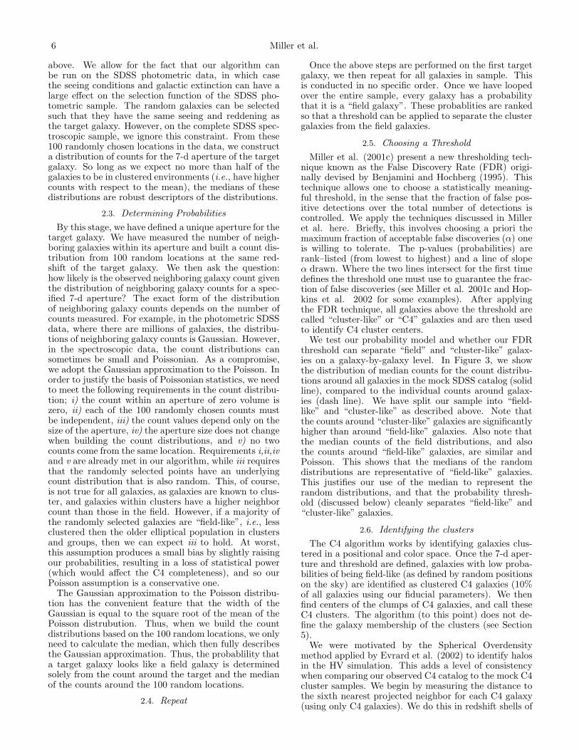
We test our probability model and whether our FDRthreshold can separate “field” and “cluster-like” galax-ies on a galaxy-by-galaxy level. In Figure 3, we showthe distribution of median counts for the count distribu-tions around all galaxies in the mock SDSS catalog (solidline), compared to the individual counts around galax-ies (dash line). We have split our sample into “field-like” and “cluster-like” as described above. Note thatthe counts around “cluster-like” galaxies are significantlyhigher than around “field-like” galaxies. Also note thatthe median counts of the field distributions, and alsothe counts around “field-like” galaxies, are similar andPoisson. This shows that the medians of the randomdistributions are representative of “field-like” galaxies.This justifies our use of the median to represent therandom distributions, and that the probability thresh-old (discussed below) cleanly separates “field-like” and“cluster-like” galaxies.

2.6. Identifying the clusters

The C4 algorithm works by identifying galaxies clus-tered in a positional and color space. Once the 7-d aper-ture and threshold are defined, galaxies with low proba-bilities of being field-like (as defined by random positionson the sky) are identified as clustered C4 galaxies (10%of all galaxies using our fiducial parameters). We thenfind centers of the clumps of C4 galaxies, and call theseC4 clusters. The algorithm (to this point) does not de-fine the galaxy membership of the clusters (see Section5).

We were motivated by the Spherical Overdensitymethod applied by Evrard et al. (2002) to identify halosin the HV simulation. This adds a level of consistencywhen comparing our observed C4 catalog to the mock C4cluster samples. We begin by measuring the distance tothe sixth nearest projected neighbor for each C4 galaxy(using only C4 galaxies). We do this in redshift shells of

The C4 SDSS Cluster Catalog 7

Fig. 3.— We show the counts from the field based on the median of 100 random locations for each galaxy (solid) and counts aroundeach specific galaxy (dotted). On the left we show for “field-like” galaxies, while on the right we show “cluster-like” galaxies. Notice that“cluster-like” galaxies have more neighbors than the median of the field.

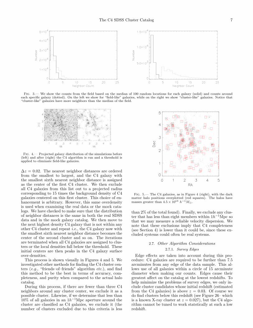
Fig. 4.— Projected galaxy distribution of the simulations before(left) and after (right) the C4 algorithm is run and a threshold isapplied to eliminate field-like galaxies.

∆z = 0.02. The nearest neighbor distances are orderedfrom the smallest to largest, and the C4 galaxy withthe smallest sixth nearest neighbor distance is assignedas the center of the first C4 cluster. We then excludeall C4 galaxies from this list out to a projected radiuscorresponding to 15 times the background density of C4galaxies centered on this first cluster. This choice of en-hancement is arbitrary. However, this same overdensityis used when examining the real data or the mock cata-logs. We have checked to make sure that the distributionof neighbor distances is the same in both the real SDSSdata and in the mock galaxy catalog. We then move tothe next highest density C4 galaxy that is not within anyother C4 cluster and repeat i.e., the C4 galaxy now withthe smallest sixth nearest neighbor distance becomes thecenter of the second cluster and so on. The iterationsare terminated when all C4 galaxies are assigned to clus-ters or the local densities fall below the threshold. Theseinitial centers are then peaks in the C4 galaxy surfaceover-densities.

This process is shown visually in Figures 4 and 5. Weinvestigated other methods for finding the C4 cluster cen-ters (e.g., “friends–of–friends” algorithm etc.), and findthis method to be the best in terms of accuracy, com-pleteness, and purity when compared to the actual halocatalog.

During this process, if there are fewer than three C4neighbors around any cluster center, we exclude it as apossible cluster. Likewise, if we determine that less than10% of all galaxies in an 1h−1Mpc aperture around thecluster are classified as C4 galaxies, we exclude it (thenumber of clusters excluded due to this criteria is less

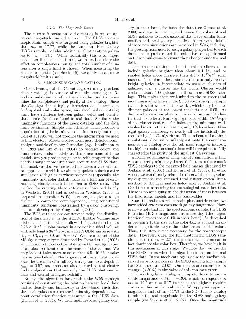
Fig. 5.— The C4 galaxies, as in Figure 4 (right), with the darkmatter halo positions overplotted (red squares). The halos havemasses greater than 4.5 × 1013 h−1M⊙.

than 2% of the total found). Finally, we exclude any clus-ter that has less than eight members within 1h−1Mpc sothat we may measure a reliable velocity dispersion. Wenote that these exclusions imply that C4 completeness(see Section 4) is lower than it could be, since these ex-cluded systems could often be real systems.

2.7. Other Algorithm Considerations

2.7.1. Survey Edges

Edge effects are taken into account during this pro-cedure: C4 galaxies are required to be further than 7.5arcminutes from any edge of the data sample. This al-lows use of all galaxies within a circle of 15 arcminutediameter when making our counts. Edges cause theirgreatest affect on the catalog at the lowest redshifts. Tohelp minimize the problems of survey edges, we only in-clude cluster candidates whose initial redshift (estimatedfrom the C4 galaxies) is above z = 0.03. Of course wedo find clusters below this redshift (see Figure 26– whichis a known X-ray cluster at z = 0.027), but the C4 algo-rithm cannot be tuned to work statstically at such a lowredshift.

8 Miller et al.

2.7.2. The Magnitude Limit

The current incarnation of the catalog is run on ap-parent magnitude limited surveys. The SDSS spectro-scopic Main sample was targeted using galaxies brighterthan mr = 17.77, while the Luminous Red Galaxy(LRG) sample includes additional elliptical-type galax-ies to mr = 19.5. While technically this is an inputparameter that could be tuned, we instead consider theeffect on completeness, purity, and total number of clus-ters after a single limit is chosen. When measuring thecluster properties (see Section 5), we apply an absolutemagnitude limit as well.

3. A MOCK SDSS GALAXY CATALOG

One advantage of the C4 catalog over many previouscluster catalogs is our use of realistic cosmological N-body simulations to refine the algorithm and to deter-mine the completeness and purity of the catalog. Sincethe C4 algorithm is highly dependent on clustering inboth spatial and color space, any mock galaxy catalogmust have relations between galaxy color and densitythat mimic the those found in real data. Similarly, theluminosity functions of the mock catalogs and the datamust be similar. Simple bias schemes which produce apopulation of galaxies above some luminosity cut (e.g.,Cole et al 1998) will not produce the information we needto find clusters. Mocks created from more detailed semi-analytic models of galaxy formation (e.g., Kauffmann etal. 1999 and Eke et al. 2004) do produce colors andluminosities; unfortunately at this stage none of thesemodels are yet producing galaxies with properties thatnearly enough reproduce those seen in the SDSS data.The mock catalog we use here thus takes a very empiri-cal approach, in which we aim to populate a dark mattersimulation with galaxies whose properties (especially, theluminosity and color distributions as a function of envi-ronment) closely match those seen in SDSS data. Themethod for creating these catalogs is described brieflyin Wechsler (2004) and in detail in Wechsler (2005, inpreparation, hereafter W05); here we just give a roughoutline. A complementary approach, using conditionalluminosity functions constrained by galaxy clustering,has been developed by Yang et al. (2004).

The W05 catalogs are constructed using the distribu-tion of dark matter in the ΛCDM Hubble Volume sim-ulation. The simulation follows 109 particles of mass2.25× 1012h−1 solar masses in a periodic cubical volumewith side length 3h−1Gpc, in a flat Λ CDM universe withΩm = 0.3, σ8 = 0.9, and h = 0.7. We use a subset of theMS sky survey output described by Evrard et al. (2002)which mimics the collection of data on the past light coneof an observer located at the center of the volume. Weonly look at halos more massive than 4.5×1013h−1 solarmasses (see below). The large size of the simulation al-lows the creation of a full-sky survey out to a depth ofzmax = 0.57, and thus can also be used to test clusterfinding algorithms that use only the SDSS photometricdata and extend to higher redshift.

Briefly, the algorithm for creating the W05 catalogsconsists of constraining the relation between local darkmatter density and luminosity in the r-band, such thatthe mock galaxies match the luminosity-dependent two-point correlation function measured in the SDSS data(Zehavi et al. 2004). We then measure local galaxy den-

sity in the r-band, for both the data (see Gomez et al.2003) and the simulation, and assign the colors of realSDSS galaxies to mock galaxies that have similar lumi-nosities and local galaxy densities. All relevant detailsof these new simulations are presented in W05, includingthe prescriptions used to assign galaxy properties to eachdark matter particle and the extensive tests performedon these simulations to ensure they closely mimic the realdata.

The mass resolution of the simulation allows us toinclude galaxies brighter than about 0.4 L⋆, and toresolve halos more massive than 4.5 × 1013h−1 solarmasses. Therefore, these simulations can only resolvebright galaxies in intermediate–to–massive clusters ofgalaxies, e.g., a cluster like the Coma Cluster wouldcontain about 500 galaxies in these mock SDSS cata-logs. This makes them well-suited to the brighter (andmore massive) galaxies in the SDSS spectroscopic sample(which is what we use in this work), which only includesdimmer galaxies at the lowest redshifts z < 0.05. Asdiscussed above, we place a constraint on any C4 clus-ter that there be at least eight galaxies within 1h−1Mpcof the cluster centers. For halos at the minimum well-resolved mass in the simulation, only 1% have fewer thaneight galaxy members, so nearly all are intrisically de-tectable by the C4 algorithm. This indicates that thesesimulations allow us to reliably estimate the complete-ness of our catalog over the full mass range of interest,but higher resolution simulations will be required to fullycharacterize the purity of the smallest C4 systems.

Another advantage of using the HV simulation is thatwe can directly relate any detected clusters in these mockSDSS catalogs to the measured halo masses discussed byJenkins et al. (2001) and Evrard et al. (2002). In otherwords, we can directly relate the observables (e.g., veloc-ity dispersions and summed total cluster optical lumi-nosities) to the dark matter halos used by Jenkins et al.(2001) for constructing the cosmological mass function.There is no ambiguity in the definition of mass betweenthe theoretical models and the observables.

Since the real data will contain photometric errors, wehave added errors to each mock galaxy magnitude. How-ever, we note that for the spectroscopic sample, the SDSSPetrosian (1976) magnitude errors are tiny (the largestfractional errors are < 0.1% in the r-band). As describedin Section 2.1, the size of the color-box is at least an or-der of magnitude larger than the errors on the colors.Thus, this step is not necessary for the spectroscopicdata. However, when the full photometric SDSS sam-ple is used (to mr = 22), the photometric errors can infact dominate the color-box. Therefore, we have built inthis mechanism at this stage. We note that we use thetrue SDSS errors when the algorithm is run on the realSDSS data. In the mock catalogs, we use the median ob-served error for galaxies in the SDSS main galaxy sample(see Strauss et al. 2002). Our results are insensitive tochanges (<50%) in the value of this constant error.

The mock galaxy catalog is complete down to an ab-solute magnitude of Mr = −19.6, which corresponds tomr = 19.2 at z = 0.17 (which is the highest redshiftcluster we find in the real data). We apply an apparentmagnitude limit of mr ≤ 17.7 to the SDSS mock catalogto mimic the real magnitude–limited SDSS main galaxysample (see Strauss et al. 2002). Once the magnitude

The C4 SDSS Cluster Catalog 9

limit is applied and the errors are added, we are able torun the exact same C4 algorithm on the mock galaxycatalogs and identify clusters as outlined in Section 2.For this work, we have used a volume that is larger andmore contiguous than the SDSS DR2. However, edge ef-fects are handled identically in the data as they are inthe mock catalogs (see Section 2.7.1). While we havenot applied the SDSS targeting algorithm, in Section 7.1we study this issue in detail and find that the effect oncompleteness and purity is small.

4. COMPLETENESS, PURITY, AND TUNING THE C4ALGORITHM

We use the SDSS mock galaxy catalogs to test the C4algorithm, fine tune the choice of parameters, and mea-sure the completeness and purity of the catalog (i.e., theselection function). We do this by running the C4 algo-rithm on the mock galaxy catalog, and comparing thefound C4 clusters to the known halos from Evrard et al.(2002). To make the comparison, we apply a matchingalgorithm to associate C4 clusters with halos. We haveinvestigated several prescriptions for matching these twodatasets and have found that our matches are robustagainst the details of the matching algorithm. Here, wepresent results based on matching a dark matter halowith any C4 cluster within a projected distance corre-sponding to one virial radius and within ∆z = 0.005.We discuss this matching in more detail in Section 4.2.To estimate purity, we match clusters to any simulatedhalo within the estimated r200 of the “observed” C4 clus-ter, while for the completeness measurements we matcheach “observed” C4 cluster to the nearest dark matterhalo within ∆z = 0.005 and the projected r200 of thehalo.

This method for matching allows for multiple matches.In other words, when measuring completeness, multipleC4 clusters can be matched to one HV halo, and similarlywhen measuring purity, multiple halos can be matchedto a single C4 cluster. There are many ways to deal withthis problem. For instance, when multiple halos matchto one C4 cluster, we could take the most massive haloas the fiducial match. Or we could take the halo thathas the most similar luminosity to the C4 cluster, orany other method. We have chosen to simply take thematch that is closest in separation on the sky (and within∆z = 0.005). We have investigated a few of the othermethods we mentioned and find no clear winner. The C4algorithm finds fewer clusters in the mock catalog thanthere are real HV halos (i.e., the C4 algorithm is never100% complete). As seen and discussed in the followingsections, this completeness drops with halo mass suchthat the C4 algorithm can miss up to 50% of the halosat masses ∼ 5 × 1013h−1 solar masses. This means thatthere will always be more multiple halo matches to theC4 clusters than vice versa. On average, 50% of the C4clusters have multiple halos within ∆z = 0.005 and r200

while only 5% of halos have multiple C4 clusters withinthose same constraints.

After the matching is done, we will plot the cumulativequantity:

Purity(Lr) =Number(> Lr) C4 Matched to Halos

Number(> Lr) C4 Clusters Found(4)

Completeness(M200) =Num(> M200) Halos Matched to C4

Num(> M200) Total Halos(5)

where M200 is the mass within a radius that is 200 timesthe critical density and Lr is the summed luminosities ofthe cluster member galaxies as defined in detail in Sec-tion 5. Since completeness is defined against the “true”halos from the mocks, we plot completeness versus halomass. On the other hand, purity is measured from thepoint of view of the measured clustered catalog, and sopurity is plotted against the observable: optical luminos-ity. It is important to keep in mind that the high mass(or high luminosity) systems are rare, and so the purityand completeness measurements can be noisy in theseregimes.

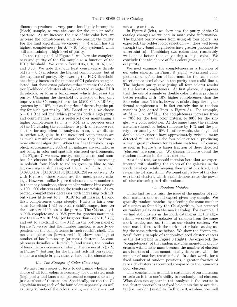
In Figure 6 (left), we present the completeness andpurity of the mock C4 catalog as a function of differ-ent radii for the search aperture: 500, 1000, 2000, and6000h−1kpc. In this figure, the other dimensions of thesearch aperture are fixed at the final values as discussedbelow. A radius of 500h−1kpc (black) appears to be toosmall, as it significantly lowers the completeness of oursample for all but the most massive systems (although itdoes produce the purest sample). However, larger search-radii make little difference to the completeness or purityof the algorithm. The highest completeness and purityoccur when a co-moving radius of 1h−1Mpc is used (thered line).

We varied the redshift dimension of the 7-d box to bea co-moving length of 25, 50, 100, 200h−1Mpc. The sizeof the aperture in the redshift direction must be largeenough to allow for significant (and unknown) peculiarvelocities of galaxies within massive clusters of galax-ies and therefore, our 3-dimensional positional apertureis shaped like a narrow cylinder. Using these tests, wefind that our final cluster catalog is independent of thelength of the line-of-sight aperture. We attribute this tothe fact that there are not many clusters or groups thatlie directly along the line-of-sight that also have similarglobal colors. Alternatively, one could argue that by notusing k–corrections for our SDSS colors, we have alreadyaccounted for the redshift dimension in the “color-box”.We set the redshift dimension of the search aperture to50h−1Mpc.

In the middle panel of Figure 6, we show the complete-ness and purity for the mock SDSS catalog as a functionof the “color-box” size, holding constant the spatial partof the search aperture. We examine only the effect ofchanging σxy(sys), using σug(sys) = γ×0.15, σgr(sys) =γ × 0.12, σri(sys) = γ × 0.1, and σiz(sys) = γ × 0.1.These values represent reasonable widths for the color-magnitude relation, decrease with increasing wavelength(as indicated in Figure 1), and are motivated by the re-sults of Goto et al. (2002). However, we note that our al-gorithm is not attempting to model the color-magnituderelation. Thus, we allow the color-box size to be a freeparameter in our algorithm by varying γ as 1, 2, 4, 6. Wethen use the mock galaxy catalogs to tune this variable.We note that the median of σxy(stat) = 0.02 for ourdata changes very little over our magnitude-range (re-call, these are the bright galaxies in the spectroscopicSDSS data). Thus, σxy(sys) is the dominant term inEquation (4).

As seen in Figure 6 (middle), the smallest “color-box”

10 Miller et al.

1011 1012

0.7

0.8

0.9

1.0

Puri

ty (

<L

)

1011 1012

r−band Luminosity (solar)1011 1012

Radius Color Threshold

1014 1015

0.2

0.4

0.6

0.8

1.0

Com

plet

enes

s (>

M)

1014 1015

Halo Mass (M200 solar)1014 1015

Radius Color Threshold

1011 10121

10

100

1000

N (

>L)

1011 1012

r−band Luminosity (solar)1011 1012

Radius Color Threshold

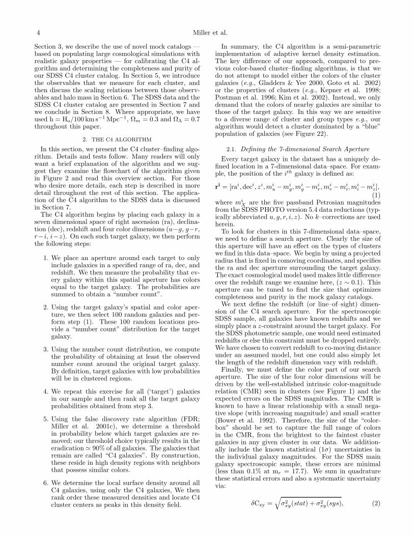
Fig. 6.— How the choice of box size, threshold, and redshift-bin affect completeness and purity for clusters found using the simulatedmock galaxy data. Also show the cumulative number plot (N(> L)) for the mock catalog clusters. The variation of the box size is describedin Section 2.1; the variation of the FDR threshold is described in Section 2.5. Generally, the size of the box increases from black to red togreen to blue. The purity and cumulative number counts are measured against the summed r-band luminosity of the discovered clusters,while the completeness is against the halo mass.

The C4 SDSS Cluster Catalog 11

dimension produces a very pure, but highly incomplete(black) sample, as was the case for the smaller radialaperture. As we increase the size of the color box, weincrease the completeness, while decreasing the purity.For the final algorithm, we choose γ = 4 which has thehighest completeness (for M ≥ 1014 M⊙ systems), whilestill maintaining a high level of purity.

In the right panel of Figure 6, we show the complete-ness and purity of the C4 sample as a function of theFDR threshold. We vary α from 0.05, 0.10, 0.15, 0.20,and 0.50. We note that our least conservative thresh-old (α = 0.5) produces the highest completeness, but atthe expense of purity. By lowering the FDR threshold,one simply increases the number of C4 galaxies being se-lected, but these extra galaxies either increase the detec-tion likelihood of clusters already detected at higher FDRthresholds, or form a background which decreases thepurity. Changing the threshold by a factor of four onlyimproves the C4 completeness for M200 ≤ 1 × 1014M⊙

systems by ∼ 10%, but at the price of decreasing the pu-rity for such systems by 10%. Based on this, we chooseα = 0.1 (the red line) which provides both a high purityand completeness. This is preferred over maintaining ahigher completeness (e.g. α = 0.5), as it provides usersof the C4 catalog the confidence to pick and choose realclusters for any scientific analyses. Also, as we discussin section 4.2, gains in the measured completeness areas much a result of random matches as they are from amore efficient algorithm. When this final threshold is ap-plied, approximately 90% of all galaxies are excluded asnot being in color and spatially clustered environments.

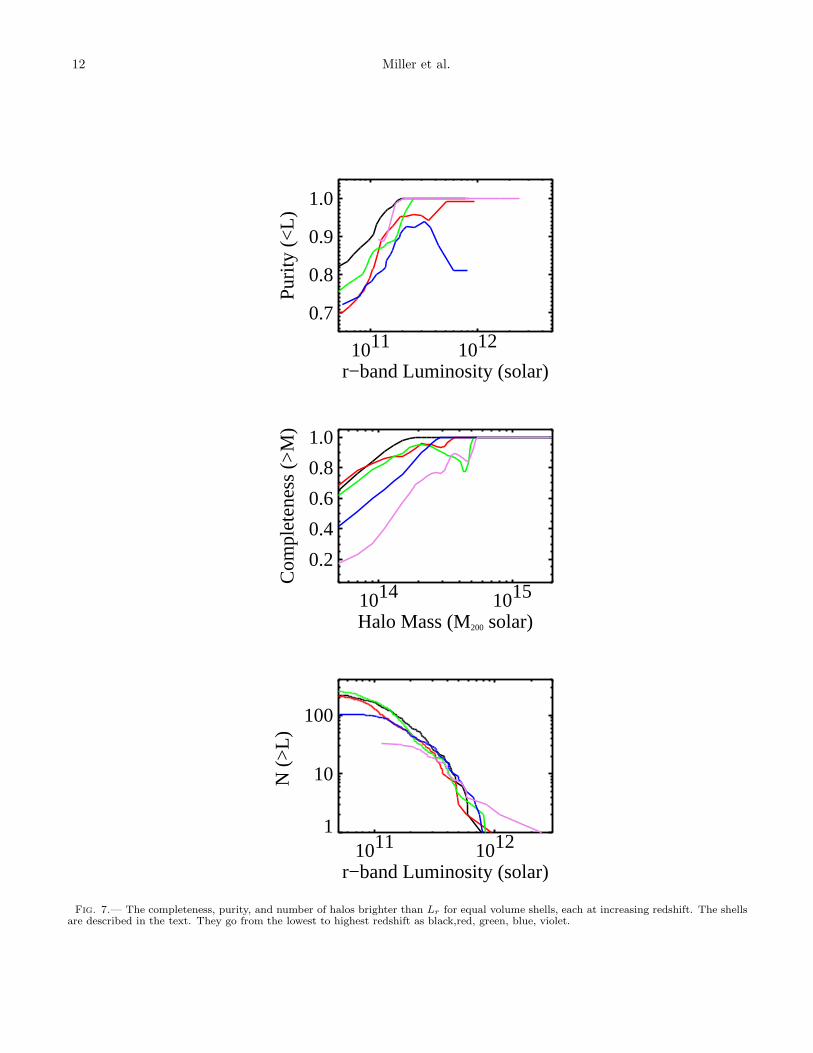
In Figure 7, we show purity, completeness, and num-ber for clusters in shells of equal volume, increasingin redshift from black to red to green to blue to vio-let, covering redshift ranges of [0.03,0.075], [0.075,0.093],[0.093,0.107], [0.107,0.118], [0.118,0.128] respectively. Aswith Figure 6, these panels use the mock galaxy cata-logs. However, unlike Figure 6 whose clusters numberedin the many hundreds, these smaller volume bins contain∼ 100−200 clusters and so the results are noisier. As ex-pected, completeness decreases with increasing redshift,but varies little out to z = 0.107 for all masses. Beyondthat, completeness drops steeply. Purity is fairly con-stant (to within 10%) over all redshift ranges, howeverthe lowest redshift bin is the purest. The C4 catalog is> 90% complete and > 95% pure for systems more mas-sive than ∼ 2× 1014M⊙ (or brighter than ∼ 3× 1011L⊙)and out to a redshift of z ∼ 0.12. In the bottom panel ofFigure 7, we see that the number function is mostly de-pendent on the completeness in each redshift shell. Themost complete bin (lowest redshift) shows the highestnumber of low luminosity (or mass) clusters. As com-pleteness dwindles with redshift (and mass), the numberof found halos decreases similarly. The excess of N(> L)in Figure 7 (bottom) for the highest redshift bin (violet)is due to a single bright, massive halo in the simulations.

4.1. The Strength of Color Clustering

We have run a series of tests to determine whether ourchoice of all four colors is necessary for our stated goals(high purity and known completeness) compared to usingjust a subset of these colors. Specifically, we ran the C4algorithm using each of the four colors separately, as wellas using subsets of the colors, e.g., g − r and r − i, but

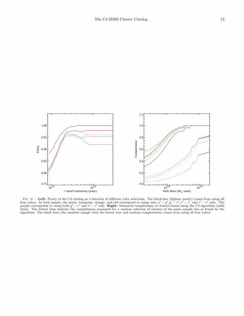
not u − g or i − z.In Figure 8 (left), we show how the purity of the C4

catalog changes as we add in more color information.The highest purity comes from using all four colors. Asexpected, the reddest color selection i−z does well (eventhough the z-band magnitudes have greater photometricuncertainties). Combining two colors does reasonablywell and is better than only using a single color. Weconclude that the choice of four colors gives us our high-est purity.

We next examine the completeness as a function ofour color choices. In Figure 8 (right), we present com-pleteness as a function of halo mass for the same colorselections as used above in the purity case (solid lines).The highest purity case (using all four colors) resultsin the lowest completeness. At first glance, it appearsthat the use of a single or double color criteria producesbetter results, with 10% higher completeness than thefour color case. This is, however, misleading: the higherformal completeness is in fact entirely due to randommatches (the dotted lines in Figure 8). For example,at M = 1 × 1014 M⊙, the completeness increases from∼ 70% for the four color criteria to 80% for the sin-gle i − z color selection. At the same time, the randommatches (described below) increase by 10% and the pu-rity decreases by ∼ 10%. In other words, the single anddouble color criteria have approximately twice as manydetected “clusters” as the four color criteria, producinga much greater chance for random matches. Of course,as seen in Figure 8, a larger fraction of these detected“clusters” are spurious. We discuss in more detail therandom matches in the next section.

As a final test, we should mention here that we exper-imented with shuffling the colors of the galaxies in themock catalogs, while keeping their positions fixed, andre-ran the C4 algorithm. We found only a few of the clos-est richest clusters, which again demonstrates the powerof color clustering in 4–dimensions.

4.2. Random Matches

These first results raise the issue of the number of ran-dom matches one would expect given any sample. Wequantify random matches by selecting the same numberof clusters as found by the C4 algorithm, but centeredon random galaxies in the mock catalog. For example, ifwe find 934 clusters in the mock catalog using the algo-rithm, we select 934 galaxies at random from the samemock catalog and use them as our cluster centers. Wethen match these with the dark matter halo catalog us-ing the same criteria as before. We show the “complete-ness” from a sample of randomly-placed cluster centersas the dotted line in Figure 8 (right). As expected, the“completeness” of the random matches monotonically in-creases with cluster mass because the number of clustersas a function of mass monotonically decreases, while thenumber of matches remains fixed. In other words, for afixed number of random positions, a greater fraction ofrare rich clusters is recovered compared to the numerouspoor clusters.

This conclusion is as much a statement of our matchingcriteria as it is to one’s ability to randomly find clusters.What does not appear in this analysis is the scatter inthe cluster observables at fixed halo mass due to acciden-tal (i.e. random) matches. In Figure 9, we show how well

12 Miller et al.

1011 1012

r−band Luminosity (solar)

0.7

0.8

0.9

1.0

Pur

ity (

<L)

1014 1015

Halo Mass (M200 solar)

0.2

0.4

0.6

0.8

1.0

Com

plet

enes

s (>

M)

1011 1012

r−band Luminosity (solar)

1

10

100

N (

>L)

Fig. 7.— The completeness, purity, and number of halos brighter than Lr for equal volume shells, each at increasing redshift. The shellsare described in the text. They go from the lowest to highest redshift as black,red, green, blue, violet.

The C4 SDSS Cluster Catalog 13

1011 1012

r−band Luminosity (solar)

0.75

0.80

0.85

0.90

0.95

1.00

Pur

ity

1014 1015

Halo Mass (M200 solar)

0.0

0.2

0.4

0.6

0.8

1.0

1.2

Com

plet

enes

s

Fig. 8.— Left: Purity of the C4 catalog as a function of different color selections. The black-line (highest purity) comes from using allfour colors. In both panels, the green, turquoise, orange, and red correspond to using only u′

− g′, g′ − r′, r′ − i′, and i′ − z′ only. Thepurple corresponds to using both g′ − r′ and r′ − i′ only. Right: Measured completeness of clusters found using the C4 algorithm (solidlines). The dotted lines indicate the completeness measured for a random selection of clusters of the same sample size as found by thealgorithm. The black lines (the smallest sample with the lowest true and random completeness) comes from using all four colors.

14 Miller et al.

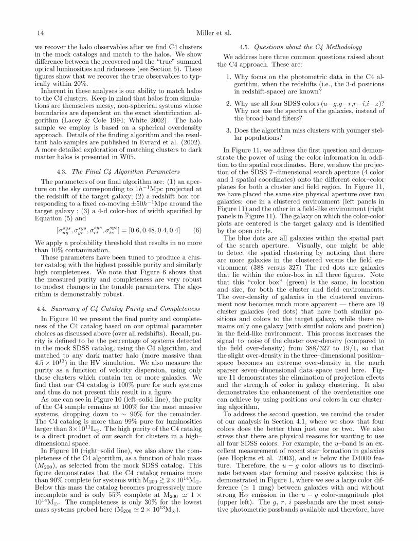
we recover the halo observables after we find C4 clustersin the mock catalogs and match to the halos. We showdifference between the recovered and the “true” summedoptical luminosities and richnesses (see Section 5). Thesefigures show that we recover the true observables to typ-ically within 20%.

Inherent in these analyses is our ability to match halosto the C4 clusters. Keep in mind that halos from simula-tions are themselves messy, non-spherical systems whoseboundaries are dependent on the exact identification al-gorithm (Lacey & Cole 1994; White 2002). The halosample we employ is based on a spherical overdensityapproach. Details of the finding algorithm and the resul-tant halo samples are published in Evrard et al. (2002).A more detailed exploration of matching clusters to darkmatter halos is presented in W05.

4.3. The Final C4 Algorithm Parameters

The parameters of our final algorithm are: (1) an aper-ture on the sky corresponding to 1h−1Mpc projected atthe redshift of the target galaxy; (2) a redshift box cor-responding to a fixed co-moving ±50h−1Mpc around thetarget galaxy ; (3) a 4-d color-box of width specified byEquation (5) and

[σsysug , σsys

gr , σsysri , σsys

iz ] = [0.6, 0.48, 0.4, 0.4] (6)

We apply a probability threshold that results in no morethan 10% contamination.

These parameters have been tuned to produce a clus-ter catalog with the highest possible purity and similarlyhigh completeness. We note that Figure 6 shows thatthe measured purity and completeness are very robustto modest changes in the tunable parameters. The algo-rithm is demonstrably robust.

4.4. Summary of C4 Catalog Purity and Completeness

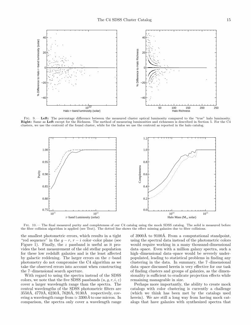
In Figure 10 we present the final purity and complete-ness of the C4 catalog based on our optimal parameterchoices as discussed above (over all redshifts). Recall, pu-rity is defined to be the percentage of systems detectedin the mock SDSS catalog, using the C4 algorithm, andmatched to any dark matter halo (more massive than4.5 × 1013) in the HV simulation. We also measure thepurity as a function of velocity dispersion, using onlythose clusters which contain ten or more galaxies. Wefind that our C4 catalog is 100% pure for such systemsand thus do not present this result in a figure.

As one can see in Figure 10 (left–solid line), the purityof the C4 sample remains at 100% for the most massivesystems, dropping down to ∼ 90% for the remainder.The C4 catalog is more than 99% pure for luminositieslarger than 3×1011L⊙. The high purity of the C4 catalogis a direct product of our search for clusters in a high–dimensional space.

In Figure 10 (right–solid line), we also show the com-pleteness of the C4 algorithm, as a function of halo mass(M200), as selected from the mock SDSS catalog. Thisfigure demonstrates that the C4 catalog remains morethan 90% complete for systems with M200 >

∼ 2×1014M⊙.Below this mass the catalog becomes progressively moreincomplete and is only 55% complete at M200 ≃ 1 ×

1014M⊙. The completeness is only 30% for the lowestmass systems probed here (M200 ≃ 2 × 1013M⊙).

4.5. Questions about the C4 Methodology

We address here three common questions raised aboutthe C4 approach. These are:

1. Why focus on the photometric data in the C4 al-gorithm, when the redshifts (i.e., the 3-d positionsin redshift-space) are known?

2. Why use all four SDSS colors (u−g,g−r,r−i,i−z)?Why not use the spectra of the galaxies, instead ofthe broad-band filters?

3. Does the algorithm miss clusters with younger stel-lar populations?

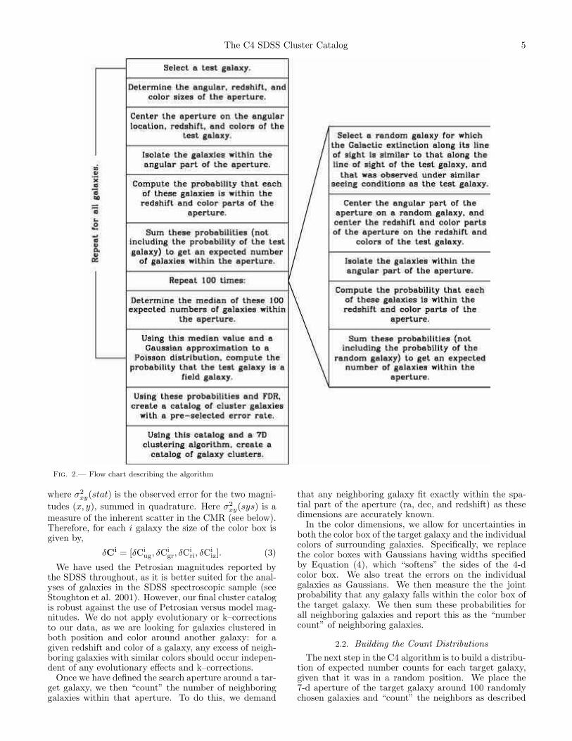
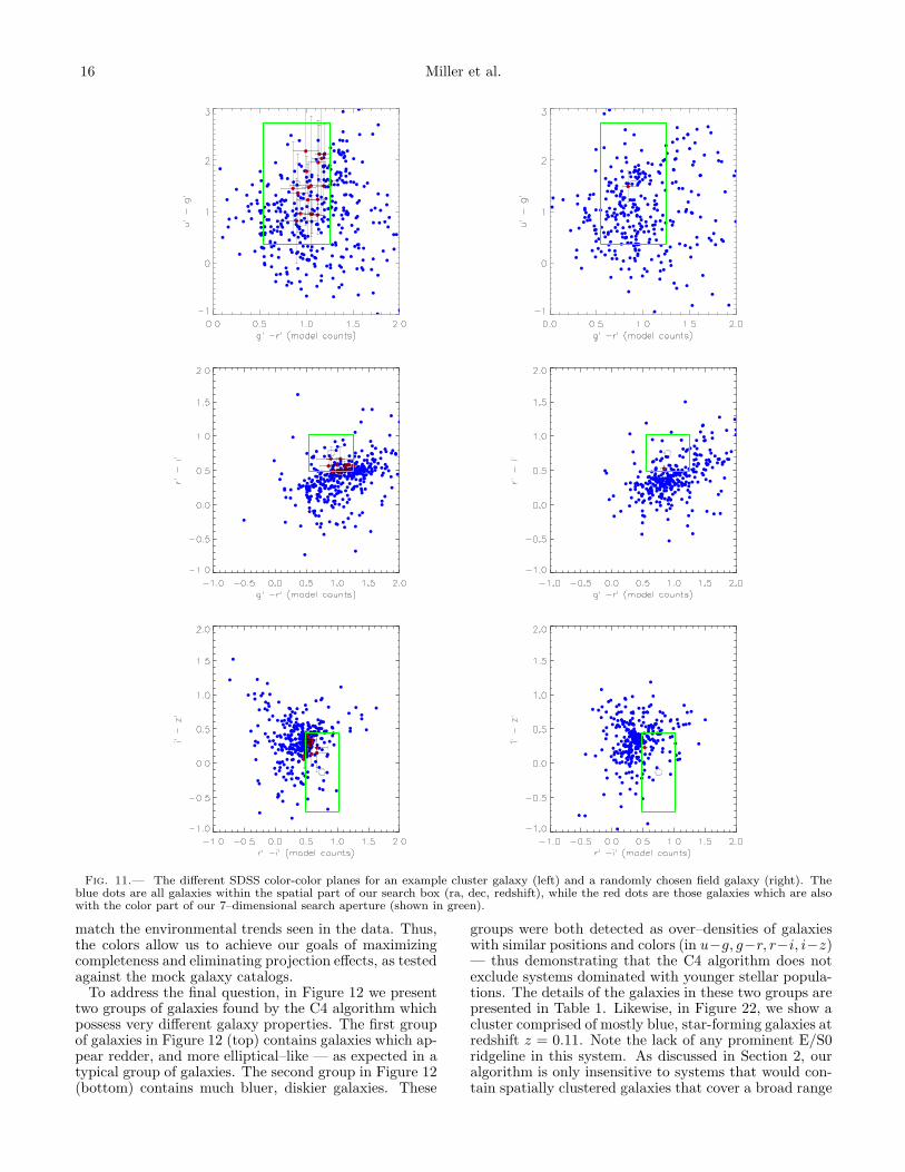
In Figure 11, we address the first question and demon-strate the power of using the color information in addi-tion to the spatial coordinates. Here, we show the projec-tion of the SDSS 7–dimensional search aperture (4 colorand 1 spatial coordinates) onto the different color–colorplanes for both a cluster and field region. In Figure 11,we have placed the same size physical aperture over twogalaxies: one in a clustered environment (left panels inFigure 11) and the other in a field-like environment (rightpanels in Figure 11). The galaxy on which the color-colorplots are centered is the target galaxy and is identifiedby the open circle.

The blue dots are all galaxies within the spatial partof the search aperture. Visually, one might be ableto detect the spatial clustering by noticing that thereare more galaxies in the clustered versus the field en-vironment (388 versus 327) The red dots are galaxiesthat lie within the color-box in all three figures. Notethat this “color box” (green) is the same, in locationand size, for both the cluster and field environments.The over-density of galaxies in the clustered environ-ment now becomes much more apparent — there are 19cluster galaxies (red dots) that have both similar po-sitions and colors to the target galaxy, while there re-mains only one galaxy (with similar colors and position)in the field-like environment. This process increases thesignal–to–noise of the cluster over-density (compared tothe field over-density) from 388/327 to 19/1, so thatthe slight over-density in the three–dimensional position–space becomes an extreme over-density in the muchsparser seven–dimensional data–space used here. Fig-ure 11 demonstrates the elimination of projection effectsand the strength of color in galaxy clustering. It alsodemonstrates the enhancement of the overdensities onecan achieve by using positions and colors in our cluster-ing algorithm,

To address the second question, we remind the readerof our analysis in Section 4.1, where we show that fourcolors does the better than just one or two. We alsostress that there are physical reasons for wanting to useall four SDSS colors. For example, the u–band is an ex-cellent measurement of recent star–formation in galaxies(see Hopkins et al. 2003), and is below the D4000 fea-ture. Therefore, the u − g color allows us to discrimi-nate between star–forming and passive galaxies; this isdemonstrated in Figure 1, where we see a large color dif-ference (≃ 1 mag) between galaxies with and withoutstrong Hα emission in the u − g color-magnitude plot(upper left). The g, r, i passbands are the most sensi-tive photometric passbands available and therefore, have

The C4 SDSS Cluster Catalog 15

1012

Halo r−band luminosity (solar)

−40

−20

0

20

40%

Diff

eren

ce to

Hal

o r−

band

lum

inos

ity (

sola

r)

50 100 150 200 250Halo Richness

−40

−20

0

20

40

% D

iffer

ence

to H

alo

Ric

hnes

s

Fig. 9.— Left: The percentage difference between the measured cluster optical luminosity compared to the “true” halo luminosity.Right: Same as Left except for the Richness. The method of measuring luminosities and richnesses is described in Section 5. For the C4clusters, we use the centroid of the found cluster, while for the halos we use the centroid as reported in the halo catalog.

1011 1012

r−band Luminosity (solar)

0.75

0.80

0.85

0.90

0.95

1.00

Pur

ity

1014 1015

Halo Mass (M200 solar)

0.0

0.2

0.4

0.6

0.8

1.0

1.2C

ompl

eten

ess

Fig. 10.— The final measured purity and completeness of our C4 catalog using the mock SDSS catalog. The solid is measured beforethe fiber collision algorithm is applied (see Text). The dotted line shows the effect missing galaxies due to fiber collisions.

the smallest photometric errors, which results in a tight“red sequence” in the g − r, r − i color–color plane (seeFigure 1). Finally, the z passband is useful as it pro-vides the best measurement of the old stellar populationfor these low redshift galaxies and is the least affectedby galactic reddening. The larger errors on the z–bandphotometry do not compromise the C4 algorithm as wetake the observed errors into account when constructingthe 7–dimensional search aperture.

With regard to using the spectra instead of the SDSScolors, we note that the five SDSS passbands (u, g, r, i, z)cover a larger wavelength range than the spectra. Thecentral wavelengths of the SDSS photometric filters are3550A, 4770A, 6230A, 7620A, 9130A respectively, cov-ering a wavelength range from ≃ 3300A to one micron. Incomparison, the spectra only cover a wavelength range

of 3900A to 9100A. From a computational standpoint,using the spectral data instead of the photometric colorswould require working in a many thousand-dimensionaldata–space. Even with a million galaxy spectra, such ahigh–dimensional data–space would be severely under-populated, leading to statistical problems in finding anyclustering in the data. In summary, the 7–dimensionaldata–space discussed herein is very effective for our taskof finding clusters and groups of galaxies, as the dimen-sionality is sufficient to eradicate projection effects whileremaining manageable in size.

Perhaps more importantly, the ability to create mockcatalogs with color clustering is currently a challenge(which we think has been met by the catalogs usedherein). We are still a long way from having mock cat-alogs that have galaxies with synthesized spectra that

16 Miller et al.

Fig. 11.— The different SDSS color-color planes for an example cluster galaxy (left) and a randomly chosen field galaxy (right). Theblue dots are all galaxies within the spatial part of our search box (ra, dec, redshift), while the red dots are those galaxies which are alsowith the color part of our 7–dimensional search aperture (shown in green).

match the environmental trends seen in the data. Thus,the colors allow us to achieve our goals of maximizingcompleteness and eliminating projection effects, as testedagainst the mock galaxy catalogs.

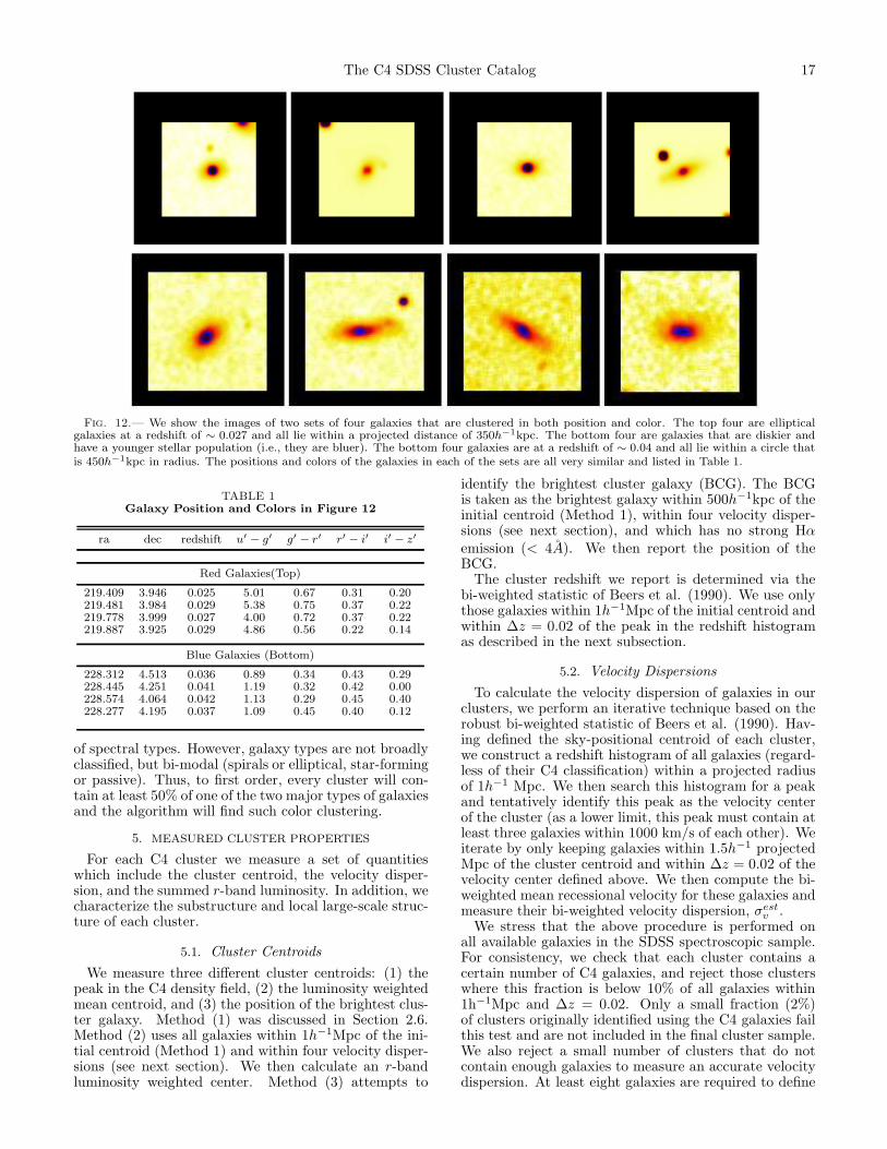
To address the final question, in Figure 12 we presenttwo groups of galaxies found by the C4 algorithm whichpossess very different galaxy properties. The first groupof galaxies in Figure 12 (top) contains galaxies which ap-pear redder, and more elliptical–like — as expected in atypical group of galaxies. The second group in Figure 12(bottom) contains much bluer, diskier galaxies. These

groups were both detected as over–densities of galaxieswith similar positions and colors (in u−g, g−r, r−i, i−z)— thus demonstrating that the C4 algorithm does notexclude systems dominated with younger stellar popula-tions. The details of the galaxies in these two groups arepresented in Table 1. Likewise, in Figure 22, we show acluster comprised of mostly blue, star-forming galaxies atredshift z = 0.11. Note the lack of any prominent E/S0ridgeline in this system. As discussed in Section 2, ouralgorithm is only insensitive to systems that would con-tain spatially clustered galaxies that cover a broad range

The C4 SDSS Cluster Catalog 17

Fig. 12.— We show the images of two sets of four galaxies that are clustered in both position and color. The top four are ellipticalgalaxies at a redshift of ∼ 0.027 and all lie within a projected distance of 350h−1kpc. The bottom four are galaxies that are diskier andhave a younger stellar population (i.e., they are bluer). The bottom four galaxies are at a redshift of ∼ 0.04 and all lie within a circle thatis 450h−1kpc in radius. The positions and colors of the galaxies in each of the sets are all very similar and listed in Table 1.

TABLE 1Galaxy Position and Colors in Figure 12

ra dec redshift u′ − g′ g′ − r′ r′ − i′ i′ − z′

Red Galaxies(Top)

219.409 3.946 0.025 5.01 0.67 0.31 0.20219.481 3.984 0.029 5.38 0.75 0.37 0.22219.778 3.999 0.027 4.00 0.72 0.37 0.22219.887 3.925 0.029 4.86 0.56 0.22 0.14

Blue Galaxies (Bottom)

228.312 4.513 0.036 0.89 0.34 0.43 0.29228.445 4.251 0.041 1.19 0.32 0.42 0.00228.574 4.064 0.042 1.13 0.29 0.45 0.40228.277 4.195 0.037 1.09 0.45 0.40 0.12

of spectral types. However, galaxy types are not broadlyclassified, but bi-modal (spirals or elliptical, star-formingor passive). Thus, to first order, every cluster will con-tain at least 50% of one of the two major types of galaxiesand the algorithm will find such color clustering.

5. MEASURED CLUSTER PROPERTIES

For each C4 cluster we measure a set of quantitieswhich include the cluster centroid, the velocity disper-sion, and the summed r-band luminosity. In addition, wecharacterize the substructure and local large-scale struc-ture of each cluster.

5.1. Cluster Centroids

We measure three different cluster centroids: (1) thepeak in the C4 density field, (2) the luminosity weightedmean centroid, and (3) the position of the brightest clus-ter galaxy. Method (1) was discussed in Section 2.6.Method (2) uses all galaxies within 1h−1Mpc of the ini-tial centroid (Method 1) and within four velocity disper-sions (see next section). We then calculate an r-bandluminosity weighted center. Method (3) attempts to

identify the brightest cluster galaxy (BCG). The BCGis taken as the brightest galaxy within 500h−1kpc of theinitial centroid (Method 1), within four velocity disper-sions (see next section), and which has no strong Hαemission (< 4A). We then report the position of theBCG.

The cluster redshift we report is determined via thebi-weighted statistic of Beers et al. (1990). We use onlythose galaxies within 1h−1Mpc of the initial centroid andwithin ∆z = 0.02 of the peak in the redshift histogramas described in the next subsection.

5.2. Velocity Dispersions

To calculate the velocity dispersion of galaxies in ourclusters, we perform an iterative technique based on therobust bi-weighted statistic of Beers et al. (1990). Hav-ing defined the sky-positional centroid of each cluster,we construct a redshift histogram of all galaxies (regard-less of their C4 classification) within a projected radiusof 1h−1 Mpc. We then search this histogram for a peakand tentatively identify this peak as the velocity centerof the cluster (as a lower limit, this peak must contain atleast three galaxies within 1000 km/s of each other). Weiterate by only keeping galaxies within 1.5h−1 projectedMpc of the cluster centroid and within ∆z = 0.02 of thevelocity center defined above. We then compute the bi-weighted mean recessional velocity for these galaxies andmeasure their bi-weighted velocity dispersion, σest

v .We stress that the above procedure is performed on

all available galaxies in the SDSS spectroscopic sample.For consistency, we check that each cluster contains acertain number of C4 galaxies, and reject those clusterswhere this fraction is below 10% of all galaxies within1h−1Mpc and ∆z = 0.02. Only a small fraction (2%)of clusters originally identified using the C4 galaxies failthis test and are not included in the final cluster sample.We also reject a small number of clusters that do notcontain enough galaxies to measure an accurate velocitydispersion. At least eight galaxies are required to define

18 Miller et al.

the velocity dispersion, consistent with previous limits toget a reliable value (see Collins et al. 1995). Note thatmost (80%) of our clusters in the real SDSS data con-tain ≥ 20 galaxies with which to measure the velocitydispersion. Clusters which do not meet this criteria areremoved from the main sample. To get our final veloc-ity dispersion measurements (σv), we re-calculate it foreach cluster using only galaxies within four times the es-timated velocity dispersion (σest

v ) discussed above. Thisis similar to the standard sigma-clipping method used inthe literature. The accuracy of these final measurements,which are in the observed reference frame, are discussedbelow.

5.3. Summed Optical Cluster Luminosity

To calculate the total summed r–band optical luminos-ity for each cluster, we convert the apparent magnitudesof all cluster members into optical luminosities, using theconversions in Fukugita et al. (1996), and sum them. Allmagnitudes are k-corrected according to Blanton et al.(2003a) and extinction corrected according to Schlegel,Finkbeiner, and Davis (1998). Cluster membership isconfined to galaxies within 4σv in redshift–space and aprojected radius of 1.5h−1Mpc on the sky. The SDSSmain galaxy sample is designed to be complete (> 95%)to mr = 17.77 and the C4 cluster sample is complete(> 90%) to z = 0.11. Thus, to minimize effects from theSDSS selection function, we use an absolute magnitudelimit of Mr < −19.9, which is an apparent magnitude ofmr = 17.8 at z ≃ 0.11, when measuring the optical lumi-nosities. Clusters beyond z = 0.11 will need to have theiroptical luminosities corrected for this incompleteness.

5.4. Structure Contamination Flag

We define a “Structure Contamination Flag” (SCF)to measure the degree of isolation in redshift–spacefor each cluster. Specifically, we examine radial varia-tions of the velocity dispersion for each cluster, notinglarge radial variations from the mean velocity disper-sion. Clusters which are embedded in surrounding large-scale structure can have significant velocity contamina-tion. SCF increases with increasing standard deviationsin the velocity dispersion profiles. We calculate the bi-weight velocity dispersion within 500,1000,1500,2000 and2500h−1kpc radial bins as described above, and deter-mine the standard deviation. We then assign an SCFbased on the ratio of the standard deviation of the dis-persions over the mean of the velocity dispersions. Weuse three bins, SCF = [0,2], in approximating the bot-tom, middle, and top thirds of the distribution of theratio. A cluster with SCF = 0 has a ratio less than 15%whereas SCF = 2 has a ratio > 30%. The sky plot andvelocity profile are shown for a real SDSS cluster with ahigh SCF=2 cluster in Figure 21, 23, and 24. Notice thatthe velocity dispersion as a function of radius is highlyerratic, producing a large standard deviation about themean. Figures 23 and 24 show two clusters separatedby less then two tenths of one degree and ∆z = 0.01.Notice that the velocity dispersion profile increases sys-tematically as the galaxies from the neighboring systemare picked up with increasing aperture. These clustersboth have SCF = 2. A clusters with SCF = 1 is shownin Figure 22 and with SCF = 0 in 25. Notice here thatthe velocity dispersion profiles are nearly constant. This

SCF flag does not necessarily quantify the substructureof the main cluster, but rather identifies clusters whosevelocity dispersions may be inaccurate because of nearbylarge-scale structure.

5.5. Dressler-Shectman Statistic

In addition to quantifying the local large–scale struc-ture for each cluster, we can use the Dressler-Shectmansubstructure statistic to search for local differences in acluster’s mean recession velocity and velocity dispersion.For each cluster member (within 1.5h−1Mpc and 4σv),we compute a local recession velocity and local velocitydispersion using the ten nearest neighbors to the galaxywhich are also within 4σv of the cluster redshift. Wethen compute the difference between these local quanti-ties and the mean recession velocity and velocity disper-sion for the whole cluster. The cumulative differences arethen used as a measure of the cluster substructure. Tocompute the significance of this measurement, we shufflethe galaxy velocities within the cluster and repeat the ex-ercise 1000 times. Using these Monte-Carlo realizations,we calculate the probability that the observed cumulativedifferences would be obtained at random, given the spa-tial positions of the galaxies. A low probability indicatesthat the substructure is significant. For more details,see Dressler and Shectman (1988) and Oegerle and Hill(2001).

6. SCALING RELATIONS AND THEIR SCATTER

Any galaxy cluster catalog will have observables thatcan be related to the underlying halo dark matter mass.Typically, researchers have used some sort of galaxy num-ber count, i.e., richness (Abell 1958, Yee and Ellingson2003). While the C4 clusters certainly have galaxy num-ber counts, we also measure the summed r-band lumi-nosity of the galaxies within each cluster. We addition-ally measure a velocity dispersion for all clusters withinour spectroscopic data (using 8 or more galaxy mem-bers within a projected radius of 1h−1Mpc and withinfour velocity dispersions). In this section, we determinewhich cluster observables scale best with the halo massesin the mock galaxy catalogs. We stress that this sec-tion does not quantify any absolute scaling-laws (or theirscatter), which requires a detailed analysis of the role ofcosmology and of the sensitivity of this scaling to thehalo occupation. This will be presented in an upcomingpaper. Here, we simply study how the scatter changesas we vary parameters of the cluster finding algorithmand measures of the local foreground/background con-tamination. In short, the scaling relations presented inthis section are used solely to guide our choice of the bestcluster observable when relating to mass, as qualified bythe scatter, and we caution the reader not to use themto draw cosmologically-dependent conclusions.

6.1. Structure Contamination and Velocity Dispersion

For virialized systems, the velocity dispersion is an ob-vious choice when attempting to measure the mass of acluster. So first, we examine the validity of our method torecover the velocity dispersions. In Figure 13, we com-pare our measured velocity dispersions for C4 clustersin the mock catalog against the known particle line-of-sight velocity dispersions for the halos in the simulations.We use only clusters with 10 or more galaxies within

The C4 SDSS Cluster Catalog 19

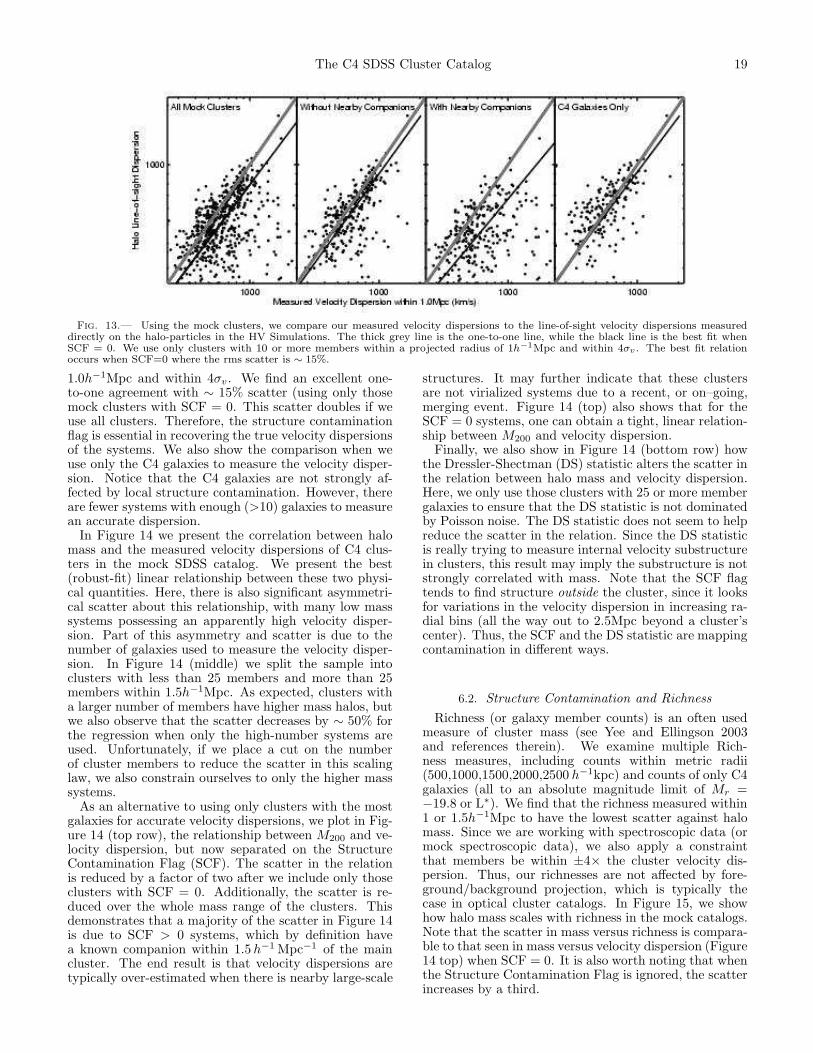
Fig. 13.— Using the mock clusters, we compare our measured velocity dispersions to the line-of-sight velocity dispersions measureddirectly on the halo-particles in the HV Simulations. The thick grey line is the one-to-one line, while the black line is the best fit whenSCF = 0. We use only clusters with 10 or more members within a projected radius of 1h−1Mpc and within 4σv . The best fit relationoccurs when SCF=0 where the rms scatter is ∼ 15%.

1.0h−1Mpc and within 4σv. We find an excellent one-to-one agreement with ∼ 15% scatter (using only thosemock clusters with SCF = 0. This scatter doubles if weuse all clusters. Therefore, the structure contaminationflag is essential in recovering the true velocity dispersionsof the systems. We also show the comparison when weuse only the C4 galaxies to measure the velocity disper-sion. Notice that the C4 galaxies are not strongly af-fected by local structure contamination. However, thereare fewer systems with enough (>10) galaxies to measurean accurate dispersion.

In Figure 14 we present the correlation between halomass and the measured velocity dispersions of C4 clus-ters in the mock SDSS catalog. We present the best(robust-fit) linear relationship between these two physi-cal quantities. Here, there is also significant asymmetri-cal scatter about this relationship, with many low masssystems possessing an apparently high velocity disper-sion. Part of this asymmetry and scatter is due to thenumber of galaxies used to measure the velocity disper-sion. In Figure 14 (middle) we split the sample intoclusters with less than 25 members and more than 25members within 1.5h−1Mpc. As expected, clusters witha larger number of members have higher mass halos, butwe also observe that the scatter decreases by ∼ 50% forthe regression when only the high-number systems areused. Unfortunately, if we place a cut on the numberof cluster members to reduce the scatter in this scalinglaw, we also constrain ourselves to only the higher masssystems.

As an alternative to using only clusters with the mostgalaxies for accurate velocity dispersions, we plot in Fig-ure 14 (top row), the relationship between M200 and ve-locity dispersion, but now separated on the StructureContamination Flag (SCF). The scatter in the relationis reduced by a factor of two after we include only thoseclusters with SCF = 0. Additionally, the scatter is re-duced over the whole mass range of the clusters. Thisdemonstrates that a majority of the scatter in Figure 14is due to SCF > 0 systems, which by definition havea known companion within 1.5 h−1 Mpc−1 of the maincluster. The end result is that velocity dispersions aretypically over-estimated when there is nearby large-scale

structures. It may further indicate that these clustersare not virialized systems due to a recent, or on–going,merging event. Figure 14 (top) also shows that for theSCF = 0 systems, one can obtain a tight, linear relation-ship between M200 and velocity dispersion.

Finally, we also show in Figure 14 (bottom row) howthe Dressler-Shectman (DS) statistic alters the scatter inthe relation between halo mass and velocity dispersion.Here, we only use those clusters with 25 or more membergalaxies to ensure that the DS statistic is not dominatedby Poisson noise. The DS statistic does not seem to helpreduce the scatter in the relation. Since the DS statisticis really trying to measure internal velocity substructurein clusters, this result may imply the substructure is notstrongly correlated with mass. Note that the SCF flagtends to find structure outside the cluster, since it looksfor variations in the velocity dispersion in increasing ra-dial bins (all the way out to 2.5Mpc beyond a cluster’scenter). Thus, the SCF and the DS statistic are mappingcontamination in different ways.

6.2. Structure Contamination and Richness

Richness (or galaxy member counts) is an often usedmeasure of cluster mass (see Yee and Ellingson 2003and references therein). We examine multiple Rich-ness measures, including counts within metric radii(500,1000,1500,2000,2500 h−1kpc) and counts of only C4galaxies (all to an absolute magnitude limit of Mr =−19.8 or L∗). We find that the richness measured within1 or 1.5h−1Mpc to have the lowest scatter against halomass. Since we are working with spectroscopic data (ormock spectroscopic data), we also apply a constraintthat members be within ±4× the cluster velocity dis-persion. Thus, our richnesses are not affected by fore-ground/background projection, which is typically thecase in optical cluster catalogs. In Figure 15, we showhow halo mass scales with richness in the mock catalogs.Note that the scatter in mass versus richness is compara-ble to that seen in mass versus velocity dispersion (Figure14 top) when SCF = 0. It is also worth noting that whenthe Structure Contamination Flag is ignored, the scatterincreases by a third.

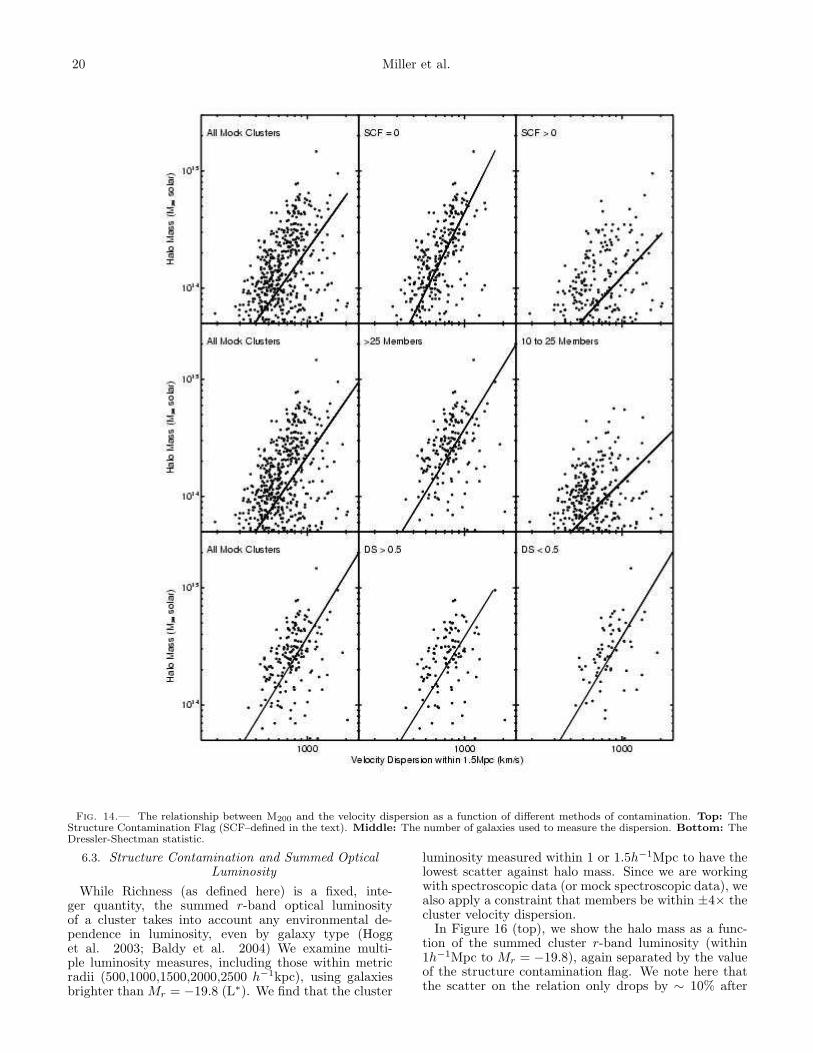
20 Miller et al.

Fig. 14.— The relationship between M200 and the velocity dispersion as a function of different methods of contamination. Top: TheStructure Contamination Flag (SCF–defined in the text). Middle: The number of galaxies used to measure the dispersion. Bottom: TheDressler-Shectman statistic.

6.3. Structure Contamination and Summed OpticalLuminosity

While Richness (as defined here) is a fixed, inte-ger quantity, the summed r-band optical luminosityof a cluster takes into account any environmental de-pendence in luminosity, even by galaxy type (Hogget al. 2003; Baldy et al. 2004) We examine multi-ple luminosity measures, including those within metricradii (500,1000,1500,2000,2500 h−1kpc), using galaxiesbrighter than Mr = −19.8 (L∗). We find that the cluster

luminosity measured within 1 or 1.5h−1Mpc to have thelowest scatter against halo mass. Since we are workingwith spectroscopic data (or mock spectroscopic data), wealso apply a constraint that members be within ±4× thecluster velocity dispersion.

In Figure 16 (top), we show the halo mass as a func-tion of the summed cluster r-band luminosity (within1h−1Mpc to Mr = −19.8), again separated by the valueof the structure contamination flag. We note here thatthe scatter on the relation only drops by ∼ 10% after

The C4 SDSS Cluster Catalog 21

Fig. 15.— Using the mock clusters, we plot the relationship between the richness as measured with 1h−1Mpc and for members within±4 velocity dispersions of the cluster, against halo mass (top) or velocity dispersion (bottom). We show the effect of the StructureContamination Flag (SCF). The best-fit relation is for all clusters without a nearby companion.

applying the SCF cut, demonstrating that the summedluminosity as a proxy to cluster mass is less contaminatedby nearby large-scale structure than velocity dispersion.We also note that the scatter is smaller for mass-versus-luminosity than it is for either mass-richness or mass-velocity dispersion. Thus, we conclude that in the mockcatalogs, the summed r-band luminosity is the best mea-sure of the cluster dark matter halo mass.

Figure 17 shows the halo mass as a function of thesummed r-band cluster luminosity with a variety of best-fit relations and their scatter. We observe a linear corre-lation between mass and optical cluster luminosity andthe best robust-fit linear relationships (mass versus lu-minosity and luminosity versus mass) are shown (light-gray solid and dashed line respectively). One mightnotice that the relation is not precisely linear, and sowe have also used a nonparametric technique to moreaccurately trace this scaling relation (solid black-line).We plot a one-sigma confidence band around our bestnon-parametric fit (black dashed-line). The simultane-ous bands were determined using the method of Sun andLoader (1994). The gray-shaded band is the one-sigmascatter in this relation and includes effects from match-

ing (Section 4.2), measurement error, and any intrinsicscatter in the relationship.

As a consistency check, we present in Figures 16 andFigures 15 (bottom) the correlation between the velocitydispersion and richness or summed total cluster r−bandluminosity for clusters in our mock SDSS dataset. Asseen in Figure 14, the scatter is similarly reduced by afactor of two when we use only SCF=0 clusters. Ourconclusion is the same as above: our velocity dispersionscan be over-estimated when there is intervening large-scale structure to interfere with the measurement of thevelocity dispersion.

In the above sections (5 and 6), we have examinedhow foreground/background contamination from large-scale structure (or other clusters) affects the observablesof velocity dispersion, richness, and optical luminosity.We pointed out a few example clusters where the struc-ture contamination flag (SCF) varies from 0 to 2, thusdestroying any clean measure of the velocity dispersion.We showed the scaling laws which use the summed r-band luminosity and/or richness are less affected by lo-cal large-scale structure than velocity dispersion. Weconclude that the optical luminosity is the cleanest ob-

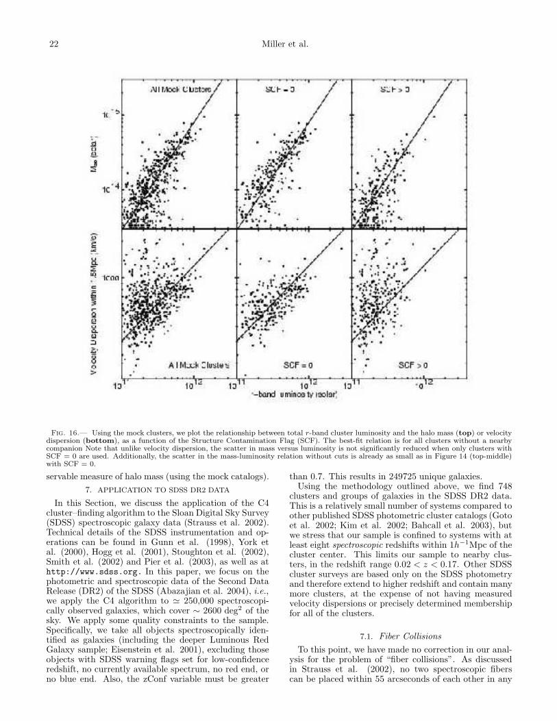
22 Miller et al.

Fig. 16.— Using the mock clusters, we plot the relationship between total r-band cluster luminosity and the halo mass (top) or velocitydispersion (bottom), as a function of the Structure Contamination Flag (SCF). The best-fit relation is for all clusters without a nearbycompanion Note that unlike velocity dispersion, the scatter in mass versus luminosity is not significantly reduced when only clusters withSCF = 0 are used. Additionally, the scatter in the mass-luminosity relation without cuts is already as small as in Figure 14 (top-middle)with SCF = 0.

servable measure of halo mass (using the mock catalogs).

7. APPLICATION TO SDSS DR2 DATA

In this Section, we discuss the application of the C4cluster–finding algorithm to the Sloan Digital Sky Survey(SDSS) spectroscopic galaxy data (Strauss et al. 2002).Technical details of the SDSS instrumentation and op-erations can be found in Gunn et al. (1998), York etal. (2000), Hogg et al. (2001), Stoughton et al. (2002),Smith et al. (2002) and Pier et al. (2003), as well as athttp://www.sdss.org. In this paper, we focus on thephotometric and spectroscopic data of the Second DataRelease (DR2) of the SDSS (Abazajian et al. 2004), i.e.,we apply the C4 algorithm to ≃ 250,000 spectroscopi-cally observed galaxies, which cover ∼ 2600 deg2 of thesky. We apply some quality constraints to the sample.Specifically, we take all objects spectroscopically iden-tified as galaxies (including the deeper Luminous RedGalaxy sample; Eisenstein et al. 2001), excluding thoseobjects with SDSS warning flags set for low-confidenceredshift, no currently available spectrum, no red end, orno blue end. Also, the zConf variable must be greater

than 0.7. This results in 249725 unique galaxies.Using the methodology outlined above, we find 748

clusters and groups of galaxies in the SDSS DR2 data.This is a relatively small number of systems compared toother published SDSS photometric cluster catalogs (Gotoet al. 2002; Kim et al. 2002; Bahcall et al. 2003), butwe stress that our sample is confined to systems with atleast eight spectroscopic redshifts within 1h−1Mpc of thecluster center. This limits our sample to nearby clus-ters, in the redshift range 0.02 < z < 0.17. Other SDSScluster surveys are based only on the SDSS photometryand therefore extend to higher redshift and contain manymore clusters, at the expense of not having measuredvelocity dispersions or precisely determined membershipfor all of the clusters.

7.1. Fiber Collisions

To this point, we have made no correction in our anal-ysis for the problem of “fiber collisions”. As discussedin Strauss et al. (2002), no two spectroscopic fiberscan be placed within 55 arcseconds of each other in any

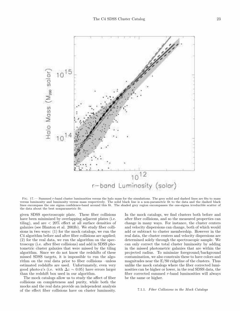
The C4 SDSS Cluster Catalog 23

Fig. 17.— Summed r-band cluster luminosities versus the halo mass for the simulations. The grey solid and dashed lines are fits to massversus luminosity and luminosity versus mass respectively. The solid black line is a non-parametric fit to the data and the dashed blacklines encompass the one sigma confidence-band around this fit. The shaded grey region encompasses the one-sigma irreducible scatter ofthe data about the best nonparametric fit.

given SDSS spectroscopic plate. These fiber collisionshave been minimized by overlapping adjacent plates (i.e.tiling), and are < 20% effect at all surface densities ofgalaxies (see Blanton et al. 2003b). We study fiber colli-sions in two ways: (1) for the mock catalogs, we run theC4 algorithm before and after fiber collisions are applied;(2) for the real data, we run the algorithm on the spec-troscopy (i.e. after fiber collisions) and add in SDSS pho-tometric cluster galaxies that were missed by the tilingalgorithm. Since we do not know the redshifts of thesemissed SDSS targets, it is impossible to run the algo-rithm on the real data prior to fiber collisions –unlessestimated redshifts are used. Unfortunately, even verygood photo-z’s (i.e. with ∆z ∼ 0.05) have errors largerthan the redshift box used in our algorithm.

The mock catalogs allow us to study the affect of fibercollisions on completeness and purity, while both themocks and the real data provide an independent analysisof the effect fiber collisions have on cluster luminosity.

In the mock catalogs, we find clusters both before andafter fiber collisions, and so the measured properties canchange in many ways. For instance, the cluster centersand velocity dispersions can change, both of which wouldadd or subtract to cluster membership. However in thereal data, the cluster centers and velocity dispersions aredetermined solely through the spectroscopic sample. Wecan only correct the total cluster luminosity by addingin the missed photometric galaxies that are within theprojected radius. To minimize foreground/backgroundcontamination, we also constrain these to have colors andmagnitudes near the E/S0 ridgeline of the clusters. Thusunlike the mock catalogs where the fiber corrected lumi-nosities can be higher or lower, in the real SDSS data, thefiber corrected summed r-band luminosities will alwaysbe the same or higher.

7.1.1. Fiber Collisions in the Mock Catalogs

24 Miller et al.

To create our mock catalogs with fiber collisions, wefind all mock galaxy pairs within 55 arcseconds and ran-domly choose the brightest galaxy in each pair. We dothis such that 70% of all galaxies with nearest-neighborseparations of less than 55 arcseconds are retained. Thismimics (albeit conservatively) the targeting algorithmdescribed in Blanton et al. (2003b). We then re-ranour cluster finder on these revised mock catalogs.

We find that regardless of fiber collisions, the complete-ness and purity remain unchanged for the more massivesystems. As the mass (or luminosity) of the clusters de-creases, the completeness after applying fiber collisionsdrops slightly (∼ 5%). As a consequence of finding fewersystems, the purity increases slightly after fiber collisionsare applied (again by 5%). This can be seen in Figure10 where the solid (dashed) lines are before (after) fibercollisions. Thus, fiber collisions play a very minimal rolein finding clusters.

However, the summed optical r-band luminosities aresystematically underestimated as seen in Figure 18 Top.In this figure we show the difference in the measuredmock cluster luminosities before and after (i.e. minus)the fiber collision algorithm is applied. Bright massiveclusters are more affected then small dim clusters. Thehistogram has been normalized to the average number ofclusters with differences between zero and ten percent.As indicated by the peak of the histogram, many of thecluster luminosities remain unchanged. Most are system-atically brighter before we remove mock galaxies due tofiber collisions (as expected). A few are dimmer beforegalaxies are removed from fiber collisions. As describedabove, the clusters found after the fiber collision algo-rithm is applied have different membership criteria thanthose before (due to a different centroid or velocity dis-persion). Thus we expect a few clusters to be brighterafter galaxies are removed from the mocks.

The distribution of the histogram in Figure 18 is nota simple Gaussian. We have investigated this and findthat the sum of two Gaussians is statistically a good fit.The two Gaussians are explained by two different pop-ulations of missed targets: typical cluster galaxies andbrightest cluster galaxies (BCG). In the mock catalogs,we find that the BCG would be missed by fiber colli-sions ∼ 38% of the time. These BCGs are significantlybrighter than typical cluster galaxies and they accountfor the tail in the histogram of Figure 18. To confirmthis, we have fit the histograms of the BCGs and non-BCGs in Figure 18 separately (as shown by the dotted(BCG) and dashed (non-BCG) curves. The sum of thesetwo Gaussians (the solid line) is then a good fit to theoverall distribution. The centers of these Gaussians tellus (on average) how much fiber collisions lower the clus-ter luminosities. When the BCG is missed, clusters aredimmer by 24%, while when the BCG is spectroscopi-cally observed, clusters are dimmer by only 6%.

7.1.2. Fiber Collisions in the SDSS Data

Since we cannot find clusters in the real SDSS spec-troscopic data before fiber collisions, we attempt to cor-rect the SDSS C4 clusters by adding galaxies that weretargeted for observation, but missed due to the tilingalgorithm. We extract all galaxies within a projected1h−1Mpc of the cluster center and brighter than mr =19.6 and Mr = −19.8, where we assume the galaxies to

be at the redshift of the cluster. We then add this addi-tional galaxy light to the cluster luminosities and look fora new BCG. To avoid adding too much noise from fore-ground/background galaxies, we require these additionalgalaxies to have colors that lie within the cluster’s E/S0ridgeline and also be no more than two magnitudes dim-mer than the orginally identified brightest cluster galaxy(BCG).

In Figure 18 bottom, we show the differences in thecluster luminosities before and after the fiber corrections.Recall that by design, the corrected cluster luminosi-ties will always be as bright or brighter than before thecorrection (since we only add in galaxies from the pho-tometry). As in the mock catalogs described above, theBCGs are missed ∼ 39% of the time. Also similar to themock catalogs, the peak of the histogram is at zero differ-ence. For comparison, we over plot the Gaussians fromthe mock catalog histograms (Figure 18 top). The closematch betweem the mock catalogs and the real SDSSdata in terms of the tails of these distributions as wellas in the fraction of missed BCGs indicate that, (a) thefiber collision algorithm we use on the mock catalogs isclose to the tiling of the SDSS, and (b) that the clusterluminosity differences have two components (BCG andnon-BCG) and can be corrected.

7.2. Galaxy Deblending and Targeting

To be targeted for spectroscopy by the SDSS (Blantonet al. 2003b), a galaxy must first be identified in the pho-tometric data. Since we’re only looking at the brightestgalaxies in the SDSS, we assume that star-galaxy separa-tion is a non-issue (see Scranton et al. 2003). However forvarious reasons, the photometric deblender occasionallyfails to correctly identify a galaxy. An extreme exampleis for Abell 1539 (ra, dec = 186.5813, 62.5563), where themultiple identification of a satellite trail caused the de-blender to reach its maximum number of objects within agiven field. Thus, many galaxies within the cluster werenot identified.

While a paper presenting the SDSS deblender algo-rithm and tests is currently under preparation (Lupton etal. 2005), we made a minimal effort to quantify any SDSSdeblender issues, specifically with regards to galaxy clus-ters. To do so, we identified 110 Abell clusters within thesky coverage of the SDSS DR2 spectroscopic survey andvisually examined each one using the SDSS Sky ServerCutout tool. This web-based tool allows the user to lookat any SDSS photometric field and overlay photometricor spectroscopic SDSS galaxies (those both targeted andobserved). One can also click on the galaxies to deter-mine their redshifts, magnitudes, etc.

The purpose of this exercise was to determine whetherSDSS deblending or targeting problems could affect theC4 algorithm. To perform this analysis, we took thefollowing steps:

1. Using the SDSS Finding Chart cutout tool, look ata 7 × 7 arcminute field around each Abell clustercenter.

2. Identify the BCG, its coordinates and r-band mag-nitude.

3. Determine the fraction of spectroscopic targetsthat actually have spectroscopy.

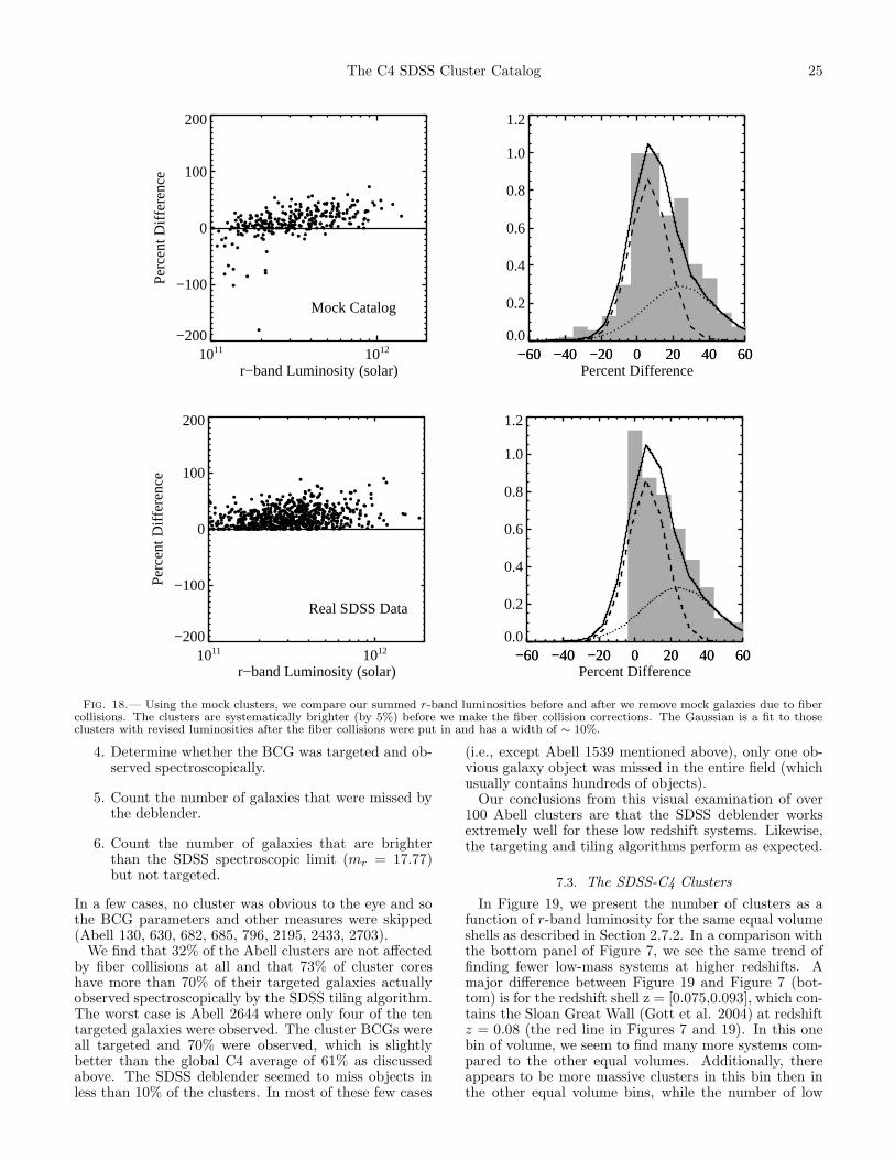
The C4 SDSS Cluster Catalog 25

1011 1012

r−band Luminosity (solar)

−200

−100

0

100

200

Per

cent

Diff

eren

ce

Mock Catalog

−60 −40 −20 0 20 40 60Percent Difference

0.0

0.2

0.4

0.6

0.8

1.0

1.2

−60 −40 −20 0 20 40 60

1011 1012

r−band Luminosity (solar)

−200

−100

0

100

200

Per

cent

Diff

eren

ce

Real SDSS Data

−60 −40 −20 0 20 40 60Percent Difference

0.0

0.2

0.4

0.6

0.8

1.0

1.2

−60 −40 −20 0 20 40 60

Fig. 18.— Using the mock clusters, we compare our summed r-band luminosities before and after we remove mock galaxies due to fibercollisions. The clusters are systematically brighter (by 5%) before we make the fiber collision corrections. The Gaussian is a fit to thoseclusters with revised luminosities after the fiber collisions were put in and has a width of ∼ 10%.

4. Determine whether the BCG was targeted and ob-served spectroscopically.

5. Count the number of galaxies that were missed bythe deblender.

6. Count the number of galaxies that are brighterthan the SDSS spectroscopic limit (mr = 17.77)but not targeted.

In a few cases, no cluster was obvious to the eye and sothe BCG parameters and other measures were skipped(Abell 130, 630, 682, 685, 796, 2195, 2433, 2703).

We find that 32% of the Abell clusters are not affectedby fiber collisions at all and that 73% of cluster coreshave more than 70% of their targeted galaxies actuallyobserved spectroscopically by the SDSS tiling algorithm.The worst case is Abell 2644 where only four of the tentargeted galaxies were observed. The cluster BCGs wereall targeted and 70% were observed, which is slightlybetter than the global C4 average of 61% as discussedabove. The SDSS deblender seemed to miss objects inless than 10% of the clusters. In most of these few cases

(i.e., except Abell 1539 mentioned above), only one ob-vious galaxy object was missed in the entire field (whichusually contains hundreds of objects).

Our conclusions from this visual examination of over100 Abell clusters are that the SDSS deblender worksextremely well for these low redshift systems. Likewise,the targeting and tiling algorithms perform as expected.

7.3. The SDSS-C4 Clusters

In Figure 19, we present the number of clusters as afunction of r-band luminosity for the same equal volumeshells as described in Section 2.7.2. In a comparison withthe bottom panel of Figure 7, we see the same trend offinding fewer low-mass systems at higher redshifts. Amajor difference between Figure 19 and Figure 7 (bot-tom) is for the redshift shell z = [0.075,0.093], which con-tains the Sloan Great Wall (Gott et al. 2004) at redshiftz = 0.08 (the red line in Figures 7 and 19). In this onebin of volume, we seem to find many more systems com-pared to the other equal volumes. Additionally, thereappears to be more massive clusters in this bin then inthe other equal volume bins, while the number of low

26 Miller et al.

1011 1012

r−band Luminosity (solar)

1

10

100N

(>

L)

Fig. 19.— The number of SDSS C4 clusters brighter than Lr

for equal volume shells, each at increasing redshift. The shells aredescribed in the text. They go from the lowest to highest redshiftas black,red, green, blue, violet. The red line covers a volumewhich includes the SDSS Great Wall (Gott et al. 2004) where wefind additional massive clusters compared to the other four equalvolumes.

mass systems is little changed.In Table 4, we present the 748 clusters detected us-

ing the C4 algorithm on the DR2 dataset. For eachcluster, we present an SDSS C4 ID (Column 1); the(J2000) right ascension and declination of the centroidvia Method (1) in Section 5.1 (Columns 2,3); the ra anddec via Method (2) in Section 5.1 (Columns 4,5); theright ascension and declination of the Brightest ClusterGalaxy (Columns 6,7);. the mean redshift of the cluster(Column 8); the velocity dispersion (to convert to therest-frame of the cluster, divide by 1 + z); (Column 9);the Richness (Column 10); the summed r-band clusterluminosity (corrected for missed targets) (Column 11);the Structure Contamination Flag (SCF; Column 12);the Dressler-Shectman substructure probability (Column13); and the names of other clusters matched to within10 arcminute of the cluster centroid (Column 14). Thenames are as follows– Abell: Abell (1958); RBS: RosatBright Source Catalog (Voges et al. 1999); RX: TheHamburg/RASS catalog of optical identifications (Badeet al. 1998); ZwCl: Zwicky compact groups and clus-ters (Zwicky and others 1961,1963,1965,1966,1968a,b);WXD: Wei et al. (1999); RXC: Oppenheimer et al.(1997); WBL: Catalog of Nearby Poor Clusters White etal. 1999); CAN: Wegman et al. (1996); SCC: Sochting etal. (2002); MACS/VMF: Vikhlinin et al.(1998); KDCS:Deep Range Survey (Postman et al. 2002). Note thatthe match is not performed against redshift, thus someof these matches are in projection only. More informa-tion on these names and additional matches can be foundon the C4 webpage.

In Figures 21 through 26, we show the sky plots, color–magnitude relations, velocity histograms, and velocitydispersion profiles for six C4 clusters detected in theDR2. We have made available these plots for all 748C4 DR2 clusters via the world-wide web. These plotsprovide for quality assurance, so users of this catalog caninspect the individual systems and determine whetherthey suit their scientific requirements.

An electronic version of the cataloggiven in Table 4 can be downloaded fromhttp://www.ctio.noao.edu/~chrism/C4/ We in-

tend to update this C4 catalog as more SDSS databecomes available and therefore, we encourage thereader to check this webpage periodically.

7.4. Comparison to Other Cluster Catalogs

In this subsection we take a closer look at the C4 clus-ter sample by comparing it to two different samples fromthe literature: the Abell (1958) catalog and the RASS-SDSS catalog (Popesso et al. 2004). These two have re-markable different selection algorithms (which are fullydescribed in their respective references). In short, theAbell catalog was created by the eyeball examinationof the optical Palomar All Sky Survey plates. On theother hand, the RASS-SDSS sample identifies the opti-cal counterparts to X-ray discovered clusters taken fromthe literature. Only 36% of the RASS-SDSS clusters arealso Abell clusters.

As opposed to the C4 catalog, neither the Abell northe RASS-SDSS cluster catalogs have selection functionsand so we can make no quantitative claims about theircompleteness or purity. However, since the C4 catalogis > 90% pure regardless of redshift and/or mass and> 90% complete for masses above 2×1014 solar massesand redshifts below z = 0.12 (see Figure 7), we expect tobe able to recover the more massive clusters from othersamples.

7.4.1. The C4-Abell Clusters

We identified those Abell clusters that lie in the area ofsky coverage for the SDSS DR2. We then match the twocluster samples and find any C4 clusters that are within10 arcminutes of an Abell cluster. We find 346 Abellclusters that meet these criteria and 123 are uniquelymatched to C4 clusters (only 5 Abell clusters are matchedto two different C4 clusters). However, to more fairlycompare the two samples, we must place a redshift con-straint on the two samples so that some minimum levelof completeness is met by the algorithms. The Abellcluster catalog is thought to be fairly complete within0.03 ≤ z ≤ 0.12 (see Miller et al. 2002). And as shownin Figure 7, the C4 sample is also > 90% complete inthis redshift range for masses greater than 2× 1014 solarmasses. When we apply this redshift constraint, thereare 104 Abell clusters and 71% of them are also found bythe C4 algorithm. We took a closer examination of the30 missing Abell clusters (see Table 2) and found thatsix of them are actually too deep for the C4 algorithm,eight have too few spectra, and six are not clusters at all(as determined through a visual examination of the pho-tometry and spectra around their Abell centers). So ifwe exclude these 20 from the list of Abell clusters the C4algorithm should be able to find, than the recovery rategoes up to 88%. If you include another three Abell clus-ters that were found, but blended into nearby clusters,the recovery rate is 92%. Thus, the the C4 algorithmcan recover ∼ 90% of Abell clusters and the ones thatare missed are typically found at redshifts where the C4algorithm is less than 90% complete (z > 0.12).

7.4.2. The RASS-SDSS-C4 Clusters

We applied the same area constraints to the Popesso etal. (2004) sample as we did to the Abell clusters. Of the97 RASS-SDSS clusters that lie within the area of the

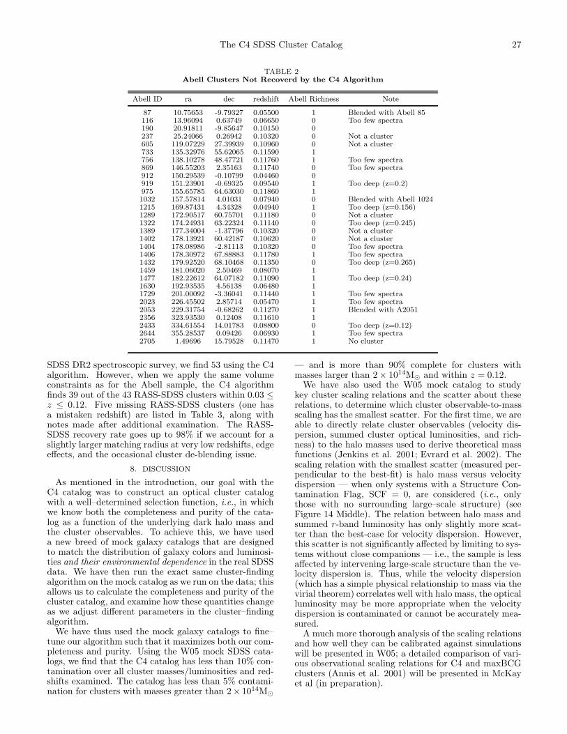
The C4 SDSS Cluster Catalog 27

TABLE 2Abell Clusters Not Recoverd by the C4 Algorithm

Abell ID ra dec redshift Abell Richness Note

87 10.75653 -9.79327 0.05500 1 Blended with Abell 85116 13.96094 0.63749 0.06650 0 Too few spectra190 20.91811 -9.85647 0.10150 0237 25.24066 0.26942 0.10320 0 Not a cluster605 119.07229 27.39939 0.10960 0 Not a cluster733 135.32976 55.62065 0.11590 1756 138.10278 48.47721 0.11760 1 Too few spectra869 146.55203 2.35163 0.11740 0 Too few spectra912 150.29539 -0.10799 0.04460 0919 151.23901 -0.69325 0.09540 1 Too deep (z=0.2)975 155.65785 64.63030 0.11860 11032 157.57814 4.01031 0.07940 0 Blended with Abell 10241215 169.87431 4.34328 0.04940 1 Too deep (z=0.156)1289 172.90517 60.75701 0.11180 0 Not a cluster1322 174.24931 63.22324 0.11140 0 Too deep (z=0.245)1389 177.34004 -1.37796 0.10320 0 Not a cluster1402 178.13921 60.42187 0.10620 0 Not a cluster1404 178.08986 -2.81113 0.10320 0 Too few spectra1406 178.30972 67.88883 0.11780 1 Too few spectra1432 179.92520 68.10468 0.11350 0 Too deep (z=0.265)1459 181.06020 2.50469 0.08070 11477 182.22612 64.07182 0.11090 1 Too deep (z=0.24)1630 192.93535 4.56138 0.06480 11729 201.00092 -3.36041 0.11440 1 Too few spectra2023 226.45502 2.85714 0.05470 1 Too few spectra2053 229.31754 -0.68262 0.11270 1 Blended with A20512356 323.93530 0.12408 0.11610 12433 334.61554 14.01783 0.08800 0 Too deep (z=0.12)2644 355.28537 0.09426 0.06930 1 Too few spectra2705 1.49696 15.79528 0.11470 1 No cluster

SDSS DR2 spectroscopic survey, we find 53 using the C4algorithm. However, when we apply the same volumeconstraints as for the Abell sample, the C4 algorithmfinds 39 out of the 43 RASS-SDSS clusters within 0.03 ≤

z ≤ 0.12. Five missing RASS-SDSS clusters (one hasa mistaken redshift) are listed in Table 3, along withnotes made after additional examination. The RASS-SDSS recovery rate goes up to 98% if we account for aslightly larger matching radius at very low redshifts, edgeeffects, and the occasional cluster de-blending issue.

8. DISCUSSION

As mentioned in the introduction, our goal with theC4 catalog was to construct an optical cluster catalogwith a well–determined selection function, i.e., in whichwe know both the completeness and purity of the cata-log as a function of the underlying dark halo mass andthe cluster observables. To achieve this, we have useda new breed of mock galaxy catalogs that are designedto match the distribution of galaxy colors and luminosi-ties and their environmental dependence in the real SDSSdata. We have then run the exact same cluster-findingalgorithm on the mock catalog as we run on the data; thisallows us to calculate the completeness and purity of thecluster catalog, and examine how these quantities changeas we adjust different parameters in the cluster–findingalgorithm.

We have thus used the mock galaxy catalogs to fine–tune our algorithm such that it maximizes both our com-pleteness and purity. Using the W05 mock SDSS cata-logs, we find that the C4 catalog has less than 10% con-tamination over all cluster masses/luminosities and red-shifts examined. The catalog has less than 5% contami-nation for clusters with masses greater than 2× 1014M⊙

— and is more than 90% complete for clusters withmasses larger than 2 × 1014M⊙ and within z = 0.12.

We have also used the W05 mock catalog to studykey cluster scaling relations and the scatter about theserelations, to determine which cluster observable-to-massscaling has the smallest scatter. For the first time, we areable to directly relate cluster observables (velocity dis-persion, summed cluster optical luminosities, and rich-ness) to the halo masses used to derive theoretical massfunctions (Jenkins et al. 2001; Evrard et al. 2002). Thescaling relation with the smallest scatter (measured per-pendicular to the best-fit) is halo mass versus velocitydispersion — when only systems with a Structure Con-tamination Flag, SCF = 0, are considered (i.e., onlythose with no surrounding large–scale structure) (seeFigure 14 Middle). The relation between halo mass andsummed r-band luminosity has only slightly more scat-ter than the best-case for velocity dispersion. However,this scatter is not significantly affected by limiting to sys-tems without close companions — i.e., the sample is lessaffected by intervening large-scale structure than the ve-locity dispersion is. Thus, while the velocity dispersion(which has a simple physical relationship to mass via thevirial theorem) correlates well with halo mass, the opticalluminosity may be more appropriate when the velocitydispersion is contaminated or cannot be accurately mea-sured.

A much more thorough analysis of the scaling relationsand how well they can be calibrated against simulationswill be presented in W05; a detailed comparison of vari-ous observational scaling relations for C4 and maxBCGclusters (Annis et al. 2001) will be presented in McKayet al (in preparation).

28 Miller et al.

TABLE 3RASS-SDSS Clusters Not Recoverd by the C4 Algorithm

RASS-SDSS ID ra dec redshift X-ray Luminosity Note

RXCJ0736.4+3925 114.10400 39.43290 0.11700 4.81×1037WRXCJ0953.6+0142 148.42310 1.71180 0.09800 0.97×1037W Blended with SDSSDR2-C4-1304RXCJ1303.9+6731 195.98540 67.51770 0.10600 0.35×1037W Too deep (z=0.22)RXCJ1511.5+0145 227.88969 1.76420 0.03700 0.07×1037W Too close to survey edgeRXCJ2324.3+1439 351.08771 14.66450 0.04200 0.97×1037W SDSSDR2-C4-2001 is 14 arcminutes away.

We present this C4 catalog to demonstrate the powerof the SDSS spectroscopic data in finding nearby clus-ters of galaxies, and to advance our understanding ofcluster scaling relations and galaxy evolution in denseenvironments (for which the sample has been used in thestudies of Gomez et al. 2003; Miller et al. 2003; Baloghet al. 2004). In future work, we will use the C4 catalogto constrain cosmological parameters and to statisticallyunderstand cluster properties like cluster profiles and lu-minosity functions. By the end of the SDSS, we estimatethat the C4 catalog will contain ≃ 2500 clusters, mak-ing it one of the largest, most homogeneous catalogs ofnearby clusters in existence.

As an illustration of the quality of the C4 catalog, wepresent in Figure 20 the scaling relation between the to-tal r-band cluster luminosity and the velocity dispersion,separated by the value of the companion flag, for boththe real SDSS data (bottom) and the mock SDSS catalog(top). These cluster properties are our main observables,and in the real data, their interpretation does not relyon the details of the mock catalog generation. This plotagain demonstrates the power of the Structure Contam-ination Flag in reducing the scatter on these scaling re-lations. Note the striking similarity between the scalingrelations in the mock data and the real data. Within theuncertainties, the only difference between the two is inthe number of clusters available, which is higher in themock catalog. The best fits to these scaling relations arealmost identical between the simulations and real data.In summary, the clusters in our mock Universe are statis-tically identical to those in the Universe, suggesting thatthe underlying cosmological model of our mock catalogs

— Ωmatter = 0.3, Ωλ = 0.7 and σ8 = 0.9 — is a goodrepresentation of reality. Detailed comparison of thesescaling relations will be presented in a future work.

RHW acknowledges support provided by the NationalAeronautics and Space Administration (NASA) throughHubble Fellowship grant HST-HF-01168.01-A awardedby the Space Telescope Science Institute (STScI). Theauthors acknowledge the hospitality of the Aspen Centerfor Physics, where some of this work was completed.

Funding for the creation and distribution of the SDSSArchive has been provided by the Alfred P. Sloan Foun-dation, the Participating Institutions, the National Aero-nautics and Space Administration, the National Sci-ence Foundation, the U.S. Department of Energy, theJapanese Monbukagakusho, and the Max Planck Soci-ety. The SDSS Web site is http:www.sdss.org/.

The SDSS is managed by the Astrophysical Re-search Consortium (ARC) for the Participating Institu-tions. The Participating Institutions are The Univer-sity of Chicago, Fermilab, the Institute for AdvancedStudy, the Japan Participation Group, The Johns Hop-kins University, Los Alamos National Laboratory, theMax-Planck-Institute for Astronomy (MPIA), the Max-Planck-Institute for Astrophysics (MPA), New MexicoState University, University of Pittsburgh, PrincetonUniversity, the United States Naval Observatory, and theUniversity of Washington.

This research has made use of the NASA/IPAC Extra-galactic Database (NED) which is operated by the JetPropulsion Laboratory, California Institute of Technol-ogy, under contract with the National Aeronautics andSpace Administration.

REFERENCES

Abazajian, K., et al. 2004, AJ, 128, 502Abell, G. O. 1958, ApJS, 3, 211Abell, G. O., Corwin, H. G., & Olowin, R. P. 1989, ApJS, 70, 1Adami, C., Ulmer, M. P., Romer, A. K., Nichol, R. C., Holden,

B. P., & Pildis, R. A. 2000, ApJS, 131, 391Annis, J., et al. 1999, Bulletin of the American Astronomical

Society, 31, 1391Bahcall, N. A., Fan, X., & Cen, R. 1997, ApJ, 485, L53Bahcall, N. A. et al. 2003, ApJS, 148, 243Bade, N., et al. 1998, A&AS, 127, 145Baldry, I. K., Glazebrook, K., Brinkmann, J., Ivezic, Z., Lupton,

R. H., Nichol, R. C., & Szalay, A. S. 2004, ApJ, 600, 681Balogh, M., et al. 2004, MNRAS, 348, 1355Beers, T. C., Flynn, K., & Gebhardt, K. 1990, AJ, 100, 32Benjamini, Y., Hochberg, Y. 1995, J. R. Stat. Soc. B, 57, 289Blakeslee, J. P., et al. 2003, ApJ, 596, L143Blanton, M. R. et al. 2003a, AJ, 125, 2348Blanton, M. R., Lin, H., Lupton, R. H., Maley, F. M., Young, N.,

Zehavi, I., & Loveday, J. 2003b, AJ, 125, 2276Baum, W. A. 1959, IAU Symp. 10: The Hertzsprung-Russell

Diagram, 10, 23Bohringer, H. et al. 2000, ApJS, 129, 435Bower, R. G., Lucey, J. R., & Ellis, R. S. 1992, MNRAS, 254, 589

Carlstrom, J. E., Holder, G. P., & Reese, E. D. 2002, ARA&A, 40,643

Chester, C. & Roberts, M. S. 1964, AJ, 69, 635Cole, S., Hatton, S., Weinberg, D. H., & Frenk, C. S. 1998, MNRAS,

300, 945Collins, C. A., Guzzo, L., Nichol, R. C., & Lumsden, S. L. 1995,

MNRAS, 274, 1071Cooray, A. and Sheth R. 2002, Phys. Reports, 372, 1Dalton, G. B., Efstathiou, G., Maddox, S. J., & Sutherland, W. J.

1992, ApJ, 390, L1Diaferio, A., Kauffmann, G., Colberg, J. M., & White, S. D. M.

1999, MNRAS, 307, 537Dressler, A. & Shectman, S. A. 1988, AJ, 95, 985Ebeling, H., Edge, A. C., Fabian, A. C., Allen, S. W., Crawford,

C. S., & Boehringer, H. 1997, ApJ, 479, L101Edge, A. C. & Stewart, G. C. 1991, MNRAS, 252, 414Eisenstein, D. J., et al. 2001, AJ, 122, 2267Eke, V. R., et al. 2004, MNRAS, 483Evrard, A. E. et al. 2002, ApJ, 573, 7Frenk, C. S., White, S. D. M., Efstathiou, G., & Davis, M. 1990,

ApJ, 351, 10Frenk, C. S., et al. 1999, ApJ, 525, 554Fukugita, M., Ichikawa, T., Gunn, J. E., Doi, M., Shimasaku, K.,

& Schneider, D. P. 1996, AJ, 111, 1748

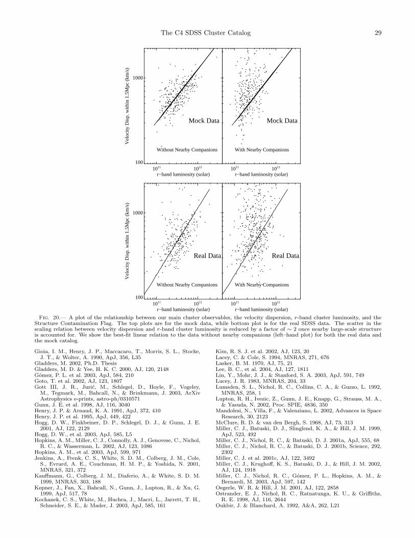
The C4 SDSS Cluster Catalog 29

1011 1012

r−band luminosity (solar)

100

1000

Vel

ocity

Dis

p. w

ithin

1.5

Mpc

(km

/s)

Without Nearby Companions

Mock Data

1011 1012

r−band luminosity (solar)

With Nearby Companions

Mock Data

1011 1012

r−band luminosity (solar)

100

1000

Vel

ocity

Dis

p. w

ithin

1.5

Mpc

(km

/s)

Without Nearby Companions

Real Data

1011 1012

r−band luminosity (solar)

With Nearby Companions

Real Data

Fig. 20.— A plot of the relationship between our main cluster observables, the velocity dispersion, r-band cluster luminosity, and theStructure Contamination Flag. The top plots are for the mock data, while bottom plot is for the real SDSS data. The scatter in thescaling relation between velocity dispersion and r-band cluster luminosity is reduced by a factor of ∼ 2 once nearby large-scale structureis accounted for. We show the best-fit linear relation to the data without nearby companions (left–hand plot) for both the real data andthe mock catalog.

Gioia, I. M., Henry, J. P., Maccacaro, T., Morris, S. L., Stocke,J. T., & Wolter, A. 1990, ApJ, 356, L35

Gladders, M. 2002, Ph.D. ThesisGladders, M. D. & Yee, H. K. C. 2000, AJ, 120, 2148Gomez, P. L. et al. 2003, ApJ, 584, 210Goto, T. et al. 2002, AJ, 123, 1807Gott III, J. R., Juric, M., Schlegel, D., Hoyle, F., Vogeley,

M., Tegmark, M., Bahcall, N., & Brinkmann, J. 2003, ArXivAstrophysics e-prints, astro-ph/0310571

Gunn, J. E. et al. 1998, AJ, 116, 3040Henry, J. P. & Arnaud, K. A. 1991, ApJ, 372, 410Henry, J. P. et al. 1995, ApJ, 449, 422Hogg, D. W., Finkbeiner, D. P., Schlegel, D. J., & Gunn, J. E.

2001, AJ, 122, 2129Hogg, D. W., et al. 2003, ApJ, 585, L5Hopkins, A. M., Miller, C. J., Connolly, A. J., Genovese, C., Nichol,

R. C., & Wasserman, L. 2002, AJ, 123, 1086Hopkins, A. M., et al. 2003, ApJ, 599, 971Jenkins, A., Frenk, C. S., White, S. D. M., Colberg, J. M., Cole,

S., Evrard, A. E., Couchman, H. M. P., & Yoshida, N. 2001,MNRAS, 321, 372

Kauffmann, G., Colberg, J. M., Diaferio, A., & White, S. D. M.1999, MNRAS, 303, 188

Kepner, J., Fan, X., Bahcall, N., Gunn, J., Lupton, R., & Xu, G.1999, ApJ, 517, 78

Kochanek, C. S., White, M., Huchra, J., Macri, L., Jarrett, T. H.,Schneider, S. E., & Mader, J. 2003, ApJ, 585, 161

Kim, R. S. J. et al. 2002, AJ, 123, 20Lacey, C. & Cole, S. 1994, MNRAS, 271, 676Lasker, B. M. 1970, AJ, 75, 21Lee, B. C., et al. 2004, AJ, 127, 1811Lin, Y., Mohr, J. J., & Stanford, S. A. 2003, ApJ, 591, 749Lucey, J. R. 1983, MNRAS, 204, 33Lumsden, S. L., Nichol, R. C., Collins, C. A., & Guzzo, L. 1992,

MNRAS, 258, 1Lupton, R. H., Ivezic, Z., Gunn, J. E., Knapp, G., Strauss, M. A.,

& Yasuda, N. 2002, Proc. SPIE, 4836, 350Mandolesi, N., Villa, F., & Valenziano, L. 2002, Advances in Space

Research, 30, 2123McClure, R. D. & van den Bergh, S. 1968, AJ, 73, 313Miller, C. J., Batuski, D. J., Slinglend, K. A., & Hill, J. M. 1999,

ApJ, 523, 492Miller, C. J., Nichol, R. C., & Batuski, D. J. 2001a, ApJ, 555, 68Miller, C. J., Nichol, R. C., & Batuski, D. J. 2001b, Science, 292,

2302Miller, C. J. et al. 2001c, AJ, 122, 3492Miller, C. J., Krughoff, K. S., Batuski, D. J., & Hill, J. M. 2002,

AJ, 124, 1918Miller, C. J., Nichol, R. C., Gomez, P. L., Hopkins, A. M., &

Bernardi, M. 2003, ApJ, 597, 142Oegerle, W. R. & Hill, J. M. 2001, AJ, 122, 2858Ostrander, E. J., Nichol, R. C., Ratnatunga, K. U., & Griffiths,

R. E. 1998, AJ, 116, 2644Oukbir, J. & Blanchard, A. 1992, A&A, 262, L21

30 Miller et al.

Oppenheimer, B. R., Helfand, D. J., & Gaidos, E. J. 1997, AJ, 113,2134

Perlmutter, S. & Schmidt, B. P. 2003, LNP Vol. 598: Supernovaeand Gamma-Ray Bursters, 195

Petrosian, V. 1976, ApJ, 209, L1Pier, J. R., Munn, J. A., Hindsley, R. B., Hennessy, G. S., Kent,

S. M., Lupton, R. H., & Ivezic, Z. 2003, AJ, 125, 1559Popesso, P., Bohringer, H., Brinkmann, J., Voges, W., & York,

D. G. 2004, A&A, 423, 449Postman, M., Lubin, L. M., Gunn, J. E., Oke, J. B., Hoessel, J. G.,

Schneider, D. P., & Christensen, J. A. 1996, AJ, 111, 615Postman, M., Lauer, T. R., Oegerle, W., & Donahue, M. 2002,

ApJ, 579, 93Reichart, D. E., Nichol, R. C., Castander, F. J., Burke, D. J.,

Romer, A. K., Holden, B. P., Collins, C. A., & Ulmer, M. P.1999, ApJ, 518, 521

Romer, A. K. et al. 2000, ApJS, 126, 209Romer, A. K. & et al. 2004, Clusters of Galaxies: Probes of

Cosmological Structure and Galaxy EvolutionSand, D. J., Treu, T., & Ellis, R. S. 2002, ApJ, 574, L129Schlegel, D. J., Finkbeiner, D. P., & Davis, M. 1998, ApJ, 500, 525Scranton, R., et al. 2002, ApJ, 579, 48Smith, J. A. et al. 2002, AJ, 123, 2121Sochting, I. K., Clowes, R. G., & Campusano, L. E. 2002, MNRAS,

331, 569Stoughton, C. et al. 2002, AJ, 123, 485Strauss, M. A. et al. 2002, AJ, 124, 1810Sutherland, W. 1988, MNRAS, 234, 159Tully, R. B., Mould, J. R., & Aaronson, M. 1982, ApJ, 257, 527Viana, P. T. P. & Liddle, A. R. 1996, MNRAS, 281, 323

Vikhlinin, A., McNamara, B. R., Forman, W., Jones, C., Quintana,H., & Hornstrup, A. 1998, ApJ, 502, 558

Visvanathan, N. & Sandage, A. 1977, ApJ, 216, 214Voges, W., et al. 1999, A&A, 349, 389Wechsler, R. H. 2004, Clusters of Galaxies: Probes of Cosmological

Structure and Galaxy EvolutionWegner, G., Colless, M., Baggley, G., Davies, R. L., Bertschinger,

E., Burstein, D., McMahan, R. K., & Saglia, R. P. 1996, ApJS,106, 1

Wei, J. Y., Xu, D. W., Dong, X. Y., & Hu, J. Y. 1999, A&AS, 139,575

White, R. A., Bliton, M., Bhavsar, S. P., Bornmann, P., Burns,J. O., Ledlow, M. J., & Loken, C. 1999, AJ, 118, 2014

White, M. 2002, ApJS, 143, 241Wittman, D. 2002, LNP Vol. 608: Gravitational Lensing: An

Astrophysical Tool, 55Yang, X., Mo, H. J., Jing, Y. P., van den Bosch, F. C., & Chu, Y.

2004, MNRAS, 350, 1153Yee, H. and Ellingson, E. 2003, ApJ, 585, 215York, D. G. et al. 2000, AJ, 120, 1579Zehavi, I., et al. 2002, ApJ, 571, 172Zwicky, F. 1952, PASP, 64, 247Zwicky, F., Herzog, E., & Wild, P. 1961, CGCG1, 0Zwicky, F. & Herzog, E. 1963, CGCG2, 0Zwicky, F., Karpowicz, M., & Kowal, C. T. 1965, CGCG5, 0Zwicky, F. & Herzog, E. 1966, CGCG3, 0Zwicky, F. & Herzog, E. 1968a, CGCG4,0Zwicky, F. & Kowal, C. T. 1968b, CGCG6, 0

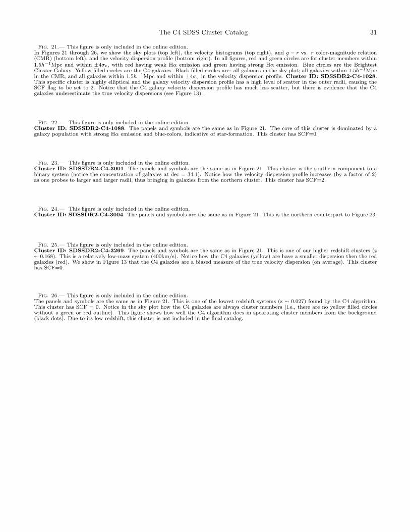
The C4 SDSS Cluster Catalog 31

Fig. 21.— This figure is only included in the online edition.In Figures 21 through 26, we show the sky plots (top left), the velocity histograms (top right), and g − r vs. r color-magnitude relation(CMR) (bottom left), and the velocity dispersion profile (bottom right). In all figures, red and green circles are for cluster members within1.5h−1Mpc and within ±4σv, with red having weak Hα emission and green having strong Hα emission. Blue circles are the BrightestCluster Galaxy. Yellow filled circles are the C4 galaxies. Black filled circles are: all galaxies in the sky plot; all galaxies within 1.5h−1Mpcin the CMR; and all galaxies within 1.5h−1Mpc and within ±4σv in the velocity dispersion profile. Cluster ID: SDSSDR2-C4-1028.This specific cluster is highly elliptical and the galaxy velocity dispersion profile has a high level of scatter in the outer radii, causing theSCF flag to be set to 2. Notice that the C4 galaxy velocity dispersion profile has much less scatter, but there is evidence that the C4galaxies underestimate the true velocity dispersions (see Figure 13).

Fig. 22.— This figure is only included in the online edition.Cluster ID: SDSSDR2-C4-1088. The panels and symbols are the same as in Figure 21. The core of this cluster is dominated by agalaxy population with strong Hα emission and blue-colors, indicative of star-formation. This cluster has SCF=0.

Fig. 23.— This figure is only included in the online edition.Cluster ID: SDSSDR2-C4-3001. The panels and symbols are the same as in Figure 21. This cluster is the southern component to abinary system (notice the concentration of galaxies at dec = 34.1). Notice how the velocity dispersion profile increases (by a factor of 2)as one probes to larger and larger radii, thus bringing in galaxies from the northern cluster. This cluster has SCF=2

Fig. 24.— This figure is only included in the online edition.Cluster ID: SDSSDR2-C4-3004. The panels and symbols are the same as in Figure 21. This is the northern counterpart to Figure 23.

Fig. 25.— This figure is only included in the online edition.Cluster ID: SDSSDR2-C4-3269. The panels and symbols are the same as in Figure 21. This is one of our higher redshift clusters (z∼ 0.168). This is a relatively low-mass system (400km/s). Notice how the C4 galaxies (yellow) are have a smaller dispersion then the redgalaxies (red). We show in Figure 13 that the C4 galaxies are a biased measure of the true velocity dispersion (on average). This clusterhas SCF=0.

Fig. 26.— This figure is only included in the online edition.The panels and symbols are the same as in Figure 21. This is one of the lowest redshift systems (z ∼ 0.027) found by the C4 algorithm.This cluster has SCF = 0. Notice in the sky plot how the C4 galaxies are always cluster members (i.e., there are no yellow filled circleswithout a green or red outline). This figure shows how well the C4 algorithm does in spearating cluster members from the background(black dots). Due to its low redshift, this cluster is not included in the final catalog.

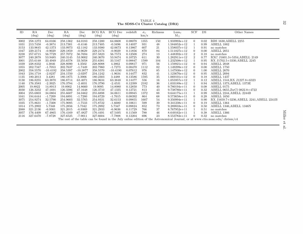
32

Miller

etal.

TABLE 4The SDSS-C4 Cluster Catalog (DR2)

ID RA Dec RA Dec BCG RA BCG Dec redshift σv Richness Lumr SCF DS Other Names(deg) (deg) (deg) (deg) (deg) (deg) km/s M⊙

3002 258.1272 64.0166 258.1362 64.0183 258.1200 64.0608 0.08078 1355 150 1.933993e+12 0 0.02 RBS 1630,ABELL 22551031 213.7458 -0.3874 213.7301 -0.4146 213.7405 -0.3496 0.14037 931 48 1.584852e+12 1 0.99 ABELL 18823153 133.9645 42.1373 133.9973 42.1182 133.9380 42.0673 0.13867 607 21 1.558037e+12 1 0.91 no matches1047 229.2174 -0.9029 229.1859 -0.9629 229.2174 -0.9029 0.11856 870 84 1.511027e+12 0 0.00 ABELL 20513238 257.6715 56.7729 257.7072 56.7694 257.5823 56.7573 0.12508 274 13 1.448392e+12 2 0.18 no matches3077 240.2678 53.9485 240.3145 53.9002 240.3670 53.9474 0.10725 611 30 1.282911e+12 2 0.77 RXC J1601.3+5354,ABELL 21493001 255.6148 33.4949 255.6578 33.5058 255.6381 33.5167 0.08847 1599 104 1.232508e+12 1 0.95 RX J1702.5+3330,ABELL 22451039 228.8332 4.3846 228.8090 4.3502 228.8088 4.3862 0.09817 971 56 1.159921e+12 0 0.94 ABELL 20481055 202.7347 -1.7053 202.7637 -1.7449 202.7960 -1.7273 0.08470 1112 82 1.149299e+12 0 0.00 ABELL 17502002 358.5570 -10.4192 358.5397 -10.3877 358.5570 -10.4190 0.07612 976 85 1.147930e+12 0 1.00 ABELL 26701043 234.1718 -2.0237 234.1550 -2.0297 234.1242 -1.9634 0.14477 832 41 1.123676e+12 0 0.95 ABELL 20941135 180.2013 3.4281 180.1875 3.3906 180.2303 3.4488 0.13586 1595 35 1.069101e+12 0 0.18 ABELL 14373130 186.8255 63.3870 186.8714 63.4071 186.9634 63.3848 0.14477 556 16 1.055957e+12 1 0.12 ABELL 1544,RX J1227.8+63231140 176.3583 -2.3925 176.3784 -2.4031 176.3790 -2.4531 0.12399 2182 36 1.033189e+12 1 0.94 ABELL 1373,ABELL 1373E2005 19.8822 14.8913 19.8902 14.8660 19.9095 14.8980 0.12850 773 40 9.780194e+11 0 0.08 ABELL 01753030 126.3232 47.1691 126.3386 47.1648 126.3710 47.1335 0.12721 813 43 9.738780e+11 0 0.32 ABELL 0655,ZwCl 0822.8+47223004 255.6803 34.0804 255.6607 34.0462 255.6898 34.0611 0.09945 1372 88 9.644175e+11 1 0.99 ABELL 2244,ABELL 2244B1041 194.6444 -1.7209 194.6891 -1.7280 194.6729 -1.7615 0.08392 864 68 9.573658e+11 0 0.28 ABELL 16503075 254.9274 32.5790 254.9603 32.5765 254.9331 32.6153 0.09855 1607 54 9.350994e+11 1 0.90 RX J1659.7+3236,ABELL 2241,ABELL 2241B1035 175.8631 -1.7308 175.9095 -1.7533 175.8722 -1.6680 0.10611 599 39 9.341238e+11 0 0.19 ABELL 13641014 175.2992 5.7348 175.2856 5.7342 175.2992 5.7347 0.09824 852 73 9.289833e+11 0 0.50 ABELL 1346,ABELL 1346N2088 321.2136 -6.9301 321.2015 -6.9369 321.2933 -6.9636 0.11729 766 37 8.767952e+11 1 0.51 no matches3057 176.4409 67.4865 176.4169 67.4827 176.4491 67.5495 0.11569 788 46 8.649162e+11 1 0.38 ABELL 13662116 327.6470 -7.8728 327.6525 -7.9011 327.6604 -7.7888 0.12204 696 23 8.553782e+11 0 0.32 no matches

The rest of the table can be found in the July online edition of the Astronomical Journal, or at www.ctio.noao.edu/ chrism/c4