arX

iv:a

stro

-ph/

0703

475v

1 1

9 M

ar 2

007

– 1 –

Efficient intra- and inter-night linking

of asteroid detections using kd-trees

27 manuscript pages

14 figures

7 tables

Keywords: Asteroids

– 2 –

Running Head:

Efficient linking of asteroid detections

Editorial Correspondence and Proofs:

Robert Jedicke

Institute for Astronomy

University of Hawaii

Honolulu, HI, 96822

Tel: 808.956.9841

Fax: 808.988.8972

E-mail: jedicke@ifa.hawaii.edu

Efficient intra- and inter-night linking

of asteroid detections using kd-trees

Jeremy Kubica1†, Larry Denneau2, Tommy Grav2, James Heasley2, Robert Jedicke2,

Joseph Masiero2, Andrea Milani3, Andrew Moore1†, David Tholen2, Richard J. Wainscoat2

1The Robotics Institute, 5000 Forbes Avenue, Pittsburgh, PA, 15213-3890

2Institute for Astronomy, University of Hawaii, Honolulu, HI, 96822

3 Dipartimento di Matematica, Via Buonarroti 2, 56127 Pisa, Italy

† now at Google, Collaborative Innovation Center, 4720 Forbes Avenue, Pittsburgh, PA,

15213

March 12, 2018

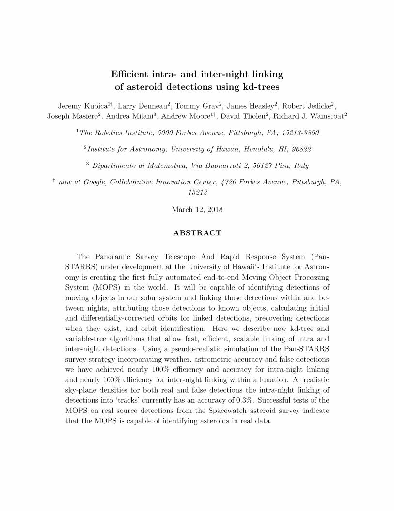
ABSTRACT

The Panoramic Survey Telescope And Rapid Response System (Pan-

STARRS) under development at the University of Hawaii’s Institute for Astron-

omy is creating the first fully automated end-to-end Moving Object Processing

System (MOPS) in the world. It will be capable of identifying detections of

moving objects in our solar system and linking those detections within and be-

tween nights, attributing those detections to known objects, calculating initial

and differentially-corrected orbits for linked detections, precovering detections

when they exist, and orbit identification. Here we describe new kd-tree and

variable-tree algorithms that allow fast, efficient, scalable linking of intra and

inter-night detections. Using a pseudo-realistic simulation of the Pan-STARRS

survey strategy incorporating weather, astrometric accuracy and false detections

we have achieved nearly 100% efficiency and accuracy for intra-night linking

and nearly 100% efficiency for inter-night linking within a lunation. At realistic

sky-plane densities for both real and false detections the intra-night linking of

detections into ‘tracks’ currently has an accuracy of 0.3%. Successful tests of the

MOPS on real source detections from the Spacewatch asteroid survey indicate

that the MOPS is capable of identifying asteroids in real data.

– 4 –

1. Introduction

The next generation of wide-field sky surveys will be capable of discovering as many solar

system objects in one lunation as are currently known. Their unprecedented discovery rate

coupled with their deep limiting magnitudes will make targeted astrometric and photometric

followup observations impossible for the vast majority of objects. Thus, it is necessary that

the new search programs employ survey strategies that reacquire multiple observations of the

same objects within a lunation (a lunar synodic period). Furthermore, these facilities would

tax the current capability of the International Astronomical Union’s Minor Planet Center

(MPC), the clearing house for observations of the solar system’s small bodies, for linking

the detections and orbit determination. The only solution is that the surveys must provide

the capability themselves and then provide the MPC with pre-linked, vetted detections over

multiple nights. Simplistic linking algorithms for those detections scale like the square of the

sky-plane density (ρ) and, at the high densities expected for the next generation surveys,

the linking procedure could dominate the processing time. This work presents algorithms

to solve the problem that are fast, efficient, accurate and scale as O(ρ log ρ). We test our

algorithms on pseudo-realistic simulations.

The history of asteroid orbit determination is mathematically rich. It all began with

the visual discovery of Ceres by Giuseppe Piazzi in 1801 and subsequent theory of orbit

determination by Gauss (1809). At that time new techniques were developed to handle

the orbit determination from a short arc of observations and the ephemeris errors on the

observations of Ceres were many arcseconds. Two hundred years later absolute astrometric

residuals are about an order of magnitude better and the next generation surveys promise

to reduce those residuals for bright asteroids another order of magnitude.

As of 2006 August 6 there were a total of 338,470 asteroids in the astorb database

(Bowell et al. 1994) and over 20K asteroid observations are reported daily to the Minor

Planet Center. As new observations of previously known asteroids are identified their orbital

elements are automatically updated. Furthermore, new observations of asteroids that were

unknown are linked together and their orbits are calculated quickly and automatically by

digital computers.

The discovery rate of asteroids and comets has climbed dramatically in the past decade

(for an overview of current asteroid search programs see Stokes et al. (2002)) due to the

advent of new technologies like the CCD camera and because of NASA’s Congressional

mandate to search for Near Earth Objects (NEO) larger than 1km in diameter (Morrison

1992). The mandate to identify 90% of NEOs in this size range will most likely be achieved

shortly after the 2008 deadline (Jedicke et al. 2003).

– 5 –

Asteroids (and often comets) are usually identified by their apparent motion against

background stars in an image during the time between three or more exposures separated

in time by tens of minutes. All existant surveys have relied on the nearly linear motion of

the objects on the sky during the short time between exposures to distinguish between real

objects and random alignments of false detections (noise). Some historical and contemporary

surveys identify or check their observations of moving objects by eye.

As the discovery rate and the limiting magnitude of the surveys has increased the sky-

plane density of asteroids has increased and, with it, the opportunity for false identifications

and linkages. This explosion in the number of reported observations to the MPC has gen-

erated a corresponding theoretical examination of the techniques used in linking new obser-

vations and fitting orbits (e.g. Milani et al. 2005; Granvik & Muinonen 2005; Kristensen

2004, 2002; Virtanen et al. 2001; Kristensen 1992; Marsden 1985). These problems, as well

as that of attribution (identifying observations with known objects), orbit identification (re-

alizing that multiple instances of an object’s orbit appear in a database), and precovering

observations (identifying earlier detections of an object in a database), are described by Mi-

lani et al. in a series of articles (Milani et al. 2001, 2000; Milani 1999; Milani & Valsecchi

1999).

This work describes new algorithms, and the testing framework developed to measure

their efficiency and accuracy, for intra and inter-night linking of asteroid detections. The

algorithms work well in simulations of the performance of the next generation sky surveys.

2. Pan-STARRS

Spurred by the 2001 decadal review (McKee & Taylor et al. 2001) a new generation of

all-sky surveys are expected to commence operations within the next ten years. These new

surveys will take advantage of the latest developments in optical designs (e.g. to produce

large, flat fields of view) and CCD technology (e.g. extremely fast readout) to survey the

sky faster and deeper than ever before.

The first of the next generation surveys to image the sky will be the Panoramic Sur-

vey Telescope And Rapid Response System (Pan-STARRS, Hodapp et al. 2004) located in

Hawaii. Pan-STARRS will be composed of four 1.8m diameter telescopes each with its own

1.44 Gpix camera (0.3′′/pixel). Images from each of the four cameras will be combined to-

gether electronically. The cameras will use an innovative new CCD technology composed of

Orthogonal Transfer Arrays (OTA, Tonry et al. 1997) that allow charge to be moved on the

CCD in both the x and y directions in real time at ∼30 Hz to compensate for image motion

– 6 –

due to the atmosphere or any tracking problems. In effect, the system produces a tip-tilt

corrective optics on-chip rather than with the secondary and it is able to achieve superior

seeing over the entire ∼7 deg2 field-of-view rather than just within the small isoplanatic an-

gle in the center of the field. A prototype system (PS1) located on the summit of Haleakala,

HI, saw first light in the summer of 2006 and will begin science operations in the summer of

2007.

One of the primary scientific goals of the Pan-STARRS survey is to identify 90% of

all potentially hazardous objects larger than 300m diameter within its ten year operational

lifetime. In the process it will identify about 10 million other solar system objects. It is

expected to reach R ∼ 24 at 5-sigma in 30sec exposures at which level the sky-plane density

of asteroids will be about 250/deg2 on the ecliptic. This is also the predicted density of false

5-sigma detections in the image. Thus, the ratio of false:real detections at 5-sigma is equal

to unity on the ecliptic and increases dramatically off the ecliptic. Given enough computing

power and/or time it is, in principle, possible to link individual detections together on

separate nights of observation. A priori distributions of asteroid velocities and accelerations

at any sky location could be used to intelligently link detections on separate nights and

then fit orbits to them to select those that represent observations of objects. (Note that we

distinguish between a detection, which is a set of pixels on an image with elevated signal

relative to the background, and an observation which is a detection associated with a real

object.) This method has not yet been used in practice because of the combinatorics of the

problem as the limiting magnitude of the system is approached and the number of real and

false detections increases dramatically. It is almost certain that this technique will require 4

nights on which each object was detected in order to determine orbits with good fidelity.

As mentioned above, the typical contemporary asteroid survey obtains ≥3 observations

of an asteroid within a short period of time on a night. When these observations are sub-

mitted to the MPC there is high probability that each set of detections corresponds to a real

object. The MPC’s responsibility is to link these detections to known objects or to other

new detections of the same object. Many of the contemporary and all the historical asteroid

surveys identified NEOs through their anomalous rates of motion relative to other objects

in or near the field of view (Jedicke 1996).

There are two main problems with this mode of operation for the next generation

surveys. First, in order to guarantee that reported sets of detections correspond to real

objects, surveys require ≥3 detections on a night which dramatically limits the system’s sky

coverage; e.g. a system that obtains only 2 detections/night can cover 50% more sky, and

obtain 50% more detections than a survey requiring 3 detections/night. Second, follow-up of

NEO detections for the contemporary surveys is typically accomplished by the survey itself

– 7 –

or by other professional surveying systems. Since the first next generation survey (at least)

will not have the luxury of any other existing system being able to recover newly discovered

objects, the survey must obtain its own follow-up.

The Pan-STARRS system will most likely obtain just 2 images per night of each solar

system survey field but re-image the field 3 or 4 times within a lunation. Two images are used

each night in order to distinguish between false and real detections and separate stationary

and moving transient objects. It also has the benefit of providing a small motion vector

for each possible observation. Obtaining the same object a few more times within the next

two weeks provides both recovery of the objects and more nights of observations with which

to calculate an orbit and verify the reality of each set of detections. Since it is (currently)

required that detections reported to the MPC have a high probability of being legitimate

observations, Pan-STARRS will only report those detections to the MPC that are linked

across nights into real orbits. Thus, Pan-STARRS must develop the capability of linking

detections across nights into real orbits. If the MPC relaxes the condition on the accuracy

of linked detections then Pan-STARRS will report everything that is available.

The responsibility for intra-night (within a night) and inter-night (between many nights)

linking of detections (as well as attributing, precovering, orbit determination and identifica-

tionm, etc.) rests with Pan-STARRS’s Moving Object Processing System (MOPS).

3. Pan-STARRS Moving Object Processing System (MOPS)

Images from the cameras on each of the four Pan-STARRS telescopes (for the Pan-

STARRS-1 system only a single camera and telescope will be in operation) are first passed

through the Image Processing Pipeline (IPP) that aligns, warps, removes cosmic rays, etc.,

and digitally combines them into a single master image. Many master images are combined

together to create a high S/N static-sky images that is subtracted from the current master

image to obtain a difference image containing only transient sources (stationary and moving)

and noise (false detections). The difference image is then searched for sources consistent with

being asteroids (both nearly stationary and moving fast enough to trail) and also for comets.

Pairs of difference images separated by a Transient Time Interval (TTI) of about 15-30

minutes (the time separation is still to be determined and may vary with sky-plane location)

are analyzed in the same manner. A list of all the identified sources in both images along

with their characteristics (time, trail length, axis orientation, flux, etc.) is then passed to

the MOPS. The software and algorithms described herein are expected to be applicable to

both Pan-STARRS-4 and Pan-STARRS-1 and the tests described herein are performed at

asteroid sky-plane densities (i.e. limiting magnitude) expected for the four telescope system.

– 8 –

The MOPS will;

• link intra-night detections into probable observations (tracklets),

• attribute tracklets to known objects,

• link inter-night detections into possible objects (tracks),

• perform an initial orbit determination (IOD) to select tracks that are likely to be real

objects,

• perform a differential correction to the orbit determination (OD) to obtain a derived

orbit for the track,

• identify whether an earlier derived orbit is identical to the current orbit,

• seek precoveries in all earlier images of the derived object,

• and determine its operational efficiency and accuracy in nearly real time using a syn-

thetic solar system model.

The results described herein only describe the algorithms and efficiency for the first and

third steps, the intra-night and inter-night linking of detections. The performance of the

MOPS for the other aspects of its operation will be described in future papers.

At 5-sigma (or r ∼ 24mag) we expect about 250 false detections/deg2 (Kaiser 2004)

or about 1750 false detections per image at any position on the sky. To the same S/N we

also expect a maximum sky-plane density of asteroids on the ecliptic of about 250/deg2

(Gladman et al. 2006; Masiero et al. 2006; Yoshida et al. 2003) but this number decreases

dramatically off the ecliptic. At 3-sigma the false detection rate will be about 100× higher

with only an increase of about 1.4× in the number of real detections. It is clear from these

ratios that the difficulty of identifying asteroid observations increases substantially as we

push the limiting operational S/N into the noise. The S/N at which the Pan-STARRS

MOPS will operate will be determined when the actual operational characteristics of the

system are known. For this work we assume a 5-sigma cutoff corresponding to r ∼ 24mag

for the four telescope Pan-STARRS facility.

The first step in the MOPS is to identify sets of detections in images within a night that

are spatially close and therefore likely to be observations of a real object. We call these sets

of detections tracklets. The MOPS also uses trailing information in the form of the length

and orientation of each detection to further constrain the intra-night linking problem - only

those detections that have the expected trail length and orientation given their separation

– 9 –

in time and space are combined into tracklets. We will demonstrate below that our process

is almost 100% efficient at identifying tracklets with an accuracy in the range of 85-90% (see

table 1).

The second MOPS step is the inter-night linking of tracklets into sets that we call tracks.

In operations this step is followed by IOD and OD to select only those tracks that are valid

orbits. We will show below that at the expected sky-plane density of real and false detections

the set of realized tracks are mostly false. But after IOD and OD we are left with a nearly

pure sample of actual orbits. The key is to use the track formation process to reduce the

number of false tracks to a sufficiently small number that it is feasible to calculate orbits for

all tracks within the required time frame.

The difficulty in intra- and inter-night linking of detections is combinatoric and in-

creases like ρ2, where ρ is the number of detections/deg2, if a brute-force approach is

taken in linking the detections. A few sophisticated techniques have been proposed (e.g.

Granvik & Muinonen 2005; Milani et al. 2005) to deal with these problems. We report

here on our success with a linking algorithm that makes use of a clever data structure

(known as a kd-tree) to convert the combinatoric problem in both cases into one that in-

creases instead like ρ log ρ. In this manner we can explore and reject many possible linkages

without resorting to sophisticated and time consuming orbit determination techniques and

thereby increase the speed with which we can manage the large number of detections (false

and real) from the next generation surveys.

4. Solar System Model

To verify that our linking algorithms are efficient we require a model of the various

populations of small bodies in our solar system that could possibly reach r ∼ 24.5. This

simulation requires realistic orbits rather than simply the objects’ spatial distribution. These

requirements forced us into developing our own Solar System Model (SSM) rather than

adopting Tedesco et al. (2005)’s Statistical Asteroid Model (SAM) for main belt asteroids,

though we were motivated by some of the techniques developed for the SAM.

Our SSM will be discussed in detail by Denneau et al. (2006a) and only briefly here (also

Milani et al. 2006). For the purpose of testing the MOPS we have developed a preliminary

model of many populations of objects in our solar system and beyond including nearly 11

million small bodies:

• Near Earth Objects (NEO) (including objects entirely interior to the Earth’s orbit)

– 10 –

• Main Belt Objects (MBO)

• Jupiter trojans and trojans of all other planets

• Centaurs (CEN)

• Jupiter Family, Halley-type and Oort Cloud comets (COM)

• Trans-Neptunian objects (TNO) - classical, resonant, scattered and extended scattered

disk.

The details of the model are not critical to interpreting the work reported here. In

general, we have a preliminary model of different small body populations in the solar system

(and some populations that have not been discovered) that mimic the real objects at different

levels of fidelity in each of the following properties:

• orbit distribution

• absolute magnitude (H), size and albedo distribution

• shapes modelled as tri-axial ellipsoids

• rotation rates

• pole orientations

For the simulations described here we simply used the absolute magnitude and standard for-

mulae (Bowell et al. 1989) for converting to apparent magnitudes rather than incorporating

the shape, rotation rate and pole orientation.

The input orbit distributions for the NEOs (Bottke et al. 2002) and CENs (Jedicke & Herron

1997) have a pedigree traceable to published studies while the MBOs mimic the large statis-

tics of the nearly complete MBO population (for H < 14.5) (Jedicke et al. 2002). For the

moment, the input orbit distributions for the other populations are based only on the ob-

served rather than the debiased populations. In all cases we generated a full suite of objects

that might achieve r < 24.5 (the expected Pan-STARRS-4 limiting magnitude) at some time

in the next ten years.

The absolute magnitude distributions were generated according to corrected H distri-

butions where available (NEO - Bottke et al. (2002), MBO - Jedicke et al. (2002), CEN -

Jedicke & Herron (1997), TRO - Jewitt et al. (2000), TNO - Bernstein et al. (2004), SDO

- Elliot et al. (2005)). For all types of comets the absolute magnitude distribution was

– 11 –

simply the observed distribution extended to smaller sizes in a natural manner. It is our

intention to improve this model for comets in the final solar system model implement for

MOPS.

5. Survey Simulation

Many researchers have modelled asteroid surveys in an attempt to predict the perfor-

mance of a particular system (e.g. Raymond et al. 2004; Mignard 2002). Others have mod-

elled generic survey systems in order to elucidate more general principles (e.g. Jedicke et al.

2003; Harris 1998). For instance, in the case of discovering NEOs, Bowell & Muinonen

(1994) and Harris (1998) showed that it is more important to cover more sky than it is to

go to fainter limiting magnitudes in a smaller area. These earlier simulations had a wide

range of fidelity to realism with some merely postulating that the entire sky would be covered

in a night.

The final mode of solar system surveying for Pan-STARRS will be under study until

regular asteroid surveying begins in earnest. Even then, we believe that a regular review of

the survey strategy will be necessary in an attempt to maximize the system efficiency. The

simulation of the survey implemented here is our first-order vision that incorporates many of

the most important aspects of an efficient and realistic survey that has as its highest priority

the identification of sub-km Potentially Hazardous Objects (PHO). A full discussion of the

survey simulation and its impact on the MOPS asteroid discovery rates is in preparation

(Denneau et al. 2006b).

With PHOs in mind we place a high emphasis on covering the ‘sweet-spots’, the sky

at small solar elongation and small ecliptic latitude where the sky-plane density of PHOs

at Pan-STARRS’s limiting magnitude is expected to be highest (Chesley & Spahr 2004).

We take advantage of the fact that asteroids tend to be brighter near the anti-solar point

and attempt to identify high inclination or nearby objects surveying a wide area in both

longitude and latitude near opposition.

For the purpose of this work consider an ecliptic longitude (λ′, opposition longitude) and

latitude (β) system centered on the opposition point. e.g. opposition is always at (0, 0). In

this reference frame the solar system survey is defined by the two sweet spots with |β| < 10◦,

−120◦ < λ′ < −90◦ or +90◦ < λ′ < +120◦ and also the opposition region with |λ′| < 30◦

and |β| < 40◦ totaling about 5500 deg2. To simplify our simulation we assumed that the

Pan-STARRS fields are square and of an area about equal to the final expected camera field.

Figure 1 shows the distribution of equal area field centers on the sky in the sweet-spots and

– 12 –

opposition regions. There are 660 fields in the opposition region and 84 in each of the sweet-

spots corresponding to field coverage of about 4,356 deg2 and 1108 deg2 (in both sweet-spots)

respectively. Each Pan-STARRS field covers about 7 deg2 so this simulation allows for some

moderate overlap between adjacent fields.

It is important to note that this scanning pattern (and the one likely to be adopted

for Pan-STARRS solar system survey operations) avoids the (Main Belt) ’stationary spots’

about 3.5 hours (∼ 50◦) from opposition. The stationary spots are regions where apparent

asteroid motion along the ecliptic may briefly drop to zero. The more distant the asteroid

population the greater the distance from opposition at which the objects become ’stationary’.

For intance, TNOs are stationary fully 80◦ from opposition - nearly in what we refer to as

the sweet-spots. Asteroid paths on the sky can even form closed loops far from opposition

that might cause difficulty for the linking algorithm desribed herein.

Moving objects will drift out of any fixed region on the sky. Even a fixed-size region

that moves at the mean rate of motion of moving objects in the field will lose objects near

its edge. One solution is to expand the size of the region with time. Another solution is to

ensure that the region translates at a rate equal to the mean rate of motion of the objects

of primary interest in the region.

We have used our solar system model (§4) to determine the apparent rate of motion of

NEOs with r < 24mag in the three survey regions. The sweet spots are small enough in

ecliptic longitude extent (30◦) that we included all NEOs in those regions and found that they

are moving at mean rates of dβ/dt = 0◦/day (as expected from symmetry) and prograde at

dλ′/dt ∼ +0.65◦/day. The opposition region covers a much wider range in ecliptic longitude

and we are only in danger of losing objects that are near its eastern and western edges.

Thus, only those NEOs within 15◦ of the eastern or western edge of the region were used to

determine that they are moving retrograde at a mean rate of dλ′/dt ∼ −0.30◦/day.

For the purpose of this work we have assumed that the solar system survey requires

imaging of each field within a region three (3) times per lunation with a mininum spacing

of four (4) nights between any successive visit to each field. While this scenario is suitable

for this simulation we have evidence that another night of observation, especially in the

sweet-spots, will be necessary to resolve degenerate multiple orbit solutions. When running

the simulation we have assumed that a random 25% of nights are entirely clouded out while

the remaining 75% are entirely clear. This results in a variable number of nights between

visits in a lunation.

The algorithm for scheduling the fields within the regions is described below. For the

purpose of developing the inter-night field scheduler it was convenient to think in terms of

– 13 –

scheduling nights with respect to full moon (FM +N = Full Moon plus N nights). Evening

and morning sweet spots may be acquired on the same night but the opposition region was

impossible to schedule in its entirety on a single night. We divided the opposition region

into northern and southern ecliptic latitudes that need to be acquired on separate nights

and may not be imaged on nights on which a sweet spot is acquired (sweet spots also have

higher priority).

5.1. Evening sweet spot

Objects in the evening sweet spot are being overtaken by the Sun. The first opportunity

to visit the ESS is just after full moon (FM + 4 days), when the waning moon is no longer

in the bright sky after astronomical twilight ends. The last opportunity to catch the ESS is

a few days after new moon (FM +18 days) before the young moon enters the evening sweet

spot.

When scheduling surveying in the ESS it is impossible (due to weather or the other

Pan-STARRS science survey requirements) to predict what night will be the actual last

night of observation. Thus, on the first possible night of surveying in the ESS we assume

the worst case scenario that the last possible night will be the last opportunity to survey the

same region at FM +18 days. The last night then defines the ESS region and we then work

backwards from that location at a rate of dλ/dt = +0.65◦/day to determine the location of

the ESS on any of the previous nights on which it is actually acquired.

5.2. Opposition

Scheduling of the opposition regions is constrained by the moon appearing in those

regions when it is full. For both regions we have assumed that the first day it is possible to

acquire these regions is at FM + 7 days and the last is at FM + 21 days.

When scheduling the opposition regions we assume that the second night will be acquired

at new moon and define the actual field locations on a specific night by translating the region

at a rate of dλ/dt = −0.3◦/day.

– 14 –

5.3. Morning sweet spot

Objects in the morning sweet spot are also heading towards the Sun but they have

many months until they pass behind it because the Sun is moving away from them faster

than they approach it. Thus, the location of NEOs in the area of the MSS move away from

the horizon with time and the sky-plane location of NEOs improves with time as a lunation

progresses. Surveying in the MSS may start just before new moon (FM + 10 days) and is

possible until the just-before-full moon enters the morning sky (FM + 24).

For scheduling the MSS region we simply survey the optimal MSS region on the first

possible day that it can actually be surveyed and translate the region by dλ/dt = +0.65◦/day

to determine the location of the MSS on subsequent nights on which it is acquired.

5.4. Nightly scheduling of fields

Once the fields for a specific night have been selected they need to be scheduled for that

night taking into account a wide range of system parameters and other factors. Pan-STARRS

will eventually employ a dynamic telescope scheduler that takes into account hundreds of

relevant factors. While the Pan-STARRS telescope scheduler is being developed, for testing

purposes the MOPS has adopted TAO (Tools for Automated Observing, Paulo Holvorcem,

http://pan-starrs.ifa.hawaii.edu/project/MOPS/TAO/html/readme.html). TAO is a macro-

scheduler and as such it attempts to schedule all fields on a single night as efficiently as

possible. There are far too many TAO configuration parameters to discuss each in detail

here. Several important configuration parameters are:

• Number of images of each target = 2

• sky-plane location

Preferring low air mass due to poorer seeing, higher extinction and increased sky

background at lower elevations..

• field priority

• intra-night cadence requirements

15min between visits to the same field on each night. The standard time between

exposures on the same night is known as a Transient Time Interval or TTI. There is a

50% tolerance on the actual scheduling.

• inter-night cadence requirements

No less than 3 nights between visits in a lunation.

– 15 –

• exposure time = 30sec

• read out time = 5sec

• telescope slew rate = 5◦/sec

• time of night = 5◦/sec

• azimuthally dependent altitude limits = 20◦ (∼2.85 airmasses)

• cloud cover

• seeing conditions

• Moon avoidance angle at full moon = 45◦ (scales with phase)

• Min/Max Sun Altitude = -15◦

Intermediate between nautical and astronomical twilight.

We ran the scheduler for ten years of synthetic surveying. The scheduling efficiency for

the solar system fields is essentially 100% for those fields that are well above the minimum

altitude (some of the most southern opposition fields are always below the altitude limit and

some of the sweet spot fields may also be unavailable at certain times of the year). Due to

‘weather’ some of the regions were not covered 3 times in a lunation.

Figure 2 shows the distribution of field locations in altitude vs. azimuth separately for

the sweet spots and opposition regions over the ten year survey. The sweet spots are typically

obtained between 20◦ and 70◦ altitude and 60◦ < |azimuth| < 160◦. The most likely altitude

is near 40◦ or about 1.7 airmasses. For the opposition regions note the predominance of

fields scheduled near ±180◦ and close to 0◦ - on or near the meridian when the fields are at

their highest possible altitude (lowest possible airmass).

6. Simulating detections

Given the survey simulation (§5) we generate accurate n-body ephemerides and pho-

tometry for the synthetic solar system objects (§4) that appear in each field of view. The

astrometric and photometric accuracy expected by Pan-STARRS is better than existing as-

teroid surveys. At r ∼ 24mag we expect astrometric error to be about 0.1′′ and a photometric

error of about 0.35mag. For brighter objects these errors will be considerably smaller.

The linking method described herein is independent of the detection’s apparent magni-

tude except for the requirement that the detection be above the limiting magnitude of the

– 16 –

system (to simulate the expected sky-plane density of asteroids). However, in the interest of

completeness, and since modern orbit determination software can utilize an estimate of the

S/N , we generate a pseudo-realistic magnitude and S/N for synthetic detections.

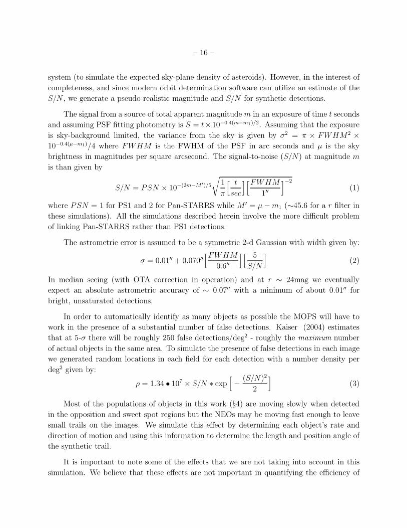
The signal from a source of total apparent magnitude m in an exposure of time t seconds

and assuming PSF fitting photometry is S = t×10−0.4(m−m1)/2. Assuming that the exposure

is sky-background limited, the variance from the sky is given by σ2 = π × FWHM2 ×

10−0.4(µ−m1)/4 where FWHM is the FWHM of the PSF in arc seconds and µ is the sky

brightness in magnitudes per square arcsecond. The signal-to-noise (S/N) at magnitude m

is than given by

S/N = PSN × 10−(2m−M ′)/5

√

1

π

[ t

sec

][FWHM

1′′

]−2

(1)

where PSN = 1 for PS1 and 2 for Pan-STARRS while M ′ = µ−m1 (∼45.6 for a r filter in

these simulations). All the simulations described herein involve the more difficult problem

of linking Pan-STARRS rather than PS1 detections.

The astrometric error is assumed to be a symmetric 2-d Gaussian with width given by:

σ = 0.01′′ + 0.070′′[FWHM

0.6′′

][ 5

S/N

]

(2)

In median seeing (with OTA correction in operation) and at r ∼ 24mag we eventually

expect an absolute astrometric accuracy of ∼ 0.07′′ with a minimum of about 0.01′′ for

bright, unsaturated detections.

In order to automatically identify as many objects as possible the MOPS will have to

work in the presence of a substantial number of false detections. Kaiser (2004) estimates

that at 5-σ there will be roughly 250 false detections/deg2 - roughly the maximum number

of actual objects in the same area. To simulate the presence of false detections in each image

we generated random locations in each field for each detection with a number density per

deg2 given by:

ρ = 1.34 • 107 × S/N ∗ exp[

−(S/N)2

2

]

(3)

Most of the populations of objects in this work (§4) are moving slowly when detected

in the opposition and sweet spot regions but the NEOs may be moving fast enough to leave

small trails on the images. We simulate this effect by determining each object’s rate and

direction of motion and using this information to determine the length and position angle of

the synthetic trail.

It is important to note some of the effects that we are not taking into account in this

simulation. We believe that these effects are not important in quantifying the efficiency of

– 17 –

linking intra- and inter-night detections. By definition, an algorithm can only be efficient at

linking those detections that were identified. So this simulation implements a hard cutoff at

r = 24mag with 100% detection efficiency to that magnitude limit. We do not account for

the camera CCD fill factor of ∼86%, the fact that almost 5% of OTA ‘cells’ on each camera

will be used for image guiding and lost to detecting moving objects, or a pre-processing step

implemented by Air Force space surveillance that will remove a few percent of image pixels.

The fraction of pixels removed in the last step will be a function of the time of night and

sky-plane location since more satellites will be visible towards sunset and sunrise than at

midnight. We also do not account for astrometric and photometric effects as a function of

air mass. e.g. reduced astrometric and photometric accuracy.

Figure 3 shows a single field of synthetic Pan-STARRS detections.

7. Linking detections

The preceding sections have outlined the input to the MOPS - a set of transient detec-

tions of which a large fraction are false. It is the MOPS’s responsibility to identify those

detections corresponding to observations of real objects. The first step in this process is

identifying sets of detections that are nearby to each other spatially and temporally and

for which the distance between sequential detections is consistent with an object moving at

fixed speed. We call these sets of detections ‘tracklets’. The second step is to link tracklets

together on multiple nights into ‘tracks’. The brute force approach to each of these steps

would lead to prohibitively CPU-intensive processing. Instead, we have developed new tech-

niques using kd-trees to handle both these problems. In the following three sub-sections we

introduce the concept of kd-trees and explain how those data structures were applied to the

MOPS requirements for intra- and inter-night linking of detections.

7.1. kd-trees

kd-trees are hierarchical data structures that can be used to efficiently answer a variety

of spatial queries (Bentley 1975). A kd-tree recursively partitions both the set of data points

and the corresponding space into progressively finer subsets and subregions. Each node in

the tree represents a region of the entire space and (either explicitly or implicitly) a set of

data points.

A kd-tree is created in a top-down fashion as shown in Figure 4. At each level the

current data is used to calculate a bounding box for that node. These bounds are saved and

– 18 –

stored at that node. The data points are then partitioned into two disjoint sets by splitting

the data at the midpoint of the node’s widest dimension. Each of these two sets is then used

to recursively create children nodes. We halt this process when the current node owns fewer

than a pre-established minimum number of points and mark this node a leaf node. By the

hierarchal structure of the tree, the set of data points owned by a non-leaf node is the union

of its childrens’ data points. Thus we only need to explicitly store pointers to the individual

data points at the leaf nodes.

The hierarchical structure of the tree-based data structures can make spatial queries

very efficient. Consider the range search query shown in Figure 5, where the goal is to find

all points that fall within some radius r of a given query point q. We simply descend the

tree in a depth first search and look for data points within r of q. If we reach a leaf node,

we explicitly test the points owned by that node to determine if their distance from q is

less than r. If so, we add them to our list of results. However, we can exploit the spatial

structure to stop exploring a branch of the tree if we find that no point contained in that

branch could fall within our search radius. For example, in Figure 6C we can prune the

sub-tree at node 8 because the entire node falls outside of our search radius. Thus, we do

not have to explore any of node 8’s children or test their associated points. The ability to

prune unfeasible regions of the search space provides significant computational savings.

7.2. Intra-night linking

We can extend the spatial query described above to look for simple intra-night associa-

tions by incorporating the temporal aspect of the data into the search. Specifically, we do this

using a form of sequential track initiation. (For a good introduction see Bar-Shalom & Li

1995; Bar-Shalom et al. 2001; Blackman & Popoli 1999). We start with an initial trajec-

tory estimate for the tracklet at some time step and sequentially consider the subsequent

time steps, looking for later detections to confirm, extend, and refine the tracklet. In the

case of intra-night linkages, we are starting from individual point detections and thus an

incomplete estimate of the tracklet.

Formally, we consider each individual detection as the start of a potential tracklet and

look for detections at subsequent time steps to confirm and estimate the tracklet. We can

limit the valid initial pairings by placing a reasonable restriction on velocities based on our

estimate of a priori velocity distributions or trailing information. For each valid match

we use the pair of detections to define the tracklet and then search later time steps for

other consistent detections. This allows us to confirm the tracklet and effectively find all

detections that belong to a given tracklet. The sequential intra-night linkage algorithm is

– 19 –

given in Figure 7.

In order to perform the linking efficiently in large scale domains, we employ the kd-tree

with both spatial and temporal structure in the search. As shown in Figure 8A, we can do

this by constructing a single 3-dimensional kd-tree on all of the points by including time as

a dimension. Given this tree we can then efficiently search for both the first pairing and the

later confirming detections, by extracting only those detections that are reachable given our

query point and velocity bounds. As shown in Figure 8B, this query effectively searches a

cone projecting out from the query point q. The algorithm for finding the feasible points,

shown in Figure 9, is a range search centered on q’s position. Unlike the standard kd-tree

range search, we define the range with respect to the current node’s time bounds [tmin, tmax]

and the overall velocity bounds [vmin, vmax]. We can prune the search if no point in the

current node is reachable from q given the velocity bounds.

Given a query point q at time tq such that tq < tmin, we can prune if:

MIN dist(q,y)y∈node > vmax · (tmax − tq) (4)

or

MAX dist(q,y)y∈node < vmin · (tmin − tq) (5)

where dist(q,y) represents the distance between the points q and y. An analogous pruning

rule applies for cases where tq > tmax. In the above tests, y does not have to be an actual

data point. Rather y can be any point within the node’s bounding box.

We also incorporate trailing information, if available, into the algorithm both to limit

the search for associations and to filter the proposed tracklets. First, we use information

about the length of the detection and the exposure time to estimate the object’s angular

velocity. This estimate, along with its associated error, is used to define the object’s minimum

and maximum possible velocity, allowing us to adapt the search to each individual detection.

Second, we use the trail’s orientation (and its associated error) to filter the proposed tracklets

by requiring that all detections in the tracklet have similar orientations. When the length

of a trail is sufficiently small the trail’s length and angle become unreliable and the trail is

ignored; i.e. the trail is treated as a point-source detection.

The intra-night linking algorithm described here did not use photometric information

when creating tracklets. This is due to the fact that the vast majority of all detections will

be close to the system’s limiting magnitude and therefore in a photometric regime where

large statistical errors are present. The constraints offered by checking the photometry

are weak and, we will show below, our simulations suggest that it is unnecessary - we

obtain high efficiency and sufficient accuracy to allow the system to operate well without

– 20 –

taking photometry into account. It will be trivial to implement a constraint on consistent

photometry between detections if we find it necessary to do so after further study.

7.3. Inter-night linking

The primary benefit of spatial data structures is the ability to prune and thus ignore

regions that are “obviously” infeasible given our query. We can extend this notion to finding

associations, and thus new tracklets or tracks, by explicitly searching for entire sets of points

that are mutually compatible (Kubica et al. 2005a,b). The primary benefit of searching for

entire sets of points is that we can often avoid many early dead-ends that may result from

trying to establish the first few associations in a track. Specifically, many pairs of tracklets

may look like promising matches, but be left unconfirmed by later supporting detections.

In fact, the problem of many good initial pairings becomes significantly worse as the gap in

time between observations of the same object increases.

7.3.1. Searching Sets of Model Points

This process can be summarized as: given two or more regions (bounding both position

and possibly velocity) at different times is there a track that can pass through them? If so,

are there other points that would confirm this track?

We can identify potential tracks by searching over all sets of tracklets that could define

the track. In the case of inter-night linking with quadratic tracks (in motion in both Right

Ascension and declination) we can search over all pairs of tracklets that could be used

to define a quadratic and then check for additional supporting tracklets to confirm these

proposed tracks. The benefit of such an approach is that we can quickly search the models

defined by the data and efficiently test whether these models are supported. Again, we can

do this search efficiently by using spatial data structures such as kd-trees.

In order to efficiently search over all sets of points or tracklets that could define a valid

model, we want to be able to use spatial structure from all the points, including those at

different time steps. We can do this by building multiple kd-trees over detections (one for

each time step) and searching combinations of tree nodes. At each level of the search, our

current search state consists of a set of tree nodes that define areas in which the track could

be at those time steps. Thus we are effectively saying: “One of the points in the set could

be owned by the first tree node, another could be owned by the second tree node, etc.” As

the search descends, each of the nodes’ bounding boxes shrink, limiting the areas in which

– 21 –

the track could occur and thus zeroing in on track positions at each time. At the limit, the

search reaches a set of individual detections (from different time steps) that are all mutually

compatible with a single track. We can also use the same approach for linking tracklets by

treating the tracklet’s velocity as two additional dimensions.

For example, in the simple linear case the model is defined by only 2 points, thus we can

efficiently search through all possible models using 2 model nodes to represent the current

search state. At each stage in the search we are effectively considering all possible models

that could be formed with a point in each of our two tree nodes. In addition, as shown in

Figure 10, the spatial bounds of our current model nodes immediately limit the set of feasible

support points for all line segments compatible with these nodes. Thus it may be possible

to track which support points are feasible and use this information to prune the search due

to a lack of support for any model defined by the points in those nodes.

7.3.2. Variable-trees algorithm

The variable-tree algorithm works by searching over all sets of points that could define

a model while tracking which points could support the current set of models. As described

above, the algorithm uses a multiple tree search over model defining points to close in on

valid models. In addition, throughout the search we track which points could support our

current set of models using an adaptive, dynamic representation of the points in the support

space.

The key idea behind the variable-tree search is that we can use a dynamic representation

of the potential support. Specifically, we can place the support points in trees and maintain

a dynamic list of currently valid support nodes. As shown in Figure 11, by only testing

entire nodes (instead of individual points), we are using spatial coherence of the support

points to remove the expense of testing each support point at each step in the search. And

by maintaining a list of support tree nodes, we are no longer branching the search over these

trees. Thus we remove the need to make a hard “left or right” decision. Further, using

a combination of a list and a tree for our representation allows us to refine our support

representation on the fly. If we reach a point in the search where a support node is no longer

valid, we can simply drop it off the list. And if we reach a point where a support node

provides too coarse a representation of the current support space, we can simply remove it

and add both of its children to the list.

The primary advantage of this search approach is that it allows us to use structure

from all aspects of the problem. We are able to test entire sets of supporting points against

– 22 –

entire sets of models, removing the need to test a huge number of individual combinations.

However, we still maintain the ability to use the information provided by the support points,

pruning the search if a model is not supported by a sufficient number of additional detections.

Further, by adaptively changing our representation, we can balance the testing cost and the

pruning power of the search.

The full variable-tree algorithm is given in Figure 12. A simple example of finding linear

tracks while using the track’s endpoints (earliest and latest in time) as model points and

using all other points for support is illustrated in Figure 13. The first column shows all

the tree nodes that are currently part of the search. The second and third columns show

the search’s position on the two model trees and the current set of valid support nodes

respectively. Again, it is important to note that by testing the support points as we search,

we are both incorporating support information into the pruning decisions and “pruning” the

support points for entire sets of models at once.

In the case of linking tracklets we are also interested in using bounds on the tracklet’s

velocity. The algorithm does this by treating the tracklets as 5-dimensional points with

two angular positions, two angular velocities, and a time. These dimensions are used in

constructing and pruning the kd-trees but otherwise do not affect the algorithm.

8. Results & Discussion

Our MOPS implementation strategy has been to quickly develop a prototype system

framework for testing purposes that roughly implements all features of a fully functional

system. Once the prototype was developed we could examine the efficiency of each MOPS

subsystem and identify bottlenecks in the processing of moving object detections. The

algorithms described in §7.2 and §7.3 for tracklet and track creation have been implemented

and tested on many synthetic models and some real asteroid survey data.

8.1. Tracklet Identification

The tracklet identification algorithm is known as findTracklets. It is called after all

fields have been acquired on a night and operates on all detections from the difference images

(i.e. after static-sky subtraction). It might be argued that findTracklets should be invoked

for each pair of images separated by a Transient Time Interval (TTI) but this would create

separate tracklets for detections of objects in the overlapping areas of adjacent fields.

As described above, findTracklets accumulates detections from a single night into

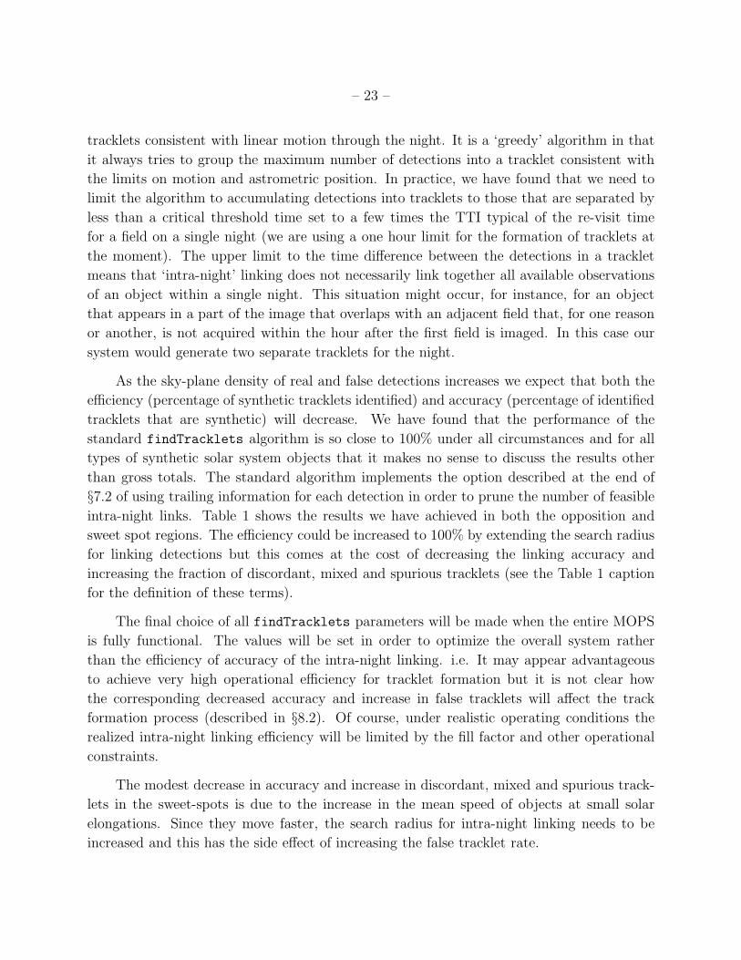
– 23 –

tracklets consistent with linear motion through the night. It is a ‘greedy’ algorithm in that

it always tries to group the maximum number of detections into a tracklet consistent with

the limits on motion and astrometric position. In practice, we have found that we need to

limit the algorithm to accumulating detections into tracklets to those that are separated by

less than a critical threshold time set to a few times the TTI typical of the re-visit time

for a field on a single night (we are using a one hour limit for the formation of tracklets at

the moment). The upper limit to the time difference between the detections in a tracklet

means that ‘intra-night’ linking does not necessarily link together all available observations

of an object within a single night. This situation might occur, for instance, for an object

that appears in a part of the image that overlaps with an adjacent field that, for one reason

or another, is not acquired within the hour after the first field is imaged. In this case our

system would generate two separate tracklets for the night.

As the sky-plane density of real and false detections increases we expect that both the

efficiency (percentage of synthetic tracklets identified) and accuracy (percentage of identified

tracklets that are synthetic) will decrease. We have found that the performance of the

standard findTracklets algorithm is so close to 100% under all circumstances and for all

types of synthetic solar system objects that it makes no sense to discuss the results other

than gross totals. The standard algorithm implements the option described at the end of

§7.2 of using trailing information for each detection in order to prune the number of feasible

intra-night links. Table 1 shows the results we have achieved in both the opposition and

sweet spot regions. The efficiency could be increased to 100% by extending the search radius

for linking detections but this comes at the cost of decreasing the linking accuracy and

increasing the fraction of discordant, mixed and spurious tracklets (see the Table 1 caption

for the definition of these terms).

The final choice of all findTracklets parameters will be made when the entire MOPS

is fully functional. The values will be set in order to optimize the overall system rather

than the efficiency of accuracy of the intra-night linking. i.e. It may appear advantageous

to achieve very high operational efficiency for tracklet formation but it is not clear how

the corresponding decreased accuracy and increase in false tracklets will affect the track

formation process (described in §8.2). Of course, under realistic operating conditions the

realized intra-night linking efficiency will be limited by the fill factor and other operational

constraints.

The modest decrease in accuracy and increase in discordant, mixed and spurious track-

lets in the sweet-spots is due to the increase in the mean speed of objects at small solar

elongations. Since they move faster, the search radius for intra-night linking needs to be

increased and this has the side effect of increasing the false tracklet rate.

– 24 –

Note that the total number of tracklets available in a lunation is in excess of 1.3 million

corresponding to almost 450,000 different objects. Thus, in a single lunation Pan-STARRS

may identify and obtain orbits and colors for more solar system objects than are currently

known. The PS1 proto-type system with only a single telescope will not perform as well but

will still identify on the order of as many objects as are currently known in a single lunation.

Table 2 shows the effect of not using each detection’s trailing information when per-

forming findTracklets (see §7.2 for a brief discussion of the use of trailing information

when creating tracklets). As expected, the efficiency can remain high only at the expense of

realizing one-third the accuracy and nearly an order of magnitude more false tracklets.

8.2. Track Identification

The algorithm for inter-night linking of tracklets is called linkTracklets. Once a night

of detections has been processed by findTracklets (§8.1) blocks of (usually contiguous)

images in the same region of sky are grouped together for processing by linkTracklets in a

‘pass’ (see table 3). A database query identifies all other tracklets obtained in the surrounding

area (increasing sky-plane distance with time) within the last 14 days and if there are three

available nights for linking within that time frame then linkTracklets attempts to link

those tracklets together.

The number of images that may be grouped together depends on the density of tracklets

and the length of time over which inter-night linking is attempted. In general, we find that

beyond the 14 day limit the linking algorithm becomes inefficient and inaccurate. Traversing

a large gap in time to look for linkages is prohibitive because there are too many potential

linkages that satisfy the requirement of quadratic motion and too many real objects are

non-quadratic over the same time period and will not be identified. We limit the range

of acceptable speeds from 0.0◦/day to 10.0◦/day where the lower limit allows us to detect

extremely slow moving distant objects and the upper limit is set by our funding agency. The

maximum acceleration was set to 0.02◦/day2 in both RA and declination.

Note that the term ‘inter-night’ linking is strictly not correct due to the time limit on

the spacing of intra-night tracklets as described in §8.1. Inter-night linking actually links

together all tracklets between and within nights when available.

Table 3 gives various performance statistics for the linkTracklets algorithm. To test

the performance as a function of the sky-plane density of objects we generated four different

models as described in the table caption. The realized sky-plane density of synthetic objects

in the field varies over two orders of magnitude while the tracks that were available for

– 25 –

linking ranged over more than three orders. In each case the false detections were kept at

the expected density of 250 deg−2 for Pan-STARRS operations.

Inter-night linking efficiency decreases slowly with the realized sky-plane density of

synthetic tracks as shown in table 3. Even at densities expected for the full four telescope

Pan-STARRS system with a limiting magnitude of r ∼ 24mag the track creation efficiency

is currently above 98%.

Of more concern is the effect of sky-plane density on the accuracy of track creation -

the fraction of synthetic tracks compared to all identified tracks. When there are no false

detections the accuracy of track creation is nearly 100% because even with a full density

solar system model (for Pan-STARRS-4) the sky-plane density of tracklets is low enough to

make confusion unimportant. Since the next step in the MOPS after track creation is to

attempt an initial orbit determination (IOD) on each identified track, the accuracy needs to

be high in order to not waste too many CPU cycles on attempting orbits on tracks that are

not valid. However, calculating an IOD for tracks is trivially parallelizable.

Note that the accuracy increases in table 3 in the first three steps of increasing asteroid

sky-plane density but drops precipitously on the last jump. This is due to the fact that we

used a constant false detection rate equal to the expected density of false detections in all

four simulations. Thus, in the first three runs the noise is dominated by the false detections

but in the last run the density of synthetic detections becomes high enough to add extra

confusion into the linking process.

At this point we have not put much effort into increasing the accuracy of the linkTracklets

algorithm but there are many opportunities to do so. One such possibility is a multiple pass

scenario in which we first attempt to link the ‘easy’ tracklets (i.e. everything from the Main

Belt outwards) with relatively tight constraints on their night-to-night motion, remove the

tracklets that survive orbit determination in good tracks, and then loosen the constraints in

order to identify difficult objects (NEOs). We tested this technique on a simulation involving

over 22,000 tracklets in over 352,000 tracks. Removing the properly linked tracklets, and all

false tracks containing any of those tracklets, left only about 6,700 tracks. Thus, this could

be a powerful technique for increasing the effectiveness of the inter-night linking process.

The decrease in accuracy of linkTracklets at full density is accompanied by a dramatic

increase in the run time. Increasing the sky-plane density by a factor of about six increases

the runtime by a factor of almost thirty. This is also not of particular concern because

the linking algorithm is easily parallelizable. The parallelization of linkTracklets is easily

implemented by running each ‘pass’ (described above) on a different processor. The sky-

plane density of tracklets becomes high enough in the final simulation of table 3 to require

– 26 –

tripling the number of passes.

Tables 4 through 7 show the progression of linking efficiency as a function of both the

sky-plane density and the solar system object type. The efficiency is high for all classes

of objects and for all densities as would be expected after table 3. There is a very slight

decrease in linking efficiency for each object class as their sky-plane density increases. Within

each model (each table) there is a slight increase in linking efficiency with increasing mean

heliocentric distance of the object class.

The high efficiency for NEOs and distant objects should not be surprising. While

their sky-plane density is low compared to the MB objects, their rates of motion are often

anomalous. Even though the distant objects do not move very far in a transient time interval

and therefore provide little motion vector information, the sky-plane density of slow moving

objects is low enough to make the linking efficiency very high.

In §5 it was pointed out that the survey pattern avoids the ’stationary spots’ and thus

it must be remembered that the results quoted herein do not provide results for all-sky

inter-night linking efficiency. The intra-night linking efficiency should be much better in the

stationary spots because the detections will be much closer together than at other points

along the objects orbits. However, it is reasonable to expect that the inter-night linking

efficiency will decrease in the stationary spots due to the unusual apparent acceleration of

the objects in this region.

As mentioned earlier in this section, the MOPS has restricted its requirements to linking

only those objects with tracklets on three nights within a lunation. The more difficult

problem of linking and confirming just two nights of tracklets in one lunation or linking

three tracklets across two lunations is not handled with the algorithms described here. To

extend the discovery phase space into this realm we have teamed with Andrea Milani who

will provide us software capable of making these links. The theoretical framework for his

work has been described elsewhere (Milani et al. 2005) and the realized efficiencies in Pan-

STARRS simulations will be discussed in a future paper.

8.3. MOPS and other surveys

Contemporary wide-field asteroid surveys only perform the intra-night linking step.

They identify asteroids by their linear motion in a single night on three or more images.

The intra-night linking efficiency has been measured by some of the major NEO surveys by

attempting to identify known asteroids in their fields. The measured peak efficiency for aster-

oids well above the limiting magnitude varies from about 65% (Spacewatch; Jedicke & Herron

– 27 –

(1997)), ∼ 70% (Catalina Sky Survey, observatory 703; Beshore personal communication),

∼ 90% (Catalina Sky Survey, observatory G96; Beshore personal communication), and about

90% for the latest and reprocessed Spacewatch data (Larsen et al. 2001). In both these sur-

vey’s the intra-night linkings proposed by their algorithms are checked by a human observer.

This is clearly an impossible task at the Pan-STARRS discovery rate.

Some of the targeted (pencil-beam or narrow field) surveys have determined their intra-

night detection efficiency by injecting synthetic asteroid images directly into the images

before running their source detection and linking algorithms (e.g. Gladman et al. 2006;

Petit et al. 2004). They realize efficiencies of ∼90%.

Inter-night linking is mostly performed by the Minor Planet Center and there has been

no report on their efficiency for this process.

To test the MOPS on real data before the onset of Pan-STARRS we have obtained

raw source detection lists from the Spacewatch (Larsen et al. 2001; Jedicke & Herron 1997)

asteroid survey. We have passed their data through the MOPS and have identified apparently

realistic asteroids. In order to reduce the number of clearly false orbits identified by MOPS we

needed to run two pre-filters on the set of detections they provide. The first eliminates regions

on the sky with unusual over-densities of detections. The over-densities are a problem in the

Spacewatch automated reduction process due to mis-estimating the background level. The

second pre-filter reduces the prevalence of anomalous sets of detections in linear features. The

Spacewatch source finding algorithm identifies many false detections in the linear features

associated with bright star diffraction spikes, CCD edge effects and artifical satellite streaks.

Figure 14 shows the distribution of ‘derived’ objects - those objects for which MOPS

formed tracklets, tracks, initial orbit determination and differentially corrected orbits. Since

the figure shows final orbital elements for the derived objects it goes beyond the purview of

merely intra and inter-night linking as discussed in the rest of this work. This is done for

two reasons: 1) because most of the Spacewatch detections are previously unknown objects

it would be difficult for us to establish which tracklets and tracks were false and real and 2)

to show that the MOPS is operational on real data. The system efficiency through initial

and differential orbit determination will be described in a future paper.

9. Conclusion

The Pan-STARRS project has developed the first integrated asteroid detection, intra

and inter-night linking, attribution, precovery, orbit identification and orbit determination

system in the world. It is known as the Moving Object Processing System (MOPS). For test-

– 28 –

ing and monitoring purposes during operations we have developed a peudo-realistic simula-

tion of the system including a realistic survey strategy incorporating simple weather factors,

S/N-dependent astrometric noise and false detections at a sky-plane density expected for the

four telescope Pan-STARRS system. The simulation does not include additional important

factors such as the camera fill factor or probabilistic detections near the detection threshold.

We have developed new algorithms based on kd-tree and variable-trees to link detections

within and between nights that dramatically improve the speed of identification and that

scale as O(ρ log ρ) where ρ is the sky-plane density of objects. The implementation of the

algorithms is trivially parallelizable on a set of CPU nodes.

Using these algorithms we have demonstrated nearly 100% efficiency for intra-night

linking of synthetic detections with realistic properties into ‘tracklets’. Furthermore, we

have demonstrated the ability to obtain nearly 100% efficiency for linking those tracklets

over many nights into ‘tracks’. The accuracy of the algorithm, the fraction of identified

tracks that are actually synthetic in the presence of noise, depends on and decreases with

the sky-plane density of detections.

Tests of the MOPS intra and inter-night linking algorithms on real data provided by the

Spacewatch facility show that the system is capable of handling real data with all its inherent

systematic problems that are otherwise not explored in our synthetic surveying model.

– 29 –

Acknowledgements

The design and construction of the Panoramic Survey Telescope and Rapid Response

System by the University of Hawaii Institute for Astronomy is funded by the United States

Air Force Research Laboratory (AFRL, Albuquerque, NM) through grant number F29601-

02-1-0268. The MOPS is currently being developed in association with the Large Synoptic

Survey Telescope (LSST). Jeremy Kubica’s work was funded in part by the LSST and by a

grant from the Fannie and John Hertz Foundation. The LSST’s research and development

effort is funded in part by the National Science Foundation under Scientific Program Order

No. 9 (AST-0551161) through Cooperative Agreement AST-0132798. Additional funding

comes from private donations, in-kind support at Department of Energy laboratories and

other LSSTC Institutional Members. Spacewatch (Robert McMillan) provided source de-

tections for testing the MOPS procedures. Paulo Holvorcem provided timely assistance for

creating synthetic surveys.

– 30 –

REFERENCES

Bar-Shalom, Y., and Li, X-R. 1995. Multitarget-Multisensor Tracking: Principles and Tech-

niques. Published by Yaakov Bar-Shalom, Storrs, CT.

Bar-Shalom, Y., Li, X-R, and Kirubarajan, T. 2001. Estimation with Applications to

Tracking and Navigation: Theory Algorithms and Software. Published by Wiley-

Interscience, New York, NY.

Bentley, J. L. 1975. Multidimensional Binary Search Trees Used for Associative Searching.

Communications of the ACM, 18, 9, 509-517.

Bernstein, G. M., Trilling, D. E., Allen, R. L., Brown, M. E., Holman, M., Malhotra, R.

2004. The Size Distribution of Trans-Neptunian Bodies.AJ128, 1364-1390.

Blackman, S. and Popoli, R. 1999. Design and Analysis of Modern Tracking Systems. Pub-

lished by Artech House, Boston, MA.

Boattini, A. and 11 co-authors. 2006. The Campo Imperatore Near Earth Object Survey

(CINEOS). Submitted to ‘Earth, Moon and Planets’.

Bottke, W. F., Morbidelli, A., Jedicke, R., Petit, J.-M., Levison, H. F., Michel, P., and

Metcalfe, T. S. 2002. Debiased Orbital and Absolute Magnitude Distribution of the

Near-Earth Objects. Icarus 156, 399-433.

E. Bowell, K. Muinonen, and L. H. Wasserman. 1994. A public-domain asteroid orbit

database. In ”Asteroids, Comets, Meteors 1993” (A. Milani et al., eds.), pp. 477-

481. Kluwer, Dordrecht

Bowell, E. and Muinonen, K. 1994. Earth-crossing Asteroids and Comets: Groundbased

Search Strategies. Hazards Due to Comets and Asteroids, p. 149.

Bowell, E., Hapke, B., Domingue, D., Lumme, K., Peltoniemi, J., Harris, A. W. 1989.

Application of photometric models to asteroids. Asteroids II 524-556.

Chesley, S. R. and Spahr, T. B. 2004. Earth impactors: orbital characteristics and warning

times. Mitigation of Hazardous Comets and Asteroids, 22.

Denneau, L., . 2006. The Pan-STARRS Solar System Model. In preparation.

Denneau, L. 2006. The Pan-STARRS Solar System Survey Simulation. In preparation.

– 31 –

Elliot, J. L., and 10 colleagues 2005. The Deep Ecliptic Survey: A Search for Kuiper Belt

Objects and Centaurs. II. Dynamical Classification, the Kuiper Belt Plane, and the

Core Population.AJ129, 1117-1162.

Gladman, B. J. and 11 co-authors. 2006. A sub-kilometer asteroid diameter survey. Submit-

ted to Icarus.

Granvik, M. and Muinonen, K. 2005. Asteroid identification atdiscovery. Icarus 179, 109-127.

Gauss, K. F. 1809. Hambvrgi, Svmtibvs F. Perthes et I. H. Besser, 1809.

Harris, A. W. 1998. Evaluation of ground-based optical surveys for near-Earth asteroids.

Planet. Space Sci.46, 283-290.

Hodapp, K. W., and 30 colleagues 2004. Design of the Pan-STARRS telescopes. Astronomis-

che Nachrichten 325, 636-642.

Jedicke, R., Morbidelli, A., Spahr, T., Petit, J.-M., and Bottke, W. F. 2003. Earth and

space-based NEO survey simulations: prospects for achieving the spaceguard goal.

Icarus 161, 17-33.

Jedicke, R., Larsen, J., and Spahr, T. 2002. Observational Selection Effects in Asteroid

Surveys. Asteroids III, 71-87.

Jedicke, R. and Herron, J. D. 1997. Observational Constraints on the Centaur Population.

Icarus 127, 494-507.

Jedicke, R. 1996. Detection of Near Earth Asteroids Based Upon Their Rates of Motion.

AJ111, 970.

Jewitt, D. C., Trujillo, C. A., Luu, J. X. 2000. Population and Size Distribution of Small

Jovian Trojan Asteroids.AJ120, 1140-1147.

Kaiser, N. 2004. . The Likelihood of Point Sources in Pixellated Images. Pan-STARRS in-

ternal document PSDC-200-010-00 available upon request.

Kristensen, L. K. 2004. Initial Orbit Determination for Distant Objects. AJ127, 2424-2435.

Kristensen, L. K. 2002. Follow-up Ephemerides and the Accuracy of Preliminary Orbits.

Icarus 159, 339-350.

Kristensen, L. K. 1992. The identification problem in asteroid surveys. A&A262, 606-612.

– 32 –

Kubica, J., Moore, A., Connolly, R., and Jedicke, R. 2005. A Multiple Tree Algorithm for the

Efficient Association of Asteroid Observations. The Eleventh ACM SIGKDD Interna-

tional Conference on Knowledge Discovery and Data Mining (2005), ACM Press, Eds.

Robert L. Grossman and Roberto Bayardo and Kristin Bennett and Jaideep Vaidya,

p. 138-146.

Kubica, J., Masiero, J., Moore, A., Jedicke, R., and Connolly, R. 2005. Variable kd-Tree

Algorithms for Spatial Pattern Search and Discovery. Advances in Neural Information

Processing Systems, MIT Press, Eds. Y. Weiss and B. Scholkopf and J. Platt, p. 691-

698.

Larsen, J. A., Gleason, A. E., Danzl, N. M., Descour, A. S., McMillan, R. S., Gehrels, T.,

Jedicke, R., Montani, J. L., Scotti, J. V. 2001. The Spacewatch Wide-Area Survey for

Bright Centaurs and Trans-Neptunian Objects. Astronomical Journal 121, 562-579.

Masiero, J. et al. 2006. The CFHT Main Belt G-survey. in preparation.

Marsden, B. G. 1985. Initial orbit determination - The pragmatist’s point of view. AJ90,

1541-1547.

McKee, C. F. with Taylor, T. F. and 13 co-authors. 2001. Astronomy and Astrophysics in the

New Millennium. Library of Congress Card Number: 00-112257, National Academy

Press, Washington, DC.

Mignard, F. 2002. Observations of solar system objects with GAIA. I. Detection of NEOS.

A&A393, 727-731.

Milani, A., Gronchi, G. F., Knezevic, Z., Sansaturio, M. E., Arratia, O., Denneau, L., Grav,

T., Heasley, J., Jedicke, R., Kubica, J. 2006. Unbiased orbit determination for the

next generation asteroid/comet surveys. IAU Symposium 229, 367-380.

Milani, A., Gronchi, G. F., Knezevic, Z., Sansaturio, M. E., and Arratia, O. 2005. Orbit

determination with very short arcs. Icarus 179, 350-374.

Milani, A., Sansaturio, M. E., and Chesley, S. R. 2001. The Asteroid Identification Problem

IV: Attributions. Icarus 151, 150-159.

Milani, A., La Spina, A., Sansaturio, M. E., and Chesley, S. R. 2000. The Asteroid Identifi-

cation Problem. III. Proposing Identifications. Icarus 144, 39-53.

Milani, A. and Valsecchi, G. B. 1999. The Asteroid Identification Problem. II. Target Plane

Confidence Boundaries. Icarus 140, 408-423.

– 33 –

Milani, A. 1999. The Asteroid Identification Problem. I. Recovery of Lost Asteroids. Icarus

137, 269-292.

Morrison, D. 1992. The Spaceguard Survey - Protecting the earth from cosmic impacts.

Mercury 21, 103-106.

Petit, J.-M., Holman, M., Scholl, H., Kavelaars, J., Gladman, B. 2004. A highly automated

moving object detection package. MNRAS347, 471-480.

Raymond, S. N., and 23 colleagues 2004. A Strategy for Finding Near-Earth Objects with

the SDSS Telescope. AJ127, 2978-2987.

Stokes, G. H., Evans, J. B., and Larson, S. M. 2002. Near-Earth Asteroid Search Programs.

Asteroids III, 45-54.

Tedesco, E. F., Cellino, A., and Zappala, V. 2005. The Statistical Asteroid Model. I. The

Main-Belt Population for Diameters Greater than 1 Kilometer. AJ129, 2869-2886.

Tonry, J., Burke, B. E., Schechter, P. L. 1997. The Orthogonal Transfer CCD. PASP109,

1154-1164.

Yoshida, F., Nakamura, T., Watanabe, J.-I., Kinoshita, D., Yamamoto, N., Fuse, T. 2003.

Size and Spatial Distributionsof Sub-km Main-Belt Asteroids. PASJ55, 701-715.

Virtanen, J., Muinonen, K., and Bowell, E. 2001. Statistical Ranging of Asteroid Orbits.

Icarus 154, 412-431.

This preprint was prepared with the AAS LATEX macros v5.2.

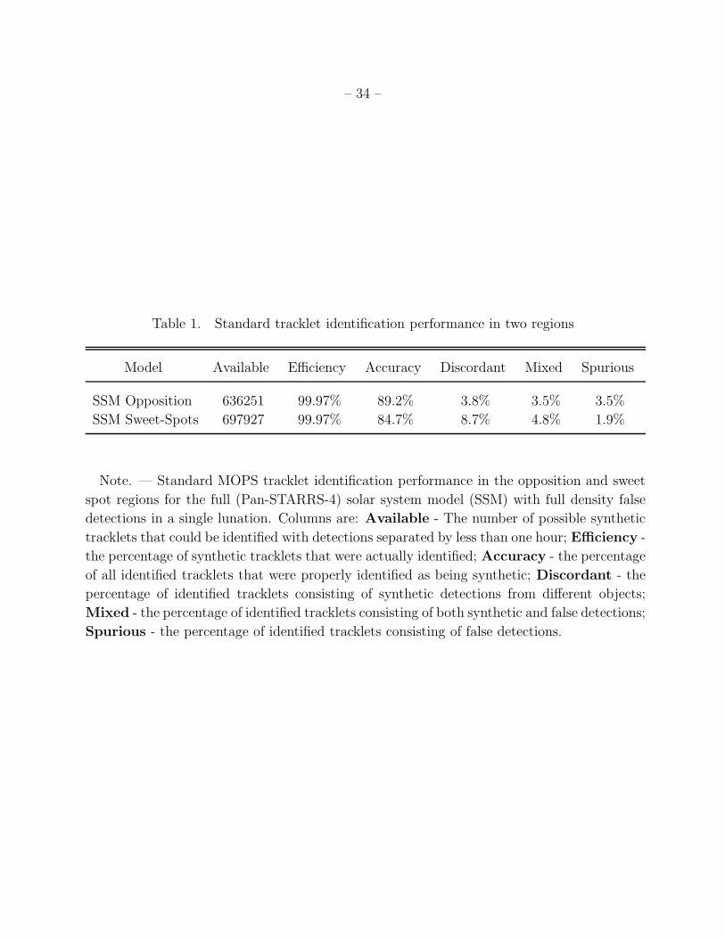
– 34 –

Table 1. Standard tracklet identification performance in two regions

Model Available Efficiency Accuracy Discordant Mixed Spurious

SSM Opposition 636251 99.97% 89.2% 3.8% 3.5% 3.5%

SSM Sweet-Spots 697927 99.97% 84.7% 8.7% 4.8% 1.9%

Note. — Standard MOPS tracklet identification performance in the opposition and sweet

spot regions for the full (Pan-STARRS-4) solar system model (SSM) with full density false

detections in a single lunation. Columns are: Available - The number of possible synthetic

tracklets that could be identified with detections separated by less than one hour; Efficiency -

the percentage of synthetic tracklets that were actually identified; Accuracy - the percentage

of all identified tracklets that were properly identified as being synthetic; Discordant - the

percentage of identified tracklets consisting of synthetic detections from different objects;

Mixed - the percentage of identified tracklets consisting of both synthetic and false detections;

Spurious - the percentage of identified tracklets consisting of false detections.

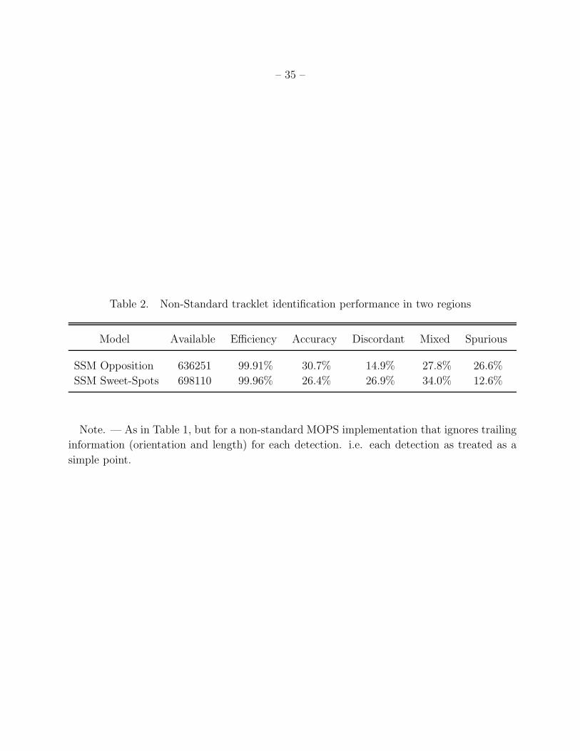
– 35 –

Table 2. Non-Standard tracklet identification performance in two regions

Model Available Efficiency Accuracy Discordant Mixed Spurious

SSM Opposition 636251 99.91% 30.7% 14.9% 27.8% 26.6%

SSM Sweet-Spots 698110 99.96% 26.4% 26.9% 34.0% 12.6%

Note. — As in Table 1, but for a non-standard MOPS implementation that ignores trailing

information (orientation and length) for each detection. i.e. each detection as treated as a

simple point.

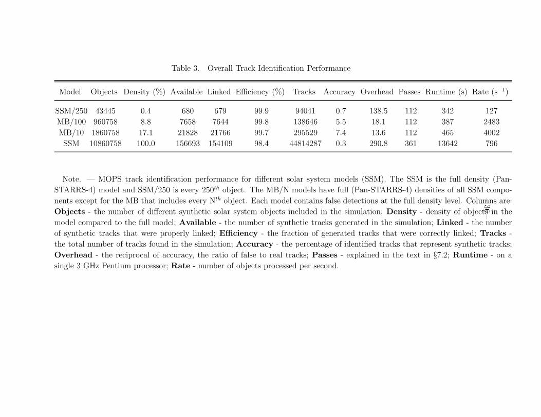
–36

–

Table 3. Overall Track Identification Performance

Model Objects Density (%) Available Linked Efficiency (%) Tracks Accuracy Overhead Passes Runtime (s) Rate (s−1)

SSM/250 43445 0.4 680 679 99.9 94041 0.7 138.5 112 342 127

MB/100 960758 8.8 7658 7644 99.8 138646 5.5 18.1 112 387 2483

MB/10 1860758 17.1 21828 21766 99.7 295529 7.4 13.6 112 465 4002

SSM 10860758 100.0 156693 154109 98.4 44814287 0.3 290.8 361 13642 796

Note. — MOPS track identification performance for different solar system models (SSM). The SSM is the full density (Pan-

STARRS-4) model and SSM/250 is every 250th object. The MB/N models have full (Pan-STARRS-4) densities of all SSM compo-

nents except for the MB that includes every Nth object. Each model contains false detections at the full density level. Columns are:

Objects - the number of different synthetic solar system objects included in the simulation; Density - density of objects in the

model compared to the full model; Available - the number of synthetic tracks generated in the simulation; Linked - the number

of synthetic tracks that were properly linked; Efficiency - the fraction of generated tracks that were correctly linked; Tracks -

the total number of tracks found in the simulation; Accuracy - the percentage of identified tracks that represent synthetic tracks;

Overhead - the reciprocal of accuracy, the ratio of false to real tracks; Passes - explained in the text in §7.2; Runtime - on a

single 3 GHz Pentium processor; Rate - number of objects processed per second.

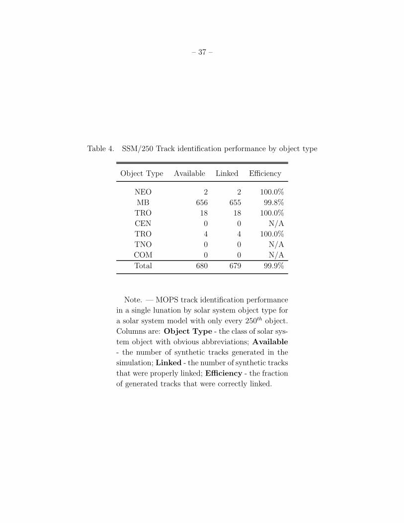
– 37 –

Table 4. SSM/250 Track identification performance by object type

Object Type Available Linked Efficiency

NEO 2 2 100.0%

MB 656 655 99.8%

TRO 18 18 100.0%

CEN 0 0 N/A

TRO 4 4 100.0%

TNO 0 0 N/A

COM 0 0 N/A

Total 680 679 99.9%

Note. — MOPS track identification performance

in a single lunation by solar system object type for

a solar system model with only every 250th object.

Columns are: Object Type - the class of solar sys-

tem object with obvious abbreviations; Available

- the number of synthetic tracks generated in the

simulation; Linked - the number of synthetic tracks

that were properly linked; Efficiency - the fraction

of generated tracks that were correctly linked.

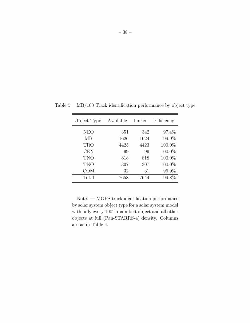
– 38 –

Table 5. MB/100 Track identification performance by object type

Object Type Available Linked Efficiency

NEO 351 342 97.4%

MB 1626 1624 99.9%

TRO 4425 4423 100.0%

CEN 99 99 100.0%

TNO 818 818 100.0%

TNO 307 307 100.0%

COM 32 31 96.9%

Total 7658 7644 99.8%

Note. — MOPS track identification performance

by solar system object type for a solar system model

with only every 100th main belt object and all other

objects at full (Pan-STARRS-4) density. Columns

are as in Table 4.

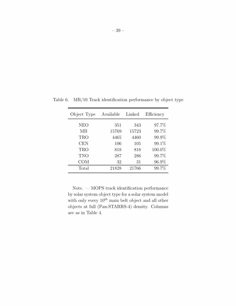
– 39 –

Table 6. MB/10 Track identification performance by object type

Object Type Available Linked Efficiency

NEO 351 343 97.7%

MB 15769 15723 99.7%

TRO 4465 4460 99.9%

CEN 106 105 99.1%

TRO 818 818 100.0%

TNO 287 286 99.7%

COM 32 31 96.9%

Total 21828 21766 99.7%

Note. — MOPS track identification performance

by solar system object type for a solar system model

with only every 10th main belt object and all other

objects at full (Pan-STARRS-4) density. Columns

are as in Table 4.

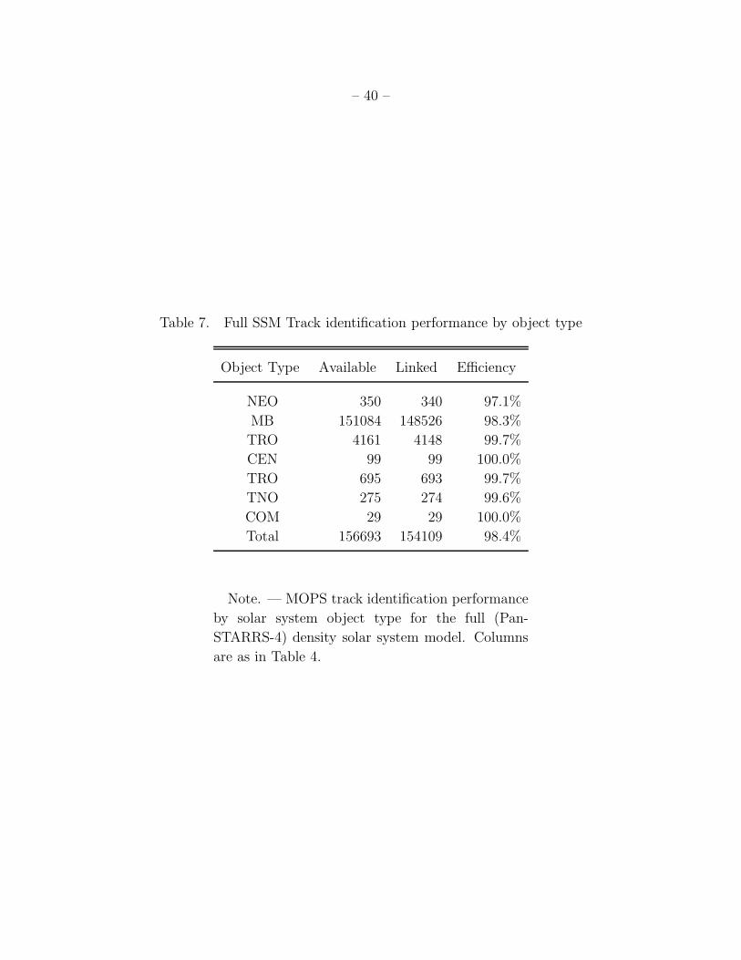
– 40 –

Table 7. Full SSM Track identification performance by object type

Object Type Available Linked Efficiency

NEO 350 340 97.1%

MB 151084 148526 98.3%

TRO 4161 4148 99.7%

CEN 99 99 100.0%

TRO 695 693 99.7%

TNO 275 274 99.6%

COM 29 29 100.0%

Total 156693 154109 98.4%

Note. — MOPS track identification performance

by solar system object type for the full (Pan-

STARRS-4) density solar system model. Columns

are as in Table 4.

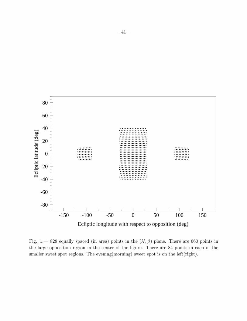
– 41 –

-80

-60

-40

-20

0

20

40

60

80

-150 -100 -50 0 50 100 150

Ecliptic longitude with respect to opposition (deg)

Ecl

iptic

latit

ude

(deg

)

Fig. 1.— 828 equally spaced (in area) points in the (λ′, β) plane. There are 660 points in

the large opposition region in the center of the figure. There are 84 points in each of the

smaller sweet spot regions. The evening(morning) sweet spot is on the left(right).

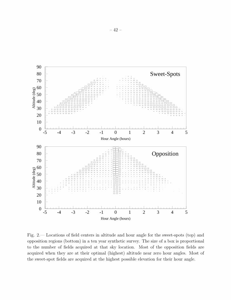
– 42 –

0

10

20

30

40

50

60

70

80

90

-5 -4 -3 -2 -1 0 1 2 3 4 5Hour Angle (hours)

Alti

tude

(de

g)

Sweet-Spots

0

10

20

30

40

50

60

70

80

90

-5 -4 -3 -2 -1 0 1 2 3 4 5Hour Angle (hours)

Alti

tude

(de

g)

Opposition

Fig. 2.— Locations of field centers in altitude and hour angle for the sweet-spots (top) and

opposition regions (bottom) in a ten year synthetic survey. The size of a box is proportional

to the number of fields acquired at that sky location. Most of the opposition fields are

acquired when they are at their optimal (highest) altitude near zero hour angles. Most of

the sweet-spot fields are acquired at the highest possible elevation for their hour angle.

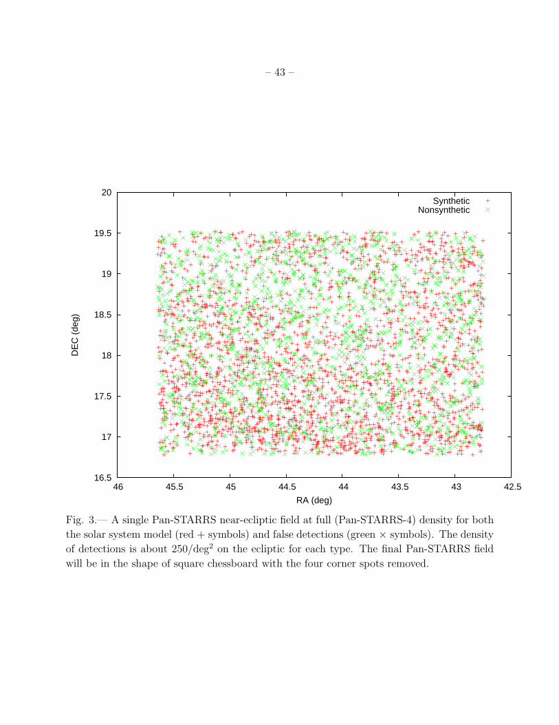
– 43 –

16.5

17

17.5

18

18.5

19

19.5

20

42.5 43 43.5 44 44.5 45 45.5 46

DE

C (

deg)

RA (deg)

SyntheticNonsynthetic

Fig. 3.— A single Pan-STARRS near-ecliptic field at full (Pan-STARRS-4) density for both

the solar system model (red + symbols) and false detections (green × symbols). The density

of detections is about 250/deg2 on the ecliptic for each type. The final Pan-STARRS field

will be in the shape of square chessboard with the four corner spots removed.

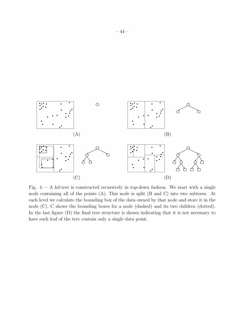
– 44 –

(A) (B)

(C) (D)

Fig. 4.— A kd-tree is constructed recursively in top-down fashion. We start with a single

node containing all of the points (A). This node is split (B and C) into two subtrees. At

each level we calculate the bounding box of the data owned by that node and store it in the

node (C). C shows the bounding boxes for a node (dashed) and its two children (dotted).

In the last figure (D) the final tree structure is shown indicating that it is not necessary to

have each leaf of the tree contain only a single data point.

– 45 –

Recursive kd-Tree Range Search

Input: Current Tree Node T, query point q, radius r.

Output: A list of matching points Z

1. IF q is within r node T’s bounding box:

2. IF T is a leaf node:

3. FOR each data point x owned by node T:

4. IF q is within r of x:

5. Add x to Z.

6. ELSE

7. Recursively search using each T’s children nodes in place of T.

8. Return Z

Fig. 5.— A recursive search for points within radius r of the query point q using a kd-tree.

This search is initially called with the root node of the kd-tree.

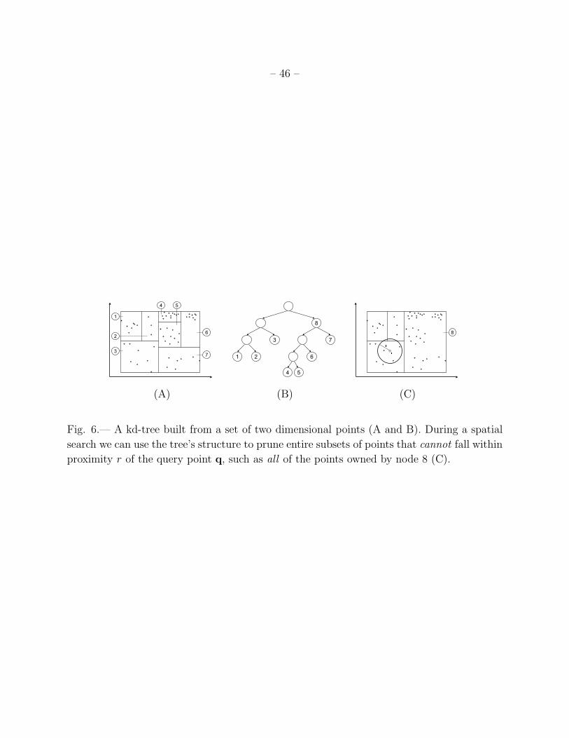
– 46 –

(A) (B) (C)

Fig. 6.— A kd-tree built from a set of two dimensional points (A and B). During a spatial

search we can use the tree’s structure to prune entire subsets of points that cannot fall within

proximity r of the query point q, such as all of the points owned by node 8 (C).

– 47 –

Sequential Intra-Night Linkage Algorithm

Input: A set X of all input detections

Output: A list of result tracks Z

1. Build a kd-Tree on the detections X.

2. FOR each tracklet x ∈ X:

3. Use the kd-tree to efficiently find Y the set of all reachable detections.

4. FOR each potential pairing (x ∈ X,y ∈ Y):

5. Create a new linear tracklet z from x and y.

6. Use the kd-tree (or the set Y) to find all supporting detections

compatible with z.

7. IF z has enough support.

8. Add z to Z.

9. Return Z

Fig. 7.— A simplified multiple hypothesis tracking algorithm for asteroid linkage.

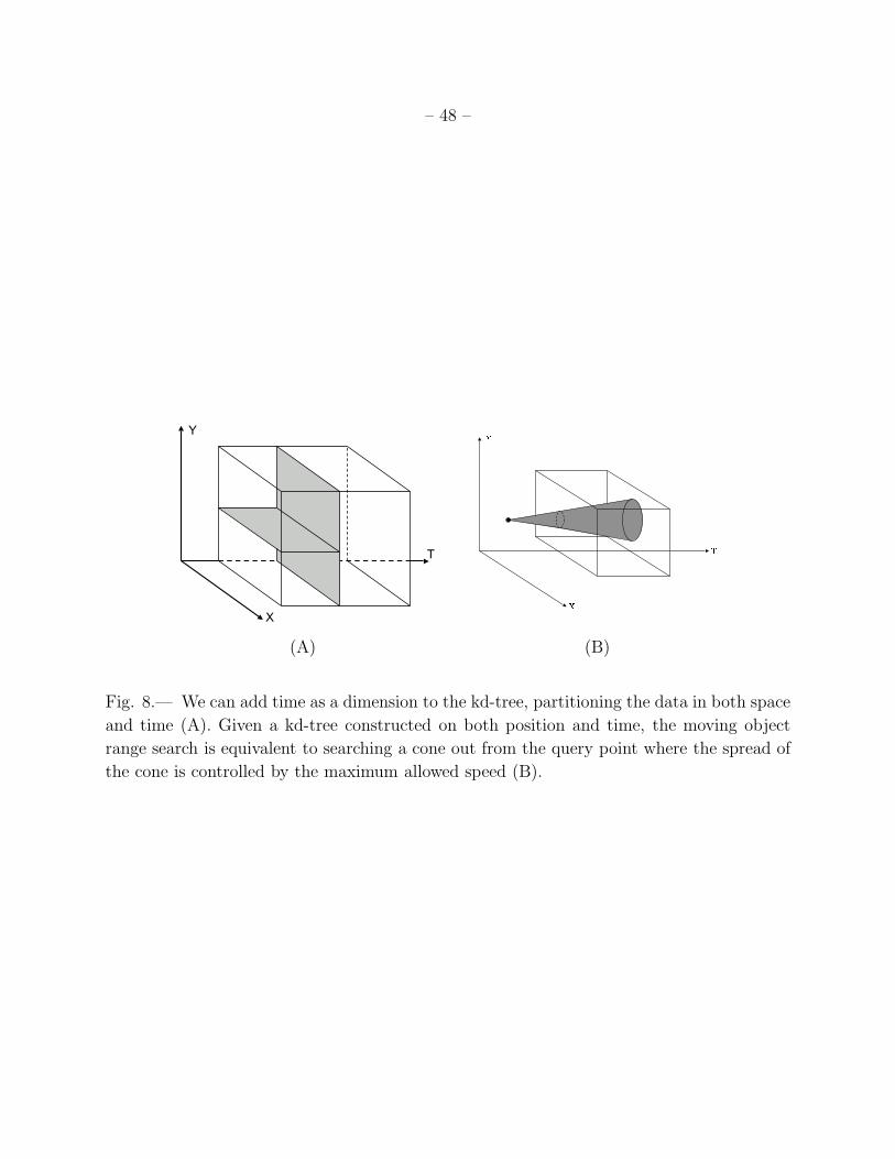
– 48 –

(A) (B)

Fig. 8.— We can add time as a dimension to the kd-tree, partitioning the data in both space

and time (A). Given a kd-tree constructed on both position and time, the moving object

range search is equivalent to searching a cone out from the query point where the spread of

the cone is controlled by the maximum allowed speed (B).

– 49 –

Moving Object Range Search

Input: A query point q, a current tree node T, and

minimum and maximum speeds: vmin and vmax.

Output: A list of feasible points Z

1. If we cannot prune T as per Equations 4 and 5:

2. IF T is a leaf node:

3. FOR each x owned by T:

4. v = dist(q,x)|tq−tx|

5. IF vmin ≤ v ≤ vmax:

6. Add x to Z.

7. ELSE:

8. Recursively search using T’s left child.

9. Recursively search using T’s right child.

10. Return Z.

Fig. 9.— The recursive algorithm for a moving object range search.

– 50 –

Fig. 10.— The model nodes’ bounds (1 and 2) define a region of feasible support (shaded)

for any combination of model points from those nodes.

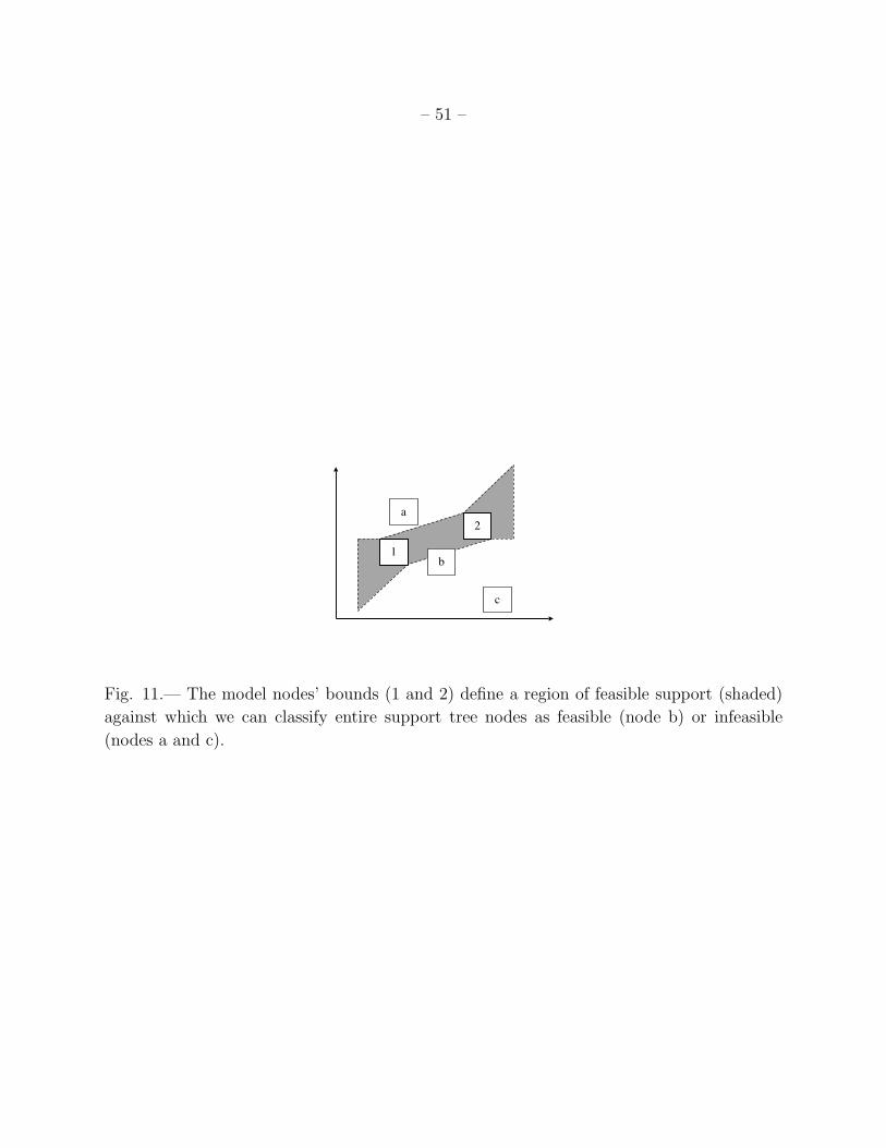
– 51 –

Fig. 11.— The model nodes’ bounds (1 and 2) define a region of feasible support (shaded)

against which we can classify entire support tree nodes as feasible (node b) or infeasible

(nodes a and c).

– 52 –

Variable-Tree Model Detection

Input: A set of M current model tree nodes M

A set of current support tree nodes S

Output: A list Z of feasible sets of points

1. S′ ← {} and Scurr ← S

2. IF we cannot prune based on the mutual compatibility of M:

3. FOR each s ∈ Scurr

4. IF s is compatible with M:

5. IF s is “too wide”:

6. Add s’s left and right child to the end of Scurr.

7. ELSE

8. Add s to S′.

9. IF we have enough valid support points:

10. IF all of m ∈M are leaves:

11. Test all combinations of points owned by the model nodes, using

the support nodes’ points as potential support.

Add valid sets to Z.

12. ELSE

13. Let m∗ be the non-leaf model tree node that owns the most points.

14. Search using m∗’s left child in place of m∗ and S′ instead of S.

15. Search using m∗’s right child in place of m∗ and S′ instead of S.

Fig. 12.— A simple variable-tree algorithm for spatial structure search. This algorithm uses

simple heuristics such as: searching the model node with the most points and splitting a

support node if it is too wide. These heuristics can be replaced by more accurate, problem-

specific ones.

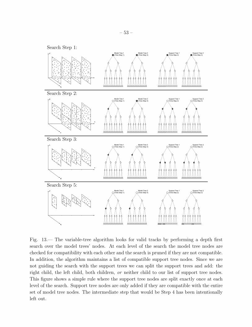
– 53 –

Search Step 1:

Search Step 2:

Search Step 3:

Search Step 5:

Fig. 13.— The variable-tree algorithm looks for valid tracks by performing a depth first

search over the model trees’ nodes. At each level of the search the model tree nodes are

checked for compatibility with each other and the search is pruned if they are not compatible.

In addition, the algorithm maintains a list of compatible support tree nodes. Since we are

not guiding the search with the support trees we can split the support trees and add: the

right child, the left child, both children, or neither child to our list of support tree nodes.

This figure shows a simple rule where the support tree nodes are split exactly once at each

level of the search. Support tree nodes are only added if they are compatible with the entire

set of model tree nodes. The intermediate step that would be Step 4 has been intentionally

left out.

– 54 –

0

0.2

0.4

0.6

0.8 1

0 2

4 6

8 1

0

Eccentricity (e)

Sem

i-Maj

or A

xis

(a),

AU

Sem

i-Maj

or A

xis

(a)

vs. E

ccen

tric

ity (

e), 1

346

Orb

its

q=1.

3 A

U N S0

Fig. 14.— Eccentricity versus semi-major axis for objects identified in raw Spacewatch de-

tections i.e. in their entire transient source detection list, not just the list of observations

reported to the MPC. The crosses represent presumably real objects identified in their as-

trometry while the x’s represent synthetic NEOs emplaced in the data and subsequently

identified by MOPS. Note that one of the synthetic NEOs is identified with a non-NEO

orbit.