arX

iv:a

stro

-ph/

9706

219v

1 2

0 Ju

n 19

97Mon. Not. R. Astron. Soc. 000, 000–000 (0000) Printed 1 February 2008 (MN LATEX style file v1.4)

Probing the Universe with the Lyman-alpha Forest:

I. Hydrodynamics of the Low Density IGM

Nickolay Y. Gnedin1 and Lam Hui21Department of Astronomy, University of California, Berkeley, CA 947202NASA/Fermilab Astrophysics Center, Fermi National Accelerator Laboratory, Batavia, IL 60510

1 February 2008

ABSTRACT

We introduce an efficient and accurate alternative to full hydrodynamic simula-tions, Hydro-PM (HPM), for the study of the low column density Lyman-alpha forest(NHI

<∼

1014 cm−2). It consists of a Particle-Mesh (PM) solver, modified to compute,in addition to the gravitational potential, an effective potential due to the gas pres-sure. Such an effective potential can be computed from the density field because of atight correlation between density and pressure in the low density limit (δ <

∼10), which

can be calculated for any photo-reionization history by a method outlined in Hui &Gnedin (1997). Such a correlation exists, in part, because of minimal shock-heating inthe low density limit. We compare carefully the density and velocity fields as well asabsorption spectra, computed using HPM versus hydrodynamic simulations, and findgood agreement. We show that HPM is capable of reproducing measurable quantities,such as the column density distribution, computed from full hydrodynamic simula-tions, to a precision comparable to that of observations. We discuss how, by virtueof its speed and accuracy, HPM can enable us to use the Lyman-alpha forest as acosmological probe.

We also discuss in detail the smoothing of the gas (or baryon) fluctuation relativeto that of the dark matter on small scales due to finite gas pressure: (1) It is shownthe conventional wisdom that the linear gas fluctuation is smoothed on the Jeans scaleis incorrect for general reionization (or reheating) history; the correct linear filteringscale is in general smaller than the Jeans scale after reheating, but larger prior toit. (2) It is demonstrated further that in the mildly nonlinear regime, a PM solver,combined with suitable pre-filtering of the initial conditions, can be used to model thelow density IGM. But such an approximation is shown to be less accurate than HPM,unless a non-uniform pre-filtering scheme is implemented.

Key words: cosmology: theory — intergalactic medium — quasars: absorption lines– methods: numerical – hydrodynamics

1 INTRODUCTION

The low density intergalactic medium, filling the enormousspace between galaxies and their aggregations, offers cos-mologists a unique and powerful probe of the high redshiftuniverse (z ∼ 2 − 5), still inaccessible for large galaxy sur-veys. The intergalactic medium (hereafter IGM) manifestsitself observationally in the numerous weak absorption linesalong a line of sight to a distant quasar, the Lyman-alphaforest. Up to date, an enormous treasury of observationaldata on the Lyman-alpha forest at a wide range of redshiftshas been collected (see, for example, Hu et al. 1995, Lu et al.1996, Cristiani et al. 1996, Kirkman & Tytler 1997, Kim etal. 1997 and D’Odorico et al. 1997 for most recent observa-

tional advances). Several models were proposed to explainthe Lyman-alpha forest (Bahcall & Salpeter 1965; Arons1972; Black 1981; Ostriker & Ikeuchi 1983; Ikeuchi & Os-triker 1986; Rees 1986; Ikeuchi 1986; Rees 1988; Bond, Sza-lay, & Silk 1988; McGill 1990; Bi, Borner & Chu 1992). How-ever, it was only after several groups (Cen et al. 1994; Zhang,Anninos, & Norman 1995; Hernquist et al. 1996; Miralda-Escude et al. 1996; Wadsley & Bond 1996; Zhang et al. 1997)performed cosmological hydrodynamic simulations when itbecame apparent that at least an appreciable fraction of theLyman-alpha forest consists of smooth fluctuations in theIGM, which arise naturally under gravitational instability,rather than discrete absorbers, as has been believed before.

Abundance of observational data and the existence of

c© 0000 RAS

2 Gnedin and Hui

a compelling theoretical framework (i.e. hierarchical clus-tering) allows one to make detailed comparisons betweenobservations and predictions of a given cosmological model.Moreover, one might even attempt to use the observationaldata in a maximum-likehood type analysis to infer cosmo-logical parameters, either in a model-independent way, or atleast within a class of models. A recent example towards thisdirection is the use of the observed mean Lyman-alpha opti-cal depth to put limits on the baryon content of the universe(Miralda-Escude et al. 1996; Rauch, et al.1996; Bi & David-sen 1997; Weinberg et al. 1997). One might contemplategoing a step further to use other properties of the Lyman-alpha forest as a probe of equally interesting cosmologicalparameters such as the normalization and slope of the powerspectrum (see, for example, Hui, Gnedin & Zhang 1997), themassive neutrino density, the epoch of reionization and soon.

However, while hydrodynamic simulations give us in-sights into the physical properties of the IGM as well as def-inite predictions for a given cosmological model (provided,numerical resolution and physical modelling are adequate),computational expense makes them impractical to use in amaximum-likehood type of analysis in which a large rangeof models are considered.

It is therefore important to ask whether a more effi-cient, and at the same time sufficiently accurate, approxi-mate method can be developed in place of full hydrodynamicsimulations.

Up to date, two different semi-analytical approxi-mations have been used: the lognormal approximation(Bi, Borner & Chu 1992; Bi & Davidsen 1997; Gnedin& Hui 1996) and the (truncated) Zel’dovich approxima-tion (Doroshkevich, & Shandarin 1977; McGill 1990; Hui,Gnedin, & Zhang 1997). While both approximations are veryefficient, they might not be sufficiently accurate. For exam-ple, while the one-point density distribution function is closeto lognormal for mildly nonlinear fluctuations, the lognormalapproximation itself fails to reproduce the density field ac-curately (Coles, Melott, & Shandarin 1993). The truncatedZel’dovich approximation is somewhat more accurate, andcan be used for about a decade in the IGM density, fromabout ρ/3 to 3ρ, where ρ is the average density of the uni-verse. However, a main drawback of the truncated Zel’dovichapproximation is the necessity of the smoothing of the ini-tial density field to minimize the amount of orbit-crossingby the time of interest. This inevitably introduces artificialsmoothing of small scale structure, which could bias one’spredictions, depending on the quantities one is interested in.While the Zel’dovich approximation can be successfully ap-plied to study the column density distribution of the Lyman-alpha forest (Hui, Gnedin, & Zhang 1997), it remains to beseen whether it can reproduce the detailed results of a hy-drodynamic simulation with sufficient accuracy.

In this paper we present a new approximate method,which is based on a standard Particle-Mesh (PM) solver,modified to account for the pressure forces acting on a fluidelement. While the PM solver is significantly slower than,say, the Zel’dovich approximation, it is still much fasterthan a full hydrodynamic simulation. In order to developa method that will be accurate to within 15% (the reasonfor this number will be clear by §4), we first in §2 describetwo hydrodynamic simulations that we have run to be used

as templates against which approximate methods are com-pared. Then, we start with linear theory to develop someintuition first. In §3 we discuss the effect of the gas pres-sure on the evolution of linear perturbations. The conven-tional wisdom that linear baryon (or gas) perturbations aresmoothed on the Jeans scale is shown to be incorrect ingeneral, and it is demonstrated that the smoothing scaledepends on the reionization history of the universe. Armedwith an understanding of the behavior of linear fluctuations,in §4 we compare full hydrodynamic simulations with anapproximate method based on combining a PM solver withthe appropriate smoothing of initial conditions (with thesmoothing scale motivated by the linear analysis), as a wayof taking into account the physical effect of gas pressure(this is different from initial smoothing in the case of thetruncated Zel’dovich approximation as a way of correctingfor orbit-crossing). We then conclude that this method isnot sufficiently accurate and proceed to develop our newapproximation, which we call Hydro-PM (hereafter HPM)in §5.

The idea of HPM is very simple: one modifies a regularPM solver to compute, in addition to the usual gravitationalpotential, an effective potential due to the presence of gaspressure. This is possible because there exists a tight cor-relation between temperature and density (or equivalently,between pressure and density) in the low density limit, whichcan be computed quite accurately for any given reionizationhistory (Hui & Gnedin 1997). A given density field thenpredicts an effective pressure field as well as a definite grav-itational potential field. The fundamental rationale is thatfor the Lyman-alpha forest of sufficiently low column den-sity (NHI <∼ 1014 cm−2), shock-heating is not important (or,equivalently, the density fluctuations are only mildly non-linear, δ <∼ 10), which is the one piece of physics that HPMdoes not incorporate. As we will show, this does not com-promise our accuracy significantly while buying us a greatincrease in efficiency over full hydrodynamic simulations.

It is appropriate that we mention here two wonderfulpieces of related work. Petitjean, Mucket & Kates (1995) andMucket et al. (1996) investigated properties of the Lyman-alpha forest using PM simulations, suitably modified to fol-low the thermodynamics of baryons. Their approach differfrom our HPM method in at least two aspects: the baryonsare approximated as following trajectories of dark matterprior to shell-crossing (we include the dynamical effects ofpressure on baryons), and shock-heating is modelled in theirmethod which enables them to study higher column densitysystems. The reader is referred to the above papers for de-tails.

Finally, we conclude in §6 with a brief discussion. Aword on our notation: the symbol ρ is used to denote massdensity as usual, as well as the mass density in units of thecosmic mean (i.e. ρ and 1 + δ used interchangeably). Whichmeaning is intended should be clear from the context.

2 HYDRODYNAMIC SIMULATIONS

We have performed two cosmological hydrodynamic sim-ulations against which we will measure the performanceof our approximate methods. We used the SLH-P3M codeas described by Gnedin (1995), Gnedin (1996), Gnedin &

c© 0000 RAS, MNRAS 000, 000–000

Hydrodynamics of the IGM 3

Table 1. Cosmological Models

Model Ω0 Ωb h ΩΛ σ8 cell size

LCDM 0.35 0.055 0.7 0.65 0.79 6.6h−1 kpcSCDM 1.0 0.05 0.5 0 0.70 15.6h−1 kpc

Figure 1. Evolution of the ionizing intensity J21 for the LCDMmodel (solid line) and the SCDM model (dashed line) as a func-tion of redshift.

Bertschinger (1996) and Gnedin & Ostriker (1997). Table2 contains cosmological parameters of the two models. Wehave chosen two different models which enable us to test ourapproximate methods under different conditions. For bothmodels we have used 643 baryonic mesh and the softeningparameter was set to 1/3, which gives us a dynamical rangeof 192. Since we are mainly concerned with modelling thelow density IGM, δ <∼ 10, we do not need to set the softeningparameter to a very small value. Our choice of the softeningparameter, however, does enable full resolution of regionswith δ = 10 or lower. The LCDM model is identical to themodel used in our Equation of State paper (Hui & Gnedin1997), except for the larger value of the softening parame-ter, while the SCDM model is close to the model studied byZhang et al. (1997).

The thermal history for each of our simulations is de-termined by the evolution of the photo-ionizing background.Figure 1 shows the evolution of the ionizing intensity J21 asa function of redshift for both hydrodynamic simulations.The redshift evolution of J21 and the spectrum of radiationfor the LCDM model was adopted from the simulation de-scribed in (Hui & Gnedin 1997). For the SCDM model, wehave adopted the following form of the redshift evolution ofJ21:

J21(z) =1

2

[

1 + tanh

(

1007 − z

8(1 + z)

)]

,

where J21 is defined in exactly the same way as JHI in Hui& Gnedin (1997), and we adopt the same spectral shapeas in Hui & Gnedin (1997), equation (7). This form of theredshift evolution of J21 is close to the sudden reioniza-tion models discussed in detail in Hui & Gnedin (1997). Forlow z, z ≪ 7, the ionizing intensity reaches its asymptoticvalue, J21 = 1.0, and it drops quickly before the redshift ofreionization, zrei = 7. The factor of 100 inside the tanh in-

sures that reionization occurs smoothly in a redshift interval∆z/z ∼ 0.01. This transition period is introduced to avoidnumerical instabilities possible when J21 increases abruptlyat the redshift of reionization, as in models of sudden reion-ization.

Both simulations have been continued until z = 3.It is worth pointing out that the simulation box in bothcases was rather small, 1h−1 Mpc for the LCDM model, and422h−1 kpc for the SCDM model. At the final redshift, fluc-tuations at the box size are already nonlinear, and simu-lation boxes are not representative patches of the universe.This fact should have minimal effect on the present work: ourmain goal is to develop an understanding of the relationshipbetween the dark matter and the baryons on small scales, tohelp us find an approximation that takes into account bothgravity and gas pressure in an appropriate manner (on largescales, things are simple: dark matter and baryons simplytrace each other). The key is then to resolve structure onthe relevant small (mass) scales (as will be explained in thenext section), rather than having a representative sample ofthe universe on large scales.

3 LINEAR EVOLUTION OF COSMOLOGICAL

PERTURBATIONS

The linear evolution of perturbations in the dark matter- baryon fluid is governed by two second order differentialequations:

d2δX

dt2+ 2H

dδX

dt= 4πGρ(fXδX + fbδb),

d2δb

dt2+ 2H

dδb

dt= 4πGρ(fXδX + fbδb) −

c2Sa2k2δb, (1)

where δX(t, k) and δb(t, k) are Fourier components of den-sity fluctuations in the dark matter and baryons (we equatebaryons with the cosmic gas in this paper) respectively,which have respective mass fractions fX and fB , H(t) is theHubble constant, a(t) is the cosmological scale factor, ρ(t) isthe average mass density of the universe, cS(t) is the soundspeed in the cosmic gas (where the sound speed is simplydefined by c2S ≡ dP/dρ, assuming an equation of state thatrelates the P and ρ), k is the comoving wavenumber and tis the proper time.

In the limit where the dark matter is gravitationallydominant, fb = 0 in equation (1), the growth of δX is de-scribed by the familiar factor D+(t) (Peebles 1980), whichcoincides with a(t) if the matter density of the universe iscritical.

The right hand side of the equation for δb contains twoterms: the gravitational force and the pressure force. Onlarge scales, in the limit k → 0, the pressure force can beneglected, and the baryon fluctuation obeys the same equa-tion as the dark matter fluctuation. Assuming that δb = δX

initially, we have

δb(t, k → 0) = δX(t, k → 0) ∝ D+(t).

On small scales, k → ∞, the pressure force is dominant,and one would expect that the baryon fluctuation is sup-pressed compared to the dark matter fluctuation. A charac-teristic scale, where the two forces are equal, is called the

c© 0000 RAS, MNRAS 000, 000–000

4 Gnedin and Hui

Jeans scale. We denote the wavenumber corresponding tothe Jeans scale as kJ ,

kJ =a

cS

√

4πGρ. (2)

The Jeans scale is in general a function of time, but for thespecial case when the gas temperature T evolves with timeas T ∝ 1/a, the Jeans scale is constant in time. In this case,and assuming fb = 0 (i.e. the baryons are gravitationallysubdominant), so that δX ∝ D+, equation (1) can be solvedanalytically:

δb(t, k) =δX(t, k)

1 + k2/k2J

. (3)

Thus, at small scales, k → ∞, the baryon fluctuation issuppressed relative to the dark matter fluctuation by a factorof k2

J/k2. Note that this assumes effectively a very special

boundary condition: T ∝ 1/a at all times.Let us now consider a more realistic case. At sufficiently

high redshifts, before the Compton heating of the baryongas by the CMB becomes inefficient, the evolution of thebaryon temperature is well described by the T ∝ 1/a law.At redshifts of about 100 (depending on the baryon densityof the universe), Compton scattering becomes inefficient andthe temperature of the baryon gas drops adiabatically, T ∝1/a2. By low redshifts, but before the universe reionizes,the gas temperature can be treated as effectively zero (orin other words, the Jeans mass associated with the CMBtemperature is too small to be relevant for the modelling ofthe Lyman-alpha forest).

The gas temperature rises dramatically after the uni-verse reionizes, and its subsequent evolution is obviously ourobject of interest. As we will show, equations (2) and (3) nolonger provide a correct description of the smoothing andtime evolution of the gas.

In order to consider a realistic case, we extract the evo-lution of the sound speed from our SCDM simulation andsolve equation (1) numerically with the obtained form ofcs(t).

Figure 2 shows the linear baryon fluctuation, normal-ized by the linear dark matter fluctuation, at z = 3. Threedifferent cases are shown: fb = 0.05 as in the simulation (thesolid line), fb = 0 in equation (1), baryons being treatedas gravitationally subdominant and therefore their gravita-tional effect is negligible (the dashed line), and fb = 1, allmatter being baryonic (the dotted line). The two cases withfb = 0.05 and fb = 0 can barely be distinguished from eachother in the figure. The case where all the matter is treatedas baryonic also gives a very similar result. This point willbe examined further in §6.

Let us focus on the open circles for the time being. Theyrepresent the linear baryon fluctuation as given by equation(3), where the filtering scale is the Jeans scale as definedin equation (2) for z = 3. One can see that in this realisticcase (where T does not evolve as 1/a at all times), filteringof the baryon fluctuation occurs at a smaller scale than theJeans scale, contrary to conventional wisdom. In addition,oscillations occur at small scales, and the amplitude of theseoscillations decay at a rate slower that 1/k2, contrary toequation (3).

It is possible to understand this analytically. Let us con-sider the case where the baryons are gravitationally sub-dominant, fb = 0. Then the dark matter fluctuation simply

Figure 2. Comparisons of different filtering. The exact linearbaryon fluctuation for the SCDM model at z = 3 as calculatedfrom equation (1) are shown for fb = 0.05 (solid line), fb = 0(dashed line, almost overlapping with the solid line), and fb = 1(dotted line). Points with different symbols represent differentfiltering of the linear dark matter fluctuation (to approximatethe linear baryon fluctuation): 1/(1 + k2/k2

J ) filtering (open cir-cles), exp(−k2/k2

F ) filtering (filled circles), 1/(1+k2/k2F ) filtering

(filled triangles), and a hybrid filtering which gives the best fit tothe envelope of the baryon fluctuation (eq. [20]; stars).

grows like D+(t) (ignoring the decaying mode). Let us con-sider expanding the ratio of the baryon fluctuation to darkmatter fluctuation δb(t, k)/δX(t, k) in powers of k2. Retain-ing only the first two dominant terms in the small k limit,and recalling that δb(t, k = 0) = δX(t, k = 0), we have:

δb(t, k)

δX(t, k)= 1 −

A(t)

D+(t)k2, (4)

where A(t) is an unknown coefficient to be determined. In-serting equation (4) into (1) and ignoring terms of order k4

or higher, we obtain the following equation for A(t):

d2A

dt2+ 2H

dA

dt=c2Sa2D+(t). (5)

This equation can be easily solved by:

A(t) =

∫ t

0

dt′c2S(t′)D+(t′)

∫ t

t′

dt′′

a2(t′′). (6)

where the initial conditions A(t = 0) = dA/dt(t = 0) = 0are assumed (i.e. no difference between the baryon and darkmatter fluctuations at early times). Note that A is pos-itive, which means the baryon fluctuation is always sup-pressed, compared to the dark matter, in the low k regime.We now introduce the filtering scale, with the correspondingwavenumber denoted as kF , by the following expression:

A(t) ≡D+(t)

k2F (t)

,

so that equation (4) can now be rewritten as

c© 0000 RAS, MNRAS 000, 000–000

Hydrodynamics of the IGM 5

δb(t, k)

δX(t, k)= 1 −

k2

k2F

. (7)

The following expression for the filtering scale kF can beobtained:

1

k2F (t)

=1

D+(t)

∫ t

0

dt′a2(t′)D+(t′) + 2H(t′)D+(t′)

k2J (t′)

∫ t

t′

dt′′

a2(t′′), (8)

where we have replaced the sound speed by its expression interms of the Jeans scale at the same moment (eq. [2]), anddot denotes differentiation with respect to the time t.

An important conclusion follows from equation (8). Letus rewrite it in the following form, using the median valuetheorem:

1

k2F (t)

=1

k2J (t∗)

[

1

D+(t)

∫ t

0

dt′a2(t′)

(

D+(t′) + 2H(t′)D+(t′))

∫ t

t′

dt′′

a2(t′′)

]

,

where t∗ is between 0 and t. The expression in square brack-ets integrates to 1, and we obtain:

kF (t) = kJ(t∗), (9)

where t∗ ≤ t. In other words, the filtering scale at a giventime is equal to the Jeans scale at some earlier time. Inparticular, if the Jeans scale 1/kJ is an increasing function oftime, which is typically the case for sufficiently low redshiftsafter reionization, the filtering scale 1/kF is always smaller

than the Jeans scale. The reverse would be true prior toreionization, as we will see in a moment.

The above notion of the filtering scale is, strictly speak-ing, only applicable in the small k limit, because it is de-rived based on an expansion in k2 (equation [4]). To see howwell this filtering scale provides a description of the linearbaryon fluctuation in the high k regime, we show in Fig. 2with filled circles the filtering in the form exp(−k2/k2

F ) (i.e.δb = δX exp[−k2/k2

F ]), where kF is computed from equation(8) using the evolution of the sound speed (or in other wordsthe Jeans scale) as extracted from the SCDM hydrodynamicsimulation.

One can see despite the fact that kF is derived in thesmall k limit, the exponential filtering with kF gives an ex-cellent fit to the baryon fluctuation even for high k, untiloscillations take over. We also show with filled triangles thefiltering of the form 1/(1+k2/k2

F ) (i.e. δb = δX/[1+k2/k2F ])

for the same kF , which gives a worse fit for the high k cut-offand, as in the case of exp(−k2/k2

F ) filtering, does not matchthe envelope of oscillations on small scales.

Encouraged by the excellent performance of the gaus-sian filtering on scale of 1/kF in reproducing the exact lin-ear solution, we now consider a few special cases, where kF

can be calculated analytically. Let us restrict ourselves toan Ω0 = 1 universe, where D+(t) = a(t). For simplicity,we will assume that the mean molecular weight of the cos-mic gas does not change, in which case the sound speed isdirectly proportional to the square root of the gas tempera-ture. First, we consider the case where the gas temperatureT is zero before reionization (which occurs at a = arei), andremains constant thereafter:

T =

0, a < arei, andT0, otherwise.

(10)

Computing the integral (8), we obtain for a > arei:

1

k2F

=1

k2J

3

10

[

1 + 4(

arei

a

)5/2

− 5(

arei

a

)2]

. (11)

In particular, for a≫ arei,

kF =

√

10

3kJ .

Another instructive example is when the gas tempera-ture decays as 1/a after reionization,

T =

0, a < arei, andT0arei/a, otherwise.

(12)

In this case the filtering scale for a > arei is given by

1

k2F

=1

k2J

[

1 + 2(

arei

a

)3/2

− 3arei

a

]

. (13)

In the limit a≫ arei we recover the standard result kF = kJ ,but the asymptote is reached only slowly, and even at z = 3and for zrei = 7, we obtain kF = 2.2kJ . We emphasize thedeparture of the correct filtering scale from the usual Jeansscale is a result of the fact that T above is not assumedto evolve as 1/a at all times. The time evolution of T con-sidered above is partly motivated by reionization models inwhich the originally cool cosmic gas was heated up to a hightemperature by radiation emitted by sources (stars, quasars,etc) that turned on at some high redshift.

Typically, the gas temperature decays as an interme-diate power between a0 and a−1 after reionization (Hui &Gnedin 1997). We, therefore, conclude that in a realistic caseone should expect that at z ∼ 3 the filtering scale of the cos-mic gas is about a factor of 1.5− 2.5 smaller than the Jeansscale, unless the universe reionized at a very high redshift,zrei ≫ 10.

Another interesting example is the evolution of thebaryon perturbations before reionization. After recombina-tion at z ∼ 1200, the cosmic gas temperature is still cou-pled to the CBR temperature by Compton heating, andtherefore evolves as T ∝ 1/a. At a later time adec =0.01(Ωbh

2/0.0125)2/5 , Compton heating becomes inefficient,and the gas temperature decreases adiabatically, T ∝ 1/a2.Since the Jeans scale decreases with time for an adiabaticallycooling gas, the filtering scale for the cosmic gas is actuallylarger than the Jeans scale. More precisely, a good approx-imation to the evolution of the cosmic gas temperature isgiven by the following expression:

T =

2.73 K/a, a < adec, and2.73 Kadec/a

2 otherwise.(14)

In this case the filtering scale for a > adec is given by

1

k2F

=1

k2J

[

3 ln(a/adec) − 3 + 4(

adec

a

)1/2]

. (15)

For example, for Ωbh2 = 0.0125, kF = 0.45kJ at z = 10, and

in term of masses, the characteristic mass scale on which thegas distribution is smoothed, MF ∝ 1/k3

F , is about 11 timeslarger than the Jeans scale, MJ ∝ 1/k3

J . This result hasimportant implications for understanding the formation ofthe first bound objects in the universe.

c© 0000 RAS, MNRAS 000, 000–000

6 Gnedin and Hui

Next, we turn our attention to the oscillations in thehigh k regime, a behavior we can understand analyticallyfor the time evolution specified in equation (12). We cansolve equation (1) exactly in this case, assuming once againthe case of an Ω0 = 1 universe with fb = 0 (i.e. baryonsbeing gravitationally subdominant):

δb(t, k)

δX(t, k)=

1

1 + k2/k2J

(

1 +k2

k2J

[

n−

n− − n+

(

a

arei

)n+

−

n+

n− − n+

(

a

arei

)n−

])

(16)

for a > arei, where

n± = −5

4±

3

4

√

1

9−

8

3

k2

k2J

,

and where δX grows as a. Note that since T ∝ 1/a at a >arei, the Jeans scale kJ is constant in time. In the limita ≫ arei and for k sufficiently small, equation (16) reducesto equation (3).

Let us now consider a fixed final a, and take the largek limit. Then both n+ and n− become complex (but δb isstill real), and δb as a function of k oscillates. However, onecan see that in the high k limit, the amplitude of these os-cillations is independent of k. We, therefore, conclude thatin general δb/δX has no power-law asymptote in the high klimit. It is sometimes claimed in the literature that δb/δX

always approaches an asymptote of k−2 in the high k limit.That statement is only correct if T evolves as a fixed powerlaw in a at all times (see Bi et al. 1992 for derivation). Thesimple case above provides an example of departure fromthis property.

Finally, we emphasize that the two hydrodynamic sim-ulations described in the previous section have sufficientlysmall cell sizes so that the corresponding correct filteringscales (1/kF ) are resolved by about 5 mesh cells. This en-sures that we can meaningfully compare different smoothingprescriptions, as explained in the following section.

4 FILTERING INITIAL CONDITIONS FOR A

PM SIMULATION

The linear analysis in the previous section shows that thetwo mass components, the dark matter and the cosmic gas,evolve differently on small scales: the dark matter is affectedby gas pressure only via gravitational interaction with thegas, while the gas evolution is directly influenced by the ther-mal pressure on sufficiently small scales. In order to computethis complex interaction in every detail, a two-componenthydrodynamic simulation is needed. But often the preci-sion achieved by the full hydrodynamic simulation is notrequired. For instance, current observations of the Lyman-alpha forest typically give about 10-15% accuracy for thecolumn density distribution. We will attempt to develop anapproximation, that is significantly faster than a hydrody-namic simulation, but at the same time gives us results withsimilar accuracy.

As a step toward this goal, we will concentrate in thispaper on single-component approximations, i.e. approxima-tions where the evolution of the cosmic gas is computed

using only one set of resolution elements (in our case parti-cles) instead of following both the dark matter and the gasseparately. This approach is certainly more economical thana full hydrodynamic simulation, but the question is: can wemake it accurate enough?

It is certainly possible to emulate a gas-dynamic solverusing a simple dark matter solver in the linear regime. Letδ(0)X (t, k) and δ

(0)b (t, k) be the linear solutions to equation (1)

for a specific cosmological model. Suppose we are interestedin the baryon fluctuation at some final moment t = tf (whichis early enough so that the fluctuation remains linear). Let usmodel the evolution of the baryon perturbation with a dark-matter-only solver (e.g. PM), which, in the linear regime, isequivalent to solving the first of equations (1) and assumingfb = 0. If we choose the following initial condition for thedark-matter-only solver at an early time t = ti:

δX(t = ti, k) =D+(ti)

D+(tf )δ(0)b (t = tf , k), (17)

it is easy to see that we will reproduce the baryon fluctuationin the linear regime at t = tf . Since, as we have shown in the

last section, δ(0)b (t = tf , k) can be modelled by δX(t = tf , k)

multiplied by some suitable filter, the above initial conditionis equivalent to smoothing the initial δX with the same filter.

One might then hope to model the dynamical evolutionof the gas by a PM simulation, with the initial conditions ap-propriately smoothed. In other words, one may try to modelthe gas evolution under the assumption that the gas is in-fluenced by gravity alone, hoping that the initial filteringprocedure is sufficient to model the effect of pressure.

There is no guarantee that this simple-minded methodwould work. After all, our idea of a simple filtering scale isderived from linear analysis, while for our applications, weare interested in regions of space with overdensity below,but reaching up to about 10. In fact, we will show in thissection that this method works to a certain extent, but is not

good enough, i.e. it fails to achieve an accuracy of 10− 15%in a point-by-point comparison of density and velocity fieldsagainst full hydrodynamic simulations. Observationally, in-teresting quantities such as the column density distributionare typically measured with an accuracy of about 10− 15%.As we will show in the next section, this level of accuracyrequires similar accuracies in the density and velocity fieldsthemselves.

Before we embark upon a quantitative comparison ofthe PM + filtering method versus hydrodynamic simulation,we have to address one technical point.

A collisionless (alias “N-body”) numerical simulation,such as PM, uses particles to follow the evolution of thesystem. For our applications, it is eventually necessary tocompute the gas density and velocity as a function of spa-tial positions. How does one convert a distribution of par-ticles into, say, the density field? There exist several tech-niques, but in this paper we will adopt the simplest methodof assigning the density onto a uniform mesh using parti-cle weights. Specifically, we will use the Triangular-Shape-Clouds (TSC) scheme to assign the particle density onto amesh. This method, however, suffers from numerical noise.For example, in a sufficiently underdense region a particlemight be so remote from its neighbors that the TSC assign-ment would leave empty regions (zero density) between theparticle and some of its neighbors. This generates unphys-

c© 0000 RAS, MNRAS 000, 000–000

Hydrodynamics of the IGM 7

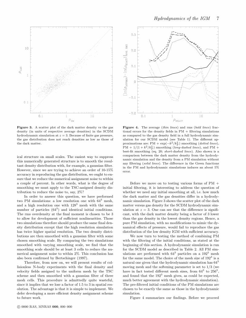
Figure 3. A scatter plot of the dark matter density vs the gasdensity (in units of respective average densities) in the SCDMhydrodynamic simulation at z = 3. Because of finite gas pressure,the gas distribution does not reach densities as low as those ofthe dark matter.

ical structure on small scales. The easiest way to suppressthis numerically generated structure is to smooth the resul-tant density distribution with, for example, a gaussian filter.However, since we are trying to achieve an order of 10-15%accuracy in reproducing the gas distribution, we ought to en-sure that we reduce the numerical assignment noise to withina couple of percent. In other words, what is the degree ofsmoothing we must apply to the TSC-assigned density dis-tribution to reduce the noise to, say, 2%?

In order to answer this question, we have performedtwo PM simulations: a low resolution one with 643 mesh,and a high resolution one with 1283 mesh with the samenumber of particles (643) and identical initial conditions.The rms overdensity at the final moment is chosen to be 3to allow for development of sufficient nonlinearities. Thosetwo simulations therefore should produce the same final den-sity distribution except that the high resolution simulationhas twice higher spatial resolution. The two density distri-butions are then smoothed with a gaussian filter with somechosen smoothing scale. By comparing the two simulationssmoothed with varying smoothing scale, we find that thesmoothing scale should be at least 3 cells to reduce the nu-merical assignment noise to within 2%. This conclusion hasalso been confirmed by Bertschinger (1997).

Therefore, from now on, we will present results of col-lisionless N-body experiments with the final density andvelocity fields assigned to the uniform mesh by the TSCscheme and then smoothed with a gaussian filter of threemesh cells. This procedure is admittedly quite wasteful,since it implies that we lose a factor of 1.5 to 3 in spatial res-olution. The advantage is that it is simple to implement. Wedefer developing a more efficient density assignment schemeto future work.

Figure 4. The average (thin lines) and rms (bold lines) frac-tional errors for the density fields in PM + filtering simulationsas compared to the gas density field in a full hydrodynamic sim-ulation for our SCDM model (see Table 1). The different ap-proximations are: PM + exp(−k2/k2

F ) smoothing (dotted lines),PM + 1/(1 + k2/k2

F ) smoothing (long-dashed lines), and PM +best-fit smoothing (eq. 20; short-dashed lines). Also shown is acomparison between the dark matter density from the hydrody-namic simulation and the density from a PM simulation withoutany filtering (solid lines). The difference in the Green functionsin the PM and hydrodynamic simulations induces an about 5%error.

Before we move on to testing various forms of PM +initial filtering, it is interesting to address the question ofwhether we need any initial smoothing at all, i.e. how muchthe dark matter and the gas densities differ in a hydrody-namic simulation. Figure 3 shows the scatter plot of the darkmatter versus gas density for the SCDM hydrodynamic sim-ulation at z = 3. One can see that the difference is signifi-cant, with the dark matter density being a factor of 3 lowerthan the gas density in the lowest density regions. Hence, apure PM simulation, with no modifications to mimic the dy-namical effects of pressure, would fail to reproduce the gasdistribution of the low density IGM with sufficient accuracy.

We now turn to testing the method of combining PMwith the filtering of the initial conditions, as stated at thebeginning of this section. A hydrodynamic simulation is runfor the SCDM model as described in Table 2. All PM sim-ulations are performed with 643 particles on a 1923 meshfor the same model. The choice of the mesh size of 1923 is anatural one given that the hydrodynamic simulation has 643

moving mesh and the softening parameter is set to 1/3 (wehave in fact tested different mesh sizes, from 643 to 2563,and found that the 1923 mesh gives, as could be expected,much better agreement with the hydrodynamic simulation).The pre-filtered initial conditions of the PM simulations arechosen to be exactly the same as those in the hydrodynamicsimulation.

Figure 4 summarizes our findings. Before we proceed

c© 0000 RAS, MNRAS 000, 000–000

8 Gnedin and Hui

further, a few words are in order on our way of present-ing comparisons between two three-dimensional fields (say,density or velocity fields). The easiest way for such a com-parison is a scatter plot, similar to one presented in Fig.3. However, while a scatter plot is sufficiently illustrative, itfails to give explicit quantitative information. We, therefore,use the following method of comparing two fields hereafterin this paper. For definiteness, suppose we are interested inthe field Q(x) (which could be density, velocity or the spec-trum; in the case of spectrum, x would be replace by λ thewavelength). We denote by QEXACT the field taken from oneof the two hydrodynamic simulations, and by QAPPROX thefield taken from the approximate computation under consid-eration. Then we identify all spatial points in the relevanthydrodynamic simulation which have the value of QEXACT

within ±0.05dex from some chosen value Q0, and computethe following average:

[QAPPROX −QEXACT]AVG ≡

〈QAPPROX(x) −QEXACT(x)〉|QEXACT(x)=Q0(18)

and the rms deviation:

[QAPPROX −QEXACT]RMS ≡√

⟨

(QAPPROX(x) −QEXACT(x))2⟩∣

∣

QEXACT(x)=Q0(19)

over the ensemble of QAPPROX’s at the corresponding spatialpoints in the approximate calculation. The above quantitieswould then be plotted as a function of Q0. In the case of den-sity, we use Q = lnρ where ρ is measured in units of the cos-mic average; for the spectrum, we use Q = F/(1−FEXACT)where F is the transmission; for velocity v, we use Q = v/vm

where vm is defined in Figure 6. In all cases, the averageand rms deviations defined above provide quantitative mea-sures of the fractional error in the corresponding approxi-mate method, compared against the hydrodynamic simula-tion.

Given the two deviations, the average one, and the rmsone, which one is more important? The average deviationcan be interpreted as a systematic error: it measures howmuch the “approximate” density field systematically devi-ates from the “exact” density field. Obviously, it is desirableto reduce this error as much as possible. The rms devia-tion is more like a random error, and while it is also desiredto be as small as possible, a larger value of the random er-ror can perhaps be tolerated. In comparing simulations withobservations, usually a statistical quantity is computed byaveraging the results of simulations in some fashion. Thisaveraging will reduce the random (rms) error, but may notreduce the systematic (average) error. Therefore, as we areproceeding with our tests, we will try to reduce the averageerror to about 5%, and then try to reduce the rms erroras much as possible while keeping the average error small.We again emphasize that we will concentrate on the densityrange ρ <∼ 10, and will ignore all possible error induced inthe high density regions.

Our ultimate object of interest is of course a comparisonof the gas distributions between two methods, but let us takea look at the dark matter distributions first. There are a fewinteresting observations.

The agreement between the dark matter density fromthe hydrodynamic simulation and the density from a PM

simulation with identical initial conditions (no pre-filteringfor this PM simulation; shown with solid lines in Fig. 4) isbetter than 4 percent on average, and about 5% rms, gettingto 10% at overdensities about 10. At higher overdensitiesthe agreement gets worse. What is the reason the two darkmatter distributions do not agree, in spite of the fact thatthe formal resolutions of two simulations are matched? Thisdisagreement is caused by the difference in Green functionsused to compute the gravity force in two simulations. Whilethe hydrodynamic simulation has the Green function cor-responding to the Plummer softening, the PM simulationshave the Green function corresponding to our specific choiceof density assignment on the PM mesh. This difference inGreen functions, which is purely methodological, induces er-ror of up to 10% rms even for δ ∼ 10 (in particular, strongerdeviation at higher density is due to the fact that the Plum-mer Green function is slightly softer than our PM Greenfunction).

Finally, we turn our attention to a comparison of gasdensity distributions. We first consider the simplest vari-ant of the PM + filtering method: we smooth the ini-tial conditions with the exp(−k2/k2

F ) filter (i.e. δ(k) →δ(k) exp[−k2/k2

F ]), where kF is given by equation (8) withkJ related to the sound speed through (2), and the evolutionof the sound speed simply taken from the hydrodynamic sim-ulation. Recall that this particular choice of filtering gives anexcellent fit to the exact linear baryon fluctuation on largescales (filled circles in in Fig. 2). One might hope that thesame form of filtering + PM gives an adequate approxima-tion even in the mildly nonlinear regime.

This case is shown by the dotted lines in Fig. 4. Notethat while the average error is small for 0.5 <∼ ρ <∼ 10, itgets significantly worse at ρ ∼ 0.1, and the rms error isas high as 20% almost everywhere. What causes the strongdifferences in low density regions? More specifically, in suchregions, why does the hydrodynamic simulation predict gasdensities substantially lower than the PM + smoothing ap-proximation? One possible explanation is that the choice ofinitial filtering is incorrect: the exp(−k2/k2

F ) filtering under-estimates the amount of power at high k. From the linearanalysis shown in Fig. 2, it can be seen that this filter failsto take into account extra power due to oscillations in thelarge k limit.

We therefore try two other variants of the PM + filter-ing method. One is using the 1/(1 + k2/k2

F ) filter (shown asfilled triangles in the linear analysis of Fig. 2). Its results, ascompared against the hydrodynamic simulation, are shownwith the long-dashed lines in Fig. 4. This choice of filteringgives a slower cut-off at high k compared to the gaussian fil-ter. The average agreement at low densities significantly im-proves with this form of filtering, at the expense of, however,increased rms error and average error at higher densities.

Finally, the short-dashed lines in Fig. 4 show the re-sults of the PM + filtering method with the following filterfunction:

fb(t, k) =1

2

[

e−k2/k2

F +1

(1 + 4k2/k2F )1/4

]

. (20)

This choice of filtering gives a very good fit to the envelopeof oscillations at high k in the linear fluctuations (the starsymbols in Fig. 2). One can see that the average error still

c© 0000 RAS, MNRAS 000, 000–000

Hydrodynamics of the IGM 9

reaches 10% within the range ρ < 10, and the rms error isas high as 30% for intermediate densities.

We have tried quite a few other forms of filtering theinitial conditions, each giving effectively different amountsof power at high k, but none of them reduces the averagenor the rms error substantially.

We believe the fundamental flaw of the above PM +filtering procedure is that a single uniform smoothing scaleis assumed for the whole density field. This is adequate inthe linear regime where spatial fluctuations of the temper-ature can be ignored in computing the filtering scale (i.e.these fluctuations contribute to terms of higher order thanthose in equation [1]). But in the mildly nonlinear regime,one can no longer ignore such fluctuations. In fact, placeswith higher density tends to have higher temperature (Hui &Gnedin 1997), and hence higher pressure and more smooth-ing. One then expects the lower density regions, because oftheir lower thermal pressure, to be less smoothed comparedto the higher density regions (but confined to ρ <∼ 10). Auniform smoothing procedure would tend to overestimatethe density in the lowest density regions. Note that the PMpart of our procedure does effectively introduce non-uniformsmoothing, but it does not do so in a way that mimics theaction of thermal pressure correctly.

We are not aware of a computationally efficient wayof performing the necessary variable smoothing on a largemesh. Should such an algorithm be invented, the case forthe PM + initial-filtering may be reconsidered, but at themoment we must admit that this simple method fails to giveus the desired accuracy in reproducing results of the fullcosmological hydrodynamic simulation, and we must searchfor something better.

5 HYDRO-PM APPROXIMATION FOR THE

COSMIC GAS DISTRIBUTION

We have repeatedly emphasized in this paper that dynam-ically, the main difference between dark matter and gas isthat the latter is subject to thermal pressure on top of grav-ity. A hydrodynamic code is designed to compute this ther-mal pressure and in general, there is no other alternative.However, in case of the low density IGM, a very useful factcan be exploited to our advantage: there exists a tight corre-lation (to better than 10%) between gas density and temper-ature (and hence pressure as well) in the low density regime(Hui & Gnedin 1997), where shock-heating is not impor-tant. The density-temperature relation is well-described bya power-law equation of state:

T = T0ργ−1, (21)

where T0 is a constant of the order of 104K, and γ is typicallyabout 1.4 − 1.6. Both T0 and γ evolve with time in a waythat depends on reionization history, but we have developedan efficient method to predict them with high accuracy (Hui& Gnedin 1997).

The equation of state given above immediately providesus with the thermal pressure once the gas density is known.The need in the hydrodynamic solver suddenly evaporates,and the gas evolution can now be followed with a PM-typesolver, provided it is modified appropriately to include the

effect of thermal pressure. We show below how this can bedone.

Let us consider the equation of motion for a cosmic gaselement:

dv

dt+Hv = −∇φ−

1

ρ∇P, (22)

where v is the gas peculiar velocity, φ is the gravitationalpotential, and P is the thermal pressure. If the gas is highlyionized (so that the mean molecular weight is roughly con-stant, which is true for the Lyman-alpha forest), and thetemperature is a function of density only, so that P = P (ρ),equation (22) can be reduced to the following equation:

dv

dt+Hv = −∇ψ (23)

where

ψ = φ+ H, (24)

and H, called the specific enthalpy , is

H(ρ) =P (ρ)

ρ+

∫ ρ

1

P (ρ′)

ρ′dρ′

ρ′.

Equation (23) is identical to the equation of motion for thecollisionless dark matter except that the usual gravitationalpotential φ is replaced by an effective potential ψ, whichtakes into account both gravity and thermal pressure. Sincethe gravitational potential φ has to be computed from thedensity field in a regular PM simulation anyway, it adds onlya modest computational overhead to compute the enthalpyas well. It is extremely simple to modify the regular PMroutine to do so, and we will call this method the “Hydro-PM”, or HPM.

In principle, one should then follow the motion of twosets of particles: the gas which follows the equation of mo-tion as in (23) and the dark matter which obeys the sameequation except that H = 0. In practice, to reduce the com-putational cost, we treat both sets of particles as if theyall follow the same equation of motion (equation [23], withthe full ψ including both gravity and pressure). This mightseem quite unjustified. But one should bear in mind that onlarge scales, pressure is not dynamically important, and soallowing pressure to also act on the dark matter particlesmakes practically no difference. The same cannot be saidfor small scales: the artificially imposed pressure on darkmatter causes its distribution to be less clustered than itshould be. It then becomes a question of how sensitive thesmall scale pressure (which is dynamically more importantthan gravity on the same scales) on the baryons is to the de-tailed distribution of matter. The answer seems to be: notvery much, but we would come back to this point in thelast section. For now, the reader can take this single compo-nent HPM method as a plausible approximation, the meritsof which can only be weighed through detailed comparisonswith hydrodynamic simulations.

There is however an important technical point that weshould discuss before going onto tests of the HPM method.In a PM (or HPM) code, the density is assigned onto a meshusing the TSC assignment scheme, as an intermediate stepin the computation of the potential φ (or ψ). As we pointedout at the beginning of the previous section, this inducesnumerical noise on small scales (high k). This noise is notsignificant for the gravity calculation, since it is suppressed

c© 0000 RAS, MNRAS 000, 000–000

10 Gnedin and Hui

Figure 5. The average (thin solid lines) and rms (bold solidlines) fractional errors for the density fields in HPM simulationsas compared to the gas density fields in full hydrodynamic sim-ulations for SCDM and LCDM models, and for different stagesof evolution, as labeled for each panel. For comparison, two vari-ants of the PM + filtering method described in §3 are shown: PM+ exp(−k2/k2

F ) smoothing (thin and bold dotted lines for aver-age and rms deviations compared with hydro) and PM + best-fitsmoothing (thin and bold dashed lines for average and rms de-viations compared with hydro) (see Fig. 4). The correspondinglinear rms overdensity σF (eq. [25]) is also shown for each panel.

by k−2 power in the computation of the gravitational poten-tial (φ(k) ∝ k−2δ(k)). The computation of the gas enthalpy,however, does not include such suppression, and the numer-ical noise could be a problem. We therefore smooth the gasdensity according to the prescription (over three mesh cells)developed at the beginning of the previous section (in otherwords, we smooth the density field not only at the finalmoment, but also at the intermediate steps of the force cal-culation). As a result, the pressure force is suppressed onscales below about three cell sizes. It is then important thatwe resolve the scale 1/kF by at least three cells (assumingthe linear filtering scale 1/kF gives the approximately cor-rect scale over which the density field is physically smootheddue to pressure). Otherwise, the artificially reduced pressureat scales below three cells (because of our smoothing pro-cedure to reduce numerical noise) could lead to unphysicalclustering on those scales.

In the limit when the filtering scale is very small, and isbelow the cell size, the pressure effect will be insignificant.One then may consider running just a pure PM simulationto avoid the additional computational expense of about 25%because of the HPM modification.

Let us proceed to the comparison of the HPM approxi-mation with full hydrodynamic simulations. We extract theequations of state as a function of redshift from our hydro-dynamic simulations and use them in the HPM simulation(the equations of state thus obtained agree very well withthose obtained using the method of Hui & Gnedin 1997; we

use for HPM the exact equations of state from the hydrody-namic simulation so that we can focus on the error inducedby the approximate dynamics in HPM). Figure 5 shows theaverage and rms errors for the HPM vs full hydrodynamicsimulation for the SCDM model at three different epochsand for the LCDM model at z = 3. We also show for eachpanel the corresponding value of σF , which is the rms linearoverdensity for the exp(−k2/k2

F ) filter:

σ2F =

1

2π2

∫

∞

0

dkk2PL(k, a) exp(−2k2/kF (a)2), (25)

where PL(k, a) is the linear power spectrum of a given modelat a given value of the scale factor a, 1/kF (a) is the filteringscale at the same moment given by equation (8) (σF growsslower that a because kF increases with time), and the factorof 2 in the exponential comes from relating δ to the powerspectrum by PL(k) ∝ δ2(k). The quantity σF therefore mea-sures the degree of nonlinearity of the gas distribution in themodel. At z = 3, the SCDM model is at a more nonlinearstate than the LCDM model.

We also show in Fig. 5 two variants of the PM + filteringmethods from Fig. 4 for comparison.

Note that HPM gives a significantly better fit to the gasdensity distribution than the PM + filtering approach. Forδ <∼ 10, the average error generally stays within 5%, and therms error is only weakly dependent on density and is about15% for high σF cases, and falling to about 10% for low σF

cases ⋆. This is an important improvement over the PM +filtering method.

The gas density is not the only quantity that we wouldlike to model. For the purpose of generating absorption spec-trum, it is important that we have sufficiently accurate ve-locities as well. Figure 6 shows the comparison between one-dimensional gas velocities (velocities projected along somefixed direction) in the HPM approximation and in the fullhydrodynamic simulation for our SCDM model (the solidline). The quantities on the y-axis in Figure 6 are supposedto reflect the average and rms fractional errors in the veloc-ity. The division by σv for small |vEXACT| is implementedto avoid arbitrary blow up of the fractional error when thevelocity vanishes. The HPM approximation reproduces thegas velocity again to within 15% rms error, but the average(systematic error) has now increased to more than 10% forvelocities in excess of two sigma. This is an expected result,since high velocities generally correspond to the high densityregions, where the HPM approximation breaks down (be-cause shock-heating destroys the tight correlation betweendensity and temperature/pressure). We also show for com-parison results of the PM + filtering approximations, whichcannot quite match the performance of HPM.

Since we plan to apply the HPM approximation tomodel the Lyman-alpha forest, we must also verify that nosignificant systematic error is introduced in the absorptionspectra themselves. We generate spectra along randomly ori-ented lines-of-sight through the hydrodynamic and the HPM

⋆ The LCDM model shows slightly worse agreement at 5 <∼ δ <∼10. This is mostly due to the fact that we saved fewer inter-mediate data while running this simulation, and as the result,the evolution of the equation of state from this simulation is de-termined less accurately than the respective evolution from theSCDM simulation.

c© 0000 RAS, MNRAS 000, 000–000

Hydrodynamics of the IGM 11

Figure 6. The average (thin lines) and rms (bold lines) fractionalvelocity errors for: HPM (solid lines), PM + exp(−k2/k2

F ) ini-tial smoothing (dotted lines) and PM + best-fit initial smoothing(eq. 20, dashed lines) as compared against the full hydrodynamicsimulation for the SCDM model at z = 3.

Figure 7. A line-of-sight comparison between a full hydrody-namic simulation (solid line) and the HPM (dotted line) for theSCDM model at z = 3. The bottom panel shows the density alongthe line-of-sight, the middle panel shows the peculiar velocity, andthe upper panel shows the flux as a function of wavelength. Thisline-of-sight goes through an underdense region.

Figure 8. Another line-of-sight, which goes through an over-dense region with δ < 10.

Figure 9. Another line-of-sight, which goes through a highlyoverdense region with δ > 10. The HPM approximation is ex-pected to break down in this regime.

simulations, and show three examples in Figures 7-9. Thefirst line-of-sight passes through an underdense region, thesecond passes through an overdense region with overdensi-ties δ ∼ 5 (the HPM method is expected to give accurateresults in this case), and the third passes through a peakwith the overdensity δ ∼ 16. The HPM method is expectedto make a larger error in the third case, and this can be eas-ily observed in the corresponding bottom and middle panels,for density and velocity fields. However, since the transmis-

c© 0000 RAS, MNRAS 000, 000–000

12 Gnedin and Hui

Figure 10. The average (thin lines) and rms (bold lines) frac-tional decrement errors in an HPM simulation as compared tothe full hydrodynamic simulations for the SCDM model at z = 3.The solid line shows the HPM versus the hydrodynamic simula-tion for J21 = 0.3, and the dashed line shows the same comparisonfor J21 = 0.5. Also shown is the case when the gas temperature isdecreased by a factor of 100 to reduce thermal smoothing (dottedline) when generating the spectra.

sion F is related to the optical depth τ by F = e−τ , andthe optical depth is in turn approximately proportional todensity to some power, a relatively large error in densityproduces only a relatively small error in F .

To further quantify this, we show in Figure 10 compar-isons between the decrements (1 − F ) in the full hydrody-namic simulation and the HPM approximation computedfrom 300 random lines-of-sight. Since the neutral hydrogenfraction, and therefore the decrement at a given wavelength,depends on the ionizing intensity J21, we show two differ-ent cases: J21 = 0.3 (the solid line) and J21 = 0.5 (thedashed line). Both values are too high for this model toreproduce the observed column density distribution of theLyman-alpha forest. Lower values of the ionizing intensitywill improve the agreement, since in this case a given valueof the decrement will correspond to a lower value of the gasdensity.

One might also wonder if the above comparisons under-estimate the actual error, because of the small simulationbox size: the thermal broadening could drastically reducediscrepancies, because the broadening width is a fair frac-tion of the box size in wavelength space. To test this pos-sibility, we recompute the spectrum for the same lines ofsight through the HPM and the full hydrodynamic simula-tions with J21 = 0.5, but with the gas temperature reducedby a factor of 100. The corresponding comparison is plottedin Fig. 10 with the dotted line. One can see that thermalbroadening cannot explain the small errors in the transmit-ted flux.

Figure 11. Column density distributions of the full hydrody-namic simulation (solid line) and the HPM approximation (dot-ted line) for the SCDM model at z = 3, computed using theDensity-Peak Ansatz. A 10% error-bar was added for illustrativepurpose only.

Figure 10 clearly shows the range of applicability of theHPM approximation. While the average error stays within10 %, the rms error is smaller than about 18 % throughoutthe whole range of decrement. A remarkable feature of theHPM approximation is that it actually describes regions ofhigh decrements rather well. This is because even thoughthe HPM method fails to give the right density field withsufficient accuracy in high density regions, its errors are ef-fectively suppressed because the same regions give rise tosaturated absorption lines.

As we have emphasized before, in comparing simula-tions with observations, usually a statistical quantity is com-puted by averaging the results of simulations in some fash-ion, which tends to reduce the random (rms) error (in otherwords, the point-by-point comparisons above are a ratherstringent test). We show one interesting example in Figure11, namely the column density distribution. We compute thecolumn density distributions of the full hydrodynamic simu-lation and the HPM approximation for our SCDM model atz = 3 using the Density-Peak Ansatz (Gnedin & Hui 1996;Hui, Gnedin, & Zhang 1997). Both column density distri-butions are plotted in Figure 11 with the solid and dottedlines respectively. We also add a 10% error-bar to the columndensity distribution of the full hydrodynamic simulation forillustrative purpose. Note that the two distributions agreeto within about 13%, and the best-fit slopes differ by lessthan 3%. We thus conclude that the HPM approximationcan be successfully used to model the Lyman-alpha forestwhen a 10-15% accuracy is sufficient.

c© 0000 RAS, MNRAS 000, 000–000

Hydrodynamics of the IGM 13

6 DISCUSSION

We have demonstrated that the HPM method, based on amodified PM routine to take into account the dynamicaleffect of pressure as well as gravity, is an efficient and accu-rate alternative to hydrodynamic simulations in predictingthe density and velocity fields, as well as absorption spectra.

The key that makes the HPM method possible is thefact that in the low density regime, where shock-heatingis not important, there exists a tight correlation betweendensity and temperature/pressure. The almost one-to-onerelationship between these quantities enables us to rewritethe equation of motion of the cosmic gas into a form thatresembles its collisionless counterpart. The net force on thegas is then simply the gradient of an effective potential whichcan be computed from the density field alone.

The power of the method is enhanced by the factthat the density-temperature (or density-pressure) relation,which has to be input into the HPM computation, can becalculated for any reionization history in a very efficientmanner without running hydrodynamic simulations (Hui &Gnedin 1997).

We have also shown that a somewhat worse accuracy(than that of HPM) can be achieved by a simple combinationof a PM solver and smoothing of initial condition with anappropriate filter.

Both the PM + filtering method and HPM use a sin-

gle component model to approximate what is in reality atwo-component system. The HPM method, in particular,treats the dark matter as if it is subject to the same forcesas the baryons, i.e. gravity as well as thermal pressure. Aswe have explained before, this should not be a problem onlarge scales, because pressure is dynamically subdominanton those scales anyway. On small scales, we are indeed in-troducing an error by allowing pressure to act on the darkmatter: the dark matter distribution would become less clus-tered than it should be. One fact comes to our rescue, how-ever: the dominant force on the baryons on small scales isthermal pressure, not gravity, and since pressure is deter-mined by the baryon distribution alone, the actual distri-bution of baryons on small scales should not be sensitive toerrors in the dark matter distribution. The good agreementbetween results of single-component HPM and full hydro-dynamic simulations lends support to this interpretation.

We can perhaps understand this in a simpler setting.In Figure 2, the solid line shows the baryon fluctuation inthe limit fb = 0 (i.e. when no gravitational effect of the gasis included), while the dotted line marks the opposite case,fb = 1, (when all the matter is treated as baryonic, or inother words, the dark matter is subjected to pressure similarto HPM). One might expect quite different behavior betweenthe two cases, but in fact they are quite similar. Both onlarge scales and at very small scales (scales of oscillations),the fluctuations in both cases almost lie on top of each other.It is at the intermediate scales, in fact close to kF , wherethe two depart from each other in a perceptible way. Thesescales however span a rather small range, which is probablythe reason behind the success of the single-component HPM.

Finally, a few words on the concept of maximum-likehood analysis of the Lyman-alpha forest observations.While the HPM method is a factor of 10-100 faster than thefull hydrodynamic simulations, and only 25% slower than a

single component PM simulation, it still requires consider-able computational expense. One can imagine using a moreefficient, but less accurate, approximation (say, truncatedZel’dovich approximation, see Hui et al. 1997) instead ofHPM. This would introduce larger errors, but will allow usto sample a large parameter space of cosmological models.When a smaller set of plausible models is crudely identifiedwith this technique, one can switch to the HPM and fur-ther narrow the allowed parameter space to a small region;finally, if higher accuracy is desired, several full hydrody-namic simulations can be run.

This work was supported in part by the UC Berkeleygrant 1-443839-07427, and in part by the DOE and by theNASA (NAGW-2381) at Fermilab. Simulations were per-formed on the NCSA Power Challenge Array under the grantAST-960015N and on the NCSA Origin2000 computer un-der the grant AST-970006N.

REFERENCES

Arons, J. 1972, ApJ, 172, 553Bahcall, J. N., & Salpeter, E. E. 1965, ApJ, 142, 1677

Bertschinger, E. 1997, private communicationBi, H. G., Borner, G., & Chu, Y. 1992, A&A, 266, 1

Bi, H. G., & Davidsen, A. F. 1997, ApJ, 479, 523Black, J. H. 1981, MNRAS, 197, 553Bond, J. R., Szalay, A. S., & Silk, J. 1988, ApJ, 324, 627

Cen, R. Y., Miralda-Escude, J., Ostriker, J. P., & Rauch, M. R.1994, ApJ, 437, L9

Coles, P., Melott, A. L., & Shandarin, S. F. 1993, MNRAS, 260,765

D’Odorico, V., Cristiani, S., D’Odorico, S., Fontana, A., & Gial-longo, E. 1997, A&A, in press

Doroshkevich, A. G. & Shandarin, S. 1977, MNRAS, 179, 95Cristiani, S., D’Odorico, S., D’Odorico, V., Fontana, A., Gial-

longo, E., & Savaglio., S. 1996, MNRAS, in press (astro-ph9610006)

Gnedin, N. Y. 1995, ApJS, 97, 231

Gnedin, N.Y. 1996, Ap.J, 456, 1Gnedin, N. Y., & Bertschinger, E. 1996, ApJ, 470, 115Gnedin, N. Y., & Hui, L. 1996, ApJ, 472, L73

Gnedin, N. Y., & Ostriker, J. P. 1999, ApJ, 486, in press (astro-ph9612127)

Hernquist, L., Katz, N., Weinberg, D. H., & Miralda-Escude, J.1996, ApJ, 457, L51

Hu, E., Kim, T., Cowie, L. L., & Songaila, A. 1995, AJ, 110, 1526Hui, L., & Gnedin, N. Y. 1997, MNRAS, accepted (astro-ph

9612232)Hui, L., Gnedin, N. Y., & Zhang, Y. 1997, ApJ, 486, in press

(astro-ph 9608157)

Ikeuchi, S. 1986, ApSS, 118, 509Ikeuchi, S., & Ostriker, J. P. 1986, ApJ, 301, 522Kirkman, D., & Tytler, D. 1997, ApJ, in press (astro-ph 9701209)

Kim, T., Hu, E. M., Cowie, L. L., & Songaila, A. 1997, AJ, inpress (astro-ph 9704184)

Lu, L., Sargent, W. L. W., Womble, D. S., & Takada-Hidai, M.1996, ApJ, 472, 509

McGill, C. 1990, MNRAS, 242, 544

Miralda-Escude, J., Cen, R., Ostriker, J. P., & Rauch, M. 1996,ApJ, 471, 582

Mucket, J. P., Petitjean, P., Kates, R. E., & Riediger, R. 1996,A&A, 301, 417

Ostriker, J. P., & Ikeuchi, S. 1983, ApJ, 268, L63

Peebles, P. J. E. 1980, The Large Scale Structure of the Universe,Princeton: Princeton University Press

c© 0000 RAS, MNRAS 000, 000–000

14 Gnedin and Hui

Petitjean, P., Mucket, J. P., & Kates, R. E. 1995, A&A, 295L, 9

Rauch, M., Miralda-Escud/’e, J., Sargent, W. L. W., Barlow, T.,Weinberg, D. H., Hernquist L., Katz N., Cen R., & OstrikerJ. P. 1996, preprint, astro-ph 9612245

Rees, M. J. 1986, MNRAS, 218, 25Rees, M. J. 1988, in QSO Absorption Lines, ed. J. C. Blades, D.

A. Turnshek, & C. A. Norman (Cambridge: Cambridge Univ.Press)

Wadsley, J. W., & Bond, J. R. 1996, to appear in Proc. 12thKingston Conference, Halifax (astro-ph 9612148)

Weinberg, D. H., Miralda-Escude, J., Hernquist, L., & Katz, N.1997, ApJ, submitted (astro-ph 9701012)

Zhang, Y., Anninos, P., & Norman, M. L. 1995, ApJ, 453, L57Zhang, Y., Anninos, P., Norman, M. L., & Meiksin, A. 1997, ApJ,

in press (astro-ph 9609194)

c© 0000 RAS, MNRAS 000, 000–000