astr

o-ph

/940

1012

22

Jun

199

4

Cosmic Temperature Fluctuations fromTwo Years of COBE1 DMR ObservationsC. L. Bennett2, A. Kogut3, G. Hinshaw3, A. J. Banday4, E. L. Wright5, K. M. G�orski4;6, D.T. Wilkinson7, R. Weiss8, G. F. Smoot9, S. S. Meyer10, J. C. Mather2, P. Lubin11, K.Loewenstein3, C. Lineweaver9, P. Keegstra3, E. Kaita3, P. D. Jackson3, and E. S. Cheng2Received 4 January 1994; accepted 15 June 1994To Appear in The Astrophysical Journal1The National Aeronautics and Space Administration/Goddard Space Flight Center(NASA/GSFC) is responsible for the design, development, and operation of the CosmicBackground Explorer (COBE). Scienti�c guidance is provided by the COBE Science WorkingGroup. GSFC is also responsible for the analysis software and for the production of themission data sets.2Code 685, NASA Goddard Space Flight Center, Greenbelt, MD 20771, E-mail:bennett@stars.gsfc.nasa.gov3Code 685.9, NASA Goddard Space Flight Center, Greenbelt, MD 207714Universities Space Research Association, Code 685.9, NASA/GSFC, Greenbelt, MD207715University of California at Los Angeles, Astronomy Department, Los Angeles, CA 90024-15626On leave from Warsaw University Observatory, Poland.7Princeton University, Department of Physics, Princeton, NJ 085408MIT, Department of Physics, Room 20F-001, Cambridge MA 021399Lawrence Berkeley Laboratory, Bldg 50-351, University of California at Berkeley,Berkeley, CA 9472010Enrico Fermi Inst. & Dept. of Astronomy & Astrophysics, Univ. of Chicago, Chicago,IL 6063711University of California at Santa Barbara, Physics Department, Santa Barbara, CA93106

{ 2 {ABSTRACTThe �rst two years of COBE Di�erential Microwave Radiometers (DMR)observations of the cosmic microwave background (CMB) anisotropy areanalyzed and compared with our previously published �rst year results. Theresults are consistent, but the addition of the second year of data increases theprecision and accuracy of the detected CMB temperature uctuations. Thetwo-year 53 GHz data are characterized by RMS temperature uctuations of(�T )rms(7�) = 44�7 �K and (�T )rms(10�) = 30:5�2:7 �K at 7� and 10� angularresolution respectively. The 53 � 90 GHz cross-correlation amplitude at zero lagis C(0)1=2 = 36� 5 �K (68% CL) for the unsmoothed (7� resolution) DMR data.A likelihood analysis of the cross correlation function, including the quadrupoleanisotropy, gives a most likely quadrupole-normalized amplitude, Qrms�PS , of12:4+5:2�3:3 �K (68% CL) and a spectral index n = 1:59+0:49�0:55 (68% CL) for a powerlaw model of initial density uctuations, P (k) / kn. With n �xed to 1.0 themost likely amplitude is 17:4 � 1:5 �K (68% CL). Excluding the quadrupoleanisotropy we �nd Qrms�PS = 16:0+7:5�5:2 �K (68% CL), n = 1:21+0:60�0:55 (68% CL),and, with n �xed to 1.0 the most likely amplitude is 18:2 � 1:6 �K (68% CL).Monte Carlo simulations indicate that these derived estimates of n may bebiased by � +0:3 (with the observed low value of the quadrupole includedin the analysis) and � +0:1 (with the quadrupole excluded). Thus the mostlikely bias-corrected estimate of n is between 1.1 and 1.3. Our best estimate ofthe dipole from the two-year DMR data is 3:363 � 0:024 mK towards Galacticcoordinates (`; b) = (264:4� � 0:2�;+48:1� � 0:4�), and our best estimate of theRMS quadrupole amplitude in our sky is 6� 3 �K (68% CL).Subject headings: cosmology: cosmic microwave background - large scalestructure of the universe - observations

{ 3 {1. IntroductionThe purpose of the Di�erential Microwave Radiometers (DMR) experiment on theCosmic Background Explorer (COBE) satellite is to measure the large angular scaleanisotropy of the cosmic microwave background (CMB) radiation by mapping thetemperature of the entire microwave sky at three wavelengths. In this paper, we assumethat the CMB is the remnant afterglow from a hot, dense, early universe. The temperatureanisotropy on large angular scales re ects the gravitational potential uctuations at theepoch of last scattering of the CMB photons (Sachs & Wolfe 1967) about 300,000 years afterthe big bang. Although the big bang model is strongly rooted in the secure observations ofthe expansion of the universe (Hubble 1929; Jacoby et al. 1992), the abundance ratios ofthe light elements (Alpher, Bethe & Gamow 1948; Peebles 1966; Walker et al. 1991), andthe existence of the blackbody CMB radiation (Penzias & Wilson 1965; Dicke et al. 1965;Mather et al. 1994), it makes no speci�c prediction of the level of CMB anisotropy. Yearsof unsuccessful searches for uctuations in the CMB temperature placed increasingly severeupper limits on the uctuation amplitude (see, e.g., Wilkinson 1987 for a review).The lack of detectable large angular scale uctuations was di�cult to explain sinceregions of the sky separated by more than a couple of degrees were never in causal contactin the history of the universe, and thus had no way to establish a uniform temperaturewith such high precision: the horizon problem (Weinberg 1972; Misner, Thorne, & Wheeler1973). The simple big bang model takes the isotropy of the CMB as an initial condition.Also, measurements have long indicated that our local universe is nearly at. To accountfor this in the big bang model the atness must be set as an initial condition with extremeaccuracy: the so-called atness problem (Dicke & Peebles 1979). The in ation scenario(Guth 1981) describes a phase transition in the early universe that drives an exponentialexpansion of the universe. In this way the horizon problem is alleviated, since our entireobservable universe in ated from a small region that was in causal contact at an earlyepoch, and the atness problem is reduced since in ation drives the spatial curvature radiusto in�nity. In principle a full theory of the early universe could predict the amplitudeand spectrum of CMB temperature uctuations, but there currently is no such generallyaccepted theory.The COBE DMR experiment was designed to detect and characterize the CMBanisotropy. Smoot et al. (1990) and Bennett et al. (1992a) provide detailed descriptions ofthe DMR experiment. Smoot et al. (1992), Bennett et al. (1992b), Wright et al. (1992),and Kogut et al. (1992) reported the detection of CMB temperature uctuations based onthe �rst year of DMR data. Bennett et al. (1992a) presented the DMR calibration andits uncertainties and Kogut et al. (1992) gave a detailed treatment of the upper limits on

{ 4 {residual systematic errors a�ecting the �rst year of data. Bennett et al. (1992b) showedthat spatially correlated Galactic free-free and dust emission could not mimic the frequencyspectrum nor the spatial distribution of the observed uctuations. Bennett et al. (1993)show that the pattern of uctuations does not spatially correlate with known extragalacticsource distributions. Con�rmation of the COBE results was attained by the positivecross-correlation between the COBE data and data from balloon-borne observations at ashorter wavelength (Ganga et al. 1993). The proper motion of our solar system, relativeto the Hubble expansion, gives rise to a dipole anisotropy of the CMB, �rst reported byConklin (1969) and Henry (1971). Kogut et al. (1993) presented the best estimate of thedipole parameters from the COBE DMR based on the �rst year of data, and Fixsen et al.(1993) presented the consistent COBE Far Infrared Absolute Spectrophotometer (FIRAS)dipole results.Since uctuations in the gravitational potential cause both temperature anisotropy inthe CMB and the gravitational clustering of mass in the universe, a cosmological modelmust simultaneously account for both. The pattern of CMB uctuations was predicted byPeebles & Yu (1970), Harrison (1970), and Zel'dovich (1972) to be scale invariant, with equalRMS gravitational potential uctuations on all scales. A scale invariant spectrum is alsoa natural consequence of the in ationary model. The COBE measurements are consistentwith such a spectrum. Wright et al. (1992) compared the amplitude of CMB anisotropywith large scale galaxy clustering within the context of an array of theoretical models fromHoltzman (1989). Wright et al. found that standard cold dark matter is somewhat deviant,and that a model with hot plus cold dark matter (i.e. mixed dark matter) and a model witha cosmological constant plus cold dark matter �t the data well. Some detailed examinationsof the mixed dark matter model continue to show that it is in excellent agreement withmost data (Schaefer & Sha� 1993; Holtzman & Primack 1993; Klypin et al. 1993; Fisher etal. 1993; Davis, Summers, & Schlegel 1992) while others (e.g. Cen & Ostriker 1993; Baugh& Efstathiou 1993) report problems with the model. Cold dark matter models with anon-zero cosmological constant have been considered in detail by Stompor & G�orski (1993),Efstathiou, Bond, & White (1992), Cen, Gnedin, & Ostriker (1993), and Kofman, Gnedin,& Bahcall (1993). The possibility of a cold dark matter universe, but with a slightly tiltedspectrum of spatial uctuations has been considered by Adams et al. (1992), Cen et al.(1992), Liddle, Lyth, & Sutherland (1992), Lidsey & Coles (1992), and Lucchin, Matarrese,& Mollerach (1992). In open universe models, examined by Wright et al. and in more detailby Kamionkowski & Spergel (1993), the uctuations observed by COBE may arise fromthe decay of potential uctuations at redshifts, z < �1 rather than from the Sachs-Wolfepotential uctuations at the last scattering surface at z � 1000. Rather than postulatingprimordial curvature uctuations to seed the gravitational formation of structure in the

{ 5 {universe, models with topological defects such as cosmic strings (Vilenkin 1985, Stebbins etal. 1987), global monopoles (Bennett & Rhie 1993), cosmic textures (Gooding et al. 1992),or domain walls (Stebbins & Turner 1989; Turner, Watkins, & Widrow 1991) have beenconsidered. Some have suggested that our understanding of the laws of gravity fail on largescales, and that an alternate gravity theory is needed (e.g. Mannheim & Kazanas 1989;Mannheim 1992, 1993).Despite the many successes of cosmology, the large scale structure problem remains tobe de�nitively solved and the theoretical scenarios must be constrained by observations.The COBE DMR experiment has taken data on large angular scale (> 7�) CMB anisotropyfor four years and this paper presents an analysis of the �rst two years of data, from1989 December 22 to 1991 December 21. The DMR experiment consists of six di�erentialmicrowave radiometers; two nearly independent channels (A and B) at each of threefrequencies: 31.5, 53, and 90 GHz (wavelengths 9.5, 5.7, and 3.3 mm). Each radiometermeasures the di�erence in power, expressed as a di�erential antenna temperature, betweentwo 7� regions of the sky separated by 60�. The combined motions of spacecraft spin (73 speriod), orbit (103 min period) and orbital precession (� 1�=day) allow each sky positionto be compared to all others through a highly redundant set of all possible di�erencemeasurements spaced 60� apart (Boggess et al. 1992). The full sky is sampled every sixmonths.The DMR has three separate receiver boxes, one for each frequency, that are mounted120� apart on the outside of the cryostat containing the FIRAS and the Di�use InfraredBackground Experiment (DIRBE). The DMR has ten horn antennas, all of which have anapproximately Gaussian main beam with a 7� full width at half maximum (FWHM) (seeWright et al. (1994a) for a more detailed description of the DMR beam pattern). The pairof horns for each channel are pointed 60� apart, 30� to each side of the spacecraft spinaxis and are designated as Horn 1 and Horn 2. The di�erential temperature is measuredin the sense Horn 1 minus Horn 2. For each channel, the switching between Horns 1 and2 is at a rate of 100 Hz, and the switched signals undergo ampli�cation, detection, andsynchronous demodulation with a 0.5 s integration period. The 53 and 90 GHz channelsuse two separate linearly polarized horn pairs, while the 31 GHz channels receive oppositecircular polarizations in a single pair of horns. The E-planes of linear polarization for all 53and 90 GHz channels are directed radially outward from the spacecraft spin axis. A shieldsurrounds the aperture plane and shields all three instruments from solar and terrestrialemission. See Figure 8 of Bennett at al. (1992a) for a schematic of the COBE apertureplane.In x2 of this paper we describe the software system and data processing of the �rst

{ 6 {two years of COBE DMR data. In x3 we discuss the calibration and in x4 we discussthe systematic error analysis. In x5 we present the basic scienti�c results and in x6 wesummarize. Separate papers present additional analyses of the two-year DMR anisotropyresults in terms of modi�ed spherical harmonic coe�cients on the sphere with a Galacticplane cut (Wright et al. 1994b), and in terms of newly-de�ned orthogonal functions on thecut sphere (G�orski 1994; G�orski et al. 1994).2. The Software System & Data ProcessingThe purpose of the DMR software system is to take the raw telemetry data fromthe instrument and produce calibrated maps of the sky that have instrumental andenvironmental systematic e�ects reduced below speci�ed levels. The techniques used andresulting systematic error limits for the �rst year of DMR data are described by Kogut etal. (1992). A description of the lower systematic error limits that apply to the two years ofdata are reported in this paper. The software system and data processing algorithms arealso described by Janssen & Gulkis (1991) and Jackson et al. (1992).Having gained experience in processing the �rst year of COBE DMR data weimplemented many changes in the software for the analysis of the �rst two years of data.Many of these changes were made to reduce the size of intermediate �les and increase thespeed and e�ciency of the data processing. Other changes were made to improve the dataquality for scienti�c analysis.The DMR telemetry consists of uncalibrated di�erential temperatures, taken every 0.5seconds for each of the six channels, plus housekeeping data (voltages, temperatures, relaystates, etc.). These are merged with spacecraft attitude data into a time-ordered data set.Various algorithms are used to check data quality and ag bad data (Keegstra et al. 1992).Our previous analysis of the �rst year of DMR data excluded data taken when theMoon was within 25� of an antenna beam center. This proved to be overly conservative, soin the current analysis we change to a 21� lunar cut, gaining 20% more data in the sky mappixels near the ecliptic plane. In the current analysis 4.5% of the data are rejected becausethe Moon was within 21� of an antenna beam center.We have now included corrections for the planets Mars and Saturn in addition toJupiter, the only planet for which corrections were applied previously. Mercury and Venusare never near the beam centers and the contributions from Uranus, Neptune, and Plutoare negligible compared with other systematic errors.As in our earlier analysis, we ag as bad all data when the limb of the Earth was higher

{ 7 {than 1� below the plane of the shield (3� at 31 GHz). This excludes 6% of the DMR data.Near the times of the summer solstice, the COBE spacecraft enters into the Earth'sshadow during a portion of each orbit and is thus `eclipsed'. This causes changes in thespacecraft temperature and electrical systems. Systematic errors during the eclipse seasonsigni�cantly a�ect the DMR 31 GHz channels. Hence, the data reported in this paper donot include 31 GHz data for the period 0 UT on 1990 May 21 through 0 UT on 1990 July25; and from 0 UT on 1991 May 21 through 0 UT on 1991 July 25.On 1991 October 4, the 31B channel su�ered a permanent increase in receiver noise bymore than a factor of two for unknown reasons. Data following this event are not includedin the analyzed data set reported in this paper.We remove the instrumental o�set by �tting a smooth baseline to the uncalibratedtime-ordered data. As a cross-check, baselines were routinely �tted three di�erent ways: arunning mean, a slowly varying cubic spline, and a more rapidly varying cubic spline �t tothe data after correction for magnetic susceptibility (to be discussed in x4.1). The averagingperiod for the running mean is two orbit periods (the orbit period is 103 min); the slowlyvarying spline can follow variations in the baseline that occur more slowly than every 17min; and the fast spline can follow variations that last three minutes or more. The threebaselines represent a trade-o� between �tting systematic errors using a priori functionalforms versus removing them as part of the baseline. Results discussed in this paper use therunning mean baseline.Calibration of the data to antenna temperature is achieved by turning on noise sourcesof known antenna temperature for two minutes every two hours. Long-term stability ofthe noise sources is checked by observations of the Moon and by the amplitude of themodulation of the CMB signal over the course of a year caused by the Earth's 30 km s�1orbital motion. See Bennett et al. (1992a) for a detailed description of DMR calibrationtechniques, which are applied in x3, below.We correct the calibrated time-ordered data for known instrumental and systematice�ects. We correct for the Doppler e�ect from the COBE velocity about the Earth(\satellite velocity") and the Earth's velocity about the solar system barycenter (\Earthvelocity"); the susceptibility of the instrument to the Earth's magnetic �eld; emission fromthe Moon in the antenna sidelobes; the slight `memory' of the previous observation (arisingin the lock-in ampli�er); and emission from the planets Jupiter, Mars, and Saturn.In processing the �rst year of data we set a ag to exclude data within 10� of theGalactic plane for the determination of several important parameters. Since then we havefound that some Galactic e�ects remain in the estimation of the calibration and other

{ 8 {systematic errors so the ag has been increased to 15� for these estimates.In the earlier �rst year data analysis Kogut et al. (1992) reported that the DMRlock-in ampli�er (LIA) retained some memory of the previous observations. This memorye�ect was taken into account in the systematic error analysis of Kogut et al. We cautionthat the �rst nonzero bin of the two-point correlation function in our �rst year results paperwas excluded because of this e�ect. In the current two year analysis we correct for thise�ect in the software, making the �rst nonzero correlation bin useful; thus we have retainedit. The corrected, calibrated time-ordered data were sorted and combined according tothe sky pixels seen by Horns 1 and 2. (Note that linear polarization information for the53 and 90 GHz data is retained since the E-plane is perpendicular to the great circlejoining the two pixels.) For each channel, there are over 1,600,000 permutations of the6144 pixels, most of which were sampled in the �rst six months of the mission (after sixmonths the number of newly sampled permutations grows slowly since COBE 's orbitalplane has completed its initial sweep of the sky). Thus we have a highly redundant set ofdata in the form of temperature di�erences between pairs of pixels. We form the �2 sumof the measurements involving each pixel, and force derivatives with respect to the pixeltemperatures to be zero. There are P normal equations in the pixel temperatures, where Pis the number of pixels. Because of the 60� constraint of the horn separations, the P � Pmatrix of normal equation coe�cients is only a few percent �lled; it is a sparse matrix. Wesolve for the sky temperature of each pixel simultaneously with coe�cients of systematicerror models using iterative techniques (Janssen & Gulkis 1992). Since the instrumentonly measures temperature di�erences between di�erent sky directions, these maps of thesky only represent di�erences of the sky temperature (the DMR di�erential data would beidentical if the whole sky changed in temperature by a constant amount).The e�ects of errors inherent in pixelizing over the non-uniformly sampled sky arelargest for the two strongest signals in the DMR maps: the dipole signal and the Galacticsignal. To reduce the error we corrected the calibrated time-ordered data, before pixelizing,for a nominal CMB dipole of 3.325 mK (in thermodynamic temperature) directed towardsJ2000 R.A. = 11h 12m 57s.6, Dec =�6� 00 3600. The time-ordered data are pixelizedaccording to the quadrilateralized spherical cube projection (White & Stemwedel 1992),which projects the entire sky onto six cube faces. Each face is pixelized into 22(N�1)approximately equal-area, square pixels where (N � 1) is called the index-level. Ourprevious data processing created maps of the sky with �xed (N = 6) 2:6� pixels (i.e. 6144pixels, each subtending 6.7 square degrees), but in the current analysis we make splitresolution maps, with (N = 6) 2:6� pixels for Galactic latitudes jbj > 20� and (N = 7)

{ 9 {1:3� (1.7 square degree) pixels for Galactic latitudes jbj < 20�. This allows somewhat moreresolution of the Galactic plane to minimize the e�ects of gradients in the Galactic diskemission. After obtaining the �nal map solutions, we average the higher resolution pixelstogether to produce sky maps where all of the pixels are 6.7 square degrees.The noise level of the sky maps varies by more than a factor of two over the sky owingto di�erences in sky coverage during the mission. The greatest redundancy is on ringsof 60� diameter approximately centered at the North and South ecliptic poles since thoseregions are sampled on every orbit. The least redundancy is near the ecliptic plane owingto the presence of the Moon. For channels 31A and 31B, the more stringent limits on theposition of the limb of the Earth relative to the shield, and the rejection of data during thetwo eclipse months also reduces coverage considerably for certain pixels. Table 1 gives themaximum, mean, and minimum coverages and the corresponding pixel-to-pixel RMS noiselevels. 3. Calibration3.1. Calibration TechniquesIn this section we follow the DMR calibration techniques described by Bennett etal. (1992a) and update the results to cover the �rst two years of COBE DMR data.The primary calibration for the DMR instrument is based on the on-board noise sources,which regularly inject small signals into the ampli�cation chain. Uncertainties or errorsin the primary calibration a�ect the DMR analysis in three ways: (1) The magnitude ofdetected structure is only known to the precision of the absolute calibration, (2) Errors inthe absolute calibration create artifacts in maps from which astrophysical emission (e.g.,Galactic emission or the Earth Doppler) has been removed, and (3) Drifts in the calibrationcreate artifacts in the map because di�erent parts of the sky were observed with di�erentcalibrations.The noise sources are both observed in each DMR channel. The ratio of the two noisesource signals in each channel provides a lower limit to the stability of the noise-sourcederived calibration. Secondary calibration signals are available from the Moon, the Dopplere�ect of the Earth and satellite velocity about the solar system barycenter, the cosmicdipole, and the instrument total power. Comparison of these secondary calibrators to theprimary calibration provides limits to the absolute calibration accuracy and the magnitudeof any drifts with time.

{ 10 {The calibration has been examined for the �rst two years of DMR data, excluding datafrom the 31A and 31B channels during the eclipse seasons, and data from the 31B channelwhen its noise increased. The pre- ight calibration has been adjusted for four e�ects: (1)a 31B gain decrease of 4.9%, (2) a 90B gain increase of 1.4%, (3) a 0.7% step in the 90GHz noise source B emitted power, and (4) a linear drift in both 90 GHz gain solutions(0.80 and 0.92 % yr�1). E�ects (1) and (2) are adjustments to our estimated values frompre- ight to in- ight, while (3) and (4) are real observed changes seen in- ight. With thesecorrections, the absolute and relative calibrations inferred from the Moon, Earth Dopplerdipole, and cosmic dipole all agree within the precision of the (adjusted) ground results.Current uncertainties in the absolute calibration and in linear calibration drifts are givenin Table 2, and are discussed below. The �rst column speci�es the radiometer channeland the second column gives the corrections to, and the uncertainties of, the noise sourcecalibration. We used the noise source calibration determined before launch as our primaryin- ight calibration so the mean `Ground' corrections in the Table are necessarily zero withground calibration uncertainties as indicated. The third column, `Flight', gives the ratioof either the lunar-derived or Doppler-derived absolute calibration (whichever was moresensitive) to the noise source-derived calibration. The ight corrections are not statisticallysigni�cant, so we do not apply them. The fourth column gives corrections to the gain ratios(channel A/channel B) determined from observations of the Moon. The bounds on linearcalibration drifts, and on orbital and spin period modulations of the calibration, are givenin the �fth through seventh columns. We conclude that the absolute calibration resultsfor the �rst two years of data are accurate to within the uncertainties of the ground-basedcalibration, and that drifts in the calibration are small.3.2. Absolute CalibrationWe use DMR observations of the 0.3 mK dipole from the Earth's velocity about thebarycenter of the solar system to derive an independent estimate of the DMR absolutecalibration. We derive a gain correction factor deduced from the Earth velocity dipole:Dipole in data = A � Predicted Earth dipole (1)where the \predicted" dipole is given by the usual Doppler formula for a 2.73 K blackbodyCMB (Mather et al. 1990, 1994) and the Earth's known velocity vector. The calibrationfactor, A, can be derived both from the time-ordered-data and from the sparse matrixequation. The Earth Doppler pattern is not orthogonal to other structure in the sky,but this cross talk should be minimized in the sparse matrix solution, which solves forthe �xed sky temperature in 6144 pixels simultaneously with the moving Earth Doppler

{ 11 {dipole. Results are given in column 3 of Table 3. The uncertainties in the Doppler absolutecalibration are a factor two to four larger than the uncertainties in the ground calibration.The Doppler calibration results provide marginal evidence of ground calibration errors, butthe deviations are su�ciently small that any corrections would have a negligible e�ect onthe �nal anisotropy determination.DMR observations of the Moon allow an independent calibration. We derive the gainby comparing the signal change, in the telemetry digital units (du), caused by the Moonwith a model of the antenna temperature expected from the Moon's position in the beamand lunar emission properties (Keihm 1982, 1983; Keihm & Gary 1979; Keihm & Langseth1975). The gain derived from the Moon signal is observed to depend on both lunar phaseand time of year, which we take as an indication that the model is not perfect. The lunargain errors have peak-to-peak amplitudes of 3.7, 5.3, and 6.2 % as a function of the lunarphase for 31.5, 53, and 90 GHz, respectively, and there is a 2% peak-to-peak gain variationas a function of the time of year for all three frequencies. We attribute these to inaccuraciesin the model of lunar microwave emission and not to software errors in our implementationof this model. The annual gain is �t to a sinusoid and the monthly phase variation to aspline to empirically remove these periodic e�ects from the lunar gains. The resulting setof \stable" lunar gains can be compared to the noise-source gain solutions and are givenin Table 3. The error bars are 68% con�dence statistical uncertainties from the lunar andnoise source uncertainties and include the 6% systematic uncertainty evident in the phase-and time-dependent periodic variations in the lunar gain. The mean of all six channelsshows a lunar gain 1.84% larger than the noise source solution, well within the phase andannual uncertainties of the lunar model.The lunar-derived gains also allow a check of the relative calibration of the A and Bchannels at each frequency. Since the systematic uncertainties in the lunar model, includingits phase and annual e�ects, should not depend on channel, the ratio of lunar-derived tonoise source-derived gains in the A and B channels should re ect the relative error in thenoise source gain solution. Results are given in Table 4; the noise source-derived gains havebeen adjusted, as described in x3.1. There is general agreement between the Earth Doppler,lunar, and noise source methods. Although there is evidence for relative calibration errors,they are at a level less than 0.4%, well below the overall level of uncertainty for the absolutecalibration (see Table 3). There is no evidence for absolute calibration errors at the 95%con�dence level. 3.3. Calibration Drifts

{ 12 {In this section we consider limits that can be placed on calibration changes with timeusing four techniques: changes in the 3 mK dipole amplitude with time, changes in theMoon to noise source signal ratio with time, changes in the data RMS with time, andchanges in the ratios of noise source amplitudes with time.We use observations of the 3 mK dipole to limit the amplitudes of drifts in the noisesource gain solution. Drifts in the gain solution will create an apparent time-dependentchange in the dipole amplitude. We examine the dipole amplitude in the time-ordered-databy correcting the data for our best estimate of systematic errors, and then by �tting a linearfunction of time to the amplitudes of a dipole plus quadrupole signal. The results, expressedas a percentage calibration drift per year, are given in Table 5. Since the calibrated dipoleamplitude is given byCalibrated dipole = True dipole � (true gain/ noise source gain) (2)a positive drift in the apparent dipole amplitude corresponds to an increase in the trueinstrument gain relative to the noise source gain solution. Using a similar analysis we readthe time-ordered data and �t directly to a function of the formDT = [1 +B(t)] � Dipole(X;Y;Z) (3)That is, we perform a nonlinear �t to a dipole of �xed amplitude and direction as well as alinear fractional gain drift. No channel shows a signi�cant drift in the dipole amplitude.The lunar-derived gain solutions, corrected for the periodic phase and annual variationsdiscussed above, serve as a stable external reference to the internal noise sources. The lunar-to noise source-derived gain ratios are �t for a linear drift in time (Table 5). Only the 90Aand 90B channels show a signi�cant drift at the 95% con�dence level. Recall that we havealready corrected for drifts of 0.80% yr�1 for 90A and 0.92% yr�1 for 90B based on prioranalyses of the data (see x3.1). We now �nd residual gain drifts of 0.15% yr�1 for 90A and0.18% yr�1 for 90B. These residual gain drifts are small enough that they create negligibleartifacts in the maps and do not require further computationally expensive processing ofthe data. Future proccessing will continue to iterate towards the best gain solutions.Each noise source is seen in both channels. The ratio of the two noise amplitudesobserved in the same channel is used as a diagnostic for changes in noise source antennatemperature. Since the observed noise source amplitude (in du) is the product of the noisesource antenna temperature and the gain, the ratio for each channel is independent of theactual channel gain and instead gives the ratio of the noise source antenna temperatures.Changes or drifts in antenna temperature that are not properly accounted for will resultin incorrect gains applied to the time-ordered data. The ratio of the A/B noise source

{ 13 {amplitudes are binned into weekly values and linear drifts in antenna temperature are �t.The results are given in Table 5. Only the 31A, 31B, and 53B channels are reasonably �tby a simple linear drift for two full years. The 53A channel noise source ratio is constantthroughout the �rst year before beginning a +0:2 % yr�1 linear drift in the second yearof data. Both 90 GHz noise source ratios vary at the 0.2% level for the �rst year beforebeginning a +0:6 % yr�1 linear drift in the second year. The failure of the A/B noise sourceratios to agree between the two channels indicates that their trends are caused by a processmore complicated than a simple change in broadcast power (antenna temperature).Changes in the instrument calibration at the orbit and spin periods (caused, forinstance, by di�erential solar heating) can create artifacts in the DMR maps. We testfor these e�ects by binning the raw noise source amplitudes, the total power, and theinstrument RMS at the spin and orbit periods. The total power shows clear structure at theorbit period but it is not clear whether this re ects a true calibration change or a changein system temperature. The data RMS shows large variations as a function of orbit angle,linked to real structure in the sky (the Galaxy) and not to gain variations. Artifacts createdby gain variations of this amplitude are negligible (see x4).3.4. Calibration SummaryTable 3 summarizes the absolute calibration of the DMR radiometers. The ground-based calibration remains the most sensitive. Statistical errors in the lunar gain correctionare dwarfed by the unexplained systematic changes with lunar phase and time of year. Bytaking the ratio of the A/B channels we can cancel systematics common to both channelsand probe the absolute calibration more sensitively. As seen in Table 4, relative calibrationdi�erences between the A and B channels, while statistically signi�cant, are within 0.2% andthus serve as a useful cross-check on the individual A and B channel absolute calibrations.Calibration errors at this level produce negligible e�ects in the �nal maps. Table 5 presentsa summary of the gain drifts (true gain/noise source gain) from each technique. The driftsinferred from the dipole, Moon, and noise source ratios are in general agreement and providesome evidence that calibration drifts are dominated by changes in the power emitted by thenoise sources. The drifts inferred from the data RMS are inconsistent with a simple gaindrift and are dominated by changes in the receiver system temperature. The Moon is thebrightest stable external reference, and provides the best limits to time-dependent errors inthe noise-source gain solution. There may be gain drifts correlated with orbit angle, butthe systematic e�ects of these are limited (see x4.3).

{ 14 {4. Systematic ErrorsSystematic e�ects in the DMR time-ordered di�erential data can produce large-scaleartifacts in the maps. We create sky maps of systematic e�ects using attitude informationand speci�ed models of the systematic signals as a function of time as inputs. The overallamplitude of the resultant map is proportional to the amplitude of the signal in thetime domain, while the pattern is determined by the details of the signal and the skycoverage. We assume that uncertainties in the systematic error maps are dominated byamplitude uncertainties and we neglect any changes in the patterns themselves that wouldbe caused by deviations from the assumed time dependence or sky coverage. Most sourcesof uncertainty that are external to DMR (e.g., uncertainty in the microwave emissionfrom the Moon or the Earth) are identical in all six channels and will cancel when twochannels are di�erenced. A fraction of the total uncertainty (e.g., radiometer calibration) ischannel-speci�c and will not cancel in the di�erence between two channels.Uncertainties are expressed as a fraction of the amplitude of each systematic e�ect.The uncertainty map is found by multiplying the map of each e�ect, if uncorrected, by thefractional uncertainty in the correction. Tables 11 through 16 summarize our best estimatesof the amplitudes of systematic e�ects in the DMR sky maps before corrections are applied,and 95% con�dence upper limits on systematic e�ects after we have applied our bestcorrections. For each systematic e�ect we give error estimates in terms of peak-to-peak,RMS, and multipole amplitudes where �T` is the amplitude of the `th spherical harmonic,�T 2̀ =Xm ja`mj24� ; (4)where a`m are the spherical harmonic coe�cients, T (�; �) = P`Pm a`mY`m(�; �), and �T2is the familiar RMS quadrupole, Qrms. In Tables 11 through 16, the rows �X, �R, and�T refer to magnetic e�ects on the DMR instrument as the spacecraft travels throughthe Earth's magnetic �eld. These are projected onto three coordinate axes, as discussedbelow. The rows \Earth" and \Moon" refer to estimates of the degree to which microwaveemission from the Earth and Moon contaminate the DMR data. The \Doppler" row refersto systematic errors that result from uncertainties in the absolute CMB temperature, Earthand spacecraft velocities, and the radiometer's absolute calibration, as was discussed in x3,above. The \Spin" row refers to systematic e�ects at the COBE spin period, discussedbelow. All other systematic errors are estimated with their amplitudes added together inquadrature, and reported in the row \Other." There are over a dozen e�ects lumped into\Other," such as thermal susceptibility, radio frequency interference, pointing errors, andnumerical errors. For a full listing and discussion of these e�ects see Kogut et al. (1992).Tables 17 through 22 provide a breakdown of the systematic errors on the quadrupole, �T2.

{ 15 {4.1. Magnetic susceptibilityThe radiometers are switched at 100 Hz between two horns using a latching magneticferrite circulator as a microwave switch. While this technique has the advantages of nomoving parts, rapid transition, low insertion loss, and high o�-port isolation, it has themajor disadvantage of sensitivity to variations in the ambient magnetic �eld due to themotions of the spacecraft.We model and remove the magnetic susceptibility e�ect by including appropriatesystematic error �tting terms in the sparse matrix solution. These terms are parameterizedby three magnetic susceptibility coe�cients, �X, �R, and �T , in mK per Gauss as de�nedby Kogut et al. (1992). The coordinate system is cylindrical where the X subscript inthe coe�cient refers to the direction antiparallel to the spacecraft spin axis vector, theR subscript to the outward radial direction, and the T subscript refers to the directiontangential to the spin (de�ned from horn 1 to horn 2). Magnetic e�ects along the X axisproduce a small dipole in the sky map. In this case the signal is nearly identical in bothhorns so the di�erential signal, and hence the e�ect on the map, is diluted by the ratioof spin period to orbital period. Since the X component varies slowly, some of the �Xsusceptibility can be removed as part of the baseline and couples into the map solutionsonly weakly. For example, simulations show that the spline baseline removes about 60%of the �X magnetic e�ect before the sparse matrix �tting routine gets a chance. Magnetice�ects along the R axis produce a large quadrupole. The e�ect occurs synchronous withthe spin rate but at right angles to the antenna pointing. Magnetic e�ects along the T axisproduce a large dipole. The e�ect occurs synchronous with the spin rate and in the samedirection as the antenna pointing, producing a dipole aligned with the Earth's �eld. Therewill also be a quadrupole component comparable in amplitude to the R axis quadrupole.The inclination of the COBE orbit with respect to the Earth's �eld allows separationof magnetic and sky signals over extended observations (few months). Using the sparsematrix of data and functional forms for systematic errors we perform a simultaneousleast-squares �t to a sky map and magnetic susceptibility. We �t for a time-independentlinear magnetic coupling coe�cient to the external magnetic �eld intensity. The �ttedmagnetic susceptibilities and uncertainties for our current best estimates are given in Table6, using the mean baseline removal. The uncertainty in the �R and �T components arethe important terms for the DMR maps since we remove the �tted e�ect from the maps.Only the �R and �T coe�cients have signi�cant projection onto the maps. The ight andground susceptibilities show similar trends (large susceptibilities for the 53A X and T axesand 90A R axis), but the ight results are superior. We assume linear magnetic couplingin our systematic analyses, but we have �t more complicated forms, including tensor, and

{ 16 {nonlinear couplings. Fits to these more complicated couplings have a poorer �2 than thesimpler linear model. We conclude that such couplings contribute less than 1% (95% CL)to the observed variance in the DMR maps.The derivation of the magnetic susceptibility coe�cients depend on an assumed modelfor the Earth's magnetic �eld. We use the International Geomagnetic Reference Field fromBarker et al. (1986) to order ` = 8. The �eld model extends to ` = 10, so our cut-o� at` = 8 implies that the uncertainty in our application of the �eld model is � 0:3 mGauss.We make use of the magnetometers on the COBE spacecraft to check consistency with thismagnetic �eld reference. The rms di�erence in vector magnitude is 10.7 mG averaged overthe 2-year mission, and 9.6 mG if the eclipse season is excluded, corresponding to 6.6% and5.8% uncertainty in the mean �eld model, respectively. This is near the digitization limit ofthe magnetometers. We adopt the error to our implementation of the �eld model as 6.6%for two years of data, including eclipse data, and 5.8% for two years excluding eclipse data.The local magnetic �eld arising from the spacecraft torquer bars (electromagnets), used forattitude control, is automatically taken into account in these limits.We generate maps of the individual X, R, and T magnetic e�ects by subtracting mapsof the sky made with and without accounting for each magnetic axis e�ect. Our ability toremove the magnetic signal is limited by uncertainty in the �tted coe�cients and uncertaintyin the external magnetic �elds near the DMR ferrite components. The uncertainty in themagnetic correction is then the quadrature sum of the fractional uncertainty in the �ttedcoe�cients and the uncertainty in the local (e.g. torquer bar generated) magnetic �eld.The resultant uncertainties are dominated by the uncertainties in the �tted coe�cients,which are independent from channel to channel.If the actual susceptibility di�ers slightly from the �tted value, the residual magneticsignal in the DMR maps will have the same pattern as the uncorrected maps with amplitudereduced by the ratio of the �tted uncertainty to the �tted coe�cient. We analyzed theuncertainty maps as though they were mission sky maps, and have derived the limitsto magnetic e�ects in the DMR sky maps (Tables 11 through 16). After correction, theresidual magnetic e�ects contribute < 5 �K to Qrms in the individual maps of channels Aor B, to the (A+B)=2 (sum) maps, or (A�B)=2 (di�erence) maps.4.2. Microwave Emission from the EarthThe Earth, as seen by the DMR experiment, is an extended circular source of emissionwith a radius of � 61� and a mean temperature � 285 K. The DMR experiment designminimizes contamination of the faint cosmic data from the bright Earth signal by the use

{ 17 {of horn antennas with good o�-axis sidelobe rejection, the use of a re ecting shield betweenthe DMR antennas and the Earth, and the rejection of data when the Earth signal ispredicted to be large.The spacecraft attitude generally keeps the limb of the Earth entirely below the COBEEarth/Sun shield so that its emission can a�ect the DMR only after di�racting over theshield edge. During the \eclipse season," near the June solstice, the Earth limb rises ashigh as 8� above the top of the shield. We reject all data taken when the Earth limb is 1�below the top of the shield or higher for the 53 and 90 GHz data, and 3� below the top ofthe shield for the 31 GHz data.Scalar di�raction theory is used to predict the signal from the Earth based on thenominal ight con�guration of the horn apertures and deployed shield. The model issubject to two major sources of uncertainty: the antenna gain at the top edge of the shielddominates the overall amplitude uncertainty for all limb angles, while the detailed shape ofthe shield and the shield/antenna geometry dominates the di�raction uncertainties (relativesignal change as a function of elevation angle). Numerical estimates of these uncertainties,obtained by varying the shield position by 1� (6 cm in height along the spacecraft spinaxis), indicate that the model uncertainty is two to �ve times the nominal amplitude.We do not know the deployed shield position and geometry precisely enough tocorrect the DMR data. We derive upper limits to the Earth signal by �tting the modelin narrow ranges of elevation angle to the DMR data binned by the position of the Earthin a spacecraft-�xed coordinate system. Table 7 presents limits to the Earth signal in thetime-ordered data (�K antenna temperature). Limits with \Earth Above Shield" referto data with Earth limb elevation +1� to +6�, while \Earth Below Shield" refers to limbelevation �1� through �6�.With the Earth above the shield, a �t to the azimuthal variation predicted by thedi�erential antenna beam shows a positive detection in all channels except the 31A, atan amplitude roughly 1/3 of the predicted signal. This falls well within the uncertaintyexpected from small changes in the deployed shield position with respect to the nominalposition. Given the noise levels of the two-year maps, we would not expect to detect theEarth below the shield. A �t with the Earth just below the shield shows no Earth emissionat the 30 �K level (95% CL). This limit is consistent with less sensitive upper limits derivedfrom methods that do not rely on speci�c models of the Earth emission (Kogut et al. 1992),and is a factor of three more conservative than scaling the detected signal with the Earthabove the shield. Table 8 shows the 95% con�dence level upper limits to the Earth emissionin the time-ordered data derived from this method.

{ 18 {We derive upper limits to the e�ect of Earth emission in the DMR sky maps byadopting the time-ordered Earth di�raction model (Table 8) and making maps of the skywith and without this model correction. The Earth contributes less than 0.1% to theobserved sky variance. An alternative approach is to replace the �tted di�raction modelwith the (A+ B)=2 binned Earth data as the model of Earth emission in this procedure.With these data, the Earth contributes less than 0.6% to the observed sky variance.4.3. E�ects at the Spin and Orbit PeriodThe DMR time-ordered data are binned according to the spin and orbit periods toplace limits on systematic e�ects with these modulations. We have three estimates of signalamplitude at the orbit period: the eclipse limits, the power spectrum of the data at theorbit period, and the peak-peak scatter in the calibrated, corrected data binned at thespacecraft orbit period. Table 10 gives limits from the three e�ects. Since orbit binning isintrinsically more sensitive than the FFT, we adopt the upper limits from the binned dataas the 95% CL upper limit to combined e�ects at the orbit period.We have two estimates of (upper limits to) e�ects at the spin period: the powerspectrum and direct spin-binned data. Table 10 gives limits from these e�ects. The limitsfor the FFTs are the 95% CL upper limit for all signals near the spin period; the actualamplitude in the frequency bin containing the spin period is about a factor of two lower.The limits for the spin-binned data are the RMS scatter of the data points (which show noevidence of structure).We use the upper limits from spin-binned data in each channel to limit possible e�ectsnear the spin period. Examples of such e�ects would be thermal gain changes, for which wecan independently establish comparable limits. We model this e�ect using a sparse matrixsystematic solution with a sine wave locked to the solar angle.4.4. MiscellaneousIn Kogut et al.'s (1992) detailed description of the systematic error analysis of the �rstyear DMR data the limits placed on many of the potential systematic errors are severe. Wehave placed upper limits on all of the same potential systematic errors for this analysis ofthe two year data, but since several of the limits are small we will not individually discussthem in detail here. We note that systematic error studies include instrument cross-talk,seasonal e�ects, solution convergence of the sparse matrix, pixel independence, baseline

{ 19 {subtraction, the e�ects of nonuniform sky coverage, the e�ects of discrete pixelization,artifacts from the instrument, radiation from the COBE Sun/Earth shield, radio frequencyinterference, radiation from the Sun, and residual radiation from the Moon and Planets.Our new combined upper limits on all of these e�ects are included in our overall statedquantitative errors. 4.4.1. Seasonal E�ectsThe 31 GHz radiometers show signi�cant anomalous behaviour during the eclipseseason when sunlight is blocked from COBE by the Earth for a portion of each orbit. Forthis reason we do not use the 31 GHz data from this season. We now also detect a smallorbitally modulated signal during the eclipse season in the 53 and 90 GHz radiometerdata as well. The 31 GHz A-channel radiometer shows evidence of a thermally modulatedsignal outside of the eclipse season, and possibly some weaker evidence for variationsassociated with a voltage coupling. No other channel shows evidence for thermal or voltagemodulated signals outside of the eclipse season. We place upper limits on these smallresidual systematic e�ects, after excluding 31 GHz data from the eclipse season, in x4.3.4.4.2. Lock-In Ampli�er MemoryKogut et al. (1992) identi�ed a small \memory" in the time-ordered data at anamplitude of about 3.2%, i.e. the datum in each half-second sample \remembers" 3.2%of the previous sample. This e�ect is due to the lock-in ampli�ers that amplify andintegrate the DMR signals. We correct for this e�ect by subtracting from each half-seconddatum 3.2% of the previous datum value. Power spectra of the time-ordered data arecomputed after the time-ordered data were corrected for our best estimates of the magneticsusceptibility, lunar emission, planetary emission, and Doppler and cosmic dipoles. A 15�Galactic cut is applied in this analysis. The power spectra are Fourier-transformed toproduce the autocorrelation function from lag 0 to 512 points. The lock-in memory isclearly apparent at lag 0.5 s. Table 9 expresses the amplitude of the autocorrelation at 0.5s lag relative to the autocorrelation at zero lag.4.4.3. Attitude ErrorsA coarse attitude pointing solution is calculated based on the data from the spacecraft'sattitude control system. The uncertainty in the coarse attitude is less than 40 (1�).

{ 20 {Fine attitude solutions for the COBE instruments are derived from the DIRBE. TheDIRBE observations of stars are compared with known stellar positions, and �ne attitudecorrections are determined. An FFT analysis of DIRBE attitude residuals show no periodice�ects near the orbital or spin frequency. The frequency spectrum is close to that of whitenoise. The residuals have an uncertainty of less than 20 (1�). Greater than 99% of theattitude data used in our analysis are based on the �ne attitude solutions. Overall, for 99%of the time the systematic pointing errors are much less than 30.5. ResultsThe best �t dipole from the two year DMR data is 3:363 � 0:024 mK towards Galacticcoordinates (`; b) = (264:4� � 0:2�;+48:1� � 0:4�) for jbj > 15�, in excellent agreement withthe �rst year results of Kogut et al. (1993). The dipole is removed for all further analysisof the two year data, below.Figures 1 and 2 show the microwave sky maps based on the �rst two years of DMRdata. Fluctuations in the CMB are detected in a 10� patch with a signal-to-noise ratiothat is greater than one in the two-year DMR data; this was not the case with the �rstyear data. Still, the contribution of noise to the total signal is signi�cant and plays animportant role in statistical calculations. Neglecting systematic e�ects, each map pixel, i,has an observed temperature, Tobs;i, which is a result of a true CMB temperature, TCMB;i,and a noise contribution, Tn;i, Tobs;i = TCMB;i+ Tn;i: (5)For random Gaussian instrument noise the quadratic statisticT 2obs;i = T 2CMB;i+ Tn;iTCMB;i + T 2n;i (6)has an expectation value of DT 2obs;iE = DT 2CMB;iE + DT 2n;iE (7)thus T 2obs;i is a biased estimator of T 2CMB;i. This noise bias is signi�cant and is not limited tothe particular quadratic statistic noted above, but occurs in a variety of statistical analysesof the DMR maps (see, e.g. Smoot et al. 1994 and Hinshaw et al. 1994).In general, a given cosmological model does not predict the exact CMB temperaturethat would be observed in our sky, rather it will predict a statistical distribution ofanisotropy parameters, such as spherical harmonic amplitudes. In the context of suchmodels, the true CMB temperature observed in our sky is only a single realization from a

{ 21 {statistical distribution. Thus, in addition to experimental uncertainties, we must also assigna cosmic variance uncertainty to cosmological parameters derived from the DMR maps.It is important to recognize that cosmic variance exists independent of the quality of theexperiment.In the analyses discussed below we take into account experimental noise, systematicerror upper limits, noise biases, and, where noted, cosmic variance.5.1. RMS uctuationsTable 23 shows the RMS thermodynamic temperature uctuation values derived fromthe �rst year data, the second year data, and the �rst two years of data combined, as afunction of Galactic cut angle. Table 24 shows the same information using the combinationand subtraction techniques to reduce the Galactic signal, as described by Bennett et al.(1992b) and in x5.3 below. Results are given for both the unsmoothed 7� resolution data(for a precise characterization of the DMR window function see Wright et al. (1994a)) andfor data smoothed with a 7� FWHM Gaussian kernel to a total e�ective angular resolutionof 10�. The quadrupole is not removed and the kinematic quadrupole correction (discussedin x5.3) is not applied. We present separate results for the (A + B)=2 sum maps, �obs,and the (A � B)=2 di�erence maps, �n, the latter of which provides an estimate of theexperimental noise. The best estimate of the RMS sky temperature uctuations is�sky = q�2obs � �2n: (8)These results were derived using uniform weights for the sky pixels. In cases whereinstrument noise is the limiting factor in the RMS determination, weighting by the squareof the number of observations, n2obs, is optimal, while in cases where cosmic variance isthe limiting factor, uniform weighting is preferred. Although uniform weighting is notexactly optimal for determining the sky RMS for our two year data, it is nearly so and theresults are more directly applicable to model comparisons. Error estimates are computedfor the full two year data set using Monte Carlo simulations that include the e�ects ofinstrument noise and systematics, but not cosmic variance. For the relatively sensitive53 GHz channels the RMS uctuation amplitudes are 44 � 7 �K and 30:5 � 2:7 �K forthe 7� and 10� resolution data, respectively. To account for cosmic variance an additionalmodel-dependent � 4 �K (Qrms�PS = 17 �K, n = 1) should be added in quadrature withthe quoted uncertainties.Table 1 of Smoot et al. (1992) presents the �rst year RMS temperature uctuationssmoothed to 10� resolution. The results for the �rst year reported here do not agree

{ 22 {precisely with those in Smoot et al. (1992) because: (1) software analysis modi�cationswere implemented, (2) results in Table 1 of Smoot et al. (1992) were calculated with pixelweights equal to the number of observations per pixel, and (3) some of the 31 GHz entriesare in error in Smoot et al.'s Table 1. The overall results are consistent, however.5.2. Two-point correlationsThe two-point 53 GHz (A + B)=2 � 90 GHz (A + B)=2 cross correlation functionis shown in Figure 3. It has the same general appearance as the �rst year function, butthe uncertainty in the application of these data to cosmological models is now almostentirely dominated by cosmic variance, particularly in the quadrupole moment, rather thanby instrument noise or systematic errors. The zero lag amplitude of the cross-correlationfunction (including the quadrupole) is C(0)1=2 = 36 � 5 �K (68% CL) for the 7� resolutiondata, not including cosmic variance in the uncertainty. Assuming a power law model ofinitial Gaussian density uctuations, P (k) / kn, we determine the most likely quadrupolenormalized amplitude, Qrms�PS , and spectral index, n, by evaluating the Gaussianapproximation to the likelihood function, L(Qrms�PS ; n), as de�ned in equation 1 of Seljak& Bertschinger (1993). We estimate mean correlation functions and covariance matrices fora range of Qrms�PS and n values by means of Monte Carlo simulations that account for allimportant aspects of our data processing including monopole and dipole (and quadrupole)subtraction on the cut sky. The derived covariance matrices are inverted using singularvalue decomposition which permits an unambiguous identi�cation of the zero modes thatarise due to multipole subtraction. Figure 4 shows the resulting likelihood contours as afunction of Qrms�PS and n for the analyses with and without the quadrupole anisotropy.The contours correspond to 68%, 95%, and 99.7% con�dence regions, as obtained bydirect integration of the likelihood function. The most likely values for Qrms�PS and nare 12:4+5:2�3:3 �K (68% CL) and 1:59+0:49�0:55 (68% CL), including the quadrupole, where thequoted uncertainties encompass the 68% con�dence region in two dimensions and includecosmic variance. With n �xed to unity the most likely quadrupole-normalized amplitude is17:4 � 1:5 �K (68% CL). Excluding the quadrupole anisotropy, the most likely values forQrms�PS and n are 16:0+7:5�5:2 �K (68% CL) and 1:21+0:60�0:55 (68% CL), and with n �xed to unitythe most likely quadrupole-normalized amplitude is 18:2� 1:6 �K (68% CL).Monte Caro simulations were performed in order to identify possible biases in ourstatistical technique which may arise, e.g., from the Gaussian approxmation we employ,or from numerical uncertainty in the Monte Carlo determination of the mean correlationfunctions and covariance matrices. We have generated a sample of 3000 cross-correlationfunctions computed from sky maps with a quadrupole-normalized amplitude of 18 �K and

{ 23 {spectral index n = 1 (including appropriate instrument noise). For each function in thesample we evaluated the Gaussian likelihood to determine the most likely values of Qrms�PSand n. The resulting ensemble of most-likely n values had a mean of 1.1 and a standarddeviation of 0.6. Thus we conclude there is a bias of � 0:1 in n, however, since this bias ismuch smaller than the spread in n induced by cosmic variance and noise, we have NOTcorrected the most-likely values reported above for this e�ect. To complete this test, wehave selected from our sample, the subset of maps in which the actual quadrupole momentwas close to the low value observed in our sky (between 3 and 9 �K, see x5.3). The resultingsubset of most-likely n values had a mean of � 1:3. Thus the most likely bias-correctedestimate of n is between 1.1 and 1.3.Clearly the amplitude and spectral index are not separately well constrained by thetwo year COBE data. A high quadrupole value is better �t with a small value of n, andvice versa, thus there is a correlated ridge in the likelihood of n and Qrms�PS . The ridge ofmaximum likelihood depicted in Figure 4 is well described by the relationQrms�PS = 17:4 e0:58(1�n) �K: (9)In fact, there exists a pivot point in the power sectrum where the multipole amplitude isindependent of n. For the above determination of the power spectrum parameters we �ndthat the pivot point occurs at spherical harmonic order ` = 7 (a7 �= 9:5 �K), while G�orskiet al. (1994) deduce a pivot at ` = 9. This may suggest that the two-point correlationfunction probes less deeply into the power spectrum than the technique employed by G�orskiet al. (1994).Scaramella & Vittorio (1993) perform a �2 minimization with Monte Carlosimulations of the e�ects of cosmic variance on the �rst year DMR data anddeduce Qrms�PS = (14:5 � 1:7)(1 � 0:06) �K, but the actual DMR sky samplingand data reduction technique were not taken into account. Seljak & Bertschingeranalyze the �rst year DMR data using a maximum likelihood technique and concludeQrms�PS = (15:7 � 2:6)exp [0:46(1 � n)] �K. Smoot et al. (1994) analyze the �rst yearDMR data using an rms uctuation amplitude versus smoothing angle statistic to arrive atQrms�PS = (13:2 � 2:5) and n = 1:7+0:3�0:6.Wright et al. (1994b) solve for the angular power spectrum of the DMR two yeardata by modifying and applying the technique described by Peebles (1973) and Hauser &Peebles (1973) for data on a cut sphere. For ` from 3 to 19, Wright et al. conclude thatthe data are well-described by the power spectrum P (k) / kn where n = 1:46+0:39�0:44, withn = 1 only 1� from the best �t value. Fixing n = 1 results in uctuation amplitudes ofQrms�PS = 19:6� 2:0; 19:3� 1:3; and 16:0� 2:1 �K for the 53, 53+90, and Galaxy removeddata, respectively. If the `-range is extended to 30, then Wright et al. derive n = 1:25+0:4�0:45.

{ 24 {G�orski et al. (1994) construct functions that are orthogonal on the cut sphere and forman exact likelihood directly in terms of these functions. They analyze the 53 and 90 GHzdata concurrently and arrive at maximum likelihood values of Qrms�PS = 17:0 �K andn = 1:22. Excluding the quadrupole G�orski et al. (1994) derive maximum likelihood valuesof Qrms�PS = 20:0 �K and n = 1:02.There is great interest in using the COBE DMR data to discriminate betweenGaussian and non-Gaussian cosmological models. Unfortunately, given the limitations ofthe DMR noise level, statistical noise bias, and cosmic variance, it is di�cult to constrainnon-Gaussian models. Hinshaw et al. (1994) and Smoot et al. (1994) discuss this in thecontext of the �rst year DMR data. They �nd that the �rst year DMR data are consistentwith Gaussian CMB uctuation statistics, but do not test (and thus do not rule out)particular non-Gaussian cosmological models.5.3. Galaxy removal and the quadrupoleThe dipole and quadrupole moments are the most susceptible spherical harmonicmodes to contamination by experimental systematic errors including local Galactic emission.Bennett et al. (1992b) showed that the Galactic quadrupole is signi�cant and must beaccurately modeled before a cosmic quadrupole can be estimated. Figure 4 of Bennett etal. (1992b) shows that the Galactic signal can be largely ignored for smaller angular scale uctuations after a Galactic cut is applied.Bennett et al. (1992b) de�ned three techniques for separating cosmic and Galacticemission: a subtraction technique, where externally measured Galactic signals areextrapolated in frequency and subtracted from the DMR maps; a �t technique, which�ts models of the Galactic and cosmic emission to the DMR data after a portion of theGalactic signal has been modeled and removed; and a combination technique that reliesonly on linear combinations of the DMR data with no use of external data. (The numbers1.523 and 1.143 in the text of x5.1 of Bennett et al. (1992b) should read 1.636 and 1.401,respectively, although this does not change any of their results.) Since the subtraction andthe �t techniques give rise to nearly identical CMB maps, we only include results derivedfrom the subtraction and combination technique CMB maps in this paper. The subtractiontechnique CMB map may be expressed as a linear combination of data from the six DMRchannels after subtracting external synchrotron and dust emission models:TSub = �0:341 � 12(T 031A � T 031B) + 0:817 � 12(T 053A � T 053B) + 0:701 � 12(T 090A � T 090B) (10)

{ 25 {where T 0 is the DMR map temperature after subtraction of the synchrotron and dustemission models. The combination technique CMB map is a linear combination ofun-subtracted channel maps, with weights that depend on the amplitudes of the signals inthe Galactic plane. Following Bennett et al. (1992b), for the two-year data the averagesignals in the outer galactic plane (sinjbj < 0:1 and j`j > 30�) are TG = 1:259, TG = 0:393,and TG = 0:262, so we haveTComb = �0:479� 12(T31A � T31B) + 1:393� 12(T53A� T53B) + 0:207� 12(T90A� T90B): (11)Note that the combination map is somewhat noisier than the subtraction map.We form a map of free-free emission (in antenna temperature at 53 GHz) using thefollowing linear combination of the synchrotron- and dust-subtracted 31 and 53 GHz mapsT ff = +0:499 � 12(T 031A � T 031B)� 0:522 � 12(T 053A � T 053B): (12)The amplitude of the free-free continuum emission derived from the two-year data isTA(�K) = 10� 4 cscjbj at 53 GHz for jbj > 15�. The peak Galactic signal amplitudes in the31, 53, and 90 GHz maps are 5:74� 0:25 mK towards (`; b)=(334:7�;�1:2�), 1:76� 0:08 mKtowards (`; b)=(78:2�; 1:3�), and 1:16� 0:17 mK towards (`; b)=(1:3�; 1:3�), respectively.After modeled Galactic emission is removed from the DMR maps, it is still necessary toapply a Galactic plane cut before cosmological analysis of the data since even the residualGalactic signal can be signi�cant in the plane. For the quadrupole analysis that follows wereject data where jbj < 10�. We de�ne the �ve quadrupole components Qi by the expansionQ(l; b) = Q1(3 sin2 b� 1)=2 +Q2 sin 2b cos l +Q3 sin 2b sin l+Q4 cos2 b cos 2l +Q5 cos2 b sin 2l (13)where l and b are Galactic longitude and latitude, respectively. The RMS quadrupoleamplitude is given by Q2rms = 415 �34Q21 +Q22 +Q23 +Q24 +Q25� : (14)The second order Doppler term constitutes a kinematic quadrupole with an amplitudeof Qrms = 1:2 �K and components (Q1; Q2; Q3; Q4; Q5) = (0:9;�0:2;�2:0;�0:9; 0:2) �K(Bennett et al. 1992b). When the Galactic cut is applied the spherical harmonics areno longer orthogonal so uncertainties in the quadrupole arise from the aliasing of higherorder spherical harmonic power onto the quadrupole. We compute these uncertainties bymeans of Monte Carlo simulations. For a given value of Qrms�PS and n we simulate signals

{ 26 {�ltered through the DMR beam, record the true components that went into each given sky,denoted qi, then �t a spherical harmonic expansion to ` = 2 on the cut sky. This yields aset of recovered quadrupole components on the cut sky, denoted Qi. The RMS uncertaintyin the qi's due to aliasing is then de�ned to be:�i = qh(Qi � qi)2i (15)For a model with Qrms�PS = 17 �K and n = 1, a 10� Galaxy cut, and uniform pixelweights, we �nd RMS uncertainties of 3.4, 0.4, 0.4, 3.6, and 3.5 �K (thermodynamic) forQ1 through Q5, respectively.We form combined quadrupole uncertainties by taking a quadrature sum of thesystematic, noise, and alias uncertainties for each CMB map considered. Simulationsshow that the choice of a 10� Galactic cut angle, uniform pixel weights, and a truncationof the spherical harmonic �t to order ` = 2 combine to minimize the total uncertaintydue to Galactic contamination, aliasing, and instrument noise. The best-�t quadrupolecomponents and uncertainties are given in Tables 25 and 26. (The uncertainties quoted forthe di�erence maps are smaller than the sum maps because they do not include the e�ectsof aliasing.) In these Tables we de�ne�2 = 5Xi=1Q2i=�Q2i (16)where �Qi are the uncertainties on the quadrupole components Qi. Note that �2 of the�rst year sum map indicates a signi�cant (98% con�dence) detection of signal relative tothe component uncertainties. In contrast, �2 limited to the second year of data is easilyconsistent with a zero quadrupole. Taken as a whole, the two year DMR data indicate amarginally signi�cant (90% con�dence) detection of a quadrupole signal.An obvious question is whether or not the �rst and second year data are mutuallyconsistent within their errors. We address this by examining the �2 of the di�erencebetween the �rst and second year maps,�2 = 5Xi=1 (Q1i �Q2i)2�Q12i + �Q22i (17)where the �Q values are based on the di�erence maps and do not include the aliasingerrors. For the subtraction technique �2 = 7:1 and for the noisier combination technique�2 = 5:2 for �ve degrees of freedom, so we conclude that the �rst and second year of dataare reasonably consistent with one another.In the limit of low signal-to-noise, which applies for the quadrupole analysis because ofthe need to use the relatively noisy 31 GHz data to remove the Galactic signal, the values

{ 27 {of Qrms given in Tables 25 and 26 will generally overestimate the quadrupole power becauseof noise biasing and aliasing. We use Monte Carlo techniques to de�ne a likelihood functionfor Qrms. For a given set of observed quadrupole components Qi and uncertainties �Qi wede�ne a set of true Qrms values along the ray towards the observed Qi values. For each trueQrms from this set we generate 50,000 simulated quadrupoles by adding noise distributedaccording to the observed �Qi values. We tabulate the number of realizations where theobserved Qrms is within 0.5 �K of the simulated (noisy) Qrms and the �2 of the simulationis at least as large as the �2 of the observation (i.e. we require the simulated quadrupolesto be at least as signi�cant as the observed quadrupole). We de�ne the likelihood to beproportional to the fraction of realizations that satisfy these conditions for each value ofthe true Qrms. The smoothed likelihood function for Qrms for the �rst year of DMR datais given in Figure 5a. We note that there is greater than 98% likelihood that a non-zeroquadrupole is detected in this data. The likelihood function for the second year of datais shown in Figure 5b, where the detection of a non-zero quadrupole is only marginallylikely. While the most likely quadrupole values are smaller in the second year of datathan in the �rst, the di�erence is not statistically exceptional. The likelihood function forthe full two year data set is shown in Figure 5c. We conclude that there is a quadrupolewhose amplitude is Qrms � 6 � 3 �K (68% CL), based on the �rst two years of DMRdata. We note that 35% of the �rst year likelihood function and 45% of the second yearlikelihood function lies within this con�dence interval. We also note that our initial �rstyear quadrupole estimate of 13 � 4 �K did not include corrections for noise biasing andaliasing e�ects. Both of these cause the mean Qrms to be overestimated, but not by a largeamount, as seen in Figure 5a.The �rst and second year data are reasonably consistent with each other, and thereis likely to be a non-zero quadrupole consistent with all of the DMR data at a level ofQrms = 6 � 3 �K (68% CL). There is no doubt that Qrms has a lower value than thequadrupole-normalization of the entire power spectrum, Qrms�PS . Whether this is due tocosmic variance, Galactic model error, or re ects the cosmology of the universe remains tobe determined. The probability of measuring a quadrupole of amplitude 3 < Qrms (�K) < 9from a power spectrum normalized to Qrms�PS = 17 �K is 10%.We emphasize that the COBE quadrupole uncertainty results in part from the needto use the relatively noisy 31 GHz data to remove a portion of the Galactic signal. Thisis true for all three of the Galactic removal techniques that have been used. The analysisof all four years of DMR data will not improve this uncertainty signi�cantly because onlyone of the 31 GHz channels contains useful data for the second two years. Alternativetechniques to measure the free-free emission would be invaluable in reducing the uncertaintyin the quadrupole determination made by COBE. The Wisconsin H� Mapper (WHAM),

{ 28 {now under construction, would have the capability to provide an accurate estimate of thefree-free sky emission with 0:8� resolution, but a map of the entire sky would be needed.Full sky absolute radio continuum surveys at frequencies greater than 10 to 15 GHz wouldcomplement this e�ort and facilitate a cleaner separation of the free-free emission from theGalactic synchrotron emission. 6. Summary1. The methods and execution of the processing of the �rst two years of DMR data arediscussed, and the data calibration and systematic error upper limits are presented.2. The �rst year and second year results are consistent with each other.3. The RMS CMB temperature uctuations at 7� and 10� angular resolution are44 � 7 �K and 30:5 � 2:7 �K, respectively, for the 53 GHz data. The cross correlationof the 53 GHz data with the 90 GHz data at zero lag gives another estimate of the RMS uctuations at 7� angular resolution. We �nd C(0)1=2 = 36 � 5 �K (68% CL), with thequadrupole included. The uncertainty does not include cosmic variance.4. We present the two point cross correlation function of the 53 and 90 GHz DMRdata. The best estimate of the power spectrum amplitude, with the quadrupole included, isQrms�PS = 12:4+5:2�3:3 �K (68% CL) with a spectral index of n = 1:59+0:49�0:55 (68% CL). For n�xed to unity we �nd Qrms�PS = 17:4 � 1:5 �K (68% CL). With the quadrupole excludedwe get Qrms�PS = 16:0+7:5�5:2 �K (68% CL) and n = 1:21+0:60�0:55 (68% CL). For n �xed tounity we �nd Qrms�PS = 18:2 � 1:6 �K (68% CL). Monte Carlo simulations indicate thatthese derived estimates of n may be biased by � +0:3 (with the observed low value of thequadrupole included in the analysis) and � +0:1 (with the quadrupole excluded). Thus themost likely bias-corrected estimate of n is between 1.1 and 1.3. These results are consistentwith those derived by Wright et al. (1994b) and G�orski et al. (1994).5. The best dipole determination from the two-year DMR data is 3:363 � 0:024 mKtowards Galactic coordinates (`; b) = (264:4� � 0:2�;+48:1� � 0:4�), in excellent agreementwith the �rst year results of Kogut et al. (1993) and Fixsen et al. (1994).6. The quadrupole in the second year of data is smaller than our best estimate fromthe �rst year of data alone (although the likelihood functions are not inconsistent). Theaddition of the second year of data has reduced our best estimate of the RMS quadrupoleto Qrms = 6 � 3 �K (68% CL).We gratefully acknowledge the many people who made this paper possible: the NASA

{ 29 {O�ce of Space Sciences, the COBE ight operations team, and all of those who helpedprocess and analyze the data.

{ 30 {REFERENCESAdams, F., Bond, J. R., Freese, K., Frieman, J., & Olinto, A. 1992, Phys. Rev. D, 47, 426Alpher, R. A., Bethe, H. A. & Gamow, G. 1948, Phys Rev, 73, 803Barker, F.S., et al. 1986, EOS, 67, 523Baugh, C. N. & Efstathiou, G. 1993, MNRAS, 265, 145Bennett, C. L., et al. 1992a, ApJ, 391, 466Bennett, C. L. et al. 1992b, ApJ, 396, L7Bennett, C. L., et al. 1993, ApJ, 414, L77Bennett, D. P. & Rhie, S. 1993, ApJ, 406, L7Boggess, N. W. et al. 1992, ApJ, 397, 420Cen, R., Gnedin, Y. & Ostriker, J. P. 1993, ApJ, 417, 387Cen, R., Gnedin, Y., Kofman, L. A., & Ostriker, J. P. 1992, ApJ, 399, L11Cen, R. & Ostriker, J. P. 1993, submitted to the ApJConklin, E. K. 1969, Nature, 222, 971Davis, M., Summers, F. J., & Schlegel, D. 1992, Nature, 359, 393Dicke, R. H., Peebles, P. J. E., Roll, P. G., & Wilkinson, D. T. 1965, ApJ, 142, 414Dicke, R. H. & Peebles, P. J. E. 1979, in General Relativity: An Einstein Centenary Survey,ed. S. W. Hawking & W. Israel (Cambridge Univ. Press: London)Efstathiou, G., Bond, J. R. & White, S. D. M. 1992, MNRAS, 258, 1PFisher, K. B., Davis, M., Strauss, M., Yahil, A., & Huchra, J. P. 1993, ApJ, 402, 42Fixsen, D., et al. 1994, ApJ, 420, 445Ganga, K., Cheng, E., Meyer, S., & Page, L. 1993, ApJ, 410, L57Gooding, A. K., Park, C., Spergel, D. N., Turok, N., & Gott, J. R. 1992, ApJ, 393, 42G�orski, K. M., 1994, ApJ, in press

{ 31 {G�orski, K. M., et al. 1994, ApJ, in pressGuth, A. 1981, Phys. Rev. D, 23, 347Harrison, E. R. 1970, Phys. Rev. D, 1, 2726Hauser, M. G. & Peebles, P. J. E. 1973, ApJ, 185, 757Henry, P. S. 1971, Nature, 231, 518Hinshaw, G. et al. 1994, ApJ, in pressHoltzman, J. A. 1989, ApJS, 71, 1Holtzman, J. A. & Primack, J. R. 1993, ApJ, 405, 428Hubble,E. 1929, Proc. N. A. S., 14, 168Jackson, P.D., et al. 1992, in Astronomical Data Analysis Software and Systems I, ed D.M.Worrall, C. Biemesderfer, & J. Barnes (San Francisco: ASP), p 382Jacoby, G. H. et al., PASP, 104, 599Janssen, M. A., & Gulkis, S. 1992, in The Infrared and Submillimeter Sky after COBE, ed.M. Signore & C. Dupraz (Dordrecht:Kluwer)Kamionkowski, M. & Spergel, D. N. 1993, \Large-Angle Cosmic Microwave BackgroundAnisotropies in an Open Universe," ApJ, in pressKeegstra, P. B., et al. 1992, in Astronomical Data Analysis Software and Systems I, edD.M. Worrall, C. Biemesderfer, & J. Barnes (San Francisco: ASP), p 530Keihm, S. J. 1982, Icarus, 53, 570Keihm, S. J. 1983, JPL Internal Memo, May 2, 1983Keihm, S. J. & Gary, B. L. 1979, Proc. 10th Lun. Planet Sci. Conf., 2311Keihm, S. J. & Langseth, M. G. 1975, Icarus, 24, 211Klypin, A., Holtzman, J., Primack, J., & Reg�os, E. 1993, ApJ, 416, 1Kofman, L. A. Gnedin, N. Y., & Bahcall, N. A. 1993, ApJ, 413, 1Kogut, A., et al. 1992, ApJ, 401, 1

{ 32 {Kogut, A., et al. 1993, ApJ, 419, 1.Liddle, A. R., Lyth, D. H., & Sutherland, W. 1992, Phys. Lett., B279, 244Lidsey, J. E. & Coles, P. 1992, MNRAS, 258, 57PLucchin, F., Matarrese, S., & Mollerach, S. 1992, ApJ, 401, L49Mannheim, P. D. 1992, ApJ, 391, 429Mannheim, P. D. 1993, Gen. Rel. Grav., 25, 697 429Mannheim, P. D. & Kazanas, D. 1989, ApJ, 342, 635Mather, J., et al. 1990, ApJ, 354, L37Mather, J., et al. 1994, ApJ, 420, 439Misner, C. W., Thorne, K. S., & Wheeler, J. A. 1973, Gravitation (Freeman: San Francisco)Peebles, P. J. E. 1966, ApJ, 146, 542Peebles, P. J. E. & Yu, J. T. 1970, ApJ, 162, 815Peebles, P. J. E. 1973, ApJ, 185, 413Penzias, A. A. & Wilson, R. W. 1965, ApJ, 142, 419Sachs, R. K. & Wolfe, A. M. 1967, ApJ, 147, 73Scaramella, R. & Vittorio, N. 1993, MNRAS, 263, L17Seljak, U. & Bertschinger, E. 1993, ApJ, 417, L9Schaefer, R. K. & Sha�, Q. 1993, submitted to Phys Rev DSmoot, G., et al. 1990, ApJ, 360, 685Smoot, G., et al. 1992, ApJ, 396, L1Smoot, G., et al. 1994, ApJ, in pressStebbins, A. 1987, ApJ, 322, 1Stebbins, A. & Turner, M. S. 1989, ApJ, 329, L13Stompor, R. & G�orski, K. M. 1994, ApJ, 422, L41

{ 33 {Turner, M. S., Watkins, R., & Widrow, L. M. 1991, ApJ, 367, L43Vilenkin, A. 1985, Phys Rep, 121, 263Walker, R. A., Steigman, G., Schramm, D. N., Olive, K. A., & Kang, H.-S. 1991, ApJ, 376,51White, R. A. & Stemwedel, S. W. 1992, in Astronomical Data Analysis Software andSystems I, ed D.M. Worrall, C. Biemesderfer, & J. Barnes (San Francisco: ASP), p379Weinberg, S. 1972, Gravitation and Cosmology (Wiley: New York)Wilkinson, D. T. 1987, in 13th Texas Symposium on Relativistic Astrophysics, ed. M. P.Ulmer (World Scienti�c: Singapore)Wright, E. L., et al. 1992, ApJ, 396, L13Wright, E. L., et al. 1994a, ApJ, 420, 1Wright, E. L., et al. 1994b, ApJ, in pressZel'dovich, Ya. B. 1972, MNRAS, 160, 1PThis manuscript was prepared with the AAS LATEX macros v3.0.

{ 34 {Table 1: DMR Sky Map Coverage and Antenna Temperature Sensitivity LimitsDMR Channel 31A 31B 53A 53B 90A 90B ight RMS (mK in 0.5 s) 58.6 60.4 23.2 27.1 39.7 30.2Max obs per pixel 71145 62839 81271 81400 81490 81669Noise RMS per pixel (mK) 0.220 0.241 0.081 0.095 0.139 0.106Mean obs per pixel 29728 24484 35672 35681 35655 35643Noise RMS per pixel (mK) 0.340 0.386 0.123 0.143 0.210 0.160Min obs per pixel 11506 7988 21526 21471 21579 21557Noise RMS per pixel (mK) 0.546 0.676 0.158 0.185 0.270 0.206Table 2: Comparisons of the Noise Source Gain DeterminationaChan Ground Flight Rel. A/B Linear Drift Orbit Drift Spin Drift(%) (%) (%) (% yr�1) (�GG � 105) (�GG � 107)31A 0:0 � 2:5 +2:1� 3:5 0:41 � 0:06 �0:01� 0:07 10.0 2.631B 0:0 � 2:3 +1:7� 3:5 +0:10 � 0:09 18.4 6.353A 0:0 � 0:7 �2:2� 1:8 0:21 � 0:02 +0:01 � 0:03 4.4 2.953B 0:0 � 0:7 �1:4� 2:0 �0:06� 0:03 5.3 2.390A 0:0 � 2:0 +6:3� 3:6 0:16 � 0:04 +0:15 � 0:05 9.1 3.790B 0:0 � 1:2 �0:9� 2:5 +0:18 � 0:04 9.6 2.9aThe mean drifts have not been applied as corrections. All uncertainties are 68% con�denceexcept for the spin and orbit drifts, which are 95% con�dence upper limits.

{ 35 {Table 3: Absolute Gain Comparisons Relative to the Noise-Source Gain DeterminationChannel Ground Doppler Moon31A 1:000 � 0:025 1:090 � 0:045 1:021 � 0:03531B 1:000 � 0:023 1:067 � 0:053 1:017 � 0:03553A 1:000 � 0:007 0:978 � 0:018 1:021 � 0:05453B 1:000 � 0:007 0:986 � 0:020 1:019 � 0:05490A 1:000 � 0:020 1:063 � 0:036 1:013 � 0:06390B 1:000 � 0:013 0:991 � 0:025 1:012 � 0:063Table 4: Comparisons of A/B Noise Source Gain DeterminationFrequency Ground Dipole Moon31 1:000 � 0:026 1:021 � 0:070 1:0041 � 0:000653 1:000 � 0:003 0:992 � 0:027 1:0021 � 0:000290 1:000 � 0:010 1:073 � 0:044 1:0016 � 0:0004Table 5: Calibration DriftsChannel Noise Source Gain Drift Gain DriftRatios from Dipole from Moon(% yr�1) (% yr�1) (% yr�1)31A +0:111 � 0:009 +0:34 � 0:74 �0:01 � 0:0731B �0:314 � 0:009 �0:05 � 1:13 +0:10 � 0:0953A +0:056 � 0:002 �0:02 � 0:38 +0:011 � 0:02753B +0:160 � 0:002 �0:23 � 0:42 �0:057 � 0:03190A +0:181 � 0:006 +0:09 � 0:74 +0:15 � 0:0590B +0:287 � 0:005 +0:49 � 0:53 +0:18 � 0:04

{ 36 {Table 6: Magnetic Susceptibility: Antenna Temperature per Applied Magnetic FieldStrength Channel �X �R �T(mK Gauss�1) (mK Gauss�1) (mK Gauss�1)31A �0:3624 � 0:0209 +0:2614 � 0:0525 �0:1759 � 0:088431B +0:1472 � 0:0818 +0:2496 � 0:0628 +0:0644 � 0:101153A �1:5122 � 0:0079 �0:1030 � 0:0262 �0:9259 � 0:031253B +0:0870 � 0:0088 �0:3370 � 0:0399 �0:2004 � 0:034590A �0:1241 � 0:0142 �1:1021 � 0:0332 �0:3243 � 0:055890B +0:0044 � 0:0100 +0:1236 � 0:0234 �0:1765 � 0:0392Table 7: Di�raction Model Antenna Temperatures Fitted To Earth-Binned MapsChannel Earth Above Shield Earth Below Shield(�K) (�K)31A 4� 13 31 � 3131B 109 � 53 29 � 3253A 51 � 26 5� 1253B 96 � 28 17 � 1490A 139 � 35 7� 1890B 164 � 35 7� 16

{ 37 {Table 8: 95% Con�dence Upper Limits to the Antenna Temperature of Earth SignalContribution to the DMR DataChannel Current 2-Year Limits Previous 1-Year Limits(�K) (�K)31A 62 13031B 62 13553A 24 5753B 28 4790A 36 10290B 32 88Table 9: Amplitude of the Lock-in Memory Systematic Error Before CorrectionaChannel Lock-in Memory Amplitude(% of signal)31A 3:192 � 0:00431B 3:149 � 0:00553A 3:204 � 0:00453B 3:181 � 0:00390A 3:119 � 0:00490B 3:127 � 0:003aUncertainties are statistical only, with no contribution from systematics.

{ 38 {Table 10: 95% Con�dence Antenna Temperature Upper Limits from Orbit- and Spin-Modulated E�ects Orbit-Modulated E�ects Spin-Modulated E�ectsChannel Eclipse FFT Orbit Binning FFT Spin Binning(�K) (�K) (�K) (�K) (�K)31A 101 392 99 502 2231B 31 309 146 516 4753A 18 91 28 185 1053B 49 98 19 205 1590A 37 150 38 286 1990B 9 109 66 216 10

{ 39 {Table 11: Quadrature Sum of Systematic E�ects for Channel 31AE�ect P-Pa RMSb �T1 �T2 �T3 �T4 �T5 �T6 �T7 �T8(�K) (�K) (�K) (�K) (�K) (�K) (�K) (�K) (�K) (�K)Channel 31A Before Correctionc�X 4.92 0.55 0.15 0.15 0.04 0.08 0.07 0.03 0.02 0.02�R 33.59 6.61 1.27 5.67 0.65 2.93 0.35 0.56 0.13 0.70�T 17.87 3.01 18.74 1.57 2.07 0.57 0.90 0.25 0.18 0.14Earth 4.14 0.47 0.41 0.28 0.14 0.20 0.14 0.12 0.02 0.09Moon 10.12 1.69 0.05 1.25 0.05 0.43 0.03 0.26 0.03 0.52Doppler 83.24 12.74 67.74 6.14 8.83 1.88 4.64 1.43 0.79 0.93Spin 6.00 0.75 0.23 0.37 0.19 0.30 0.17 0.25 0.03 0.15Other 99.35 11.92 0.62 0.78 0.40 0.62 0.41 0.57 0.49 0.64TOTALd 135.75 19.00 70.30 8.65 9.10 3.62 4.76 1.70 0.95 1.44Channel 31A After Correctione�X 0.81 0.09 0.02 0.02 0.01 0.01 0.01 0.00 0.00 0.00�R 14.04 2.76 0.53 2.37 0.27 1.22 0.14 0.23 0.05 0.29�T 18.09 3.05 18.96 1.59 2.09 0.58 0.91 0.25 0.18 0.14Earth 7.34 0.83 0.72 0.50 0.24 0.35 0.24 0.22 0.04 0.15Moon 1.09 0.18 0.01 0.14 0.01 0.05 0.00 0.03 0.00 0.06Doppler 4.19 0.64 3.39 0.31 0.44 0.10 0.23 0.07 0.04 0.05Spin 13.32 1.67 0.51 0.81 0.42 0.67 0.38 0.56 0.06 0.33Other 8.72 0.61 0.25 0.12 0.11 0.11 0.10 0.10 0.08 0.11TOTALd 29.17 4.61 19.29 3.03 2.21 1.56 1.06 0.70 0.22 0.50aThe peak-to-peak amplitude in the map (after the best-�t dipole has been removed).bThe pixel-to-pixel standard deviation (after the best-�t dipole has been removed).cUncertainties refer to antenna temperature of the individual channel or (A+ B)=2 \sum"maps.dThe Total refers to the sum, in quadrature, of the individual e�ects.eAfter correction �T terms are antenna temperature 95% con�dence level upper limits.

{ 40 {Table 12: Quadrature Sum of Systematic E�ects for Channel 31BE�ect P-Pa RMSb �T1 �T2 �T3 �T4 �T5 �T6 �T7 �T8(�K) (�K) (�K) (�K) (�K) (�K) (�K) (�K) (�K) (�K)Channel 31B Before Correctionc�X 1.99 0.22 0.03 0.08 0.02 0.04 0.02 0.01 0.01 0.01�R 44.19 8.54 1.70 7.44 1.27 3.29 0.65 0.89 0.36 0.67�T 6.89 1.26 6.86 0.53 0.91 0.28 0.42 0.10 0.08 0.07Earth 4.85 0.55 0.49 0.32 0.13 0.26 0.15 0.15 0.03 0.10Moon 11.11 1.72 0.10 1.26 0.09 0.43 0.05 0.27 0.05 0.53Doppler 114.64 16.76 69.67 7.67 12.26 3.61 5.60 1.89 0.98 1.29Spin 6.00 0.75 0.23 0.37 0.19 0.30 0.17 0.25 0.03 0.15Other 135.42 13.84 0.68 0.82 0.51 0.73 0.49 0.72 0.67 0.81TOTALd 183.49 23.47 70.03 10.82 12.37 4.98 5.68 2.25 1.25 1.75Channel 31B After Correctione�X 2.22 0.24 0.03 0.09 0.02 0.04 0.02 0.02 0.01 0.01�R 22.80 4.41 0.88 3.84 0.65 1.70 0.34 0.46 0.19 0.34�T 21.66 3.96 21.56 1.66 2.87 0.89 1.31 0.33 0.26 0.21Earth 9.01 1.02 0.92 0.59 0.23 0.48 0.28 0.28 0.06 0.19Moon 1.18 0.18 0.01 0.13 0.01 0.05 0.00 0.03 0.00 0.06Doppler 5.31 0.78 3.20 0.36 0.56 0.17 0.26 0.09 0.05 0.06Spin 28.60 3.58 1.10 1.75 0.90 1.44 0.82 1.20 0.12 0.71Other 12.44 0.97 0.31 0.14 0.14 0.13 0.12 0.13 0.12 0.14TOTALd 45.58 7.11 21.86 4.59 3.14 2.45 1.63 1.37 0.37 0.85aThe peak-to-peak amplitude in the map (after the best-�t dipole has been removed).bThe pixel-to-pixel standard deviation (after the best-�t dipole has been removed).cUncertainties refer to antenna temperature of the individual channel or (A+ B)=2 \sum"maps. All �T terms are 95% con�dence level upper limits.dThe Total refers to the sum, in quadrature, of the individual e�ects.eAfter correction �T terms are antenna temperature 95% con�dence level upper limits.

{ 41 {Table 13: Quadrature Sum of Systematic E�ects for Channel 53AE�ect P-Pa RMSb �T1 �T2 �T3 �T4 �T5 �T6 �T7 �T8(�K) (�K) (�K) (�K) (�K) (�K) (�K) (�K) (�K) (�K)Channel 53A Before Correctionc�X 21.67 2.28 1.02 0.08 0.35 0.09 0.44 0.11 0.05 0.08�R 8.59 1.25 0.67 0.61 0.32 0.92 0.23 0.19 0.04 0.11�T 105.49 16.47 97.13 8.04 12.46 3.03 2.72 1.84 0.44 1.19Earth 4.95 0.47 0.30 0.36 0.09 0.16 0.14 0.05 0.02 0.05Moon 8.43 1.56 0.04 1.17 0.03 0.41 0.01 0.25 0.01 0.49Doppler 69.79 11.46 55.45 6.81 7.37 2.05 3.00 1.84 0.48 1.23Spin 6.00 0.75 0.23 0.37 0.19 0.30 0.17 0.25 0.03 0.15Other 63.04 5.52 0.91 0.85 0.54 0.65 0.61 0.60 0.46 0.68TOTALd 143.70 21.05 111.86 10.67 14.49 3.86 4.13 2.70 0.80 1.92Channel 53A After Correctione�X 2.86 0.30 0.13 0.01 0.05 0.01 0.06 0.01 0.01 0.01�R 4.52 0.66 0.35 0.32 0.17 0.48 0.12 0.10 0.02 0.06�T 15.61 2.44 14.38 1.19 1.84 0.45 0.40 0.27 0.06 0.18Earth 7.42 0.71 0.44 0.54 0.13 0.24 0.20 0.08 0.04 0.07Moon 1.05 0.19 0.00 0.15 0.00 0.05 0.00 0.03 0.00 0.06Doppler 1.29 0.21 0.89 0.15 0.12 0.05 0.05 0.03 0.01 0.02Spin 5.88 0.73 0.23 0.36 0.18 0.30 0.17 0.25 0.03 0.15Other 11.30 0.61 0.10 0.15 0.10 0.14 0.10 0.13 0.10 0.15TOTALd 22.19 2.82 14.42 1.42 1.87 0.78 0.51 0.41 0.13 0.30aThe peak-to-peak amplitude in the map (after the best-�t dipole has been removed).bThe pixel-to-pixel standard deviation (after the best-�t dipole has been removed).cUncertainties refer to antenna temperature of the individual channel or (A+ B)=2 \sum"maps.dThe Total refers to the sum, in quadrature, of the individual e�ects.eAfter correction �T terms are antenna temperature 95% con�dence level upper limits.

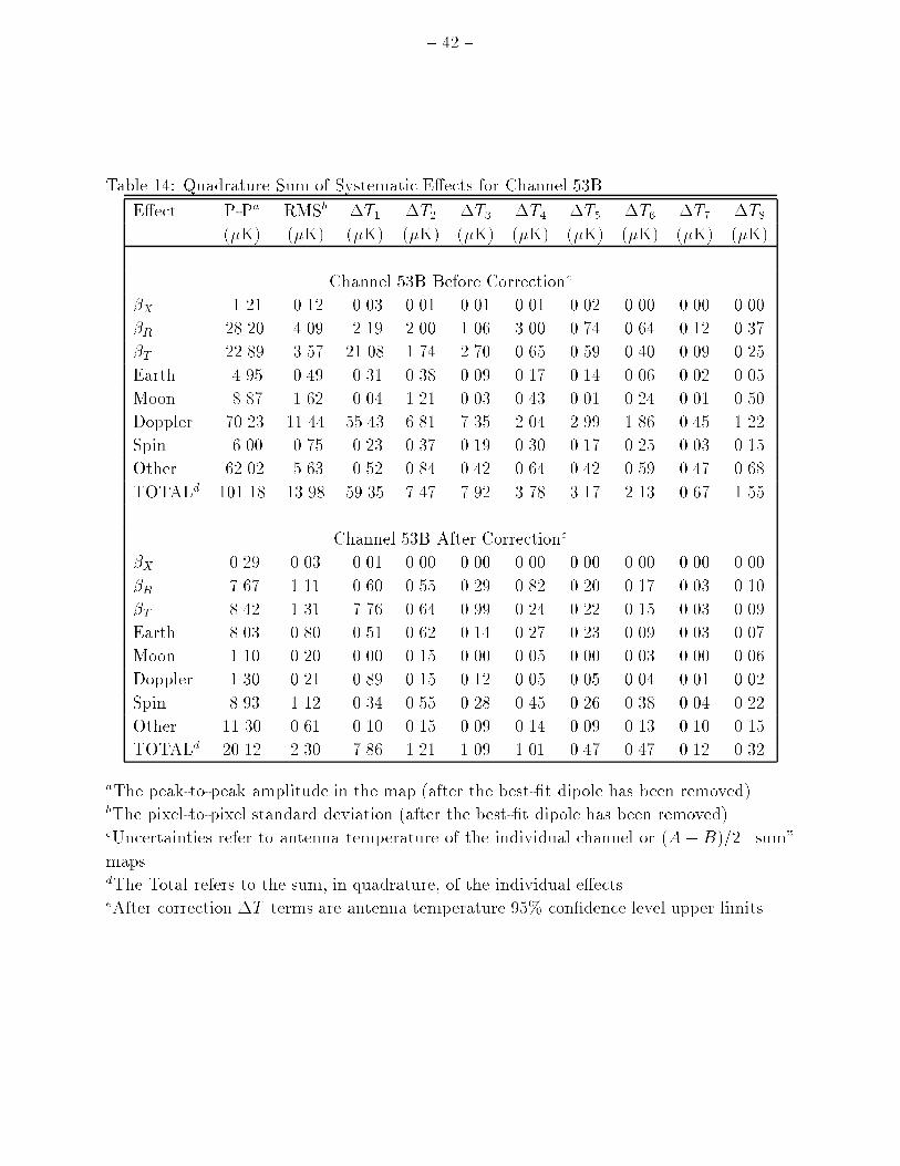
{ 42 {Table 14: Quadrature Sum of Systematic E�ects for Channel 53BE�ect P-Pa RMSb �T1 �T2 �T3 �T4 �T5 �T6 �T7 �T8(�K) (�K) (�K) (�K) (�K) (�K) (�K) (�K) (�K) (�K)Channel 53B Before Correctionc�X 1.21 0.12 0.03 0.01 0.01 0.01 0.02 0.00 0.00 0.00�R 28.20 4.09 2.19 2.00 1.06 3.00 0.74 0.64 0.12 0.37�T 22.89 3.57 21.08 1.74 2.70 0.65 0.59 0.40 0.09 0.25Earth 4.95 0.49 0.31 0.38 0.09 0.17 0.14 0.06 0.02 0.05Moon 8.87 1.62 0.04 1.21 0.03 0.43 0.01 0.24 0.01 0.50Doppler 70.23 11.44 55.43 6.81 7.35 2.04 2.99 1.86 0.45 1.22Spin 6.00 0.75 0.23 0.37 0.19 0.30 0.17 0.25 0.03 0.15Other 62.02 5.63 0.52 0.84 0.42 0.64 0.42 0.59 0.47 0.68TOTALd 101.18 13.98 59.35 7.47 7.92 3.78 3.17 2.13 0.67 1.55Channel 53B After Correctione�X 0.29 0.03 0.01 0.00 0.00 0.00 0.00 0.00 0.00 0.00�R 7.67 1.11 0.60 0.55 0.29 0.82 0.20 0.17 0.03 0.10�T 8.42 1.31 7.76 0.64 0.99 0.24 0.22 0.15 0.03 0.09Earth 8.03 0.80 0.51 0.62 0.14 0.27 0.23 0.09 0.03 0.07Moon 1.10 0.20 0.00 0.15 0.00 0.05 0.00 0.03 0.00 0.06Doppler 1.30 0.21 0.89 0.15 0.12 0.05 0.05 0.04 0.01 0.02Spin 8.93 1.12 0.34 0.55 0.28 0.45 0.26 0.38 0.04 0.22Other 11.30 0.61 0.10 0.15 0.09 0.14 0.09 0.13 0.10 0.15TOTALd 20.12 2.30 7.86 1.21 1.09 1.01 0.47 0.47 0.12 0.32aThe peak-to-peak amplitude in the map (after the best-�t dipole has been removed).bThe pixel-to-pixel standard deviation (after the best-�t dipole has been removed).cUncertainties refer to antenna temperature of the individual channel or (A+ B)=2 \sum"maps.dThe Total refers to the sum, in quadrature, of the individual e�ects.eAfter correction �T terms are antenna temperature 95% con�dence level upper limits.

{ 43 {Table 15: Quadrature Sum of Systematic E�ects for Channel 90AE�ect P-Pa RMSb �T1 �T2 �T3 �T4 �T5 �T6 �T7 �T8(�K) (�K) (�K) (�K) (�K) (�K) (�K) (�K) (�K) (�K)Channel 90A Before Correctionc�X 3.92 0.29 0.22 0.01 0.05 0.02 0.09 0.02 0.01 0.01�R 91.13 13.34 7.05 6.52 3.45 9.84 2.42 1.97 0.42 1.21�T 36.45 5.77 33.87 2.81 4.37 1.06 0.96 0.63 0.16 0.43Earth 3.58 0.41 0.29 0.31 0.07 0.14 0.12 0.07 0.02 0.03Moon 10.03 1.88 0.08 1.41 0.04 0.51 0.02 0.32 0.01 0.59Doppler 61.79 10.07 48.56 5.98 6.49 1.82 2.63 1.56 0.45 1.11Spin 6.00 0.75 0.23 0.37 0.19 0.30 0.17 0.25 0.03 0.15Other 73.32 7.85 1.59 0.77 0.63 0.61 0.45 0.55 0.43 0.62TOTALd 137.81 19.46 59.65 9.43 8.57 10.10 3.74 2.69 0.77 1.91Channel 90A After Correctione�X 1.03 0.08 0.06 0.00 0.01 0.01 0.02 0.01 0.00 0.00�R 13.30 1.95 1.03 0.95 0.50 1.44 0.35 0.29 0.06 0.18�T 13.41 2.12 12.47 1.03 1.61 0.39 0.35 0.23 0.06 0.16Earth 9.05 1.03 0.73 0.78 0.17 0.36 0.30 0.17 0.04 0.07Moon 1.64 0.31 0.01 0.23 0.01 0.08 0.00 0.05 0.00 0.10Doppler 2.54 0.42 1.94 0.26 0.26 0.08 0.11 0.06 0.02 0.05Spin 11.45 1.43 0.44 0.70 0.36 0.58 0.33 0.48 0.05 0.28Other 8.19 0.61 0.24 0.09 0.10 0.09 0.09 0.08 0.06 0.09TOTALd 25.44 3.47 12.69 1.79 1.75 1.64 0.68 0.64 0.13 0.40aThe peak-to-peak amplitude in the map (after the best-�t dipole has been removed).bThe pixel-to-pixel standard deviation (after the best-�t dipole has been removed).cUncertainties refer to antenna temperature of the individual channel or (A+ B)=2 \sum"maps.dThe Total refers to the sum, in quadrature, of the individual e�ects.eAfter correction �T terms are antenna temperature 95% con�dence level upper limits.

{ 44 {Table 16: Quadrature Sum of Systematic E�ects for Channel 90BE�ect P-Pa RMSb �T1 �T2 �T3 �T4 �T5 �T6 �T7 �T8(�K) (�K) (�K) (�K) (�K) (�K) (�K) (�K) (�K) (�K)Channel 90B Before Correctionc�X 0.12 0.01 0.01 0.00 0.00 0.00 0.00 0.00 0.00 0.00�R 10.18 1.50 0.79 0.73 0.39 1.10 0.27 0.22 0.05 0.14�T 19.91 3.14 18.42 1.53 2.38 0.58 0.52 0.34 0.09 0.23Earth 3.97 0.41 0.30 0.31 0.07 0.14 0.11 0.05 0.02 0.04Moon 11.17 2.07 0.08 1.54 0.04 0.56 0.02 0.32 0.01 0.64Doppler 62.48 10.08 48.55 5.98 6.50 1.82 2.64 1.56 0.46 1.11Spin 6.00 0.75 0.23 0.37 0.19 0.30 0.17 0.25 0.03 0.15Other 67.54 6.31 1.82 0.78 0.69 0.61 0.47 0.55 0.43 0.63TOTALd 95.61 12.59 51.97 6.47 6.97 2.38 2.75 1.75 0.64 1.46Channel 90B After Correctione�X 0.54 0.04 0.02 0.00 0.01 0.00 0.01 0.00 0.00 0.00�R 4.07 0.60 0.32 0.29 0.15 0.44 0.11 0.09 0.02 0.05�T 9.24 1.46 8.55 0.71 1.10 0.27 0.24 0.16 0.04 0.11Earth 7.32 0.76 0.56 0.58 0.13 0.26 0.21 0.09 0.03 0.08Moon 1.81 0.34 0.01 0.25 0.01 0.09 0.00 0.05 0.00 0.10Doppler 1.84 0.30 1.36 0.19 0.18 0.06 0.08 0.05 0.01 0.03Spin 5.70 0.71 0.22 0.35 0.18 0.29 0.16 0.24 0.02 0.14Other 8.45 0.62 0.21 0.09 0.09 0.09 0.09 0.08 0.06 0.09TOTALd 16.32 2.04 8.68 1.07 1.15 0.66 0.39 0.33 0.09 0.25aThe peak-to-peak amplitude in the map (after the best-�t dipole has been removed).bThe pixel-to-pixel standard deviation (after the best-�t dipole has been removed).cUncertainties refer to antenna temperature of the individual channel or (A+ B)=2 \sum"maps.dThe Total refers to the sum, in quadrature, of the individual e�ects.eAfter correction �T terms are antenna temperature 95% con�dence level upper limits.

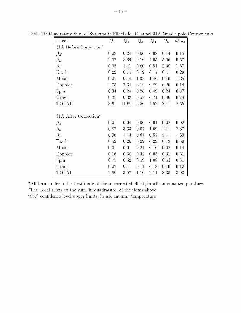
{ 45 {Table 17: Quadrature Sum of Systematic E�ects for Channel 31A Quadrupole ComponentsE�ect Q1 Q2 Q3 Q4 Q5 Qrms31A Before Correctiona�X 0.03 0.24 0.00 0.08 0.14 0.15�R 2.07 8.69 0.16 4.05 5.06 5.67�T 0.95 1.41 0.80 0.51 2.38 1.57Earth 0.29 0.15 0.12 0.17 0.41 0.28Moon 0.05 0.14 1.93 1.46 0.16 1.25Doppler 2.75 7.64 6.19 0.89 6.20 6.14Spin 0.34 0.24 0.26 0.49 0.24 0.37Other 0.25 0.82 0.53 0.71 0.86 0.78TOTALb 3.61 11.69 6.56 4.52 8.41 8.6531A After Correctionc�X 0.01 0.04 0.00 0.01 0.02 0.02�R 0.87 3.63 0.07 1.69 2.11 2.37�T 0.96 1.43 0.81 0.52 2.41 1.59Earth 0.52 0.26 0.22 0.29 0.73 0.50Moon 0.01 0.01 0.21 0.16 0.02 0.14Doppler 0.16 0.38 0.32 0.05 0.31 0.31Spin 0.75 0.52 0.59 1.08 0.53 0.81Other 0.03 0.11 0.11 0.13 0.10 0.12TOTAL 1.59 3.97 1.10 2.11 3.35 3.03aAll terms refer to best estimate of the uncorrected e�ect, in �K antenna temperaturebThe Total refers to the sum, in quadrature, of the items abovec95% con�dence level upper limits, in �K antenna temperature

{ 46 {Table 18: Quadrature Sum of Systematic E�ects for Channel 31B Quadrupole ComponentsE�ect Q1 Q2 Q3 Q4 Q5 Qrms31B Before Correctiona�X 0.06 0.12 0.02 0.00 0.08 0.08�R 7.42 10.22 1.11 0.54 7.78 7.44�T 0.12 0.55 0.33 0.08 0.79 0.53Earth 0.38 0.18 0.13 0.19 0.44 0.32Moon 0.09 0.06 1.95 1.45 0.18 1.26Doppler 1.72 10.67 9.09 2.56 3.91 7.67Spin 0.34 0.24 0.26 0.49 0.24 0.37Other 0.43 0.84 0.39 0.89 0.86 0.82TOTALb 7.64 14.82 9.38 3.16 8.80 10.8231B After Correctionc�X 0.07 0.13 0.02 0.00 0.08 0.09�R 3.83 5.28 0.57 0.28 4.01 3.84�T 0.38 1.72 1.03 0.24 2.47 1.66Earth 0.71 0.34 0.24 0.35 0.81 0.59Moon 0.01 0.01 0.21 0.15 0.02 0.13Doppler 0.09 0.49 0.45 0.13 0.19 0.36Spin 1.61 1.12 1.26 2.32 1.13 1.75Other 0.08 0.15 0.10 0.16 0.12 0.14TOTALb 4.23 5.70 1.81 2.39 4.92 4.59aAll terms refer to best estimate of the uncorrected e�ect, in �K antenna temperaturebThe Total refers to the sum, in quadrature, of the items abovec95% con�dence level upper limits, in �K antenna temperature

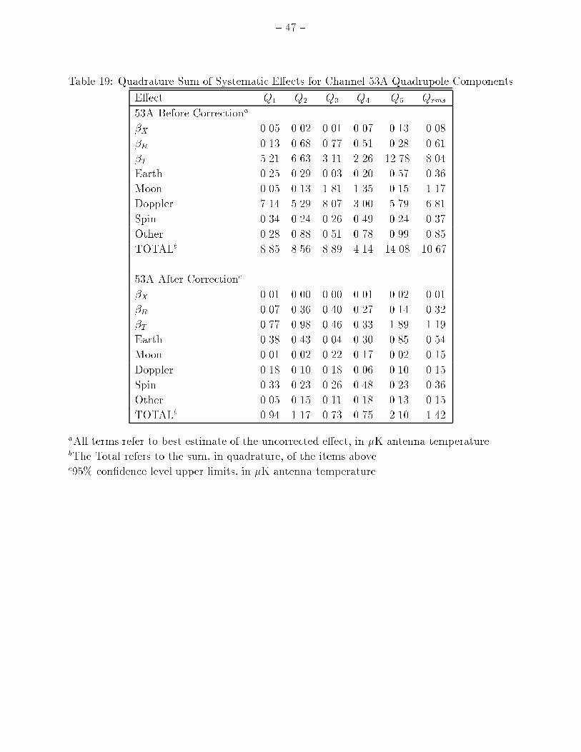
{ 47 {Table 19: Quadrature Sum of Systematic E�ects for Channel 53A Quadrupole ComponentsE�ect Q1 Q2 Q3 Q4 Q5 Qrms53A Before Correctiona�X 0.05 0.02 0.01 0.07 0.13 0.08�R 0.13 0.68 0.77 0.51 0.28 0.61�T 5.21 6.63 3.11 2.26 12.78 8.04Earth 0.25 0.29 0.03 0.20 0.57 0.36Moon 0.05 0.13 1.81 1.35 0.15 1.17Doppler 7.14 5.29 8.07 3.00 5.79 6.81Spin 0.34 0.24 0.26 0.49 0.24 0.37Other 0.28 0.88 0.51 0.78 0.99 0.85TOTALb 8.85 8.56 8.89 4.14 14.08 10.6753A After Correctionc�X 0.01 0.00 0.00 0.01 0.02 0.01�R 0.07 0.36 0.40 0.27 0.14 0.32�T 0.77 0.98 0.46 0.33 1.89 1.19Earth 0.38 0.43 0.04 0.30 0.85 0.54Moon 0.01 0.02 0.22 0.17 0.02 0.15Doppler 0.18 0.10 0.18 0.06 0.10 0.15Spin 0.33 0.23 0.26 0.48 0.23 0.36Other 0.05 0.15 0.11 0.18 0.13 0.15TOTALb 0.94 1.17 0.73 0.75 2.10 1.42aAll terms refer to best estimate of the uncorrected e�ect, in �K antenna temperaturebThe Total refers to the sum, in quadrature, of the items abovec95% con�dence level upper limits, in �K antenna temperature

{ 48 {Table 20: Quadrature Sum of Systematic E�ects for Channel 53B Quadrupole ComponentsE�ect Q1 Q2 Q3 Q4 Q5 Qrms53B Before Correctiona�X 0.00 0.00 0.00 0.00 0.01 0.01�R 0.43 2.24 2.52 1.66 0.90 2.00�T 1.13 1.44 0.68 0.49 2.77 1.74Earth 0.28 0.31 0.02 0.20 0.59 0.38Moon 0.06 0.13 1.86 1.39 0.15 1.21Doppler 7.14 5.28 8.08 3.01 5.78 6.81Spin 0.34 0.24 0.26 0.49 0.24 0.37Other 0.27 0.88 0.51 0.79 0.97 0.84TOTALb 7.26 5.99 8.71 3.86 6.58 7.4753B After Correctionc�X 0.00 0.00 0.00 0.00 0.00 0.00�R 0.12 0.61 0.68 0.45 0.25 0.55�T 0.42 0.53 0.25 0.18 1.02 0.64Earth 0.45 0.49 0.04 0.33 0.96 0.62Moon 0.01 0.02 0.23 0.17 0.02 0.15Doppler 0.18 0.10 0.18 0.06 0.10 0.15Spin 0.50 0.35 0.39 0.73 0.35 0.55Other 0.05 0.15 0.12 0.18 0.13 0.16TOTALb 0.82 1.02 0.89 0.97 1.48 1.21aAll terms refer to best estimate of the uncorrected e�ect, in �K antenna temperaturebThe Total refers to the sum, in quadrature, of the items abovec95% con�dence level upper limits, in �K antenna temperature

{ 49 {Table 21: Quadrature Sum of Systematic E�ects for Channel 90A Quadrupole ComponentsE�ect Q1 Q2 Q3 Q4 Q5 Qrms90A Before Correctiona�X 0.02 0.01 0.00 0.01 0.02 0.01�R 1.50 7.21 8.27 5.39 2.88 6.52�T 1.81 2.32 1.09 0.78 4.47 2.81Earth 0.23 0.25 0.03 0.16 0.48 0.31Moon 0.06 0.15 2.18 1.62 0.18 1.41Doppler 6.26 4.64 7.08 2.66 5.09 5.98Spin 0.34 0.24 0.26 0.49 0.24 0.37Other 0.24 0.79 0.56 0.71 0.88 0.77TOTALb 6.71 8.92 11.17 6.34 7.43 9.4390A After Correctionc�X 0.01 0.00 0.00 0.00 0.00 0.00�R 0.22 1.05 1.21 0.79 0.42 0.95�T 0.67 0.85 0.40 0.29 1.64 1.03Earth 0.59 0.64 0.07 0.39 1.21 0.78Moon 0.01 0.03 0.36 0.27 0.03 0.23Doppler 0.28 0.19 0.31 0.11 0.21 0.26Spin 0.65 0.45 0.50 0.93 0.45 0.70Other 0.03 0.09 0.08 0.10 0.09 0.09TOTALb 1.16 1.58 1.45 1.35 2.15 1.79aAll terms refer to best estimate of the uncorrected e�ect, in �K antenna temperaturebThe Total refers to the sum, in quadrature, of the items abovec95% con�dence level upper limits, in �K antenna temperature

{ 50 {Table 22: Quadrature Sum of Systematic E�ects for Channel 90B Quadrupole ComponentsE�ect Q1 Q2 Q3 Q4 Q5 Qrms90B Before Correctiona�X 0.00 0.00 0.00 0.00 0.00 0.00�R 0.17 0.81 0.92 0.61 0.32 0.73�T 0.98 1.26 0.59 0.42 2.43 1.53Earth 0.23 0.26 0.02 0.16 0.49 0.31Moon 0.07 0.17 2.38 1.77 0.20 1.54Doppler 6.27 4.64 7.07 2.66 5.09 5.98Spin 0.34 0.24 0.26 0.49 0.24 0.37Other 0.23 0.81 0.58 0.70 0.86 0.78TOTALb 6.37 4.96 7.57 3.40 5.74 6.4790B After Correctionc�X 0.00 0.00 0.00 0.00 0.00 0.00�R 0.07 0.32 0.37 0.24 0.13 0.29�T 0.46 0.58 0.27 0.20 1.13 0.71Earth 0.42 0.47 0.04 0.30 0.90 0.58Moon 0.01 0.03 0.39 0.29 0.03 0.25Doppler 0.21 0.14 0.23 0.08 0.15 0.19Spin 0.32 0.22 0.25 0.46 0.23 0.35Other 0.03 0.09 0.08 0.10 0.08 0.09TOTALb 0.73 0.86 0.69 0.71 1.48 1.07aAll terms refer to best estimate of the uncorrected e�ect, in �K antenna temperaturebThe Total refers to the sum, in quadrature, of the items abovec95% con�dence level upper limits, in �K antenna temperature

{ 51 {Table 23: RMS Thermodynamic Temperature FluctuationsData set bcut 7� RMS (unit weighting) 10� RMS (unit weighting)Sum Di� Sky Sum Di� Sky(�) (�K) (�K) (�K) (�K) (�K) (�K)31 Yr 1 10 415.1 394.8 128:1 139.0 101.9 94:520 409.6 401.8 80:0 110.0 105.7 30:230 417.1 411.9 65:7 106.7 107.9 0:040 421.8 418.8 50:0 112.7 108.2 31:631 Yr 2 10 460.2 439.6 136:4 143.9 113.0 89:120 464.6 449.8 116:5 124.1 115.6 45:330 474.3 462.5 104:9 123.5 116.3 41:640 488.6 474.4 116:9 121.6 124.7 0:031 2 Yr 10 310.5 290.8 109:0 � 27:5 117.5 76.0 89:7 � 9:520 303.6 295.7 69:2 � 29:5 85.3 77.6 35:5 � 11:230 306.8 305.0 34:0 � 31:3 80.9 78.1 21:1 � 13:240 314.0 310.0 49:8 � 34:9 83.7 78.8 27:9 � 15:553 Yr 1 10 160.7 152.0 52:3 56.0 38.2 41:020 158.2 151.6 45:2 49.3 37.7 31:730 159.0 151.9 47:1 48.9 38.4 30:340 159.9 153.3 45:4 50.3 39.4 31:253 Yr 2 10 162.7 149.8 63:5 57.5 38.6 42:620 160.6 149.3 59:0 50.2 38.6 32:230 158.6 149.1 54:2 49.9 39.4 30:640 156.9 147.5 53:4 47.4 38.9 27:153 2 Yr 10 118.9 105.9 54:2 � 6:4 50.2 26.7 42:5 � 2:220 115.2 106.3 44:4 � 7:5 42.1 26.9 32:4 � 2:530 114.6 105.8 43:9 � 9:0 40.9 27.2 30:5 � 2:740 115.1 103.8 49:7 � 10:9 40.6 27.2 30:2 � 3:290 Yr 1 10 243.4 243.0 13:9 70.3 61.4 34:320 242.5 243.7 0:0 65.7 64.0 14:930 243.1 244.1 0:0 67.2 62.4 24:940 241.8 245.2 0:0 66.6 61.6 25:390 Yr 2 10 247.7 244.7 38:5 75.1 64.4 38:520 245.1 244.6 15:7 68.7 64.5 23:830 243.0 243.9 0:0 69.7 61.2 33:340 242.0 243.9 0:0 67.8 62.3 26:890 2 Yr 10 175.5 174.4 20:0 � 10:1 59.0 44.5 38:7 � 3:220 173.3 173.8 0:0 � 11:9 52.8 46.1 25:7 � 3:830 174.5 171.8 30:2 � 14:3 54.4 41.8 34:8 � 4:140 172.8 173.1 0:0 � 17:4 54.4 42.6 33:9 � 4:9

{ 52 {Table 24: RMS Thermodynamic Temperature Fluctuations with Galaxy RemovedData set bcut 7� RMS (unit weighting) 10� RMS (unit weighting)Sum Di� Sky Sum Di� Sky(�) (�K) (�K) (�K) (�K) (�K) (�K)Comb Yr 1 10 276.3 267.8 68:0 73.6 67.2 30:020 277.8 271.0 61:1 73.5 67.9 28:030 283.6 273.5 74:9 76.7 70.4 30:440 285.2 277.9 64:5 79.3 71.5 34:4Comb Yr 2 10 299.2 283.1 96:7 81.1 72.1 37:120 304.0 286.4 102:0 80.2 73.8 31:330 307.2 291.0 98:4 81.6 74.3 33:740 313.6 292.4 113:4 82.3 75.4 33:0Comb 2 Yr 10 201.9 194.0 55:7� 15:4 58.5 49.6 31:1 � 5:320 203.8 197.0 52:2� 17:0 57.6 51.2 26:4 � 6:230 206.0 199.1 53:2� 18:8 59.4 51.9 28:9 � 7:140 208.7 197.7 67:0� 21:8 60.5 52.5 30:1 � 8:4Subt Yr 1 10 227.2 223.1 42:9 63.5 55.5 30:820 227.7 226.3 25:0 62.5 57.0 25:830 231.7 228.7 37:2 64.8 58.3 28:440 232.1 230.5 27:7 67.5 58.7 33:2Subt Yr 2 10 242.3 232.5 68:2 68.9 58.4 36:520 245.0 233.6 74:0 67.0 58.4 32:830 247.1 236.3 72:1 67.9 57.7 35:840 251.4 236.1 86:1 67.8 57.7 35:6Subt 2 Yr 10 165.0 159.9 40:7� 11:9 51.7 40.0 32:8 � 4:020 165.8 161.7 36:7� 13:2 50.2 41.2 28:7 � 4:730 168.0 162.4 43:3� 14:9 51.3 40.1 32:1 � 5:440 169.4 161.9 49:8� 17:4 52.6 40.5 33:5 � 6:4

{ 53 {Table 25: Quadrupole Resultsa After Subtraction-Technique Galaxy RemovalQuad Year 1 Year 1 Year 2 Year 2 2 Year 2 YearComp Sum Di� Sum Di� Sum Di�Q1 9:7� 7:9 �10:1� 7:1 �9:4� 8:4 4:0 � 7:7 2:0� 6:5 �4:9� 5:5Q2 10:1 � 6:0 �2:1� 5:9 �2:0� 5:9 �6:6� 5:8 5:0� 4:0 �5:2� 3:9Q3 14:1 � 5:2 �0:1� 5:2 5:3 � 5:9 �1:7� 5:9 9:6� 4:0 �0:8� 4:0Q4 4:9� 7:6 14:3 � 6:7 2:2 � 8:0 �1:0� 7:1 2:9� 5:9 7:6 � 4:7Q5 4:9� 7:3 �1:5� 6:4 10:3 � 7:6 �5:1� 6:7 7:0� 5:9 �2:9� 4:7Qrms 10:6 8:7 7:5 4:8 6:9 5:5�2 12:6 6:7 4:1 2:3 9:1 5:6a Values are in thermodynamic �K. Uniform weighting of the map pixels was used. Theorder of the �t was truncated at ` = 2. A Galactic cut of 10� was applied. The kinematicquadrupole correction was applied. A 1.5% correction was applied to restore power lost bybeam dilution.Table 26: Quadrupole Resultsa After Combination-Technique Galaxy RemovalQuad Year 1 Year 1 Year 2 Year 2 2 Year 2 YearComp Sum Di� Sum Di� Sum Di�Q1 10:0 � 9:8 �14:6 � 9:2 �11:7� 10:7 4:2 � 10:1 2:0 � 7:4 �7:9� 6:5Q2 12:6 � 6:6 �1:7� 6:5 �1:2� 7:2 �5:4� 7:1 6:9 � 5:3 �5:0� 5:2Q3 13:6 � 6:4 1:2 � 6:4 9:1� 7:6 �2:3� 7:6 11:0 � 5:0 �0:8� 5:0Q4 0:4� 8:7 12:8 � 7:9 3:8� 9:3 �2:3� 8:6 1:0 � 7:0 6:6� 6:0Q5 7:1� 8:6 �2:7� 7:8 14:1� 9:3 �9:5� 8:5 10:1 � 6:9 �5:4� 5:8Qrms 11:2 9:5 10:3 6:2 8:6 6:2�2 9:9 5:4 5:1 2:2 8:8 4:5a Values are in thermodynamic �K. Uniform weighting of the map pixels was used. Theorder of the �t was truncated at ` = 2. A Galactic cut of 10� was applied. The kinematicquadrupole correction was applied. A 1.5% correction was applied to restore power lost bybeam dilution.

{ 54 {FIGURE CAPTIONSFigure 1: Mollweide projections of the full sky in Galactic coordinates with theGalactic center at the center of the maps and longitude increasing towards the left. Thedata are smoothed to an e�ective resolution of 10�. (a) The 31 GHz, 53 GHz, and 90 GHz(A+ B)=2 (sum) data, and (b) The 31 GHz, 53 GHz, and 90 GHz (A�B)=2 (di�erence)data.Figure 2: Azimuthal equal area projections of the dipole removed 53 GHz (A+B)=2(sum) data and the combination technique Galaxy-reduced data, smoothed to 10�. TheNorth Galactic polar cap is on the left, the South Galactic polar cap is on the right, andthe point where they meet is the Galactic center. ` = 90� is at the bottom of each projectedpolar cap.Figure 3: The two-point 53 GHz (A + B)=2 � 90 GHz (A + B)=2 cross correlationfunction with the dipole removed, for jbj > 20� in thermodynamic temperature units. Theerror bars on the individual points include only instrument noise. top: The two-point crosscorrelation with the quadrupole included. The shaded region is the 68% con�dence regionexpected from a 12.4 �K, n=1.6 spectrum of uctuations, including cosmic variance andinstrument noise. bottom: The two-point cross correlation with the quadrupole excluded.The shaded region is the 68% con�dence region expected from a 16.0 �K, n=1.2 spectrumof uctuations, including cosmic variance and instrument noise.Figure 4: Likelihood contours as a function of n and Qrms�PS for the data shownin Figure 3. The contours correspond to 68%, 95%, and 99.7% con�dence regions. Thesolid curves are with the quadrupole included, with the peak of the likelihood indicated by+. The dashed curves are with the quadrupole excluded, with the peak of the likelihoodindicated by *.Figure 5: Likelihood functions for the observed quadrupole amplitude Qrms in thesubtraction technique CMB map. (a) The likelihood of Qrms using only the �rst year data.The solid curve is for the (A+ B)=2 sum data and the dashed curve is for the (A�B)=2di�erence data. (b) The same as (a), but for the second year of data. (c) The same as (a),but for the �rst two years of data combined.

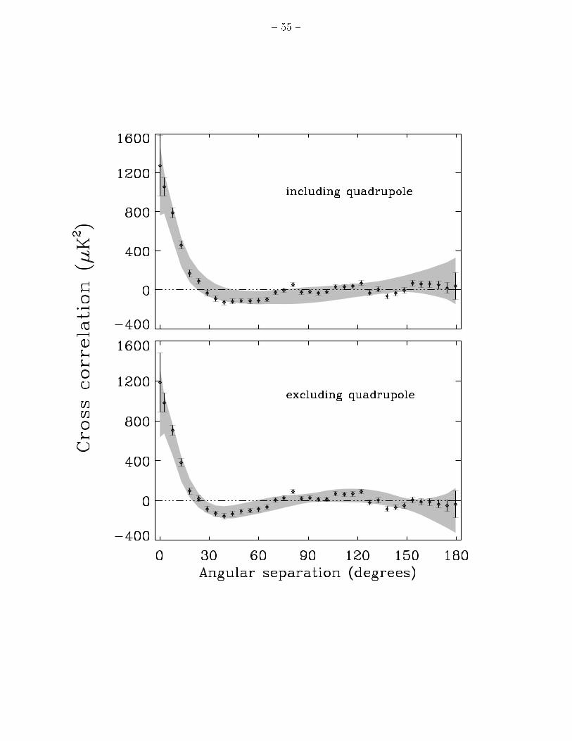
{ 55 {

{ 56 {

{ 57 {