Embed Size (px)
Citation preview

ALTERNATIVE PORTFOLIO METHODS
by
RUANMIN CAO
A thesis submitted to the University of Birmingham for the degree of
DOCTOR OF PHILOSOPHY
Department of Economics
Business School
College of Social Science
University of Birmingham
April 2015

University of Birmingham Research Archive
e-theses repository This unpublished thesis/dissertation is copyright of the author and/or third parties. The intellectual property rights of the author or third parties in respect of this work are as defined by The Copyright Designs and Patents Act 1988 or as modified by any successor legislation. Any use made of information contained in this thesis/dissertation must be in accordance with that legislation and must be properly acknowledged. Further distribution or reproduction in any format is prohibited without the permission of the copyright holder.

Alternative Portfolio Methods
Abstract
Portfolio optimization in an uncertain environment has great practical
value in investment decision process. But this area is highly fragmented
due to fast evolution of market structure and changing investor behavior.
In this dissertation, four methods are investigated/designed to explore
their efficiency under different circumstances.
Parametric portfolio decomposes weights by a set of factors whose coef-
ficients are uniquely determined via maximizing utility function. A robust
bootstrap method is proposed to assist factor selection. If investors ex-
hibit asymmetric aversion of tail risk, pessimistic models on Choquet util-
ity maximization and coherent risk measures acquire superiority. A new
hybrid method that inherits advantage of parameterization and tail risk
minimization is designed. Mean-variance, which is optimal with elliptical
return distribution, should be employed in the case of capital allocation to
trading strategies. Nonparametric classifiers may enhance homogeneity of
inputs before feeding the optimizer. Traditional factor portfolio can be ex-
tended to functional settings by applying FPCA to return curves sorted
by factors. Diversification is always achieved by mixing with detected
nonlinear components.
This research contributes to existing literature on portfolio choice in
three-folds: strength and weakness of each method is clarified; new models
that outperform traditional approaches are developed; empirical studies
are used to facilitate comparison.
2

CONTENTS Alternative Portfolio Methods
Contents
1 Introduction 11
1.1 Mean-Variance . . . . . . . . . . . . . . . . . . . . . . . . . . . . 12
1.2 Minimizing Tail Risk . . . . . . . . . . . . . . . . . . . . . . . . . 16
1.3 Portfolio Parameterization . . . . . . . . . . . . . . . . . . . . . . 19
1.4 Pricing Risk Factors . . . . . . . . . . . . . . . . . . . . . . . . . 21
2 Portfolio Parameterization 23
2.1 Background . . . . . . . . . . . . . . . . . . . . . . . . . . . . . . 23
2.2 Model Configuration . . . . . . . . . . . . . . . . . . . . . . . . . 26
2.2.1 Basic Model . . . . . . . . . . . . . . . . . . . . . . . . . . 26
2.2.2 Some Utility Functionals . . . . . . . . . . . . . . . . . . . 28
2.2.3 Extensions . . . . . . . . . . . . . . . . . . . . . . . . . . 30
2.3 Measuring Predictive/Profitable Ability . . . . . . . . . . . . . . 37
2.4 Performance on FTSE100 . . . . . . . . . . . . . . . . . . . . . . 41
2.5 Concluding Remarks . . . . . . . . . . . . . . . . . . . . . . . . . 49
2.6 Appendix . . . . . . . . . . . . . . . . . . . . . . . . . . . . . . . 52
2.6.1 Technical Indicators . . . . . . . . . . . . . . . . . . . . . 52
3 On Investor’s Pessmism 56
3.1 Background . . . . . . . . . . . . . . . . . . . . . . . . . . . . . . 56
3.2 Pessimistic Models . . . . . . . . . . . . . . . . . . . . . . . . . . 58
3.2.1 Quadratic Utility Function and Coherent Risk Measure . 58
3

CONTENTS Alternative Portfolio Methods
3.2.2 Optimization of Conditional Value-at-Risk and Pessimistic
Portfolio . . . . . . . . . . . . . . . . . . . . . . . . . . . . 60
3.2.3 Parametric Pessimistic Portfolio . . . . . . . . . . . . . . 66
3.2.4 Efficient Frontier and Maximizing Reward/Risk Ratio . . 70
3.3 Empirical Study on Global Indices Portfolio . . . . . . . . . . . . 72
3.3.1 Data . . . . . . . . . . . . . . . . . . . . . . . . . . . . . . 72
3.3.2 Simulation Results . . . . . . . . . . . . . . . . . . . . . . 74
3.4 Discussion . . . . . . . . . . . . . . . . . . . . . . . . . . . . . . . 78
3.4.1 Tail Distribution Stationarity, Overconcentration and Boot-
strap . . . . . . . . . . . . . . . . . . . . . . . . . . . . . . 78
3.4.2 Quantile Analysis . . . . . . . . . . . . . . . . . . . . . . . 81
3.4.3 Out-of-sample Degeneration . . . . . . . . . . . . . . . . . 82
3.4.4 Profitability and Resistence to Market Friction . . . . . . 83
3.5 Concluding Remarks . . . . . . . . . . . . . . . . . . . . . . . . . 88
3.6 Appendix . . . . . . . . . . . . . . . . . . . . . . . . . . . . . . . 90
3.6.1 Computational aspects of pessimistic models . . . . . . . 90
3.7 Tables and Figures . . . . . . . . . . . . . . . . . . . . . . . . . . 95
4 Mean-Variance on Heterogeneous Sample 105
4.1 Background . . . . . . . . . . . . . . . . . . . . . . . . . . . . . . 105
4.2 Model Configuration . . . . . . . . . . . . . . . . . . . . . . . . . 107
4.3 Predictability and Trading Strategy Design . . . . . . . . . . . . 110
4.4 Nonparametric Classifier Filtering . . . . . . . . . . . . . . . . . 113
4.4.1 K Nearest Neighbors (KNN) . . . . . . . . . . . . . . . . 113
4

CONTENTS Alternative Portfolio Methods
4.4.2 Discriminant Adaptive Nearest Neighbor Classification (DANN)114
4.5 Data Input and Implementation . . . . . . . . . . . . . . . . . . . 115
4.6 Performance . . . . . . . . . . . . . . . . . . . . . . . . . . . . . . 117
4.7 Analysis . . . . . . . . . . . . . . . . . . . . . . . . . . . . . . . . 117
4.7.1 Reality Check on Strategy Profitability . . . . . . . . . . 117
4.7.2 Robustness . . . . . . . . . . . . . . . . . . . . . . . . . . 118
4.8 Concluding Remarks . . . . . . . . . . . . . . . . . . . . . . . . . 119
4.9 Appendix . . . . . . . . . . . . . . . . . . . . . . . . . . . . . . . 120
5 Functional Predictability of Factors and Basis Portfolios 128
5.1 Background . . . . . . . . . . . . . . . . . . . . . . . . . . . . . . 128
5.1.1 Risk Factors . . . . . . . . . . . . . . . . . . . . . . . . . 128
5.1.2 Empirical Studies on Emerging Stock Market . . . . . . . 131
5.1.3 Functional Data Analysis . . . . . . . . . . . . . . . . . . 133
5.2 Methodology . . . . . . . . . . . . . . . . . . . . . . . . . . . . . 136
5.2.1 Inference for functional linear dependence . . . . . . . . . 136
5.2.2 Functional dependence forecast model . . . . . . . . . . . 140
5.2.3 Constructing Portfolio with Basis Functions . . . . . . . . 143
5.3 Experiment . . . . . . . . . . . . . . . . . . . . . . . . . . . . . . 146
5.3.1 Implementation Procedure . . . . . . . . . . . . . . . . . . 146
5.3.2 Data Sample . . . . . . . . . . . . . . . . . . . . . . . . . 147
5.3.3 Data Reformat . . . . . . . . . . . . . . . . . . . . . . . . 148
5.3.4 Cross-sectional Momentum . . . . . . . . . . . . . . . . . 149
5.4 Empirical Results . . . . . . . . . . . . . . . . . . . . . . . . . . . 150
5

CONTENTS Alternative Portfolio Methods
5.4.1 FPC of Return Curve . . . . . . . . . . . . . . . . . . . . 150
5.5 Portfolio Performance . . . . . . . . . . . . . . . . . . . . . . . . 151
5.5.1 Predicting Scores . . . . . . . . . . . . . . . . . . . . . . . 154
5.6 Concluding Remarks . . . . . . . . . . . . . . . . . . . . . . . . . 156
5.7 Appendix . . . . . . . . . . . . . . . . . . . . . . . . . . . . . . . 158
6 Conclusion 173
6
LIST OF FIGURES Alternative Portfolio Methods
List of Figures
2.1 Parametric Portfolio Performance ON FT100 . . . . . . . . . . . 43
2.2 Rolling Breakeven Transation Cost . . . . . . . . . . . . . . . . . 46
2.3 ROLLING TURNOVER . . . . . . . . . . . . . . . . . . . . . . . 47
2.4 ROLLING CV aR0.05 (WINDOW LENGTH = 100) . . . . . . . 48
2.5 QQPLOT: Parametric Portfolio vs Normality . . . . . . . . . . . 50
2.6 QQPLOT: Equal Weights vs Normality . . . . . . . . . . . . . . 50
2.7 QQPLOT: Parametric Portfolio vs Equal Weights . . . . . . . . 51
2.8 Out-of-Sample Degeneracy . . . . . . . . . . . . . . . . . . . . . . 51
3.1 Efficient Frontier . . . . . . . . . . . . . . . . . . . . . . . . . . . 72
3.2 100 weeks rolling CVaRα on benchmark return. τ = 0.1 . . . . . 79
3.3 QQ Plot of empirical return distribution vs normal distribution. 99
3.4 QQ Plot Comparison between two simulated returns. . . . . . . . 100
3.5 Out-of-Sample Degeneracy of three active portfolio schemes. . . 101
3.6 Portfolio Composition with Various Target Return on December.
2006. . . . . . . . . . . . . . . . . . . . . . . . . . . . . . . . . . . 102
3.7 Bootstrap Portfolio Composition with Various Target Return on
December. 2006. . . . . . . . . . . . . . . . . . . . . . . . . . . . 103
3.8 Portfolio profitability resistence to market friction. . . . . . . . . 104
4.1 Mean-Variance Efficient Frontier . . . . . . . . . . . . . . . . . . 121
4.2 Portfolio Performance . . . . . . . . . . . . . . . . . . . . . . . . 121
4.3 Out-of-Sample Degeneracy . . . . . . . . . . . . . . . . . . . . . . 122
4.4 Out-of-Sample Degeneracy . . . . . . . . . . . . . . . . . . . . . . 123
7

LIST OF FIGURES Alternative Portfolio Methods
5.1 The First and Second Moments of Returns on Each Group Sorted
by Momentum Factor . . . . . . . . . . . . . . . . . . . . . . . . 152
5.2 Simulation Platform designed for retrieving data from database,
sorting stocks based on factors and grouping returns . . . . . . . 167
5.3 Basis Functions derived from FPCA on cross-sectional return
curve. Look-back period is one month h = 4. . . . . . . . . . . . 168
5.4 Basis Functions derived from FPCA on cross-sectional return
curve. Look-back period is two months h = 8. . . . . . . . . . . . 169
5.5 Basis Functions derived from FPCA on cross-sectional return
curve. Look-back period is one quarter h = 12. . . . . . . . . . . 170
5.6 Basis Functions derived from FPCA on cross-sectional return
curve. Look-back period is half year h = 26. . . . . . . . . . . . . 171
5.7 Basis Functions derived from FPCA on cross-sectional return
curve. Look-back period is one year h = 52. . . . . . . . . . . . . 172
8
LIST OF TABLES Alternative Portfolio Methods
List of Tables
2.1 White p-value of Five Technical Trading Rule Systems . . . . . . 43
2.2 Optimal Technical Trading Rule under Sharpe Ratio Criterion . 44
2.3 Parametric Portfolio Performance Statistics . . . . . . . . . . . . 45
2.4 MOMENTS OF DEGENERATION DISTRIBUTION . . . . . . 45
3.1 Details of Indices Data Set . . . . . . . . . . . . . . . . . . . . . 75
3.2 Simulation Result From 2001 to 2012 . . . . . . . . . . . . . . . . 77
3.3 Descriptive Statistics of Country Indices . . . . . . . . . . . . . . 95
3.4 Out-of-Sample Performance of Boostrap Pessimistic Portfolio,
January 2007 - December 2012 . . . . . . . . . . . . . . . . . . . 96
3.5 Out-of-Sample Degeneracy Moments . . . . . . . . . . . . . . . . 97
3.6 Breakeven Transaction Cost . . . . . . . . . . . . . . . . . . . . . 98
4.1 Contracts Covered in MSCI . . . . . . . . . . . . . . . . . . . . . 120
4.2 Descriptive Statistics of Continuous Futures Index . . . . . . . . 124
4.3 Momentum Strategy Performance . . . . . . . . . . . . . . . . . . 125
4.4 Reality Check p-Value . . . . . . . . . . . . . . . . . . . . . . . . 126
4.5 Statistics of Performance . . . . . . . . . . . . . . . . . . . . . . . 127
4.6 Out-of-Sample Degeneration Moments . . . . . . . . . . . . . . . 127
5.1 p−value of Dependency Test . . . . . . . . . . . . . . . . . . . . . 155
5.2 Summary of Test on Predicting Scores (Sign of Index Return) . . 158
5.3 Summary of Test on Predicting Scores (Index Return) . . . . . . 159
5.4 Summary of Test on Predicting Scores (Sign of Index Return) . . 160
5.5 Summary of Test on Predicting Scores (Index Return) . . . . . . 161
9

LIST OF TABLES Alternative Portfolio Methods
5.6 Summary of Test on Predicting Scores (Volatility) . . . . . . . . 162
5.7 Summary of Test on Predicting Scores (Volatility) . . . . . . . . 163
5.8 Summary of Test on Predicting Scores (Kurtosis) . . . . . . . . . 164
5.9 Summary of Test on Predicting Scores (Kurtosis) . . . . . . . . . 165
5.10 Portfolio Performance on Momentum Factor . . . . . . . . . . . . 166
10

Alternative Portfolio Methods
1 Introduction
Portfolio selection is probably one of the most dynamic area in modern financial
theory. It has broad connection with preference under uncertainty, forecasting
techniques of stationary/non-stationary time series and stochastic price behav-
ior. Optimizations of asset allocation are designed as a set of methodologies
that assemble aforementioned components to obtain a weighting policy, rather
than integrated stand-alone systems. Consequently portfolio performance is
not uniquely determined by the framework adopted, but bounded jointly by
accuracy of inputs and model validity. This entangling relation, together with
unavoidable heterogeneous nature of data, causes assessment of any approach
excessively challenging.
Another difficulty in this field is absence of a general paradigm or principle
that characterizes current portfolio optimizers. The chaos may arise from the
dilemma between theoretical robustness and practical efficiency. After over six
decades of academic exploration since Markowitz first paper, there is seldom
optimization scheme with general applicability. Unfortunately this conflict is
likely to persist in the foreseeable future.
With regard to insufficiency of existing literature, this dissertation might be
considered as a three-dimensional attempt to reach the high frontier: develop-
ing new approaches in the framework of utility maximization; conducting robust
statistical tests; simulating with real data. Although it is not as ambitious as
covering every piece of the highly fragmented area, fresh interpretations of in-
11

1.1 Mean-Variance Alternative Portfolio Methods
fluential methods might contribute to better understanding of market dynamics
and complexity we are facing. In this section, I intend to necessitate the study
by discussing weakness and strength of several portfolio schemes.
1.1 Mean-Variance
Modern portfolio theory was pioneered by Markowitz (1952). The fundamen-
tal relation between expected return and its risk measure plays a critical role
in multi-dimensional choice under uncertainty. The proposed optimization was
later solved as quadratic programming (Markowitz (1959)). Despite of theo-
retical dilemma and calibration problem, it is the first model that explicitly
characterizes portfolio choice under conditions of risk as a dual optimization
paradigm. It essentially provides Pareto-style welfare maximization in that in-
vestors at the efficient frontier are prohibited from increasing their return in
exchange of decreasing risk. Another contribution, which also leaves a Achilles
heel, is disentangling return and risk that are traditionally nested in expected
utility. The separation advantageously makes asset allocation a structured se-
lection where forecast techniques might be employed.
Following researches that proliferated on similar groud extended to asset alloca-
tion in capital market (Sharpe, 1964, 1965, 1970), which is subsequently known
as CAPM model, and life-time portfolio choice (Merton, 1973). The former
uses equilibrium approach to analyz capital asset price behavior and construct
capital market line on which investors are able to gain higher return in com-
12

1.1 Mean-Variance Alternative Portfolio Methods
pensation of assuming additional risk. It introduces well-known systematic risk
that cant be diversified, beta that measures exposure on systematic risk for in-
dividual stocks and Sharpe ratio that describes risk-reward profile. The latter
is an intertemporal portfolio choice, aiming at maximizing expected summation
utility of consumption and terminal wealth subject to stochastic budge equa-
tion. Utility functional is chosen to be parabolic which is shown to hold Lie
symmetry and reserves economic rationality.
However literature has never ceased criticizing mean-variance for the lack of re-
alistic assumption. Quiggin (1981, 1993) argued that quadratic utility function
is counter-intuitive and volatility as risk measure is not consistent with exist-
ing preference. Despite recent defense of mean-variance (Markowitz (2012)) as
a quadratic utility approximation, it is still sensitive to distributional condi-
tion of asset return. More specifically, only the family of elliptic distribution is
applicable to MV utility functions (Chamberlain, 1983).
Michaud (1989) discussed the unavoidable enigma of MV that it intends to
magnify inaccuracies of inputs. Estimation errors in mean and variance lead to
significant deviation from efficient frontier and severe out-of-sample degenera-
tion. Additionally, it has a tendency of overconcentration as expected return is
targeted higher. This risk-taking arrangement worsens performance.
To alleviate delicacy of calibration and enhance mean-variance feasibility, liter-
atures focused on designing robust techniques bettering forecast of return and
its risk. Michard (1989) proposed Stern shrinkage to smooth out temporary
13

1.1 Mean-Variance Alternative Portfolio Methods
disturbance of return. Another popular approach is bootstrapping original data
set to construct a resampled frontier. Black and Litterman (1992) introduced
a Bayesian model by incorporating investors perspective. The method is that
equilibrium expected return in CAPM is adjusted to reflect some particular
information one has. Alternatively, we may first obtain prevailing forecast of
return and variance by reversely engineering market weights and modify the
benchmark portfolio according to additional information. It is advantageous
in that diversification achieved by market portfolio is not harmed compared
to plug-in method. Performance is no longer mechanically dependent on tech-
niques employed. To capture time-varying property of covariance matrix, Engle
(2002, 2009) designed dynamic conditional correlation to estimate correlations
of large system of assets. The procedure basically is using volatility adjusted
return after ′DE-GARCHING′ to measure decomposed correlation and the stan-
dardization (rescaling) extracts the dynamic matrix from data. Both simulation
and real data record an improved performance. But it restricts applicability in
normality or t distribution assumption which is often rejected in financial data.
Pesaran and Pesaran (2007) extended the model in multivariate case and applied
the method to futures market. Laloux et al. (2000) investigated correlation ma-
trix with limited samples. They showed that small eigenvalues of the matrix are
likely to be tortured and contain more observational noise. Thus stable relations
are expected to reserve in principal components. Lai et al. (2011) converted
dual problem into a stochastic optimal control with specific risk aversion so that
mean-variance framework can be conducted even without pre-specified location
14

1.1 Mean-Variance Alternative Portfolio Methods
and risk values. This approach tactically avoids direct estimation of inputs that
suffers heavily from errors thus providing rewarding risk return profile close to
true frontier.
Besides polishing techniques of calibration, recent advancement concentrates
on application in continuous scenarios. The typical setting is assuming stock
price behavior is shaped by geometric Brownian motions. By demonstrating the
connection between volatility matrix, which is the square root of covariance ma-
trix, and return vector, Lindberg (2009) analytically solved Markowitz problem
in continuous time. It was applied in industry sector data set and a significant
boost of Sharpe ratio indicates better volatility adjusted return relative to naive
strategy. This model was then generalized by Alp and Korn (2011) to introduce
jump process in stock price behavior. Their contribution is a restatement of
optimality condition and an accurate interpretation of optimal strategies.
Inefficiency of plug-in MV using a fixed window length can be caused by het-
erogeneity of data sample. Kernel classifiers, concerning the inconsistency, offer
purification approach to modeling inputs of mean-variance portfolio. Nonpara-
metric methods such as k-nearest neighbors (knn) quantify similarities by fea-
tures and calculate best estimator based on most similar observations. Their
efficiency was first investigated by Cover (1968). Later researches was led by
Short, R. and Fukanaga, K. (1980,1981). Concerning bias in high dimensions,
Hastie and Tibshirani (1996) combines linear discriminant analysis with near-
est neighborhood classification (DANN). It shrinks orthogonal to local decision
boundaries determined in last round. Iterative convergence is expected to be
15

1.2 Minimizing Tail Risk Alternative Portfolio Methods
achieved with locally best behavior at center. Delannay et al. (2006) improved
DANN with automatic adjustment to hyper-parameters, avoiding training sam-
ple over-fitting. In Section 4, I apply conventional mean-variance to strategy
selection, where technical features are used to gathering similar observations.
1.2 Minimizing Tail Risk
Paralleling to burgeoning literature on both critiques and improvement on mean-
variance method, dual optimization with alternative risk measure was actively
explored. Accounting for the failure to explain Ellsberg paradox, Schmedler
(1986, 1989) and Quiggin (1981) cast doubt on additive expected utility the-
ory established by von Neumann and Morgenstern (1944) and Salvage (1954).
Comonotonicity was then proposed to replace additivity. Together with non-
degeneracy, continuity, state independence, non-additive utility leads to subjec-
tive probability that is perceived by investors. Mathematically, capacity should
be used to distort original probability and Choquet integral is applicable. Gilboa
and Schmeidler (1992) further discussed the properties of set function and prop-
erties of Choquet integrals. Some results are the Choquet integral accumulates
on the lower boundaries of the integrand, Radon-Nikodym derivative is definable
and formulating Bayesian update.
Inspired by early studies on preferences, Artzner et al. (1999) axiomatized
the celebrated coherent risk measure by four properties: monotonicity, sub-
additivity, positive homogeneity and translation invariance. In this framework,
16

1.2 Minimizing Tail Risk Alternative Portfolio Methods
traditional volatility and value-at-risk are no longer valid. Instead, alpha risk,
known also as expected shortfall, conditional value-at-risk, serves as an impor-
tant instance of coherent risk measure that has subsequently been elaborately
investigated.
There is comparable literature on convexity, spectral risk measures, and their
connection with coherence (Follmer, 2008, 2010). A recent advance by Follmer
(2013) is an attempt to make analogy between statistical mechanics and risk
structure. The so-called spatial risk measure considers topology of financial
institutions. Consistency is defined as a mapping from original information set
to its subset. This property, with law-invariant, strongly sensitive and Labesgue
property, restricts risk measure to be in entropic form. Indication from the
major theorem is that aggregation of local risk measure is possible with delicate
settings. But if uniqueness of global risk is violated, a transition phase is present
which offers another aspect of general systematic risk.
With the spirit of retaining dual optimization paradigm but replacing volatility
with coherent risk measures, Rockafellar and Uryasev (1999) designed a port-
folio optimization by minimizing VaR and CVaR simultaneously. The basic
idea is to translate portfolio construction into minimizing an objective function
where stochastic programming applies. The trick is that first order condition
of the function respect to hyper parameter gives exact expression of alpha risk.
So duality is successfully avoided. Solvability is further discussed by discretiza-
tion. Since the sample equation is linear and convex, linear programming is
naturally applicable. Another solution is approximated by mean-variance ap-
17

1.2 Minimizing Tail Risk Alternative Portfolio Methods
proach but accuracy restricted. Krokhmal at al. (2001) extended this model to
generalized class of problems within the structure of CVaR constrained maxi-
mization. Stacked objective functions with set of confidence levels are jointly
optimized and transaction cost is tackled in linear programing. The classical
objective function was even generalized by Krokhmal (2007) by interpreting it
as a special case of another measure. The underlying measure can be chosen
to be expectation degenerating to Rockafellars model. With higher moments,
optimization of coherent measure is decomposed to large set of linear inequali-
ties. It records better performance on S&P 500 than mean-variance and optima
using CVaR.
Koenker (2005) formulated optimization from the perspective of quantile regres-
sion. Pessimistic risk is first defined if it is Choquet Integrable by some alpha
risk. It is essentially a reinterpretation of coherent risk measure by Artzner et al.
(1999). Central theorem is that Choquet utility distorted by CVaR is equivalent
to a classical quantile loss function. As coherence can always be framed by pes-
simism, stacked quantile regression has the power of optimizing portfolio using
CRM. This conclusion is in accordance with Krokhmals (2007) assertion. Albeit
tail risk measure is theoretically robust, its practicability is even questionable
since the distribution of extreme events is considerably volatile.
In Section 3, I discuss the set of existing pessimistic models which shows equiv-
alence of Koenker (2005) and Rockafellar & Uryasev (1999). A parameterized
method is proposed to tackle instability of tail risk. Its robustness is empirically
evidenced in country indics investment.
18

1.3 Portfolio Parameterization Alternative Portfolio Methods
1.3 Portfolio Parameterization
Since portfolio selection discussed above sticks to maximizing rewards and min-
imizing risk jointly, disadvantages, inherited from mean-variance, are unavoid-
able. Over exposure on risk with increasing target return erodes the benefit
of diversification and results in poor out-of-sample performance. Choosing risk
measure seems to fail in resolving the problem.
Obtaining portfolio policy directly by utility maximization, in hope of bypassing
deficiencies in dual paradigm, is proposed by some researchers. By introduc-
ing efficient predictors, Ait-Sahalia and Brandt (2001) proposed linear model
with risk drivers that determines first two moments of returns. The idea of
mimicing dynamically rebalanced strategy with static portfolios leads to para-
metric portfolio by Brandt and Santa-Clara (2006). Two aspects are considered
in a conditional portfolio. One is the variable chosen to make capital tilting
toward stocks with specific feature. Another is a mixed multi-period arrange-
ment which invests risk assets for one period and risk-free one otherwise. Static
Markowitz problem is then typically solved numerically as a linear function of
state variables.
Brandt, Santa-Clara and Valkanov (2009) applied similar methodology to all
listed stocks in US from January 1964 to December 2002 to infer best alloca-
tion. The mechanism is simple: it parameterizes policy instead of return, and
optimizes it by maximizing utility function. The difference from earlier studies
is that weights are linearly decomposed by firm-specific features. It has simi-
19

1.3 Portfolio Parameterization Alternative Portfolio Methods
larity with traditional cross-sectional factor portfolio in that characteristics are
standardized to ensure overall neutrality. This consistency builds asymmetric
connection between the two since factor model is the first order Taylor expan-
sion of parametric method. Experiment results showed that parameterization
outperforms naive strategy and market portfolio. Another value is that it func-
tions well out of sample without losing significant efficiency. However nonlinear
functions are not necessarily numerically insolvable. The method is also incon-
venient when we need to pick useful factors from a large set of candidates.
White (2000) designed reality check to test data-snooping problem. Null hy-
pothesis is constructed as profit of the strategy does not exceed that of bench-
mark. Since normality holds asymptotically, p-value is acquired by stationary
bootstrap (Romano and Politis, 1994). Sullivan et al.(1999) applied the method-
ology to test profitability of a broad set of trading strategies including filter rules,
moving average, support and resistance, channel breakout, on-balance volume
averages. They used both return and Sharpe ratio as loss function in statistics.
Benchmark is buy-and-hold strategy. Their experiment documented remark-
able outperformance in some subsets. Giacomini and White (2006) explored
a forecast technique of predictive ability based on kernel of functions. Since
data generating process is unknown, they construct out-of-sample statistic with
rolling window to capture heterogeneity. Parameterization of portfolio weights,
equipped with a robust factor selection, as I present in Section 2, can deliver
decent risk-adjusted return on FT100.
20

1.4 Pricing Risk Factors Alternative Portfolio Methods
1.4 Pricing Risk Factors
Besides being rooted to utility maximization, a popular portfolio among prac-
tioners is to gain exposure on one risk factor and remove systemic risk by en-
suring market neutrality. Sufficient condition of profitability is that market
behaviorally prices this anomaly. Traditionally, efficiency of firm size, book-to-
market ratio and momentum have been widely tested in various stock markets
(Fama and French, 1992; Carhart 1997). More recent studies can be roughly
categorized either as an attempt to exploring new factors (Asness et al. (2013))
or test on existing ones with different data sets (Fama-French, 2000)
The popular techniques employed in analysis are Fama-Macbeth regression
(cross-sectional) and time-serial approach. The former is to conduct time-series
analysis in a rolling sample and run cross-sectional OLS on de-correlated data.
Both of them implicitly assume that cross-section of returns is linearly corre-
lated with factors that can be readily violated. As the final piece of this research,
a functional dependence test is designed to capture nonlinear dynamics of pre-
dictability. The idea is simply applying functional principal component analysis
on return curves that are sorted by the investigated factor.
The advantage is two-fold. It is an extensive framework that includes linear
relation as a special component. Quadratic basis function, as we can see in
Section 5, remarkably contributes variation of functional returns. A mixed
portfolio is proved to achieve better risk-adjusted return than traditional factor
ones. Secondly, profitability of specific functionals of factors can be quantified
21

1.4 Pricing Risk Factors Alternative Portfolio Methods
by the corresponding coefficients. It is then possible to analyse the dynamics
and even ambitiously predict portfolio performance.
22

Alternative Portfolio Methods
2 Portfolio Parameterization
2.1 Background
Portfolio management is primarily as well as ultimately a mechanism of select-
ing one or one set of optimal portfolios from candidate assets for the purpose
of obtaining the most desirable risk-reward profile. In other words, the selected
portfolio is supposed to maximize assets expected return under risk constraints,
or minimize portfolio risk for given return, see Markowitz (1952, 1959). Al-
though subsequent researches endeavored to enhance dual problem paradigm
by using asymmetric risk measure (Schmeidler (1989), Koenker (2005)) or more
accurate calibration(Michaud (1989), Jobson and Korkie (1980)), these modifi-
cations cant circumvent problems arisen from making any presumptions about
potential return and risk. Some researchers developed alternative methods to
MV optimization, skipping the return prediction procedure and focusing directly
on the portfolio weights. (See Ait-Sahalia and Brandt (1994); Nigmatullin, 2003;
Brandt and Santa-Clara (2006); Santa-Clara and Saretto, 2006; Brandt et al.
(2009) )
By introducing predictors and Akaike Information Criterion (AIC), Ait-Sahalia
and Brandt (1994) had identified linear combinations of risk drivers that poten-
tially contributes to shaping first two moments of returns. Brandt and Santa-
Clara (2006) designed parametric portfolio policy in dynamic selection setting.
They, with the belief that a static managed portfolio selection approximated
23

2.1 Background Alternative Portfolio Methods
dynamic portfolio strategy, expanded the asset space to include mechanically
managed portfolios, namely conditional portfolios that invest in each basis asset
an amount proportional to conditioning variables and timing portfolios which
invest in each basis asset for a single period and in the risk-free asset for all
other periods. They then solved a static Markowitz problem under expanded
asset space by parameterizing the portfolio policy as a linear function of state
variables.
Brandt et al. (2009) applied similar methodology to all listed stocks in US from
January 1964 to December 2002 to infer best allocation. The difference from
earlier studies is that weights are linearly decomposed by firm-specific features.
Unlike factor model by Fama-French (1992), it parameterizes policy instead
of return, and optimizes it by maximizing utility function. Experiment results
showed that the method outperforms naive strategy and market one with major
measures. Another value is that it functions well out of sample without losing
significant efficiency.
A robust selection of factors that can capture dynamics of return play an impor-
tant role before applying parametric portfolio policy. Most existing literature
are focused on seeking for source of returns. Fama and French (1992) inves-
tigated cross-sectional interpretability of size, value and excess market return.
The finding is empirically supported by the profitability of extreme spread port-
folios (which is subsequently known as factor portfolio). This framework was
then extended by Fama and French (1993, 1998). Carhart (1997) incorporate
momentum effect remaining unexplained by FF factors. It indicates that price
24

2.1 Background Alternative Portfolio Methods
movement inertia can be employed in portfolio construction. In Section 5 I will
discuss functional dependence detection on predictability of factors, including
the simple idea a special case. Subsequent researches are either on testing pop-
ular risk factors with different data sets or modification of indicators aiming at
enhancing efficiency.
Persistence in price movement is validated by profitability of momentum factors.
It bring additional conjecture on the value of technical trading rules which has
received little attention in literature, since developed market is generally con-
sidered to be at least weakly efficient. However due to its nonlinear nature and
simplicity in constructing feasible testing sample, popular technical indicators
can serve as proper inputs of parameterized optimization. Early researches by
Brock et al. (1992) simulated trading strategy performance of moving average
and channel breakout on Dow Jones Index from 1897 to 1986. A larger sets
including MACD, RSI and KDJ were then investigated by Ye (2011), whose
aim is to identify the difference between two empirical samples with/without
conditioning on the rules. One study on UK FTSE30 was conducted by Hudson
et al. (1996). They report implementation difficulty because of low marginal
profits.
Lack of nonparametric test on predictability of factors remains the major ob-
stacle in applying factors. One popular method was proposed by White (2000).
He designed a statistic on conditional excess return with mild assumption of un-
derlying distribution. In consideration of unobserved process return follows and
potential data-snooping, stationary bootstrap is equipped to generate p-value.
25
2.2 Model Configuration Alternative Portfolio Methods
The method was employed by Sullivan et al. (1999) in testing validity of tech-
nical rules on daily return of Dow Jones Industrial Average (DJIA) from 1987
through 1996. This approach is can be used in factor selection if profitability of
a trading strategy is equivalent to predictability of an indicator. It facilitates a
mechanical selection process which is robust against in-sample over fitting.
The left part of this paper is organized as follows: Basic model is first intro-
duced and discussed with candidates of extensions; we then discussed how to
convert predictability into profitability where reality check applies; Finally the
methodology is evidenced by a real-data example followed by conclusion.
2.2 Model Configuration
2.2.1 Basic Model
Following Brandt et al. (2009), Brandt and Santa-Clara (2006), lets assume the
number of investable asset at time t is Nt which is usually large and complete.1
A portfolio policy is a vector w = [wi]′ of capital invested in each asset.Then
rational investors behavior is thus to choose the optimal policy at time t that
maximizes expected utility of portfolio return at time t+ 1:
maxw
Etu(rp,t+1) = maxw
Etu(
Nt∑i=1
wi,tri,t+1) (2.1)
If the optimal weight vector is decomposed by benchmark vector and linearized
combination of stock characteristics, it is able to construct a parameterized
1Completenesss ensures that all investable assets forms a σ-algebra
26

2.2 Model Configuration Alternative Portfolio Methods
policy in the form of
wi,t = wi,t +1
Ntβ′fi,t (2.2)
Where wi,t represents weight assigned to asset i, fi,t is cross-sectionally stan-
dardized factors with zero mean and unit standard deviation to guarantee con-
dition∑Nti=1 wi,t = 1. β is contribution parameter to be estimated. Replace
equation (2.1) with wi,t gives
maxw
Etu(rp,t+1) = maxβ
Etu(
Nt∑i=1
(wi,t +1
Ntβ′fi,t)ri,t+1) (2.3)
This model does not consider multi-period portfolio optimization as the one
studied by Merton (1973). In equation (2.1),distributional stationarity should be
satisfied for robust forward forecast. Scaling factor 1Nt
facilitates its application
in time-varying asset sets. One should note that each factor have the same
marginal effect on deviation from wi,t accross assets.
Practically objective function (2.1) is discretized with a sample from 0 to T as
maxw
1
T
T∑t=0
u(rp,t+1) = maxβ
1
T
T∑t=0
u(
Nt∑i=1
(wi,t +1
Ntβ′fi,t)ri,t+1) (2.4)
Since asset return, factors and benchmark weights are known in training period,
β is estimated via unconstrained convex optimization.
A special case of (2.3) is to choose utility function u(x) = x. It degrades to
factor model, to see this point,
Et
Nt∑i=1
(wi,t +1
Ntβ′fi,t)ri,t+1 = Etrb,t+1 +
1
Ntβ′Etrt+1 (2.5)
Where Ft = [f1,t, ..., fNt,t] = [f′
t,1, ..., f′
t,K ]′,f1,t is factor of stock i, while f
′
t,j is
the cross-sectional vector of factor j,rt+1 = [r1,t+1, ..., rNt,t+1]′
and Etrb,t+1 are
27

2.2 Model Configuration Alternative Portfolio Methods
returns on individual assets and benchmark portfolio respectively.And EtFtrt+1
is factor portfolio returns.If factors are source of individual asset return or rt+1 =
F′
tβ, (2.5) becomes
Etrb,t+1 +1
Ntβ′EtVtβ (2.6)
Vt is covariance matrix or risk measure of factors. (2.6) is thus essentially a
factor model with risk exposure determined by β.
Parameterization also leads to separation between passive portfolio and long-
short strategic allocation:
maxw
Etu(rp,t+1) = Etrb,t+1 + maxβ
1
Ntβ′Etrt+1 (2.7)
Parameterization therefore estimates expected factor covariance instead of asset
covariance. It avoids misperceived correlation when a set of common risk-drivers
is shared (Roll, 2013).
2.2.2 Some Utility Functionals
Now consider an investor has different utility functions of returns. It is typi-
cal in commercial banks, structured products, leveraged investment, and exotic
securities. Changing in risk tolerance or reward expectation can lead to utility
functional shift. One scenario is that an investor needs additional maintenance
margin once loss exceeds beyond some level. This may significantly increase
prudence after margin call is hit. To capture the piecewise characteristics, the
following lemma applies.
Specific functional form as a reflection of investors risk/reward profile must be
28

2.2 Model Configuration Alternative Portfolio Methods
chosen. The simplest is (2.5) and a more complicated one is given by constant
relative risk aversion which is popular in both economic analysis and Mertons
model (1973).
uCRRA(rp,t+1) =(1 + rp,t+1)1−γ
1− γ(2.8)
Thus objective function (2.3) becomes
maxβ
Et(
Nt∑i=1
(wi,t +1
Ntβ′fi,t)ri,t+1)1−γ/(1− γ) (2.9)
Which is a classical unconstrained convex optimization that can be solved by
Newtons method. Perets and Yashiv (2012) discussed fundamental character-
istics of HARA functional to economic analysis which ensures optima scale in-
variant. This property is crucial in reserving linearity of the optimal solution
set and independence of portfolio policy from initial wealth.
Lemma 2.1 (Piecewise Utility) For any piecewise utility function in the form
of
Etu(rp,t+1) = Et
N∑i=1
1rp,t+1∈Ωiui(rp,t+1) (2.10)
Joint maximization using (2.3) is also piecewise combination of separate utility
maximization
maxβ
Etu(rp,t+1) =
N∑i=1
1rp,t+1∈Ωimaxβ
Etui(rp,t+1) (2.11)
if Etui(rp,t+1) <∞,∀i
Intuitively, Lemma (2.1) can be explained to choose the function with highest
value. Thus we are able to construct a parametrically solvable utility function.
29

2.2 Model Configuration Alternative Portfolio Methods
Lemma 2.2 (Convolutional Utility) For any utility function in the form of
Etu(rp,t+1) = maxiEtui(rp,t+1) (2.12)
Where i = 1, ..., Nu, maximization using (2.3) is
maxβ
Etu(rp,t+1) = maxβ
maxiEtui(rp,t+1) = max
imaxβ
Etui(rp,t+1) (2.13)
Because we can always find an array of Ωi,so that utility (2.12) can be con-
verted to piecewise utility (2.10). Both Lemma (2.1) and (2.2) states that we
can separately estimate coefficients β rather than optimizing objective function
simultaneously, which is much more convenient in implementation.
2.2.3 Extensions
If some distortion function v is introduced, Choquet integral replaces expecta-
tion in utility (2.3):
Et,νu(rp,t+1) =
∫ +∞
−∞u(rp,t+1)dν[F (rp,t+1)] (2.14)
Where F is cumulative distribution function of portfolio. Denote F (rp,t+1) =
y ∈ [0, 1]. As F is monotonic, rp,t+1 = F−1y. (2.14) becomes
∫ +∞
−∞u(rp,t+1)dν[F (rp,t+1)] =
∫ 1
0
u(F−1(y))dν(y) (2.15)
Let να(x) = min(1, xα ), maximizing (2.3) is converted to classical quantile re-
gression.This approach is called pessimistic portfolio (Rockafellar et al., 2000,
Koenker 2005).
Following Yacine and Brandt (2000), we may incorporate ambiguity as Choquet
30

2.2 Model Configuration Alternative Portfolio Methods
integral. The difference is that capacity v is not pre-specified. Min-max problem
in this framework is
minν
maxw
∫ +∞
−∞u(rp,t+1)dν[F (rp,t+1)] (2.16)
if ν is also parameterized with functional form of alpha-risk, minimization in
(2.16) shrinks to estimate α instead of choosing functional of ν
So the objective function is in the case of να(x)
∫ 1
0
u(F−1(y))dνα(y) =
∫ α
0
u(F−1(y))dy (2.17)
Thus the right side is tractable pessimistic portfolio optimization. Denote opti-
mal weights
w∗ = w∗(r, α) (2.18)
By varying target return w′r = rp,t+1 it constructs efficient frontier. With differ-
ent α (2.18) indicates efficient area. Since Γ(α) =∫ α
0u(F−1(y))dy s continuous,
its first order condition with respect to α is
∂Γ
∂α= u(F−1(α)) = G(α) = 0 (2.19)
As both u and F−1 re non-decreasing, with xu(x) ≥ 0,∀x, we know that one
solution is
α = F (sup(w′rp,t+1)) (2.20)
Given the condition that w′r = rp,t+1 ≥ 0 This condition is valid in that any
unprofitable portfolios wont be chosen as they are strictly inferior to holding
cash. The intuition of (2.20) is that investors are more likely to select opti-
mal portfolios with lowest expected return in compensation of uncertainty in
31

2.2 Model Configuration Alternative Portfolio Methods
risk perception. Ambiguity in probability measure of asset return may help
explaining underperformance targeting high return. Additionally, it implicitly
penalizes model uncertainty as one type of investors misperception.
Combining Condition (2.18) and (2.20), it is able to obtain global optima by
solving them simultaneously. This procedure can be shown in the following fig-
ure. Solutions are convolution of efficient area.
Interestingly, by evaluating risk of misperception in utility maximization, in-
vestors always hold extreme pessimism. And it seems likely that much more
risks have to be assumed to gain higher return.
In reality, market friction is hardly negligible while most portfolio schemes are
constructed without taking it into consideration. Thus to enhance practicability,
we develop a tractable model that is applicable in high-friction environment. It
can be easily extended to any market that is not immunized from trading cost.
The vector of discrete weights wt at time t satisfies standardization constraint
w′I = 1 which implies that only N − 1 degrees of freedom for the space ∆n
spanned by w.It also indicates zero total increment cross-sectionally∑Ni=1(wt−
wt−1) = 0
Turnover at time t accordingly is defined as the sum of absolute value of differ-
entials:
T (t) =
N∑i=1
|wt − wt−1| (2.21)
32

2.2 Model Configuration Alternative Portfolio Methods
This is the capital subject to friction. Denote ci(t) be cost rate of asset i at
time t and total cost of complete rebalancing can be expressed as
C(t) =
N∑i=1
ci(t)|wt − wt−1| (2.22)
With respect to definition (2.22), current literature discussed a revised version
of portfolio optimization by maximizing utility of net portfolio return or max-
imizing net return given upper boundary of risk measure. Deviating from the
integrated procedure, it might be useful to set up generally applicable back-end
component. Basically, the method is to adapt weights derived from some policy
to cost, aiming at maximizing net return.
It is advantageous in that original portfolio optimization is not tortured by cost
penalty. It isolates adjustment to friction that is presumably uncorrelated with
investors preference.
For simplicity but without losing too much generality, we restrict our discus-
sion on a special case that a proportion β ∈ R1 of capital is rebalanced and
the rest is left untouched. Additionally, we allow a time-varying shrinkage
p = [p1, ..., pN ]′ ∈ RN for each rebalancing. Thus adjusted weights
wt = wt + (1− β)wt−1 − p (2.23)
which become path-dependent. Thus capital subject to friction is
Cβ(t) =
N∑i=1
ci(t)|wi,t − βwi,t−1 − pi| (2.24)
This quantile problem is linked to utility maximization, mean-variance and
mean-variance using VaR and CVaR. Notice that no restrictions are placed
33

2.2 Model Configuration Alternative Portfolio Methods
on value of β and α. A negative proportion is valid when portfolio at previous
period is leveraged up. β > 1 is implementable in a way that one essentially
goes short the former policy.
Technical shrinkage pi also has its economic explanation. It may be interpreted
as cash draw periodically from previous base. The total amount reduced is
D(t) = p′1 in each period. At this point, our method has inherited some
constant consumption plan (Merton, 1973) in linear case. We leave stochastic
discount factor over multi-period utility maximization for further research.
To gain some asymptotic properties of wt, some lemmas are introduced.
Lemma 2.3 wi = limt→∞Ewi,t exists if Ewi,t = wi and pi are bounded.
Computing some terminal weights at t using the rebalancing policy sequentially
wi,t =
t∑t=1
(1− β)t−s(wi,s − pi) (2.25)
Split wi,s by its expectation and deviation
wi,t =
t∑s=0
(1− β)(t−s)wi +
t∑s=0
(1− β)(t−s)(wi−wi,t)−t∑
s=0
(1− β)(t−s)pi (2.26)
Taking unconditional expectation and let T go to infinity, we have
wi = limt→∞
Ewi,t =1
β(wi − pi) (2.27)
And arrive at Lemma (2.27).
It tells that long-term adjusted weights are proportional to difference between
unadjusted weights and constant cash draw. If no increments is allowed asymp-
totically which is wi = wi, pi = 1−ββ wi It means that when positive capital is
allocated in stock i, partially adjusted portfolio guarantees a positive cash draw.
34

2.2 Model Configuration Alternative Portfolio Methods
We may relax individual relation by aggregating (3.23). If overall capitalization
is fixed,∑Ni=1 pi = 1−β
β . The intuition is that positive cash draw is present when
β ∈ (0, 1). It is reasonable because equity change is only associated with capital
inflow and outflow. However this restriction is not placed in this framework or
leverage is also a flexible dimension.
Up to now, it can be summarized as two basic scenarios we are facing. The first
one is to stick to previous weights, whose net portfolio return at t + 1 is given
as
r0p,t+1 =
N∑i=0
wi,t−1ri,t+1 (2.28)
The other is the stated partially rebalancing scheme
rβp,t+1 =
N∑i=0
wi,tri,t+1 (2.29)
Thus our portfolio optimization in high friction environment can be interpreted
as maximizing excess return over unbalanced one, which is
maxp,β
E∆rp,t+1 = maxp,β
E[rβp,t+1 − r0p,t+1] (2.30)
Notice that objective function (2.30) does not account for higher moments or
utility profile. It is a simply discretion. It is able to further explore optimization
with some loss function at the sacrifice of tractability. Reality check is also
applicable for robustness.
Proposition 2.4 Assuming fixed time-sequential return on each asset ri,t = ri
and constant transaction cost on each asset ci(t) = ci, solving (2.30) is a stacked
quantile problem.
35

2.2 Model Configuration Alternative Portfolio Methods
Proof.
Lets expand (2.29) with (2.23) and (2.24).
rβp,t+1 =
N∑i=0
wi,tri,t+1 =
N∑i=1
ri,t+1(wi,t+(1−β)wi,t−1−pi)−N∑i=1
ci(t+1)|wi,t−βwi,t−1−pi|
So objective function becomes
maxp,β
E∆rp,t+1 = E
N∑i=1
(ri,t+1ψi,t − ci(t)|ψi,t|) (2.31)
Here denote ψi,t = wi,t − βwi,t−1 − pi Defining τi = − ri2ci
+ 12 , (2.30) is
maxp,β
E∆rp,t+1 = maxp,β
E
N∑i=1
ρτi(ψi,t) (2.32)
rhoτi is quantile loss function. Therefore time-sequential estimation of p, β is
simply solving a stacked quantile regression in the form of
maxp,β
1
T
T∑t=1
N∑i=1
ρτi(ψi,t) (2.33)
Here we allow parameter varies cross-sectionally. To ensure its solvability,
τi ∈ (0, 1) indicates that |ri| < ci. This inequality bounds applicability of our
proposal in highly viscous market. Another situation takes place when mag-
nitude of return decreases as frequency increase. For example, daily portfolio
maintenance may suffer more compared to monthly counterpart since daily re-
turn is usually smaller.
Because process (2.23) is truncated by including one period lag, we may char-
acterize this model as quantile AR(1).
36

2.3 Measuring Predictive/Profitable Ability Alternative Portfolio Methods
2.3 Measuring Predictive/Profitable Ability
One difficulty in practicing parametric portfolio is to select factors that have
forecasting accuracy. Specifically, if predictive ability exists in some set of factors
f ∈ Σ for some probability measure P , expectation of return conditioning on f
should be biased. Here Σ is the mapping from information set of observations
to real space which is a filtration in stochastic settings.
Definition 2.5 (Relative Predicative Ability) RPA is
ξf = EP [r|f ]− EP r (2.34)
r is a real-valued random variable and EP [r|f ] − EP r 6= 0 indicates existence
of predictability. One should also notice that definition (2.5) is naturally linked
with a stronger expectation conditioning on one factor fi which is given by
EP [r|fi, i = 1, ...,K]− EP r (2.35)
More generally, return can be partially biased by factors for some subspace
G ∈ σ(Σ)
EP,G[r|f ]− EP (r1f∈G) = EP [r|f ∈ G]− EP (r1f∈G) (2.36)
If f is continuous in RK and Σ is open, absolute predicative ability can be stated
in the form of Cauchy limit:
Definition 2.6 (Relative Predicative Ability) For any f that centers at
the open set Br(f) of radius r,
limr→0+
EP [r|Br(f)]− EP r (2.37)
37

2.3 Measuring Predictive/Profitable Ability Alternative Portfolio Methods
Definition 2.7 (Trading Strategy) A trading strategy is a mapping s ∈ S :
RK → R of factors f and s(f) is capital invested by following rule s.Specifically,
a profitable strategy is then the one such that EP [rs(f)]− E[rs(f)]EP r 6= 0. S
is the set of all possible strategies.
Here we didnt assume that the difference is positive since a profitable strategy
is always possible in the case of EP [rs′(f)] > E[rs
′(f)]EP r by letting s
′(f) =
−s(f) and EP [rs(f)] < E[rs(f)]EP r. Additionally, a trading strategy does not
necessarily hold continuity. It is also possible to place restrictions on strategy
configuration. For example, a long-only strategy is a mapping s+ : RK → R.
Similarly, market neutral strategy will guarantee s0 : RK → 0. One special
case is buy-and-hold strategy which is expressed as sb : RK → 1. Validity of
buy-and-hold strategy is therefore rejection of any excess return by designing
rules on factors.
Another interesting aspect is the connection between trading strategy set and
relative predicative ability, which is described as:
Proposition 2.8 (Equivalence between Predictability and Profitability)
Assuming probability measure P and conditional measure P |Σ is differentiable,
EP [r|f ]−EP r (Inequality A) holds for true if and only if there exists a trading
strategy s ∈ S which gives EP [rs(f)]− E[rs(f)]EP r 6= 0 (Inequality B).
Remark (2.8) essentially finds a method that is able to exploit predictability.
To see it, expand conditional pdf pf |r[r|f ] we obtain:
s(f) =pf |r[r|f ]
pf (f)(2.38)
38

2.3 Measuring Predictive/Profitable Ability Alternative Portfolio Methods
Where maximum likelihood applies.
In reality however it is more general to evaluate effectiveness via loss function.
Definition 2.9 (Generalized Strategy Profitability) GSP is defined by
EPL(rs(f), E[s(f)]r) (2.39)
With inf EPL(rs(f), E[s(f)]r) is reached when EP [rs(f)] = E[rs(f)]EP r. In
order to restrict loss function behavior, we assume that
∂EPL(rs(f), E[s(f)]r)
∂s(f)≥ 0,
∂EPL(rs(f), E[s(f)]r)
∂r≤ 0 (2.40)
Consider linear case L(rs(f), E[s(f)]r). Higher moment may need concern, Let
loss function L(u) =‖ u ‖p. More specifically, when p = 2, linearization yields
classical OLS. If loss operator is chosen as Lτ (u) = u(τ − 1−∞,0(u)) which
essentially becomes quantile regression. Another linear scenario is separable loss
function
L(rs(f), E[s(f)]r) = L(rs(f))− L(E[s(f)]r) (2.41)
If L is second-order differentiable, Taylor expansion of the right side in equation
(2.41) offers a quadratic approximation and indicates that L(rs(f), E[s(f)]r)
does not need to be zero when EP [rs(f)] = E[rs(f)]EP r. An interesting aspect
is that concavity of loss function determines direction of bias. In other words
it is more conservative to concave loss functions in testing profitability. Based
on discussion above, testing predictability of factors is equivalent to assessing
profitability of a set of trading strategies instead of traditional regression. The
obvious advantage is that it never presumes linearity in E[r|f ]. As we will see,
39

2.3 Measuring Predictive/Profitable Ability Alternative Portfolio Methods
this framework can also be easily extended to analyzing parametric portfolio
efficiency.
For researches that typically parameterize indicators to establish relations in the
form of , White (2000) proposed a statistic of potential outperformance which
is defined by:
fk,t+1 = ln[1 + yt+1sk(χt;βk)]− ln[1 + yt+1s0(χt;β0)], k = 1, ..., l (2.42)
Where fk,t+1 is the statistic k-th strategy at time t+ 1, y and s are asset return
and trading signal respectively. As its defined,s depends on original price chit
and parameter β. Ultimately, the following null hypothesis is expected to be
tested:
H0 : maxk=1,...,l
E(fk) ≤ 0 (2.43)
As the maximum of statistic is chosen to compare with benchmark, it is not
testing profitability of trading rule with specific parameter setting, but the ef-
fectiveness of its configuration. We average fk along timeline to construct esti-
mator of expectation.
In order to obtain distribution which is not analytically solvable, we use station-
ary bootstrap method (Politis and Romano, 1994) to randomly resample return
series with total number of samples B=1000. The following statistics are then
constructed:
V l = maxk=1,...,l
√n(fk) (2.44)
V l,i = maxk=1,...,l
√n(f∗k,i − fk) (2.45)
40

2.4 Performance on FTSE100 Alternative Portfolio Methods
The order statistics of V l,i offers p-value of V l.
The essence of stationary bootstrap is to introduce auxiliary binomial distri-
bution in deciding whether next data point is chosen sequentially or randomly.
The details of the method is also briefly discussed in Sullivan, Timmermann
(1999) and White (2000)s paper.
2.4 Performance on FTSE100
In order to verify that technical analysis could also be applied to parametric
portfolio policy. We consider forming optimal portfolio from all constituents of
FTSE 100 during January 1985 and December 2008. We use technical indicators
to substitute for fundamental factors in study of Brandt et al. (2009). Since
the technical trading rules family is very huge and the best ones among them
are not invariable with markets and time, first of all we use Whites reality
check bootstrap method to recognize the best rules. Quantifying these rules
and introducing them into parametric portfolio policy model, we then get our
best portfolio policy (indicator coefficients and stock weights) to compare with
the benchmark portfolio.
The stock list under consideration consists of all stocks that have been historical
constituents of FTSE 100 index, a total of 283 companies. The rest 24 out of the
original 307 constituents were deleted from our list for events such as rename,
merger and acquisition, default and data unavailability. One serious problem
with this processing is that the number of firms in my sample is various over
time, rather than constant on 100. To handle this, add a term 1Nt
to the portfolio
41

2.4 Performance on FTSE100 Alternative Portfolio Methods
weight function. I trace dynamics of the index: companies data are exploited
only when e they are on the FTSE 100 list, otherwise their data are removed
from the sample. Weekly stock closing data are recorded from Data Stream to
calculate trading rules as well as stock past returns.
The full sample data is divided into two periods: 1985-1994 and 1995-2008.
Data of the first period is used to pin down optimal trading rules. We borrowed
a complete set of trading rules from Sullivan et al. (1999) on which we conduct
reality check. (Table 1)
Since stationary bootstrap offers a return distribution of the trading rules under
weakly dependent settings, we are able to choose optimal parameters using
preference a functional of the distribution. If quadratic utility is employed, first
and second moment with properly defined risk aversion can rank performance
with various parameters. Here for simplicity, the one with highest mean return
is selected. The criterion then gives Table 2.
And sharpe ratio distribution of EMA, ROC and RSI is compiled in Figure 1
The corresponding technical indicators of the best rules are then calculated from
original data to be characteristics applied to parametric portfolio model. The
three characteristics are calculated as:
∆Mt(5, 10|Pt) = Mt(5|Pt)−Mt(10|Pt)
Rt(2|Pt) = logPt − logPt−2
St(14|Pt) = 100− 100
1 +RSt(14|Pt)
42

2.4 Performance on FTSE100 Alternative Portfolio Methods
Figure 2.1: Parametric Portfolio Performance ON FT100
Table 2.1: White p-value of Five Technical Trading Rule Systems
This table presents Whites reality check for five technical trading systems considered:
exponential moving average, rate of change, relative strength index, support and resis-
tance and Alexanders filter. The Whites p-value under mean return and Sharpe Ratio
criterion are both reported. EMA consists of 832 rules, ROC 12 rules, RSI 156 rules,
S-R 24 rules, and ALF 120 rules.
EMA ROC RSI S R ALF
Whites p-value Mean return 0.002 0.004 0.062 0.8 0.214
Sharpe Ratio 0 0 0.02 0.578 0.124
43

2.4 Performance on FTSE100 Alternative Portfolio Methods
Table 2.2: Optimal Technical Trading Rule under Sharpe Ratio Criterion
This table represents parameters of best trading rule for each trading system,
based on Sharpe Ratio comparison. For EMA, parameters are time span of
short-term moving average line, time span of long-term moving average line,
percentage band around intersection point of the two lines, length of holding
period. For ROC, parameter is the number of periods between current closing
prices and past closing price. For RSI, parameters are considered periods and
oversold threshold.
EMA Parameter
n1 n2 n h
2 10 0.01 20
EMA Parameter
n
2
RSI Parameter
n LR
14 6
44
2.4 Performance on FTSE100 Alternative Portfolio Methods
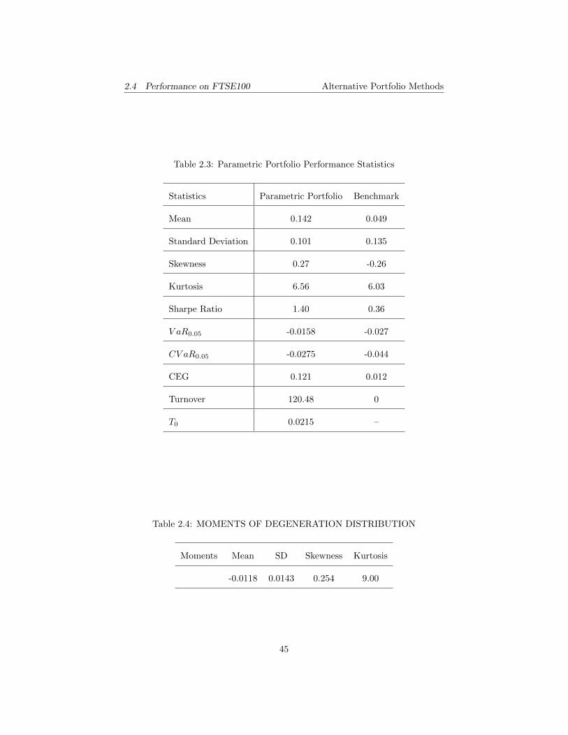
Table 2.3: Parametric Portfolio Performance Statistics
Statistics Parametric Portfolio Benchmark
Mean 0.142 0.049
Standard Deviation 0.101 0.135
Skewness 0.27 -0.26
Kurtosis 6.56 6.03
Sharpe Ratio 1.40 0.36
V aR0.05 -0.0158 -0.027
CV aR0.05 -0.0275 -0.044
CEG 0.121 0.012
Turnover 120.48 0
T0 0.0215 –
Table 2.4: MOMENTS OF DEGENERATION DISTRIBUTION
Moments Mean SD Skewness Kurtosis
-0.0118 0.0143 0.254 9.00
45

2.4 Performance on FTSE100 Alternative Portfolio Methods
Figure 2.2: Rolling Breakeven Transation Cost
These characteristics data are standardized cross-sectionally to subject to stan-
dard normal distribution N(0, 1) before applying to parametric portfolio model.
The standardization brings about several benefits. First, standardization unifies
the scale of all characteristics so that the possibility of overestimating coefficient
effect just because of its larger calibration. Second, the original cross-section
characteristics data may be nonstationary, while the standardized ones are defi-
nitely stationary. Furthermore, standardization makes the total deviations from
benchmark portfolio equal to zero and hence the sum of optimal portfolio weights
to be one.
As for portfolio optimization, the first period of data is used for in-sample es-
timation for initial optimal weights while the second period for out-of-sample
experiment.
Certainty equivalence gain (CEG) in Table (??) is calculated using CRRA func-
tion which indicates investors indifference between a risky gain and its CEG.
46
2.4 Performance on FTSE100 Alternative Portfolio Methods
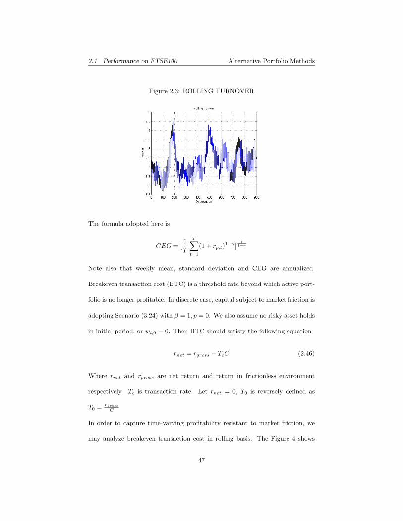
Figure 2.3: ROLLING TURNOVER
The formula adopted here is
CEG = [1
T
T∑t=1
(1 + rp,t)1−γ ]
11−γ
Note also that weekly mean, standard deviation and CEG are annualized.
Breakeven transaction cost (BTC) is a threshold rate beyond which active port-
folio is no longer profitable. In discrete case, capital subject to market friction is
adopting Scenario (3.24) with β = 1, p = 0. We also assume no risky asset holds
in initial period, or wi,0 = 0. Then BTC should satisfy the following equation
rnet = rgross − TcC (2.46)
Where rnet and rgross are net return and return in frictionless environment
respectively. Tc is transaction rate. Let rnet = 0, T0 is reversely defined as
T0 =rgrossC
In order to capture time-varying profitability resistant to market friction, we
may analyze breakeven transaction cost in rolling basis. The Figure 4 shows
47

2.4 Performance on FTSE100 Alternative Portfolio Methods
Figure 2.4: ROLLING CV aR0.05 (WINDOW LENGTH = 100)
Solid line: Parametric Portfolio Dash Line: Equal Weights
the dynamics of BTC with T=52.1
Long-term average breakeven transaction cost is approximately 2% which is
consistent with the statistic on whole sample. But temporary small or even neg-
ative BTC is also present. A check on rolling turnover indicates that variation
of BTC is largely due to instability of return.
It is also possible to calculate risk measure dynamically. Figure 4 compares
rolling CV aR0.05 of equal weights and parametric portfolio.
Overall parametric portfolio has a much better risk profile in most of the time.
Discretion widens in financial crisis when pp profits from persistent down-trend.
And tail risk is effectively managed to be anchored around 0.03 level.
Empirical return distributions are qq-plotted (Figure 5,6,7) to detect existence
1This is the average number of weeks in a year.
48

2.5 Concluding Remarks Alternative Portfolio Methods
of non-nomarlity. Both parametric portfolio and equal weights significantly
deviate from normal distribution. PP offers no help in alleviating ‘fat tail. No-
tice that parametric portfolio return is positively leptokurtic to equal weights
scheme while avoiding introducing more negative extreme events. This prop-
erty can achieve better risk/reward profile because more favorable outcomes are
acquired without additional risks.
Finally, out-of-sample degeneration defined as the difference between realized
return and target return has a negatively-skewed distribution. Moments are
summarized in Table 4
As expected, degeneracy exists in parametric portfolio. Its high kurtosis is prob-
lematic since more extremes are anticipated. It is also evidence of difficulty in
forecasting return.
2.5 Concluding Remarks
In this paper, we systematically discussed parameterization in portfolio opti-
mization. The basic model is split policy into benchmark and add-on term that
is factorized. It can be extended considering trading constraints, market friction,
multi-utility and multi-frequency. Its validity is proved in stochastic settings.
Then in order to mechanically select efficient predictors, we first construct a link
between predictability and profitability so that reality check applies. Finally,
performance on FTSE 100 is well documented to demonstrate robustness of the
method. Its flexibility and rich potential advancement is highly appreciated.
49

2.5 Concluding Remarks Alternative Portfolio Methods
Figure 2.5: QQPLOT: Parametric Portfolio vs Normality
Figure 2.6: QQPLOT: Equal Weights vs Normality
50

2.5 Concluding Remarks Alternative Portfolio Methods
Figure 2.7: QQPLOT: Parametric Portfolio vs Equal Weights
Figure 2.8: Out-of-Sample Degeneracy
51

2.6 Appendix Alternative Portfolio Methods
2.6 Appendix
2.6.1 Technical Indicators
Diverse technical trading indicators have been developed to forecast stock price
so far. Modern automated trading system combines multiple rules to generate
accurate trading signals based on genetic algorithm or an artificial neural net-
work. Here in our model, we only chose the rules with best predictive power
for FTSE 100 constituents from huge universe of technical indicators. Below
is a brief view of trading rules under consideration, prominently featured by
Murphy (1999) and Kaufman (2005).
EMA (exponential moving average rules)
Exponential moving average is a trend following indicator screening fluctuations,
thus identifying major trend of price efficiently. It entails variable weights to
each price according to length of its history. In other words, it assigns heav-
ier weights to data points the more recent they are and the weights decays
exponentially, as is represented by formula (2.47)
Mt(n|Pt) = (1− 2
n+ 1)Mt−1(n) +
2
n+ 1Pt (2.47)
Where Mt denotes EMA value at time t, Pt denotes stock prices, n represents
the length of time periods considered. Common rule of EMA is to generate buy
or sell signal by crossover of a fast (s) and slow (l) EMA line. Or
∆Mt(n1, n2|Pt) = Mt(n1|Pt)−Mt(n2|Pt) (2.48)
52

2.6 Appendix Alternative Portfolio Methods
In order to remove weak and false signals, filters should be added to the rule.
Fixed band (b) that requires crossover big enough to exceed a minimum range
is imposed. In addition, holding period for a given position (h), ignoring any
signals triggered in subsequent periods, should also be considered in the rules.
EMA rules parameters are designed as below:
n1=1, 2, 3, 4, 5, 7, 10 (7 values)
n2=5, 10, 15, 20, 25, 30, 35, 40 (8 values)
b=0.001, 0.005, 0.01, 0.05 (4 values)
h=5, 10, 15, 20 (4 values)
Note that s must be smaller than l.
ROC (rate of change rules)
ROC is the percentage difference between current closing price and the price
several time periods ago. It measures the speed at which price is moving, hence
generating trading signals (See equation (2.49))
Rt(n|Pt) = logPt − logPt−n (2.49)
(2.49), Pt and Pt−n represent stock closing price now and n periods ago respec-
tively. The midpoint of ROC is zero. When it crosses above (below) zero, a
buy (sell) signal is sent out. Sometimes we may filter trading signal by some
smoothers like Parameters of this rule:
Rt(n,L|Pt) = Mt(L|Rt(n;Pt)) (2.50)
n=1, 2, 3, 4, 5, 7, 10, 12 (8 values)
53

2.6 Appendix Alternative Portfolio Methods
RSI (relative strength index rules)
The relative strength index is among famous momentum oscillators, whose value
volatile around a midpoint line and function well in predicting price trend rever-
sals. RSI is defined as the relative value between stock recent gains and losses.
It is calculated as:
St(n|Pt) = 100− 100
1 +RSt(n|Pt)(2.51)
where RS denotes the ratio of average of n periods up closing prices to the
average of n periods down closes. (Murphy, 1999)
Its value fluctuates between 0-100, with 50 as its midpoint. When RSI line
crosses over the upper boundary (100−LR), there is high possibility that prices
fall in the following periods. Conversely, if it breaks below the oversold threshold
(LR), investors can expect a strong rise in price in the future. Parameters
include
n=3, 4, 5, 6, 7, 8, 9, 10, 11, 12, 13, 14 (12 values)
LR=6, 8, 10, 12, 14, 16, 18, 20, 22, 24, 26, 28, 30 (13 values)
Support and Resistance Rules
This system produce buy or sell signals according to whether closing price ex-
ceeds the minimum or maximum level over the past n periods. As with the
moving average rules, fixed band filters (b), and holding period requirements
(h) can be imposed.
Parameters:
n=5, 10, 15, 20, 25, 50 (6 values)
54

2.6 Appendix Alternative Portfolio Methods
h=5, 10, 15, 20 (4 values)
ALR (Alexanders Filter Rules)
Unlike rules above, ALR generate initiating and liquidating position signals.
Investors should initiate a long (short) position when current closing price rises
by x% above (below) its recent extreme low (high), defined as the lowest (high-
est) closing price obtained during a short (long) position trading period, and
liquidate long (short) position held when todays closing price falls (rises) below
recent extreme high (low).
Parameters are set as:
x=0.005, 0.01, 0.015, 0.02, 0.025, 0.03, 0.035, 0.04, 0.045, 0.05 (10 values)
y=0.005, 0.01, 0.015, 0.02, 0.025, 0.03, 0.035, 0.04, 0.045, 0.05, 0.06, 0.08 (12
values)
All the tested technical trading rules from the five systems above add up to
1140.
55

Alternative Portfolio Methods
3 On Investor’s Pessmism
3.1 Background
As Von Neumann and Morgenstern (1944) and Salvage (1954) axiomatized ex-
pected utility under uncertainty, capital allocation among a set of risky assets
becomes a classical decision making problem. Pioneered by Markowitz (1952,
1959), mean-variance framework has been dominant as a standard model in
most textbooks. Just as controversies on expected utility, MV has never been
accepted with irrefutable evidence. Critiques are mainly categorized into two
disadvantages: paradoxical assumptions on preferences or return distribution
(Quiggin (1981, 1993)), and accurate calibration of expected return and covari-
ance matrix (Bawa et al. (1979); Michaud (1989)). Markowitz (2012) opposed
the assertion that neither quadratic utility function nor Gaussian distribution
is required. These conditions are sufficient rather than necessary. There are
subsequently numerous efforts in literature on dealing with the second issue.
Estimating expected mean has been constructively discussed by Jobson and
Korkie (1980), Michaud (1989). Stability of correlations has attracted concerns
as well (like Engle (2002); Bouchaud and Potters (2009); Laloux et al. (2000)).
Black and Litterman (1992) introduced Bayesian method and updating belief in
optimization procedure. Continuous-time mean-variance approach is developed
recently. (Lindberg (2009))
Paralleling to expected utility, Schmeidler (1986); Quiggin (1993), Quiggin (1981)
introduced Choquet utility function for incorporating subjectivity. Artzner et al.
56

3.1 Background Alternative Portfolio Methods
(1999) lay axiomatic foundation for coherent risk measure. Several papers con-
tribute to developing portfolio schemes using VaR and CVaR (Rockafellar and
Uryasev (2000, 2002); Jaschke and Kuchler (2001)). The basic idea is to intro-
duce an objective function with optimal parameters equal to the ones in VaR
and CVaR. The stochastic programming problem can then be discretely solved.
Another significant advancement is proposed by Bassett et al. (2004),Koenker
(2005). Portfolios with a family of regular coherent risk measures are translated
to classical quantile regression which is, however, essentially equivalent to Rock-
afeller approach in alpha-risk case. Despite of economic attractiveness of those
procedures, the Achilles heel is inefficient estimation of tail risk. Since events
are rarely observed in sample, risk of calibration might be severely high due to
sampling variation (Jorison, 1996).
In regards with instability of inputs to optimizers, Brandt et al. (2009) design a
parametric scheme that avoids predicting return and risk via maximizing utility
function directly. It is especially superior with large asset base where estimation
error is exponentially magnified. Following the spirit of parameterization, it is
possible to factorize pessimistic portfolio weights to form parametric pessimistic
portfolio. It inherits both the higher tolerance to data-snooping that most op-
timizers suffer and better flexibility which pessimistic portfolio delivers.
In sum, this paper is focused on discussing extensive framework of pessimistic
investment strategies and empirically comparing the approaches with MV ap-
proach and benchmark using global equity index data. The left part is orga-
nized as: general models starting from utility maximization are developed in
57

3.2 Pessimistic Models Alternative Portfolio Methods
section 2; experiment details are described in data and performance; evaluation
of efficiency is then discussed in quantile characteristics, degeneracy, robust-
ness followed by a bootstrap that potentially alleviates overconcentration and
conclusion.
3.2 Pessimistic Models
3.2.1 Quadratic Utility Function and Coherent Risk Measure
Consider a set of lotteries X = [X1, ..., Xn]′
and weight vector w = [w1, ...wn]′.
A portfolio consisting of them can be expressed as Xp = w′X. Denote F (X)
probability distribution of the random vector X, expected utility of compounded
lottery is
EFu(Xp) =
∫ ∞−∞
u(Xp)dF (X) (3.1)
Using Taylor expansion approximating utility around expectation (Markowitz
2012), which gives
u(Xp) ≈ u(w′EX) +
∂u(w′EX)
∂Xw′(X − EX)− 1
2
∂2u(w′)
(∂X)2w′V w (3.2)
We assume utility function is second-order differentiable. Expectation of lot-
teries and covariance matrix are defined by EX =∫∞−∞XdF (X) and V =
(X−EX)(X−EX)′, respectively. Substitute utility with approximation (3.2),
we attain
EFu(Xp) = u(w′EX)− 1
2
∂2u(w′EX)
w′Σw(3.3)
58

3.2 Pessimistic Models Alternative Portfolio Methods
Σ is the covariance matrix on probability space of F (X). Equation (3.3) trans-
forms maximization of expected utility into quadratic programming problem.
Denote δ = 12∂2u(w
′EX)
w′Σwrisk aversion coefficient, classical mean variance analy-
sis becomes
minwδw′Σw
Given utility level, which is equivalent to a linear constraint w′EX = µ0. Note
that we did not pre-assume either probability distribution of random variables
or quadratic utility function, which is emphasized to verify the validity of mean-
variance framework. Therefore, Markowitz (1959, 2012) argued that Gaussian
distribution and quadratic utility form are sufficient but not necessary condi-
tions. As mentioned earlier, a set of distributions is always compatible with
this approach. But we still need the assertion that expectation of return and
covariance matrix can be reasonably calibrated.
The formulation above relies heavily on the accuracy of the quadratic approxi-
mation. Sometimes ineligible effect from higher order moment may significantly
deteriorate applicability of MV approach.
Back to expected utility, let X = F−1(t), definition (3.1) becomes:
EFu(F−1(t)) =
∫ ∞−∞
u(F−1(t))dt
It shows that expected utility is essentially a uniform integral on R. Alterna-
tively, if distortion function is introduced to capture asymmetry of preference,
we may obtain
59

3.2 Pessimistic Models Alternative Portfolio Methods
EFu(F−1(t)) =
∫ ∞−∞
u(F−1(t))dγ(t) (3.4)
This is expected Choquet utility. Specifically, conditional VaR φα(X) or α−risk
measure under wide investigation, has a capacity of γ(α,X) = minXα , 1. Bas-
sett et al. (2004) proved that a portfolio selection that minimizes the function
of φα(X) − λEX is a quantile regression problem minε∈REρα(X − ε) by the
following theorem.
Theorem 3.1 (Bassett et al. (2004)) If EX <∞, then
minε∈R
Eρα(X − ε) = α(φα(X) + EX) (3.5)
Their work also shows that any pessimistic risk measure, by definition, is a
Choquet integral of α−risk measure for some probability measure:
φ(X) =
∫ ∞−∞
γ(α, x)dϕ(α)
The equivalence between coherence and pessimism makes quantile solution a
tractable paradigm to all coherent risk measure. Despite of its universality, we
will restrict our investigation within α−risk measure in this paper.
3.2.2 Optimization of Conditional Value-at-Risk and Pessimistic Port-
folio
Not surprisingly, optimization of conditional value-at-risk developed by Rock-
afellar and Uryasev (2000) is connected to pessimistic portfolio, since both adopt
60

3.2 Pessimistic Models Alternative Portfolio Methods
α-risk in bi-criteria optimization problem. The former approach, however, first
constructs loss function ρ(z), z ∈ Rn associated with the outcome measured
by loss that could be subsequently discretized and solved as a classical linear
programming optimization. The latter analogously translate the problem in
quantile regression which is essentially employing the same technique. Thus
paralleling two methods is considered as an attempt to setting up a consistent
CVaR optimization procedure.
Start from general expression of ρ(z) with respect to α, η is (Pflug, 2000)
ρα(z, η) = η +1
1− αE[z − η]+ (3.6)
Where expectation takes the form of E[z − η]+ =∫∞η
(z − η)dF (z). To gain
intuitive understanding, a piecewise loss function defined on real-valued random
variables is given as:
Lα = z z > η
η[1− αF (η) ] z ≤ η
Without much algebra, we prove the following proposition
Proposition 3.2
ρα(z, η) =1
1− αELα(z, η)
One remarkable property of ρα(z, η) is the constant penalty rate imposed on loss
lower than threshold level α, albeit linear relation is reserved in upper side. This
asymmetry indicates pessimism consistent with coherent risk measure (Koenker,
2005) and leads to the difference from volatility. Also notice that ρα(z, η) may
not be continuous at X = η. More accurately, outcome below some breakpoint
61

3.2 Pessimistic Models Alternative Portfolio Methods
always delivers no lower satisfaction. And continuity is achieved if and only if
α = 0. Another scenario worth noting is α = 1, loss function ρ(z) is no longer
bounded. ρα(z, η) has abrupt shift but is still finite.
In Choquet utility setting, such proposition applies:
Proposition 3.3 Consider distortion function
γα(X) = max1, Xη
and linear utility
u(X) =1
1− α(X +
η(F (η)− α)
1− F (η))
ρ(z) =∫u(X)dγα(X) is a Choquet utility. It is coherent and pessimistic. Specif-
ically, if F (η) is chosen to be α, ρ(z) degrades to α−risk.
Theorem 3.4 (Rockafellar and Uraysev, 2000) As function of α, ρα(z, η)
is convex and continuously differentiable. CV aRα associated with any z ∈ Rn
is determined by
minη∈R
ρα(z, η) (3.7)
And V aRα is jointly derived by the value of η attaining the minimum
V aRα = arg minη∈R
ρα(z, η) (3.8)
Proof. By expressing expectation with integral, equation (3.6) reads
ρα(z, η) = η +1
1− α
∫ ∞η
zF (z)− η
1− α[1− F (η)]
Taking first-order condition with respect to η, as it is continuously differentiable
−α+ F (η)
1− α= 0
62

3.2 Pessimistic Models Alternative Portfolio Methods
Which gives F (η∗) = α or η∗ = F−1(α). We then plug the η∗ into equation
(3.6) to obtain
ρα(z, η) = F−1 +1
1− α
∫ ∞F−1
[z − F−1(α)]+dF (z)
= F−1 +1
1− αzdF (z)− F−1 =
1
1− αzdF (z)
Doing further expansion
ρα(z, η) =1
1− α
∫ ∞F−1
zdF (z) =1
1− α
∫ ∞−∞
zdF (z)− 1
1− α
∫ F−1
−∞zdF (z)
=1
1− αE(z)− 1
1− α
∫ F−1
−∞zdF (z)
Comparing it with equation (3.4) and let γ(α,X) = minXα , 1 completes proof.
One should notice that Theorem (3.4) does not explicitly assume bounded ex-
pectation of z, which is necessary for existence of minimum. The required
condition has caused fragility in the case of tail distribution that first moment
is not finite.
Most importantly, optimal loss function under Rockafellar?s setting combines
an expectation and risk assessment which is essentially the right side of equation
in Theorem (3.1). Thus we restate the last expansion by borrowing definition
of φα(z).
ρα(z, η∗) =1
1− α[E(z) + φα(z)]
Albeit formulating differently, risk measure and loss function share the same
nature. If we apply ρα(z, η) in the context of asset allocation, optimizing CVaR
is to obtain decision vector that minimize ρα(z, η∗)
minw,η
ρα(X′w, η) = min
w,ηη + E[X
′w − η]+ (3.9)
63

3.2 Pessimistic Models Alternative Portfolio Methods
As CV aR captures expected tail risk, objective function (3.6) incorporates first
order moment. A more general version may consider a stochastic programing
problem
Theorem 3.5 (Krokhmal,2006) Let a mapping φ : χ → R satisfies mono-
tonicity, sub-additivity and positive homogeneity defined by Arzner (1999), and
φ(η) > η for all real η, optima of
ρ(z) = infηη + φ(z − η)
Is coherent.
The contribution of Theorem (3.5) is bridging between a mapping with relaxed
properties and coherent risk measure. Solving high moment coherent risk mea-
sure requires linearization with restrictions on number of observation which is
far beyond our discussion. It is believed that its computational cost might pre-
vent wide application.
Further exploring link between pessimistic portfolio and optimization method
by Rockafellar and Uryasev (2000), we establish such proposition:
Proposition 3.6 w, η that minimize loss function in the form of (3.9) is also
solution to quantile regression problem
minw,η
Eρα(X′w − η) (3.10)
64

3.2 Pessimistic Models Alternative Portfolio Methods
Proof. Expand quantile loss function in continuous case
Eρα(X′w − η) = α
∫ ∞η
(X′w − η)dF (X) + (α− 1)
∫ η
−∞(X′w − η)dF (X)
= (α− 1)
∫ ∞−∞
(X′w − η)dF (X) +
∫ ∞η
(X′w − η)dF (X)
= (α− 1)EX′w + (1− α)η +
∫ ∞η
(X′w − η)dF (X)
Since EX only contributes to optimal value, divided by scalar factor, w∗, η∗
achieve minima simultaneously at
minw,η
Eρα(X′w − η)⇔ min
w,ηη +
1
1− α
∫ ∞η
(X′w − η)dF (X)
Which is exactly the loss function (3.10). In discrete case, quantile regression
applies as follows.
Eρα(X′w − η) = (α− 1)
q∑k=1
X′w +
1
q
q∑k=1
[X′w − η]+ + (1− α)η
in which q periods of observations replace integral except some notational changes.
This is consistent with approximate solution proposed by Rockafellar and Urya-
sev (2000).
To be brief, under both continuous and discrete circumstances, pessimistic port-
folio and optimization of CVaR by Rockafellar share the same risk measure and
structure of solution. The former takes the root from Choquet utility maxi-
mization and can be easily extended to a wide range of regular coherent risk
measures. Its elegant tractability, offering additional convenience in bootstrap
analysis, is favored in this paper.
65

3.2 Pessimistic Models Alternative Portfolio Methods
3.2.3 Parametric Pessimistic Portfolio
We may wish to decompose portfolio policy by a benchmark and deviation
that seeks for excess return. This seperation is popular since ability of over-
performance could be evaluated based on some statistics constructed by the
two components. They include, to name a few, Sharpe ratio, information ratio
and Treynor ratio. Generally, active deviation could be motivated by a set of
characteristics, further linearization yields a parameterized expansion.
w(t) = wb(t) +1
N(t)F′(t)β (3.11)
Where w(t) = (w1, ..., wN )′and wb(t) = (w1,b, ..., wN,b)
′are portfolio and bench-
mark weights, respectively. Denote fi(t) = (fi,1, ..., fi,K)′K-dimensional fac-
tor/characteristics vector of the ith asset at time t, and ψj(t) = (ψ1,j , ..., ψN,j)′
cross-sectional vector of jth factor with dimension N at time t. As a result
F (t) = (f1, ..., fN ) = (ψ1, ..., ψK)′
a K ×N factor matrix and β their loadings
to deviation. Here we allow time varying asset base. The convenience of flexibil-
ity is frequently exploited when constituents of benchmark change. The selected
factors are firm-specific. In other words, common factors are not applicable in
equation (3.11).
Multiplying both sides of equation (3.11) by N × 1 unit vector, we obtain
1′w(t) = 1
′wb(t) + 1
N(t)1′F′(t)β. To faciliate comparison, it is reasonable to
ensure that the portfolio is geared by the same leverage with benchmark, which
gives 1′w(t) = 1
′wb(t) irrespective of factors. Thus we should standardize F (t)
66

3.2 Pessimistic Models Alternative Portfolio Methods
to have zero mean cross-sectionally so that 1′F′(t) = 0. Now if we want to
minimize risk given target return µ. With asset return X = (X1, ..., XN )′, it is,
in the context of pessimistic portfolio
minwφα(X
′w) subject to X
′w = µ (3.12)
Replace w in optimization (3.12) with equation (3.11), objective function be-
comes
minwφα(X
′w) = min
βφα(Xb +
1
N(t)X′F′(t)β) (3.13)
Where Xb is return on benchmark portfolio. The second term is weighted av-
erage of unit factor risk exposure. To see this, let ξj = 〈ψj , X〉 be inner prod-
uct of ψj and r, which is the contribution per unit factor j to return. So
FX = ξ = (ξ1, ..., ξK)′
in equation (3.13) indicates our assertion. It offers an-
other interpretation of the optimization: investors assumes βj amount of factor
j that could offset benchmark downside risk and achieve better risk/reward pro-
file. It also states that only those factors that systematically reduce benchmark
risk should be chosen.
Unlike Brandt (2009), Newton’s method can not be applied to the optimization
problem (3.12), because loss function φα(x) is not everywhere differentiable
(Koenker, 2005). The following proposition is valid in the framework of pes-
simistic portfolio.
Proposition 3.7 For bounded benchmark return EXb < ∞, assume finite ex-
pectation ξ = Eξ < ∞ of ξ = 1N ξ = 1
N FX which is the normalized projections
with expectation. Let excess return γ = µ−EXb Solving parametric pessimistic
67

3.2 Pessimistic Models Alternative Portfolio Methods
portfolio optimization problem
minβφα(Xb+ ξ
′β) subject to EXb+ ξ
′β = µ and 1
′w(t) = 1 (3.14)
is equivalent to constrained quantile regression problem
β∗ = − arg minβ,ν
Eρα(Xb − ξ′β − ν) subject to ξ
′β∗ = −γ (3.15)
Proof. In previous discussion, since we standardize factors cross-sectionally,
constraint 1′w(t) = 1 is always satisfied if benchmark weights 1
′wb(t) = 1.
By Theorem 2.1, we have
α(EXb + ξ′β + φα(Xb + ξ
′β)) = min
νEρα(Xb + ξ
′β − ν) (3.16)
Given target return EXb + ξ′β = µ or ξ
′β∗ = γ, optimizing portfolio (3.14) is
to minimize left side of equation (3.16). The right side formulates solution by
letting β∗ = −β.
Remark. We may restate problem (3.15) as a quantile factor model. If bench-
mark return can be interpreted as linear model of factors, it is possible to
eliminate those effect on tail risk by opposite positioning. Alternatively, sys-
temic risk is factorized and hedged. However, this scheme permits under-hedge
or over-hedge as long as target return can be achieved. The trade-off spirit is
essentially constructing efficient frontier on which each portfolio delivers best
return/α-risk profile.
Practically, plug-in method applies after discretizing objective function (3.15)
β∗ = − arg minβ,ν
T∑t=1
ρα(Xt,b − ξ′
tβ − ν)
68

3.2 Pessimistic Models Alternative Portfolio Methods
In more general settings, we may extend α-risk to all pessimistic risk measures
that are able to be represented by α-risk.
Proposition 3.8 Given the assumptions in proposition (3.7), minimizing any
regular coherent risk measure given target return is a weighted quantile loss
function.
By definition, any risk measure that can be expressed as φ(rp) =∫ 1
0φ(rp)dϕ(α)
is pessimistic. Here ϕ(α) is a probability measure. Accordingly, objective func-
tion of parametric pessimistic portfolio becomes a weighted sum of loss func-
tions.
β∗ = −minβ
∫ 1
0
minνα
1
αEρα(rb − ξ
′β − να)dϕ(α)
where ν is α-specific, but slopes do not change. Bassett et al. (2004) proves
that pessimism is equivalent to regular coherence, which justifies our assertion.
Consider ϕ =∑Ni=1 ciI(αi) to be a mass function. it offers a more explicit form.
β∗ = −minβ,ν
T∑t=1
N∑i=1
πiρα(rt,b − ξ′
tβ − νi)
Where weights πi = ciαi
.
A natural extension is to place some restrictions on weights. They are typically
inequalities of equation (3.11) in the form of
Aw = Awb +1
NAF
′β ∈ T ∗
where A is a p × N matrix with number of restrictions p and T ∗ is an real-
valued set. For instance, long-only portfolio is constructed by letting A = IN a
N ×N identity matrix and T ∗ = RN+ . The additional constraints on β hardly
69

3.2 Pessimistic Models Alternative Portfolio Methods
complicate our optimization since it is a standard inequality constrained quantile
regression: see Koenker and Ng (2005) for interior solution procedure.
If cost is incorporated, a trade-off between risk reduction (or return enhancing)
and transaction cost incurred by rebalancing should be considered. In simple
linear scenario, denote c 1 × N cost rate vector. Here the case that cost of
one security might have effect on that of other assets is excluded, thus c can
be viewed as an uncorrelated cost structure and retains less flexibility than the
correlated one. It is allowed to have time-varying c. Our net return that meets
required return as with α-risk becomes:
Erb + ξ′β − cE|∆wb + ∆F
′β| = µ
where ∆wb = wb(t) − wb(t − 1) is the difference of benchmark and ∆F =
1N(t)F (t) − 1
N(t−1)F (t − 1) the difference of deviation. As cost is risk-free, the
objective function associated with coherent risk measure should remain un-
changed. This problem is also
3.2.4 Efficient Frontier and Maximizing Reward/Risk Ratio
The model discussed does not infer a unique solution. As investors vary in risk
tolerance, optimal risk reward pairs extend the efficient frontier. Just as all fea-
sible portfolios are bounded by efficient frontier in mean-variance settings, we
can characterize pessimistic models by risk-reward profile. The central problem
is what risk measure should be adopted to match expected return. A natural
choice, analogously, is the measure consistent with its min-max problem. Fig-
70

3.2 Pessimistic Models Alternative Portfolio Methods
ure 1 shows how risk increases as higher return is targeted. As anticipated, we
indeed demonstrate a concave frontier and a hump reward/risk ratio.
More generally, maximum drawdown (popular among practitioners), VaR ex-
pected shortfalls and traditional standard deviation are also candidates. Yet
whatever measure is used, trade-off relationship between risk and return is com-
monly expected.
In practice, we have to fix portfolio selection for comparison. A common idea
is to set the same target return µ0. The problem associated with this simple
procedure is that instable performance at different return level usually leads to
contradictory conclusions. Another empirical difficulty is that we always have
to set µ0 < supEXt in order to make the problem feasible.
Alternatively, we may consider optimization without constraints like:
minw
δ(s)
s
Here s = σ(w,X)
w′X. σ(w,X) is risk measure concerned while w
′X is expected
return accordingly.
It can be easily shown that for any w ∈ W , there is a wf whose portfolio
performance is on efficient frontier, such that δ(sf )sf≤ δ(s)
s . Thus practically,
searching on global minimum is restricted within boundary. Lai et al.(2011)
shows that mean-variance optimization, under general setting that mean and
variance are unobserved, is maximizing information ratio. The assertion also
holds when we adopt different risk measures. The following proposition is a
simplified justification of our procedure.
71

3.3 Empirical Study on Global Indices PortfolioAlternative Portfolio Methods
Figure 3.1: The upper panel shows concave efficient frontier of pessimistic portfolio, indi-
cating a finite optima can be attained. Conditional value-at-Risk is chosen to be the risk
measure. The Lower panel exhibits hump shape functional of risk/reward ratio on α-risk.
We construct the figure using weekly indices data across 24 countries. Expected return is
calculated historically without annualizing.
Proposition 3.9 For any concave risk measure ρ : w → R, concave reward
measure γ : w → R, convex decision space χ and bounded constant µ there
exists unique vector w∗ ∈W such that
γ(w∗)− µρ(w∗)
≥ γ(w)− µρ(w)
For all w ∈ χ,w 6= w∗
3.3 Empirical Study on Global Indices Portfolio
3.3.1 Data
We choose major indices of 24 developed economies as representatives to their
stock markets. All weekly price data denominated in local currency are col-
72

3.3 Empirical Study on Global Indices PortfolioAlternative Portfolio Methods
lected from DataStream and logarithmic differenced. Table 1 compiles names
of indices, geographical features and prevailing currencies. Total number of ob-
servations amounts to 624 ranging from 26 January 2001 to 28 December 2012.
In the case that some countries have more than one index available, the one
with highest trading volume is selected. The benefit of the criterion is two-fold.
Liquidity is sufficient for practical implementation of our strategies. A wider
popularity generally indicates enhanced market efficiency which might serve as
a conservatism in our simulation.
Table 3 is summary of descriptive statistics. As observed in return on most finan-
cial instruments, all return distributions are negatively skewed and leptokurtic.
VaR and CVaR vary little across countries, indicating similar historical tail risk.
Only Italy experienced average loss in the sample period.
In order to construct parametric pessimistic portfolio, we choose interest rate,
exchange rate and GDP as three sovereign fundamental inputs, among which
the latter two indicators are log differenced to maintain stationarity. Since these
factors are not weekly observed, we use the value most recently observed for each
round of optimization.
One problem arises from international investment is currency risk hedging be-
cause foreign equity values have to be translated to aggregate performance.
Some empirical evidence has shown convenience of currency hedging in global
asset allocation. (Eun and Resnick, 1988; Perold and Schulman, 1988; Glen
and Jorison 1993). In reality, constructing optimal portfolio cannot neglect the
effect of exchange rate fluctuation. We can employ the techniques developed by
73

3.3 Empirical Study on Global Indices PortfolioAlternative Portfolio Methods
Black (1990), Adler and Prasad (1992), Walker (2008) to partially alleviate, if
not fully eliminate, the risk. Yet our research should not deviate to detailing
implementation issue and concentrate purely on return on speculative capital
gains.
3.3.2 Simulation Results
In order to compare policy efficiency, we conduct simulation with two pessimistic
models (pessimistic portfolio and parametric pessimistic portfolio), mean-variance
approach. At each time t of rebalancing, a segment of sample St up to t with
total number of L observations is collected. It trains optimizers to obtain port-
folio weights w(t). This allocation does not change until rebalancing is again
called. For simplicity, the time interval ∆t is fixed which is the holding period
during which we stick to w(t).
The procedure described may affect performance in two ways. By deliberately
selecting rolling window length, return on certain policy can be boosted. Em-
pirically, it is usually necessary to compromise between the risk of introducing
additional noise and being less adaptive to fresh information which may sig-
nificantly deteriorate efficiency. In our case, in hope of avoiding unintentional
data-snooping, we offer two L for each portfolio. As one generally needs more
data than dimension of assets in pessimistic portfolio and mean-variance ap-
proach, their L1 is much larger than that L2 of parametric pessimistic portfolio.
Another aspect is that policies might behave differently associated with varying
74

3.3 Empirical Study on Global Indices PortfolioAlternative Portfolio Methods
Table 3.1: Details of Indices Data Set
24 indices are selected to construct international equity portfolio, among which 17 are Euro-
pean indices, 2 North American, 4 Asian and 2 Oceanian, respectively, to gain the geographical
diversification. Each indice is a representative of one country equity market. Thus the most
actively traded one is chosen.
Country Main index Region Local Currency
Australia S&P/ASX 200 Oceania Australian Dollar
Austria ATX 200 Europe Euro
Belgium BEL 20 Europe Euro
Canada S&P/TSX North America Canadian Dollar
Denmark OMXC20 Europe Danish Krone
France CAC 40 Europe Euro
Finland OMXH Europe Euro
Germany DAX 30 PERFORMANCE Europe Euro
Greece ATHEX COMPOSITE Europe Euro
Hong Kong HANG SENG Asia Hong Kong Dollar
Ireland ISEQ Europe Euro
Israel ISRAEL TA 100 Asia New Shekel
Italy FTSE MIB Europe Euro
Japan NIKKEI 225 Asia Yen
Netherlands AEX Europe Euro
New Zealand NZX 50 Oceania New Zealand Dollar
Norway OSLO Europe Norwegian Krone
Portugal PSI-20 Europe Euro
Singapore STRAITS TIMES INDEX L Asia Singapore Dollar
Spain IBEX 35 Europe Euro
Sweden OMXS30 Europe Swedish Krona
Switzerland SMI Europe Swiss franc
UK FTSE 100 Europe British Pound
USA S&P 500 North America US Dollar
75

3.3 Empirical Study on Global Indices PortfolioAlternative Portfolio Methods
holding period. To enhance robustness, both weekly and monthly rebalancing
are simulated (∆t = 1 and ∆t = 4 given weekly sampling frequency). Finally,
we also vary significance τ in quantile loss functions, so that sensitivity to tail
risk calibration can be assessed. Our benchmark is allocating equal capital to
each equity index. Table 2 compiles annual return, Sharpe ratio calculated us-
ing annualized return and 2 risk measures both with significance level 0.01.
In all scenarios, active portfolio outperforms benchmark, which indicates ex-
istence of alphas. Parametric portfolio delivers the highest Sharpe ratio irre-
spective to L, τ,∆t. Moreover, its exposure on tail risk is much smaller than
other portfolios, an indication of effective risk control. Despite of mediocre
annual return, it has the best reward/risk profile among all three portfolios.
Mean-variance approach gives the highest return and is especially competitive
alternative in low rebalancing frequency. Pessimistic portfolio overall records
the lowest return and Sharpe ratio. Another feature worth noting is that per-
formance on PPP seems to be insensitive to parameters. Comparatively, return
of mean-variance increases with lower ∆t. This could be caused by mismatch-
ing between in-sample (long-term perspective) and out-of-sample (short-term
fluctuations) return/risk frames.
76

3.3 Empirical Study on Global Indices PortfolioAlternative Portfolio Methods
Table 3.2: Simulation Result From 2001 to 2012
The table shows out-of-sample performance from January 2001 to December 2012 using pes-
simistic portfolio (PP), mean-variance (MV) and parametric pessimistic portfolio (PPP). Each
method applies to a rolling sample to obtain allocation for the next holding period. Simulation
is conducted with two alternative window lengths L. Because one generally needs L N , PP
and MV have L of 150/100 which are much larger than that of PPP (L = 50/25). Loss signif-
icance τ is taken value of 0.1/0.01, to gain difference of pricing tail risk by investors. Portfolio
is rebalanced for each additional observation if holding period is one week. Otherwise, we
allow weights frozen for next one month. Weekly return is annualized to compute Sharpe
ratio, assuming zeros risk-free rate. Tail risk measure, VaR0.01 and CVaR0.01, is calculated
based on empirical distribution of portfolio return.
Rebalance weekly Annual Return Sharpe Ratio VaR0.01 CVaR0.01
L = 100PP
τ = 0.1 0.0206 0.143 -0.0668 -0.0864
τ = 0.01 0.0147 0.091 -0.0756 -0.112
MV – 0.0455 0.240 -0.0730 -0.1235
L = 50 PPPτ = 0.1 0.0327 0.458 -0.0290 -0.0379
τ = 0.01 0.0282 0.396 -0.0290 -0.0379
L = 150PP
τ = 0.1 0.0232 0.191 -0.0635 -0.0950
τ = 0.01 0.0105 0.049 -0.0818 -0.1454
MV – 0.0496 0.245 -0.0812 -0.1373
L = 25 PPPτ = 0.1 0.0387 0.567 -0.0315 -0.0420
τ = 0.01 0.0362 0.537 -0.0315 -0.0394
Rebalance monthly Annual Return Sharpe Ratio VaR0.01 CVaR0.01
L = 100PP
τ = 0.1 0.0184 0.091 -0.0677 -0.1014
τ = 0.01 0.0066 0.036 -0.0782 -0.1219
MV – 0.0672 0.345 -0.0720 -0.1177
L = 50 PPPτ = 0.1 0.0301 0.500 -0.0268 -0.0366
τ = 0.01 0.0289 0.473 -0.0268 -0.0376
L = 150PP
τ = 0.1 0.0127 0.061 -0.0681 -0.1050
τ = 0.01 0.0028 0.007 -0.0758 -0.1365
MV – 0.0615 0.301 -0.0823 -0.1351
L = 25 PPPτ = 0.1 0.0288 0.489 -0.0233 -0.0344
τ = 0.01 0.0277 0.463 -0.0246 -0.0354
Benchmark -0.0049 -0.027 -0.0805 -0.114
77

3.4 Discussion Alternative Portfolio Methods
3.4 Discussion
3.4.1 Tail Distribution Stationarity, Overconcentration and Boot-
strap
The central assumption that justifies minimizing expected adverse tail events
using historical data is stability of tail distribution. Although there is rich
literature discussing the effect of leptokurtic return distributions on portfolio
construction (as early as Mandelbrot, 1963), rarely has any study been con-
ducted on consistency of tail behavior until recently (Straetmans and Cande-
lon, 2013). To capture the dynamics of tail distribution, several researches,
such as Embrechts (1997), Quintos (2001) contribute to designing statistics to
test structural change of extreme returns. Jansen (2000), Danielsson and de
Vries (1997) assess practical constraints placed on portfolio selection. To be
concrete, we introduce rolling α-risk CVaRα to demonstrate its time-varying
characteristics.
In figure 2, CVaRα can persistently deviate from its long-term mean, indicating
?random-walk? nature. Also notice that pessimistic portfolio hardly adapt
to abrupt sizable movement occurring at 2008 financial crisis. It is therefore
showing the fragile nature of extreme negative risk measure.
In multi-variant context, things get worse since concurrence of risk across assets
plays the key role. Similar to covariance matrix in mean-variance approach, joint
risk measure can be remarkably volatile and potentially endanger accuracy of
forecast.
78

3.4 Discussion Alternative Portfolio Methods
Figure 3.2: 100 weeks rolling CVaRα on benchmark return. τ = 0.1
Another problem that partially cohabited with non-stationary tail is caused by
local risk-reward profile. Assets exhibiting superior temporary risk adjusted
return have a strong gravitational effect on capital allocation in the framework
of duality structure (see Section 2). This problem can be remarkably damaging
to pessimistic portfolio. Figure 2 shows an example of such phenomena.
It plots the relation of weights with in-sample target return2. As minimum-
acceptable return level climbs, diversification is diminishing. Extreme case takes
place at the highest achievable target, where only Ireland index is selected. It
ultimately becomes a momentum mechanism.
In figure 6, we offer dynamics of pessimistic portfolio weights with different tar-
get return level. It shows that with higher expected return investor requires,
optimizer tilts to those assets historically performs better. This goes to ex-
treme as the highest return attainable is selected. As Michaud (1989) criticized,
overconcentration has inevitable disadvantages that could lead to poor our-of-
2Return is annualized.L = 100, τ = 0.1
79

3.4 Discussion Alternative Portfolio Methods
sample performance and over-exposure of risk that is presumed to be reduced
through diversification. More risk is assumed due to absence of diversification.
Local behavior dominates resource allocation, incurring additional transaction
cost. Most importantly, it heavily relies on effectiveness of forecasting expected
return using buy-winner strategy, which in most case has lost validity.
In combination with inefficient tail modeling and inappropriate portfolio opti-
mization, resample technique can be employed to properly extract information
from finite sample while retaining stochastic nature of return and risk measure.
We call it bootstrap pessimistic portfolio.
In 1979, Efron first stated bootstrap algorithm, as a generalized resampling
method, to empirically obtain confidence intervals and significance level in the
case of violating normality assumption. Basic algorithm is to randomly select
elements from the distribution of independently, identically distributed observa-
tions to approximate underlying distribution. Some early studies on its asymp-
totical properties and connections with other nonparametric approaches include
Efron (1983), Efron and Tibshirani (1986), Bickel and Freedman (1981), and
Singh (1981).
Some modified bootstrap methods were then proposed to resample from weakly
dependent stationary observations, pioneered by Kunsch (1989) and Liu and
Singh (1992) and later generalized by Politis and Romano (1992a, 1992b) and
Politis, Romano, and Lai (1992). The central idea instead of select single data
point is to conduct ?block resampling?. This philosophy was further improved
by Politis and Romano (1994). It is essentially a weighted average of the block
80

3.4 Discussion Alternative Portfolio Methods
resampling distribution, but the main difference is that the pseudo-time series
obtained by the stationary bootstrap is still stationary and the length of a block
is geometrically distributed. By introducing smoothing parameter q, it is gain-
ing relative stability compared with aforementioned moving block bootstrap.
Recent applications include, not exhaustingly, Boles et al. (2005) and Ledoit
and Wolf (2008).
Our bootstrap pessimistic portfolio essentially consists of two stages:
• Applying stationary bootstrap technique to randomly generate price paths.
• Optimize portfolio on the expanded data set.
The first advantage of this procedure is that diversification benefit is restored.
Consider previous example, bootstrap portfolio no longer overweigh single as-
set3. (Figure 7) And weights vary little with different smoothing parameters. Its
efficiency can be further examined by out-of-sample performance. Let 6 years
up to December 2006 be training set and subsequent 6 years testing period,
performance with or without bootstrap is able to be compared. Significance
level was chosen τ = 0.1.
3.4.2 Quantile Analysis
As it is well known, normal distribution maximizes differential entropy, dictates
that the most probable outcome should follow the distribution whose entropy is
3For simplicity, we average weights on each sample.
81

3.4 Discussion Alternative Portfolio Methods
a local maximum. Thus deviation from normality is an indication of information
loss in portfolio construction, the extent of which might serve as a qualitative
measure of information efficiency.
If two return distribution share the same moment generating function, they
should deliver the same reward/risk ratio. Smirnov (1948) stated that the
supreme of the difference between two distributions should asymptotically con-
verges to the supreme of the absolute value of a Brownian bridge. Thus a
quantile analysis would help identifying distributional consistency. Here, we
use qq plot to illustrate the characteristics. Basically, leptokurtic return bias
left tail downward and right tail upward.
In Figure 2, we construct qq plot for three portfolios and benchmark. As ob-
served, all active schemes fail to control fat tail at both sides. Mean-variance
deviate from the central Gaussian area [µ − εL, µ + εU ] which the others share
similar local feature. To further illustrate relations between two portfolio re-
turns, we plot mean-variance and pessimistic portfolio quantiles over parametric
pessimistic portfolio quantiles. It shows that return on PPP is less leptokurtic,
an evidence of enhancing tail risk control.
3.4.3 Out-of-sample Degeneration
As Davies and Servigny (2012) states, the discretion between realized return and
target return usually exhibits a negatively distorted distribution. The extent
of degeneracy, when extending in-sample allocation scheme beyond, is a critical
part of evaluation. It is also worthy of investigation from the perspective of
82

3.4 Discussion Alternative Portfolio Methods
historical information extraction.
The figure 5 and table 5 show estimation error, which is defined by the difference
between realized return and target return:
et = Wt−1(Xt − EXt−1)
Here denote Wt−1, Xt, EXt−1 portfolio weights at t − 1, asset return at t and
expected asset return at t − 1 respectively. Ideally,Eet = 0 indicates maximal
efficiency that active portfolio can reach. As long as EXt−1 is an unbiased esti-
mator of EXt, et should be symmetric. Thus negative mean indicates inefficient
modeling of return. More severe degeneracy is present in pessimistic portfolio
as both magnitude and uncertainty are higher. One explanation is that tail
distribution can be relatively mobile and instable over time and thus causes
unfavorable misallocation. The phenomenon is well documented by several re-
searchers.
Another aspect we observe is that pessimistic portfolio has remarkable higher-
order advantage in higher order moments (skewness and kurtosis). This is in
connection with risk measure: pessimistic portfolio minimizes tail risk while
mean-variance approach neglects higher order effects in approximation.
3.4.4 Profitability and Resistence to Market Friction
In reality, market friction is hardly negligible but portfolio schemes discussed
previouly are constructed without taking it into consideration. The simplest
measure of resistance to market friction is breakeven transaction cost cb, which
83

3.4 Discussion Alternative Portfolio Methods
is defined as the average return over rebalancing turnover. Table 5 compiles cb
in all simulation scenarios. However under high friction environment, investors
behavior might be distorted to maximize net return. As a result, breakeven
transaction is not an accurate description.
To enhance practicability, we develop a tractable model that is applicable in
high-friction environment. It can be easily extended to any market that is not
immunized from trading cost.
The vector of discrete weights wt at time t satisfies standardization constraint
w′I = 1 which implies that only N − 1 degrees of freedom for the space ∆n
spanned by w.It also indicates zero total increment cross-sectionally∑Ni=1(wt−
wt−1) = 0
Turnover at time t accordingly is defined as the sum of absolute value of differ-
entials:
T (t) =
N∑i=1
|wt − wt−1| (3.17)
This is the capital subject to friction. Denote ci(t) cost rate of asset i at time t
and total cost of complete rebalancing can be expressed as
C(t) =
N∑i=1
ci(t)|wt − wt−1| (3.18)
With respect to Definition (3.18), current literature discussed a revised version
of portfolio optimization by maximizing utility of net portfolio return or max-
imizing net return given upper boundary of risk measure. Deviating from the
integrated procedure, it might be useful to set up generally applicable ?back-
end component?. Basically, the method is to adapt weights derived from some
84

3.4 Discussion Alternative Portfolio Methods
policy to cost, aiming at maximizing net return.
It is advantageous in that original portfolio optimization is not tortured by cost
penalty. It isolates adjustment to friction that is presumably uncorrelated with
investor?s preference.
For simplicity but without losing too much generality, we restrict our discus-
sion on a special case that a proportion β ∈ R1 of capital is rebalanced and
the rest is left untouched. Additionally, we allow a time-varying shrinkage
p = [p1, ..., pN ]′ ∈ RN for each rebalancing. Thus adjusted weights
wt = wt + (1− β)wt−1 − p (3.19)
which become path-dependent. Thus capital subject to friction is
Cβ(t) =
N∑i=1
ci(t)|wi,t − βwi,t−1 − pi| (3.20)
This quantile problem is linked to utility maximization, mean-variance and
mean-variance using VaR and CVaR. Notice that no restrictions are placed
on value of β and α. A negative proportion is valid when portfolio at previous
period is leveraged up. β > 1 is implementable in a way that one essentially
goes short the former policy.
Technical shrinkage pi also has its economic explanation. It may be interpreted
as cash draw periodically from previous base. The total amount reduced is
D(t) = p′1 in each period. At this point, our method has inherited some
constant consumption plan (Merton, 1973) in linear case. We leave stochastic
discount factor over multi-period utility maximization for further research.
To gain some asymptotic properties of wt, some lemmas are introduced.
85

3.4 Discussion Alternative Portfolio Methods
Lemma 3.10 wi = limt→∞Ewi,t exists if Ewi,t = wi and pi are bounded.
Computing some terminal weights at t using the rebalancing policy sequentially
wi,t =
t∑t=1
(1− β)t−s(wi,s − pi) (3.21)
Split wi,s by its expectation and deviation
wi,t =
t∑s=0
(1− β)(t−s)wi +
t∑s=0
(1− β)(t−s)(wi−wi,t)−t∑
s=0
(1− β)(t−s)pi (3.22)
Taking unconditional expectation and let T go to infinity, we have
wi = limt→∞
Ewi,t =1
β(wi − pi) (3.23)
And arrive at Lemma (3.23).
It tells that long-term adjusted weights are proportional to difference between
unadjusted weights and constant cash draw. If no increments is allowed asymp-
totically which is wi = wi, pi = 1−ββ wi It means that when positive capital is
allocated in stock i, partially adjusted portfolio guarantees a positive cash draw.
We may relax individual relation by aggregating (3.23). If overall capitalization
is fixed,∑Ni=1 pi = 1−β
β . The intuition is that positive cash draw is present when
β ∈ (0, 1). It is reasonable because equity change is only associated with capital
inflow and outflow. However this restriction is not placed in this framework or
leverage is also a flexible dimension.
Up to now, it can be summarized as two basic scenarios we are facing. The first
one is to stick to previous weights, whose net portfolio return at t + 1 is given
as
r0p,t+1 =
N∑i=0
wi,t−1ri,t+1 (3.24)
86

3.4 Discussion Alternative Portfolio Methods
The other is the stated partially rebalancing scheme
rβp,t+1 =
N∑i=0
wi,tri,t+1 (3.25)
Thus our portfolio optimization in high friction environment can be interpreted
as maximizing excess return over unbalanced one, which is
maxp,β
E∆rp,t+1 = maxp,β
E[rβp,t+1 − r0p,t+1] (3.26)
Notice that objective function (3.26) does not account for higher moments or
utility profile. It is a simple discretion. It is able to further explore optimization
with some loss function at the sacrifice of tractability. Reality check is also
applicable for robustness.
Proposition 3.11 Assuming fixed time-sequential return on each asset ri,t =
ri and constant transaction cost on each asset ci(t) = ci, (3.26) is a stacked
quantile problem.
Proof. Let us expand (3.25) with (3.19) and (3.20).
rβp,t+1 =
N∑i=0
wi,tri,t+1 =
N∑i=1
ri,t+1(wi,t+(1−β)wi,t−1−pi)−N∑i=1
ci(t+1)|wi,t−βwi,t−1−pi|
So objective function becomes
maxp,β
E∆rp,t+1 = E
N∑i=1
(ri,t+1ψi,t − ci(t)|ψi,t|) (3.27)
Here denote ψi,t = wi,t − βwi,t−1 − pi. Defining τi = − ri2ci
+ 12 , equation (3.26)
is
maxp,β
E∆rp,t+1 = maxp,β
E
N∑i=1
ρτi(ψi,t) (3.28)
87

3.5 Concluding Remarks Alternative Portfolio Methods
rhoτi is quantile loss function. Therefore time-sequential estimation of p, β is
simply solving a stacked quantile regression in the form of
maxp,β
1
T
T∑t=1
N∑i=1
ρτi(ψi,t) (3.29)
Here we allow parameter τ varying cross-sectionally. To ensure its solvability,
τi ∈ (0, 1) indicates that |ri| < ci. This inequality bounds applicability of our
proposal in highly viscous market. Another situation takes place when mag-
nitude of return decreases as frequency increase. For example, daily portfolio
maintenance may suffer more compared to monthly counterpart since daily re-
turn is usually smaller.
Because process (3.19) is truncated by including one period lag, we may char-
acterize this model as quantile AR(1). In the situation that condition |ri| < ci
is violated, it is possible to split equity base with one part suffering higher fric-
tion and the other is free of transaction cost. In the situation that condition
|ri| < ci is violated, it is possible to split equity base with one part suffering
higher friction and the other is free of transaction cost. We plot the dynam-
ics of each portfolio scheme with varying c in figure 8. cb is higher than the
non-adaptive case. Parametric portfolio is much more resistant to friction while
mean-variance approach loses advantage when c > 0.0003.
3.5 Concluding Remarks
In hope of gaining broader acceptance on conservatism on extreme cases, this
paper might be interpreted as an attempt to generalizing pessimism and empir-
88

3.5 Concluding Remarks Alternative Portfolio Methods
ically testing the efficiency among those models. Difficulty in accurate calibra-
tion of risk measures impedes profitable application of pessimistic models. In
the case that tail risk is more volatile than volatility measure, mean-variance
optimization could be more preferred. This phenomenon is documented by our
empirical study in global indices investment.
To avoiding modeling tail distribution of return, we attempt to decompose port-
folio weights and propose a framework of parameterized pessimistic models.
This factorized approach is advantageous in high dimensional asset pool which
most optimizers suffer from. It retains more flexibility in additional constraints
on weights and is less affected by in-sample data-snooping. Overall, the ap-
proach delivers highest risk-adjusted return that is robust to market friction.
As Liu and Cao (2014) suggest, profitability of parametric pessimistic portfolio
is sourced from serial dependence of factors and their explanatory ability on
asset return. Thus a mechanism of assessing factor selection needs further in-
vestigation.
89

3.6 Appendix Alternative Portfolio Methods
3.6 Appendix
3.6.1 Computational aspects of pessimistic models
For pessimistic portfolio with α-risk measure, analogous quantile problem is
given as:
min(β,ξ)∈Rp
n∑i=1
ρα(xi1 −p∑i=2
(xi1 − xij)− ξ) s.t.x′π = µ0 (3.30)
We packaged portfolio coefficients and location parameter in one set under esti-
mation, which is β = (β2, ..., βp, ξ)′. Slack variables u, v convert inequality into
equality constraints.
In order to rearrange it into classical linear programming structure:
minxf′y|Ay = b, y ∈ [γl, γu] (3.31)
γl, γu are lower and upper boundary respectively. And corresponding matrixes
are
y = (u′, v′, β′)′
(3.32)
f = (τe′, (1− τ)e
′, 0)′
(3.33)
b = (x′
1, µ0 − x1)′
(3.34)
Where x1 is the observation vector x1 = (x11, ..., xn1)′. Similarly, observation
matrix is X = (x2, ..., xp). A is an extended matrix, such that target return
constraint is incorporated:
A = (I −I X
O1×n O1×n ∆xj
) (3.35)
90

3.6 Appendix Alternative Portfolio Methods
Here ∆xj is the difference between mean of returns ∆xj = (x2− x1, ..., xp− x1)
Traditionally, the problem is solved by simplex method. It searches optimal
vertex of the polyhedral expanded by constraints, from an initial feasible point.
Usually complexity is increasing as it has more dimensions. In worst cast, Klee-
Minty shows that time consumption goes up exponentially.
Interior point method was considered as the most computationally efficient algo-
rithm for linear programming. Basically, nonlinear terms are added to objective
function. The continuous Lagrangian expression is then differentiated to obtain
first order conditions (known as Karush-Kuhn-Tucker KKT conditions). Affine
scaling step is calculated recursively by Newton method.
For unconstrained quantile regression, Koenker and Portnoy presented primal
and dual functions as
minu,v,bτe
′u+ (1− τ)e
′v|Xb+ u− v = y, (u
′, v′, b′) ∈ R2n ×Rp (3.36)
maxdy′d|X
′d = (1− τ)X
′e, d ∈ [0, 1]n (3.37)
Then Frisch-Newton algorithm can be employed to search for optimal point
following the central path toward boundary.
For quantile regression with linear constraints, primal and dual problems are
similar:
minu,v,bτe
′u+ (1− τ)e
′v|Xb+ u− v = y,Rb ≥ r, (u
′, v′, b′) ∈ R2n ×Rp (3.38)
maxk1,k2y′k1 + r
′k2|X
′k1 +R
′k2 = (1− τ)X
′e, k1 ∈ [0, 1]n, k2 ≥ 0 (3.39)
91

3.6 Appendix Alternative Portfolio Methods
This log-barrier function is formulated to penalize feasible solutions as they
approach the boundary of the constraints set:
L = c′k−y
′(X′k1+R
′k2−b)−w
′(u−k1−s)−u(
∑log k1+
∑log k2+
∑log s)
(3.40)
c is the temporary variable to be estimated, while k = (k′
1, k′
2)′
First order condition provides classical KKT system, which the affine scaling
step is set by Newton?s Method:
dy = (AQ−1A′)−1(r3 +A1Q
−11 r1 +A2Q
−12 r2) (3.41)
dk1 = Q−11 (A
′
1dy − r1) (3.42)
dk2 = Q−12 (A
′
2dy − r2) (3.43)
ds = −dk1 (3.44)
dz = −z −K−1zdk (3.45)
dw = −w − S−1Wdk (3.46)
Q1 = K−11 Z1 + S−1W (3.47)
Q2 = K−12 Z2 (3.48)
Here all notations follow linear programming conventions, with main diagonal
of each matrix the elements of corresponding vectors. As a result, reverse is no
longer costing, and only effort is needed for Cholesky decomposition for the first
equation in iterative algorithm.
This tentative affine scaling step should be further modified, to properly set
92

3.6 Appendix Alternative Portfolio Methods
moving speed toward boundary. The scaling factor is determined by feasibility
checking. If the full affine scaling step is infeasible, Mehrotro predictor-corrector
step should be brought into, which is actually taking ignored bilinear terms into
account. It is essentially anther Newton step starting from previously proposed
point. Formulas are quite similar in this setting:
δy = (AQ−1A′)−1(A1Q
−11 r1 +A2Q
−12 r2) (3.49)
δk1 = Q−11 (A
′
1δy − r1) (3.50)
δk2 = Q−12 (A
′
2δy − r2) (3.51)
δs = −δk1 (3.52)
δz = −z −K−1zδk (3.53)
δw = −w − S−1Wδk (3.54)
r1 = S−1(µe− dSdWe)−K−11 (µe− dK1dZ1e) (3.55)
r2 = −K−12 (µe− dK2dZ2e) (3.56)
Finally, the duality gap is calculated iteratively until it reduces below tolerance
level. The convergence is achieved through trade-off between stickiness to cen-
tral path and gap reducing speed (Gonzago).
Practically, it is difficult for balance, since the process is path-dependent and
fairly sensitive to initial point. Koenker and Pin states that d0 = (1 − τ)e
is a natural initial feasible point for inequality constrained quantile regression.
However the variable z is also flexible and has a significant impact on conver-
gence rate. z2 6= 0 is an additional constraint, yet it can be shown that any
93

3.6 Appendix Alternative Portfolio Methods
value assigned to z2 would significantly deteriorates efficiency of interior point
method.
Therefore, more robust initial point is essential in the algorithm.
94

3.7 Tables and Figures Alternative Portfolio Methods
3.7 Tables and Figures
Table 3.3: Descriptive Statistics of Country Indices
Country Mean SD Skewness Kurtosis VaR0.01 CVaR0.01 VaR0.05 CVaR0.05
Australia 0.00093 0.0204 -0.8476 8.815 -0.0604 -0.0807 -0.0339 -0.0500
Austria 0.00092 0.0327 -1.1861 14.540 -0.0988 -0.1425 -0.0491 -0.0818
Belgium 0.00046 0.0268 -1.1633 12.653 -0.0814 -0.1130 -0.0451 -0.0670
Canada 0.00117 0.0222 -0.9475 10.932 -0.0670 -0.0998 -0.0339 -0.0553
Denmark 0.00128 0.0267 -0.9791 10.214 -0.0712 -0.1152 -0.0407 -0.0641
France 0.00066 0.0299 -0.6744 7.747 -0.0860 -0.1143 -0.0475 -0.0690
Finland 0.00127 0.0372 -0.5399 6.263 -0.1087 -0.1446 -0.0578 -0.0912
Germany 0.00167 0.0303 -0.6586 7.743 -0.0838 -0.1171 -0.0486 -0.0719
Greece 0.00086 0.0421 0.0983 6.370 -0.1256 -0.1526 -0.0656 -0.0958
Hong Kong 0.00214 0.0366 -1.2987 14.752 -0.0975 -0.1575 -0.0541 -0.0857
Ireland 0.00150 0.0295 -1.5688 15.735 -0.0928 -0.1406 -0.0447 -0.0739
Israel 0.00243 0.0360 -0.6029 5.678 -0.1205 -0.1392 -0.0617 -0.0873
Italy -0.0005 0.0348 -0.7602 9.022 -0.1325 -0.1581 -0.0576 -0.0875
Japan 0.00016 0.0285 -0.8494 10.184 -0.0769 -0.1121 -0.0460 -0.0672
Netherlands 0.00125 0.0287 -1.1806 12.248 -0.0959 -0.1255 -0.0451 -0.0721
New Zealand 0.00029 0.0169 -0.8382 7.912 -0.0551 -0.0706 -0.0259 -0.0428
Norway 0.00225 0.0293 -1.0754 10.067 -0.0874 -0.1318 -0.0467 -0.0730
Portugal 0.00060 0.0268 -0.8859 9.995 -0.0917 -0.1209 -0.0416 -0.0650
Singapore 0.00056 0.0286 -0.4028 7.809 -0.0732 -0.1175 -0.0469 -0.0674
Spain 0.00094 0.0315 -0.7408 8.308 -0.0856 -0.1295 -0.0496 -0.0745
Sweden 0.00177 0.0315 -0.4523 7.142 -0.0861 -0.1178 -0.0507 -0.0733
Switzerland 0.00118 0.0259 -0.8744 14.034 -0.0721 -0.1122 -0.0398 -0.0612
UK 0.00125 0.0242 -1.3656 17.338 -0.0633 -0.1004 -0.0351 -0.0565
USA 0.00146 0.0232 -0.8104 9.393 -0.0707 0.0963 -0.0354 -0.0558
95

3.7 Tables and Figures Alternative Portfolio Methods
Table 3.4: Out-of-Sample Performance of Boostrap Pessimistic Portfolio, Jan-
uary 2007 - December 2012
Under real data option, we directly use the sample of first 6 years to train pessimistic portfolio,
which is classical plug-in method. In other scenarios, stationary bootrap method is employed
to compute average weights. q is the smooth parameter.
Quantile Annual Return Sharpe Ratio
Real Data 1 0.0285 0.204
Real Data 10 0.0346 0.205
Real Data 20 -0.0179 -0.070
q = 0.5 1 0.0269 0.203
q = 0.5 10 0.0343 0.205
q = 0.5 20 0.0424 0.222
q = 0.1 1 0.0249 0.191
q = 0.1 10 0.0345 0.207
q = 0.1 20 0.0394 0.209
q = 0.01 1 0.0201 0.150
q = 0.01 10 0.0277 0.163
q = 0.01 20 0.0222 0.112
96

3.7 Tables and Figures Alternative Portfolio Methods
Table 3.5: Out-of-Sample Degeneracy Moments
Each moment is based on difference between realized return and in-sample target return.
Parameters of MV and PP are L1 = 100, τ = 0.1,∆t = 4. PPP1 colume has a rolling window
length L2 = 25 while the last colume L2 = 50.
PP MV PPP1 PPP2
Mean -0.0015 -0.0013 -0.0013 -0.0017
Standard Deviation 0.0218 0.0194 0.0094 0.0089
Skewness -1.190 -1.581 -0.8562 -0.743
Kurtosis 11.68 21.67 7.0996 6.624
97

3.7 Tables and Figures Alternative Portfolio Methods
Table 3.6: Breakeven Transaction Cost
Breakeven transaction cost is ratio between annual return and average turnover, measuring
vulnerability of portfolio profitability to market friction. Parametric pessimistic portfolio has
overall the highest cb due to significant lower turnover. Mean-variance suffers from volatile
capital re-allocation. Thus its return deteriorates with increasing transaction cost.
Rebalance weekly Total Turnover cb
L = 100PP
τ = 0.1 598.99 0.0014
τ = 0.01 556.19 0.0008
MV – 789.70 0.0026
L = 50 PPPτ = 0.1 254.35 0.0068
τ = 0.01 277.66 0.0069
L = 150PP
τ = 0.1 516.91 0.0013
τ = 0.01 511.12 0.0012
MV – 600.30 0.0036
L = 25 PPPτ = 0.1 303.95 0.0059
τ = 0.01 283.53 0.0057
Rebalance monthly Total Turnover b
L = 100PP
τ = 0.1 223.48 0.0025
τ = 0.01 224.89 0.0019
MV – 354.82 0.0046
L = 50 PPPτ = 0.1 207.69 0.010
τ = 0.01 238.38 0.0090
L = 150PP
τ = 0.1 190.91 0.0044
τ = 0.01 211.04 0.0023
MV – 283.51 0.0055
L = 25 PPPτ = 0.1 224.83 0.0099
τ = 0.01 250.85 0.0085
98

3.7 Tables and Figures Alternative Portfolio Methods
(a) Pessimistic Portfolio and Mean Variance
(b) Parametric Pessimistic Portfolio and Benchmark
Figure 3.3: QQ Plot of empirical return distribution vs normal distribution.
As x-axis is quantile of normal distribution, adeviation from the dash fitted line is
evidence of non-normality. Specifically, leptokurtice portfolio returns have downward-
biased left tail and upward-biased right tail. Pessimistic and mean-variance return
are simulated with rolling window length L1 = 100, parametric pessimistic return
L2 = 25. τ = 0.1 in both pessimistic models. All portfolios are rebalanced monthly
(∆t = 4).
99

3.7 Tables and Figures Alternative Portfolio Methods
(a) QQ Plot of MV and PP Return on PPP return
(b) Left Tail and Right Tail
Figure 3.4: QQ Plot Comparison between two simulated returns.
In upper figure, dashed curve shows distributional characteristics between MV and
PPP while solid curve is that of PP. Lower panel plots details at left and right tail.
Parameters: L1 = 100, L2 = 25, τ = 0.1,∆t = 4.
100

3.7 Tables and Figures Alternative Portfolio Methods
(a) PP and MV
(b) PPP with L2 = 25 and L2 = 50
Figure 3.5: Out-of-Sample Degeneracy of three active portfolio schemes.
It is calculated by the difference between training sample target return and realized
return in the holding period. Parameters of upper panel are L1 = 100, τ = 0.1,∆t = 4.
The left figure at lower panel has a rolling window length L2 = 25 while the right one
L2 = 50.
101

3.7 Tables and Figures Alternative Portfolio Methods
Figure 3.6: Portfolio Composition with Various Target Return on December.
2006.
This is an example of pessimistic portfolio weights varying with target return. As µ
increases, allocation tilts to the assets with high in-sample return. τ = 0.1
102

3.7 Tables and Figures Alternative Portfolio Methods
(a) q = 0.5
(b) q = 0.1
(c) q = 0.01
Figure 3.7: Bootstrap Portfolio Composition with Various Target Return on
December. 2006.
Various average resample block lengths q are selected to check stability of bootstrap
pessimistic portfolio. τ = 0.1.103

3.7 Tables and Figures Alternative Portfolio Methods
Figure 3.8: Portfolio profitability resistence to market friction.
Dash line: PP, bold dash line: MV, bold solid line: PPP. Parameters of MV and PP
are L1 = 100, τ = 0.1,∆t = 4. PPP1 colume has a rolling window length L2 = 25
while the last colume L2 = 50.
104

Alternative Portfolio Methods
4 Mean-Variance on Heterogeneous Sample
4.1 Background
The traditional Mean-variance approach has first been investigated by Harry
Markowitz (1952, 1959). Mean-variance model was later carefully researched
and developed to be a framework of strategic asset management (CAPM).
Portfolio optimization is formulated, in this paradigm, as a process of utility
maximization problem by investors (Markowitz, 1956) and analogous optimiz-
ers with constraints such as stochastic dominance by Kuosmann (2004), Giorgi
(2005), Dentcheva (2006) and tail risk by Schmeidler (1989) are invoked. The
spirit of the approach is to minimize risk with given a level of expected re-
turn, based on mean and variance to estimate the diversify risk. Early studies
as early as Markowitz, adopted the expected mean return and standard devi-
ation as the risk of asset to do the asset portfolio. Fisher Black and Robert
Litterman (1992) did the special study for global portfolio optimization. They
used an approach that combines two established tenets of modern portfolio the-
ory, which are the Mean-Variance Model of Markowitz and the Capital Asset
Pricing Model (CPAM) of Sharpe (1964). This approach allows investors to
construct portfolio across global equities, bonds and currencies. Their data set
covered 17 developed countries from January 1975 to August 1991. Through
rolling-window simulation, investors are able to compare ongoing performance
with two strategies: one is investing in the bonds market with high yields, and
the other is in the equities market with high dividend yield relative to bond
105

4.1 Background Alternative Portfolio Methods
yield. Their research could be empirical evidence that investors are indeed in
informational advantage of forming perspective on global portfolio behavior.
Choueifaty and Coignard (2008) find mean-variance portfolio outperforms both
market capitalization weighted portfolio and equity weighted portfolio in long
term investment. And mean-variance portfolio has higher sharp ratio and lower
volatility. Nicholas George Baccash (2010) argues that mean-variance is quite
better for global portfolio. He researches G7, MSCI DM and MSCI EM, find
that emerging markets offer to American investor the best opportunities to reap
the benefits of global equity diversification.
However, mean-variance builds its validity on a set of unrealistic assumptions.
Follmer and Leukert (2000) describe a problem of partial hedging with quadratic
loss function. Actually it is maximizing expected utility with non-negative
marginal utility. Richard (2004) explains why mean-variance optimization is
not useful for investment management. Investors are never perfectly informa-
tionally efficient, and facing the risk of estimating portfolio risk and return
(ambiguity or model uncertainty), and biasedness is unfortunately magnified by
MV optimizers. Michaud (1989) discuss the practical problems of mean-variance
model such as generating suboptimal portfolios far from efficient frontier. Oth-
ers studies also prove that traditional mean-variance could be problematic when
distributional conditions are violated. The main problem of Markowitz model is
that the optimization procedure often results in concentrated portfolios, require-
ment of too much sample data, model lack of robustness and corner solutions.
(see Michaud (1989), Best and Grauer (1991) and Black and Litterman (1992))
106

4.2 Model Configuration Alternative Portfolio Methods
As more critiques focused on unrealistic quadratic utility function assumption,
forecasting error magnifier, some researchers (Engle 2002, Timmermann 2006)
propose several techniques enhancing estimation accuracy in expected return
and covariance matrix. In this chapter, we intend to design a hierarchical
mean-variance portfolio scheme consisting of trading strategy, state classifier
and classical optimizer. The aim is to offering a fresh application of traditional
portfolio technique. The following section is organized as: 3.2 establishes an
explicit mean-variance interpretation both in discrete and continuous case. 3.3
attempts to set up a momentum strategy from path-dependent PDEs. 3.4 in-
troduces data pre-processer as a classifier for various market state. 3.5-3.8 are
an empirical example followed by conclusion.
4.2 Model Configuration
Since risk/reward paradigm has been well established and restated by differ-
ent frameworks, interpretation can be varied from a special case of stochastic
dominance portfolio choice to continuous stochastic multi-period utility maxi-
mization under certain constraints. In this section, we are not so ambitious to
synthesize a comprehensive model applicable to all scenarios, but intending to
demonstrate its error-magnifier nature from econometric perspective.
Consider N risky assets with random returns vector r(t) and a risk free asset
with known return rf (t). Define the excess returns by the difference of the
two, with conditional means and covariance matrix µ(t) and V (t) respectively.
107

4.2 Model Configuration Alternative Portfolio Methods
Assume, for now, that the excess returns i.i.d. with constant moment.
Suppose the investor can only allocate wealth to the N risky securities. In the
absence of a risk-free asset, the mean-variance problem is to choose the vector
of portfolio weights x(t), which represent the investors relative allocations of
wealth to each of the N risky assets, to minimize the variance of the resulting
portfolio return rp(t) = x′r for a predetermined target expected return of the
portfolio rf + µ:
minxV ar(rp) = x′V x (4.1)
Subject to
Erp = x′(rf + µ) and
N∑i=1
xi = 1 (4.2)
The first constraint fixes the expected return of the portfolio to its target and
the second one is a standardized condition to ensure constant leverage in the
risky assets. Applying the Lagrangian and solving the corresponding first-order
conditions, we have the following optimal portfolio weights:
x∗ = Γ + Ψx
With
Γ =1
C4[C2(V −1λ)− C1(V −1λ)] and Ψ =
1
C4[C3(V −1µ)− C1(V −1µ)]
Where λ a scalar factor measuring risk aversion and C1 = λ′V −1µ,C2 =
µ′V −1µ,C3 = λ
′V −1λ,C4 = C2C3 − C2
1 . The minimized portfolio variance
is equal x∗′V x∗.
108

4.2 Model Configuration Alternative Portfolio Methods
The Markowitz paradigm yields two important economic insights. First, it il-
lustrates the effect of diversification. Imperfectly correlated assets can be com-
bined into portfolios with preferred expected return-risk characteristics. Second,
it shows that, once a portfolio is fully diversified, higher expected returns can
only be achieved through more extreme allocations (notice x∗ is linear in µ) and
therefore by taking on more risk. If we have non-zeros risk-free rate, efficient
concave frontier by CAPM is constructed as figure
The problem is also evident as the paradigm relies on accuracy of forecast on ex-
pected return and covariance. To understand mechanism of error magnification,
derivative of optimal weights respect to expected return is given by
dx = αXdt+ σXdW (4.3)
Which has an explicit variance as
V arX(t) = [X(0)]2exp(2αt)[exp(σ2t)− 1]
We define equivalence of two stocks by the same parameter set of α, σ,W in
equation (4.3). Here essentially both characteristics of stochastic process and
driven force of randomness are shared. Path consistency is a strong condition
for stochastic equivalence in this setting. A weak similarity may be defined as
Definition 4.1 Two risky assets are said to be weakly stochastically equivalent
if and only if they shared α, σ.
One interesting aspect concerning the equivalence is that there is no possibility
of arbitrage. Path equivalence guarantees X1 − X2 = 0. Weak equivalence,
109

4.3 Predictability and Trading Strategy DesignAlternative Portfolio Methods
contrarily, indicates non-stationary process of difference that mean-reverting
style strategy does not work. A portfolio P is a positive valued combination of
risky assets which satisfies the following conditions. Consider the identity:
dP
P= w
′ dX
X(4.4)
Where w = w(t) is weight variable vector, reflecting implementing certain port-
folio policy and∑w = 1. X is vector of stock process X1, XN. A passive
portfolio is a portfolio in which the number of shares remains constant which
reads:
dP = v′dX (4.5)
Where v is the fraction of shares in portfolio P . Market portfolio is a passive
portfolio by nave summation of all stocks. A balanced portfolio is a portfolio
of the form (4.4) where all weights w are constant. It has consequently two
parameters αP , σP describing its lognormal process.
With concave utility function, followed by Markowitz (1952, 1956, 1959) and
Merton (1973), CAPM provides efficient portfolios that maximizes investors
utility.
4.3 Predictability and Trading Strategy Design
In this section, we intend to develop a predictor of return from path-dependent
PDEs and time-series momentum, in hope of enhancing mean-variance portfolio
performance.
110

4.3 Predictability and Trading Strategy DesignAlternative Portfolio Methods
Theorem 4.2 (Dupire, B. 2009) Consider the functional running maximum
of the path:
Mt = max0≤µ≤t
Xt(µ)
Here X ∈ Λt ∈ Λ is a path of xt up to time t. xt is a real-valued random
variable with standard Brownian motion dxt = dw. A functional is a mapping
f:Xt → R Then following equation holds:
Mt(u) = mu = x0 +1
2L0u (4.6)
Where u ∈ [0, t] and mu is maximum value at time u. L0u denotes local time
when mu − xu = 0 is satisfied.
Remark: In classical Brownian motion, maximum is proportional to time spent
to beat the maximum. Equation (4.6) however shows momentum effect that
stronger upside potential is associated with the time spent on beating maximum.
It justifies profitability of popular momentum strategy. Note that it doesnt as-
sume fractional Brownian motion which means that even path-standard Brow-
nian motion somewhat exhibit inertia and long-term memory.
We may also define the functional running minimum of the path and obtain the
following results.
Lemma 4.3 Assuming the same condition as Theorem 3.1, consider the func-
tional running minimum of the path:
Kt = f(Xt) = min0≤u≤t
Xt(u)
111

4.3 Predictability and Trading Strategy DesignAlternative Portfolio Methods
Then following equation holds:
Kt(u) = ku = x0 −1
2L0u (4.7)
Lemma 4.4 With conditions and notations the same as Theorem (4.2) and
Lemma (4.3) except dxt = σdw and σ is constant. We have analogous relations:
Mt(u) = mu = x0 +σ
2L0u (4.8)
Kt(u) = ku = x0 −σ
2L0u (4.9)
Remark: (4.8) and (4.9) are consistent with intuition that higher volatility
indicates wider deviation. We may rearrange those equations to demonstrate
relative profit of directional movement:
EDt = (mt − x0)− (x0 − kt) =σ
2(L0
u − L0u)
And define sharpe ratio consequently assuming zeros risk-free rate
srt =Dt
σ=
1
2(L0
u − L0u)
It suggests that contribution of sharpe ratio is the discretion of the time that
price stays at highest level or lowest level.
A profitable strategy thus is designed to gain an exposure on L0u − L0
u. Or
trading signal is generated by sign(L0u−L
0u). To avoid the situation of stagnate
mt or kt when price temporarily moves in adverse direction after a new mt
or kt was achieved, we may allow flexible origin. One practical method is to
fix rolling window length in calculating (L0u,−L
0u), and base decision on most
recent fluctuations.
112

4.4 Nonparametric Classifier Filtering Alternative Portfolio Methods
4.4 Nonparametric Classifier Filtering
4.4.1 K Nearest Neighbors (KNN)
Suppose a real-valued random variable X ∈ Rq and we have a sample of real-
izations X1, , Xn.
In general setting, consider a point in q−dimensional real space X ∈ Rq, and
random variable xi, some distance metric Di = ‖xi −X‖ is defined to measure
similarity. Here xi, i = 1, ...n may be chosen to be feature vector. The or-
der statistics follow definition by Kendall (1956), i.e. Ri =∑nj=1 1(Dj ≤ Di).
The observations that satisfy xi|Ri ≥ k are the k nearest neighbors the most
similar and comparable elements. We therefore are able to construct knn den-
sity estimate and knn regression like kernel method. Note that the classifier
truncates sample to reduce contamination of outliers
Definition 4.5 Suppose X ∈ Rq has multivariate density f(x). A multivariate
uniform kernel to estimate local f(x) at x can be designed inversely proportional
to the rank
f(i) =k
ncR−qi
Where c = πq/2/(Σ((q + 2)/2)) represents space of unit ball expanded in Rq.
Using second-order taylor expansion, it is easy to show that unconditional ex-
pectation of density is true value biased by the square of ranks multiplied by
gradient of f(x). Variance is affected by the expectation of ranks and f(x).
Definition 4.6 Given dependent variable is functionally correlated with ex-
113

4.4 Nonparametric Classifier Filtering Alternative Portfolio Methods
planatory variables:
yi = Ψ(xi) + ei and E(ei|xi) = 0
Simple knn estimator is the arithmetic mean of nearest neighbors:
Ψ(x, k) = E1(Ri ≥ k)yi =1
k
n∑i=1
1(Ri ≥ k)yi
If some weighting function w is introduced, smoothed k-nn estimator is
Ψ(x) =
∑ni=1 w(Ri ≥ k)yi∑ni=1 w(Ri ≥ k)
Cover (1968) first discussed convergence rate for knn algorithm. Short, R. and
Fukanaga, K. (1980,1981) further discussed measures applicable in defining op-
timal distance.
4.4.2 Discriminant Adaptive Nearest Neighbor Classification (DANN)
Nearest neighbor classifier expects a locally constant conditional probability and
spread a sphere to boundarize similar points. This method suffers severely as
dimension increases. It also performs poorly compared to Bayesian technique
when boundaries exhibit distorted nature. Hastie and Tibshirani (1996), De-
lannay, N. et. al. (2006) proposed alternative classification DANN, which is
flexibly adaptable to determine local decision boundaries efficiently. Its proce-
dure is summarized as:
• Set prior metric matrix Γ0 = I (typically identity one) or start from
updated Γi
114

4.5 Data Input and Implementation Alternative Portfolio Methods
• Obtain k nearest neighbors round point concerned xb with some specific
distance measure
• Compute the weighted loss matrics either within the included sample W
or interactive one across two subsets B.
• Conduct bayesian modification by Γi+1 = W−1/2[W 1/2BW−1/2+εI]W 1/2
• Stop iteration until the maximum number of loops is reached, and use the
revised Γ∗
4.5 Data Input and Implementation
Up to now, several blocks have been fragmentally discussed. We are able to
introduce a coherent framework of combining these techniques. The basic idea
is hierarchical structure aiming to maximize portfolio value.
• Use strategies in Section 4.3 as preliminary filter biasing asset return. Pos-
itively skewed distribution tends to enhance absolute overall performance
regardless of portfolio scheme. It offers opportunity to test applicability
of knn mean-variance optimization.
• Cluster similar historical data using knn or DANN. The pre-processing
procedure is acting as a filter purifying local behavior. This is the ma-
jor difference that our approach deviates from traditional mean-variance
analysis.
• c) Apply mean-variance optimizing portfolio.
115

4.5 Data Input and Implementation Alternative Portfolio Methods
Practically indicators characterizing similarity should be defined in advance. In
this research, we focus on a set of technical indicators whose effectiveness can
be properly assessed (White 2000, Timmermann and White 1999). It turns
out that only elements with statistically significant predictive power contribute
positively to purifying samples.
To test efficiency of the approach, we collect 24 global commodity future daily
data including metals, energy, live stocks, agriculture and soft dating back to
1st Jan. 1999. They are traded in Chicago Board of Trade (CBOT), London
Metal Exchange (LME), Inter-Continental Exchange (ICE) and Chicago Metal
Exchange (CME). For each future contract, a joint index that combines the
most actively traded contracts is selected. If one commodity is traded in various
exchanges, only the most liquid contract is chosen. Rolling return is ignored in
this study. Table 4.1 shows contract details and the date of listing. Descriptive
Statistics are summarized in table 4.2.
All commodities during the past 15 years have experienced price appreciation,
reflected by positive mean returns. Ex Ante Volatility is fairly stable cross
section. Unlike stocks, futures differ remarkably in 3rd-order moment, an indi-
cation of diverse directional long-term movement. Applicability of momentum
strategy is anticipated evidenced by much higher kurtosis.
In addition, both V aR0.01 and CV aR0.01 varies significantly relative to V aR0.05
and CV aR0.05, which is more volatile than standard deviation. The phenom-
ena may verify employing mean-variance is preferable to pessimistic portfolio,
116

4.6 Performance Alternative Portfolio Methods
whose performance is heavily influenced by tail risk stationarity. Section 3.4.1
discussed this issue in details.
4.6 Performance
Figure 3.2 plots out-of-sample performance of three portfolio scheme: Mean-
variance approach, nave portfolio that equally invests in each contract and buy-
and-hold benchmark.
Albeit MV approach is able to achieve higher return, the larger volatility can
significantly erod its superiority. Another remarkable advantage is MVs return
is positively skewed, indicating higher proposition of profitable period.
4.7 Analysis
4.7.1 Reality Check on Strategy Profitability
As we discussed in Section 4.5, the revised mean-variance scheme also depends
on effectiveness of trading strategy developed in Section 4.3. Table 4.4 compiles
manipulated return after it is loaded on each contract.
Compared with Table 4.2, mean return shrinks associated with trading strategy.
This is partially because neutral position occupies large portion of trading time
in contrast to full long position in buy-and-long. Standard deviation and tail
risk, on the contrary, is effectively controlled. Skewness and Kurtosis shows its
little improvement in higher order normality. It seems that mixed evaluation
117

4.7 Analysis Alternative Portfolio Methods
results cast doubt on strategy profitability. In order to further investigate its
validity, we adopt reality check proposed by White (2000). Basically it experi-
mentally tests the null hypothesis:
H0 = E[ln(1 + Skr)− ln(1 + S0r)] = 0
Where Sk is trading signal generated by strategy k. r is asset return. S0
represents some benchmark signal. In our case, buy-and-hold serves as basic
policy which means S01. Further details of the technique are referred to Section
6.3. Table 4.5 summarizes p-value with different smooth parameter q, or average
block length of 1/q.
Null hypothesis H0 is fail to reject only in live cattle case. Wheat and cotton
has some mixed conclusion but the trading strategy reserves ability of profiting
in 21 out of 24 contracts. One may note that various smooth parameters provide
consistent p-value which is a major advantage of stationary bootstrap (Romano,
1994)
4.7.2 Robustness
Out-of-sample degeneration is defined by the difference between target return
and realized return. Distribution of mean-variance degeneration is shown in
Figure 4.3.
As Michaud.R (2008) states, active portfolio suffers more or less from the in-
ferior performance relative to training period. It is evoked by inaccuracy in
118

4.8 Concluding Remarks Alternative Portfolio Methods
forecasting techniques or improper modeling of risk pricing as well as data gen-
erating process. Since both asset return and strategy return is leptokurtic, we
may use qq-plot detecting absolute and relative normality
4.8 Concluding Remarks
Mean-variance approach, deserving appraisal mixed with critiques, remains con-
troversial in literature after 60 years debate. Yet however severely it is restricted
by unrealistic assumptions and practical inoperability, dual problem paradigm
or constrained optimization, in the spirit of utility maximization, is still mo-
tivating portfolio research. As the starting point, we attempt to construct a
hierarchical mean-variance to capitalize on directional moment and strategi-
cally allocate resource on state-dependent risk factor. The framework has a
higher profitability than both equal weights scheme and benchmark, but suf-
fers from out-of-sample degeneration and non-normality. It reveals some basic
disadvantages that most active portfolio management cannot avoid.
119

4.9 Appendix Alternative Portfolio Methods
4.9 Appendix
Table 4.1: Contracts Covered in MSCI
Commodity Exchange Category Start Date
Aluminum LME Metal 1st Jan 1999
Copper LME Metal 28th May 2002
Lead LME Metal 1st Jan 1999
Nickel LME Metal 1st Jan 1999
Zinc LME Metal 1st Jan 1999
Gold CME Metal 1st Jan 1999
Silver CME Metal 1st Jan 1999
Light Crude Oil CME Energy 1st Jan 1999
Brent Crude Oil CME Energy 1st Jan 1999
Heating Oil CME Energy 1st Jan 1999
Gasoline CME Energy 20th Oct. 2005
Gas Oil CME Energy 8th Sep. 2003
Natural Gas CME Energy 1st Jan 1999
Lean Hogs CBOT Live Stocks 1st Jan 1999
Live Cattle CBOT Live Stocks 1st Jan 1999
Feeder Cattle CBOT Live Stocks 1st Jan 1999
Wheat CBOT Agriculture 1st Jan 1999
Corn CBOT Agriculture 1st Jan 1999
Soybean CBOT Agriculture 30th Mar. 2006
Coffee CBOT Agriculture 1st Jan 1999
Sugar CBOT Agriculture 1st Jan 1999
Cocoa CBOT Agriculture 1st Jan 1999
Cotton CBOT Agriculture 1st Jan 1999
120
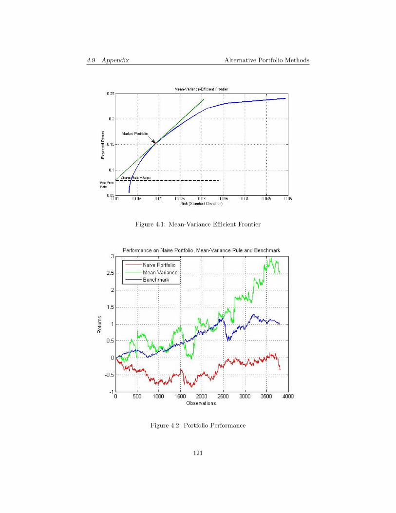
4.9 Appendix Alternative Portfolio Methods
Figure 4.1: Mean-Variance Efficient Frontier
Figure 4.2: Portfolio Performance
121

4.9 Appendix Alternative Portfolio Methods
Figure 4.3: Out-of-Sample Degeneracy
122

4.9 Appendix Alternative Portfolio Methods
(a) Pessimistic Portfolio and Mean Variance
(b) Pessimistic Portfolio and Mean Variance
Figure 4.4: Out-of-Sample Degeneracy
123
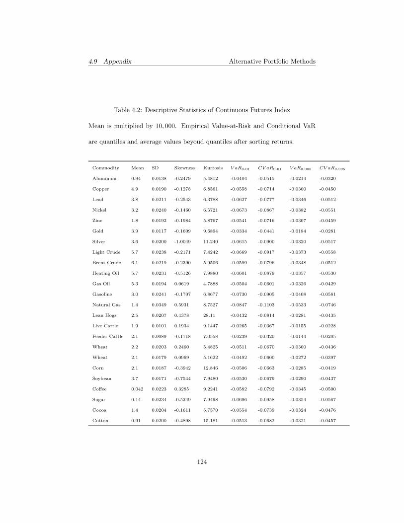
4.9 Appendix Alternative Portfolio Methods
Table 4.2: Descriptive Statistics of Continuous Futures Index
Mean is multiplied by 10, 000. Empirical Value-at-Risk and Conditional VaR
are quantiles and average values beyoud quantiles after sorting returns.
Commodity Mean SD Skewness Kurtosis V aR0.01 CV aR0.01 V aR0.005 CV aR0.005
Aluminum 0.94 0.0138 -0.2479 5.4812 -0.0404 -0.0515 -0.0214 -0.0320
Copper 4.9 0.0190 -0.1278 6.8561 -0.0558 -0.0714 -0.0300 -0.0450
Lead 3.8 0.0211 -0.2543 6.3788 -0.0627 -0.0777 -0.0346 -0.0512
Nickel 3.2 0.0240 -0.1460 6.5721 -0.0673 -0.0867 -0.0382 -0.0551
Zinc 1.8 0.0192 -0.1984 5.8767 -0.0541 -0.0716 -0.0307 -0.0459
Gold 3.9 0.0117 -0.1609 9.6894 -0.0334 -0.0441 -0.0184 -0.0281
Silver 3.6 0.0200 -1.0049 11.240 -0.0615 -0.0900 -0.0320 -0.0517
Light Crude 5.7 0.0238 -0.2171 7.4242 -0.0669 -0.0917 -0.0373 -0.0558
Brent Crude 6.1 0.0219 -0.2390 5.9506 -0.0599 -0.0796 -0.0348 -0.0512
Heating Oil 5.7 0.0231 -0.5126 7.9880 -0.0601 -0.0879 -0.0357 -0.0530
Gas Oil 5.3 0.0194 0.0619 4.7888 -0.0504 -0.0601 -0.0326 -0.0429
Gasoline 3.0 0.0241 -0.1707 6.8677 -0.0730 -0.0905 -0.0408 -0.0581
Natural Gas 1.4 0.0349 0.5931 8.7527 -0.0847 -0.1103 -0.0533 -0.0746
Lean Hogs 2.5 0.0207 0.4378 28.11 -0.0432 -0.0814 -0.0281 -0.0435
Live Cattle 1.9 0.0101 0.1934 9.1447 -0.0265 -0.0367 -0.0155 -0.0228
Feeder Cattle 2.1 0.0089 -0.1718 7.0558 -0.0239 -0.0320 -0.0144 -0.0205
Wheat 2.2 0.0203 0.2460 5.4825 -0.0511 -0.0670 -0.0300 -0.0436
Wheat 2.1 0.0179 0.0969 5.1622 -0.0492 -0.0600 -0.0272 -0.0397
Corn 2.1 0.0187 -0.3942 12.846 -0.0506 -0.0663 -0.0285 -0.0419
Soybean 3.7 0.0171 -0.7544 7.9480 -0.0530 -0.0679 -0.0290 -0.0437
Coffee 0.042 0.0223 0.3285 9.2241 -0.0582 -0.0792 -0.0345 -0.0500
Sugar 0.14 0.0234 -0.5249 7.9498 -0.0696 -0.0958 -0.0354 -0.0567
Cocoa 1.4 0.0204 -0.1611 5.7570 -0.0554 -0.0739 -0.0324 -0.0476
Cotton 0.91 0.0200 -0.4898 15.181 -0.0513 -0.0682 -0.0321 -0.0457
124

4.9 Appendix Alternative Portfolio Methods
Table 4.3: Momentum Strategy Performance
Mean is multiplied by 105 while standard deviation and all tail risk measures
by 104.
Commodity Mean SD Skewness Kurtosis V aR0.01 CV aR0.01 V aR0.005 CV aR0.005
Aluminum 3.8 20 0.2491 33.652 -56 -93 -23 -46
Copper 6.0 25 -0.1971 27.153 -43 -73 -17 -35
Lead 2.6 16 5.0006 171.77 -42 -72 -16 -34
Nickel 4.5 10 0.4184 36.346 -26 -40 -13 -22
Zinc 5.3 17 3.4549 58.328 -50 -69 -18 -36
Gold 5.3 27 -0.3716 53.511 -82 -139 -29 -64
Silver 4.9 16 0.9518 32.878 -49 -77 -19 -39
Light Crude -1.4 11 -0.1709 26.643 -35 -53 -16 -29
Brent Crude 3.5 12 0.1814 18.874 -40 -57 -17 -31
Heating Oil -0.75 11 -0.3096 21.061 -37 -55 -16 -29
Gasoline 1.5 11 0.8728 26.939 -33 -51 -14 -26
Gas Oil 0.22 15 -0.5590 31.879 -48 -76 -20 -38
Natural Gas -0.39 7 -0.6946 23.280 -27 -39 -10 -20
Lean Hogs -3.7 22 -4.8581 171.60 -51 -125 -18 -47
Live Cattle 8.5 26 3.1357 80.278 -71 -115 -26 -56
Feeder Cattle 8.8 26 -0.3764 19.773 -82 -124 -35 -65
Wheat -3.5 12 -3.9207 64.937 -34 -69 -15 -31
Wheat -1.9 14 -1.8019 33.321 -47 -72 -18 -36
Corn -3.7 18 -7.8238 227.23 -54 -99 -20 -44
Soybean 3.6 18 0.8528 23.101 -57 -78 -23 -43
Coffee -2.7 11 0.8992 26.409 -37 -58 -14 -29
Sugar 2.4 13 -2.5954 89.374 -38 -65 -14 -29
Cocoa -2.9 14 -4.9292 150.01 -46 -76 -16 -35
Cotton -3.3 13 -1.2842 60.423 -41 -66 -17 -33
125

4.9 Appendix Alternative Portfolio Methods
Table 4.4: Reality Check p-Value
r is the reality check statistics on return. sr is the reality check statistics on
sharpe ratio.
q = 0.5 q = 0.1 q = 0.02
r sr r sr r sr
Aluminum 0 0 0 0 0 0
Copper 0 0 0 0 0 0
Lead 0 0 0 0 0 0
Nickel 0 0 0 0 0 0
Zinc 0 0 0 0 0 0
Gold 0 0 0 0 0 0
Silver 0 0 0 0 0 0
Light Crude 0 0 0 0 0 0
Brent Crude 0 0 0 0 0 0
Heating Oil 0 0 0 0 0 0
Gasoline 0 0 0 0 0 0
Gas Oil 0 0 0 0 0 0
Natural Gas 0 0 0 0 0 0
Lean Hogs 0 0 0 0 0 0
Live Cattle 1 0.52 0.05 0.06 0.42 0.08
Feeder Cattle 0 0 0 0 0 0
Wheat 0 0.12 0 0.28 0 0.2
Wheat 0 0.02 0 0.04 0 0
Corn 0 0 0 0 0 0
Soybean 3.6 0 0 0 0 0
Coffee 0 0 0 0 0 0
Sugar 0 0 0 0 0 0
Cocoa 0 0 0 0 0 0
Cotton 0 0 0.54 0 0.38 0
126

4.9 Appendix Alternative Portfolio Methods
Table 4.5: Statistics of Performance
Mean and standard deviation are multiplied by 102.
Mean-Variance Naive Benchmark
Mean 16.35 -2.14 6.54
SD 38.48 23.87 14.72
Skewness 1.57 -0.42 -0.32
Kurtosis 41.71 23.73 7.52
Table 4.6: Out-of-Sample Degeneration Moments
Mean and standard deviation are multiplied by 102.
Mean SD Skewness Kurtosis
D -3.7 2.47 1.48 39.95
127

Alternative Portfolio Methods
5 Functional Predictability of Factors and Basis
Portfolios
5.1 Background
5.1.1 Risk Factors
One theoretically critical and practically valuable topic in financial research is
whether and how asset return can be predicted from a set of risk factors. Rich
literature associated with the issue can be roughly categorized by three mo-
tives: exploring new factors that are unexplained by existing ones; measuring
efficiency with alternative statistical approaches; the mechanism that assets are
behaviorally priced. Early attempts to the first dimension might be dated back
to Sharpe (1964) and Black (1972). The failure of well-known CAPM suggests
that cross-sectional return distribution should not be solely dependent on sen-
sitivity to market return. This leads to a generalized version by introducing
more macro indicators (Cox and Ross (1976); Roll and Ross (1980)). Firm-
specific factors, including size (Banz (1981)), leverage effect (Bhandari (1988))
and B/M ratio (also known as HML or B/P ratio) (Chan et al. (1991)) to name
a few, offer interpretation different from unobserved loadings like beta. Their
joint effect on US stocks is then investigated by Fama and French (Fama and
French (1992); Fama and French (1993)). Leverage is abandoned because it is
absorbed by B/M. Endogeneity has to be tackled due to interaction of Beta and
firm size. It is addressed by constructing 100 Size-beta portfolios. In method-
128

5.1 Background Alternative Portfolio Methods
ology session, we will show that there exists an elegant way in the context of
functional dependence.
One effort of subsequent research is disentangling effect of F-F factors and as-
sessing efficiency with new observations. Berk (1995) pointed out that size-
related measure is an evidence of model misspecification rather than a tradi-
tional anomaly. Ali et al. (2001) confirmed that the B/P ratio is a representation
of market mispricing due to high idiosyncratic risk, transaction costs and lower
investor sophistication. Concerning empirical contradiction to F-F result, Pen-
man et al. (2007) found that B/P ratio can be decomposed into enterprise B/M
ratio and leverage component, where the latter, as a proxy of financial distress,
is negatively related to expected return conditioning on B/M ratio. Frazzini
and Pedersen (2014) proposed a tilting strategy of market betas to capitalize
on the compensation for liquidity premium. Apergis and Payne (2014) revisited
size effect in G7 stock markets from 1991 to 2012, using panel threshold cointe-
gration. Their finding is its asymmetric impact after controlling B/M and P/E
ratio.
Another widely-documented anomaly is strong inertia of price movement, pio-
neered by Jegadeesh and Titman (1993). Thay showed that there is persistent
outperformance of buy-winners-sell-losers in US stock market. Carhart (1997)
extended F-F model with momentum factor and generated less pricing error in
contrast with other comparable models. Asness (1997) argued that negative re-
lation between value and momentum is present. Grinblatt and Moskowitz (2004)
studied return dynamics with different time scale and observed that one-year
129

5.1 Background Alternative Portfolio Methods
winners gain but one-month and three-years ones suffer. The research by Shieh
et al. (2012) suggested successful application in NYSE but not AMEX and NAS-
DAQ. Recent advances include the phenomenon that momentum occasionally
crashes during recovery period (Daniel et al. (2012) and Daniel and Moskowitz
(2013)) and remarkable forecastability in residual term in F-M regression (Blitz
et al. (2011)).
Other factors, with continual exploration on behavioral characteristics, are also
burgeoning. Ang et al. (2006) and Ang et al. (2009) reported significant con-
tribution of idiosyncratic volatility. There are also researches on net stock is-
sues effect (Pontiff and Woodgate (2008)) and financial fundamentals, for in-
stance, asset growth effect (Cooper et al. (2008)) and F-score (Piotroski (2000)).
Whether investors require a premium for higher moment risk is investigated by
Kraus and Litzenberger (1976), Amaya et al. (2011). Asness et al. (2013) de-
signed a comprehensive firm quality factor (QMJ) to evaluate firms strength in
four dimensions. Strong profitability of market-neutral strategy on the quality
indicator, which is the average of ranking scores, is empirically evidenced in
US market. However, predictability of QMJ is not statistically supported after
excluding four factors. This inconsistency cast doubt on widely-adopted testing
method.
In regard with growing family of factors and their potential interpretability,
Chen et al. (2010) proposed an alternative three-factor model (CNZ) consisting
of a market risk, an investment factor and ROA. The main intuition is that the
price fluctuation is significantly affected by its discount rate, of which invest-
130

5.1 Background Alternative Portfolio Methods
ment factor and ROA can be good proxies. The empirical results document
an enhancement in U.S. stock market compared to F-F model. Ammann et al.
(2012) applied CNZ in 10 EU countries with data ranging from 1990 to 2006.
They report comparable, if not better, performance.
To summarize, risk factors have three sources: the sensitivity of individual stock
with market index, fundamental elements as indicators of firm′s prospect, and
past performance. The efficiency is from investor behavior and affected by their
perceptions of those risks. Thus as long as factors are fully priced, excess return
is merely a reward for excessive risk exposure.
5.1.2 Empirical Studies on Emerging Stock Market
Due to different regulations, cultures, matching mechanisms, data availability
and investor behavior, emerging markets may vary in risk structure, on which
the researches may offer a test of factors′ universality. In this section, we will
apply cross-sectional analysis for US and Chinese market, in hope of gaining
robustness from comparison.
Claessens et al. (1995), Fama and French (1998) conducted nascent investiga-
tions with the International Finance Cooperation data from 19 and 13 emerging
stock markets, respectively. In spite of slight difference in data sample, they
concluded opposite impacts on market risk, size and value factors. The contra-
diction may be attributed by the difference in modeling technique. More recent
research by Cakici et al. (2013) is examination on momentum and value effect
131

5.1 Background Alternative Portfolio Methods
in 18 emerging market from 1990 to 2011. Price correction for low P/B ratio
is widely documented but buy-winners-sell-losers did not succeed in Eastern
EU. In global context, domestic factors have higher significant interpretability.
Lischewski and Voronkova (2012) investigated existence of liquidity premium
in Warsaw Stock Exchange. The failure of its significant contribution may be
caused by the fact that a large proportion of shares is controlled by a small num-
ber of institutions and compensation of illiquidity is not effectively reflected. On
the contrary, Narayan and Zheng (2010) showed that the risk is priced in Chi-
nese stock market between 1993 and 2003.
In case for Chinese market, size and B/M are considered important, while in-
significance of market beta is caused by individual investors’ irrational behav-
ior and government intervention (Eun and Huang (2007); Wang and Di Iorio
(2007)). With respect to momentum, Naughton et al. (2008) examined alter-
native trading strategies exploiting the anomaly in Shanghai Stock Exchange,
whose profitability explains short-term dynamics in this market. Consistent
with Ang et al. (2006) and Ang et al. (2009), idiosyncratic volatility factor also
has remarkable influence (Eun and Huang (2007); Nartea et al. (2013)).
Our research on emerging market has two-fold benefit. It offers data set of a
counterpart with different legitimate system and market structure, therefore, a
way of ′robustification′. A further study in global market is also rewarded.
132

5.1 Background Alternative Portfolio Methods
5.1.3 Functional Data Analysis
Since stocks exhibit similar behavior cross-sectionally, estimated standard error
would be correlated when applying pooled OLS. One approach, proposed by
Fama and MacBeth (1973), is first to conduct time-series analysis in a rolling
sample and run cross-sectional OLS on de-correlated cross-sectional data. It im-
plicitly assumes linearity of prediction, which is not necessarily satisfied (Hiem-
stra and Jones (1994); Qi and Maddala (1999)). One attempt to tackling non-
linearity is neural network, which typically has several hidden layers trained
to forecast multi outputs via a set of factors (Nicholas Refenes et al. (1994)).
But this method fails to deliver a measure of predictability, therefore, can be
easily contaminated by irrelevant variables. Worse still, it suffers over-fitting in
training sample as information to noise ratio is low. A flexible approach that
is able to offer statistical inference as well as modeling nonlinear dependence is
needed. Another concern of F-M is the difficulty in implementation accounting
for missing observations. This problem is especially severe in emerging markets.
Finally, multivariate analysis is computationally costing accounting for large
data set.
With regard to inefficiencies of current methods, we propose a FDA framework
for testing factor predictability. It is advantageous in dimension reduction. For
example, NYSE has more than 3,600 stocks; similar case is in Chinese A share
market with approximately 2,600 stocks. In this case, idea of continuous curve,
rather than vectors in multivariate analysis, is more appropriate for a large
133

5.1 Background Alternative Portfolio Methods
system. The technique commonly used in smoothing (reducing dimension) is
functional principle component analysis (FPCA), which extracts a set of basis
function that maximally explains variation of the curves (Ramsay and Silver-
man (2005)). By projecting functional objects on orthonormal basis, we are
able to represent them as a vector of scores, where classical analysis applies.
Kokoszka and Reimherr (2013) proved that dependence of the sign of scores is
asymptotically normal and report insignificant simulation results in predicting
intraday shapes of curve. Hyndman and Ullah (2007) proposed a two-step al-
gorithm followed by the principle of FPCA to predict mortality and fertility
rates in France and Australia. Other applications have been further discussed
in many aspects (Ramsay and Silverman (2005);Horvath and Kokoszka (2012);
Mestekemper et al. (2010)).
One successful application of functional forecasting is in vehicle insurance pric-
ing Segovia-Gonzalez et al. (2009). They argued that even though two methods
have the same objective in re-building an entire process within sampling from
different time period, multivariate analysis still bears shortcomings, such as
the difficulty in interpretation of variance-covariance and correlation structure;
while, FDA has its merit in de-noising observations through local information.
Cai and Hall (2006) showed the existence of functional forecasting method, as
well as the difference in properties of functional regression estimation with pre-
diction from an estimator of functional slopes. Sood et al. (2009) reported that a
better prediction of penetration of new products in using augmented functional
model than that of traditional forecasting model. Goia et al. (2010) collected
134

5.1 Background Alternative Portfolio Methods
heating demand curves to forecast intra-daily electricity loading demand. As
samples in the same group exhibit clustered variance but differs massively from
other groups, classification of observations is recommended. The spirit of the
procedure is to enhance prediction accuracy via categorization. Antoch et al.
(2010) argued that electricity consumption are intrinsically different in two pe-
riods, thus grouping objects by weekdays and weekends is valid. A functional
clustering forecast model was proposed by Abraham et al. (2003). James and
Hastie (2001) constructed a functional linear discriminate analysis to classify
new curves.
Asymptotics associated with PCA is dated back to Anderson (1963). Assuming
observations are from a multivariate normal distribution, the function of eigen-
values is asymptotically normally distributed. Hall and Hosseini-Nasab (2006)
showed that the efficiency of eigenvalues in FPCA is dominantly affected by their
spacings. Bootstrap is recommended for constructing confidence interval. Yao
et al. (2005) proposed a method of functional linear analysis whose estimator is
consistent and asymptotically normal. Mas (2007) discussed the conditions of
weak convergence in functional autoregressive model.
At the best of our knowledge, there are few researches employing FDA to analyze
factorized return. One close study by Zhang (2011) is to estimate market beta in
functional CAPM. It differs from our aim, however, in that intraday return curve
is used instead of constructing a functional object of cross-sectional returns. The
difficulty in the latter application is absence of natural topological structure of
a market. Our methodology part is then responsible for designing an algorithm
135

5.2 Methodology Alternative Portfolio Methods
of functionalizing cross-sectional observations.
5.2 Methodology
5.2.1 Inference for functional linear dependence
The primary concern of this part is to design a robust estimator and make
inference on cross-sectional correlation between stock return r = (r1, · · · , rN )T
and factor f = (f1, · · · , fN )T . For simplicity, it is assumed that both r and f are
symmetrically distributed and standardized with zero mean and unit standard
deviation. The null hypothesis is
H0 : ρ =Eπ(r)Tπ(f)
N= 0 (5.1)
Where π is some kennel function reserving monotonicity. It can take either
simple linear form or nonlinear ones that incorporate local information and are
robust to outliers (Devlin et al. (1975)). One common version of the former is
the sample correlation coefficient:
ρc =rT f
N(5.2)
Which is proved to the maximum likelihood estimator under normal distribu-
tion. However, it loses efficiency in case that normality is violated and leads
to contaminated estimation of correlation. One can penalize observations with
large deviations from the mean (Pitas and Venetsanopoulos (1990)) or even trim
tails by introducing Huber bounded function H(z, k) = max−k,min(z, k).
Other two popular methods are based on rank statistics. One is Spearman rank
136

5.2 Methodology Alternative Portfolio Methods
correlation (Spearman (1904)) coefficient
ρc = 1−6∑i=1N (R(ri)−R(fi))
2
N3 −N(5.3)
For a set of observations xi, i = 1, · · · , N, rank operator is,
R(xi) =
N∑j=1
1(xj ≤ xi) (5.4)
where 1 is the identity function. Another is Kendall coefficient τ (Kendall
and Gibbons (1990)), serving as a measure of concordance. Where sgn is sign
function. Asymptotics of them can refer to Kendall and Gibbons (1990), Hjek
et al. (1967).
In the context of forecasting, the interest is whether the effect of lagged factors
on current returns is significant, which has important implication for efficiency of
the predictors. It is easy to show that any market-neutral4 portfolio w, perfectly
concordant with the ranks of factors, delivers positive expected return.
xi, i = 1, · · · , N ifH0 is rejected and τ(w, f) = 1 (5.5)
The intuition is that market anomalies with predictability can always be ex-
ploited by a family of allocation schemes different from nave strategy (equal
weights). But assertion of the inverse relation is not necessarily true. Even if a
profitable portfolio, with functional w(f) is present, predictability of f cannot
be assured.
41Tw = 0
137

5.2 Methodology Alternative Portfolio Methods
The correlation measures discussed previously implicitly require that the num-
ber of stocks equal to that of factors. This assumption may not hold when all
stocks in a market are accounted for, due to frequent listing and delisting. This
problem also exists in the scenario that only constituents of an index are inves-
tigated. The index is rebalanced frequently to maintain its representativeness,
but this additional adjustment exaggerates difficulty in correlation estimation.
Generally speaking, because traditional methods require homogeneous data gen-
erating process, they suffer from a highly changing sample.
Another disadvantage is the poor performance with time-varying correlation.
Consider a modified gross error model Tukey (1960) in which the joint distri-
bution of (rt, ft)at time t conditioning on an unobserved process ρt is given
by
ψ(rt, ft|ρt) = N(rt, ft; 0, 1 + k1(ρt > 0), ρt) (5.6)
Here let k 1. The probability density function is a bivariate normal distri-
bution with zeros mean, asymmetric volatility 1 + k(1ρt > 0) and correlation
structure ρt. We also assume ρt = −ρt−1 so that rt and ft behave exactly the
opposite from the previous period. It is clear to verify thatH0 cannot be rejected
for any of the traditional measures, albeit an evolution of ρt is indeed present.
In consideration of two problems, we propose a functional method aiming at
testing existence of dependence and filtering the path of ρt simultaneously. The
procedure for univariate case is simple.
U.1 Locate stocks in descendent/ascendant order based on their fac-
138

5.2 Methodology Alternative Portfolio Methods
tors and form a cross-sectional return accordingly.
The purpose of the step is to construct a return series that is functionalizable.
In the next section, we will show an alternative that uses time-serial correlation.
As long as a stock has an observation of factor, it always has an unambiguous
location. It can even go delisted when return is no longer available because
smoothing fills the missing data with local information (Ramsay and Silverman
(2005)). One remarkable feature is that stocks are not geographically static
but dependent on the value of factor. If price behaves similarly with specific
rankings, this sorting algorithm offers best arrangement of data.
U.2 Apply functional principle component analysis (FPCA) to the
smoothed return curve and obtain all basis functions Ψ = ψi|E(ξi) 6=
0. Null hypothesis of functional linear test
H0 : Ψ = Ø (5.7)
Specifically, define trend functions Ψ0 = ψ0| |τ(ψ0, f)| = 1. Null hy-
pothesis of linear functional dependence test:
H0′ : E(ξ0) = 0 (5.8)
Because of orthonomality of basis functions, there are only two trend compo-
nents with difference up to sign. By definition, they are in either perfect con-
cordance or complete disorder. Rejection of null is equivalent to assert Ψ0 ⊆ Ψ.
It is obvious that expected score is not zero even in case of gross error model
139

5.2 Methodology Alternative Portfolio Methods
since both scenarios give positive contributions.
The advantages of this procedure are two folds. It extracts continuous (nth
order differentiable) relations with a set of pre-specified continuous functions,
thus retains higher persistence to cross-sectional noise. Moreover, the time
series of scores can be utilized for forecasting predictability of factors. This
topic will be covered in section 5.5. As for multi factor model, the strategy
needs additional dimension reduction.
M.1 Use PCA to find a set of linear combinations f1, · · · , fK of those
factors that accounts for most variation.
M.2 Employ univariate analysis for each principal component f i.
Since f1, · · · , fK are orthogonal, inference in step U.2 for f i is not affected
by other factors. It avoids infeasible multivariate test that has to design sorting
algorithm for all factors. Its additional elegance is the capability of processing
large set of factors exhibiting highly correlated structure.
5.2.2 Functional dependence forecast model
As discussed in 5.2.1, cross-sectional return curve has at least one significant
component. After applying FPCA, PC1 = ψ1; PC2 = ψ2; PC3 = ψ3. As long
as functional linear dependence test implies that expected values of components
ψ∗i deviate from zero (Equation (5.7)), we assert that it has predictability for
140

5.2 Methodology Alternative Portfolio Methods
return at next period in the form of
r(t+ 1) =
K∑i=1
ξi,t+1ψ∗i (t+ 1) (5.9)
However, the above equation is not feasible unless estimates of scores ξi,t+1 can
be attained. Dependence of scores can be weakly tested by adopting Kokoszka
and Reimherr (2013) procedure. The limiting distribution of signs is normal
with null hypothesis:
H0 : Λ(k) = (N − 1)12
N−1∑i−1
I(k)N,nI
kN,n+1
d→ N(0, 1) (5.10)
where I(k)N,n = sign(ξ). Positive (negative) curve shape persistence is anticipated
if H0 is rejected in right (left) tail. Assuming scores follow AR(L) process, which
reads
ξi,t+1 =
L∑j=0
γiξi,t−j (5.11)
Then, equation (5.9) can be estimated as,
r(t+ 1) =
K∑i=1
ξi,t+1ψ∗i (t+ 1) (5.12)
Nevertheless, it is still necessary to prove the r(t+ 1) is an unbiased estimator
of r(t+ 1). In Hilbert space H, we know that r(t) =∑∞i 〈rt, ψi〉ψi(t), where the
operator 〈〉 is the inner product so that 〈rt, ψi〉 is the projection of rt and ψi,
i.e. score of basis function i at time t. Then, we have 〈rt, ψi〉 =∫ 1
0r(t)ψi(t) · dt,
for t ∈ [0, 1]. Note that because r(t) is observed discretely in the real world,
141

5.2 Methodology Alternative Portfolio Methods
〈rt, ψi〉 may be approximated as,
〈rt, ψi〉 =
∫ 1
0
r(t)ψi(t) · dt
≈K∑j=1
1
tj − tj−1· 1
2· (x(tj)ψi(tj) + x(tj−1ψi(tj−1))
(5.13)
Which is simply inner product of two vectors. Now assuming rt is a stationary
functional process, functional curve r(t+1) can be written as following,
r(t+ 1) =
∞∑i=1
〈rt+1, ψi〉ψi(t+ 1) (5.14)
If finite number of basis is sufficient for explaining it (where FPCA applies) with
expected residual vanishing, rearranging equation (5.14) leads to
r(t+ 1) =
K∑i=1
〈rt+1, ψi〉ψi +
∞∑i=K+1
〈rt+1, ψi〉ψi
= r(t+ 1) + ε(t+ 1)
(5.15)
where E(εt) = 0. We can have the expression below from Equation (5.12),
r(t+ 1) =
K∑i=1
ξi,t+1ψi(t+ 1)
=
K∑i=1
L∑j=0
βjξi,t−jψi(t+ 1)
=
K∑i=1
(
L∑j=0
βj〈rt−j , ψi〉)ψi(t+ 1)
(5.16)
The difference between equation (5.15) and equation (5.12) is given by,
r(t+ 1)− r(t+ 1) = r(t+ 1) + εt − r(t+ 1)
=
K∑i=1
〈rt+1, ψi〉ψi −K∑i=1
(
L∑j=0
βj〈rt−j , ψi〉)ψi + εt
=
k∑i=1
[〈rt+1, ψi〉 −L∑j=0
βj〈rt−j , ψi〉]ψi + εt
(5.17)
142

5.2 Methodology Alternative Portfolio Methods
Thus, it is required that the condition below should be satisfied for all i,
〈rt+1, ψi〉 =
L∑j=0
βj〈rt−j , ψi〉 (5.18)
Note that the equation (5.11) merely demonstrates linear relation without basis
functions. Therefore, the estimator rt+1 will be an unbiased estimator for rt+1,
which means any unbiased time-serial estimator of score is valid.
5.2.3 Constructing Portfolio with Basis Functions
A portfolio policy allocates capital across return object aiming at gaining pos-
itive overall performance, thus return on a policy rpt is essentially the inner
product of portfolio weights w(t) and cross-sectional return r(t).
rpt = 〈w(t), r(t)〉 (5.19)
Practically, investment decision is made before return is realized. Following
expansion (5.15)
rpt = 〈w(t), µt +
K∑i=1
ξiψi + ε(t)〉 (5.20)
Randomness is stem from the risk of contributions from each basis function.
Thus functional principal component analysis is regarded as a calibration of
pattern uncertainty. The error term ε(t) has zero correlation with basis function
i.e. E〈ψi, ε(t)〉 = 0.
One should notice that there exists calibration error as ε(t) is not determinstic.
By standard context of functional PCA, it assumes that
V ar(〈ψi, rt〉) = λi (5.21)
143

5.2 Methodology Alternative Portfolio Methods
Consider static basis portfolio linear with some basis function, which is
wi = kψi = sign(E〈ψi, µt〉)ψ (5.22)
If∫ψids = 0, it ensures that our portfolio is a market-neutral strategy . By
letting rt = µt +∑Kj=1〈rt, ψj〉ψj + ε(t) and µt 6= 0, its expected return is
Erit = E〈kψi, µt +
K∑j=1
ξiψj + ε(t)〉
= k(E〈ψi, µt〉+ E
K∑j=1
〈ψi, ξiψj〉+ E〈ψi, ε(t)〉)
= k(E〈ψi, µt〉+ Eξi)
= kE〈ψi, µt〉 = |E〈ψi, µt〉|
(5.23)
Here we use a general assumption that expected score is zero. We now know
that the porfolio with respect to some basis function delivers strictly positve
return as long as it is not orthogonal to the functional mean.
So it is correct that portfolio performance can be boosted if some estimator on
the sign of score can be designed. Further more, the risk associated with it is
V ar(rit) = V ar(〈kψi, ri〉) = λi (5.24)
And Sharpe ratio should be
SRi =(θi − γ)
λi(5.25)
where θi is projection of basis function on functional mean and γ is risk-free
ratio. Equation (5.25) tells that one threshold the score needs exceeding to
guarantee positive Sharpe ratio is γ. It is also affected by the covariance struc-
ture of basis fucntion and the noise remaining unexplained. If those return
144

5.2 Methodology Alternative Portfolio Methods
curves are not independent, it allows an unbiased estimator ξi and cofficient
kt = sign(E〈ψi, µt〉) + ξt, equation (5.23) becomes
Erit = (Ekt〈ψi, µt〉+ Ektξi) = |E〈ψi, µt〉|+ Eξ2i > Erit (5.26)
One may concern a mixed approaches consisted of basis portfolios. By equa-
tion (5.23), excess return Erbt = (|E〈ψ1, µt〉|, ..., |E〈ψK , µt〉|)′ − γ1. Without
losing generality, we assume ki = sign(|E〈ψi, µt〉|) = 1. Since E〈ψi, µt〉 doesn’t
contribute to variability of return curve, covariance structure is
Cb = (rbt − Erbt )′(rbt − Erbt ) = Eξ
′ξ = Cξ (5.27)
Where ξ = (ξ1, ..., ξK)′
is score vector. It is thus clear that two basis portfolios
are intercorrelated with scores. In the framework of mean-variance optimization,
consider maximizing a linear utility function with loss aversion χ and weights
β,
L = β′Erbt − χβ′Cbβ (5.28)
First-order differential with repect to β gives
β =1
χC−1b Erbt (5.29)
When building up a fractional Kelly system on the set of basis portfolios, the
above equation can also be derived with χ the proportion invested in Kelly
portfolio. It degenerates to time-series momentum in case of zeros correlations
among all return series. To obtain (5.29), We may express equity dynamics
of basis portfolio using stochastic process drive by M wiener processes W =
145

5.3 Experiment Alternative Portfolio Methods
(W1, ...,WM )′, then exhibit
dStSt
= θdt+ ΠdW (5.30)
Where St = (S1,t, ..., S′K,t) is equity vector of K basis portfolios at time t. θ
is drift vector defined in equation (5.25) which has the same dimension of K.
Π is a K ×M matrix, capturing the effect of different sources of uncertainty.
considering a portfolio policy by investing β in the risky asset pool and left for
earning risk-free rate γ, equity of our portfolio thus follows the SDE
dAtAt
= (1− β′1)γdt+ β′(θdt+ ΠdW )
= (γ − β′1γ + β′θ)dt+ β′ΠdW
(5.31)
Apply Ito formula and it is easy to see that K×K covariance matrix Π′Π = Cξ
dlog(At) = (γ − β′1γ + β′θ − 1
2β′Cξβ)dt+ β′ΠdW (5.32)
The spirit of Kelly system is then maximizing the drift term, whose first order
condition offers (5.29)
∂D
∂β= −γ1 + θ − Cξβ = Erbt − Cξβ = 0 (5.33)
5.3 Experiment
5.3.1 Implementation Procedure
To apply the method of functional data, we conduct an experiment on the
predictability of momentum effect on return in Chinese stock market. The
returns in each period are sorted by the factor. The number of stocks varies, thus
146

5.3 Experiment Alternative Portfolio Methods
those cross-sectional objects cannot be directly fed to FPCA without additional
restrictions being placed. Our advice in this case is to categorize sorted returns
and average the ones within the same group. In this simulation, the number of
groups is always 100, so dimension of aggregated ones does not change.
Denote ni the number of returns in group i and n the maximum of ni, i =
1, ..., 100. The categorization can be uniquely determined for each return using
the following rule:
1. ni ≥ nj if i ≤ j
2. n− ni ≤ 1,∀i
The additional advantage of this approach is reducing noise potentially harmful
to functionalization while retaining local behavior. It is also consistent with FF
methods but more information is reserved.
The functionalized object is smoothed by conventional B-splines. FPCA is then
employed to obtain major components and their time-varying scores. Analysis
on functional mean, predictability of scores and their implications on momentum
portfolio can be followed.
5.3.2 Data Sample
Daily prices of all stocks listed in Shanghai and Shenzhen Stock Exchanges are
collected from Jan. 2006 to May 2014. They are adjusted for stock split, which
is frequent, and cash dividends. Return is the difference of log prices.
147

5.3 Experiment Alternative Portfolio Methods
The data are sufficiently representative in the sense of including a booming
economy (2006-2007), a recession (2008), slow recovery (2009-2010) and recon-
structure (2011-2014). In anticipation of excessive irrational behavior and faster
price correction in emerging market, weekly and monthly frequencies are chosen
in Chinese stock market.
Another feature in Chinese market is that preferred stocks were not permitted
until recently. The amount of issuance is still negligible. Due to complicated
shareholder structure of state-owned company, free float market capitalization
is preferable to market value. The stock prices are then adjusted to the sequence
of share arrangements since listing.
5.3.3 Data Reformat
In consideration of the 6 million records stored in relational database, we use
a C# programmable platform to retrieve stock prices and financial data from
SQL engine and adapt them in a format for feeding FDA package. It not only
serves as interaction between database and analytics module, but also offers a
simulator for simple portfolio strategies.
The first component consists of stored procedures and functions that repackage
those enquiries. Data can be distributed to either a sorting algorithm or con-
vertor. Structure for original records inherits C# comparer, thus is sortable in
generic classes. Convertor is a virtual template that is inherited by smoother,
aggregator. The former sends a signal to its successor whenever new observation
148

5.3 Experiment Alternative Portfolio Methods
is available and the length of data array exceeds pre-specified parameter. Aggre-
gator can convert daily prices to low-frequency data with consistent structure.
The output is formatted in text.
As for performance simulation, weighting schemes based on ranks are introduced
after sorting. If market-neutral strategy is adopted, a rank-dependent method
is constructed. We also allow quintile portfolios which assign equal weights to
stocks in specific quantile (10%-20% for instance) and zero to others. The asset
allocation policy is then passed to simulator for performance calculation.
Since data flow is a sequence of records instead of matrix, the framework is
streaming processing architecture that is also extendable in paralleling context
and complex event processing (CEP). The figure 2 illustrates class dependencies
of the project.
5.3.4 Cross-sectional Momentum
Our primary interest, in this section, is to test predictability of return using
historical performance. However unlike time-series momentum capturing time-
serial persistence in individual futures, the portfolio to be constructed aims at
exploiting a functional anomaly. More specifically, momentum factor which is
the deviation from average growth.
Mt+1 = Rt − Rt
could be functionally correlated with return at time t+ 1, therefore generate a
significant nonzero return with basis portfolios. Rt is the average return over a
149

5.4 Empirical Results Alternative Portfolio Methods
pre-specified look-back period h. In our simulation, it is chosen to be one month
(4 weeks), two months (8 weeks), one quarter (12 weeks), half year (26 weeks)
and one yer (12 months).
5.4 Empirical Results
5.4.1 FPC of Return Curve
Figure 3-7 illustrate principal functionals with various look-back period. The
first component, accounting for on average 60% of the total variation, is linear. It
indicates that behavior of the return object is dominated by either conventional
momentum or mean-reversion. This result can also serve as an advocate of
Fama-French factor portfolio method. However there is room for improvement
as long as other components are not negligible. Additionally, profitability of
the linear exposure on momentum is affected by contribution (score) of the first
component of FPCA to return functional, as suggested by equation (5.23).
The quadratic component gives roughly 15% of variation. It suggests a pattern
that stocks at two tails diverge from ones with average past performance. Not as
obvious as the linear component, we have an absence of behavioral explanation of
second component in FPCA. It states that it is profitable to construct a spread
between ’mediocre’ stocks and extreme ones (both exceptional and poor). If
buy-winners-sell-losers is favor for first moment of past performance, we may
conjecture that the second strategy is simply a reflection of risk attitude. To
explore a possible relation, it might be good to start from descriptive statistics
150

5.5 Portfolio Performance Alternative Portfolio Methods
of each group sorted by momentum factor. The Figure 1 offers volatility with
different look-back periods.
X-axis is the index of groups from the highest momentum to the lowest. We
found that the shape is consistent regardless of look-back period. It seems to be
quite similar with second basis function. Thus we may assert that the second
basis function, is a measure of investor’s risk attitude. If market is currently
highly risk-averse, the score of the basis should be negative and vice versa. This
is an important implication on selection of leading indicators for score.
A natural interpretation of the scores on other basis functions, following the
previous path, is risk measure of higher moments. Since the left has a contribu-
tion of typically less then 5% and is almost orthogonal to functional mean, our
discussion is restricted within the first two components.
One worthnoting feature is that the means of all basis functions are not zeros.
It tilts toward groups with low momentum. This phenomena, albeit marginal,
leads to a profitable mean-reversion strategy. Our assertion is consistent with
previous reseaches.
5.5 Portfolio Performance
We propose three portfolio methods in regard with feasibility. The rank-dependent
portfolio assigns weights perfectly concordant with one basis function. If capital
invested in each group is proportional to the relative location in the curve, it
reflects the first basis function. This method can be discretized and formulated
151

5.5 Portfolio Performance Alternative Portfolio Methods
Figure 5.1: The First and Second Moments of Returns on Each Group Sorted
by Momentum Factor
152

5.5 Portfolio Performance Alternative Portfolio Methods
as
wi = ν(Ri − R) = ν(
100∑j=1
1(Mj ≤Mi)− 50.5) (5.34)
which is essentially inherited from Fama-French. Ri is the rank of momentum
factor with average of R = 50.5. ν is a scaling factor to ensure constant leverage.
The second component exhibits symmetry in two tails. We may approximate it
with a quadratic function. Again define ν for standardization.
wi = ν(Ri − R)2 (5.35)
Mixtures of them are also considered to investigate diversification of benefit. In
our experiment, the proportion of each basis portfolio depends on its explanatory
power. 5
The left panel in Table 10 summarizes performance on those portfolios. Return
on the first component is uniformly higher because it has a larger projection over
the mean. Mean-reversion strategy has positive profit for all 5 look-back period,
suggesting a prevailing pattern in Chinese market. Consistent with theory,
mixed portfolio delivers higher Sharpe ratio than any of two basis portfolios.
Maximum drawdown is defined as the largest spread between current equity
and its historical maximum
Practically, to avoid excessive turnover, extreme spread approach approximates
basis portfolio by retaining those groups that exhibit highest deviations. Specif-
ically only 10 groups with highest predicted returns are used to construct long
5It is optimal when scores between two basis are not correlated.
153

5.5 Portfolio Performance Alternative Portfolio Methods
portfolio and those 10 with poorest performance for short one. In case of weights
(5.34), 10 groups at two tails are selected. Similarly, we choose 5 groups on two
sides and 10 in the middle to replace equation (5.35).
The results in middle panel shows higher return and maximum drawdown com-
pared with rank-dependent portfolios. Risk adjusted returns on the second basis
portfolios deteriorate with shrinking underlying assets, but not the first basis.
Maximum drawdown can be reduced by mixing two basis portfolios. Some
extent of diversification is still present with longer look-back period.
In consideration of short constraints in China, we sell index futures instead
of individual stocks in index-hedged method. Since systemic risk is removed
by short the same amount of index, it is essentially a market-neutral strategy
exploiting alphas of long portfolio. Lower risk-adjusted returns are documented
with significant increase of maximum drawdown. The second basis portfolio no
longer offers diversification.
5.5.1 Predicting Scores
If return on momentum or mean-reversion exhibits persistence, the autocorre-
lation can be exploited to enhance performance. In our framework, it is to say
that scores are time serially dependent and follow some AR(p) processes. Fol-
lowing Kokoszka and Reimherr (2013), statistics for detecting weak dependency
of sign of scores are summarized in Table 1.
We cannot reject null hypothesis at 10% in scores on the first two components.
154

5.5 Portfolio Performance Alternative Portfolio Methods
Table 5.1: p−value of Dependency Test
C1 C2 C3 C4
w4 0.3798 0.4945 0.0637 0.1432
w8 0.4328 0.3775 0.0499 0.4328
w12 0.4305 0.5544 0.6222 0.0612
w26 0.4828 0.3161 0.6884 0.1087
m12 0.7449 0.3290 0.5876 0.4477
Although some are significant in third and fourth basis, the pattern is still
sensitive to look-back period. The test suggests that cross-sectional return are
independent functional curve.
Daniel and Moskowitz (2012) found that momentum crashes are related with the
sign of index return for past one year. The mechanism is those firms experiencing
large value depreciation are more likely to outperform due to their high betas.
Its counterpart is that market state has predictability on the scores of the first
component, because the variation of basis portfolio is always sourced from the
dynamics of scores.
To explore this relation, we conduct a set of simple regression of scores on the
sign and value of CSI300 index return, which is smoothed either annually or
semi-annually. Results are compiled in Table 2-5. We found that the indicator
is no longer effficient except for 4 weeks mean-reversion. It means that Chinese
investors do not alter their strategy respect to overall market performance.
155

5.6 Concluding Remarks Alternative Portfolio Methods
A natural extension is to test the dependence on higher order moments of market
return. Table 6 and 7 summarize regressions on ex ante volatility which is
defined as the exponential average of squared deviation from mean.
σ2t = α(rt − rt)2 + (1− α)σ2 (5.36)
where rt = αrt + (1− α)rt is the running exponential average return.
Table 8 and 9 summarize regression on realized kurtosis with similar definition
κ4t = α(rt − rt)4 + (1− α)κ4 (5.37)
It seems that higher order moment has a better prediction than simple average.
Interestingly, the score of linear basis functions is always signicantly dependent
on kurtosis. Tail risk is, in this sense, priced by those participants whose in-
vestment decisions are made on relative historical performance of individual
stocks.
5.6 Concluding Remarks
In this section, we propose a nonparametric approach to exploring the functional
dependence on factors and its portfolio implications. It can capture nonlinear
relations which is believed to be important elements of risks. We can always
benefit from the portfolio on nonlinear basis functions, as long as they have
nonzero projection on functional mean.
The experiment on Chinese stock market shows that linear component accounts
for 60% of total variation. Quadratic component plays a significant role in
156

5.6 Concluding Remarks Alternative Portfolio Methods
reducing risk of conventional mean-reversion portfolio. But it loses power with
shrinking sample and short constraints.
Finally in hope to enhance basis portfolios, several indicators designed are tested
in predicting scores. Kurtosis of market return, according to our regression, has
a remarkable influence on the linear component, as a result, the performance of
mean-reversion strategies.
157

5.7 Appendix Alternative Portfolio Methods
5.7 Appendix
Table 5.2: Summary of Test on Predicting Scores (Sign of Index Return)
We run a simple regression of sign of index return on score of each component.
Index return is the averaging logarithmic return semiannually, which is a sample
of 26 weeks in case of weekly observations and 6 months of monthly data. ’wn’
column contains the scores filtered from the return functional sorted by n-weeks
momentum while ’m12’ is for 12-months momentum.
w4 w8 w12 w26 m12
C1Intercept
-0.0001
(-0.0003)
-0.0927
(-0.2202)
-0.0353
(-0.0827)
0.066
(0.1562)
0.827
(0.4650)
Slope0.6855
(1.8097)*
0.4844
(1.1505)
0.3893
(0.9131)
0.4309
(1.0191)
2.1924
(1.2327)
C2Intercept
-0.0221
(-0.0996)
0.0503
(0.2428)
0.0508
(0.2524)
-0.0198
(-0.1156)
0.0019
(0.0027)
Slope0.4819
(2.1751)**
0.3041
(1.4666)
0.1307
(0.6493)
-0.2279
(-1.3306)
-0.2166
(-0.3101)
C3Intercept
-0.0122
(-0.0906)
-0.006
(-0.0545)
-0.0041
(-0.0360)
0.0061
(0.0561)
-0.2836
(-0.6798)
Slope0.152
(1.1292)
0.0094
(0.0852)
-0.1117
(-0.9779)
-0.0697
(-0.6379)
-0.4795
(-1.1494)
C4Intercept
0.0381
(0.3656)
0.0585
(0.5800)
-0.0349
(-0.3538)
-0.0109
(-0.1125)
-0.0214
(-0.0520)
Slope-0.2371
(-2.2768)**
-0.0903
(-0.8949)
0.1042
(1.0573)
-0.0429
(-0.4415)
0.4302
(1.0463)
158

5.7 Appendix Alternative Portfolio Methods
Table 5.3: Summary of Test on Predicting Scores (Index Return)
We run a simple regression of index return on score of each component. Index
return is the averaging logarithmic return semiannually, which is a sample of
26 weeks in case of weekly observations and 6 months of monthly data. ’wn’
column contains the scores filtered from the return functional sorted by n-weeks
momentum while ’m12’ is for 12-months momentum.
w4 w8 w12 w26 m12
C1Intercept
-0.1147
(-0.3014)
-0.1524
(-0.3599)
-0.0594
(-0.1386)
0.021
(0.0497)
0.6876
(0.3876)
Slope59.86
(2.0724)**
26.6
(0.8297)
2.2194
(0.0685)
5.0182
(0.1567)
36.65
(1.0123)
C2Intercept
-0.1006
(-0.4518)
0.0249
(0.1192)
0.0254
(0.1259)
0.0092
(0.0539)
0.0113
(0.0162)
Slope40.7421
(2.4115)**
8.4078
(0.5316)
13.51
(0.8848)
-8.3737
(-0.6454)
-4.4753
(-0.3157)
C3Intercept
-0.02574
(-0.1898)
-0.0006
(-0.0053)
0.005
(0.0437)
0.0124
(0.1137)
-0.2458
(-0.5899)
Slope5.558
(0.5400)
-4.0213
(-0.4781)
-2.2733
(-0.2619)
0.2953
(0.0357)
-6.5993
(-0.7759)
C4Intercept
0.0529
(0.5016)
0.0525
(0.5183)
-0.066
(-0.6712)
-0.0082
(-0.0847)
-0.052
(-0.1268)
Slope-4.555
(-0.5692)
6.7909
(0.8848)
18.79
(2.5283)**
1.4252
(0.1938)
-0.3765
(-0.8751)
159

5.7 Appendix Alternative Portfolio Methods
Table 5.4: Summary of Test on Predicting Scores (Sign of Index Return)
We run a simple regression of sign of index return on score of each component.
Index return is the averaging logarithmic return annually, which is a sample of
52 weeks in case of weekly observations and 12 months of monthly data. ’wn’
column contains the scores filtered from the return functional sorted by n-weeks
momentum while ’m12’ is for 12-months momentum.
w4 w8 w12 w26 m12
C1Intercept
-0.0625
(-0.1577)
-0.2182
(-0.5066)
-0.165
(-0.3839)
0.3413
(0.8021)
1.5778
(0.9208)
Slope-0.1392
(-0.3510)
-0.4905
(-1.1385)
-0.4541
(-1.0562)
0.1218
(0.2864)
2.7686
(1.6157)
C2Intercept
-0.0733
(-0.3217)
0.0793
(0.3680)
0.162
(0.7897)
-0.0213
(-0.1232)
-0.0176
(-0.0239)
Slope0.4109
(1.8037)*
0.2719
(1.2622)
0.2989
(1.4571)
-0.0546
(-0.3153)
-0.8622
(-1.1720)
C3Intercept
-0.0266
(-0.1963)
0.0187
(0.1695)
0.1099
(0.9363)
0.0509
(0.4477)
-0.4921
(-1.1643)
Slope0.1963
(1.4487)
-0.0081
(-0.0735)
0.1183
(1.0081)
0.0546
(0.4802)
-0.5923
(-1.4012)
C4Intercept
0.0903
(0.8452)
0.08
(0.7733)
-0.0501
(-0.5028)
-0.0146
(-0.1480)
-0.0409
(-0.0951)
Slope-0.1044
(-0.9767)
-0.0519
(-0.5014)
0.133
(1.3343)
-0.0801
(-0.8140)
-0.3765
(-0.8751)
160

5.7 Appendix Alternative Portfolio Methods
Table 5.5: Summary of Test on Predicting Scores (Index Return)
We run a simple regression of index return on score of each component. Index
return is the averaging logarithmic return annually, which is a sample of 52
weeks in case of weekly observations and 12 months of monthly data. ’wn’
column contains the scores filtered from the return functional sorted by n-weeks
momentum while ’m12’ is for 12-months momentum.
w4 w8 w12 w26 m12
C1Intercept
-0.1046
(-0.2644)
-0.1524
(-0.3545)
-0.0785
(-0.1838)
0.3188
(0.7659)
1.9776
(1.1614)
Slope48.33
(1.2651)
0.0033
(0.0001)
-24.62
(-0.5786)
66.55
(1.4883)
122.76
(2.2736)**
C2Intercept
-0.1791
(-0.7877)
0.0215
(0.1002)
0.0814
(0.4017)
-0.011
(-0.0646)
-0.019
(-0.0255)
Slope45.63
(2.0777)**
20.58
(0.9804)
45.46
(2.2505)**
-12.27
(-0.6725)
-23.1
(-0.9772)
C3Intercept
-0.0626
(-0.4617)
0.0196
(0.1781)
-0.0801
(0.6883)
0.0404
(0.3620)
-0.4887
(-1.1387)
Slope9.924
(0.7572)
0.2029
(0.0189)
15.42
(1.3296)
2.1716
(0.1811)
-15.32
(-1.1259)
C4Intercept
0.1023
(0.9568)
0.0872
(0.8466)
-0.0805
(-0.8137)
0.0008
(0.0085)
0.0863
(0.1976)
Slope0.5902
(0.0571)
-0.2891
(-0.0287)
13.43
(1.3628)
-5.4809
(-0.5278)
5.6312
(0.4068)
161

5.7 Appendix Alternative Portfolio Methods
Table 5.6: Summary of Test on Predicting Scores (Volatility)
We run a simple regression of volatility of index return on score of each compo-
nent. Ex ante volatility is the exponential average of squared exess return on its
mean: σ2t = α(rt − rt)2 + (1− α)σ2 where α = 1/26. ’wn’ column contains the
scores filtered from the return functional sorted by n-weeks momentum while
’m12’ is for 12-months momentum.
w4 w8 w12 w26 m12
C1Intercept
2.813
(2.7147)**
2.2512
(1.9119)*
2.1935
(1.7811)
2.4059
(1.9000)*
5.7939
(1.2771)
Slope-80.28
(-2.9367)**
-66.44
(-2.1491)**
-62.57
(-1.9459)*
-65.39
(-1.9922)*
-77.34
(-1.2662)
C2Intercept
1.1881
(1.9468)*
0.0538
(0.0921)
0.7528
(1.2914)
0.2476
(0.4798)
-0.5947
(-0.3337)
Slope-34.71
(-2.1559)**
-0.4675
(-0.0305)
-19.72
(-1.2957)
-6.7573
(-0.5052)
9.187
(0.3829)
C3Intercept
-0.8569
(-2.3249)**
-0.3341
(-1.0777)
-0.165
(-0.4975)
0.1016
(0.3089)
-0.6325
(-0.5898)
Slope23.77
(2.4450)**
9.2044
(1.1309)
4.6425
(0.5361)
-2.4418
(-0.2865)
6.1457
(0.4256)
C4Intercept
0.2422
(0.8393)
0.1291
(0.4552)
0.5445
(1.9139)*
0.2191
(0.7499)
-0.5461
(-0.5176)
Slope-5.5568
(-0.7230)
-1.872
(-0.2515)
-16.27
(-2.1903)**
-6.2087
(-0.8198)
5.6312
(0.4068)
162

5.7 Appendix Alternative Portfolio Methods
Table 5.7: Summary of Test on Predicting Scores (Volatility)
We run a simple regression of volatility of index return on score of each compo-
nent. Ex ante volatility is the exponential average of squared exess return on its
mean: σ2t = α(rt − rt)2 + (1− α)σ2 where α = 1/52. ’wn’ column contains the
scores filtered from the return functional sorted by n-weeks momentum while
’m12’ is for 12-months momentum.
w4 w8 w12 w26 m12
C1Intercept
3.5667
(3.0768)***
2.0735
(1.5895)
0.9903
(0.7676)
2.427
(1.9011)*
9.0826
(1.7783)
Slope-98.52
(-3.3067)***
-60.22
(-1.8052)*
-29.51
(-0.8938)
-57.17
(-1.7474)
-103.18
(-1.6790)
C2Intercept
0.7575
(1.1189)
-0.0996
(-0.1520)
1.3029
(2.1232)**
0.3155
(0.6052)
0.0908
(0.0410)
Slope-24.02
(-1.3808)
3.853
(0.2299)
-32.11
(-2.0451)**
-8.8452
(-0.6620)
0.9935
(0.0373)
C3Intercept
-1.3215
(-3.3308)***
-0.5831
(-1.7462)
0.2674
(0.7587)
-0.0898
(-0.2621)
-0.0132
(-0.0103)
Slope34.66
(3.3994)***
16.31
(1.9102)*
-4.7412
(-0.5256)
3.5298
(0.4018)
-4.4683
(-0.2906)
C4Intercept
0.6992
(2.2152)**
0.4237
(1.3509)
0.4734
(1.5874)
0.2028
(0.6836)
-0.4194
(-0.3252)
Slope-16.26
(-2.0043)**
-9.1108
(-1.1358)
-14.72
(-1.9288)*
-5.4736
(-0.7197)
5.8555
(0.3774)
163

5.7 Appendix Alternative Portfolio Methods
Table 5.8: Summary of Test on Predicting Scores (Kurtosis)
We run a simple regression of volatility of index return on score of each
component. Ex ante volatility is the exponential average of squared exess
return on its mean: κ4t = α(rt − rt)4 + (1− α)κ4 where α = 1/26. ’wn’ column
contains the scores filtered from the return functional sorted by n-weeks
momentum while ’m12’ is for 12-months momentum.
w4 w8 w12 w26 m12
C1Intercept
1.3499
(1.8827)*
1.6406
(2.0699)**
2.121
(2.6543)**
2.2814
(2.7651)**
9.5638
(2.9028)***
Slope-1.1433
(-2.2521)**
-1.458
(-2.6043)**
-1.82
(-3.2047)***
-2.0102
(-3.1659)***
-1.8813
(-3.1918)***
C2Intercept
-0.0354
(-0.0838)
-0.1658
(-0.4208)
0.196
(0.5129)
0.1162
(0.3428)
-0.5686
(-0.4177)
Slope-0.0021
(-0.0069)
0.1686
(0.6060)
-0.1272
(-0.4686)
-0.1021
(-0.3916)
0.1251
(0.5139)
C3Intercept
-0.5059
(-1.9905)*
-0.1334
(-0.6370)
-0.0552
(-0.2543)
0.1063
(0.4925)
-1.0936
(-1.3459)
Slope0.4071
(2.2621)**
0.1055
(0.7133)
0.0477
(0.3096)
-0.0835
(-0.5023)
0.183
(1.2590)
C4Intercept
0.1978
(0.9953)
-0.0009
(-0.0047)
0.1315
(0.7031)
0.243
(1.2691)
0.4479
(0.5567)
Slope-0.1265
(-0.8992)
0.0526
(0.3893)
-0.1438
(-1.0818)
-0.2227
(-1.5113)
5.8555
(0.3774)
164

5.7 Appendix Alternative Portfolio Methods
Table 5.9: Summary of Test on Predicting Scores (Kurtosis)
We run a simple regression of volatility of index return on score of each
component. Ex ante volatility is the exponential average of squared exess
return on its mean: κ4t = α(rt − rt)4 + (1− α)κ4 where α = 1/52. ’wn’ column
contains the scores filtered from the return functional sorted by n-weeks
momentum while ’m12’ is for 12-months momentum.
w4 w8 w12 w26 m12
C1Intercept
1.5266
(2.0389)**
1.6058
(2.0031)**
1.8695
(2.2484)**
1.8775
(2.2892)**
11.38
(3.0614)***
Slope-1.7083
(-2.4609)**
-1.895
(-2.5839)**
-2.2499
(-2.7456)**
-1.8698
(-2.2041)**
-3.6385
(-3.0996)***
C2Intercept
-0.2634
(-0.6049)
-0.3992
(-0.9887)
0.1379
(0.3436)
0.1029
(0.3064)
-1.7773
(-1.0670)
Slope0.1521
(0.3768)
0.4764
(1.2896)
-0.0227
(-0.0573)
-0.1363
(-0.3923)
0.6807
(1.2943)
C3Intercept
-0.5536
(-2.1560)**
-0.2084
(-1.0081)
-0.0656
(-0.2863)
0.0742
(0.3360)
-0.1972
(-0.2029)
Slope0.5466
(2.2961)**
0.246
(1.3007)
0.1808
(0.8005)
-0.0405
(-0.1775)
-0.0584
(-0.1903)
C4Intercept
0.2657
(1.3064)
0.1537
(0.7927)
0.207
(1.0655)
0.2789
(1.4639)
0.4938
(0.5041)
Slope-0.1768
(-0.9374)
-0.072
(-0.4056)
-0.3163
(-1.6521)
-0.3332
(-1.6912)
-0.1586
(-0.5127)
165

5.7 Appendix Alternative Portfolio Methods
Table 5.10: Portfolio Performance on Momentum Factor
The rank-dependent portfolio assigns weights perfectly concordant with one
basis function (C1 and C2). Mixtures of them are also considered. Extreme
spread approach approximates basis portfolio by retaining those groups that
exhibit highest deviations. In consideration of short constraints in China, we
sell index futures instead of individual stocks in index-hedged method. Annual
return r, sharpe ratio sr and maximum drawdown dmax are simulated for
each portfolio scheme. No transaction cost is incorporated. r and dmax are in
percentage terms.
Rank Dependent Extreme Spread Index Hedged
C1 C2 Mixed C1 C2 Mixed C1 C2 Mixed
r
w4 10.57 3.66 7.11 11.92 4.13 10.02 17.17 9.27 15.19
w8 12.49 0.77 6.63 20.16 -0.14 10.01 24.86 6.22 20.20
w12 11.38 1.54 6.46 19.63 1.04 10.34 23.28 7.41 19.31
w26 11.25 2.06 6.66 16.84 2.99 9.91 20.34 8.83 17.46
m12 7.03 3.11 5.07 10.55 5.31 7.93 14.30 11.90 13.70
sr
w4 1.60 0.96 1.79 1.60 0.70 1.63 0.75 0.44 0.70
w8 1.73 0.22 1.62 1.87 -0.02 1.60 1.06 0.30 0.92
w12 1.56 0.45 1.56 1.78 0.20 1.63 1.00 0.36 0.88
w26 1.63 0.72 1.75 1.63 0.64 1.72 0.89 0.42 0.80
m12 1.13 1.20 1.38 1.10 1.26 1.40 0.72 0.68 0.73
dmax
w4 -7.29 -7.03 -4.40 -13.88 -12.49 -7.71 -29.90 -48.36 -34.52
w8 -8.47 -9.55 -4.50 -14.65 -17.73 -7.89 -29.59 -46.73 -29.94
w12 -8.65 -8.88 -5.40 -13.96 -14.58 -8.22 -31.53 -47.10 -31.43
w26 -8.37 -5.87 -4.37 -11.94 -9.65 -5.57 -31.93 -44.32 -32.24
m12 -11.02 -4.82 -6.27 -18.80 -8.10 -10.31 -32.11 -36.22 -33.13
166

5.7 Appendix Alternative Portfolio Methods
Figure 5.2: Simulation Platform designed for retrieving data from database,
sorting stocks based on factors and grouping returns
167

5.7 Appendix Alternative Portfolio Methods
Figure 5.3: Basis Functions derived from FPCA on cross-sectional return curve.
Look-back period is one month h = 4.
168

5.7 Appendix Alternative Portfolio Methods
Figure 5.4: Basis Functions derived from FPCA on cross-sectional return curve.
Look-back period is two months h = 8.
169
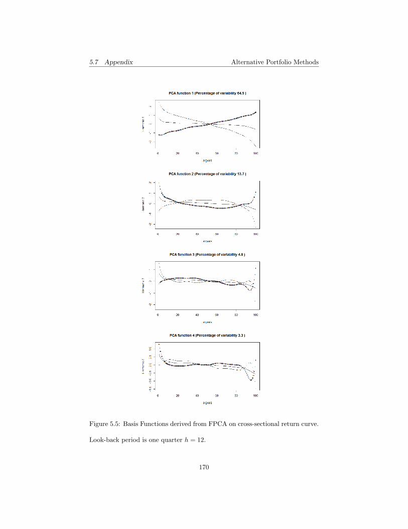
5.7 Appendix Alternative Portfolio Methods
Figure 5.5: Basis Functions derived from FPCA on cross-sectional return curve.
Look-back period is one quarter h = 12.
170

5.7 Appendix Alternative Portfolio Methods
Figure 5.6: Basis Functions derived from FPCA on cross-sectional return curve.
Look-back period is half year h = 26.
171

5.7 Appendix Alternative Portfolio Methods
Figure 5.7: Basis Functions derived from FPCA on cross-sectional return curve.
Look-back period is one year h = 52.
172

Alternative Portfolio Methods
6 Conclusion
The portfolio methods under investigation may be acclaimed in three circum-
stances. If market participants always make rational investment decisions, mod-
elling expected utility function should be of primary concern. Assumption of
CRRA functional leads to a favor for parametric portfolio, which gains addi-
tional out-of-sample stability from decomposition of weights. However, select-
ing factors with predictability requires a robust technique resistant to data-
snooping. I offer functional equivalence between predictive ability and prof-
itability of trading strategies. Thus, the bootstrap method enhances efficiency
of parameterized optimization by filtering out efficient indicators. An experi-
ment on FT100 shows promising performance of the mechanism.
Alternatively, mean-variance is recommended when input variables follow el-
liptical distribution. Although the condition is often violated on asset return,
many nonlinear trading strategies are able to produce valid training sample be-
fore feeding into optimizers. Another problem of plug-in method arises from
heterogeneous data generating process. Classifiers can then be applied in gath-
ering similar observations. My study shows that mean-variance can beat naive
strategy in constructing a portfolio of 24 commodity futures. But this outper-
formance is marginal after incorporating transaction cost.
In case that investors exhibit asymmetric aversion of tail risk, Choquet util-
ity maximization and coherent risk measures accquire superiority. It can be
shown that the scheme proposed by Koenker (2005) is equivalent to optimiza-
173

Alternative Portfolio Methods
tion using conditional value-at-risk (Rockafellar and Uraysev, 2000) both in
continuous and discrete cases. By decomposing quantile loss function, a new
parametric approach is proposed aiming at minimizing weighted downside risk
exposure on a set of factors given fixed target return. An empirical study on
comparing portfolio efficiency among mean-variance, pessimistic portfolio and
its parameterized version in global equity indices investment is then conducted.
Pessimistic portfolio offers the lowest return in frictionless environment, it also
suffers from overconcentration and non-stationarity of tail risk. Deterioration
of out-of-sample robustness can be possibly mitigated by stationary bootstrap
method but averaged performance barely beats benchmark. Parametric pes-
simistic portfolio effectively reduces tail risk exposure and data-snooping bias
in training samples and thus delivering a better risk-adjusted return.
Instead of utility maximization, an allocation policy can be formed by gaining
exposures on risk factors that are behaviorally priced. Trading factor port-
folio implicitly relies on the assumption that cross-sectional stock returns are
linearly correlated with market anomalies. I propose a test on functional de-
pendence using FPCA with linearity special basis function. It can be proved
that diversification benefit is always present as long as nonlinear components
are negligible. An experiment shows that momentum/mean-reversion accounts
for approximately 60% of return variation while quadratic function contributes
to 15% of that. Time series of scores, however, does not follow AR(p) process.
Finally, it is found that profitability of buy-winners-sell-losers is affected by
kurtosis of index return because investors require premium for extreme events.
174

Alternative Portfolio Methods
The bottom line of this research is that a portfolio choice only succeeds within
specific market conditions. Sustainable performance can be achieved by an ap-
propriate model on investor behavior and robust in-sample optimization tech-
niques.
175

REFERENCES Alternative Portfolio Methods
References
Abraham, C., Cornillon, P. A., Matzner-L?ber, E. R. I. C., and Molinari, N.
(2003). Unsupervised curve clustering using b-splines. Scandinavian journal
of statistics, 30(3):581–595.
Ait-Sahalia, Y. and Brandt, M. (1994). Variable selection for portfolio choice.
Journal of Finance, 56(4):1297–1351.
Ali, A., Hwang, L. S., and Trombley, M. A. (2001). Arbitrage risk and the
book-to-market anomaly. Journal of Financial Economics, 69(2):355–373.
Amaya, D., Christoffersen, P., Jacobs, K., and Vasquez, A. (2011). Do realized
skewness and kurtosis predict the cross-section of equity returns. School of
Economics and Management, University of Aarhus. No. 2011-44.
Ammann, M., S, O., and D., O. (2012). An alternative three-factor model for
international markets: Evidence from the european monetary union. Journal
of Banking & Finance, 36(7):1857–1864.
Anderson, T. W. (1963). Asymptotic theory for principal component analysis.
Annals of Mathematical Statistics, pages 122–148.
Ang, A., Hodrick, R. J., Xing, Y., and Zhang, X. (2006). The cross-section of
volatility and expected returns. The Journal of Finance, 61(1):259–299.
Ang, A., Hodrick, R. J., Xing, Y., and Zhang, X. (2009). High idiosyncratic
volatility and low returns: International and further us evidence. Journal of
Financial Economics, 91(1):1–23.
176

REFERENCES Alternative Portfolio Methods
Antoch, J., Prchal, L., Rosaria De Rosa, M., and Sarda, P. (2010). Electricity
consumption prediction with functional linear regression using spline estima-
tors. Journal of Applied Statistics, 37(12):2027–2041.
Apergis, N. and Payne, J. E. (2014). Resurrecting the size effect: Evidence from
a panel nonlinear cointegration model for the g7 stock markets. Review of
Financial Economics, 23(1):46–53.
Artzner, P., Delbaen, J., Eber, M., and Heath, D. (1999). Coherent measures
of risk. Mathematical Finance, 9:203–228.
Asness, C., Frazzini, A., and Pedersen, L. H. (2013). Quality minus junk.
Available at SSRN.
Asness, C. S. (1997). The interaction of value and momentum strategies. Fi-
nancial Analysts Journal, pages 29–36.
Banz, R. W. (1981). The relationship between return and market value of
common stocks. Journal of financial economics, 9(1):3–18.
Bassett, G., Koenker, R., and Kordas, G. (2004). Pessimistic
portfolio allocation and choquet expected utility. Available at
http://cemmap.ifs.org.uk/wps/cwp0409.pdf.
Bawa, V., Brown, S., and Klein, R. (1979). Estimation Risk and Optimal Port-
folio Choice. North Holland.
Berk, J. B. (1995). A critique of size-related anomalies. Review of Financial
Studies, 8(2):275–286.
177

REFERENCES Alternative Portfolio Methods
Bhandari, L. C. (1988). Debt/equity ratio and expected common stock returns:
Empirical evidence. The Journal of Finance, 43(2):507–528.
Black, F. (1972). Capital market equilibrium with restricted borrowing. Journal
of business, pages 444–455.
Black, F. and Litterman, R. (1992). Global portfolio optimization. Financial
Analyst Journal, 48(5):28–43.
Blitz, D., Huij, J., and Martens, M. (2011). Residual momentum. Journal of
Empirical Finance, 18(3):506–521.
Bouchaud, J. and Potters, M. (2009). Financial applications of random matrix
theory: A short review. working paper.
Brandt, M. and Santa-Clara, P. (2006). Dynamic portfolio selection by aug-
menting the asset space. Journal of Finance, 61:2187–2217.
Brandt, M., Santa-Clara, P., and Valkanov, R. (2009). Parametric portfolio poli-
cies: Exploiting characteristics in the cross-section of equity returns. Society
of Financial Studies, 22(9):3411–3447.
Brock, W., Lakonishok, J., and Lebaron, B. (1992). Simple technical trading
rules and the stochastic properties of stock returns. Journal of Finance,
47(5):1731–1764.
Cai, T. T. and Hall, P. (2006). Prediction in functional linear regression. The
Annals of Statistics, 34(5):2159–2179.
178

REFERENCES Alternative Portfolio Methods
Cakici, N., Fabozzi, F. J., and Tan, S. (2013). Size, value, and momentum in
emerging market stock returns. Emerging Markets Review, 16:46–65.
Carhart, M. M. (1997). On persistence in mutual fund performance. The Journal
of finance, 52(1):57–82.
Chan, L. K., Hamao, Y., and Lakonishok, J. (1991). Fundamentals and stock
returns in japan. The Journal of Finance, 46(5):1739–1764.
Chen, L., Novy-Marx, R., and Zhang, L. (2010). An alternative three-factor
model. Washington University in St. Louis, University of Chicago, and Uni-
versity of Michigan.
Claessens, S., Dasgupta, S., and Glen, J. (1995). The cross-section of stock
returns: Evidence from the emerging markets. World Bank Publications.
Cooper, M. J., Gulen, H., and Schill, M. J. (2008). Asset growth and the
cross-section of stock returns. The Journal of Finance, 63(4):1609–1651.
Cox, J. C. and Ross, S. A. (1976). The valuation of options for alternative
stochastic processes. Journal of financial economics, 3(1):145–166.
Daniel, K., Jagannathan, R., and Kim, S. (2012). Tail risk in momentum strat-
egy returns. National Bureau of Economic Research, No. w18169.
Daniel, K. and Moskowitz, T. J. (2013). Momentum Crashes. University of
Geneva.
Devlin, S. J., Gnanadesikan, R., and Kettenring, J. R. (1975). Robust estimation
and outlier detection with correlation coefficients. Biometrika, 62(3):531–545.
179

REFERENCES Alternative Portfolio Methods
Engle, R. (2002). Dynamic conditional correlation: A simple class of multivari-
ate generalized autoregressive conditional heteroskedasticity models. Journal
of Business and Economic Statistics, 20(3):339–350.
Eun, C. S. and Huang, W. (2007). Asset pricing in china’s domestic stock
markets: Is there a logic? Pacific-Basin Finance Journal, 15(5):452–480.
Fama, E. F. and French, K. R. (1992). The cross-section of expected stock
returns. the Journal of Finance, 47(2):427–465.
Fama, E. F. and French, K. R. (1993). Common risk factors in the returns on
stocks and bonds. Journal of financial economics, 33(1):3–56.
Fama, E. F. and French, K. R. (1998). Value versus growth: The international
evidence. The Journal of Finance, 53(6):1975–1999.
Fama, E. F. and MacBeth, J. D. (1973). Risk, return, and equilibrium: Empir-
ical tests. The Journal of Political Economy, pages 607–636.
Frazzini, A. and Pedersen, L. H. (2014). Betting against beta. Journal of
Financial Economics, 111(1):1–25.
Goia, A., May, C., and Fusai, G. (2010). Functional clustering and linear
regression for peak load forecasting. International Journal of Forecasting,
26(4):700–711.
Grinblatt, M. and Moskowitz, T. J. (2004). Predicting stock price movements
from past returns: The role of consistency and tax-loss selling. Journal of
Financial Economics, 71(3):541–579.
180

REFERENCES Alternative Portfolio Methods
Hall, P. and Hosseini-Nasab, M. (2006). On properties of functional princi-
pal components analysis. Journal of the Royal Statistical Society: Series B
(Statistical Methodology), 68(1):109–126.
Hiemstra, C. and Jones, J. D. (1994). Testing for linear and nonlinear
granger causality in the stock price-volume relation. The Journal of Finance,
49(5):1639–1664.
Hjek, J., ?idk, Z., and Sen, P. K. (1967). Theory of rank tests. New York:
Academic press.
Horvath, L. and Kokoszka, P. (2012). Inference for Functional Data with Ap-
plications. Springer Series in Statistics.
Hudson, R., Dempsey, M., and Keasey, K. (1996). A note on the weak form
efficiency of capital markets: the application of simple technical trading rules
to uk stock prices c 1935-1994. Journal of Banking and Finance, 20:1121–
1132.
Hyndman, R. J. and Ullah, S. (2007). Robust forecasting of mortality and
fertility rates: a functional data approach. Computational Statistics & Data
Analysis, 51(10):4942–4956.
James, G. M. and Hastie, T. J. (2001). Functional linear discriminant analysis
for irregularly sampled curves. Journal of the Royal Statistical Society: Series
B (Statistical Methodology), 63(3):533–550.
Jaschke, S. and Kuchler, U. (2001). Coherent risk measure and good deal
181

REFERENCES Alternative Portfolio Methods
bounds. Finance and Stochastics, 5:181–200.
Jegadeesh, N. and Titman, S. (1993). Returns to buying winners and selling
losers: Implications for stock market efficiency. The Journal of Finance,
48(1):65–91.
Jobson, J. and Korkie, B. (1980). Estimation of markowitz efficient portfolios.
Journal of American Statistical Association, 75(371):544–554.
Kendall, M. and Gibbons, J. (1990). Rank Correlation Methods. Oxford Uni-
versity Press.
Koenker, R. (2005). Quantile Regression. Cambridge University Press.
Kokoszka, P. and Reimherr, M. (2013). Predictability of shapes of intraday
price curves. The Econometrics Journal, 16(3):285–308.
Kraus, A. and Litzenberger, R. H. (1976). Skewness preference and the valuation
of risk assets. The Journal of Finance, 31(4):1085–1100.
Laloux, L., Cizeau, P., Potters, M., and Bouchaud, J. (2000). Random matrix
theory and financial correlations. International Journal of Theoretical and
Applied Finance, 3(3):391–307.
Lindberg, C. (2009). Portfolio optimization when expected stock returns are
determined by exposure to risk. Bernoulli, 15(2):464–474.
Lischewski, J. and Voronkova, S. (2012). Size, value and liquidity. do they really
matter on an emerging stock market? Emerging Markets Review, 13(1):8–25.
Markowitz, H. (1952). Portfolio selection. Journal of Finance, 7(1):77–91.
182

REFERENCES Alternative Portfolio Methods
Markowitz, H. (1959). Portfolio Selection: Efficient Diversification of Invest-
ments. Yale University Press.
Markowitz, H. (2012). Mean-variance approximations to expected utility. Eu-
ropean Journal of Operational Research.
Mas, A. (2007). Weak convergence in the functional autoregressive model. Jour-
nal of Multivariate Analysis, 98(6):1231–1261.
Mestekemper, T., Windmann, M., and Kauermann, G. (2010). Functional
hourly forecasting of water temperature. International Journal of Forecasting,
26(4):684–699.
Michaud, R. (1989). The markowitz optimization enigma: Is optimized optimal?
Financial Analyst Journal, pages 31–42.
Narayan, P. K. and Zheng, X. (2010). Market liquidity risk factor and financial
market anomalies: Evidence from the chinese stock market. Pacific-Basin
finance journal, 18(5):509–520.
Nartea, G. V., Wu, J., and Liu, Z. (2013). Does idiosyncratic volatility matter in
emerging markets? evidence from china. Journal of International Financial
Markets, Institutions and Money, 27:137–160.
Naughton, T., Truong, C., and Veeraraghavan, M. (2008). Momentum strate-
gies and stock returns: Chinese evidence. Pacific-Basin Finance Journal,
16(4):476–492.
Nicholas Refenes, A., Zapranis, A., and Francis, G. (1994). Stock performance
183

REFERENCES Alternative Portfolio Methods
modeling using neural networks: a comparative study with regression models.
Neural Networks, 7(2):375–388.
Penman, S. H., Richardson, S. A., and Tuna, I. (2007). The book-to-price effect
in stock returns: Accounting for leverage. Journal of Accounting research,
45(2):427–467.
Piotroski, J. D. (2000). Value investing: The use of historical financial statement
information to separate winners from losers. Journal of Accounting Research,
pages 1–41.
Pitas, I. and Venetsanopoulos, A. N. (1990). Nonlinear digital filters, volume 84.
Springer.
Pontiff, J. and Woodgate, A. (2008). Share issuance and cross-sectional returns.
The Journal of Finance, 63(2):921–945.
Qi, M. and Maddala, G. S. (1999). Economic factors and the stock market: a
new perspective. Journal of Forecasting, 18(3):151–166.
Quiggin, J. (1981). Perception and risk aversion among australian farmers.
Australian Journal of Agriculture Economics, 25:160–169.
Quiggin, J. (1993). Generalized Expected Utility Theory. Kluwer Academic
Publishers, Massachusetts.
Ramsay, J. and Silverman, B. W. (2005). Functional Data Analysis. Springer
Series in Statistics.
184

REFERENCES Alternative Portfolio Methods
Rockafellar, R. and Uryasev, S. (2000). Optimization of conditional var. Journal
of Risk, 2:21–41.
Rockafellar, R. and Uryasev, S. (2002). Conditional value-at-risk for general
loss distribution. Journal of Banking and Finance, 26:1443–1471.
Roll, R. and Ross, S. A. (1980). An empirical investigation of the arbitrage
pricing theory. The Journal of Finance, 35(5):1073–1103.
Salvage, L. (1954). Foundations of Statistics. Wiley.
Schmeidler, D. (1986). Integral representation without additivity. In Proceedings
of the American Mathematical Society, volume 97, pages 255–261.
Schmeidler, D. (1989). Subjective probability and expected utility without ad-
ditivity. Econometrica, 57:571–587.
Segovia-Gonzalez, M. M., Guerrero, F. M., and Herranz, P. (2009). Explaining
functional principal component analysis to actuarial science with an example
on vehicle insurance. Insurance: Mathematics and Economics, 45(2):278–285.
Sharpe, W. F. (1964). Capital asset prices: A theory of market equilibrium
under conditions of risk. The journal of finance, 19(3):425–442.
Shieh, S. J., Lin, C. Y., and Ho, P. H. (2012). Large changes in stock prices:
Market, liquidity, and momentum effect. The Quarterly Review of Economics
and Finance, 52(2):183–197.
Sood, A., James, G. M., and Tellis, G. J. (2009). Functional regression: A new
185

REFERENCES Alternative Portfolio Methods
model for predicting market penetration of new products. Marketing Science,
28(1):36–51.
Spearman, C. (1904). The proof and measurement of association between two
things. The American journal of psychology, 15(1):72–101.
Sullivan, R., Timmermann, A., and White, H. (1999). Data-snooping, technical
analysis trading rule performance, and the bootstrap. Journal of Finance,
54(5):1647–1691.
Tukey, J. W. (1960). A survey of sampling from contaminated distributions.
Contributions to probability and statistics, 39:448–485.
Von Neumann, J. and Morgenstern, O. (1944). Theory of Games and Economic
Behavior. Princeton.
Wang, Y. and Di Iorio, A. (2007). The cross section of expected stock returns
in the chinese a-share market. Global Finance Journal, 17(3):335–349.
White, H. (2000). A reality check for data-snooping. Econometrica, 68:1097–
1127.
Yao, F., Mller, H. G., and Wang, J. L. (2005). Functional linear regression
analysis for longitudinal data. The Annals of Statistics, 33(6):2873–2903.
Zhang, Y. (2011). Estimation of beta in a simple functional capital asset pricing
model for high frequency us stock data. Master Dissertation.
186