Embed Size (px)
Citation preview

Micro- and Macromixing Studies in Two- and Three-Phase
(Gas-Solid-Liquid) Stirred Chemical Reactors
by
Julia Hofinger
A thesis submitted to
The University of Birmingham
for the degree of
DOCTOR OF PHILOSOPHY
School of Chemical Engineering
University of Birmingham
August 2012

University of Birmingham Research Archive
e-theses repository This unpublished thesis/dissertation is copyright of the author and/or third parties. The intellectual property rights of the author or third parties in respect of this work are as defined by The Copyright Designs and Patents Act 1988 or as modified by any successor legislation. Any use made of information contained in this thesis/dissertation must be in accordance with that legislation and must be properly acknowledged. Further distribution or reproduction in any format is prohibited without the permission of the copyright holder.

ABSTRACT
The iodide/iodate reaction scheme was used to study the effect of gas sparging
and/or solid particles on micromixing in a stirred vessel. A literature review illustrated
the need for focused work on this matter and gave valuable ideas for the
experiments, especially considering the discrepancies reported in previous works.
However, the experimental method first had to be validated for the conditions with
added gaseous and solid phases air and glass beads, respectively. The experiments
covered a range of conditions for micromixing in single-phase, for validation, in gas-
liquid, solid-liquid and gas-solid-liquid systems: power inputs up to 1.94 W/kg, gas
sparge rates up to 1.5 vvm and up to 11.63 wt.% solids with diameters from 150 to
1125 . For comparison, the power inputs from the impeller were kept constant
when affected by the added phase(s).
The gas-liquid results clearly showed that micromixing for feeding near the surface
was significantly improved by gas sparging. In contrast, no changes were observed
near the impeller, when power input was kept constant. Near the surface the
contribution from the stirrer towards the local specific energy dissipation rate
becomes less dominant compared to the part from gas sparging. In addition, the
energy dissipated by the bursting of the air bubbles at the top might be an
explanation for the observed improvements.
In the solid-liquid cases low particle concentrations, i.e. up to 2.46 wt.%, showed no
significant effect when feeding near the surface, the impeller or . At 11.63 wt.%,
cloud formation occurred and micromixing was significantly worse near the impeller,
i.e. in the cloud, and near the surface above it, i.e. in the clear liquid layer.

Interestingly, this “dampening” was also found for larger solids which does not
indicate turbulence modulation due to the presence of the particles as had been
suggested in literature, but might point more towards energy dissipation due to
particle-particle interaction.
In addition to the two-phase work, gas-solid-liquid work is reported here which has
not been studied before. Due to the above results, low and high solids
concentrations were investigated over a range of gas sparge rates for feeding near
the surface and near the impeller. In contrast to the two-phase case, even small
amounts of particles gave slightly worse micromixing under sparged conditions.
Nevertheless, there were still improvements near the surface compared to the single-
phase data. For the sparged clouds, the results indicate some improvements
compared to the solid-liquid equivalents. However, this picture is more complex and
further information on the fluid flow in such systems is needed for detailed
discussion.
In order to allow better quantification of the experimental data, variations of the
Incorporation model were evaluated for taking recent suggestions for the reaction
scheme into consideration. The second dissociation of sulphuric acid was included
in the model and different kinetic rate laws from the literature on the Dushman
reaction were implemented. It was found that further kinetic data is needed for the
particular conditions in the experiments, but that the current variations allow order-of-
magnitude estimates and further comparisons of local specific energy dissipation
rates.

DEDICATION
To my family

ACKNOWLEDGEMENTS
I thank my main supervisors Dr. Waldemar Bujalski and Prof. Alvin Nienow for their
outstanding support throughout the project, while giving me plenty of freedom to
learn. Especially, Waldek’s technical understanding and experience in looking after
his many students were of great value. Moreover, working with Alvin was an honour
and in particular his knowledge and sense of humour made discussions much more
pleasant. In addition, I wish to acknowledge Dr. Serafim Bakalis who helped
especially in earlier stages of the project and offered many ideas for CFD work.
I am grateful for the full financial support from Huntsman Polyurethanes, Brussels. In
particular, the useful and friendly meetings with Dr. Archie Eaglesham and Dr.
Melissa Assirelli, who also gave great technical feedback, were just as helpful as the
sponsoring. I also thank them for giving me the opportunity to visit the site in
Everberg, Belgium, to work on some aspects of the project.
I want to acknowledge the IChemE Fluid Mixing Processes Subject Group for running
the research student competition. The prize for the first place 2011 was used for part
of the cost of attending ISMIP in Beijing. The experience was invaluable.
Moreover, a big “thank you” to the staff of the chemical engineering workshop,
especially Bob Sharpe: only such high quality technical support allowed me to obtain
accurate and consistent experimental results. Moreover, their friendship, the

encouragement served with afternoon teas and the spectacular Christmas parties will
be fond memories of this turbulent time at the University of Birmingham.
In addition to the workshop, I also want to thank the rest of the staff, especially Mrs.
Lynn Draper, for their great work which helped us focus on our studies.
For some of the CFD simulations, the university’s computer cluster, BlueBEAR, was
used and I wish to acknowledge the support from Paul Hatton and Aslam Ghurma. I
also want to thank Aslam for his help during my time on the postgraduate student
trainer team for CFX.
For their undergraduate projects, Yashar Khosrowyar, Yohann Mallet and Thibaut
Laurent helped with some of the experiments.
I have had the privilege and pleasure of meeting so many lovely people while being
here and it would be impossible to list them all. Therefore, I want to thank everyone
from 118 and G2, but also the CFD colleagues, especially Andrea, Dave and Lily, for
the great time and their friendship.
Last but not least, I am very grateful for my family’s support. Not only have they let
me go abroad, helped me financially and done lots of proofreading, but also their
encouragement and confidence in me has been fantastic. Thank you.

TABLE OF CONTENTS
1. Introduction .......................................................................................................... 1
1.1. Motivation and objectives ............................................................................... 1
1.2. Layout of thesis .............................................................................................. 2
2. Background and Literature ................................................................................... 4
2.1. Turbulent mixing in stirred vessels ................................................................. 4
2.1.1. A brief introduction to turbulence ............................................................. 4
2.1.2. Liquid mixing ............................................................................................ 8
2.1.3. Liquid-gas mixing ................................................................................... 12
2.1.4. Liquid-solid mixing ................................................................................. 15
2.1.5. Liquid-gas-solid mixing .......................................................................... 17
2.2. Micromixing .................................................................................................. 19
2.2.1. Mixing scales and chemical reactions .................................................... 19
2.2.2. Reaction schemes for experimental micromixing studies ...................... 22
2.2.3. Micromixing modelling ........................................................................... 25
2.3. Relevant studies in literature - What do we know already about the impact of
additional phases on turbulence and its impact on reactions? ............................... 32
2.3.1. Single phase .......................................................................................... 34
2.3.2. Possible effects of an added phase ....................................................... 35
2.3.3. With gas bubbles ................................................................................... 57
2.3.4. With solid particles ................................................................................. 59
3. Experimental method and its validation .............................................................. 65
3.1. The iodide/iodate method ............................................................................. 65
3.1.1. Reaction scheme ................................................................................... 65
3.1.2. Experimental procedure ......................................................................... 66

3.2. Experimental set-up ..................................................................................... 68
3.2.1. The rig ................................................................................................... 68
3.2.2. Adaptions for the reaction system .......................................................... 71
3.2.3. Sample taking and measurement of triiodide ......................................... 72
3.3. Validation of method - single-phase results .................................................. 73
3.3.1. Meso-/micromixing transition ................................................................. 73
3.3.2. Single-phase – comparison to literature ................................................ 75
4. Incorporation model: adaptation and its use to interpret experimental data ....... 78
4.1. Introduction .................................................................................................. 78
4.2. Materials and method ................................................................................... 80
4.2.1. Adapted model for the iodide/iodate method ......................................... 80
4.2.2. Kinetics .................................................................................................. 84
4.2.3. Numerical method .................................................................................. 91
4.2.4. Polynomial regression for quantitative comparison ................................ 92
4.3. Results and discussion ................................................................................. 93
4.3.1. Validation of the implemented model ..................................................... 93
4.3.2. Modelling results and use for interpreting experimental data ................. 96
4.3.3. Including dissociation and adapted kinetic model ................................ 108
4.3.4. Use of such models to compare data .................................................. 111
4.4. Conclusions ................................................................................................ 114
5. Micromixing in gas-liquid systems .................................................................... 115
5.1. Introduction ................................................................................................ 115
5.2. Validation of the experimental method for sparged conditions ................... 115
5.2.1. Loss due to gas stripping ..................................................................... 115
5.2.2. Oxidation of iodide ............................................................................... 117
5.3. Power input in sparged cases .................................................................... 117

5.3.1. Power measurement results in gas-liquid cases .................................. 117
5.3.2. Conditions for micromixing experiments with gas ................................ 119
5.3.3. Flow at the chosen conditions ............................................................. 119
5.4. Micromixing near impeller under gassed conditions ................................... 120
5.5. Micromixing near free surface under gassed conditions ............................ 126
5.6. Micromixing below impeller under gassed conditions................................. 129
5.7. Micromixing under gassed conditions without power input from impeller ... 132
5.8. Power input from gas ................................................................................. 134
5.9. Interpretation with micromixing model ........................................................ 135
5.9.1. General comparison ............................................................................ 136
5.9.2. Comparisons near surface ................................................................... 138
5.9.3. Comparisons near impeller .................................................................. 139
5.10. Conclusions ............................................................................................ 140
6. Micromixing in solid-liquid systems .................................................................. 141
6.1. Introduction ................................................................................................ 141
6.2. Validation of the experimental method in a liquid-solid system .................. 141
6.3. Power input in the presence of particles ..................................................... 142
6.3.1. Power measurement results in solid-liquid cases ................................ 142
6.3.2. Conditions for micromixing experiments with particles ........................ 143
6.3.3. Flow at the chosen conditions ............................................................. 145
6.4. Effect of particle size on micromixing in dilute suspensions ....................... 148
6.4.1. Near impeller ....................................................................................... 148
6.4.2. Near surface ........................................................................................ 151
6.4.3. Near location of highest energy dissipation rates, ..................... 153
6.5. Effect of solid concentration on micromixing .............................................. 156
6.5.1. Near impeller ....................................................................................... 156

6.5.2. Near surface ........................................................................................ 159
6.6. Interpretation with micromixing model ........................................................ 161
6.6.1. Effect of particle size at low particle concentrations ............................. 161
6.6.2. Effect of particle concentration (cloud formation) ................................. 162
6.7. Conclusions ................................................................................................ 164
7. Micromixing in liquid-gas-solid systems ........................................................... 166
7.1. Introduction ................................................................................................ 166
7.2. Power input in 3-phase (l-g-s) system ........................................................ 166
7.2.1. Power measurement results in liquid-gas-solid cases ......................... 166
7.2.2. Conditions for micromixing experiments with gas and particles ........... 168
7.2.3. Flow at the chosen conditions ............................................................. 169
7.3. Dilute, sparged suspension ........................................................................ 170
7.3.1. Near impeller ....................................................................................... 171
7.3.2. Near surface ........................................................................................ 173
7.4. Sparged cloud ............................................................................................ 177
7.4.1. Near impeller ....................................................................................... 177
7.4.2. Near surface ........................................................................................ 180
7.5. Interpretation with micromixing model ........................................................ 185
7.5.1. Dilute, sparged suspension ................................................................. 185
7.5.2. Sparged cloud...................................................................................... 187
7.6. Conclusions ................................................................................................ 191
8. Conclusions and future work ............................................................................ 193
8.1. Conclusions – discussed by chapter .......................................................... 193
8.2. Suggestions for future work ........................................................................ 195
References .............................................................................................................. 197
Appendices.............................................................................................................. 213

A. Calibration of triiodide measurement ............................................................. 213
B. Programme for solution of micromixing model – further details ..................... 215
C. Unbaffled stirred tanks - CFD ........................................................................ 216

LIST OF ILLUSTRATIONS
Figure 1: Pictures from early experiments on turbulence by injecting dye into the flow
through a pipe (Reynolds 1883) – (a) laminar and (b) turbulent ................... 4
Figure 2: Spectrum of eddies and their energy (Harnby et al. 1997) ........................... 7
Figure 3: Possible flow patterns in agitated vessels (Paul et al. 2004) ........................ 8
Figure 4: Typical power curves in single phase case for Rushton turbine (Harnby et
al. 1997) ....................................................................................................... 9
Figure 5: Local energy dissipation rates (normalised with ) in stirred tank – for
impeller region and bulk (Schäfer 2001) .................................................... 11
Figure 6: Flow transitions for gassed tanks (Nienow et al. 1985) .............................. 13
Figure 7: Typical power curve as a function of for a Rushton turbine under
gassed conditions (Harnby et al. 1997) ...................................................... 14
Figure 8: Stages of suspension of particles at high solid concentrations (solid line –
static solids; dotted line – interface suspended solids/liquid (Bujalski et al.
1999) .......................................................................................................... 16
Figure 9: Typical power input curves for three-phase system with Rushton turbine,
0.5 vvm air and various amounts of glass ballotini (Chapman et al. 1983a)
(X = mass percentage of particles)............................................................. 18
Figure 10: Macromixing time as a function of impeller speed (Rewatkar et al. 1991) 20
Figure 11: Transition between meso- and micromixing - effect of feed time on product
distribution – amended from Baldyga and Bourne (1992) .......................... 22
Figure 12: Selectivity towards side product, , as a function of Damköhler number
(Bourne 1997) ............................................................................................ 23

Figure 13: Schematic of formation of laminated structure due to vorticity (a) and
vortex stretching (b) (Baldyga and Bourne 1999) ....................................... 28
Figure 14: Incorporation between an aggregate of feed fluid 2 and bulk fluid 1
(Fournier et al. 1996a) ................................................................................ 31
Figure 15: Schematics showing particle distribution due to inertial clustering – left:
Eaton and Fessler (1994) – right: Sundaram and Collins (1997) ............... 37
Figure 16: Map of regimes of interaction between particles and turbulence
(Elghobashi 1994) ...................................................................................... 39
Figure 17: Image of the rig ........................................................................................ 69
Figure 18: Schematic of mixing tank and feed positions ........................................... 72
Figure 19: Effect of feed rate on segregation index – transition between meso- and
micromixing – feed position 2 (near impeller) ............................................. 74
Figure 20: Effect of feed rate on segregation index – transition between meso- and
micromixing – feed position 4 (near ) ................................................ 75
Figure 21: Segregation indices at 3 feed positions as a function of mean power input
– compared to results from similar experiments (Assirelli 2004) ................ 76
Figure 22: Comparison of the implemented routine to equivalent results from the
literature (Assirelli 2004)............................................................................. 94
Figure 23 : Comparison of results from the present model with those of Assirelli et al.
(2008b) at 3 acid concentrations ................................................................ 95
Figure 24: Species concentrations after dilution without reactions occurring ............ 96
Figure 25: Incorporation model with initially fully dissociated sulphuric acid and with
dilution implemented – kinetic data: Guichardon et al. (2000) .................... 97

Figure 26: Results for original model (fully dissociated) – compared to: with dilution
implemented using kinetic data by Schmitz (2000) .................................. 101
Figure 27: Results for original model (fully dissociated) – compared to: with dilution
implemented using kinetic data by Palmer and Lyons (1988) for I = 1M .. 102
Figure 28 : Kinetic rate constants obtained by Palmer and Lyons (1988) for three
ionic strengths and power law function fitted to data ................................ 103
Figure 29: Results for original model (fully dissociated) – compared to: with dilution
implemented using interpolated function of kinetic data by Palmer and
Lyons (1988) ............................................................................................ 104
Figure 30: Results for original model (fully dissociated) – compared to: with dilution
implemented using kinetic data by Xie et al. (1999) ................................. 105
Figure 31: Kinetic rate constants obtained by Palmer and Lyons (1988) and Xie et al.
(1999) for different ionic strengths and power law function fitted to data . 106
Figure 32: Results for original model (fully dissociated) – compared to: included
dissociation and adapted kinetic behaviour .............................................. 108
Figure 33: An example of the effect, with time, of air sparging at 1.0 vvm on the
absorbance, i.e. triiodide concentration, of a typical solution of reactants 116
Figure 34: Relative power demand as function of gas flow number – gassed ......... 118
Figure 35: as a function of mean specific energy dissipation rate at various
gassing rates – impeller feed with 1 mol/L ................................... 122
Figure 36: as a function of mean specific energy dissipation at varied gassing
rates – impeller feed with 0.5 mol/L ............................................. 123

Figure 37: Influence of aeration rate on segregation index at several levels of mean
specific energy dissipation rate as percentage of single-phase results –
impeller feed with 0.5 mol/L ......................................................... 124
Figure 38: as a function of impeller speed at varied gassing rates – impeller feed
with 0.5 mol/L .............................................................................. 125
Figure 39: as a function of mean impeller specific energy dissipation rate at
different gassing rates – surface feed with 0.5 mol/L ................... 127
Figure 40: Reduction of segregation index compared to the unsparged value at
several mean specific energy dissipation rates – surface feed with 0.5 mol/L
..................................................................................................... 128
Figure 41: as a function of impeller speed at different gassing rates – surface feed
with 0.5 mol/L .............................................................................. 128
Figure 42: as a function of mean specific energy dissipation at varied gassing
rates – feed below impeller with 0.5 mol/L ................................... 130
Figure 43: Influence of aeration rate on segregation index at several levels of mean
specific energy dissipation rate as percentage of single-phase results –feed
below impeller with 0.5 mol/L ...................................................... 131
Figure 44: as a function of impeller speed at varied gassing rates – feed below
impeller with 0.5 mol/L ................................................................. 132
Figure 45 : Effect of gassing – without power input from the impeller – on segregation
index in feed positions 1 (near surface) and 2 (near impeller).................. 133
Figure 46: Power number as a function of Reynolds number – with and without
500 µm particles ....................................................................................... 143
Figure 47: Example of cloud ( = 500 µm; 11.63 vol.%) ....................................... 147

Figure 48: Effect of particle size in dilute suspensions on the segregation index as a
function of particle concentration – near impeller at 660 rpm ................... 149
Figure 49: Effect of particle size in dilute suspensions at several particle
concentrations – in percent of single-phase segregation index – near
impeller..................................................................................................... 150
Figure 50: Effect of particle size in dilute suspensions on the segregation index as a
function of particle concentration – near surface ...................................... 151
Figure 51: Effect of particle size in dilute suspensions at several particle
concentrations – in percent of single-phase segregation index – near
surface ..................................................................................................... 153
Figure 52: Effect of particle size in dilute suspensions on the segregation index as a
function of particle concentration – near ........................................ 154
Figure 53: Effect of particle size in dilute suspensions at several particle
concentrations – in percent of single-phase segregation index – near
................................................................................................................. 155
Figure 54: Effect of particle concentration ( ) on segregation index – feed
position 2 (near impeller) .......................................................................... 157
Figure 55: Effect of particle concentration ( ) at low particle
concentrations as percent of single-phase segregation index – feed
position 2 .................................................................................................. 158
Figure 56: Effect of particle concentration ( ) at particle conc. with and
without cloud as percent of single-phase segregation index – feed position 2
................................................................................................................. 158

Figure 57: Effect of particle concentration ( ) on segregation index – feed
position 1 (near surface)........................................................................... 160
Figure 58: Relative power input as a function of gas flow number – gassed with
particles – 500 µm and 11.63 wt.% .......................................................... 167
Figure 59: Relative power input as a function of gas flow number – gassed with
particles – 1125 µm and 11.63 wt.% ........................................................ 168
Figure 60: Segregation index as a function of gassing rate in dilute suspension
(1.24 wt.%) - feed near impeller ............................................................... 171
Figure 61 : Effect of particle size and sparge rate on micromixing – in percent of
single-phase segregation index – near impeller ....................................... 172
Figure 62 : Effect of particle size and sparge rate on micromixing – in percent of gas-
liquid segregation index – near impeller ................................................... 173
Figure 63: Segregation index as a function of gassing rate in dilute suspension
(1.24 wt.%) - feed near surface ................................................................ 174
Figure 64 : Effect of particle size and sparge rate on micromixing – in percent of
single-phase segregation index – near surface ........................................ 175
Figure 65 : Effect of particle size and sparge rate on micromixing – in percent of gas-
liquid segregation index – near surface .................................................... 176
Figure 66: Segregation index as a function of gassing rate in dense suspension
(11.63 wt.%) - feed near impeller ............................................................. 178
Figure 67 : Effect of particle size and sparge rate on micromixing – in percent of
single-phase segregation index – near impeller ....................................... 178
Figure 68 : Effect of particle size and sparge rate on micromixing – in percent of gas-
liquid segregation index – near impeller ................................................... 179

Figure 69 : Effect of particle size and sparge rate on micromixing – in percent of
solid-liquid segregation index – near impeller .......................................... 180
Figure 70: Segregation index as a function of gassing rate in dense suspension
(11.63 wt.%) – feed near impeller ............................................................ 181
Figure 71 : Effect of particle size and sparge rate on micromixing – in percent of
single-phase segregation index – near surface ........................................ 182
Figure 72 : Effect of particle size and sparge rate on micromixing – in percent of gas-
liquid segregation index – near surface .................................................... 183
Figure 73 : Effect of particle size and sparge rate on micromixing – in percent of
solid-liquid segregation index – near surface ........................................... 184
Appendix figure 1: Calibration curve for extinction coefficient of triiodide ................ 213
Appendix figure 2: Segments of geometry for detailed structured meshing ............ 219
Appendix figure 3: Details of structured mesh – showing half of feed pipe ............. 220
Appendix figure 4: Simpler mesh using tetrahedral elements and inflation layers
around the boundaries, for general simulations ....................................... 220
Appendix figure 5: Power number as function of Re – CFD results for k-ε and SST
turbulence models and without turbulence model (laminar) ..................... 222
Appendix figure 6: Flow field in turbulent regime – turbulence model: SST gamma-
theta ......................................................................................................... 223
Appendix figure 7: Fl as function of Re – CFD results ............................................. 224
Appendix figure 8: Fl as function of Re – experimental data from literature (Dyster et
al. 1993) ................................................................................................... 224
Appendix figure 9: Surface shape from Nagata equation for 5 rps .......................... 225

Appendix figure 10: Development of surface shape with pressure field – contours:
pressure; vectors: force ............................................................................ 226
Appendix figure 11: Comparison of particle tracks .................................................. 227

LIST OF TABLES
Table 1: Gore and Crowe criterion applied to a stirred tank (geometry, as used in this
work) with ............................................................................ 45
Table 2: Stokes number criterion applied to a stirred tank example .......................... 54
Table 3: Concentration of reactants (mol/L) .............................................................. 66
Table 4: Geometric ratios of the stirrer and the vessel (T = 288 mm) ....................... 69
Table 5: Power number in liquid-only system – compared to literature ..................... 70
Table 6: Coordinates of the feed positions ................................................................ 72
Table 7 : Rate constants of Dushman reaction for three ionic strengths by Palmer
and Lyons (1988) ....................................................................................... 86
Table 8: Comparison of assuming full dissociation or including dissociation in model
for position 4 (near ) – using kinetics from Guichardon et al. (2000) . 98
Table 9: Comparison of assuming full dissociation or including dissociation in model
for pos. 2 (near impeller) – using kinetics from Guichardon et al. (2000) ... 98
Table 10: Comparison of assuming full dissociation or including dissociation in model
for pos. 1 (near surface) – using kinetics from Guichardon et al. (2000) .... 98
Table 11: Results for model considering dissociation of acid using kinetics from
Schmitz (2000) – at different feed positions at 0.18 W/kg ........................ 101
Table 12: Results for model considering dissociation of acid using kinetics from Palmer
and Lyons (1988) for I = 1M – at different feed positions at 0.18 W/kg .......... 102
Table 13: Results for model considering dissociation of acid using data from Palmer
and Lyons (1988) interpolated function for I – at different feed positions at
0.18 W/kg ................................................................................................. 104

Table 14: Results for model considering dissociation of acid using data from Xie et al.
(1999) – at different feed positions at 0.18 W/kg ...................................... 105
Table 15: Results for model considering dissociation of acid using data from Palmer and
Lyons (1988) and Xie et al. (1999) – at different feed positions at 0.18 W/kg ... 107
Table 16: Comparison of original model and new approach including dissociation and
using adapted kinetics - for position 4 (near ) ................................. 109
Table 17: Comparison of original model and new approach including dissociation and
using adapted kinetics - for position 2 (near impeller) .............................. 109
Table 18: Comparison of original model and new approach including dissociation and
using adapted kinetics - for position 1 (near surface) ............................... 109
Table 19: Summary of Φ at various locations at 0.18 W/kg – shows significant
differences, but consistent pattern in data ................................................ 111
Table 20: Relative comparisons of Φ in % of various locations at 0.18 W/kg – data
becomes more consistent than in Table 19 .............................................. 112
Table 21: Impeller speeds at several gassing rates for matching mean specific
energy dissipation rates ........................................................................... 119
Table 22: Superficial gas velocities ......................................................................... 120
Table 23: Power input from gas ............................................................................... 134
Table 24: Power input from compressible gas in percent of power from impeller.... 135
Table 25: Estimates for at pos. 1 (near surface) – using original model ............. 136
Table 26: Estimates for at pos. 2 (near impeller) – using original model ............ 136
Table 27: Estimates for at pos. 1 (near surface) – using adapted model ........... 137
Table 28: Estimates for at pos. 2 (near impeller) – using adapted model ........... 137

Table 29: Estimates for as % of equivalent single-phase value at pos. 1 (near
surface) – to highlight effect of sparging – using adapted model ............. 138
Table 30: Estimates for as % of lowest power input for sparged case at pos. 1
(near surface) – to highlight effect of impeller – using adapted model ..... 139
Table 31: Estimates for as % of equivalent single-phase value at pos. 2 (near
impeller) – to highlight effect of sparging – using adapted model ............. 139
Table 32: Estimates for as % of lowest power input for sparged case at pos. 2
(near impeller) – to highlight effect of impeller – using adapted model .... 140
Table 33: Impeller speeds for experiments with solid particles for
matching mean specific energy dissipation rates, ...................... 144
Table 34: Suspension state of 500 µm particles over range of power inputs -
expressed as percent of .................................................................... 146
Table 35: Suspension state at 660 rpm - expressed as percent of ................... 147
Table 36: Effect of cloud on micromixing near impeller ........................................... 159
Table 37: Effect of cloud on micromixing near surface ............................................ 161
Table 38: Effect of particle size on – pos. 4 (near ) - 3 vol.% - deviation of
compared to single-phase result .............................................................. 162
Table 39: Effect of clouds on – pos. 1 (near surface) ......................................... 163
Table 40: Effect of clouds on – pos. 2 (near impeller) ........................................ 163
Table 41: Impeller speeds for three-phase experiments with 11.63 wt.% for matching
mean specific energy dissipation rate, ........... 169
Table 42: Suspension state for dilute and dense suspensions over range of sparge
rates - expressed as percent of ...................................................... 170
Table 43: Effect of sparging in dilute suspensions on – average of particle sizes
compared to single-phase data – pos. 1 (near surface) ........................... 185
Table 44: Effect of sparging in dilute suspensions on – average of particle sizes
compared to gas-liquid data – pos. 1 (near surface) ................................ 186
Table 45: Effect of sparging in dilute suspensions on – average of particle sizes
compared to single-phase data – pos. 2 (near impeller) .......................... 187
Table 46: Effect of sparging in dilute suspensions on – average of particle sizes
compared to gas-liquid data – pos. 2 (near impeller) ............................... 187
Table 47: Effect of sparging in dense suspensions on – 500 particles –
compared to liquid-only data – pos. 1 (near surface) ............................... 188
Table 48: Effect of sparging in dense suspensions on – 1250 particles –
compared to liquid-only data – pos. 1 (near surface) ............................... 189
Table 49: Effect of sparging in dense suspensions on – 500 particles –
compared to gas-liquid data – pos. 1 (near surface) ................................ 189
Table 50: Effect of sparging in dense suspensions on – 1250 particles –
compared to gas-liquid data – pos. 1 (near surface) ................................ 189
Table 51: Effect of sparging in dense suspensions on – 500 particles –
compared to liquid-only data – pos. 2 (near impeller) .............................. 190
Table 52: Effect of sparging in dense suspensions on – 1250 particles –
compared to liquid-only data – pos. 2 (near impeller) .............................. 190
Table 53: Effect of sparging in dense suspensions on – 500 particles –
compared to gas-liquid data – pos. 2 (near impeller) ............................... 191
Table 54: Effect of sparging in dense suspensions on – 1250 particles –
compared to gas-liquid data – pos. 2 (near impeller) ............................... 191

Appendix table 1: Some reported values for the extinction coefficient of triiodide
[extended and amended from Guichardon and Falk (2000)] .................... 214
Appendix table 2: Power input for different liquid fill levels – calculated from torque on
impeller or walls and baffles or integrated εT ............................................ 223
NOTATION
Arabic
c concentration mol/L
C impeller clearance m
Da Damköhler number -
mixing Damköhler number -
D diameter of stirrer m
dp diameter of particle m
D diffusivity m2/s
E Engulfment rate 1/s
expression for chemical species -
F expression for change of species in Incorporation model
-
dimensionless flow number (or ) -
Flg gas flow number -
g(t) growth function -
H fill level of tank m
k constant for reaction rate (depends on reaction)
L or characteristic length m
N rotational speed of stirrer 1/s
P power W
Pa particle momentum number -
Po power number -
P...or Q... factors for Incorporation model -
Q discharge flow
Qg gas flow rate
gas flow rate in vvm volume of air/minute per volume of liquid in the tank

r radial distance from tank centre m
R pipe diameter m
reaction term for species j mol/L s
Re Reynolds number -
s dimensionless factor in Zwietering equation -
Sc Schmidt number -
St Stokes number -
T tank diameter m
t time s
tc critical time s
tm micromixing time s
u or velocity (instantaneous) m/s
mean velocity m/s
fluctuating velocity m/s
relative velocity m/s
terminal velocity m/s
V volume m
v velocity m/s
W impeller blade width m
x axial distance from jet exit m
X mass percentage of particles %
XS selectivity for side-product -
deviation of XS from reference %
Y yield -
YST maximum yield at total segregation -
z axial distance from tank bottom m

Greek
(local) specific energy dissipation rate W/kg
mean specific energy dissipation rate W/kg
maximum local specific energy dissipation rate – ensemble-averaged
W/kg
maximum local specific energy dissipation rate
W/kg
length scale of turbulent eddy m
or Kolmogorov length scale m
dynamic viscosity kg/m s (or Pa s)
kinematic viscosity m2/s
density kg/m³
characteristic mixing time s
characteristic reaction time s
Kolmogorov time scale s
ratio of local to mean specific energy dissipation rate
-
mass fraction -
Abbreviations
CFD computational fluid dynamics
DNS direct numerical simulation
EDD Engulfment – deformation – diffusion model
GMM Generalised Mixing Model
IEM interaction by exchange with the mean model
LDA/LDV laser Doppler anemometry/velocimetry
LES large eddy simulation
PIV particle image velocimetry

PM perfectly mixed
ST total segregation
RMS root mean square
RT Rushton turbine
VoF Volume of Fluid

Introduction – Motivation and objectives
1
1. INTRODUCTION
1.1. Motivation and objectives
Many industrially relevant fast chemical reactions have fast side-reactions which lead
to unwanted products. Such waste products can not only reduce efficiency of a
process, but also affect the quality of the actual product. In addition to working on
the chemistry of the process, improving micromixing, i.e. contacting of the reactants,
can lead to better results.
Examples of processes where micromixing becomes important:
fast competing parallel or consecutive reactions
particle size distribution in precipitation
molecular weight distribution in polymerisation
In single-phase systems, including stirred tanks, micromixing is well studied, see e.g.
Assirelli (2004) and valuable progress has been made with the use of reaction
schemes employing competing reactions like the Iodide/iodate reaction method.
Unfortunately, possible effects of gas bubbles and solid particles on micromixing are
still not fully investigated, let alone understood. Other well-established
measurements techniques for studying fluid flow and turbulence fields, like PIV or
LDA, are laser-based and, therefore, only of use at low concentrations of dispersed
phase. There is, however, a small, sometimes contradicting amount of work
available in literature on the effect of particles on micromixing and also on turbulence,

Introduction – Layout of thesis
2
but targeted work is needed for gas-liquid, solid-liquid and gas-solid-liquid stirred
chemical reactors.
Therefore, the aim of this work is to shed light on micromixing in a two- and three-
phase agitated tank at well-defined, not previously studied conditions using the
Iodide/iodate reaction scheme. This method has been found to give qualitatively
reliable results in single-phase cases which could be verified against results from
other methods, but some suggestions have been made recently to move it towards
more quantitative use. These ideas will be tested as well.
1.2. Layout of thesis
In order to achieve the above objectives, this thesis is structured as follows: First, the
background and the available relevant literature will be discussed in chapter 2. This
is necessary to establish which conditions should be studied and which factors might
need most attention. Chapter 3 gives details on the method and the experimental
set-up with its adaptations for this work. This section also includes single-phase
results which are used to validate the approach chosen and to give reference values
for the multi-phase results. In chapter 4, recent criticism on and suggestions for the
improvement of the Iodide/iodate method are addressed by extending a micromixing
model, the Incorporation model, to better describe the employed reaction scheme.
These changes to the modelling have not been reported before and could allow more
quantitative interpretation of experimental data. In chapter 5, the suitability of using
air with the Iodide/iodate reaction scheme is first validated and experimental
conditions are chosen. Then the effect of gas sparging on micromixing in stirred
tanks is studied in experiments and that data evaluated using the model variations

Introduction – Layout of thesis
3
from chapter 4. In chapters 6 and 7, the same is done for solid-liquid and gas-solid-
liquid systems, studying effects in a well defined system over a wider, more
industrially relevant range of conditions than in previous work. Finally, chapter 8
gives the conclusions of the work presented in the thesis and suggestions for future
work are added as well.
Background and Literature – Turbulent mixing in stirred vessels
4
2. BACKGROUND AND LITERATURE
2.1. Turbulent mixing in stirred vessels
In this work, micromixing in agitated tanks will be investigated through experiments
and using a model. As micromixing is closely linked to turbulence, relevant aspects
of the latter will be summarised first. Then, an overview of necessary background on
single- and multi-phase mixing in stirred vessels is given in the following sections.
2.1.1. A brief introduction to turbulence
In literature on mixing, a strong distinction is typically made between laminar and
turbulent flows (Harnby et al. 1997; Paul et al. 2004). Only the latter are relevant in
this study and, therefore, turbulence should be discussed here briefly. This might
seem fairly straight-forward considering that such phenomena are commonly found in
nature, in everyday life and in industry, from rivers, to stirring a cup of tea and many
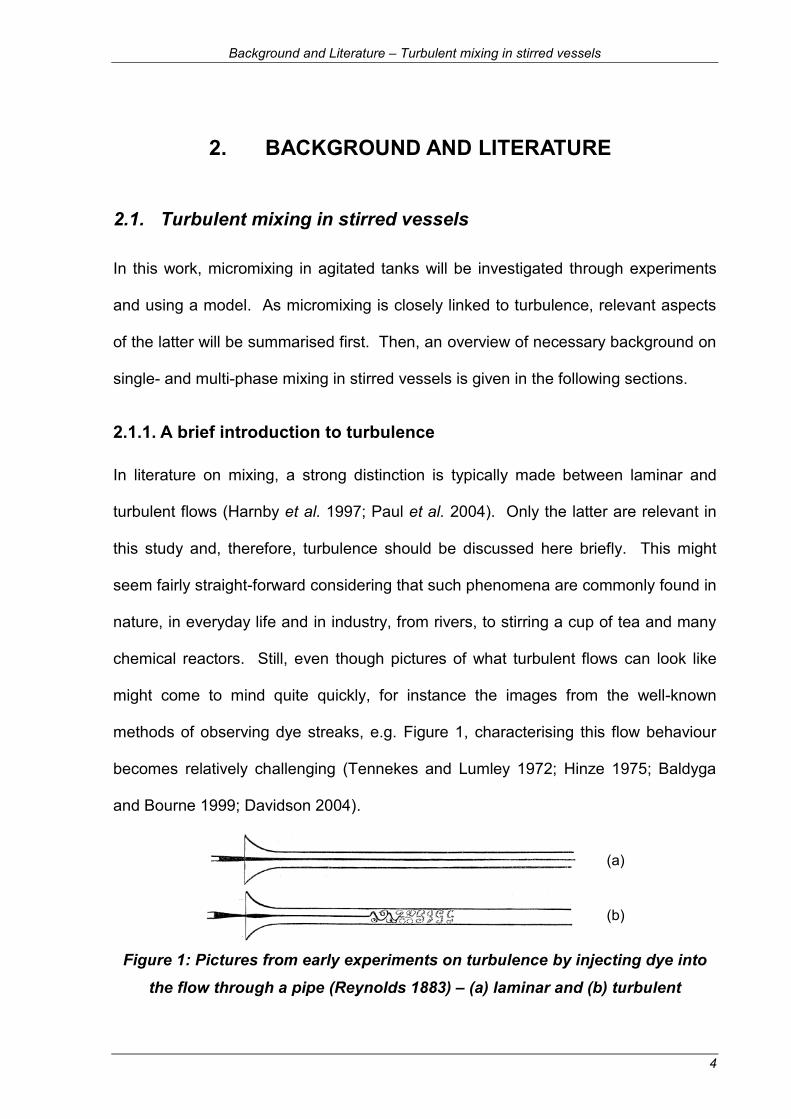
chemical reactors. Still, even though pictures of what turbulent flows can look like
might come to mind quite quickly, for instance the images from the well-known
methods of observing dye streaks, e.g. Figure 1, characterising this flow behaviour
becomes relatively challenging (Tennekes and Lumley 1972; Hinze 1975; Baldyga
and Bourne 1999; Davidson 2004).
(a)
(b)
Figure 1: Pictures from early experiments on turbulence by injecting dye into the flow through a pipe (Reynolds 1883) – (a) laminar and (b) turbulent

Background and Literature – Turbulent mixing in stirred vessels
5
In early work, Reynolds wrote that pipe flow “assumes one or other of two broadly
distinguishable forms-either the elements of the fluid follow one another along lines of
motion which lead in the most direct manner to their destination, or they eddy about
in sinuous paths the most indirect possible” (Reynolds 1883). Since then, some
more insight has been gained and for instance Tennekes and Lumley (1972) listed
the following characteristics to describe turbulence: irregularity, diffusivity, large
Reynolds numbers, three-dimensional velocity fluctuations, dissipation, continuum
(i.e. governed by equations of fluid mechanics); and turbulent flows are flows
(“Turbulence is not a feature of the fluids, but of fluid flows”). These ideas are often
referred to in literature to illustrate the complexities involved. Still, while turbulence
has been studied extensively, it is an open research topic (Clay Mathematics 2011)
and there are particular challenges in simulating such problems, although there are
useful models available. Plenty of texts (Davies 1972; Hinze 1975; Baldyga and
Bourne 1999; Davidson 2004) give excellent introductions to this extensive topic and
some variables and ideas are summarised here.
On practical terms, the Reynolds number, , which is defined as the ratio of inertial
and viscous forces, has been found useful for characterising flows:
(2.1)
With being the fluid density, L a characteristic length (for instance in a pipe the pipe
diameter), v the fluid velocity and is the dynamic viscosity. Low indicate laminar
flow, while the turbulent regime is characterised by higher . The transitional
behaviour between these regions can be complex (Saric et al. 2002).

Background and Literature – Turbulent mixing in stirred vessels
6
Because of the unsteady, 3-dimensional irregular behaviour of the flow, the
instantaneous velocity may be described by mean and fluctuating components:
(2.2)
This turbulent component is usually reported as root mean squared (or RMS) value
of the fluctuating velocities (Kresta 1998; Gabriele et al. 2009).
Some simplification is possible when the turbulent velocity fluctuations are, on
average, equal in all directions in space, i.e. when turbulence is isotropic. Assuming
such flow behaviour is of use for instance for computational fluid dynamics (CFD),
where a reduction of the number of variables in turbulence modelling allows faster
and computationally less expensive calculations. In contrast to isotropy, anisotropic
turbulence means that the different components are not equal, which can for instance
become relevant for instance near the wall of a pipe (Gore and Crowe 1991).
Turbulence is often described as a cascade of length scales where bigger eddies
give rise to smaller ones which again have smaller eddies until, on the smallest
scales, viscosity becomes dominant and energy is dissipated into heat (Richardson
1922; Argoul et al. 1989). In this approach, turbulence can be seen as a
superposition of spectrum of velocity fluctuations and eddy sizes (Nienow 1998).
Kolmogorov (1941) suggested that, at high Re, smaller turbulent eddies tend towards
isotropic behaviour, becoming independent from turbulence generation. Figure 2
shows such a range of different eddy sizes and their energy in turbulent flow for an
agitated vessel. The largest eddies on the left depend on the way they were
generated, e.g. in a stirred tank on the flow generated by the impeller; they are

Background and Literature – Turbulent mixing in stirred vessels
7
anisotropic and contain the most energetic eddies. The smaller ones are isotropic
and independent of the way the turbulent motion had been created. At the smallest
scales viscosity becomes dominant and the energy is dissipated into heat. On this
scale, which is named after Kolmogorov, where viscous and inertial forces are equal,
. From dimensional analysis, the Kolmogorov length scale can then be
obtained (Kolmogorov 1941):
(2.3)
This length scale is also indicated in Figure 2 and falls into the universal equilibrium
range, i.e. where eddies are do not depend on the way the turbulence has been
generated. This range can be divided into inertial sub-range, , and viscous
sub-range, . On the other side of the range are the larger eddies which
contain most of the energy; these most energetic eddies are often characterised by
the integral length scale, which is discussed in section 2.3.2. for agitated tanks.
Figure 2: Spectrum of eddies and their energy (Harnby et al. 1997)
Background and Literature – Turbulent mixing in stirred vessels
8
2.1.2. Liquid mixing
The Reynolds number, as introduced earlier, can be useful when describing the flow
in stirred vessels and is then defined with the impeller speed and diameter as
(2.4)
The flow is laminar at low Reynolds numbers, i.e. less than about 10, and turbulent at
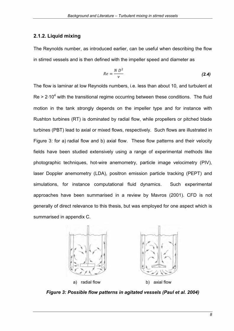
Re > 2∙104 with the transitional regime occurring between these conditions. The fluid
motion in the tank strongly depends on the impeller type and for instance with
Rushton turbines (RT) is dominated by radial flow, while propellers or pitched blade
turbines (PBT) lead to axial or mixed flows, respectively. Such flows are illustrated in
Figure 3: for a) radial flow and b) axial flow. These flow patterns and their velocity
fields have been studied extensively using a range of experimental methods like
photographic techniques, hot-wire anemometry, particle image velocimetry (PIV),
laser Doppler anemometry (LDA), positron emission particle tracking (PEPT) and
simulations, for instance computational fluid dynamics. Such experimental
approaches have been summarised in a review by Mavros (2001). CFD is not
generally of direct relevance to this thesis, but was employed for one aspect which is
summarised in appendix C.
a) radial flow b) axial flow
Figure 3: Possible flow patterns in agitated vessels (Paul et al. 2004)

Background and Literature – Turbulent mixing in stirred vessels
9
Such information on fluid velocities can be of use in assessing mixing performance.
For instance, the amount of fluid circulated by an impeller may help characterise a
mixing system. This internal circulation or discharge flow, , can be expressed by
the dimensionless flow number, :
(2.5)
Another important parameter is the power put by the impeller into the stirred vessel
which can be expressed with the dimensionless Power number, :
(2.6)
The power number is a function of Reynolds number, Froude number [second term in
equation (2.6)] and geometric ratios (D = impeller diameter, T = tank diameter, H = fill
level etc.). In addition, baffles, which can be installed to reduce gross vortexing,
significantly affect the flow field and consequently the power input. The plots of Po
vs. Re in Figure 4 show that the power number becomes constant in baffled vessels
at turbulent Reynolds numbers and that there are slopes of -1 in the laminar regime,
which reflects that viscous effects dominate the flow in the tank.
Figure 4: Typical power curves in single phase case for Rushton turbine
(Harnby et al. 1997)

Background and Literature – Turbulent mixing in stirred vessels
10
In the transitional region, the Power number of the Rushton turbine drops before
becoming a constant of about 5 in baffled and about 1 in unbaffled conditions. The
exact value of Po can be calculated for standard set-ups using empirical equations
which consider various geometric ratios, for instance Bujalski et al. (1987).
Experimentally, the power input into mixing devices has been investigated by
methods measuring temperature changes due to the energy dissipated in the fluid
(Kowalski et al. 2011), the power consumed by the motor, while taking potential
losses into account (Nagata 1975; Nienow et al. 1994), the torque transmitted from
the liquid to the vessel or the torque on the shaft (Nienow and Miles 1969; Bujalski et
al. 1987).
The specific power input or mean specific energy dissipation, , has long been
recognised as an important factor for mixing processes. For instance, gas-liquid
mass transfer depends, among other factors like for instance viscosity (Cooke et al.
1988), on the power input from the impeller (Van't Riet 1979; Nienow 1998):
(2.7)
Using only this mean value, however, might over-simplify reality as it fails to take into
account that the energy is not dissipated evenly throughout the stirred vessel. Earlier
measurements of local specific energy dissipation levels were done with
photographic technique (Cutter 1966) and hot-film/wire anemometry (Rao and
Brodkey 1972), also piezoelectric sensors (Fort et al. 1993) have been tried. More
recently, mainly laser-based methods have been used, i.e. laser Doppler
anemometry (LDA) or laser Doppler velocimetry (LDV) (Wu and Patterson 1989;
Ducci and Yianneskis 2005) and particle image velocimetry (PIV) (Baldi and
Yianneskis 2004; Gabriele et al. 2009).

Background and Literature – Turbulent mixing in stirred vessels
11
Such a distribution is shown in Figure 5 for a tank with a Rushton turbine (numbers in
figure indicate the feed positions used by the author for related micromixing studies
(Schäfer 2001)). The figure clearly illustrates that there are significantly higher
energy dissipation levels around the impeller compared to the bulk – in fact there is a
difference of orders of magnitude.
Figure 5: Local energy dissipation rates (normalised with ) in stirred tank –
for impeller region and bulk (Schäfer 2001)
Literature is in agreement that most of the energy is dissipated near the impeller;
nevertheless, absolute values vary considerably. For instance the highest local
specific energy dissipation rate, , often expressed as (i.e. to allow
comparison, has been found to be in the impeller discharge stream but values differ
significantly: in literature for the Rushton turbine has been reported ranging
from as low as around 8 (Bourne and Yu 1994) to moderate values of 52 (Schäfer
2001) or about 70 (Cutter 1966) and up to about 100 (Assirelli 2004; Assirelli et al.
Background and Literature – Turbulent mixing in stirred vessels
12
2008b). An explanation for these differences may be that the calculation of the local
specific energy dissipation rate from the raw LDA or PIV data or from micromixing
models is not straightforward – for optical methods (see Baldi and Yianneskis 2004;
Gabriele et al. 2009) and micromixing approaches (see Assirelli et al. 2008b).
Trailing vortices have been observed behind the impeller blades and, in the case of
the Rushton turbine, have been studied for a long time (Nienow and Wisdom 1974;
Van't Riet and Smith 1975). In this region of the flow, the highest local energy
dissipation levels or have been measured (Stoots and Calabrese 1995; Schäfer
2001), which is of use for understanding micromixing as discussed later (Assirelli et
al. 2002).
2.1.3. Liquid-gas mixing
In certain applications, e.g. many bio-reactions, gas is added to the system, often
using self-inducing impellers or spargers. Typical sparge rates for fermentations
might be around 0.5 to 1.5 vvm (Nienow 1998) and it is quite conceivable that the
gas might have a major impact on mixing and the fluid flow in the agitated vessel.
To quantify the amount of sparging, the gassing rate is often expressed as the
dimensionless gas flow number, , (which is in a similar form as the flow number
which is dependent on the flow generated by the impeller, Q, equ. (2.5)) with being
the gas flow rate:
(2.8)
When gassing rates are too high for given mixing conditions, “flooding” of the impeller
occurs. In this case, the flow in the tank is dominated by the gas flow, while

Background and Literature – Turbulent mixing in stirred vessels
13
macromixing and gas dispersion are poor (Nienow 1998; Paul et al. 2004) and,
therefore, this condition tends to be avoided. With increasing agitator speed, the
impeller becomes more significant for the bulk flow, which is referred to a “loaded”,
and the gas gets dispersed, first throughout the upper part of the tank. The transition
from flooding to loading occurs at the impeller speed, . At more intense agitation
conditions, above , complete dispersion is achieved, i.e. gas also reaches the
lower part of the vessel and circulates back to the impeller. At even higher impeller
speeds, recirculation becomes significant and the increased amount of gas which
collects in the trailing vortices behind the impeller can lower power input. Figure 6
illustrates the transitions from flooding to loading and to complete dispersion for a
Rushton turbine and other radial flow impellers.
Figure 6: Flow transitions for gassed tanks (Nienow et al. 1985)
These different flow regimes can not only be observed visually, but are also reflected
in the power input: It is well-known that the power number of many impellers drops
under gassed conditions (Cooper et al. 1944; Michel and Miller 1962; Joshi et al.
1982; Chapman et al. 1983c). For the Rushton turbine this drop can be 50% of the

Background and Literature – Turbulent mixing in stirred vessels
14
unsparged value, while some more modern impellers do not show such significant
reductions (Nienow 1996). Figure 7 shows the ratio of gassed to ungassed power
number for a Rushton turbine as a function of . The step at the right occurs at
high gas flow number, i.e. relatively high gassing rates with low impeller speed, and
shows the transition between flooding and loading. Then a minimum occurs in the
curve at from where the relative power input increases again until recirculation
becomes relevant at .
Figure 7: Typical power curve as a function of for a Rushton turbine under
gassed conditions (Harnby et al. 1997)
A main factor in the drop of power of the Rushton turbine are the low pressure
regions behind the impeller blades and its trailing vortices, which were introduced in
section 2.1.2.. It has been shown that gas tends to accumulate in different cavity
formations behind the blades which reduces the impeller’s effect and therefore
power.

Background and Literature – Turbulent mixing in stirred vessels
15
2.1.4. Liquid-solid mixing
Depending on the application of solid-liquid mixing, different degrees of suspension
or distribution of particles may be required. In some cases a homogenous
suspension might be the aim of the process, i.e. distributing the solids in the tank,
while in others it might only be necessary to get the surface area of all particles into
contact with the surrounding fluid, i.e. suspending them. For the latter problem, a
frequently used measure is the just suspended criterion where all particles are in
motion and no particles rest on the bottom of the tank for more than 1-2 seconds
(Zwietering 1958; Baldi et al. 1978; Harnby et al. 1997). For impeller speeds where
the particles are just suspended, , or above, the entire particle surface should be
available for the respective process.
Though probably difficult at larger scales, may be obtained experimentally
through visual observation of the tank’s bottom. In addition, various correlations for
the calculation of have been presented in literature. Probably the most well-
known one was suggested by Zwietering (1958) – for a particle concentration, ,
(mass solid/mass liquid x 100) and a particle diameter, :
(2.9)
Impeller speeds higher than might, however, be required to achieve a relatively
uniform distribution of solids throughout the tank (Chapman et al. 1983b).
Consequently, operation conditions will depend on the application. Further studies
on solid suspension, have found effects relevant to industry, e.g. Nienow (1968)

Background and Literature – Turbulent mixing in stirred vessels
16
showed the importance of impeller clearance in solid-liquid mixing. Still, Zwietering’s
correlation has been found useful and is widely employed (Paul et al. 2004).
At high solid concentrations, i.e. above about 10 wt.%, cloud formation has been
observed for certain conditions (Bujalski et al. 1999). In these cases, a cloud of
solids can be seen in the lower part of the tank near the impeller and a clear,
quiescent liquid in the region near the surface develops. This phenomenon has been
shown to significantly increase the mixing time for the bulk (macromixing defined in
section 2.2.1.), i.e. from a few seconds to minutes, though higher impeller speeds
can help improve mixing in such situations (Kraume 1992; Hicks et al. 1997; Bujalski
et al. 1999). The stages of cloud formation are illustrated in Figure 8 for increasing
impeller speeds – from most solids sitting on the bottom and the cloud at varying
heights to a more uniform distribution of the particles.
Figure 8: Stages of suspension of particles at high solid concentrations (solid line – static solids; dotted line – interface suspended solids/liquid (Bujalski et
al. 1999)
At low impeller speeds, higher amounts of solids can lower the power input
compared to the single-phase equivalent (Bujalski et al. 1999). An explanation for
this is that the particles are not suspended yet and get distributed at the bottom in a
“streamlined” shape which affects the flow while reducing the impeller clearance as
well (Bujalski et al. 1999). Lower amounts of particles, i.e. less than 10 wt.%, have
been shown to not significantly affect power input.

Background and Literature – Turbulent mixing in stirred vessels
17
2.1.5. Liquid-gas-solid mixing
In a sparged solid suspension a combination of the above effects might occur, i.e.
flow and power input might change significantly, but the interaction of particles and
bubbles might lead to additional complexity. Unfortunately, there is less information
available in the literature on such systems compared to two-phase ones.
Figure 9 gives an idea of how power input in three-phase stirred vessels is affected
by gassing rates and solid mass fraction. Overall, the trends resemble sparged
systems without added particles: power drops with increasing amounts of gas and
lower impeller speeds. Warmoeskerken et al. (1984) found that up to 5 wt.% did not
affect the gassed power input. However, at higher concentrations, like in Figure 9, it
can be seen that power tends to drop for instance with 20 or 30 wt.% when the
particles are not well suspended. Chapman et al. (1983a) explained this with the
distribution of the particles on the bottom of the tank; the power input is reduced due
to this false bottom as in the s-l case.

Background and Literature – Turbulent mixing in stirred vessels
18
Figure 9: Typical power input curves for three-phase system with Rushton turbine, 0.5 vvm air and various amounts of glass ballotini (Chapman et al.
1983a) (X = mass percentage of particles)
Regarding suspension, (for unsparged systems) tends to be lower than (with
gas) (Harnby et al. 1997; Kasat and Pandit 2005). For larger Rushton turbines
(D=T/2), the following equation has been proposed for estimating (Chapman et
al. 1983a; Bujalski 1986):
(2.10)
with being the gas flow rate in vvm (volume of air/minute per volume of liquid in
the tank). The data leading to equation (2.10) was obtained experimentally from 5
tank sizes, but further investigation might be of use.

Background and Literature – Micromixing
19
2.2. Micromixing
2.2.1. Mixing scales and chemical reactions
It can be useful to distinguish between mixing on different scales in the investigated
mixing equipment. First of these scales is macromixing. This is mixing on the
largest scales of the fluid flow, i.e. in the case of this work, the mixing vessel, and has
been studied extensively. It can be described by the macromixing or blend time,
which is a measure of how quickly an added substance will be dispersed throughout
the vessel. Therefore, it can be determined by adding a “tracer”, for instance with a
different pH, colour (change) or temperature, and observing when fluctuations in the
bulk fall below a specified threshold, e.g. 95% of the final value. This can be done
experimentally (Hiby 1979) and has also been attempted using CFD (Bujalski et al.
2002). Empirical relationships have been reported to allow calculation of blend times
in single-phase cases (Paul et al. 2004) and a strong dependence on power input
has been found (Nienow 1997; Kresta 1998).
In solid-liquid cases, macromixing time has been shown to be significantly worse
when clouds are formed, i.e. mixing time increased by up to more than two orders of
magnitude (Bujalski et al. 1999) – which means minutes instead of seconds for
blending a tank. In gas sparged stirred tanks, blend times have been found to drop
with increasing gas rates (Einsele and Finn 1980). Though, when compensating for
the reduction in power input, macromixing has been shown to be similar to single-
phase equivalents at mean specific energy dissipation rates (Saito et al. 1992). The
situation becomes more complex in gas-liquid-solid systems, but it has been shown
that gas sparging can improve macromixing at higher particle concentrations when
cloud formation occurs (Nienow and Bujalski 2002). An example for such conditions
Background and Literature – Micromixing
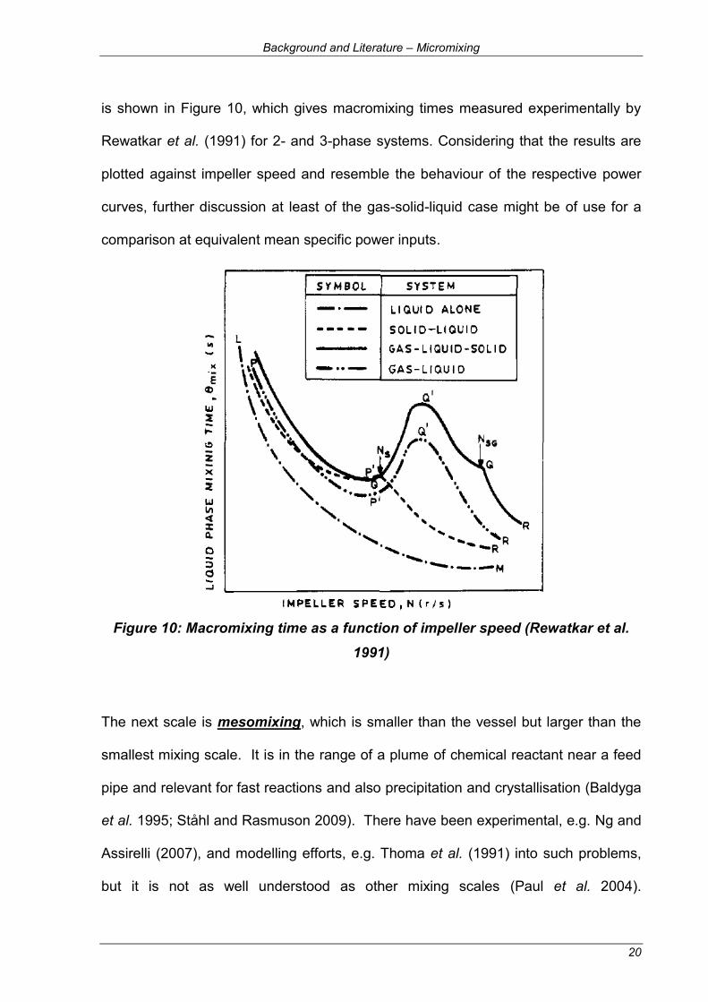
20
is shown in Figure 10, which gives macromixing times measured experimentally by
Rewatkar et al. (1991) for 2- and 3-phase systems. Considering that the results are
plotted against impeller speed and resemble the behaviour of the respective power
curves, further discussion at least of the gas-solid-liquid case might be of use for a
comparison at equivalent mean specific power inputs.
Figure 10: Macromixing time as a function of impeller speed (Rewatkar et al.
1991)
The next scale is mesomixing, which is smaller than the vessel but larger than the
smallest mixing scale. It is in the range of a plume of chemical reactant near a feed
pipe and relevant for fast reactions and also precipitation and crystallisation (Baldyga
et al. 1995; Ståhl and Rasmuson 2009). There have been experimental, e.g. Ng and
Assirelli (2007), and modelling efforts, e.g. Thoma et al. (1991) into such problems,
but it is not as well understood as other mixing scales (Paul et al. 2004).

Background and Literature – Micromixing
21
Nevertheless, mesomixing is not the focus of this work and further work in this field
would be necessary (Baldyga et al. 1997; Assirelli et al. 2011a).
The last step is micromixing which includes the smallest scale of fluid flow and also
diffusion. This obviously leads to mixing on the molecular level and can
consequently affect fast chemical reactions (Baldyga et al. 1995; Paul et al. 2004) –
e.g. when a very fast reaction competes with a fast side-reaction for the same
reactant, the product distribution can be affected by poor micromixing leading to local
over-concentrations of the added reactant, which might result in more side-product.
The transition between meso- and micromixing can be observed in experiments by
varying the feed time as illustrated in Figure 11. At high enough feed times (low feed
rates) the amount of side-product is not affected by the feed time, i.e. only
determined by micromixing. Below a critical feed time , the product distribution is
affected by the feed time which suggests that mixing on larger scales (mesomixing,
for example) becomes significant as well (Bourne and Thoma 1991; Baldyga and
Bourne 1992; Baldyga and Pohorecki 1995).

Background and Literature – Micromixing
22
Figure 11: Transition between meso- and micromixing - effect of feed time on
product distribution – amended from Baldyga and Bourne (1992)
In addition to these effects on different mixing scales, another aspect might become
relevant: under some conditions, i.e. too large feed pipe diameter or low feed rate,
fluid from the bulk might flow into the feed pipe which is called backmixing. Some
factors that might affect backmixing have been studied, but further work is needed
(Baldyga and Bourne 1993; Lee et al. 2007; Assirelli et al. 2011b).
The possible interactions of mixing and chemical reactions, can be evaluated by
comparing the time constants of the relevant processes. That relationship of mixing
and reaction is given in the Damköhler number for mixing, , which is the ratio for
characteristic mixing time, , and reaction time, , (Paul et al. 2004):
(2.11)
2.2.2. Reaction schemes for experimental micromixing studies
As (micro)mixing can affect fast chemical reactions, such reactions have been widely
used to study micromixing (Fournier et al. 1996b). These test reactions can be single
micro-mixing
meso-mixing

Background and Literature – Micromixing
23
reactions (A + B R) or competing reactions. The latter have the advantage that
the information on micromixing efficiency is retained in their product distributions, with
R being the primary, desired product and S the secondary (side-) product. They can
be divided into consecutive competing reactions (A + B R; R + B S) and parallel
competing reactions (A + B R; C + B S).
Figure 12 shows this dependence of the selectivity towards the side-product, , on
the Damköhler number. The amount of waste product increases with higher reaction
rate and with slower micromixing time. Therefore, it can be used to assess
micromixing efficiency qualitatively for the same reaction conditions and
quantitatively if the reaction kinetics are sufficiently well understood.
Figure 12: Selectivity towards side product, , as a function of Damköhler
number (Bourne 1997)
Many test reactions have been proposed over the years and the most important ones
can be found in several summarising tables by Fournier et al. (1996b).

Background and Literature – Micromixing
24
The most frequently used reaction schemes are the iodide/iodate method and the
“Bourne reactions”, several methods developed by J.R. Bourne and co-workers. To
the latter would belong, for instance, the azo-coupling of 1-naphthol with diazotized
sulphanilic acid (Bourne et al. 1981b). The iodide/iodate method was proposed by
Villermaux and co-workers to avoid problems found with other reactions like difficult
handling or toxic reactants (Fournier et al. 1996b). The reactions of the iodide/iodate
method are a neutralisation and a redox-reaction which compete for :
(2.12)
(2.13)
Unfortunately, also this reaction scheme has got at least one weakness: though it is
easy to use and gives qualitatively useful results, quantitative interpretation is difficult
due to unknowns regarding one of the reactions involved (Bourne 2008; Aubin et al.
2010). This will be discussed in section 2.2.3. and then an approach addressing this
issue will be tested in Chapter 4.
Taking all advantages and disadvantages of the range of available reaction schemes
into account, the iodide/iodate method was chosen for this study for the following
reasons:
safety
environmental and
economic considerations
option of performing successive injections, i.e. using a batch for more than
one injection (saves time and money, reduces waste)

Background and Literature – Micromixing
25
(expected) suitability for the planned multi-phase work, which was tested and
is reported at the beginning of the respective experiments
it also enabled a detailed comparison with extensive earlier similar work by
Assirelli (2004) but in single-phase systems.
The experimental setup and the method are described in Chapter 3.
2.2.3. Micromixing modelling
Motivation for micromixing modelling
The results from experimental studies can be used, when combined with micromixing
models, to give an indication of local specific energy dissipation rates (Bourne and
Yu 1994; Schaer et al. 1999); for instance Assirelli et al. (2008b) estimated local
specific energy dissipation rates at various feed positions in a stirred vessel. The
authors found that the ratio of the maximum local energy dissipation rate, to
the maximum ensemble-averaged energy dissipation rate was in reasonable
agreement with literature (Ducci and Yianneskis 2005), but that the absolute values
of were relatively high compared to results from LDA and PIV results. It was
suggested that a weakness in the model or in the kinetics might be the cause.
Recent literature (Bourne 2008; Kölbl and Schmidt-Lehr 2010) also points in this
direction and further work with modelling has been suggested as a solution. The
particular need for micromixing modelling with the iodide/iodate method will be
discussed further in the next section.
In addition to giving an estimate of local , micromixing models might be useful for
comparing experimental results: for example, the reactant concentrations employed
in the iodide/iodate reaction scheme may be altered for specific experimental

Background and Literature – Micromixing
26
conditions to enhance sensitivity to micromixing (Guichardon and Falk 2000). This
option also allowed the wide use of the method in various systems for instance to
study micromixers. Such changes, however, affect the reaction kinetics and make
comparisons between different concentrations more difficult (Assirelli et al. 2002).
Nevertheless, this has been done using segregation indices (Li et al. 2012), though
probably only to illustrate orders of magnitude. Therefore, micromixing modelling
could allow comparing results from different experiments and make the method more
versatile and quantitative.
Specific need for micromixing modelling with I/I method
As mentioned by Assirelli et al. (2008b), the reliability of the micromixing time, tm,
critically depends on appropriate modelling and realistic kinetics. Issues in this
respect might explain some qualitatively reasonable, but quantitatively unexpected
results reported by the authors. In fact, more doubts in this context have recently
been expressed in literature on the current approach: so far, the limiting specie, ,
has been provided by sulphuric acid in experiments and it has been assumed that it
is already initially fully dissociated (Guichardon and Falk 2000; Marchisio and Barresi
2003; Assirelli et al. 2008b). However, Bourne (2008) commented that the second
dissociation of sulphuric acid is not complete at the employed concentrations and
should consequently be considered in modelling the iodide/iodate reaction scheme.
Recently, Kölbl and Schmidt-Lehr (2010) have shown experimentally that sulphuric
acid and a stronger acid, i.e. perchloric acid, indeed do not give the same result, also
concluding that the dissociation needs to be included or suggesting the use of a
stronger acid. Interestingly, this might also explain the poor agreement between the
results from experiments and CFD simulations reported by Marchisio and Barresi

Background and Literature – Micromixing
27
(2003). A comparison of experiments and Comsol simulations of a hollow fibre
membrane device also only showed qualitative agreement (Baccar et al. 2009).
Moreover, discrepancies between results of very similar experiments (Schäfer 2001;
Assirelli et al. 2002) using different reactant concentrations might be – in part –
explained by this issue.
Therefore, in addition to the general motivation for micromixing modelling to obtain
information on local energy dissipation rates and to allow comparison between
different reactant concentrations, including the dissociation of sulphuric acid in a
model might aid quantitative use of the method.
On micromixing models
As with the chemical reaction schemes, a number of micromixing models have been
developed. There are also further options for CFD calculations (Fox 1998; Vicum
2005; Vicum and Mazzotti 2007), but only micromixing models are relevant to this
thesis.
Among several earlier models, ideas for the Interaction by exchange with the mean
(IEM) model were developed by several researchers independently (Harada et al.
1962; Costa and Trevissoi 1972b; Costa and Trevissoi 1972a; Villermaux and
Devillon 1972) as confirmed by (Villermaux and Falk 1994; Baldyga and Bourne
1999). It follows the concentration of a reactant at a point and, in addition to
chemical reaction, there is exchange with the mean surrounding environment. This
early model has been criticised (Baldyga and Bourne 1990) but still was found useful
for some applications (Fox and Villermaux 1990).

Background and Literature – Micromixing
28
A more complex model is the Engulfment, Deformation and Diffusion (EDD) model,
developed by Baldyga and Bourne (1984) and well-documented since then (Baldyga
and Pohorecki 1995; Baldyga and Bourne 1999). It describes the micromixing
process in 3 stages:
Engulfment: of reactant solutions into a vortex – see Figure 13 (a)
Deformation: of layers in lamellar structures – see Figure 13 (b)
Diffusion: of reactants in and between layers
(a) (b)
Figure 13: Schematic of formation of laminated structure due to vorticity (a) and vortex stretching (b) (Baldyga and Bourne 1999)
For (with Schmidt number kin. viscosity/diffusion coefficient)
and small amounts of feed compared to the bulk, engulfment has been shown to
become the limiting step and, consequently, the EDD model can be simplified to the
Engulfment model (Baldyga and Bourne 1989a). This simpler approach follows the
reactions and engulfment for a small volume of feed solution in to the bulk fluid. The

Background and Literature – Micromixing
29
growth of this volume is described by the Engulfment rate, E, and the change of
concentration of a substance α in this reaction region is (Baldyga and Bourne 1999):
(2.14)
with the first term describing the effect of engulfment, being the concentration of
in the bulk and in the reaction zone, and the second term accounting for the
reaction(s).
The engulfment behaviour was found to depend on local energy dissipation and
viscosity. The authors analysed turbulence spectra and found that the energetically
most active eddies, i.e. with the highest vorticity, are at a size around 12. From
this, a characteristic time scale could be obtained – for exponential growth of the
behaviour of the reacting zone was found to follow (Baldyga and Pohorecki 1995;
Baldyga et al. 1997):
(2.15)
The reciprocal value of E then gives a characteristic engulfment and, therefore, when
it is limiting, micromixing time.
The above form of the Engulfment model is only valid for low volume fractions of
added solution. Otherwise, interaction between the eddies of feed fluid, self-
engulfment, might need to be considered (Baldyga and Bourne 1999).
The E model requires less computation time, i.e. it is 1-2 orders of magnitude faster
to solve, than the EDD model (Baldyga and Bourne 1989a). Moreover, it has been
applied to stirred tanks successfully which is supported by experimental results
(Baldyga and Bourne 1990; Bourne and Yu 1994).

Background and Literature – Micromixing
30
Another, similar approach is the Incorporation model as developed and described by
Villermaux and his co-workers (Villermaux 1990; Villermaux et al. 1992). This was
found to be on an equivalent basis as the Engulfment model (Villermaux and Falk
1994). The Incorporation model was adapted for the Iodide/iodate method by
Fournier et al. (1996a) and has been employed in further studies (Fang and Lee
2001; Assirelli et al. 2008b). In these cases the product distribution could be
calculated for a range of micromixing times, , and the corresponding values then
used for interpretation of experimental data – for instance by employing equation
(2.15) for estimating energy dissipation rates from the obtained micromixing time.
A more universal model, the Generalised Mixing Model (GMM), was described by
Villermaux and Falk (1994), included the following mixing steps:
erosion of fresh fluid
dilution of the smaller eddies into the reacting zone
incorporation of bulk fluid into the reacting cloud
exchange or diffusion between small eroded and incorporated eddies in the
reacting cloud
The authors showed that the GMM includes other models like the IEM, the
Incorporation and Engulfment models as special cases.
Of the above models, the incorporation model was chosen for this work, because it
and the equivalent engulfment model have been shown to be suitable for such
applications, while being computationally less demanding than other options. In
addition, this approach had already previously been used with this reaction scheme

Background and Literature – Micromixing
31
(Fournier et al. 1996a; Assirelli et al. 2008b). Therefore, it is described in more detail
in the following section.
Incorporation model
As can be expected from its equivalence to the engulfment model, the incorporation
model is based on similar ideas and equations: Figure 14 shows a blob or aggregate
of fresh feed, fluid 2, as it slowly grows due to incorporation of surrounding fluid 1.
Figure 14: Incorporation between an aggregate of feed fluid 2 and bulk fluid 1
(Fournier et al. 1996a)
The characteristic incorporation time and the micromixing time, , are expected to
be the same. The growth behaviour of the aggregate is described by
(2.16)
In contrast to the engulfment model, this can but does not necessarily have to be
exponential growth, but can follow different functions g(t). Two suggested options
(Fournier et al. 1996a) would be linear with or exponential:
(2.17)
The concentrations of the different species can be described by considering the
effects of the incorporation and the chemical reaction(s):

Background and Literature – Relevant studies in literature - What do we know already about the impact of additional phases on turbulence and its impact on reactions?
32
(2.18)
The above repeatedly suggested similarity to the E model becomes apparent when
comparing equations (2.18) and (2.14). The details of the iodide/iodate reaction
scheme will be discussed in section 3.1. and further details on the implementation of
the model including the equations for all chemical species follow in section 4.2.1.
Calculating an independent value, like a micromixing time, e.g. the reciprocal value of
the Engulfment rate (Baldyga and Bourne 1999) or the incorporation time (Villermaux
and Falk 1994), should allow comparing results obtained from different reactant
concentrations. In addition, for quantitative or even just comparative use of the
Iodide/iodate method, the criticism and suggestions by Bourne (2008) and Kölbl and
Schmidt-Lehr (2010) have to be considered. Therefore, model variations following
these ideas will be evaluated in chapter 4.
2.3. Relevant studies in literature - What do we know already about
the impact of additional phases on turbulence and its impact on
reactions?
The effect of a dispersed phase, i.e. bubbles, drops or particles, on specific energy
dissipation rates in a turbulently flowing carrier fluid is of interest for various
(chemical) engineering applications, like multi-phase stirred tanks, bubble columns,
jet flows, pneumatic conveying and combustion, but also in other fields, for instance
higher in the atmosphere for studying cloud physics (Vaillancourt and Yau 2000) but

Background and Literature – Relevant studies in literature - What do we know already about the impact of additional phases on turbulence and its impact on reactions?
33
also under water for sediment transport and sand beds (Best et al. 1997). (In this
part of the text, “particles” will be used to include bubbles and drops.)
In spite of the subject’s wide relevance and considerable research efforts, it is still not
fully understood (Balachandar and Eaton 2010). Simulating the problem is
particularly challenging, as calculations of such flows, i.e. direct numerical
simulations (DNS) to resolve all turbulence scales, are computationally demanding,
especially at higher Reynolds numbers. Moreover, turbulent flows are still poorly
understood (Davidson 2004; Clay Mathematics 2011) and turbulence models, even
in single-phase turbulence, can be of limited use (Elghobashi 1994; Versteeg and
Malalasekera 2007). Sommerfeld and Decker (2004) mentioned in a review that
commercial CFD codes like Ansys CFX and Fluent do not offer options to include,
among other relevant effects, turbulence modulation due to the presence of particles
in multi-phase flow simulations. Nevertheless, calculations using such commercial
codes have been shown on occasions to give good agreement with experimental
results (Micale et al. 2000; Montante et al. 2001). Of course, better understanding of
these phenomena is needed for implementing them in mainstream software.
The purpose of the following section is to review relevant literature on the effect of
added second or third phases on turbulent flows, especially on turbulence modulation
and also micromixing in stirred vessels, will be discussed. Firstly, single-phase
operation, including open questions relating to unbaffled vessels, will be briefly
discussed to give a baseline and some background. Then phenomena involving
interaction of turbulence and a second, dispersed phase, especially turbulence
modulation will be introduced starting with literature on general fluid flow, though with
a specific focus on possible consequences for stirred tanks. Finally, modelling and

Background and Literature – Relevant studies in literature - What do we know already about the impact of additional phases on turbulence and its impact on reactions?
34
results from experiments on turbulence (modulation) and micromixing in gas-liquid,
solid-liquid and gas-solid-liquid stirred tanks will be reviewed.
2.3.1. Single phase
The distribution of turbulence parameters in stirred vessels has been measured for
many years, starting with Cutter (1966) who used a photographic technique. In
particular, he was the first person to show experimentally that the local specific
energy dissipation rate, , close to the impeller was much higher than the average;
whilst well away from the impeller near the extremities of the tank, was much less
than the average. The early work of Bourne and co-workers, e.g., Bourne et al.
(1981a), on micromixing in turbulent systems showed that it was the local value
that controlled the selectivity in fast chemical reactions, hence the importance of this
parameter.
Recently, turbulence has mainly been studied using LDA or PIV, which are much
more accurate techniques. However, the raw data still require significant data
treatment and a number of modelling assumptions to give information on the local
specific energy dissipation rates, (Kresta 1998; Unadkat et al. 2009b). That
treatment and model choices are not straightforward and can have a major impact on
the local values of estimated, as has been illustrated by Gabriele et al. (2009). In
addition to modern laser based measurements, micromixing experiments, in
combination with micromixing modelling, also allow estimations of local levels
(Bourne and Tovstiga 1988; Assirelli et al. 2002). Though both approaches, of
course, should essentially give the same value of at any location for each
particular flow system, they generally do not and each has some advantages and
some disadvantages. Optical methods actually try to measure the local and the

Background and Literature – Relevant studies in literature - What do we know already about the impact of additional phases on turbulence and its impact on reactions?
35
PIV technique can give more information, e.g. local data for a plane, than
micromixing experiments. The latter, on the other hand, assume that the reactions
that occur depend on the local , which is then obtained from a model, and therefore
the estimated value depends on a realistic model. In addition, it only measures at
the location of the reactant feed position. On the other hand, optical methods are
more likely to become problematic or even to fail in multi-phase and especially
opaque systems. Data treatment needs attention in both cases.
Figure 5 illustrated the well-established concept that the local specific energy
dissipation levels near an impeller are significantly higher than in the bulk of a liquid-
only, baffled, stirred vessel. Micromixing experiments using competing reactions
confirm this, as less side-product is formed when feeding close to the impeller
compared to feeding closer to or onto the liquid surface (Bourne and Yu 1994;
Villermaux et al. 1994; Schäfer 2001; Assirelli et al. 2002). Assirelli et al. (2005)
showed that continually feeding into the trailing vortices of a Rushton turbine using
rotating feed pipes gives even better micromixing.
2.3.2. Possible effects of an added phase
Suggested effects in the presence of particles
It is well-known that even small amounts of polymer additives can significantly
decrease drag, which is of use for instance in pipelines (Patterson et al. 1969; White
and Mungal 2008). In these cases, the pressure drop in pipes is lowered as well.
Similarly, such additives lower power input in stirred tanks too (Quraishi et al. 1976).
Also, solid particles have been observed, depending on the particle and flow
properties, like characteristic response times, enhancing or delaying the transition

Background and Literature – Relevant studies in literature - What do we know already about the impact of additional phases on turbulence and its impact on reactions?
36
from laminar to turbulent flow (Saffman 1962; Brennen 2005). These are examples
of possible effects of dispersed phases in (turbulent) fluid flows. In the following
section, further literature on turbulence - particle interaction effects which have been
shown to be relevant for stirred tanks will be discussed.
Preferential concentration – also called inertial clustering – is another well-recognised
aspect of particle - turbulence interaction which has been reported extensively
(Maxey 1987; Squires and Eaton 1991; Crowe et al. 1996; Balkovsky et al. 2001): it
has been shown that particles which are heavier than the fluid may accumulate in
regions of low vorticity, i.e. move away from eddies, while bubbles and lighter
particles tend to move towards intense vorticity, as can also be observed with
bubbles collecting in the trailing vortices of rotating impellers. Heavier particles will
be moved out of eddies due to their inertia and resulting centrifugal forces, while
lighter particles can follow such flows, as has been illustrated for instance by
Sundaram and Collins (1997) who used DNS – Figure 15 shows how particles may
be distributed due to inertial clustering: the circles and arcs represent the turbulent
eddies and the dots are particles; with the bigger ones getting centrifuged out of the
turbulent region.
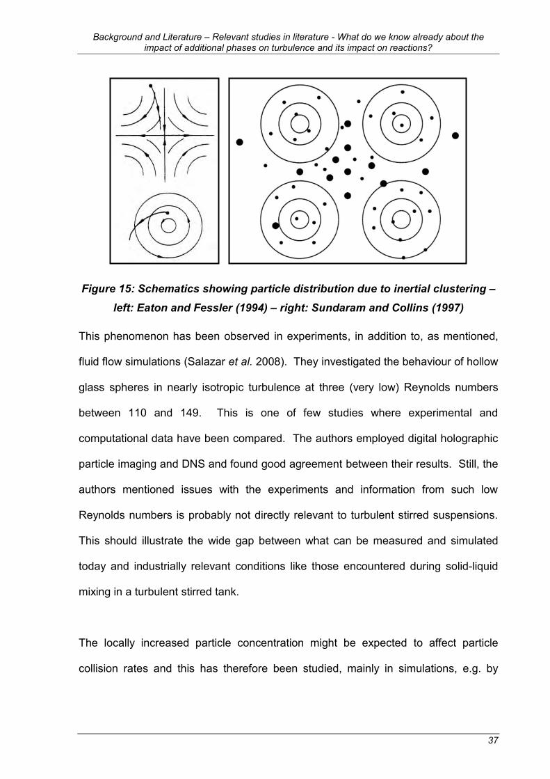
Background and Literature – Relevant studies in literature - What do we know already about the impact of additional phases on turbulence and its impact on reactions?
37
Figure 15: Schematics showing particle distribution due to inertial clustering – left: Eaton and Fessler (1994) – right: Sundaram and Collins (1997)
This phenomenon has been observed in experiments, in addition to, as mentioned,
fluid flow simulations (Salazar et al. 2008). They investigated the behaviour of hollow
glass spheres in nearly isotropic turbulence at three (very low) Reynolds numbers
between 110 and 149. This is one of few studies where experimental and
computational data have been compared. The authors employed digital holographic
particle imaging and DNS and found good agreement between their results. Still, the
authors mentioned issues with the experiments and information from such low
Reynolds numbers is probably not directly relevant to turbulent stirred suspensions.
This should illustrate the wide gap between what can be measured and simulated
today and industrially relevant conditions like those encountered during solid-liquid
mixing in a turbulent stirred tank.
The locally increased particle concentration might be expected to affect particle
collision rates and this has therefore been studied, mainly in simulations, e.g. by

Background and Literature – Relevant studies in literature - What do we know already about the impact of additional phases on turbulence and its impact on reactions?
38
Sundaram and Collins (1997) and Wang and Wexler (2000) who employed DNS. In
spite of recent advances, further work needs to be done in this field (Wang and
Wexler 2000).
The most relevant part of the existing body of published knowledge was reviewed by
Eaton and Fessler (1994) and more recently by Balachandar and Eaton (2010).
Interestingly, such locally increased particle concentrations, as described above for
simpler systems, were also reported for stirred solid-liquid systems, e.g. by Derksen
(2003) who performed LES of suspensions in an agitated vessel and Micheletti and
Yianneskis (2004) who employed LDA with a refractive index matching technique.
This phenomenon has nevertheless not been extensively studied for stirred tanks
and further research would be warranted.
In addition to being affected by the turbulent fluid flow, particles can also have effects
on the carrier fluid. Elghobashi (1994) gave an overview of these possibilities in a
graph which maps them with respect to particle volume fraction and relative particle
size, expressed as the ratio of characteristic times of fluid and solid (called Stokes
number which is discussed later). This graph is reproduced in Figure 16; it shows
that particles will not affect turbulence at very low concentrations, but that turbulence
can affect the dispersed phase. This is often referred to as one-way coupling and
inertial clustering, as discussed above, might be an example of such effects. At
higher concentrations, two-way coupling can be observed, i.e. particles may also
alter the fluid flow and its turbulence, in addition to being affected by it. When

Background and Literature – Relevant studies in literature - What do we know already about the impact of additional phases on turbulence and its impact on reactions?
39
particle concentrations increase even further, four-way coupling can be seen and
particle-particle interactions like particle-particle collisions become relevant.
Figure 16: Map of regimes of interaction between particles and turbulence
(Elghobashi 1994)
Moreover, Figure 16 shows that in two-way coupling particles may enhance
turbulence production or dissipation. This effect of dispersed solid phases on
turbulence in fluids has been studied extensively. Reviews of data from LDA and
some hot-wire anemometry experiments in pipe and jet flows suggest that “small”
particles suppress turbulence while “large” particles enhance turbulence (Gore and
Crowe 1989; Hetsroni 1989; Gore and Crowe 1991). Several parameters have been

Background and Literature – Relevant studies in literature - What do we know already about the impact of additional phases on turbulence and its impact on reactions?
40
proposed for determining the significant characteristics of “small” and “large”
particles, i.e. at which conditions the transition between attenuation and
augmentation occurs. Some of these suggested criteria are discussed below, though
it is worth mentioning that in most experimental work, relatively simple flow fields
have been studied and often air has been used as the continuous (often in such
studies called, carrier) phase, which might make comparisons to stirred tanks difficult.
Unfortunately, these phenomena are not fully understood yet, but a number of
mechanisms have been given in literature to explain the observed effects of particles
on turbulence (Brennen 2005; Balachandar and Eaton 2010).
In the book “Particles, bubbles & drops: their motion, heat and mass transfer”,
Michaelides (2006) suggested that the following mechanisms may contribute to
turbulence modulation in two phase mixtures:
a) Vortex breaking and dissipation of turbulence kinetic energy on the surface of
the immersed objects
b) Modification of the effective viscosity of the fluid
c) Eddy energy dissipated on the acceleration and deceleration of the elements
of the dispersed phase
d) Wakes and shedding of vortices behind the immersed objects
e) Fluid moving with the immersed objects or being displaced by them
f) Enhancement of the fluid velocity gradients between two neighbouring
immersed objects
g) Deformation and vibrations of the surface of the immersed objects

Background and Literature – Relevant studies in literature - What do we know already about the impact of additional phases on turbulence and its impact on reactions?
41
Of these points g) is not applicable for solid particles and f) and g) can usually be
neglected for low solid concentrations as well (Michaelides 2006).
Adding to these options, Ferrante and Elghobashi (2003) suggested explanations for
their unexpected results from simulations without gravity and with particles which
were smaller than Kolmogorov length scale. The calculations showed that small
particles might also produce the opposite of the usually observed effect: The authors
found increases in turbulent kinetic energy and energy dissipation levels. They
suggested that the particles might stay in the vortices which adds inertia and
consequently allows the vortices to stay stable for longer. In contrast, larger particles
would leave the eddies and enter new ones, creating counter-torques, which would
then reduce turbulence.
In a recent review (Balachandar and Eaton 2010), possible turbulence modulation
mechanisms were summarised as:
for suppression:
a) the enhanced inertia of the particle-laden flow
b) increased dissipation arising from particle drag
c) the enhanced effective viscosity of the particle-laden fluid
for enhancement:
d) enhanced velocity fluctuation due to wake dynamics and vortex-shedding
e) buoyancy-induced instabilities due to density variation arising from
preferential particle concentration

Background and Literature – Relevant studies in literature - What do we know already about the impact of additional phases on turbulence and its impact on reactions?
42
The authors (Balachandar and Eaton 2010) stated that sometimes several
mechanisms might, over a range of different scales, become relevant simultaneously.
They also added that current understanding still needs to be extended and that
contradictory results can be found in literature.
The last sentence also applies to such effects in stirred tanks, as will be discussed in
the following sections, 2.3.3. and 2.3.4.. These will cover experimental data from
stirred tanks and a distinction between added gaseous and solid phases is made, not
only because of the different density ratios compared to typical liquids, but also due
to different behaviour of particles compared to bubbles, which can deform and break
up and may coalesce. First, however, several suggested ways for determining the
transition between augmentation and suppression due to turbulence modulation are
discussed.
Transition criteria for turbulence modulation proposed in literature
A few parameters have been proposed for determining the transition of turbulence
modulation between suppression and enhancement. These will be introduced in the
following paragraphs with particular emphasis on possible application to flows in
stirred tanks. Such estimates might be useful for the interpretation of experimental
and modelling results.
Ratio of length scales – Gore and Crowe criterion
Gore and Crowe (1989) showed, based on an extensive literature review of
experimental data, that a ratio of characteristic lengths may be used for estimating
which turbulence modulating effect the added dispersed phase might have.
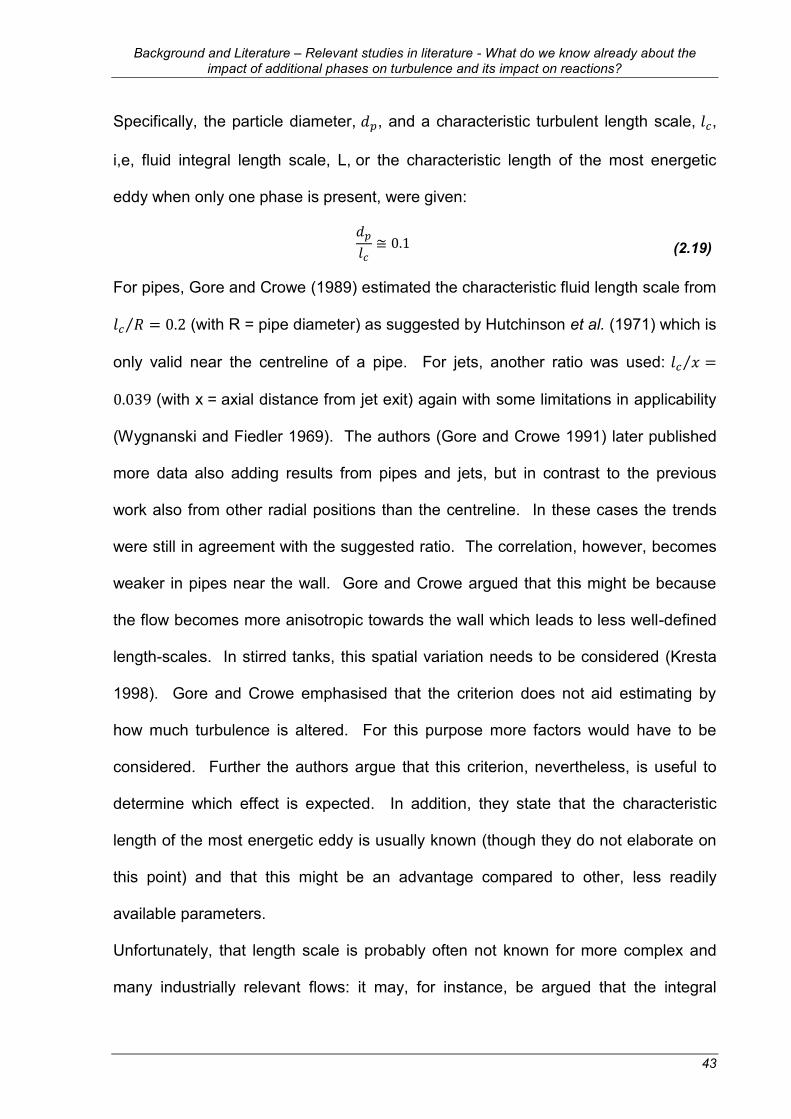
Background and Literature – Relevant studies in literature - What do we know already about the impact of additional phases on turbulence and its impact on reactions?
43
Specifically, the particle diameter, , and a characteristic turbulent length scale, ,
i,e, fluid integral length scale, L, or the characteristic length of the most energetic
eddy when only one phase is present, were given:
(2.19)
For pipes, Gore and Crowe (1989) estimated the characteristic fluid length scale from
(with R = pipe diameter) as suggested by Hutchinson et al. (1971) which is
only valid near the centreline of a pipe. For jets, another ratio was used:
(with x = axial distance from jet exit) again with some limitations in applicability
(Wygnanski and Fiedler 1969). The authors (Gore and Crowe 1991) later published
more data also adding results from pipes and jets, but in contrast to the previous
work also from other radial positions than the centreline. In these cases the trends
were still in agreement with the suggested ratio. The correlation, however, becomes
weaker in pipes near the wall. Gore and Crowe argued that this might be because
the flow becomes more anisotropic towards the wall which leads to less well-defined
length-scales. In stirred tanks, this spatial variation needs to be considered (Kresta
1998). Gore and Crowe emphasised that the criterion does not aid estimating by
how much turbulence is altered. For this purpose more factors would have to be
considered. Further the authors argue that this criterion, nevertheless, is useful to
determine which effect is expected. In addition, they state that the characteristic
length of the most energetic eddy is usually known (though they do not elaborate on
this point) and that this might be an advantage compared to other, less readily
available parameters.
Unfortunately, that length scale is probably often not known for more complex and
many industrially relevant flows: it may, for instance, be argued that the integral

Background and Literature – Relevant studies in literature - What do we know already about the impact of additional phases on turbulence and its impact on reactions?
44
length scale for instance in stirred tanks is not well-defined. As an approximation, a
value of 0.1 D or W/2 has been suggested, though higher values might be expected
for regions further away from the impeller discharge stream (Kresta and Wood 1993).
Also later, Kresta (1998) emphasised that the integral scale of turbulence changes
from the impeller to the bulk of the tank.
Various authors have reported values for the integral length scale and a few
examples will be given here to illustrate the general trend of the available data: Lee
and Yianneskis (1998) found 0.1 to 0.3 W in the impeller stream using LDA. They
added that the above mentioned estimate of the integral length scale being around
0.1 D could give an overestimation of L by a factor of 2 near the blade tip. Moreover,
Ducci and Yianneskis (2005) reported that the average integral length scale in the
vicinity of was around 0.05 D, i.e. about 50% of what would usually be expected
from the above estimates. Similarly, Gabriele et al. (2009), who normalised their
results against 0.1 D, found values from 0.2 near a pitched-blade turbine to 0.8
towards the wall, i.e. 20 to 80% of the estimate. In contrast, higher values have been
found in the bulk of the tank, e.g a range of 0.25 W near the impeller to 1-3 W in the
bulk (Costes and Couderc 1988). In a particularly careful study, Schäfer (2001) also
found significant differences between the region near the impeller and the bulk. He
suggested using different length scale values for these two parts of the vessel –
0.221 W for the impeller region and 0.333 T for the bulk, which is far away from
justifying the use of a constant value for the entire tank.
The examples given should illustrate that the integral length scale of turbulence may
vary throughout a stirred tank, i.e. an approximation with e.g. 0.1 D or W/2 could lead
to overestimation of L near the impeller and underestimation in the bulk. Therefore,
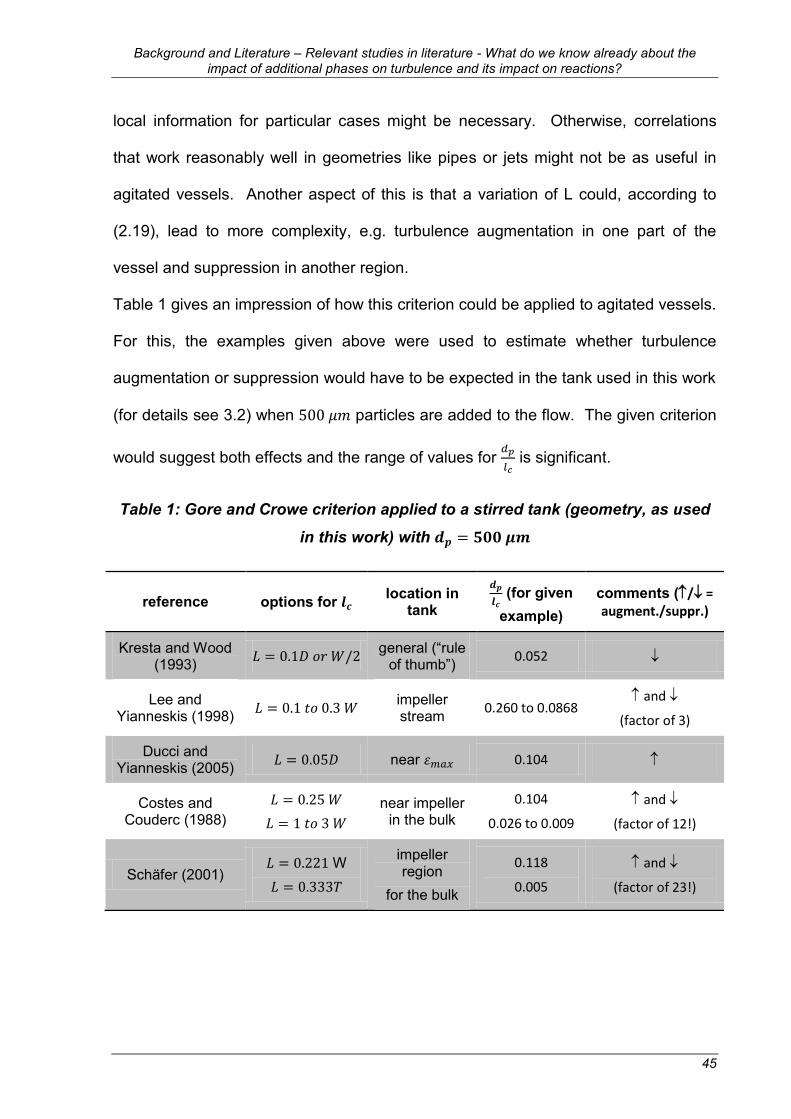
Background and Literature – Relevant studies in literature - What do we know already about the impact of additional phases on turbulence and its impact on reactions?
45
local information for particular cases might be necessary. Otherwise, correlations
that work reasonably well in geometries like pipes or jets might not be as useful in
agitated vessels. Another aspect of this is that a variation of L could, according to
(2.19), lead to more complexity, e.g. turbulence augmentation in one part of the
vessel and suppression in another region.
Table 1 gives an impression of how this criterion could be applied to agitated vessels.
For this, the examples given above were used to estimate whether turbulence
augmentation or suppression would have to be expected in the tank used in this work
(for details see 3.2) when particles are added to the flow. The given criterion
would suggest both effects and the range of values for
is significant.
Table 1: Gore and Crowe criterion applied to a stirred tank (geometry, as used in this work) with
reference options for location in
tank
(for given example)
comments (/ = augment./suppr.)
Kresta and Wood (1993) general (“rule
of thumb”) 0.052
Lee and Yianneskis (1998) impeller
stream 0.260 to 0.0868 and
(factor of 3)
Ducci and Yianneskis (2005) near 0.104
Costes and Couderc (1988)
near impeller in the bulk
0.104
0.026 to 0.009 and
(factor of 12!)
Schäfer (2001) W
impeller region
for the bulk
0.118
0.005
and
(factor of 23!)

Background and Literature – Relevant studies in literature - What do we know already about the impact of additional phases on turbulence and its impact on reactions?
46
Particle Reynolds number in stirred vessels
Hetsroni (1989) argued after reviewing literature, similar to Gore and Crowe’s
approach (1989), that the interaction between the particles and the fluid is based on
their size, relative velocity and density difference, which can consequently be
correlated using a particle Reynolds number, which the author suggested to define
as:
(2.20)
This definition of the Reynolds number deviates from that usually employed, as the
density and velocity differences between the phases and not the liquid density and
velocity are used. The author justified this definition because of the significant effects
of inertia and buoyancy on particle movements. In the actual argumentation,
Hetsroni (1989) did use the Reynolds number which only contains the fluid density
and based the review and interpretation of experimental data on that variable:
(2.21)
The author concluded that particles with a low particle Reynolds number tend to
suppress turbulence of the carrier fluid while particles with high particle Reynolds
number, , i.e. larger than about 400, tend to enhance the turbulence, which
Hetsroni (1989) suggested was probably due to vortex shedding. More recent work
suggests that the onset of vortex shedding depends on surrounding turbulence to
some extent (Balachandar and Eaton 2010). Hetsroni (1989) also added that further
experimental data was needed to quantify these effects.
Data on the velocity difference might not be available in some cases and other
formulations of the particle Reynolds number might need to be considered.

Background and Literature – Relevant studies in literature - What do we know already about the impact of additional phases on turbulence and its impact on reactions?
47
Fessler and Eaton (1999) studied turbulence modification by particles in a backward-
facing step flow and gave three options for the slip velocity in :
particle-fluid mean velocity difference
terminal velocity of the particles
fluctuating particle or fluid velocities
The authors concluded that all three options are suitable in their case, as all of them
are in the same order of magnitude. For other applications, this might not be true.
Moreover, velocity data is often not available to estimate values for the first and third
option. Therefore, the second suggestion, the terminal velocity, might be worth
considering and it indeed has been suggested: in their review, Poelma and Ooms
(2006) defined the particle Reynolds number as
(2.22)
with being the terminal velocity, i.e. the velocity a particle reaches when falling in
a quiescent fluid. The authors stated that can otherwise be defined using, e.g.,
the root-mean-square value of the free-stream turbulence as well.
It might be possible that such definitions using a different velocity could lead to
deviations from the original suggestion by Hetsroni (1989) and obtaining data like
RMS values might not be an option in many cases. In fact, the terminal velocity, i.e.
from a fluid at rest, could be determined quite easily. However, its use might not be
appropriate in the case of turbulent flows like in a stirred vessel, as it has been
shown that actual settling velocities tend to be much lower than expected. For
instance, Schwartzberg and Treybal (1968) reported settling velocities in an agitated
tank which were about 30-50% of the terminal velocity in a quiescent fluid. Also other
early experimental investigations (Levins and Glastonbury 1972; Nienow and Bartlett

Background and Literature – Relevant studies in literature - What do we know already about the impact of additional phases on turbulence and its impact on reactions?
48
1974) in stirred tanks also showed lower values and Brucato et al. (1998) even
observed a drop down to 15% in a study of a Taylor-Couette-flow. In addition to
reports of such measurements, correlations based on experimental data have been
proposed and relatively successfully employed in CFD simulations (Lane et al. 2004;
Doroodchi et al. 2008). Indeed, earlier simulations had shown the necessity of
considering the effects of turbulence on particle drag coefficients in such simulations
(Micale et al. 2000). Unfortunately, this significantly complicates the otherwise quite
simple approach for finding the transition between turbulence augmentation and
suppression by using the settling or terminal velocity to calculate the particle
Reynolds number.
In stirred tanks, as with the Gore and Crowe criterion, such calculations tend to
become less straightforward to implement compared to simple geometries like pipes
or jets. The relative velocity, as suggested by Hetsroni (1989), might be difficult to
use for many engineering problems where even detailed information on local single-
phase velocities might not be available, let alone multi-phase data. In some cases
lab-scale data might be available, but scale-up would still need to be considered. For
some problems, it might seem more feasible to obtain such information
computationally, for instance Ochieng and Onyango (2008) tested drag models in
CFD and could therefore get values for the relative velocities from their simulations.
Actually, apart from flow simulations, obtaining relative velocities for a given set-up
would require experimental investigation of the two-phase flow and consequently
would not help with reducing the need for such measurements.
Background and Literature – Relevant studies in literature - What do we know already about the impact of additional phases on turbulence and its impact on reactions?
49
Stokes number in stirred vessels
Another dimensionless expression, the Stokes number, has also been suggested for
characterising turbulence modulation (Owen 1969; Poelma and Ooms 2006).
The Stokes number is a measure of how faithfully a particle follows a flow or, in other
words, if it will follow a fluid flow around an obstacle or if it will hit the object. In many
cases and usually also in the context of turbulence modulation, it is defined as the
ratio of particle response time to fluid response time (Schetz and Fuhs 1996; Post
2010; Yeoh and Tu 2010):
(2.23)
This variable is in general relevant for investigating flows like those in stirred tanks,
as smaller numbers suggest that the particle will be strongly affected by the
surrounding fluid flow and that it may be used as a flow tracer, for instance in PEPT
(Fangary et al. 2000; Chiti et al. 2011) and PIV (Melling 1997; Unadkat 2009).
As it gives an idea of how strongly a particle will follow a flow, it is also frequently
used for describing preferential particle concentration due to inertial clustering which
is introduced above (see: Suggested effects in the presence of particles). It is quite
well-established that inertial clustering is strongest around (Squires and Eaton
1991; Balachandar and Eaton 2010). In this case, the particles will not follow the
flow perfectly, but will still be affected by it.
As suggested above, the Stokes number has also been employed in the context of
turbulence modulation, in addition to characterising inertial clustering. Therefore, a
closer look especially in the context of stirred tanks is warranted. For this variable

Background and Literature – Relevant studies in literature - What do we know already about the impact of additional phases on turbulence and its impact on reactions?
50
there are two aspects to consider: a) the critical value and b) the calculation of the
number. These are linked, of course, but will be discussed separately for clarity.
a) Critical value:
Owen (1969) argued that large particles with much higher relaxation times than
energy containing eddies would act more as fixed locations of resistance, while much
smaller ones would follow the turbulent motion. Therefore, the critical value would be
. Elghobashi (1994) (see Figure 16) followed this idea, but gave two Stokes
numbers, one for the integral scale and one using the Kolmogorov scale. The latter
had a critical value of 100 for a flow Reynolds number of 104. In recent studies
(Ferrante and Elghobashi 2003; Poelma and Ooms 2006) this definition of using the
Kolmogorov scale was followed too, but in these cases a value around 1 was found
critical, in contrast to the higher one of 100 indicated by Elghobashi (1994). In work
on stirred tanks, this definition has also been used with assuming the transition of
suppression and augmentation around unity (Gabriele et al. 2011). A recent review
(Balachandar and Eaton 2010) gives an overview of relevant studies, but the authors
do not find a clear critical value for turbulence modulation when using the Stokes
number.
b) Calculation of the Stokes number:
Owen (1969) was (one of) the first to propose the Stokes number for evaluating the
interaction between particles and a turbulent fluid flow, suggesting to calculate the
particle relaxation time, , according to Stokes’ law:

Background and Literature – Relevant studies in literature - What do we know already about the impact of additional phases on turbulence and its impact on reactions?
51
(2.24)
In Owen’s (1969) study, pneumatic phenomena were discussed, i.e. air was the
carrier phase – in stirred tanks it might make sense to use the density difference
instead of to take the more significant effect of buoyancy into account. Clearly,
this seems less relevant for the original case of air and heavier particles.
The author stated that Stokes’ law was sufficient in this case for simplicity and,
because he was concerned with orders of magnitude only. This needs consideration,
especially when taking the before mentioned settling behaviour into account.
Unfortunately, using Stokes’ law to characterise the particle behaviour might be
debatable, as it is – strictly speaking – only applicable for low around
0.1 (Rhodes 2008) or 1 (Micheletti and Yianneskis 2004) and, therefore, clearly does
not cover the range of interest in turbulence augmentation, for instance when vortex
shedding occurs at (Hetsroni 1989). Nevertheless, in some cases, finding
a suitable characteristic fluid time for complex flows like in stirred tanks could be a
bigger issue than the one for particles. Owen suggested using the characteristic time
of an energy-containing eddy for describing the fluid flow. Such large eddy time
scales, for instance the integral time scale, were employed by several authors
(Fessler and Eaton 1999; Sommerfeld 2001). In contrast, other authors calculated
the Stokes number considering the smallest turbulent eddies using the Kolmogorov
time scale as the characteristic fluid time (Ferrante and Elghobashi 2003; Poelma
and Ooms 2006), as mentioned for the critical value. This might, however, be
interpreted as a contradiction to Gore and Crowe (1989) who employed a
characteristic length scale of turbulence which usually is the integral length scale, i.e.
on the other extreme of the spectrum. If it can be shown that one of both length

Background and Literature – Relevant studies in literature - What do we know already about the impact of additional phases on turbulence and its impact on reactions?
52
scales works for predicting turbulence modulation in specific situations and another
criterion is useful in other cases, this might suggest different mechanisms, as listed
above, becoming relevant in those cases.
In stirred tanks, the Stokes number has been used as well and, while the calculation
of the particle response time has usually followed equation (2.24) (Fangary et al.
2000; Derksen 2003; Gabriele et al. 2011), there are several options for the fluid time
scale: Nouri and Whitelaw (1992), for instance, defined the single-phase flow
response time, based on blade width and impeller tip speed. Other workers (Fangary
et al. 2000; Chiti et al. 2011) used a fluid relaxation time based on impeller diameter
and, again, impeller tip velocity:
(2.25)
Derksen (2003) gave the Stokes number for particles in a stirred vessel as the ratio
of the Stokesian particle relaxation time, and the time of one impeller revolution:
(2.26)
Obviously, a comparison between these Stokes numbers would give different results
for the transition between turbulence suppression and augmentation in the same
system. Also, the integral time scale as proposed in literature on other flows (Owen
1969; Sommerfeld 2001) might be useful in stirred systems. Unfortunately, this could
be problematic due to the issues already discussed for the integral length scale. It
seems that choosing the flow response time is not straightforward in this case where
a wide range of time and length scales might be relevant – and affected.

Background and Literature – Relevant studies in literature - What do we know already about the impact of additional phases on turbulence and its impact on reactions?
53
However, the Stokes number has also been defined as the ratio of the particle time
scale and the Kolmogorov time scale by several authors (Elghobashi 1994; Poelma
and Ooms 2006) on particle-turbulence interaction. And, this definition has been
applied to particle-turbulence interaction in stirred tanks as well (Gabriele et al.
2011):
(2.27)
Sundaram and Collins (1997) chose this option too, but admitted that the choice of
the normalising scale is not obvious. Even though this might indeed be a reasonable
definition considering the importance of the smallest scale of turbulence for energy
dissipation and also for micromixing problems, good estimates of power input, let
alone local energy dissipation levels and consequently the Kolmogorov scales might
not be available in some systems. In addition, energy dissipation levels vary by
orders of magnitude in stirred tanks and, therefore, a Stokes number employing local
turbulence values might show different effects in different parts of the flow, as
mentioned for the ratio of length scales as well. Turbulence augmentation and
suppression occurring in the same vessel might be a possible scenario, but has so
far not been reported in literature (and would further complicate the issue).
The above gives an idea of the discrepancies in literature on defining the Stokes
number – from the time of rotation of the impeller, including or not, to integral time
scales or smallest turbulence time scales – and on the critical value. In such
complex flows, these options could lead to significantly different interpretation of
experimental or modelling data, as illustrated in Table 2. This example is a stirred
tank (geometry as used in this work, but with H=T) with N = 10 rps, Po = 5, water as

Background and Literature – Relevant studies in literature - What do we know already about the impact of additional phases on turbulence and its impact on reactions?
54
fluid and glass beads ( ) and estimating values for from literature data.
A critical value of was assumed, as other options would lead to more
confusion.
Table 2: Stokes number criterion applied to a stirred tank example
reference options
for
(using )
(using ) comments
(/=aug./sup.)
Fangary et al.(2000) Chiti et al. (2011)
1.09 0.66 and
Derksen (2003)
0.35 0.21
Gabriele et al. (2011) (conservative estimates: =50 (Schäfer 2001) =0.2 (Geisler and
Mersmann 1988))
363.02 ( )
22.96 ( )
51.34 ( )
218.25 ( )
13.80 ( )
30.86 ( )
(note variation between values)
Regardless of the above points, critical value and calculation of Stokes number, the
range of scales in stirred tanks, as shown for in Table 2, can complicate the use of
the suggested transition criterion.
Apart from the difficulties with the Stokes number discussed so far, another issue
was suggested by Gore and Crowe (1991) and later by Tanaka and Eaton (2008).
Gore and Crowe (1991) showed in a diagram the change of turbulence modulation
as a function of Stokes number and did not find good correlation. Tanaka and Eaton
(2008) plotted experimental results in a Re-St graph which did not give a clear picture
either and therefore, they argued that the Stokes number is (even) less useful for
determining the transition than the ratio of length scales proposed by Gore and

Background and Literature – Relevant studies in literature - What do we know already about the impact of additional phases on turbulence and its impact on reactions?
55
Crowe (1989). For this reason, Tanaka and Eaton (2008) introduced another
dimensionless number, the particle momentum number.
Particle momentum number – Pa
Recently, Tanaka and Eaton (2008) suggested a new expression, the particle
momentum number, Pa, as a criterion for determining the transition between
turbulence modulation effects. The dimensionless number was obtained from the
normalised Navier-Stokes in the presence of particles and can be expressed as a
function of Stokes and Reynolds number:
(2.28)
with being the large scale Reynolds number, the Kolmogorov length scale and
a (large scale) length scale. When plotting data from experiments in pipe and
channel flows, suppression was found for at and enhancement
occurring at higher and lower values (Tanaka and Eaton 2008; Balachandar and
Eaton 2010). Aside from , the authors gave a second particle momentum
number, , as an alternative:
(2.29)
which also contains and , the particle Reynolds number and diameter,
respectively, and the densities of the particle ( ) and the fluid ( ).
Tanaka and Eaton (2008) state that mass loading is relevant for the extent of
turbulence modification, but not a factor for the transition itself, as there are no
experiments where augmentation and suppression were observed depending on the
amount of particles. Interestingly, Unadkat et al. (2009a) did find changes over a
range of particle concentrations, though it may reasonably be argued that their

Background and Literature – Relevant studies in literature - What do we know already about the impact of additional phases on turbulence and its impact on reactions?
56
results at higher concentrations were already affected by particle-particle interaction
and not just two-way coupling anymore.
As the particle momentum number has only been introduced recently, further work
evaluating its limitations is needed. In addition, it might be difficult to use in poorly
characterised or complex flows as it requires values like the Stokes number or the
particle Reynolds number. Therefore, the issues mentioned above are also relevant
for the particle momentum number and its use for applications like stirred tanks might
be limited. Nevertheless, it is based on fundamental principles i.e. the Navier-Stokes
equations and an interesting, new approach which could and should be studied
further (Lohse 2008).
Conclusion for transition criteria
The above dimensionless numbers – ratio of length scales, particle Reynolds
number, Stokes number and particle momentum number – have been suggested in
consideration of the available data for turbulence modulation. In spite of the research
efforts in this direction, none of these options has actually been agreed on, let alone
become a well-established standard (yet). Moreover, a reasonable definition and
consequently calculation of such numbers for more complex flows than in pipes or
jets, as for instance in stirred tanks, might be problematic due to the wide range of
scales and turbulence intensities involved.
Once qualitative trends of turbulence modulation have been shown to consistently
agree with one criterion, quantitative estimates of the extent to which modification
occurs would be of interest for modelling tasks, especially for CFD. Further factors
like the effect of particle concentration or density differences will need to be
investigated as well.

Background and Literature – Relevant studies in literature - What do we know already about the impact of additional phases on turbulence and its impact on reactions?
57
One might, however, argue that it will be difficult to find one number which describes
the conditions in all parts of a stirred tank. Ratios containing local information, like
the particle Reynolds number, would at least allow a more flexible approach, but
would then require data which are very difficult to obtain.
In addition to determining the transition between enhancement and suppression in
general, there are also disagreements between experimental data for stirred tanks; a
brief review of available literature is given in the following sections.
2.3.3. With gas bubbles
As shown in part 2.1.3, sparging a stirred vessel with gas can strongly affect the
power input from an impeller and therefore the mean specific energy dissipation rate
(Chapman et al. 1983c; Harnby et al. 1997; Paul et al. 2004) – Figure 7. There is
less information on the effect of the presence of gas bubbles on local energy
dissipation levels and consequently micromixing in stirred vessels: Morud and
Hjertager (1996) reported velocity and RMS data for the gas phase using LDA/PDA
and used it to verify CFD results. Information on the distribution turbulence levels in
the liquid phase, however, was not given by the authors. PIV measurements from a
similar study of the liquid phase (Deen and Hjertager 2002) again are of limited use
in terms of micromixing for this study, as they are not at constant power input.
However, the authors did report effects of the gas on the fluctuating velocities which
could allow more detailed discussion of micromixing results. Also other studies using
various methods (Lu and Ju 1987; Khopkar et al. 2003; Khopkar et al. 2005;
Montante et al. 2008) do not aid understanding in this specific context, as they either
were focused on the general flow field or had relatively low gas sparge rates.

Background and Literature – Relevant studies in literature - What do we know already about the impact of additional phases on turbulence and its impact on reactions?
58
Measurements with a mechanical-piezoelectric sensor by Fort et al. (1993)
suggested that the gas flow significantly suppressed the local energy dissipation rate
in the impeller discharge flow and enhanced it in the rest of the vessel.
Unfortunately, such sensors probably have insufficient frequency response to make
accurate measurements of this parameter.
Bourne (1994), based on concepts of micromixing and results from diazo-coupling
experiments set out in the PhD thesis of Hilber (1987), reported that (subscript
g for “with gas”) near the impeller was not affected by gassing rates of up to 1.5 vvm
at constant power input, i. e., if . In that thesis (Hilber 1987), it was also
shown that micromixing near the surface was improved by sparging. On the other
hand, a similar study (Brilman et al. 1999) in a 0.7 L vessel also using diazo-coupling
found a negligible effect of sparging from ~ 0.5 to 10 vvm on micromixing, both near
the impeller and half way between it and the liquid surface at constant impeller
speed. This result is somewhat surprising as, at constant speed, and so
are the equivalent local values. Lin and Lee (1997) used the iodide/iodate reaction
scheme again in a small 1 L stirred vessel sparged at ~ 1.5, 10 and 20 vvm with
nitrogen and compared the results with those without sparging. They used various
impeller speeds (without power measurement) with three feed positions, two at the
height of the impeller and one close to the bottom of the vessel. They generally
reported improved micromixing but most of the experiments were conducted under
flooded conditions where, especially at the higher rates, the specific energy
dissipation rate from the sparged gas would have been greater than that from the
impeller. The latter condition may also have applied to the work of Brilman et al.
(1999) at the higher sparge rate. For the non-flooded conditions, Lin and Lee (1997)
Background and Literature – Relevant studies in literature - What do we know already about the impact of additional phases on turbulence and its impact on reactions?
59
found that when feeding the closest to the impeller, the XS values were generally
greater than the unsparged especially at the lower flow rate with little impact at the
higher rates. Data for the unsparged case were not reported for feeding near the
base so a comparison cannot be made for that location.
Two other relevant studies are those of Langheinrich and Nienow (1999) and
Boulton-Stone and Blake (1993). The former found that under flooded conditions,
sparging improved macromixing of material added to the top of a vessel when was
very low; whilst the latter showed that associated with bursting bubble but
very localised to them is many orders of magnitude greater than that from stirring.
Clearly, the impact of sparging on micromixing is unclear. Therefore, it was decided
to use the iodide/iodate method to study it, especially measuring the power input so
that agitator speeds giving could be selected, at a position near the
impeller where is high giving efficient micromixing in single-phase systems
(Assirelli et al. 2002), and near the surface, which is convenient for industry but not
effective for micromixing with Rushton turbines under unsparged conditions (though
the use of up-pumping impellers leads to a significant improvement as verified in
Bhattacharya and Kresta (2004)).
2.3.4. With solid particles
Direct measurements in stirred suspensions
In stirred solid suspensions, flow fields have been investigated experimentally at
sufficiently low concentrations, some with refractive index matching, that laser-based
techniques could be used. Mostly these studies have concentrated on the impeller
region. The first to measure the local specific energy dissipation rate, were

Background and Literature – Relevant studies in literature - What do we know already about the impact of additional phases on turbulence and its impact on reactions?
60
Geisler and Mersmann (1988). They used laser Doppler anemometry (LDA) with
refractive index matching and found that with 715 µm particles at 5 vol.% agitated by
a Rushton turbine, increased (but without any effect near the top surface).
More recently, Unadkat et al. (2009a; 2009b) using PIV have made similar
measurements for a pitched blade turbine with up to 0.5% by wt glass beads of 300,
750 and 1000 m. They found a reduction in very close to the impeller with
the 300 and 1000 m particles, the former giving the highest fall of ~ 25 %; and no
effect at 750 m. In spite of the problems with the Gore and Crowe criterion as
discussed above, they suggested that the suppression found with the 300 m
particles agreed with their criterion but on the other hand, the augmentation expected
for the larger sizes was, however, not found. Montante et al. (2010) using PIV
measured for 115 and 774 µm particles in the same region at up to 0.1 and
0.2% by volume, respectively. While the deviations of the mean flow field from the
single-phase results were negligible, was suppressed with the smaller
particles and enhanced by the larger ones. They concluded that their results agreed
with the Gore and Crowe criterion when estimating it from 0.1 (near the impeller) to
0.3 (towards the wall) D/4.
Other work has not measured directly but assessed turbulence in terms of
RMS velocities. For example, Guiraud et al. (1997) found that the axial and radial
rms velocities of the continuous phase from a down-pumping propeller were
unaffected by the presence of 253 m particles at 0.5 vol%. However, they observed
higher values in the axial RMS velocities for the particles. Later, Virdung and
Rasmuson (2007; Virdung and Rasmuson 2008) found that with a pitched-blade
turbine, rms enhancement occurred for 1, 1.5 and 2 mm particles again at 0.5%
Background and Literature – Relevant studies in literature - What do we know already about the impact of additional phases on turbulence and its impact on reactions?
61
volume, but also at 1 and 1.5%. In contrast to this, Micheletti and Yianneskis (2004)
using two sizes of Rushton turbines reported rms suppression in the impeller region
of the tank (which extended out to the equivalent feed point used here) by up to 70%
when dispersing 186 m particles, again at 0.5 vol%. Of these studies, only the latter
two were in agreement with the Gore and Crowe criterion as perceived by the
workers themselves. Complementary to such experimental work, CFD modelling
using large eddy simulation (LES) for liquid-solid suspensions with up to 3.6 vol.%
particle concentration of 300 and 470 m stirred by a Rushton turbine was published
by Derksen (2003). The turbulence levels were suppressed by the particles, more
strongly in the impeller stream than in other regions of the vessel. Interestingly,
locally increased solid concentrations near the impeller and especially in front of its
blades were observed in the simulations and have also been indicated
experimentally (Micheletti and Yianneskis 2004), which might be an explanation for
the large effects seen at such low solid concentrations. Clearly, though quite a lot of
work directly measuring turbulence in the presence of solids has been undertaken,
there is little agreement between the different studies; nor is there with the
interpretation of the Gore and Crowe criterion as perceived by each worker.
Over the last few years, new techniques have been developed which allow studies in
opaque systems and consequently at up to high particle concentrations, e.g. up to
19 wt.% using computer automated radioactive particle tracking (Guha et al. 2007) or
up to 40 wt.% using positron emission particle tracking (Guida et al. 2010). Such
techniques are not able to measure true turbulence parameters but do indicate very
little difference between the velocity of the fluid with and without particles present when
the concentrations are low, i.e. around 0.5 to 5 wt.% (Pianko-Oprych et al. 2009).

Background and Literature – Relevant studies in literature - What do we know already about the impact of additional phases on turbulence and its impact on reactions?
62
Micromixing in stirred suspensions
In addition to turbulence measurements, macro- and micromixing studies have also
been undertaken. As discussed in section 2.1.4., macromixing time is strongly
affected by the presence of more than about 10% granular solid particles, which
leads to ‘solid cloud formation’ in the lower part of the vessel above which a clear
layer of liquid appears (Bujalski et al. 1999). Under these conditions, the fluid above
the ‘cloud’ is very quiescent and the macromixing time, which is especially linked to
that region, maybe up to two orders of magnitude longer than without solids present.
The iodide/iodate method was first used to investigate micromixing in the presence of
glass particles (Villermaux et al. 1994; Guichardon et al. 1995). Initially, enhanced
micromixing was reported, but after correcting for loss of iodine during filtration
(Guichardon et al. 1995), the effect on micromixing for up to 6 wt.% for a range of
particle sizes from 20 to 1300 m was found to be negligible. Barresi (1997)
investigated the effect of glass spheres of ~ 175 and 450 m and also of 3mm
diameter cylindrical PET beads of low density up to 13 vol.% using a Rushton turbine
in a closed vessel to avoid any air ingestion and feeding above the impeller
approximately ¼ of the way to the top surface. They employed a reaction scheme
developed by Bourne and Yu (1994). At the lower concentrations with the beads at 2
and 7 vol% and with the PET particles at all concentrations, the selectivity was not
affected. At the higher concentration, ‘cloud’ formation was observed and feeding
into the ‘cloud’ led to a marked increase in selectivity, i.e. poorer micromixing. Later
Barresi (2000) used the same equipment with the same feed position but with a lower
level in the tank with both a down-pumping pitched blade turbine and a Rushton
turbine. They also used similar sized glass beads plus barite sand the size of the

Background and Literature – Relevant studies in literature - What do we know already about the impact of additional phases on turbulence and its impact on reactions?
63
smaller glass beads but of higher density (4280 compared to 2450 kg/m3) at 12 and
18 vol %. They also measured the power input and adjusted the impeller speeds to
give the same value with and without solids. With the Rushton turbine, cloud
formation was found in the earlier study and selectivity increased (Barresi 1997); in
the later study with the lower liquid level, it did not occur and selectivity was generally
unaltered. With the pitched blade turbine, cloud formation was found in every case
and the selectivity was increased by about 20 to 50%. Brilman et al. (1999) used
azo-coupling for investigating several feed positions but some very close to the
impeller but none near the top surface where clear liquid would be found if ‘cloud’
formation occurred. They used various sizes of glass beads from 30 to 700 m and
solid concentrations from about 2.5 up to 40 wt.% agitated by a Rushton turbine.
They found when feeding at approximately the mid-point between the impeller and
the upper surface that selectivity increased with increasing solid concentration except
with beads of ~ 300 m which did not have any effect. At a concentration of about
23 wt. %, the increase depended on particle size, with a minimum at ~ 300 m where
the effect was very small. Though they made no comment about it, it is likely that at
the higher concentrations, cloud formation would have occurred (Bujalski et al. 1999).
The only micromixing study done at the low solids concentration where direct
turbulence measurements showed a significant suppression or augmentation of
turbulence in close to the impeller was that of Unadkat et al. (2009a). Their
micromixing experiments with the iodide/iodate method were largely in good
agreement with their PIV measurements. With 300 m glass particles, they found
that selectivity compared to that without particles was increased (turbulence
suppression) by up to 5% at < 1% vol solids and reduced (turbulence augmentation)

Background and Literature – Relevant studies in literature - What do we know already about the impact of additional phases on turbulence and its impact on reactions?
64
by up to 10% at between 1 and ~ 1.3% vol solids; with 750 m, there was no
detectable effect; and at 1000 m, selectivity was increased up to ~ 10% (turbulence
suppression). Thus, as with the PIV measurements, their results do not agree with
the Gore and Crowe criterion.
Clearly, the direct measurement of turbulence parameters in the presence of
particles does not give a coherent picture and hence is not able to greatly help
understand their impact on micromixing phenomena. On the other hand, the
apparent disparity found in the direct micromixing studies does not necessarily mean
that they contradict each other. In general, different size and density particles have
been used at a wide range of concentrations with different impellers and various
reactants at a variety of feed positions. At high solids concentrations, the possibility
of cloud formation is a complicating factor and it is not clear how important its
formation is on the impact of solids on micromixing (though cloud formation clearly
has a major impact on macromixing). Nevertheless, there are certain direct
contradictions. For example, even when the same reaction scheme was used,
Guichardon et al. (1995) did not find any effect on micromixing of particles of 200 µm
(or with the other sizes investigated) from 1 to 5 wt.%, while Unadkat et al. (2009a)
using similar sized (300 µm) particles found significant augmentation at
concentrations for 1 to 1.3% but none at 750 µm. Brilman et al. (1999), on the other
hand, found essentially no effect with particles of 300 µm up to 15 %wt.
On the basis of this analysis of the literature, it was decided to study a range of low
concentrations (up to 1 vol.% or ~2.5 wt.%) where fluid dynamic measurements have
been used to quantify their effect on turbulence; and higher concentrations where
cloud formation would occur.

Experimental method and its validation – The iodide/iodate method
65
3. EXPERIMENTAL METHOD AND ITS VALIDATION
3.1. The iodide/iodate method
3.1.1. Reaction scheme
The iodide/iodate reaction scheme was developed by Villermaux and co-workers and
full details were given by Fournier et al. (1996b), Guichardon and Falk (2000). In this
method, two reactions compete for the limiting reactant, , in parallel:
(3.1)
(3.2)
The acid-base neutralisation (3.1) is instantaneous compared to the rate of
micromixing and gives the desired product. On the other hand, the redox-reaction
(3.2), often called Dushman reaction, is very fast but slower than neutralisation (3.1)
and in the range affected by micromixing. It gives the undesired side-product, iodine,
which reacts to give the triiodide via the quasi-instantaneous equilibrium (3.3)
(3.3)
The concentration of triiodide can then be measured using a spectrophotometer.
The Dushman reaction has been studied extensively, but shown to be complex and
dependent on factors like ionic strength (Dushman 1904; Barton and Wright 1968;
Palmer and Lyons 1988; Schmitz 1999; Xie et al. 1999; Agreda B. et al. 2000;
Guichardon et al. 2000; Schmitz 2000). Consequently, Guichardon et al. (2000)
measured possibly relevant kinetic data for the conditions of the iodide/iodate
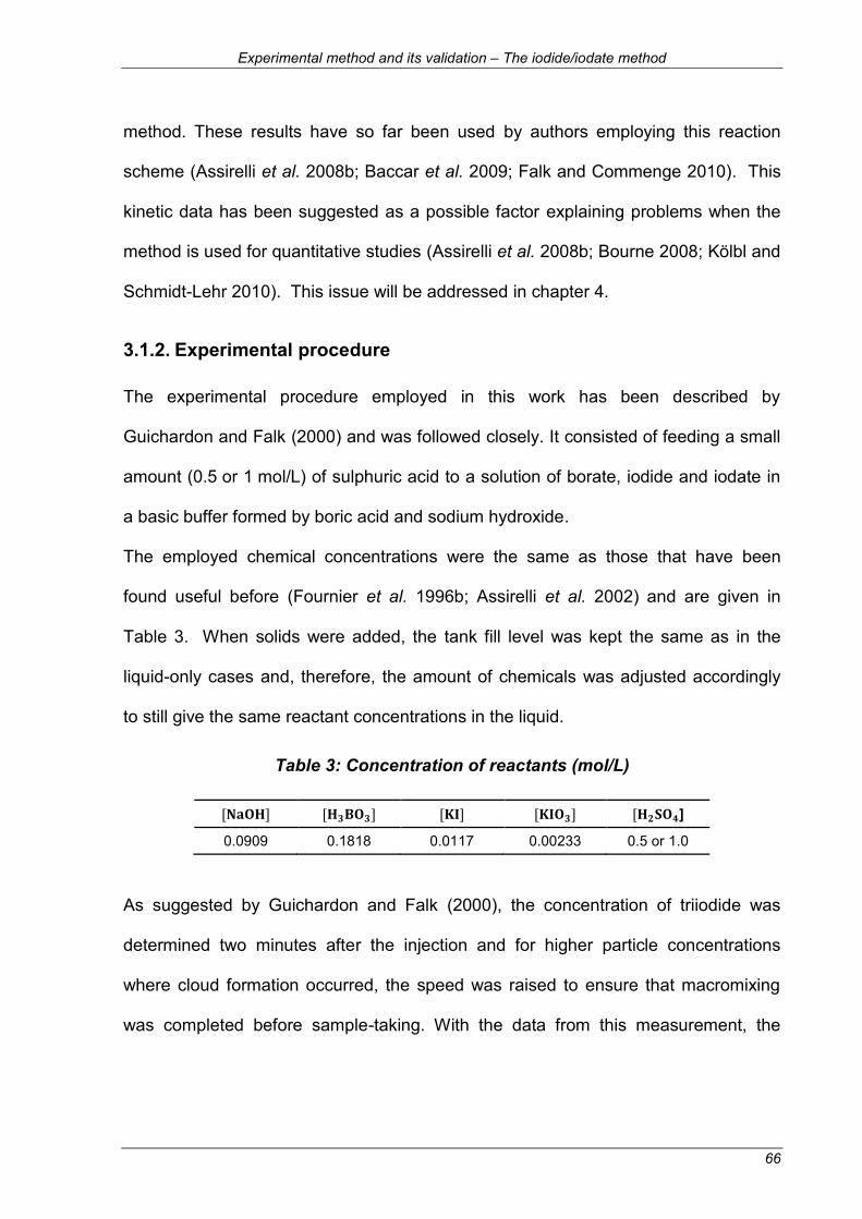
Experimental method and its validation – The iodide/iodate method
66
method. These results have so far been used by authors employing this reaction
scheme (Assirelli et al. 2008b; Baccar et al. 2009; Falk and Commenge 2010). This
kinetic data has been suggested as a possible factor explaining problems when the
method is used for quantitative studies (Assirelli et al. 2008b; Bourne 2008; Kölbl and
Schmidt-Lehr 2010). This issue will be addressed in chapter 4.
3.1.2. Experimental procedure
The experimental procedure employed in this work has been described by
Guichardon and Falk (2000) and was followed closely. It consisted of feeding a small
amount (0.5 or 1 mol/L) of sulphuric acid to a solution of borate, iodide and iodate in
a basic buffer formed by boric acid and sodium hydroxide.
The employed chemical concentrations were the same as those that have been
found useful before (Fournier et al. 1996b; Assirelli et al. 2002) and are given in
Table 3. When solids were added, the tank fill level was kept the same as in the
liquid-only cases and, therefore, the amount of chemicals was adjusted accordingly
to still give the same reactant concentrations in the liquid.
Table 3: Concentration of reactants (mol/L)
]
0.0909 0.1818 0.0117 0.00233 0.5 or 1.0
As suggested by Guichardon and Falk (2000), the concentration of triiodide was
determined two minutes after the injection and for higher particle concentrations
where cloud formation occurred, the speed was raised to ensure that macromixing
was completed before sample-taking. With the data from this measurement, the

Experimental method and its validation – The iodide/iodate method
67
segregation index or selectivity for side-product, XS, can be calculated which is used
to quantify micromixing efficiency:
(3.4)
It is defined as the ratio of actual yield of unwanted product, Y, to the maximum yield
at total segregation, YST. Therefore, the segregation index can range from 0 to 1 with
in the case of perfect micromixing and for total segregation.
For these reactions, the yield is calculated as:
(3.5)
In the case of total segregation, both reactions are quasi-instantaneous compared to
micromixing time and consequently stochiometry determines the amount of side-
product:
(3.6)
Another way of quantifying micromixing, as described by Villermaux and David
(1983), is the micromixedness ratio, . The idea is that the flow consists of regions
which are either perfectly mixed or fully segregated. From this concept, has been
defined as the ratio of the volumes of perfectly mixed (PM) to totally segregated (ST)
fluid. It can be easily calculated from the segregation index which is well-defined for
these cases (PM: ST: ) (Fournier et al. 1996b; Guichardon and Falk
2000):

Experimental method and its validation – Experimental set-up
68
(3.7)
The values of the micromixedness ratio might be more intuitive to use for some, as
micromixing effectiveness improves with increasing .
An advantage of the iodide/iodate technique, compared to other reaction-based
methods, is that more than one injection can be done per experiment, which reduces
waste, time and cost. The segregation index is then calculated taking the previous
injections and samplings into account as described in literature (Guichardon and Falk
2000; Assirelli 2004).
For the two-and three-phase results, in addition to the “normal”, i.e. single-phase,
definition of the segregation index itself, it was found in this work useful to plot data as
the deviation of XS, in %, from the corresponding reference, e.g. single-phase, results:
(3.8)
This way of expressing changes in the segregation index has also been employed in
this context by other authors (Unadkat 2009).
3.2. Experimental set-up
3.2.1. The rig
For the experimental part of this work, a cylindrical Perspex vessel with a flat bottom
and a diameter of 288 mm was employed. It was surrounded by a square water
jacket which allowed distortion-free viewing and helped keeping the temperature in
the tank constant. In addition, the vessel contained four equally-spaced baffles
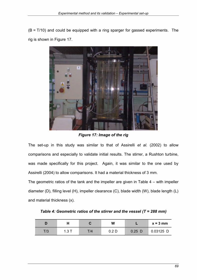
Experimental method and its validation – Experimental set-up
69
(B = T/10) and could be equipped with a ring sparger for gassed experiments. The
rig is shown in Figure 17.
Figure 17: Image of the rig
The set-up in this study was similar to that of Assirelli et al. (2002) to allow
comparisons and especially to validate initial results. The stirrer, a Rushton turbine,
was made specifically for this project. Again, it was similar to the one used by
Assirelli (2004) to allow comparisons. It had a material thickness of 3 mm.
The geometric ratios of the tank and the impeller are given in Table 4 – with impeller
diameter (D), filling level (H), impeller clearance (C), blade width (W), blade length (L)
and material thickness (x).
Table 4: Geometric ratios of the stirrer and the vessel (T = 288 mm)
D H C W L x = 3 mm
T/3 1.3 T T/4 0.2 D 0.25 D 0.03125 D

Experimental method and its validation – Experimental set-up
70
The fill level and the impeller clearance were chosen to avoid air entrainment from
the liquid surface (Assirelli 2004).
The power input from the impeller could be measured with a strain gauge on the
shaft combined with telemetry. Such measurements are well-established and have
been described in literature (Bujalski et al. 1987; Ascanio et al. 2004). Initial liquid-
only tests were performed to check the power number of the Rushton turbine used.
Table 5 shows these results compared against literature and good agreement was
found; the match is especially close with Assirelli et al. (2002), who used a very
similar system.
Table 5: Power number in liquid-only system – compared to literature
Water height this work reference
H=T 4.20 4.61 Bujalski et al. (1987)
H=1.3H 4.35 4.33 Assirelli et al. (2002)

Experimental method and its validation – Experimental set-up
71
3.2.2. Adaptions for the reaction system
The reactant, in these experiments, sulphuric acid, could be fed with glass pipes
which had inner diameters of 0.8 to 1 mm at the tip. The glass pipes were stabilised
by steel pipes and fixed from the sides and top of the vessel. This allowed accurate
positioning and re-positioning – even when the pipes had to be taken out of the
system, for instance for cleaning or repairs. A steady flow was ensured by employing
a peristaltic pump with two pump heads which were out of phase. Such a set-up was
chosen because Assirelli (2004) reported pulsation from a pump with less rollers than
the one employed in the actual study.
Figure 18 shows the employed locations for feeding sulphuric acid and Table 6 gives
the coordinates. The choice of the feed positions was based on current knowledge
from single-phase experiments: considering that significant differences in
micromixing quality between feeding near the surface and closer to the impeller are
now well-established, a position in the impeller discharge stream and another one
close to the surface were chosen, similar to Assirelli et al. (2002). It must be
emphasised that these locations are similar, but not exactly equivalent due to
technical differences in the rigs employed. Moreover, studies on turbulence
modulation in stirred tanks have indicated that turbulence might be most significantly
spatially affected near . Therefore, position 4 in this study is equivalent to
position 4 in Assirelli et al. (2002), though the difficulty of accurate positioning of feed
pipes still needs to be remembered – especially, in the light of the significant changes
of energy dissipation near the impeller. In addition, feed position 3, at a height
halfway between vessel bottom and impeller, was employed for some single-phase

Experimental method and its validation – Experimental set-up
72
and further sparged experiments to give a better picture of the effect of bubbles on
micromixing.
Figure 18: Schematic of mixing tank and feed positions
Table 6: Coordinates of the feed positions
2r/D z/H
position 1 2.24 0.92
position 2 2.19 0.27
position 3 2.24 0.096
position 4 1.06 0.22
3.2.3. Sample taking and measurement of triiodide
Samples could be taken from a pipe with a tap at the side of the vessel. This pipe
and tap were repositioned to check independence of sampling position. As expected
for a well (macro-)mixed tank, the location of sample taking did not have any

Experimental method and its validation – Validation of method - single-phase results
73
influence on the micromixing results. Obviously, the dead volume in the pipe was
always removed before actual samples were taken.
Each measured value actually consists of the average of the reading from three
samples in separate cuvettes, to avoid errors.
The concentration of triiodide was determined using a single-beam
spectrophotometer (Cecil CE 1020) at 353 nm, which is one of the two peaks in the
spectrum of triiodide and iodine (Awtrey and Connick 1951). Guichardon and Falk
(2000) illustrated that the extinction factor of triiodide varies for different
spectrophotometers. Therefore, a calibration curve was obtained, following the
procedure described by Assirelli (2004), for the employed apparatus. This gave an
extinction coefficient of 2560.8 m2/mol at 353 nm which is in very good agreement
with literature (Guichardon and Falk 2000; Assirelli 2004). Details of the calibration
and a comparison to values from literature can be found in Appendix A.
3.3. Validation of method - single-phase results
The method is validated in this section by repeating similar experiments those in
literature. In addition, this data will give a baseline for comparison of the results of
the 2- and 3-phase studies.
3.3.1. Meso-/micromixing transition
Initial experiments had the purpose of finding feed rates suitable for micromixing
studies, i.e. lower than mesomixing dominated while still avoiding backmixing.
Assirelli (2004) found a range of 1-3 ml/min useful in a similar stirred vessel. Figure
19 gives a similar result and a feed rate of 2 ml/min was chosen for all experiments
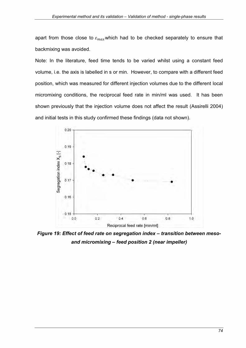
Experimental method and its validation – Validation of method - single-phase results
74
apart from those close to which had to be checked separately to ensure that
backmixing was avoided.
Note: In the literature, feed time tends to be varied whilst using a constant feed
volume, i.e. the axis is labelled in s or min. However, to compare with a different feed
position, which was measured for different injection volumes due to the different local
micromixing conditions, the reciprocal feed rate in min/ml was used. It has been
shown previously that the injection volume does not affect the result (Assirelli 2004)
and initial tests in this study confirmed these findings (data not shown).
Figure 19: Effect of feed rate on segregation index – transition between meso-
and micromixing – feed position 2 (near impeller)

Experimental method and its validation – Validation of method - single-phase results
75
Figure 20: Effect of feed rate on segregation index – transition between meso-
and micromixing – feed position 4 (near )
Figure 20 illustrates that the effect of the tested feed rates near is relatively
small compared to Figure 19, but, in order to avoid backmixing, a higher rate of
3 ml/min was chosen. Moreover, higher amounts of sulphuric acid were fed per
injection at this position due to good micromixing which led to low iodine yields.
Consequently, the increased feed rate also helped keeping the duration of the
experiments within a reasonable range.
3.3.2. Single-phase – comparison to literature
Figure 21 presents micromixing results as a function of mean specific power input
obtained for three feed positions and these are compared to literature (Assirelli
2004). In the current work, the range of impeller speeds was also extended to higher
values mainly, to allow possibly complete particle suspension in corresponding solid-
liquid experiments.

Experimental method and its validation – Validation of method - single-phase results
76
Figure 21: Segregation indices at 3 feed positions as a function of mean power
input – compared to results from similar experiments (Assirelli 2004)
In spite of the slightly different feed points (they deviated by about 0.5 and 1 cm
radially for position 1 near the surface and 2 near the impeller respectively from the
equivalent position in the earlier work), the data (Figure 21) agrees very well with the
results of Assirelli (2004). In two tanks and impellers designed to be identical with
exactly the same feed rates and compositions and the same range of specific power
inputs, Assirelli (2004) observed differences in of between 8% and 14% and the
current results were all within 14% of the previous ones.
The excellent agreement at position 4, near , is especially remarkable as this
region could be expected to show particular sensitivity to positioning due to the
strong gradients of local energy dissipation rates (Assirelli et al. 2002).

Experimental method and its validation – Validation of method - single-phase results
77
It can be concluded that the single-phase experiments are in good agreement with
earlier ones, which gives confidence in the method and the set-up. Therefore, the
results are suitable as a baseline for comparing with the data obtained in the
presence of the second phase and also for testing the micromixing modelling.

Incorporation model: adaptation and its use to interpret experimental data – Introduction
78
4. INCORPORATION MODEL: ADAPTATION AND ITS USE
TO INTERPRET EXPERIMENTAL DATA
4.1. Introduction
Though the iodide/iodate method has been widely used, recently, its usefulness as a
means of obtaining quantitative data about the local turbulence has been questioned
(Bourne 2008; Kölbl and Schmidt-Lehr 2010) because the reaction kinetics are not
sufficiently well understood, as discussed in further detail in section 2.2.3.
Especially, the dissociation of sulphuric acid, which supplies the limiting reactant, ,
needs attention. Nevertheless, this method has been found to give qualitatively
reliable results (Bourne 2008), while being easier to use than other reaction schemes
(Aubin et al. 2010) and versatile, especially, as this method allows adapting the
reactant concentrations to give maximum sensitivity for micromixing in a specific case
(Guichardon and Falk 2000). In order to address the issues found in recent
literature, micromixing modelling might be of use, as calculating an independent
value, like a micromixing time, e.g. the reciprocal value of the Engulfment rate
(Baldyga and Bourne 1999) or the incorporation time (Villermaux and Falk 1994),
might allow comparing results obtained from different reactant concentrations.
Taking into account that such models have been found useful in various systems
(Baldyga and Bourne 1989a; Baldyga and Bourne 1989b), such an approach is worth
further evaluation. Before the mentioned criticism was published and could have
been considered, such work had already been done with the Iodide/iodate method to
estimate energy dissipation levels in a stirred tank using the incorporation model
Incorporation model: adaptation and its use to interpret experimental data – Introduction
79
(Assirelli et al. 2008b). Unfortunately, the results were only in reasonable agreement
with comparable data from other methods.
The incorporation model will also be employed here, as it has been attacked less and
taking into account that a similar model, the Engulfment model, has given realistic
results for stirred tanks when validated against experimental data (Bourne and Yu
1994). Therefore, further work on such an approach seems warranted. In addition,
its advantages are that it is relatively simple (Fournier et al. 1996a) and
computationally not too expensive, especially when solved with efficient algorithms
as suggested by Assirelli et al. (2008b).
The incorporation model follows the changes of the species’ concentrations in a
small volume of feed solution while it grows due to incorporation, as described in
section 2.2.3. For a given characteristic time, micromixing time, this model then
allows calculating the product distribution of chemical test reactions which are
sensitive to micromixing, in this case the iodide/iodate method. Therefore, a
connection between an experimentally obtained segregation index and is given.
This micromixing time then allows estimating the local specific energy dissipation rate
“experienced” by the chemical reactants via 1/E (Baldyga and Bourne 1990) or
(Fournier et al. 1996a):
(4.1)
Unfortunately, the existing approach for the Iodide/iodate reaction scheme does not
reflect too well what is actually expected to occur during such studies. New
variations are presented here: the model is extended to include the partial

Incorporation model: adaptation and its use to interpret experimental data – Materials and method
80
dissociation of sulphuric acid and different kinetic rate laws are tested. These
modelling results are then applied by interpreting experimental data from a single-
phase stirred tank, for instance to estimate local specific energy dissipation rates.
Comparisons of these results to literature might help selecting the (currently) most
suitable approach and could give ideas for further studies.
4.2. Materials and method
4.2.1. Adapted model for the iodide/iodate method
As discussed in section 2.2.3., Kölbl and Schmidt-Lehr (2010) demonstrated that
is not fully dissociated when being fed into a stirred tank and, therefore, not all
protons are immediately available for the reaction, which had been assumed in most
previous work. As a solution, the authors proposed using a stronger acid, e.g.
perchloric acid, or considering the second dissociation of sulphuric acid when using a
micromixing model. The latter option has also been suggested by Bourne (2008) in a
critical discussion of the iodide/iodate method. Therefore, the current approach
(Fournier et al. 1996a) is first briefly explained and then extended to include the
dissociation of the sulphuric acid.
In the incorporation model, the changes of the reactant concentrations in an
aggregate or blob of feed solution are observed: as described in section 2.2.3., the
concentrations of the species j in the reaction zone are given by considering the
balance of incorporation and chemical reaction (with subscript 10 indicating the
concentration in the surrounding liquid):

Incorporation model: adaptation and its use to interpret experimental data – Materials and method
81
(4.2)
The reaction volume grows over time due to incorporation of surrounding fluid, i.e.
. This behaviour has been tested for instance for linear and
exponential growth rates (Assirelli et al. 2008b), with the latter being the better
established one (Zwietering 1984; Baldyga and Bourne 1999; Assirelli et al. 2008b):
(4.3)
A mole balance following equation (4.2) can then be formulated for each of the
species as described by Fournier et al. (1996a). This was given in a dimensionless
form using Damköhler numbers and by normalising against , the initial
concentration of protons in the injection volume, assuming full dissociation, and ,
for the reactants and for time, respectively. The species were then represented by :
(4.4)
With the initial conditions:
,
The balances for the species can then be summarised (Fournier et al. 1996a;
Assirelli et al. 2008b) as:
(4.5)
(4.6)
(4.7)
(4.8)

Incorporation model: adaptation and its use to interpret experimental data – Materials and method
82
(4.9)
with (c’ refers to concentration before mixing):
,
,
,
and:
,
,
where:
,
,
This approach was presented by Fournier et al. (1996a). For this work, some
changes to the mole balances and additional values are needed for and
to calculate their change during the dilution. Of course, the initial values for ,
and depend on the concentration of sulphuric acid before the injection
and would be the respective concentration at equilibrium divided by the initial proton
concentration. However, as the assumption of a known, well-defined
is not valid,
the dimensionless expressions were changed in the approach used here from the
original to , the initial amount of iodate in the bulk:
(4.10)
Consequently, the Damköhler numbers and become:
(4.11)
(4.12)
And in the incorporation terms in the dimensionless form for the species are:

Incorporation model: adaptation and its use to interpret experimental data – Materials and method
83
,
,
These alterations from normalising against initial H+-concentration to initial iodate
concentration in the bulk should not affect the final results of the incorporation model
as long as it is being done consistently. The results are validated in section 4.3.
The main adaptation here, compared to Fournier et al. (1996a), is to include the
second dissociation of sulphuric acid. This was fairly straight-forward: the relevant
dimensionless concentrations were converted back to absolute concentrations, the
change in the equilibrium due to the dilution calculated and then the respective slope
returned to the solver algorithm, here Runge-Kutta. This allows calculation of the
dissociation at each time step.
Technical note: The equilibrium changes due to dilution are, however, always
calculated ahead for the next time step as the change in concentrations will only
effectively be “available” to the reactions in that next step. This formulation was
chosen, as it might be argued that the effect of dilution and dissociation is
instantaneous compared to the other reactions. Therefore, this effect should
immediately become relevant in the current time step. In spite of being, if neglected,
only a small delay, it was considered accordingly.
Regardless of such details, the calculation of the dilution requires a constant (or, at
least, known) time step size which reduces the options of accelerating the code, for
instance with adaptive time steps.

Incorporation model: adaptation and its use to interpret experimental data – Materials and method
84
4.2.2. Kinetics
Kinetics for the current approach
So far, the approach presented by Fournier et al. (1996a), which employs kinetic data
for the Dushman reaction, equation (3.2), measured by the same research group
(Guichardon et al. 2000), has been used for modelling the Iodide/iodate reaction
scheme. They gave the reaction rate as a function of ionic strength:
for the classic 5th order behaviour which has been found by many workers before
(see the papers by Guichardon et al. 2000; Bourne 2008):
In the kinetic study by Guichardon et al. (2000), sulphuric acid was used and the
authors assumed that it was fully dissociated. This might not, like in the actual
experimental procedure, be valid at the employed concentrations, especially
considering the use of to adjust the ionic strength, which has also been found
problematic in recent measurements (Kölbl and Hecht 2012). Consequently, the
concentration of in the original model seems to be in doubt.
For this extended incorporation model, the question of using appropriate kinetic data
needs to be addressed again because the dissociation of the acid will be added and
this might be an (even) less than ideal combination with the original approach. Other
options can at least be considered, particularly, as it has been suggested that the
incorporation model is very sensitive to kinetics (Villermaux and Falk 1994) and as
such data is available and has not been tested in such an approach before.

Incorporation model: adaptation and its use to interpret experimental data – Materials and method
85
Options for employing alternative kinetics
To discuss the kinetics in more detail, the reactions are summarised again:
(4.13)
(4.14)
(4.15)
While reactions (4.13) and (4.15) are kinetically well defined and have not been
criticized in this context, reaction (4.14) is more problematic, in spite of significant
research efforts. More than a century ago, Dushman (1904) was the first author who
suggested a rate law for this reaction which is now known as the Dushman reaction.
Nevertheless, its kinetics are still being discussed in literature (Schmitz 1999; Xie et
al. 1999; Agreda B. et al. 2000; Schmitz 2000; Bourne 2008; Kölbl 2008; Kölbl et al.
2011). Thus, this section gives a brief review of the most appropriate data and also
mentions some problems with the measurements in the kinetic studies.
Some of the difficulties encountered in earlier work may be explained by the results
of Barton and Wright (1968): They found in their experiments that species present in
buffers can have an effect on the Dushman reaction by causing catalysis by
carboxylate and phosphate ions. The authors proposed a reaction rate of
(4.16)
where is for the investigated buffer species. The authors found, for five bases
studied, that the catalytic rate constant kb follows Brönsted law with
even though Bamford and Tipper (1972) showed changes of up to 30% of the
observed rate due to catalysis. This illustrates that it could be necessary to consider

Incorporation model: adaptation and its use to interpret experimental data – Materials and method
86
also the effect of additional species which are present in the solution during the
experiments. For instance, in the case of the iodide/iodate reaction scheme, the
effect of the borate ions has not been investigated.
Liebhafsky and Roe (1979) concluded a paper on this reaction emphasising the
computer’s value when a mechanism, not the mechanism, is the only realistic goal.
This might not sound exceedingly encouraging for solving the difficulties with this
reaction, but some of the authors’ suggestions were considered in later work by
Palmer and Lyons (1988). In that case, stopped-flow spectrophotometry was used to
study the Dushman reaction at three ionic strengths, with variation of iodide and
perchloric acid concentrations, at several temperatures. Palmer and Lyons (1988)
found, as have many other authors (Guichardon et al. 2000; Bourne 2008), 5th order
kinetics and dependence on ionic strength. Table 7 gives their rate constants, which
the authors also found to be in good agreement with previous work.
Table 7 : Rate constants of Dushman reaction for three ionic strengths by Palmer and Lyons (1988)
I [M] k [M-4s-1]
0.015 6.72 · 108
0.10 4.27 · 108
1.00 2.62 · 108
Schmitz (1999) reviewed issues found in literature, like the effect of the buffer and
changes in the order of iodide, i.e. from 1 to 2 and then less than 2, with increasing
concentrations of that reactant. Starting from this point, the author described a
kinetic mechanism which accounts for the effects mentioned above, like the buffer’s

Incorporation model: adaptation and its use to interpret experimental data – Materials and method
87
influence. Unfortunately, there is still significant uncertainty regarding the coefficients
of the resulting kinetic model, as also admitted by the author. For this reason, the
model suggested by Schmitz (1999) is not employed in this work.
Xie et al. (1999) measured kinetics in a special device, which is suitable for fast
reactions, at relatively high iodide but low iodate concentrations and also showed
saturation effects at higher reactant concentrations. Therefore, the following
expression, which leads to lower orders for and than with the established
classic 5th order law, was given:
(4.17)
Without such saturation, the rate constant would be at an ionic
strength of 0.5 M (Xie et al. 1999). A similar study (Agreda B. et al. 2000) using a
stopped-flow apparatus found such saturation effects at higher concentrations too.
The authors suggested that the ratio has been found relevant, but in their
study , which is not comparable to conditions found when using the
Iodide/iodate method.
Schmitz (2000) soon afterwards showed new data and argued that the above two
publications (Xie et al. 1999; Agreda B. et al. 2000) support previously presented
ideas (Schmitz 1999). Schmitz’s measurements (2000) covered, both, the first and
the second order behaviour of iodide. Unfortunately, the conditions, especially the
low iodide concentrations and the ratio , were far from being comparable to
those for the iodide/iodate reaction scheme, which might not be ideal for application
to the conditions typically used in micromixing studies. A rate law was proposed in
this study for an ionic strength of 0.2 M:

Incorporation model: adaptation and its use to interpret experimental data – Materials and method
88
(4.18)
All the experiments leading to the above kinetic information were performed at much
lower concentrations than would be present in the iodide/iodate measurements
during micromixing studies, in particular in stirred tanks. Considering that changes in
reaction order have been observed over a range of reactant concentrations, applying
these rate laws could be problematic. It might be argued that the rate-determining
step changes for such different conditions (Bourne 2008). In addition, buffers and
various ions have been shown to affect the reaction. Therefore, a more targeted
investigation should be considered for this case.
In addition to the above full kinetic rate laws, Kölbl et al. (2011) recently presented
new reaction orders for the Dushman reaction which were measured at higher
concentrations and with borate, which should give more useful data for using the
Iodide/iodate method in stirred tanks than previous studies. Unfortunately, to date
the authors have not found a full expression which would include a kinetic constant.
Nevertheless, this new interest in the reaction gives hope for moving the reaction
scheme towards a more quantitatively reliable method. Kölbl et al. (2011) proposed
the following orders at conditions relevant to micromixing studies in stirred tanks:
(4.19)
As no other or more suitable data is available at this point, several of the above rate
laws are tested.

Incorporation model: adaptation and its use to interpret experimental data – Materials and method
89
Possible indications from studies on reverse reactions
As mentioned earlier in this section, the effect of borate on the Dushman reaction is
not known. However, results from studies on related processes might give some
indication: other phenomena in this context like the reverse reaction and reaction
steps for instance the disproportionation of iodine in basic media or related species
like hypoiodous acid, respectively, have been investigated in several studies, too.
Motivation behind such work was for instance in the context of nuclear plant
accidents, clock reactions or regarding drinking and sea water (Bichsel and von
Gunten 2000; Sebodblack-Nagy and Körtvélyesi 2004; Buxton and Mulazzani 2007;
Schmitz 2008).
It has been shown that the disproportionation of hypoiodous acid may be catalysed
by buffers containing phosphate, borate, or acetate, but inhibited by ammonia (by 50-
80%) (Bichsel and von Gunten 2000). In fact, the behaviour with added species has
been found to be complex and might not be easily described for a wide range of
conditions (Truesdale et al. 2003). As mentioned above, catalysis of the Dushman
reaction due to carboxylate and phosphate ions has also been reported (Barton and
Wright 1968), but the effect of borates is not known and there is not as much
information on buffer species as in the reverse cases. Therefore, a brief look at such
literature might give some indication of appropriate directions for future work or even
help with improving the modelling in the current work.
In addition to changes in rate-limiting reaction steps due to the different reactant
concentrations or “an” interaction of borate and/or boric acid and the reacting species
being an option in general, specific effects might be hypothesised. Such effects may
Incorporation model: adaptation and its use to interpret experimental data – Materials and method
90
be suggested from literature, for instance between borate and HIO, which has been
repeatedly mentioned as an intermediate in the Dushman reaction (Schmitz 1999;
Xie et al. 1999). It was even suggested as part of the potentially rate-determining
step (Barton and Wright 1968). In addition, as would be expected, also other
intermediates which have been proposed for the mechanisms can be found for both
reactions (Urbansky et al. 1997). Considering that borate has already been shown to
catalyse the disproportionation of hypoiodous acid for some time (Buxton and Sellers
1985; Truesdale 1995), it might be conceivable that such phenomena could slow
down the Dushman reaction under the conditions of the Iodide/iodate reactions
scheme – i.e. the intermediate product, HIO, would not only react to iodine but to an
increased extent follow the catalysed disproportionation back to iodide and iodate
due to the presence of borate. Clearly, these are just ideas and need experimental
investigation.
Interestingly, also unusual behaviour has been shown: among the few studies into
buffer effects, it has been found that acetate can both catalyse and suppress the
disproportionation of hypoiodous acid (Urbansky et al. 1997). This is remarkable for
the iodide/iodate method as such opposing phenomena might precipitate unexpected
additional complexities into an already challenging reaction system. Though, taking
the consistent qualitative data from micromixing experiments into account, there is
hope that the overall effect of borate might be less difficult to handle here.
Again, it has to be emphasised that the above is only speculative as also other steps
of the reaction might be affected and the overall effect cannot be adequately
estimated, let alone calculated, without suitable data from a targeted experimental
study – which, unfortunately, is not within the scope of this work. Therefore,
Incorporation model: adaptation and its use to interpret experimental data – Materials and method
91
regardless of the conclusions here, a study investigating the Dushman reaction under
conditions similar to those in the Iodide/iodate reaction scheme is needed.
Nevertheless, also trends in the modelling results from employing the kinetics
discussed above might give some indication of what kinetics would have to be
expected when taking evidence from the extensive amount of data on mixing
experiments into account.
From the literature above, an “informed guess” of the effect of borate might be a
reduction in reaction rate. From the changes reported and considering the
concentrations in the reacting volume in micromixing experiments in stirred tanks, it
might be estimated that the reaction could be slowed down to half or a quarter of the
unaffected kinetics. Therefore, a third of k (from possibly suitable and reliable
uncatalysed kinetic data) might be tested as an additional option, if the rate laws
above fail to give more realistic results than the current model. It can be argued that
such effects could depend on the concentration of borate, which changes throughout
the micromixing process and consequently would have to be considered, if this is
indeed the critical species. However, Truesdale et al. (2003) found that such buffer
interactions also depend on the iodide concentration, which, again, changes
throughout the process. Consequently, the above variation seems to be the most
reasonable estimate possible at this point, i.e. as long as there is no further
information on the specific conditions.
4.2.3. Numerical method
Guichardon (1996) used the fourth-order Runge-Kutta method to solve the
incorporation model for the iodide/iodate reaction scheme, while Assirelli et al.
(2008b) employed Bader and Deuflhard's semi-implicit discretisation in the Bulirsch-

Incorporation model: adaptation and its use to interpret experimental data – Materials and method
92
Stoer method. The latter approach is more complex, but is computationally more
efficient and especially suitable for stiff equations. Assirelli et al. (2008b) neglected
the effect of the reactions on the ionic strength in the Jacobian matrix, which was
justified because it changes slowly and only has a small effect compared to other
parameters. Both methods give, as expected, very similar results (Assirelli 2004),
further justifying both ways of solving the model.
In this study, the fourth-order Runge-Kutta method was chosen because of its
simplicity which allows quick adaptation of the code to different kinetic models, in
spite of being less efficient compared to the second option. Moreover, calculating the
dissociation of sulphuric acid ahead of the next time step, as discussed above
(see section 4.2.1), was less problematic to implement with this method with defined
time steps.
The code was written in C and is based on the information given in literature
(Fournier et al. 1996a; Assirelli 2004).
4.2.4. Polynomial regression for quantitative comparison
Micromixing experiments, as described in section 3.1.2., give results as segregation
index, , or micromixing ratio, , for specific experiments, i.e. particular fluid
dynamic conditions and reactant concentrations. Micromixing models calculate the
final reactant concentrations – and consequently give or – from given values of
micromixing time. The results from the models are then usually plotted in graphical
form with (or ) as a function of micromixing time. In order to make use of these
results, functions tend to be fitted to the modelling data which then allows
micromixing times to be obtained for each experimental condition.

Incorporation model: adaptation and its use to interpret experimental data – Results and discussion
93
In this work, polynomial regression was chosen for this quantitative comparison as
suggested by Assirelli et al. (2008b). The equation used is:
with y = ln( ) and x = ln( ).
Other authors (Camps Rota 1998; Rousseaux et al. 1999) reported fitting different
functions to separate parts of the data, which would be an option if polynomial
regression does not work sufficiently well. The validity and accuracy of employing
this function was checked for all results with .
4.3. Results and discussion
4.3.1. Validation of the implemented model
There are two options for testing the code: firstly, the results of the model without the
dilution routine should still give the same results as those found in the literature.
Figure 22 shows the result from the approach in this work, as outlined in section 4.1.,
and compares the predictions to those of Guichardon (1996) and Assirelli (2004). As
can be seen, excellent agreement is obtained. Any small differences between the
predictions are probably due to different numerical approaches (Assirelli 2004).

Incorporation model: adaptation and its use to interpret experimental data – Results and discussion
94
Figure 22: Comparison of the implemented routine to equivalent results from
the literature (Assirelli 2004)
Due to the close agreement between the three predictions shown in Figure 22, the
earlier values for three different sulphuric acid concentrations taken from Assirelli et
al. (2008b) were used for further validation of the code. Again, Figure 23 shows
excellent agreement. Still, as these graphs are plotted over a wide range of values
for and tm on logarithmic axes, smaller differences might not be apparent.
Therefore, also polynomial regression was employed and a comparison of 3 points
for each group of curves confirms that the method is working, as only deviations of
less than 0.5% were found (data not shown).
tm [s]
0.0001 0.001 0.01 0.1 1
[-]
1
10
100
this workAssirelli (2004)Guichardon (1996)

Incorporation model: adaptation and its use to interpret experimental data – Results and discussion
95
Figure 23 : Comparison of results from the present model with those of
Assirelli et al. (2008b) at 3 acid concentrations
In addition to validating the results of the model with fully dissociated sulphuric acid,
the dilution of the latter can be checked separately as well, i.e. without the other
reactions occurring. The data presented in Figure 24 is obtained from simple
equilibrium calculations using Excel spreadsheet for several concentrations and
equivalent cases when using the model. The results clearly agree well. Moreover,
there is an overlap of the concentrations of and at the dilution of 2 M by
250; this is exactly at the concentration suggested by Leenson (2004).
tm [s]
0.0001 0.001 0.01 0.1 1
[-]
1
10
100
0.5 M this work1.0 M this work2.0 M this work
tm [s]
0.0001 0.001 0.01 0.1 1
[-]
1
10
100
0.5 M Assirelli (2004)1.0 M Assirelli (2004)2.0 M Assirelli (2004)
tm [s]
0.0001 0.001 0.01 0.1 1
[-]
1
10
100
0.5 M Assirelli (2004)1.0 M Assirelli (2004)2.0 M Assirelli (2004)

Incorporation model: adaptation and its use to interpret experimental data – Results and discussion
96
Figure 24: Species concentrations after dilution without reactions occurring
A comparison of all data points to the manually calculated values showed excellent
agreement with the worst deviation being -0.012%, which is to be expected due to
rounding errors.
4.3.2. Modelling results and use for interpreting experimental data
Established model and implemented dissociation
After testing the code, the combination of the original kinetics with implemented
dilution and dissociation of the sulphuric acid was evaluated. This first combination
might be considered to be mainly for demonstration purposes as this kinetic data was
obtained assuming that all protons are already initially available.

Incorporation model: adaptation and its use to interpret experimental data – Results and discussion
97
Figure 25: Incorporation model with initially fully dissociated sulphuric acid
and with dilution implemented – kinetic data: Guichardon et al. (2000)
Figure 25 shows the results for the model with implemented dilution of the acid
compared to the original data. There is a significant shift of the curves on the log-log-
graph when dilution of the acid is implemented. Considering Assirelli et al. (2008b)
found that the original model allowed at least reasonably realistic interpretation of
experimental data, this large change may indicate that the original kinetic data might
not be suitable in this case with dilution. This can be tested by comparing the
variations for actual experimental data. Therefore, the micromixing times for the
segregation indices are calculated from regression of the model results, as discussed
above. These values are then put into equation (4.1) to estimate and . The
results at different power inputs for feeding near , the impeller and the surface
are summarised in Table 8, Table 9 and Table 10, respectively.

Incorporation model: adaptation and its use to interpret experimental data – Results and discussion
98
Table 8: Comparison of assuming full dissociation or including dissociation in model for position 4 (near ) – using kinetics from Guichardon et al. (2000)
fully dissociated acid partial dissociation of acid
[W/kg] [W/kg] [-] [W/kg] [-]
0.18 24.143 134.129 2.008 11.158
0.50 53.958 107.915 5.118 10.235
0.97 63.406 65.367 6.148 6.338
1.94 81.481 42.000 8.145 4.199
Table 9: Comparison of assuming full dissociation or including dissociation in model for pos. 2 (near impeller) – using kinetics from Guichardon et al. (2000)
fully dissociated acid partial dissociation of acid
[W/kg] [W/kg] [-] [W/kg] [-]
0.18 0.978 5.434 0.043 0.239
0.40 1.752 4.379 0.087 0.216
0.50 2.147 4.294 0.110 0.221
0.97 3.492 3.600 0.198 0.204
1.14 3.649 3.201 0.209 0.183
Table 10: Comparison of assuming full dissociation or including dissociation in model for pos. 1 (near surface) – using kinetics from Guichardon et al. (2000)
fully dissociated acid partial dissociation of acid
[W/kg] [W/kg] [-] [W/kg] [-]
0.18 0.053 0.293 0.001 0.008
0.40 0.110 0.275 0.003 0.008
0.50 0.136 0.273 0.004 0.008
0.97 0.246 0.253 0.008 0.009
1.14 0.261 0.229 0.009 0.008

Incorporation model: adaptation and its use to interpret experimental data – Results and discussion
99
Of course, increases with increasing power input, which is correctly reflected in the
above tables. On the other hand, the obtained decreased with impeller speed,
especially closer to the impeller, which is found with both versions of the model.
Literature indicates that this value should be relatively independent of impeller speed
in each location, for instance: LDV data for a Rushton turbine reported by Zhou and
Kresta (1996) fluctuated by less than 2.5 % over the range from 225 to 510 rpm
when expressed as . Effects of the impeller speed, however, have already
been found previously in micromixing experiments (Baldyga and Bourne 1999;
Assirelli et al. 2008b). It can be argued that either the path of the reaction becomes
shorter due to better (micro)mixing at higher impeller speeds, giving more localised
information, or that the reactants might be swept away more quickly into regions of
different energy dissipation rate, which could lead to the observed effect. The above
trends point more towards the latter explanation because there are reductions of XS
which are stronger near the impeller, i.e. there is a substantial drop to 49% of from
0.18 to 0.97 W/kg near , but only a drop to 87% near the surface. For this
reason, most of the following considerations will discuss lower impeller speed –
assuming that having a possibly localised reaction zone allows sensible comparisons
to local energy dissipation rates reported in literature. It should be noted, though,
that such significant changes might be explained partially by a less than suitable
micromixing model.
Measurements of local specific energy dissipation rates have been done with a range
of methods: values from ~20 (Sharp and Adrian 2001)(PIV) or 25 (Wu and Patterson
1989), 35 (Laufhütte and Mersmann 1987)(LDA) to ~70 (Cutter 1966), using a
photographic technique, have been found for , which is close to the impeller. In

Incorporation model: adaptation and its use to interpret experimental data – Results and discussion
100
the bulk and in particular towards the surface, much lower values have been
observed for , i.e. around and well below 1. Such wide ranges of potentially
realistic for different locations in the tank are clearly far from ideal for the validation
of a model and the difficulties of the various laser-based methods for obtaining such
values have also been illustrated (Micheletti et al. 2004; Gabriele et al. 2009). Still,
there is enough data from detailed and careful studies using modern techniques
which can aid verifying that the results are in a realistic order of magnitude. For this
purpose, the most reasonable estimates seem to be around 50 near (Zhou and
Kresta 1996; Schäfer 2001), around or slightly less than 1 for the feed position in the
impeller discharge stream but away from the impeller and well below 1 near the
surface.
A comparison of this literature to the results in Table 8, Table 9 and Table 10 shows
that the original model consistently gives higher values than expected while including
the dissociation of sulphuric acid leads to rather low ones. Clearly, both versions are
not giving the expected results, but are still within a reasonable range. Further
testing of variations of the model seems warranted.
Considering dissociation – combined with other kinetics from literature
Using the implemented dissociation with other kinetic data might give more realistic
results and some of the investigated options are summarised here.
One interesting kinetic rate law, as proposed by Schmitz (2000), shows first and
second order behaviour of iodide and could be relevant because it might cover a
wide range of conditions. Unfortunately, the concentrations of iodide were still very
low in that study and this might render the data less useful in this context considering
recent criticism (Bourne 2008). Nevertheless, it seemed interesting to test.

Incorporation model: adaptation and its use to interpret experimental data – Results and discussion
101
Figure 26: Results for original model (fully dissociated) – compared to: with
dilution implemented using kinetic data by Schmitz (2000)
Figure 26 shows that the curves are closer to the original model than the same
version with dilution. Nevertheless, there are deviations especially towards very high
and lower micromixing times because the new curves are less steep than the original
ones. The resulting values of and do not give more realistic results than the
original approach. Especially, near is significantly higher instead of giving a
lower value as would be expected:
Table 11: Results for model considering dissociation of acid using kinetics from Schmitz (2000) – at different feed positions at 0.18 W/kg
feed position [W/kg] [-]
1 – near surface 0.038 0.213
2 – near impeller 1.505 8.360
4 – near 97.668 542.598

Incorporation model: adaptation and its use to interpret experimental data – Results and discussion
102
Another option would be the kinetic data reported by Palmer and Lyons (1988). As
they gave rates for three different ionic strengths, the one for I = 1M was first tested.
Figure 27 shows that the graphs are, again, less steep than the previously reported
ones and, overall, in spite of the different measurement approaches, resemble the
result for the kinetics reported by Schmitz (2000) - see Figure 26.
Figure 27: Results for original model (fully dissociated) – compared to: with
dilution implemented using kinetic data by Palmer and Lyons (1988) for I = 1M
Table 12: Results for model considering dissociation of acid using kinetics from Palmer and Lyons (1988) for I = 1M – at different feed positions at 0.18 W/kg
feed position [W/kg] [-]
1 – near surface 0.047 0.260
2 – near impeller 1.79 9.93
4 – near 103 573
Table 12 shows that the values of are surprisingly close to the ones in Table 11
and they are still worse, i.e. further away from expected for these values, than the
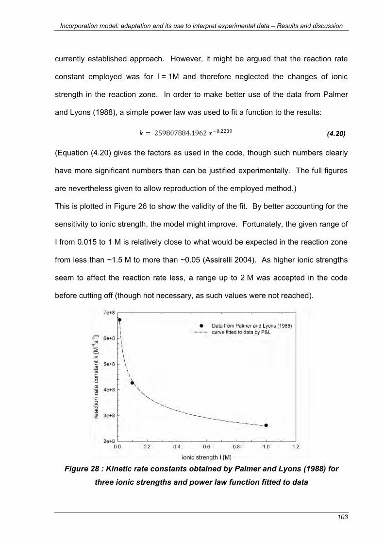
Incorporation model: adaptation and its use to interpret experimental data – Results and discussion
103
currently established approach. However, it might be argued that the reaction rate
constant employed was for I = 1M and therefore neglected the changes of ionic
strength in the reaction zone. In order to make better use of the data from Palmer
and Lyons (1988), a simple power law was used to fit a function to the results:
(4.20)
(Equation (4.20) gives the factors as used in the code, though such numbers clearly
have more significant numbers than can be justified experimentally. The full figures
are nevertheless given to allow reproduction of the employed method.)
This is plotted in Figure 26 to show the validity of the fit. By better accounting for the
sensitivity to ionic strength, the model might improve. Fortunately, the given range of
I from 0.015 to 1 M is relatively close to what would be expected in the reaction zone
from less than ~1.5 M to more than ~0.05 (Assirelli 2004). As higher ionic strengths
seem to affect the reaction rate less, a range up to 2 M was accepted in the code
before cutting off (though not necessary, as such values were not reached).
Figure 28 : Kinetic rate constants obtained by Palmer and Lyons (1988) for
three ionic strengths and power law function fitted to data

Incorporation model: adaptation and its use to interpret experimental data – Results and discussion
104
Figure 29: Results for original model (fully dissociated) – compared to: with
dilution implemented using interpolated function of kinetic data by Palmer and Lyons (1988)
This interpolation does indeed move the results slightly closer towards what would be
expected for , as illustrated in Table 13. Nevertheless, this still does not give more
realistic values than the original, heavily criticised method.
Table 13: Results for model considering dissociation of acid using data from Palmer and Lyons (1988) interpolated function for I – at different feed positions
at 0.18 W/kg
feed position [W/kg] [-]
1 – near surface 0.035 0.197
2 – near impeller 1.32 7.34
4 – near 76.7 426.4
Another study with relevant kinetic data was presented by Xie et al.(1999) who used
a special method which is particularly suitable for studying such fast reactions. The

Incorporation model: adaptation and its use to interpret experimental data – Results and discussion
105
kinetics may be employed, as described above, in full with dependence on saturation
or as a constant. Both options were tested and gave very similar results. Therefore,
the constant value (for I=0.5 M) was used for detailed evaluation and Figure 30
shows that this also resembles the above trends.
Figure 30: Results for original model (fully dissociated) – compared to: with
dilution implemented using kinetic data by Xie et al. (1999)
Table 14: Results for model considering dissociation of acid using data from Xie et al. (1999) – at different feed positions at 0.18 W/kg
feed position [W/kg] [-]
1 – near surface 0.017 0.093
2 – near impeller 0.685 3.803
4 – near 41.399 229.995
In this case, the values for lie between the original and the other adaptations’ but
also do not move much closer to improving the method for interpreting experimental

Incorporation model: adaptation and its use to interpret experimental data – Results and discussion
106
data obtained by the Iodide/iodate method. However, all of these results are
surprisingly consistent which is remarkable when taking the different measurement
methods into account and that even the relatively unrelated data by Schmitz (2000)
points towards a similar direction. This would not have been expected, considering
the many, but valid, points of criticism (Bourne 2008).
To further emphasise the agreement of these kinetics: it was even possible to
combine the data by Palmer and Lyons (1988) and Xie et al. (1999) in one
interpolated function. This equation (4.21) is very similar to (4.20) and should not
affect the results reported above too much, but was still tested for completeness:
(4.21)
(Again, level of detail only to allow exact reproduction of data!)
The agreement of the (little) available (relatively) suitable data is illustrated in Figure
31 which also shows the functions fitted to the kinetic constants.
Figure 31: Kinetic rate constants obtained by Palmer and Lyons (1988) and Xie et al. (1999) for different ionic strengths and power law function fitted to data
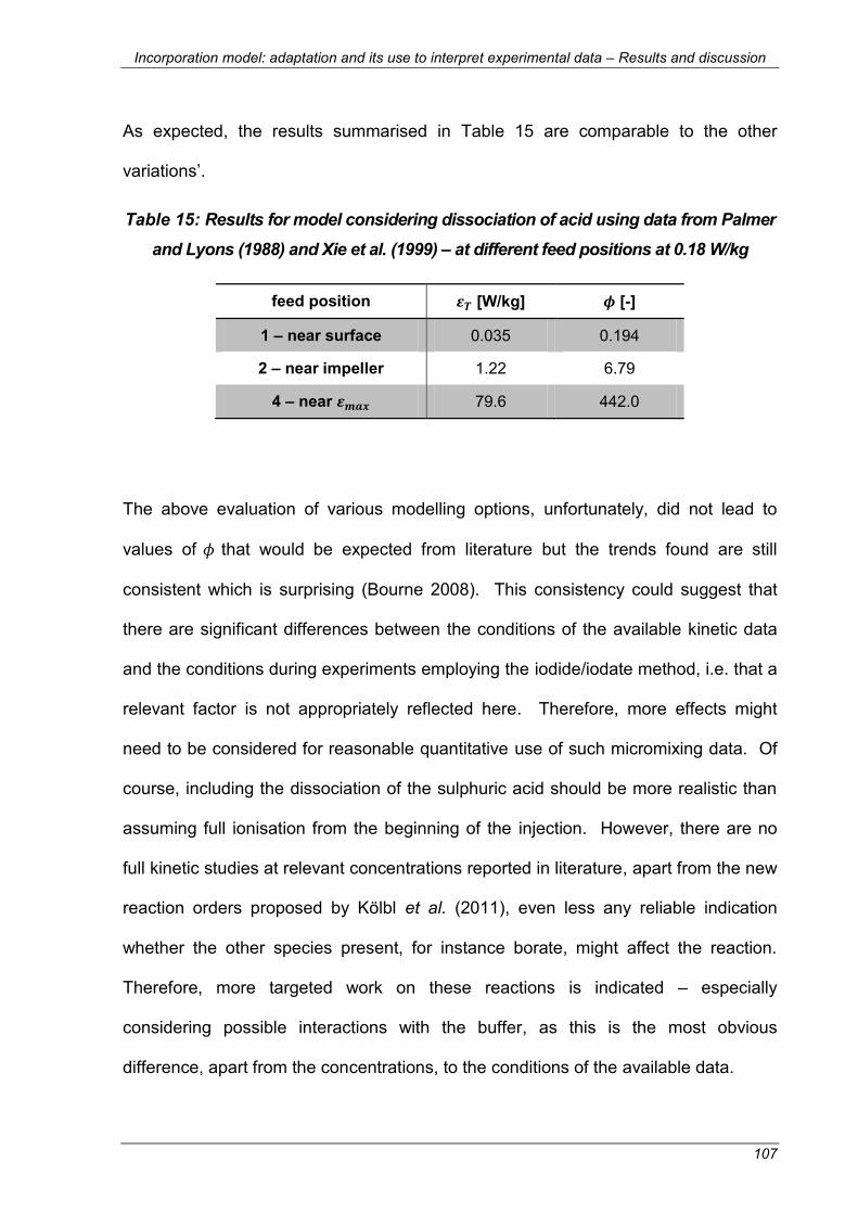
Incorporation model: adaptation and its use to interpret experimental data – Results and discussion
107
As expected, the results summarised in Table 15 are comparable to the other
variations’.
Table 15: Results for model considering dissociation of acid using data from Palmer and Lyons (1988) and Xie et al. (1999) – at different feed positions at 0.18 W/kg
feed position [W/kg] [-]
1 – near surface 0.035 0.194
2 – near impeller 1.22 6.79
4 – near 79.6 442.0
The above evaluation of various modelling options, unfortunately, did not lead to
values of that would be expected from literature but the trends found are still
consistent which is surprising (Bourne 2008). This consistency could suggest that
there are significant differences between the conditions of the available kinetic data
and the conditions during experiments employing the iodide/iodate method, i.e. that a
relevant factor is not appropriately reflected here. Therefore, more effects might
need to be considered for reasonable quantitative use of such micromixing data. Of
course, including the dissociation of the sulphuric acid should be more realistic than
assuming full ionisation from the beginning of the injection. However, there are no
full kinetic studies at relevant concentrations reported in literature, apart from the new
reaction orders proposed by Kölbl et al. (2011), even less any reliable indication
whether the other species present, for instance borate, might affect the reaction.
Therefore, more targeted work on these reactions is indicated – especially
considering possible interactions with the buffer, as this is the most obvious
difference, apart from the concentrations, to the conditions of the available data.

Incorporation model: adaptation and its use to interpret experimental data – Results and discussion
108
4.3.3. Including dissociation and adapted kinetic model
Due to the effects of borate on the reverse reaction and reaction steps discussed in
section 4.2.2., it could be argued that the reaction might be slowed down significantly in
the presence of the buffer. The above modelling results also suggest a slower side-
reaction and therefore, that option had to be considered too. This is especially true due
to the excellent agreement of the data from uncatalysed and not inhibiting systems. The
data from the most sophisticated methods (Palmer and Lyons 1988; Xie et al. 1999)
agreed well and, consequently, the interpolated function (4.21) was used for this
purpose. The initial estimate, for order of magnitude, was a reduction, as explained in
section 4.2.2., to a third of the unaffected reaction rate and, therefore: kadapted=k(4.19)/3.
Figure 32: Results for original model (fully dissociated) – compared to:
included dissociation and adapted kinetic behaviour
The trend of the curves in Figure 32 looks different from the previous ones, as they
are above the original ones, while again being less steep. Of course, application to
experimental data is necessary for quantification. Therefore, a range of power inputs
for three feed positions are evaluated and summarised here:

Incorporation model: adaptation and its use to interpret experimental data – Results and discussion
109
Table 16: Comparison of original model and new approach including dissociation and using adapted kinetics - for position 4 (near )
fully dissociated acid partial dissociation of acid
[W/kg] [W/kg] [-] [W/kg] [-]
0.18 24.14 134.13 8.04 44.69
0.50 53.96 107.92 21.10 42.21
0.97 63.41 65.37 25.50 26.29
1.94 81.48 42.00 34.11 17.58
Table 17: Comparison of original model and new approach including dissociation and using adapted kinetics - for position 2 (near impeller)
fully dissociated acid partial dissociation of acid
[W/kg] [W/kg] [-] [W/kg] [-]
0.18 0.978 5.434 0.146 0.809
0.40 1.752 4.379 0.304 0.761
0.50 2.147 4.294 0.394 0.787
0.97 3.492 3.600 0.727 0.749
1.14 3.649 3.201 0.768 0.674
Table 18: Comparison of original model and new approach including dissociation and using adapted kinetics - for position 1 (near surface)
fully dissociated acid partial dissociation of acid
[W/kg] [W/kg] [-] [W/kg] [-]
0.18 0.053 0.293 0.004 0.020
0.40 0.110 0.275 0.009 0.023
0.50 0.136 0.273 0.012 0.024
0.97 0.246 0.253 0.025 0.026
1.14 0.261 0.229 0.027 0.024

Incorporation model: adaptation and its use to interpret experimental data – Results and discussion
110
The results of for the adapted version are, for the conditions in a stirred tank, much
closer to what would be expected, even though the effect of the buffer is assumed to
be constant, i.e. 1/3 of k. There could, however, be a concentration dependence
which would be difficult to estimate due to the complex behaviour reported for other
species (Truesdale 1997). Consequently, this is mainly for illustration purposes, but
can be easily changed once suitable experimental data is available.
In addition it could be noted, that the original kinetics by Guichardon et al. (2000) give
reasonable results and show strong dependence on ionic strength. Their observation
of dropping reaction rate with increasing ionic strength might be explained by their
use of to adapt ionic strength, which then reduced the amount of available .
In fact, their rate constant changes by orders of magnitude with ionic strength: from
109 to 107 from 0 to 1.4 M, respectively. Such dramatic effects were not
observed by Palmer and Lyons (1988). Considering that the buffer significantly
contributes to the ionic strength, an inhibiting effect of borate might have been
“accidentally included” and, therefore, explain the reasonable results when
interpreting stirred tank experiments. In addition, iodide concentration, which has
been shown to shift such effects (Truesdale et al. 2003), also depends on
incorporation to which ionic strength is correlated. Therefore, the kinetics reported by
Guichardon et al. (2000) might also indirectly account for such phenomena.
This also supports the assumption of an inhibited reaction, but further data is needed.

Incorporation model: adaptation and its use to interpret experimental data – Results and discussion
111
4.3.4. Use of such models to compare data
At same reactant concentrations – with varied flow conditions
Such modelling results might not only be of use for giving absolute information on
local turbulence. Also, comparisons of results for different flow conditions would be
useful. Therefore, the single-phase data presented above (section 3.2.3.) is
expressed here once as Φ in Table 19, which shows the strong variations of the data.
However, when given as percent of reference values at different feed positions, as
illustrated in Table 20, the data becomes much more consistent – even for the wide
range of values tested, i.e. from the highest to the lowest local specific energy
dissipation rates in the stirred tank. This suggests that, although the kinetics and the
effect of the buffer need further consideration, comparisons of experimental results
are possible at least with same reactant concentrations in the stirred tank.
Table 19: Summary of Φ at various locations at 0.18 W/kg – shows significant differences, but consistent pattern in data
model near near impeller near surface
original 134 5.43 0.293
original + diss. 11 0.24 0.008
Schmitz 543 8.36 0.213
Palmer and Lyons (1M) 573 9.93 0.260
P&L (interpolated) 426 7.34 0.197
Xie et al. 230 3.80 0.093
P&L+Xie (interpolated) 442 6.79 0.194
adapted 45 0.80 0.020

Incorporation model: adaptation and its use to interpret experimental data – Results and discussion
112
Table 20: Relative comparisons of Φ in % of various locations at 0.18 W/kg – data becomes more consistent than in Table 19
model impeller to surface to surface to impeller
original 4.05% 0.218% 5.39%
original + diss. 2.14% 0.068% 3.17%
Schmitz 1.54% 0.039% 2.55%
Palmer and Lyons (1M) 1.73% 0.045% 2.62%
P&L (interpolated) 1.72% 0.046% 2.68%
Xie et al. 1.65% 0.040% 2.44%
P&L+Xie (interpolated) 1.54% 0.044% 2.86%
adapted 1.78% 0.045% 2.51%
This agreement of the data in Table 20 suggests that these model variations can be
used for comparisons, though the absolute values (Table 19) vary significantly.
At same flow conditions– with varied reactant concentrations
Besides testing the models at different feed positions, different acid concentrations
might be used as well. In this case, the segregation indices are not the same at
equal conditions, as the reactions are affected by the reactant concentrations.
Therefore, the micromixing model should then give comparable micromixing times
and local specific energy dissipation rates, i.e. the results should then overlap within
experimental error.
Such tests have already been done before (Assirelli 2004; Assirelli et al. 2008b). In
that work, the original modelling approach was used and good agreement of the data
for different acid concentrations was found once the results were presented as
micromixing times or local specific energy dissipation rates, instead of or . The

Incorporation model: adaptation and its use to interpret experimental data – Results and discussion
113
model variations tested above will, therefore, be applied to the experimental data by
Assirelli (2004). This might help evaluate the suitability of the employed kinetics.
For feed position 3, Assirelli (2004) reported micromixedness ratios for two acid
concentrations ( = 1 and 2 M) at four impeller speeds. With the original
micromixing model a standard deviation around 20% for is found between the data
for the two acid concentrations for the four power inputs. The adapted versions give
slightly worse agreement with standard deviations around 27% for . However,
experimental errors are also magnified in such calculations and can reach over 30%
for in the given data set, even when only the reported experimental error is
considered. In addition to this, there might also be differences in micromixing itself,
as changes in acid concentrations might lead to differently long trajectories before
the last has reacted and therefore different local conditions experienced –
similarly to the deviations with changing impeller speeds. Assirelli (2004) used =
1 and 4 M to study micromixing near the impeller and found backmixing effects for
the higher acid concentration at higher impeller speed. This finding also supports the
above argument about inherent differences with varied acid concentrations, which
can (and should) not be compensated for by the model, as they indeed are real
effects in the flow. Therefore, a comparison of the data near – where such
phenomena might be especially likely – is not of use for evaluating the model
variations.
Unfortunately, no further data is available for such comparisons, but the above does
not suggest significant differences in the suitability of the different adaptations and
the more established original version.

Incorporation model: adaptation and its use to interpret experimental data – Conclusions
114
4.4. Conclusions
The current approach of the iodide/iodate method, which assumes fully dissociated
sulphuric acid, has been criticised in literature and, consequently, the incorporation
model, which has been used for this reaction scheme before, was extended
accordingly. In addition, different kinetics were implemented to find a variation that
gives more realistic values of than the existing modelling – with a focus on stirred
tanks.
The results from employing different rate laws for the Dushman reaction were
surprisingly consistent, but gave higher than would be expected from mixing
literature. As the effect of the buffer is not well understood in this case, information
on the possible interaction of borate with the reverse reaction of the Dushman
reaction and related reactions was discussed. From these considerations, the effect
of borate on the reaction scheme was estimated. This lead to more realistic results,
but further work in this direction is needed. Recently, the potential difficulties
encountered with such measurements, even in modern apparatuses, were discussed
(Kölbl 2008). Nevertheless such data is urgently needed to develop the iodide/iodate
method from a qualitatively reliable to a quantitatively sound technique to study
micromixing processes in a variety of geometries.
Until such data becomes available, the previously reported model and above
approach should be suitable, at least, for comparing experimental results relative to
each other and for order of magnitude estimates of local energy dissipation rates or
in stirred tanks. Therefore, in this thesis, data will be interpreted using the original
model and some variations, as presented in this chapter.

Micromixing in gas-liquid systems – Introduction
115
5. MICROMIXING IN GAS-LIQUID SYSTEMS
5.1. Introduction
A dispersed, gaseous phase, i.e. bubbles, is present in many mixing applications
using stirred tanks, including those where micromixing is important, for instance
fluorination or hydrogenation. The effect of gas bubbles on micromixing in agitated
vessels is not very well characterised, see section 2.3.3., and this chapter is aimed at
giving a clearer picture of whether and, if so, how significantly gas sparging affects
micromixing in them. For this purpose, three feed positions were investigated under
gassed conditions: near the surface (pos 1), near the impeller (pos 2) and below the
impeller (pos 3) – see Figure 18.
In this chapter, first the method is validated for gas-liquid studies, then experimental
conditions defined and results from these experiments reported. In addition, these
will be discussed using the modelling described in the previous section.
5.2. Validation of the experimental method for sparged conditions
To use the iodide/iodate technique in gassed systems, the chemicals and their
reactions should only be affected by the sparging of the gas due to changes in
micromixing, not by any undesired reactions, either physical or chemical. Therefore,
it was necessary to check that the method would not fail in these conditions.
5.2.1. Loss due to gas stripping
One question was whether the gassing process might strip any reactants from the
liquid which would cause misleading results. Especially iodine, which is produced

Micromixing in gas-liquid systems – Validation of the experimental method for sparged conditions
116
during the experiments, needs to be considered because of the substance’s high
volatility.
Several solutions containing all reactants including iodine and triiodide at various
concentrations and different pH-values which would be present in typical experiments
were sparged with air and samples taken over time. The triiodide concentration from
these experiments was compared to samples of the solution taken from the vessel
before sparging.
Figure 33: An example of the effect, with time, of air sparging at 1.0 vvm on the
absorbance, i.e. triiodide concentration, of a typical solution of reactants
A typical set of data from these tests is plotted in Figure 33 and allows observation of
any stripping effects for the duration of the planned experiments. Even after 35
minutes of aeration, deviations of less than ±1.5% between the triiodide
concentration in the sparged vessel and the unsparged reference solution were

Micromixing in gas-liquid systems – Power input in sparged cases
117
observed. This is in agreement with Lin and Lee (1997) who did not find any losses
either, even at their higher sparge rates of up to 10 vvm.
5.2.2. Oxidation of iodide
Another concern which has been mentioned previously by some authors (Lin and
Lee 1997; Schäfer 2001) is the oxidation of iodide:
(5.1)
Due to this Lin and Lee (1997) used nitrogen instead of air and also prepared the
solutions with continuous N2 stripping in order to avoid any oxidation of reactants.
Considering that this oxidation can only take place when H+ is available and is
relatively slow (Harris 1995), it can be expected that it would not be relevant in the
bulk of the stirred liquid which has to have a higher pH for these studies anyway.
Sparging iodide/iodine solutions in a pH-range from the expected basic conditions to
neutral with nitrogen or air did not show any deviations in behaviour in triiodide
concentration, which was expected for the above reasons.
Consequently, the gassed experiments could be performed using air.
5.3. Power input in sparged cases
5.3.1. Power measurement results in gas-liquid cases
As discussed in section 2.1.3., the power input of Rushton turbines can be
significantly affected by the sparging of gas. In order to investigate the effect of the
added phase on micromixing, the impeller speed had to be adapted to give constant
impeller power input. For this, power measurements of the gassed system were
performed. Considering the well-established fact that some salts can affect

Micromixing in gas-liquid systems – Power input in sparged cases
118
coalescence (Lessard and Zieminski 1971; Craig et al. 1993), all experiments were
conducted using the actual solutions and the resulting power curves are plotted in
Figure 34 – as relative power demand against gas flow number.
Figure 34: Relative power demand as function of gas flow number – gassed
Figure 34 generally shows the typical power behaviour of Rushton turbines in
sparged systems, i.e. dropping with increasing gassing rates. However, the minimum
at cannot be seen because these parts of the power inputs were outside of the
measurement range of the torque meter. Still, for all three gassing rates, the points
of flooding were captured, which could also be observed visually during the
experiments, though the absolute values of power input in this lower range will be
different. The lower values of the measured power were, unfortunately, out of range
for technical reasons (these parts of the graphs are in a faint colour) and

Micromixing in gas-liquid systems – Power input in sparged cases
119
consequently could not be used for determining constant mean specific power input
in the micromixing experiments. For all results below 0.4 W/kg, the measurement
was considered to not be accurate enough for the intended purpose and only values
above that level have been used. Nevertheless, the overall trends look as expected
compared to literature (Harnby et al. 1997). In addition, also the power
measurements in the single-phase case agree well with literature which shows that
the data in the range above 0.4 W/kg should be reliable.
5.3.2. Conditions for micromixing experiments with gas
For the above reasons, the following impeller speeds were employed to keep the
power input from the impeller constant:
Table 21: Impeller speeds at several gassing rates for matching mean specific energy dissipation rates
[W/kg]
0.0 vvm [rpm]
0.5 vvm [rpm]
1.0 vvm [rpm]
1.5 vvm [rpm]
0.18 300
0.40 395 495 535 569
0.50 420 527 567 607
0.97 522 638 682 745
1.14 552 670 721 781
5.3.3. Flow at the chosen conditions
At all of these conditions for the micromixing experiments, even at the lowest power
input and highest gassing rate, the impeller was not flooded, which could be
observed visually and from the power data which is summarised in section 5.3.1. At

Micromixing in gas-liquid systems – Micromixing near impeller under gassed conditions
120
such, conditions, when the gas is dispersed in the tank, it would usually not be
possible to see the feed pipe during the experiments. However, Assirelli (2004)
recommended leaving a small gas bubble at the tip of the feed pipe before starting
the injection to keep the fluids from interacting too early which was found useful in
this work as well. The start of the injection would then start when that little bubble
has left the pipe which can be seen clearly in single-phase experiments with glass
pipes. For many multi-phase cases shown here this was not possible, but the “dead
time” was checked during test runs and could therefore easily be considered in the
actual experiments.
Sometimes the amount of gas sparged is expressed as superficial gas velocities.
For completeness, these are given in Table 22 – note that in this case the aspect
ratio of the tank is 1.3.
Table 22: Superficial gas velocities
gas rate [vvm] superficial gas velocity [m/s]
0.5 0.00312
1 0.00624
1.5 0.00936
5.4. Micromixing near impeller under gassed conditions
Figure 35 shows the segregation index as a function of impeller power input for two
gassing rates, 0.5 and 1.0 vvm, and corresponding single-phase data for
comparison. Only broad conclusions can be drawn from this graph, as the
segregation index is slightly higher in some of the gassed cases, but these deviations

Micromixing in gas-liquid systems – Micromixing near impeller under gassed conditions
121
might be negligible, considering the error bars. In addition, one might expect
stronger effects with increasing gassing rates, which is not the case in these results.
Figure 35 does indicate, however, that any possible effects on micromixing due to the
presence of gas bubbles can be expected to be small or negligible near the impeller
at constant energy input.
Although it has been shown in the previous section that power data below 0.4 W/kg
is not reliable enough for being used in the main part of this study, some tests were
done at the lowest power input, 0.18 W/kg, and 0.5 vvm. Interestingly, the
segregation index is lower than under “comparable” single-phase conditions. This
might be due to the underestimated power number of the gassed impeller which
leads to higher impeller speeds than actually needed, i.e. higher power input into the
system and therefore improved micromixing.
Another explanation might be the ratio of power put into the system due to gassing
compared to stirring: it may be argued that the power input from the impeller is low
enough in this case to actually have a noticeable effect of the power put into the
system from the gas sparging, which would be relatively small at the higher power
inputs. The power input from the gas is discussed in part 5.8.
Obtaining more reliable power data would be necessary to allow comparisons in that
range, but technical limitations did not permit this at lower power inputs.
Consequently, only conditions with accurately measured power inputs, as described
above, are considered in the further investigation – which still leaves a useful range
of power inputs which are relevant to industry.

Micromixing in gas-liquid systems – Micromixing near impeller under gassed conditions
122
Figure 35: as a function of mean specific energy dissipation rate at various
gassing rates – impeller feed with 1 mol/L
As the set of results from the experiments with 1 mol/L sulphuric acid is rather limited
in number of data points and does not show any systematic trends due to sparging,
further runs were done with 0.5 mol/L which is expected to give higher sensitivity to
micromixing. This improvement is due to the different relative changes in reaction
rates with varying acid concentration and has already before been used for adapting
the method to specific measurement problems (Guichardon and Falk 2000; Assirelli
2004; Kölbl et al. 2008).

Micromixing in gas-liquid systems – Micromixing near impeller under gassed conditions
123
Figure 36: as a function of mean specific energy dissipation at varied
gassing rates – impeller feed with 0.5 mol/L
Figure 36 illustrates the effect of gassing on the segregation index dependent on the
impeller power input – as shown in Figure 35, but here for a different acid
concentration (0.5 mol/L) and up to 1.5 vvm gassing rate. As in the previous figure,
there is no significant deviation or systematic trend due to gassing: the values are
relatively close to the single-phase results, i.e. with overlapping error bars, and there
is no consistent pattern with increasing gassing rate. At the lowest investigated
power input, i.e. 0.4 W/kg, a small improvement of micromixing efficiency could be
suspected due to the consistent, though small, deviation from the unsparged value.
This might be explained, as mentioned above, by the higher relative impact of the
power input from the gas compared to the impeller.

Micromixing in gas-liquid systems – Micromixing near impeller under gassed conditions
124
Overall, Figure 36 nevertheless shows that micromixing near the impeller under
gassed conditions is mainly affected by the impeller power input, at least for the
conditions investigated. The deviations from the single-phase result can be
explained with experimental error of the micromixing experiments themselves and
also with errors from the power measurements.
Figure 37: Influence of aeration rate on segregation index at several levels of mean specific energy dissipation rate as percentage of single-phase results –
impeller feed with 0.5 mol/L
Figure 37 compares the data to the single-phase reference as , which magnifies
any effects from Figure 36. The graph confirms that the deviations of the gassed
experiments from the liquid-only cases at equivalent power inputs from the impeller
are small, i.e. not more than 7% and usually less than ±5% of the segregation index
deviation, which is within the expected and observed ranges of error.

Micromixing in gas-liquid systems – Micromixing near impeller under gassed conditions
125
An alternative criterion to mean specific power input might be impeller tip speed or
impeller speed. Figure 38 gives an impression of the data’s correlation with impeller
speed. Clearly, the data does not correlate as well as with and .
Figure 38: as a function of impeller speed at varied gassing rates – impeller
feed with 0.5 mol/L
From the above results, it can be suggested that the impeller is the dominating factor
for specific energy dissipation rates and, linked to it, micromixing in this region of the
agitated vessel. Consequently, any contribution to or effect on micromixing due to
the gas is negligible at the conditions investigated. A similar conclusion was drawn
by Bourne (1994) referring to data from a PhD thesis (Hilber 1987) employing a
Bourne reaction. Interestingly, Brilman et al. (1999) used diazo-coupling and only
reported very little effect of gassing when feeding near the impeller or about halfway

Micromixing in gas-liquid systems – Micromixing near free surface under gassed conditions
126
between impeller and surface. This would, of course, still be in agreement with this
work, but the authors kept the impeller speed constant in their work. Therefore, it is
expected that the mean energy dissipation due to agitation was not constant,
especially as a six-bladed “Rushton-like” (Brilman et al. 1999) turbine was used. At
least for the lower gassing rates in their work, i.e. about 0.5 and 1.0 vvm, this cannot
be explained. At their highest gassing rate, the system might have been flooded,
which may lead to different results.
In addition to directly contributing to the energy dissipated, the bubbles might also
lead to turbulence modulation. Considering the wide range of bubble sizes found in
stirred tanks (Barigou and Greaves 1992), it would be difficult, if at all possible, to
estimate an overall effect. The results for the feed position in the impeller discharge
stream, however, do not indicate turbulence modulation.
In order to get a better impression of micromixing in a sparged stirred vessel, further
feed positions were studied.
5.5. Micromixing near free surface under gassed conditions
The results for the same experimental conditions when feeding near the free surface
are shown in Figure 39. In contrast to the results for the impeller region, the
segregation index significantly drops with increasing aeration rate. Moreover, while
at 0.5 vvm some dependence on mean specific power input from the impeller might
still be seen, micromixing seems to become dominated and, in fact, determined by
gas sparging.

Micromixing in gas-liquid systems – Micromixing near free surface under gassed conditions
127
Figure 39: as a function of mean impeller specific energy dissipation rate at
different gassing rates – surface feed with 0.5 mol/L
The improvements of for feeding near the surface as seen in Figure 39 are
dramatic: the segregation index drops at 0.5 W/kg from 0.23 without gas to 0.16 with
1.5 vvm. This is comparable to values measured in the impeller discharge stream,
e.g. 0.14 at 0.5 W/kg.
In order to quantify that improved micromixing, the deviation of the gassed
segregation indices from the single-phase data is plotted in percent against the
gassing rate in Figure 40. This graph shows improvements of up to 30% in terms of
segregation index. Furthermore, the similar improvements, regardless of power
input, clearly illustrate the significant effect of the gassing rate on micromixing
efficiency.

Micromixing in gas-liquid systems – Micromixing near free surface under gassed conditions
128
Figure 40: Reduction of segregation index compared to the unsparged value at
several mean specific energy dissipation rates – surface feed with 0.5 mol/L
Figure 41: as a function of impeller speed at different gassing rates –
surface feed with 0.5 mol/L

Micromixing in gas-liquid systems – Micromixing below impeller under gassed conditions
129
Figure 39 and Figure 40 indicate that the power input from the impeller becomes less
relevant with increasing gassing rates. This is emphasised in Figure 41 which shows
that the segregation index does not correlate any better with impeller speed than with
mean specific energy dissipation rate. Sparging seems to be the critical factor.
5.6. Micromixing below impeller under gassed conditions
As gas sparging dramatically improves micromixing near the surface, but shows no
significant effects near the impeller for the investigated conditions, an additional feed
position (3) below the stirrer was studied. Figure 42 gives an overview of the results
for feeding below the impeller. As expected, the segregation indices of the
unsparged reference data are slightly higher – about 10% in – than the ones from
feeding into the impeller discharge stream (previous section, 5.5.). In addition, the
errors are slightly larger below the impeller, i.e. from 1-2% at position 2 to 3-4% at
position 3.
These gassed results do not show a clear trend with increasing sparge rate and
fluctuate near the single phase values. At most conditions, the error bars overlap
and a consistent effect is not obvious from Figure 42, though the data for most
gassed cases, especially 1 vvm, is slightly lower than the single-phase equivalents.
This might indicate that there is a small contribution from the gas power input
towards the local specific energy dissipation rates, which might be more relevant in
this region of the tank where the absolute value of ε is expected to be lower than in
position 2, but higher than in position 1 – which is confirmed by the single-phase
micromixing data. Another explanation for the fluctuations could be that the flow
below the impeller might change slightly between the various conditions even though

Micromixing in gas-liquid systems – Micromixing below impeller under gassed conditions
130
the impeller was always loaded. Errors in the measurements of the impeller’s power
input do not seem responsible for the deviations in Figure 42 as the same impeller
speeds were set for the experiments at position 2 which, however, do not lead to
comparable trends.
Figure 42: as a function of mean specific energy dissipation at varied
gassing rates – feed below impeller with 0.5 mol/L
In order to emphasise and clarify any effects in the sparged experiments, the results
are plotted in Figure 43 as deviation from the reference single-phase data. Again,
the slight improvements of up to 5-10% of the segregation index, in particular at
1 vvm, can be seen. It may be argued that, at least at the lowest power input, an
effect of the gassing rate is indicated, but, overall, it is not possible to draw clear
conclusions from the available data.

Micromixing in gas-liquid systems – Micromixing below impeller under gassed conditions
131
Figure 43: Influence of aeration rate on segregation index at several levels of mean specific energy dissipation rate as percentage of single-phase results –
feed below impeller with 0.5 mol/L
Considering the proximity to the stirrer, an effect of the impeller speed or impeller tip
speed (in contrast to mean specific power input) might be another option. Therefore,
the results are plotted against N in Figure 44. Although the experiments were not
laid out for comparable impeller speeds, they are within a similar range and allow a
reasonable plot. Unfortunately, the graph does not indicate any better correlation
with N than with .

Micromixing in gas-liquid systems – Micromixing under gassed conditions without power input from impeller
132
Figure 44: as a function of impeller speed at varied gassing rates – feed
below impeller with 0.5 mol/L
5.7. Micromixing under gassed conditions without power input
from impeller
Some micromixing experiments were done with the impeller not being switched on to
investigate the effect of the gas bubbles without any further power inputs. Figure 45
shows the segregation indices as a function of sparge rate for feeding near the
surface and near the impeller with N = 0 rpm.
The result for the feed position near the impeller is almost constant and,
consequently, found to not be affected by the passing bubbles. In fact, the
segregation indices around 0.3 indicate very poor micromixing and though visual
observations showed that the rising bubbles generate some fluid flow near the feed

Micromixing in gas-liquid systems – Micromixing under gassed conditions without power input from impeller
133
pipe, this clearly does not lead to significant changes with increasing gassing rate in
this location. On the other hand, micromixing near the free surface does improve
significantly from 0.5 to 1.5 vvm, as was already observed in the experiments when
the impeller had been switched on.
Figure 45 : Effect of gassing – without power input from the impeller – on segregation index in feed positions 1 (near surface) and 2 (near impeller)
Near the surface at 1.5 vvm, = 0.14 which is in the range of when feeding into the
impeller discharge stream (where 1) at 0.4-0.5 W/kg. This indicates relatively high
local energy dissipation rates and, as such results have only been found near the
surface, it might be suggested that the bursting of the bubbles is significant here.
The energy dissipation from the rising gas bubbles might be less dominant,
considering the (constantly) poor micromixing in the tank (position 2) when the
impeller is not contributing power.
near impeller (pos 2)
near surface (pos 1)

Micromixing in gas-liquid systems – Power input from gas
134
5.8. Power input from gas
To aid interpretation of the above data, the power input from the gas was calculated
for incompressible gas:
(5.2)
where Q is the gas sparge rate, the liquid density and the “tank height” or liquid
fill level.
The expansion of the gas with rising in a tall tank can be taken into account for a
compressible gas with being the ambient pressure:
(5.3)
Table 23 summarises the results of equations (5.2) and (5.3) for the investigated
conditions. As can be expected for a relatively small vessel, there is little difference,
i.e. in the last 3 or 4 significant figures, between the incompressible and
compressible results. Moreover, these values clearly are lower - by about an order of
magnitude - than the impeller power inputs.
Table 23: Power input from gas
[W/kg]
incompressible [W/kg]
compressible
0.5 vvm 0.03(0607) 0.03(1155)
1.0 vvm 0.06(1214) 0.06(2311)
1.5 vvm 0.09(1822) 0.09(3466)
To allow better comparison, the results are also expressed as percent of mean
specific energy dissipation rates from mechanical agitation (i.e. impeller power input,
as measured in section 5.3.):
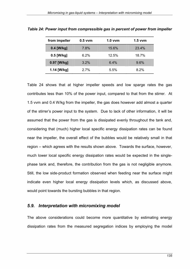
Micromixing in gas-liquid systems – Interpretation with micromixing model
135
Table 24: Power input from compressible gas in percent of power from impeller
from impeller 0.5 vvm 1.0 vvm 1.5 vvm
0.4 [W/kg] 7.8% 15.6% 23.4%
0.5 [W/kg] 6.2% 12.5% 18.7%
0.97 [W/kg] 3.2% 6.4% 9.6%
1.14 [W/kg] 2.7% 5.5% 8.2%
Table 24 shows that at higher impeller speeds and low sparge rates the gas
contributes less than 10% of the power input, compared to that from the stirrer. At
1.5 vvm and 0.4 W/kg from the impeller, the gas does however add almost a quarter
of the stirrer’s power input to the system. Due to lack of other information, it will be
assumed that the power from the gas is dissipated evenly throughout the tank and,
considering that (much) higher local specific energy dissipation rates can be found
near the impeller, the overall effect of the bubbles would be relatively small in that
region – which agrees with the results shown above. Towards the surface, however,
much lower local specific energy dissipation rates would be expected in the single-
phase tank and, therefore, the contribution from the gas is not negligible anymore.
Still, the low side-product formation observed when feeding near the surface might
indicate even higher local energy dissipation levels which, as discussed above,
would point towards the bursting bubbles in that region.
5.9. Interpretation with micromixing model
The above considerations could become more quantitative by estimating energy
dissipation rates from the measured segregation indices by employing the model

Micromixing in gas-liquid systems – Interpretation with micromixing model
136
discussed in chapter 4. The data is presented as and compared relatively (in
percentages) to investigate the bubbles’ and the impeller’s effects.
5.9.1. General comparison
The original model, as suggested in literature (Fournier et al. 1996a; Assirelli et al.
2008b) shows the significant improvement near the surface, by more than an order of
magnitude, as summarised in Table 25. In contrast, the fluctuations near the impeller
are less remarkable, though the actual are still higher than near the surface. The
data in Table 26 is usually at least 2-3 times higher than that in Table 25.
Table 25: Estimates for at pos. 1 (near surface) – using original model
[W/kg] 0.0 vvm [W/kg]
0.5 vvm [W/kg]
1.0 vvm [W/kg]
1.5 vvm [W/kg]
0.40 0.110 0.302 0.610 1.189
0.50 0.136 0.255 0.634 1.141
0.97 0.246 0.403 0.634 1.174
1.14 0.261 0.420 0.666 1.053
Table 26: Estimates for at pos. 2 (near impeller) – using original model
[W/kg] 0.0 vvm [W/kg]
0.5 vvm [W/kg]
1.0 vvm [W/kg]
1.5 vvm [W/kg]
0.40 1.752 1.934 2.458 2.216
0.50 2.144 2.307 2.307 2.612
0.97 3.488 3.105 3.525 3.336
1.14 3.648 3.441 3.992 3.371

Micromixing in gas-liquid systems – Interpretation with micromixing model
137
The model using the adapted interpolation of the most suitable kinetic data, i.e.
estimating an inhibiting effect at the conditions in the stirred tank, shows very similar
trends; though in about an order of magnitude lower absolute values:
Table 27: Estimates for at pos. 1 (near surface) – using adapted model
[W/kg] 0.0 vvm [W/kg]
0.5 vvm [W/kg]
1.0 vvm [W/kg]
1.5 vvm [W/kg]
0.40 0.009 0.033 0.080 0.185
0.50 0.012 0.026 0.083 0.176
0.97 0.025 0.047 0.083 0.182
1.14 0.027 0.050 0.089 0.159
Table 28: Estimates for at pos. 2 (near impeller) – using adapted model
[W/kg] 0.0 vvm [W/kg]
0.5 vvm [W/kg]
1.0 vvm [W/kg]
1.5 vvm [W/kg]
0.40 0.303 0.343 0.465 0.408
0.50 0.391 0.429 0.429 0.502
0.97 0.724 0.625 0.734 0.685
1.14 0.767 0.712 0.859 0.694
Interestingly, the values for position 1 are about an order of magnitude higher than
the calculated power input from the gas. Assuming that the latter is dissipated evenly
throughout the tank, this points at an additional, though still gas-related, factor
contributing towards the significant improvements near the surface. Again, this
suggests bubble bursting as suspected earlier and also discussed in literature
(Boulton-Stone and Blake 1993).

Micromixing in gas-liquid systems – Interpretation with micromixing model
138
5.9.2. Comparisons near surface
Expressing these results in relative terms, i.e. in percent of a reference value, will
allow stronger distinctions between sparging and impeller effects. Moreover, the
modelling section showed that this could be more reliable for quantification than
employing the absolute values.
Therefore, the data for feeding near the surface is given in Table 29 in percent of the
equivalent single-phase condition, i.e. at same impeller power input. This
emphasises the dramatic improvements near the surface and the above conclusions:
Table 29: Estimates for as % of equivalent single-phase value at pos. 1 (near
surface) – to highlight effect of sparging – using adapted model
[W/kg] 0.5 vvm [W/kg]
1.0 vvm [W/kg]
1.5 vvm [W/kg]
0.40 357% 872% 2031%
0.50 221% 697% 1468%
0.97 187% 332% 725%
1.14 182% 327% 584%
These tables refer to data from the adapted model. Other results, including those for
the original approach are very similar and are not shown for brevity.
In order to reflect the influence of the impeller, a comparison to the results at the
lowest power input is given in Table 30. This shows some effect for lower sparge
rates, while the results become relatively independent from the impeller speed
towards 1.5 vvm.

Micromixing in gas-liquid systems – Interpretation with micromixing model
139
Table 30: Estimates for as % of lowest power input for sparged case at pos.
1 (near surface) – to highlight effect of impeller – using adapted model
[W/kg] 0.5 vvm [W/kg]
1.0 vvm [W/kg]
1.5 vvm [W/kg]
0.40 100% 100% 100%
0.50 81% 105% 95%
0.97 144% 105% 98%
1.14 152% 112% 86%
5.9.3. Comparisons near impeller
Such considerations are also of interest for position 2 in order to amplify the
observed fluctuations and to separate between impeller and gas effects more clearly.
Table 31 shows that the deviations at the lower power inputs might indeed be
relevant. Remarkably, the order of magnitude of these changes is roughly in
agreement with the calculated power input from the gas (see Table 24), though here
the experimental error clearly becomes almost equally relevant too. Overall, the
effect of the impeller is dominant, as emphasised in Table 32.
Table 31: Estimates for as % of equivalent single-phase value at pos. 2 (near
impeller) – to highlight effect of sparging – using adapted model
[W/kg] 0.5 vvm [W/kg]
1.0 vvm [W/kg]
1.5 vvm [W/kg]
0.40 113% 154% 135%
0.50 110% 91% 128%
0.97 86% 101% 95%
1.14 93% 112% 90%

Micromixing in gas-liquid systems – Conclusions
140
Table 32: Estimates for as % of lowest power input for sparged case at pos.
2 (near impeller) – to highlight effect of impeller – using adapted model
[W/kg] 0.5 vvm [W/kg]
1.0 vvm [W/kg]
1.5 vvm [W/kg]
0.40 100% 100% 100%
0.50 125% 92% 123%
0.97 182% 158% 168%
1.14 207% 185% 170%
5.10. Conclusions
The effect of gas sparging on micromixing was studied experimentally using the
Iodide/iodate method and a model was applied to that data. The reaction scheme
was found suitable for such measurements, even using air, which confirms earlier
work (Lin and Lee 1997) who, however, used N2.
At constant power input from the impeller, the segregation index near the impeller and
below it was not significantly affected by gas rates up to 1.5 vvm. Applying the incorpora-
tion model to the data confirmed relatively small fluctuations. Near the surface, however,
micromixing was improved significantly with increasing sparge rates and became
relatively independent from impeller power input. This was confirmed in experiments
without power contribution from the impeller, i.e. N = 0 rpm. Overall, the interpretation of
the experimental data using the incorporation model revealed increases in local specific
energy dissipation rate by about an order of magnitude near the surface. Considering all
available information, the significant improvements near the surface, the results without
impeller contribution and simple calculations of the power input from the gas itself,
suggests that the bursting bubbles might be a relevant factor for the effects found.

Micromixing in solid-liquid systems – Introduction
141
6. MICROMIXING IN SOLID-LIQUID SYSTEMS
6.1. Introduction
In addition to chemical reactors with solid catalysts, precipitation and crystallisation
are obvious examples for cases where micromixing might become relevant when
solid particles are present. Even though such systems have been studied before,
conflicting results have been reported especially for stirred tanks, see section 2.3.4.
In this chapter, the effects of a range of different particle sizes and concentrations
were investigated at three feed positions: near the surface, near the impeller and
near . As in the previous chapter, but here for solids, the method is validated,
experimental conditions defined and results from these experiments reported and
interpreted, also using the modelling described in the previous sections. The
experimental results are also discussed in the context of available literature.
6.2. Validation of the experimental method in a liquid-solid system
As for the gas-liquid studies, the Iodide-Iodate method had to be validated for
experiments with added solid particles, In fact, the technique has already been
applied in stirred tanks with glass particles by Villermaux et al. (1994). Unfortunately,
their (unexpected) results had to be corrected later (Guichardon et al. 1995): the
authors explained that there had been losses of iodine during the experimental
procedure. Mass balances showed that adsorption to the glass had not occurred, but
that evaporation during a filtration step had affected the findings.

Micromixing in solid-liquid systems – Power input in the presence of particles
142
In studies employing reaction systems different from the Iodide-Iodate method,
issues with adding solid phases have been reported, e.g. Bennington and co-workers
applied diazo-coupling reactions in suspensions of fibres and had to take disturbing
effects due to adsorption of reactants into account (Bennington and Bourne 1990;
Bennington and Thangavel 1993; Mmbaga and Bennington 1998).
For these reasons, tests similar to those for the gas sparged cases in section 5.2.
were undertaken. Again, iodine/triiodide containing solutions with the added second
phase, here glass beads in various amounts, were stirred and observed over time.
No losses due to the presence of glass beads were found, which agrees with other
authors (Guichardon et al. 1995; Unadkat 2009).
In order to avoid losses during filtration, a fine mesh was installed inside the tank in
front of the sampling pipe. Thanks to this set-up, the glass beads remained in the
vessel and no further treatment of the samples was necessary.
6.3. Power input in the presence of particles
6.3.1. Power measurement results in solid-liquid cases
Figure 46 shows the power number as a function of Reynolds number for single-
phase and with 2.46 wt.% and 11.63 wt.% 500 µm glass beads. As stated in
5.3. Power input in sparged cases, only higher power inputs will be considered valid
here due to technical limitations (rest is plotted in faint colour). Nevertheless, the
trends in Figure 46 agree with what would be expected (see section 2.1.4.): the lower
particle concentration and the single-phase curve are very similar. In contrast, the
power number for the higher concentration is at first lower than the other two curves

Micromixing in solid-liquid systems – Power input in the presence of particles
143
due to the formation of a “false bottom” and then, once sufficient amounts of particles
have become suspended, higher which can be explained with the higher density
around the impeller. A similar result was obtained for 1125 µm particles (data not
shown).
Figure 46: Power number as a function of Reynolds number – with and without
500 µm particles
6.3.2. Conditions for micromixing experiments with particles
From Figure 46 it can be concluded that lower particle concentrations, i.e. up to
2.46 wt.%, do not significantly affect power input and consequently single-phase
impeller speeds can be used for such conditions as well. These are summarised in
Table 33.
Re [-]
2x10⁴ 4x10⁴ 6x10⁴ 8x10⁴ 2x105105
Po
[-]
1
10
single-phase2.46 wt.% 500 m particles11.63 wt.% 500 m particles

Micromixing in solid-liquid systems – Power input in the presence of particles
144
In addition to the 500 µm glass beads, also other sizes, i.e. 150, 250, 625 and
1125 µm particles, were used at such low concentrations. For this range of sizes,
only one power input was employed. In order to suspend the particles as well as
possible, while avoiding surface aeration, an impeller speed of 660 rpm was chosen
for these cases (including single-phase experiments for reference).
Table 33: Impeller speeds for experiments with solid particles
for matching mean specific energy dissipation rates,
[W/kg]
up to 2.46 wt.% [rpm]
11.63 wt.% [rpm]
0.18 300
0.40 395 433
0.50 420 456
0.97 522 548
1.14 552 570
In addition to the experiments with 11.63 wt.% of 500 µm, also a second particle size
was tested for comparison at a higher power input in the range – a discussion on
how the mean specific energy dissipation rate was defined is given on the next page:
for 1.14 W/kg: 1125 µm particles – also at 570 rpm
At this power input, the results of the measurements were very similar for both glass
bead sizes, i.e. 570 and 569.5 rpm for 500 and 1125 µm, respectively.
As demonstrated in part 2.3., particle size is critical for turbulence modulation and,
therefore, the effect of several sizes of glass particles at low particle concentrations,
i.e. up to 2.46 wt.%, was studied at one power input:
for 1.94 W/kg: 150, 250, 500, 625 and 1125 µm particles – at 660 rpm

Micromixing in solid-liquid systems – Power input in the presence of particles
145
It has to be emphasised that it is not obvious how the mean specific energy
dissipation rate should be maintained at the same level as in the single phase case:
it might be based on power per mass of liquid or per total mass, i.e. solid and liquid.
Considering that a model for higher concentrations of suspended particles in earlier
work (Nienow and Conti 1978) assumed power input going into particle abrasion,
elastic deformation and into fluid motion, the second option, power per mass of solid
and liquid, was chosen.
6.3.3. Flow at the chosen conditions
The above conditions are a result of taking several factors into account, e.g. trying to
maintain good particle suspension while avoiding surface aeration. Similar issues
have also been reported by other authors (Barresi 2000; Unadkat 2009). Due to the
range of particle sizes and concentrations investigated here, fully suspending the
particles might be an issue, especially with increasing size and concentration.
Therefore, was calculated according to Zwietering (1958), see equation (2.9), and
the chosen impeller speeds compared to it.
Table 34 gives the impeller speeds for the investigated power inputs as percent of
. The lower power inputs are not expected to be sufficient for fully suspending all
particles and the calculated values show that these stirred speeds indeed are as low
as half . However, Brucato and Brucato (1998) showed that at 80% of almost
all particles are suspended and that the final 20% of are only necessary for
getting the last few particles into suspension. Also, considering that concentration

Micromixing in solid-liquid systems – Power input in the presence of particles
146
gradients have to be expected even above , the values given for particle
concentration will still only be a general indication of the amount of particles
suspended in the vessel and probably not accurately reflect the actual concentration
experienced by the turbulence and chemical reactants near the feed pipe.
Table 34: Suspension state of 500 µm particles over range of power inputs - expressed as percent of
wt.% 300 rpm 420 rpm 522 rpm 552 rpm
0.25% 59.1% 82.8% 102.9% 108.8%
0.75% 51.3% 71.8% 89.2% 94.3%
1.24% 48.0% 67.2% 83.5% 88.3%
2.46% 43.9% 61.5% 76.4% 80.8%
At the highest investigated particle concentration, 11.63 wt.%, fully suspending all
particles was not expected, as equivalent power inputs in the single-phase case
would have led to surface aeration. However, it was not necessary to reach a state
of complete suspension, as the aim was to investigate cloud formation.
Consequently, the criterion was to compare the clouds of 500 and 1125 µm particles
at the same power input. At 570 rpm, 68.2% and 58.0% of was achieved for the
smaller and larger glass beads, respectively.
A photograph of such a cloud of 500 µm particles is shown in Figure 47. The
quiescent liquid which is almost free of particles can be seen at the top, while the
lower parts of the vessel is opaque due to the large amount of glass beads.

Micromixing in solid-liquid systems – Power input in the presence of particles
147
Figure 47: Example of cloud ( = 500 µm; 11.63 vol.%)
In Table 35, the impeller speed, 660 rpm, is expressed as percent of for the
different particle sizes is shown. With these conditions only the biggest glass beads
(1125 µm) at the highest concentration (7.2 vol.%) fall below the 80% of
suggested by Brucato and Brucato (1998). This is in agreement with the visual
observation of the vessel’s bottom which showed most particles being suspended
during the experiments.
Table 35: Suspension state at 660 rpm - expressed as percent of
wt.% 150 µm 250 µm 500 µm 625 µm 1125 µm
0.25% 165.5% 149.4% 130.1% 124.4% 110.6%
0.75% 143.5% 129.6% 112.8% 107.9% 95.9%
1.24% 134.3% 121.3% 105.6% 101.0% 89.8%
2.46% 122.9% 110.9% 96.6% 92.4% 82.1%
7.2% 106.9% 96.5% 84.0% 80.4% 71.5%

Micromixing in solid-liquid systems – Effect of particle size on micromixing in dilute suspensions
148
Nevertheless, the distribution of the glass beads is clearly not uniform even
throughout the cloud, as discussed above and in section 2.1.4. For this reason, the
concentrations of particles for the various experiments must be seen as the amount
present in the tank but they will not represent the actual value in the proximity of the
feed pipe positions.
6.4. Effect of particle size on micromixing in dilute suspensions
As discussed extensively in part 2.3.2, adding a dispersed phase has been shown to
affect turbulence in a range of fluid flows and it has been suggested that particle size
is a critical parameter. In stirred tanks, solid particles might also affect energy
dissipation, but literature is conflicting. These aspects are presented in section 2.3.4.
and in literature (Micheletti and Yianneskis 2004; Unadkat 2009; Hofinger et al.
2011). In spite of the uncertainties, particle size has repeatedly been suggested as
the determining factor whether turbulence augmentation or suppression occurs.
For this reason, this parameter was studied for three feed position: in the impeller
discharge stream, near the surface and in the region of .
6.4.1. Near impeller
Figure 48 shows the results of these experiments for 5 particle sizes over a range of
concentrations at constant impeller speed (and, at these concentrations, constant
power input) for feeding into the impeller discharge stream. Interestingly, no
systematic difference in behaviour according to glass bead size can be seen in this
case, which is unexpected, considering the range of effects presented in literature.
For lower concentrations, the results are actually so close to the liquid-only value that

Micromixing in solid-liquid systems – Effect of particle size on micromixing in dilute suspensions
149
they fall within the error bars. At the highest concentration, all points indicate slightly
worse micromixing, which might be explained by four-way coupling, i.e. some energy
being dissipated by particle-particle interaction. Still, this graph does show the
significance of these deviations.
Figure 48: Effect of particle size in dilute suspensions on the segregation index
as a function of particle concentration – near impeller at 660 rpm
Figure 49 gives the data presented in Figure 48 as percent of the single-phase
equivalent. This might give a clearer view of the magnitude of any deviations
observed and magnifies any effects. Lower amounts of particles, i.e. from about 0.2
to 2 wt.%, the glass beads did not affect micromixing significantly, as any deviations
are usually less than 2% of and always less than 4% which is within the expected
experimental error. This agrees with some literature (Guichardon et al. 1995), but

Micromixing in solid-liquid systems – Effect of particle size on micromixing in dilute suspensions
150
might be in conflict with more recent results (Unadkat 2009) which indicate significant
suppression by more than 20 % of by 100 µm glass beads around 0.5 to 1 vol.%.
In the latter work, the feed was in the region of which may help explain the
differences, in spite of results showing that particles should also affect the region
here studied (Micheletti and Yianneskis 2004).
At concentrations over 2 wt.%, the results drop slightly to about -5 % of , i.e. a
small increase in side-product formation. This drop might be interpreted as still falling
within the experimental error. Taking into account that all particle sizes investigated
follow the same trend, this may, however, be a genuine, though small trend towards
turbulence suppression at these higher particle concentrations.
Figure 49: Effect of particle size in dilute suspensions at several particle
concentrations – in percent of single-phase segregation index – near impeller

Micromixing in solid-liquid systems – Effect of particle size on micromixing in dilute suspensions
151
6.4.2. Near surface
Literature has focused on turbulence modulation in the impeller region, but not near
the surface – even though, in industry, this may be the preferred position for feeding.
Therefore, some experiments were undertaken in this location and the results are
plotted in Figure 50. The segregation indices fluctuate around the single-phase value
and increase slightly at the highest concentration. As suggested above, the higher
particle concentrations might already fall into a region where particle interaction
becomes relevant. The overall effect looks very similar to the result for feeding closer
to the impeller, but the magnitude of the deviation needs to be compared as well.
Figure 50: Effect of particle size in dilute suspensions on the segregation index
as a function of particle concentration – near surface

Micromixing in solid-liquid systems – Effect of particle size on micromixing in dilute suspensions
152
Figure 51 shows the deviations of the segregation indices from the single-phase
reference with all data being within ±2.5% at concentrations up to 2 wt.% of glass
beads. At around 7.2 wt.%, in contrast to the previous results, there only seems to
be an effect with the smallest investigated particles, which is as before, around -5%.
However, the larger particles probably did not get dispersed well enough to reach the
surface at representative concentrations and, therefore, the smaller deviation is
probably less a turbulence modulation effect and more a suspension and dispersion
issue. Unfortunately, this could not be avoided, as reference data was needed and
higher impeller speeds would have caused surface aeration (at least in the single-
phase case and probably also with these low particle amounts). Other setups, like
using different impellers or a differently shaped vessel bottom, might be useful in
future studies. However, the overall effect is small and, in fact, might even still be
considered as within experimental error. Taking the consistent trend of the behaviour
near the impeller and near the surface into account, minor reduction in micromixing
efficiency and energy dissipation rates might be a more reasonable explanation than
arguments regarding measurement errors. A relatively simple explanation would be
that, at higher concentration, the particles interact and dissipate some of the energy,
for instance in not fully elastic collisions. At 7.2 wt.% or 3 vol.%, significant particle
interaction might be expected, since for instance Elghobashi (1994) indicated
turbulence modulation for lower volume fractions. That work would suggest that four-
way coupling becomes a significant factor for the higher particle concentrations.
Consequently, the small deviations found here are attributed to particle interaction,
not turbulence suppression.

Micromixing in solid-liquid systems – Effect of particle size on micromixing in dilute suspensions
153
Figure 51: Effect of particle size in dilute suspensions at several particle
concentrations – in percent of single-phase segregation index – near surface
6.4.3. Near location of highest energy dissipation rates,
As no significant turbulence modulation has been observed near the surface and in
the impeller discharge stream, measurements when feeding into the region of highest
energy dissipation rates are necessary. Unfortunately, as discussed in section 2.3.,
there are already a number of conflicting publications and a range of suggested
mechanisms to explain some aspects of these findings. This section is intended to
contribute to giving a picture of such phenomena especially by also comparing these
results to those from other feed positions in a stirred tank.
Possible effects of particle size and concentration were investigated and Figure 52
gives the results for five sizes as segregation index against amount of particles.
Again, the single-phase value is plotted as a dashed line and, interestingly, behaviour

Micromixing in solid-liquid systems – Effect of particle size on micromixing in dilute suspensions
154
similar to the previous results can be found: at the lowest concentrations the data is
close to the liquid-only case and at the highest concentration some deviation from
that value is seen. This is surprising, considering the reports of turbulence
augmentation and suppression near , which would lead to expectations of more
significant effects – at least more than the size of the error bars.
Figure 52: Effect of particle size in dilute suspensions on the segregation index
as a function of particle concentration – near
Figure 53 gives the deviations as percent of the single-phase value. The graph
shows that all the values are within ±5% which is what might be tolerated as error. In
contrast, Unadkat (2009) found deviations of around 10 to 15% and for one particle
size even around 20% when feeding into of a pitched blade turbine. It is worth
remembering how low is near compared to the other locations – i.e., in this
work, less than 0.05 here instead of almost 0.2 near the surface. This explains the
slightly larger error bars in this feed location compared to others, because small

Micromixing in solid-liquid systems – Effect of particle size on micromixing in dilute suspensions
155
deviations are proportionately more stronger reflected in such small values, i.e. due
to the scale errors become amplified. Nevertheless, the deviations do not follow the
previous trends, as not all values indicate slight turbulence suppression at higher
concentration – assuming that such small changes do actually indicate effects of the
particles on micromixing. Near this feed point, the values seem to diverge, though
not in the way predicted by literature: here the values for small particles point towards
turbulence enhancement and the bigger ones towards suppression. However, it has
to be emphasised again that these deviations are small.
Overall, it is difficult to draw more conclusions from these results than that, if there
are effects, they are relatively small. Interpretation of the data might show more
useful details when energy dissipation rates are discussed instead of segregation
indices. This would also aid connecting these results with those from other methods
like PIV and LDA.
Figure 53: Effect of particle size in dilute suspensions at several particle
concentrations – in percent of single-phase segregation index – near

Micromixing in solid-liquid systems – Effect of solid concentration on micromixing
156
6.5. Effect of solid concentration on micromixing
In the previous section, it was found, for a range of particle sizes, that low
concentrations of glass beads do not affect micromixing in a stirred tank or at least
do so less significantly than would have been expected from reports in literature.
Another aspect is the amount of particles in the system. Therefore, two extremes are
tested: low concentrations, i.e. dilute suspensions, and a higher concentration, i.e. a
dense suspension, in which cloud formation occurs.
6.5.1. Near impeller
Several concentrations of 500 µm particles were tested for a range of power inputs
and the results are summarised in Figure 54. The data points for up to 2.46 wt.%
fluctuate around the single-phase value and do not show any significant patterns.
Therefore, the previous conclusion for small amounts of glass beads is confirmed for
different power inputs – and therefore particle distribution and fluid dynamic
conditions. The higher particle concentration gave a cloud at the impeller speeds
employed during the experiments. In these conditions, micromixing clearly becomes
worse – even at constant power per total mass. If the second option for keeping
mean specific energy dissipation constant, power per liquid mass, had been chosen,
this effect would be even more significant, as the impeller speed would have been
reduced further instead of the increase due to the increase in total mass in this work.
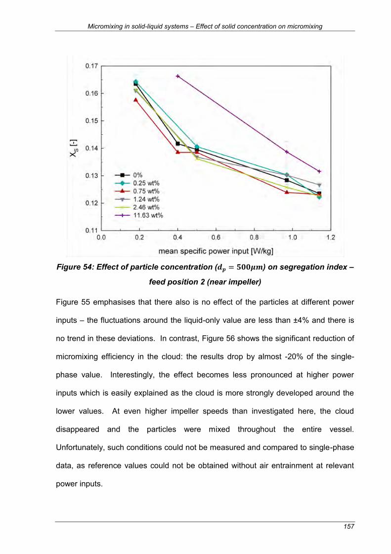
Micromixing in solid-liquid systems – Effect of solid concentration on micromixing
157
Figure 54: Effect of particle concentration ( ) on segregation index –
feed position 2 (near impeller)
Figure 55 emphasises that there also is no effect of the particles at different power
inputs – the fluctuations around the liquid-only value are less than ±4% and there is
no trend in these deviations. In contrast, Figure 56 shows the significant reduction of
micromixing efficiency in the cloud: the results drop by almost -20% of the single-
phase value. Interestingly, the effect becomes less pronounced at higher power
inputs which is easily explained as the cloud is more strongly developed around the
lower values. At even higher impeller speeds than investigated here, the cloud
disappeared and the particles were mixed throughout the entire vessel.
Unfortunately, such conditions could not be measured and compared to single-phase
data, as reference values could not be obtained without air entrainment at relevant
power inputs.

Micromixing in solid-liquid systems – Effect of solid concentration on micromixing
158
Figure 55: Effect of particle concentration ( ) at low particle
concentrations as percent of single-phase segregation index – feed position 2
Figure 56: Effect of particle concentration ( ) at particle conc. with
and without cloud as percent of single-phase segregation index – feed position 2

Micromixing in solid-liquid systems – Effect of solid concentration on micromixing
159
As 500 µm glass beads have resulted in suppression of micromixing and literature
would indicate augmentation due the presence of big(ger) particles, another larger
size was tested. Considering that studying different power inputs has not shown any
significant additional effects or changes in behaviour of the solid-liquid mixtures, one
power input was found sufficient for these purposes. Therefore, Table 36
summarises the data for micromixing when feeding into a cloud at 1.14 W/kg:
Table 36: Effect of cloud on micromixing near impeller
particle size percentage of
500 µm -7.7%
1125 µm -14.2%
Interestingly, the bigger particles lead to an even more significant reduction of
micromixing efficiency. This directly contradicts expected behaviour from turbulence
modulation literature and, therefore, indicates that two-way coupling alone will not aid
interpretation of such cases. As measurable turbulence enhancement is not found in
this case, particle interaction could have become relevant – which is quite reasonable
at such particle concentrations. This is in agreement with the PIV results presented
by Gabriele et al. (2011). However, their argumentation employing turbulence
modulation theories seems less appropriate than considerations of four-way
coupling.
6.5.2. Near surface
Visual observation and literature indicate that fluid circulation and macromixing are
very poor in the clear liquid layer above the cloud. As previous studies did not clearly
state whether feeding occurred in or above the cloud, this section is dedicated to

Micromixing in solid-liquid systems – Effect of solid concentration on micromixing
160
feeding above, while the previous one (section 6.5.1.) was on feeding near the
impeller, i.e. into the cloud.
Figure 57 shows that different power inputs do not change the conclusion for low
particle concentrations: there is no significant effect. For the 11.63 wt.% case,
however, the results for feeding above the cloud do show significantly higher
formation of side-product. This result is not surprising, considering that the fluid in
this region is rather quiescent. Nevertheless, it is relevant, as surface feeds are
popular in industry and data for such a well-defined feed position has not been
shown before.
Figure 57: Effect of particle concentration ( ) on segregation index –
feed position 1 (near surface)

Micromixing in solid-liquid systems – Interpretation with micromixing model
161
As before, a second particle size was tested at 1.14 W/kg and the data is
summarised in Table 37. In this case, the bigger particles lead to better micromixing
than the smaller ones. Hypothetically, this might conform to turbulence modulation
theory, but: there are no particles in the relevant region near the feed pipe. A more
sensible explanation might come from simply looking at the clouds: the bigger
particles lead to a much less well-defined cloud than the smaller ones. Therefore,
the layer above the cloud is less quiescent and micromixing consequently better.
Table 37: Effect of cloud on micromixing near surface
particle size percentage of
500 µm -32.3%
1125 µm -16.9%
6.6. Interpretation with micromixing model
6.6.1. Effect of particle size at low particle concentrations
As lower amounts of particles only had relatively little effect on , the most “extreme”
case will be discussed here: though it might not even fall into a region where only
turbulence modulation is relevant, the changes with 3 vol.% (7.2 wt.%) glass beads
are discussed here. Regarding the feed position, there is most indication from
literature for effects when feeding near . Therefore, the deviations discussed in
6.4.3. are summarised in Table 38 by giving them for different model solutions as the
changes in compared to the single-phase value. Considering that the deviations
of were within experimental error and that such models amplify such differences,
these fluctuations of 20% or less cannot be considered significant. However, other

Micromixing in solid-liquid systems – Interpretation with micromixing model
162
reports in literature showed much larger effects on the segregation index and would,
therefore, indicate much larger changes on local specific energy dissipation rates.
This would support the data presented by Unadkat (2009) which suggested strong
turbulences modulation in PIV and micromixing measurements. As the
concentrations used in that work are different from this work, a more extensive
comparison or even application of the model would not be reasonable.
Table 38: Effect of particle size on – pos. 4 (near ) - 3 vol.% - deviation of
compared to single-phase result
original model diluted + kinetics: Xie et al.
adapted interpolated kinetics
150 µm 17% 20% 20%
250 µm 17% 20% 19%
500 µm 7% 8% 8%
1125 µm -13% -15% -14%
As the changes in the “worst” case are already relatively modest, using the model is
futile for further investigation of other conditions in dilute suspension which show
even less effects in segregation index.
6.6.2. Effect of particle concentration (cloud formation)
While the above gave effects within the range of expected error and less than or
around 20% of estimated specific local energy dissipation rates, clouds did lead to
significant changes in segregation index, which can be expected to translate into
effects on as well. The deviations are again expressed in percent of the
equivalent single-phase values for different models – near the surface and near the
impeller in Table 39 and Table 40, respectively. Table 39 illustrates how much worse

Micromixing in solid-liquid systems – Interpretation with micromixing model
163
micromixing becomes near the surface when clouds are formed: these deviations
suggest drops in by almost or around an order of magnitude, which is especially
remarkable taking into account that the micromixing conditions in this region have
already been found less than ideal in liquid-only measurements. This result fit
surprisingly well with results from LDV measurements in the clear liquid over clouds
by Bittorf and Kresta (2003). They found a drop by 75% for the turbulent RMS
velocity, which is in good agreement with the present results, considering the
differences in the experimental stet-ups and conditions.
Table 39: Effect of clouds on – pos. 1 (near surface)
original model
diluted + kinetics: Xie et
al.
adapted interpolated
kinetics
500 µm -86% -92% -92%
1125 µm -65% -74% -73%
In comparison to the clear liquid layer, the effects in the clouds are not as substantial
but still significant as shown in Table 40. This region is not accessible for laser-
based methods because of the high concentration of solids. This new data gives
insight into such systems, which is especially relevant because such dense
suspensions can be found in industrial processes.
Table 40: Effect of clouds on – pos. 2 (near impeller)
original model
diluted + kinetics: Xie et
al.
adapted interpolated
kinetics
500 µm -27% -34% -33%
1125 µm -39% -48% -47%

Micromixing in solid-liquid systems – Conclusions
164
6.7. Conclusions
The effect of solid particles on micromixing in a stirred tank was investigated using
the iodide/iodate reaction scheme. The method was found suitable for the use with
glass beads and three feed positions were employed for this work: near the surface,
near the impeller and near .
At low concentrations, up to 2.5 wt.%, five sizes of glass beads did not affect the
segregation indices for the feed locations studied, but slightly more side-product was
formed at 7.2 wt.% for feeding near the surface and the impeller. Therefore, it is
concluded that no turbulence modulation, as would have been expected from
corresponding literature, was observed at lower concentrations. In contrast, for both
feed positions, all sizes slightly, but consistently dampen turbulence and micromixing
at the highest concentration which can be attributed to particle-particle interaction.
This might also be expected from the general, well-established literature on particle-
fluid and particle-particle interaction (Elghobashi 1994), though there are
investigations discussing only turbulence modulation for such conditions (see review
in section 2.3.). Near , there, again, was no effect at low concentrations which is
in agreement with some of the literature, e.g. Guichardon et al. (1995), although such
effects have been shown in some previous work on turbulence modulation in stirred
tanks, e.g. Unadkat (2009) and Montante et al. (2010). At 7.2 wt.%, when particle-
particle interaction might already become relevant, the data is more scattered and
the experimental errors become larger than in the other experiments. Nevertheless,
the deviations found here indicate only small effects, even when expressed as
changes in local specific energy dissipation rates calculated from the micromixing

Micromixing in solid-liquid systems – Conclusions
165
model variations, and, overall, correspond well to the trend reported here for the
other two feed positions.
At higher concentrations, when clouds were formed, micromixing was consistently
worse than in the equivalent single-phase case – interestingly, in the clear liquid layer
and also in the cloud. This, again, does not point towards the expected effects due
to turbulence modulation but more towards four-way coupling. The high segregation
indices when feeding into the clear liquid above the cloud emphasise the importance
of feed pipe positioning.

Micromixing in liquid-gas-solid systems – Introduction
166
7. MICROMIXING IN LIQUID-GAS-SOLID SYSTEMS
7.1. Introduction
Three-phase systems consisting of sparged gas bubbles and solid particles in liquids
can be found in industrial processes like oxidation, hydrogenation and
polymerisation. In spite of the relevance to real applications, such conditions are still
poorly understood and especially micromixing data has not been reported.
Considering the effects found in the previous chapters on gas-liquid and solid-liquid
cases, micromixing will be investigated near the surface and near the impeller, for
dilute and dense suspensions over a range of sparge rates while keeping power
input from the impeller constant. As the validation of the method has already been
covered before (chapters 5.2. and 6.2.), power measurement data will be presented
first and then micromixing results will be shown and discussed. Again, the
micromixing model from chapter 4 will be applied for further interpretation of the data.
7.2. Power input in 3-phase (l-g-s) system
7.2.1. Power measurement results in liquid-gas-solid cases
As in the previous parts, power data was necessary because the experiments are set
out to run at equivalent power inputs. At low particle concentrations of 1.24 wt.%, the
measured power was very similar, i.e. deviations were within experimental error, to
the corresponding gas-only results for the three sparge rates investigated. This is in
agreement with literature, e.g. Warmoeskerken et al. (1984) who found that up to
5 wt.% did not affect sparged power inputs.

Micromixing in liquid-gas-solid systems – Power input in 3-phase (l-g-s) system
167
When sparging the cloud, i.e. at the higher particle concentration, power had to be
measured. This was done for both sizes of glass beads employed. The results are
plotted in Figure 58 for the 500 µm particles and in Figure 59 for the 1125 µm ones.
The general trends of both graphs agree with literature (Chapman et al. 1983a;
Frijlink et al. 1990; Roman and Tudose 1997).
Figure 58: Relative power input as a function of gas flow number – gassed with
particles – 500 µm and 11.63 wt.%
micromixing experimentsmicromixing experiments
micromixing experiments
micromixing experiments

Micromixing in liquid-gas-solid systems – Power input in 3-phase (l-g-s) system
168
Figure 59: Relative power input as a function of gas flow number – gassed with
particles – 1125 µm and 11.63 wt.%
Maxima of Pg/P where gross recirculation starts to lead to drops in gassed power can
be seen on both graphs and also some of the minima at NCD are captured even
though the measurements are not expected to be accurate at such low power inputs.
7.2.2. Conditions for micromixing experiments with gas and particles
As low amounts of particles did not affect the gassed power input, the impeller
speeds for the gas-liquid conditions, see Table 21, were used for the three-phase
experiments with 1.24 wt.% Ballotini. In the case of 11.63 wt.%, the impeller speeds
were adapted for both particle sizes as summarised in Table 41 to match the power
input to 1.14 W/kg.
micromixing experiments

Micromixing in liquid-gas-solid systems – Power input in 3-phase (l-g-s) system
169
As in the solid-liquid considerations, the question of keeping power constant per total
mass or per liquid mass was not straightforward. The same considerations as in
section 6.3.2. led to the choice of constant power per total mass.
Table 41: Impeller speeds for three-phase experiments with 11.63 wt.% for matching mean specific energy dissipation rate,
for 500 µm
[rpm] for 1125 µm
[rpm]
0.5 vvm 665 670
1.0 vvm 712 715
1.5 vvm 775 758
7.2.3. Flow at the chosen conditions
For the lower particle concentration, the flow appeared similar to the gas-liquid
equivalents. Due to the presence of the gas bubbles, the degree of suspension and
distribution of the particles in the tank could not be observed as accurately as at
solid-liquid conditions. Nevertheless, suspension of 1.24 wt.% glass beads at the
chosen sparge rates appeared complete when observing the tank through the
bottom.
The conditions for the micromixing experiments with the sparged cloud are indicated
in Figure 58 and Figure 59. It can be seen that they are all near the maximum of
Pg/P between complete gas dispersion and gross gas recirculation. Visual
observation confirmed that the impeller was clearly not flooded and that significant
interaction of gas, liquid and impeller was taking place. Regarding solid suspension,
the aim for the higher concentration was not necessarily to reach or - instead

Micromixing in liquid-gas-solid systems – Dilute, sparged suspension
170
any effects of gas bubbles on the poor micromixing in the presence of a cloud was of
interest. To get an impression of how well the particles may be expected to get
suspended, equation (2.9) was employed, although this is will only give general
estimates as the correlation was obtained for larger Rushton turbines. The results
are summarised in Table 42 – expressed as percentage of calculated for the
respective actually used impeller speeds (see previous section):
Table 42: Suspension state for dilute and dense suspensions over range of sparge rates - expressed as percent of
1.24 wt.% 11.63 wt.%
250 µm 500 µm 1125 µm 500 µm 1125 µm
0.5 vvm 117.06% 102.56% 87.78% 76.94% 66.24%
1.0 vvm 120.06% 105.80% 91.09% 79.78% 68.77%
1.5 vvm 124.22% 110.05% 95.28% 84.18% 70.98%
Unfortunately, visual observation is only possible to a limited extent at such high
fractions of added phases (therefore, no image is given). With the lower amounts of
glass beads, visual observation through the bottom of the tank confirmed that all
particles were fully suspended as suggested in Table 42.
7.3. Dilute, sparged suspension
In chapter 5, it was shown that gas bubbles do not significantly affect micromixing in
the impeller discharge stream when the power input from the impeller is kept
constant. Small amounts of solid particles did not lead to considerable effects either,
as presented in chapter 6. Here, the combination of gas and small amounts of solid
particles is investigated.

Micromixing in liquid-gas-solid systems – Dilute, sparged suspension
171
7.3.1. Near impeller
Figure 60 shows the segregation indices in sparged dilute suspensions for 3 particle
sizes as a function of gas flow rate. For reference, the equivalent data from single-
phase and gas-liquid experiments is plotted in this graph as well. Overall, these
three-phase results are close to the liquid and g-l data – especially considering the
size of the error bars, the deviations appear relatively small. However, there seems
to be a slight drop in segregation index of the g-s-l cases with increasing amounts of
gas. Though this trend is only small and within the error bars, it is consistent for all
three particle sizes.
Figure 60: Segregation index as a function of gassing rate in dilute suspension
(1.24 wt.%) - feed near impeller
As in previous chapters, the results are also given as the deviation from reference
data. There are three options: compared to single-phase, gas-liquid or solid-liquid
which will be discussed in the following paragraphs. Figure 61 emphasises that there

Micromixing in liquid-gas-solid systems – Dilute, sparged suspension
172
might be a small effect of the bubbles and particles at 0.5 vvm, but that the results
stay close to the single-phase results. Three-phase micromixing in the impeller
discharge stream seems to be, within experimental error, relatively unaffected by the
added phases. In order to minimise errors due to the power measurements which
might skew the comparison with single-phase data, the results are compared to the
g-l equivalents in Figure 62. This might highlight effects of the combination of
particles and bubbles on micromixing. Figure 62, however, does not show any
significant trends and the deviations of usually less than 5% could be considered
within the expected error. Still, the consistency of the deviations is surprisingly good
and, if effects are found in other feed positions, these results might be seen in a
different light.
Figure 61 : Effect of particle size and sparge rate on micromixing – in percent
of single-phase segregation index – near impeller

Micromixing in liquid-gas-solid systems – Dilute, sparged suspension
173
Figure 62 : Effect of particle size and sparge rate on micromixing – in percent
of gas-liquid segregation index – near impeller
7.3.2. Near surface
As with the above data for feeding near the impeller, Figure 63 shows liquid-only,
gas-liquid and three-phase segregation indices as a function of sparge rate. The
reference data follows a consistent trend with increasing gas flow: micromixing is
significantly improved. The same tendency is found for the dilute, sparged
suspension. The absolute values, however, are higher than in the gas-liquid case,
i.e. micromixing becomes worse near the surface when solid particles are added to a
gas-liquid stirred tank.

Micromixing in liquid-gas-solid systems – Dilute, sparged suspension
174
Figure 63: Segregation index as a function of gassing rate in dilute suspension
(1.24 wt.%) - feed near surface
To quantify these deviations, they are expressed as percent of the reference
segregation index again. The comparison to the liquid-only equivalent in Figure 64,
as expected from the absolute values, shows significant improvement of up to about
15% at 1.5 vvm, though this is lower than the improvement of up to 30% in the g-l
case without any solid particles. Interestingly, there seems to be very little, if any,
difference between the 3 tested particle sizes. In order to magnify the effect of the
particles, a comparison to the gas-liquid data is drawn in Figure 65. This graph
clearly illustrates that particles consistently reduce the improvements in micromixing
that had been observed under gassed conditions near the surface. It might be worth
noting that there is a slight downward trend in this plot, i.e. the effect of the particles
might become more significant – though, taking the error bars into account, this might

Micromixing in liquid-gas-solid systems – Dilute, sparged suspension
175
only be a small effect. It could be explained by a different solids distribution in the
tank with increasing gas rate at constant power input. The trend in Table 42 for
instance indicates improvements in suspending the particles which might contribute
to the observed trend, as one might expect more glass beads to become relevant to
the flow once they are suspended. The slight increase for the largest solids at
1.5 vvm might be also attributed to experimental error or to these particles settling
more easily and therefore not reaching relevant regions in as significant numbers as
the smaller ones. Unfortunately, no relevant information could be found in literature
on particle distribution in three-phase stirred tanks and further work is needed.
Another option could be a possible interaction of bubbles and particles, for instance
stronger or reduced coalescence of the bubbles (Nienow et al. 1986).
Figure 64 : Effect of particle size and sparge rate on micromixing – in percent
of single-phase segregation index – near surface

Micromixing in liquid-gas-solid systems – Dilute, sparged suspension
176
Figure 65 : Effect of particle size and sparge rate on micromixing – in percent
of gas-liquid segregation index – near surface
Such micromixing measurements in 3-phase stirred tanks have not been reported in
open literature before. In addition there is no information from turbulence
measurements, but the consistent trend in the presented data might be discussed in
the context of results found in related phenomena. For instance, a number of mass
transfer studies would be available but, considering the complexity of the topic with
sensitivity to particle properties, surfactants (Vazquez et al. 2000) and ionic strength
(Zuidervaart et al. 2000), also such data cannot be employed. Therefore, further
work on three-phase systems e.g. detailed information on particle distribution and
velocity fields, for instance from PEPT, would be interesting.

Micromixing in liquid-gas-solid systems – Sparged cloud
177
7.4. Sparged cloud
In addition to sparged, dilute suspensions, also cases with higher solids
concentrations were investigated. The results are summarised here.
7.4.1. Near impeller
Figure 66 shows that the results for the 1125 µm cloud are close to the single-phase
reference data, but the sparged 500 µm cloud consistently gives more side-product,
i.e. worse micromixing. Interestingly, both three-phase graphs show a segregation
index peak at 1 vvm and then drop at 1.5 vvm. The significance of these deviations,
however, cannot be discussed from this graph and comparisons as percent of single-
phase, gas-liquid and solid-liquid are given in Figure 67, Figure 68 and Figure 69,
respectively. Figure 67 confirms that, near the impeller, micromixing in the sparged
cloud of 1125 µm particles is similar to the liquid-only behaviour, as the deviations
are less than 4% of segregation index and therefore within the error expected for
such experiments. In contrast, a dampening effect of the cloud of smaller particles
can be seen, especially at 1 vvm with -13.5% deviation in segregation index.

Micromixing in liquid-gas-solid systems – Sparged cloud
178
Figure 66: Segregation index as a function of gassing rate in dense suspension
(11.63 wt.%) - feed near impeller
Figure 67 : Effect of particle size and sparge rate on micromixing – in percent
of single-phase segregation index – near impeller

Micromixing in liquid-gas-solid systems – Sparged cloud
179
Considering that the gas sparging had no significant effect on micromixing near the
impeller, it is not surprising that the trend in Figure 68 is comparable to the single-
phase comparison in Figure 67. Again, the sparged cloud of larger particles leads to
little deviations in micromixing efficiency, while the smaller ones do cause significant
suppression. This does not reflect the dominant effect of the impeller observed in
gas-liquid cases anymore, but at least for the larger particles the cloud seems to
have been compensated for.
Figure 68 : Effect of particle size and sparge rate on micromixing – in percent
of gas-liquid segregation index – near impeller
Figure 69 allows the comparison to the cloud and shows that a consistent
improvement for the 1125 µm Ballotini occurs when sparging, but very little effect for
the cloud of smaller particles. Interestingly, there is still a dip to -5% of segregation
index at 1 vvm compared to the solid-liquid case which might be within experimental
error, considering that the power input had to be measured too. Comparisons for a

Micromixing in liquid-gas-solid systems – Sparged cloud
180
second feed position might give a better indication of whether the deviations at 1 vvm
need more attention or if they can be neglected.
Figure 69 : Effect of particle size and sparge rate on micromixing – in percent
of solid-liquid segregation index – near impeller
Overall, it is remarkable that the dampening effect of the cloud of larger particles,
which resulted in a drop of 14.2% in the unsparged experiments compared to liquid-
only, seems to be fully compensated for by the presence of the gas bubbles. On the
other hand, the smaller particles also only gave a reduction of 7.7% compared to
single-phase at this power input, but that cloud seems to be less affected by the
sparging.
7.4.2. Near surface
On their own, the above results do not give a full picture of the three-phase system
and similar experiments were performed for feeding near the liquid surface. A clear

Micromixing in liquid-gas-solid systems – Sparged cloud
181
layer of liquid with poor micromixing (see section 6.5.2.) would normally be found in
this location above the cloud, but the gas bubbles might affect this.
Figure 70 shows the downward trend of the single-phase and gas-liquid data for
reference and some fluctuating but for both particle sizes consistent behaviour. At
0.5 vvm, feeding above both sparged clouds leads to more side-product than in the
equivalent sparged case. In fact, the data is close to the single-phase result at the
same impeller power input. Interestingly, the segregation indices drop below the
reference data at 1 vvm and then increase again slightly at 1.5 vvm. This is different
from the previous consistently higher result in the more dilute suspension (see
section 7.4.2.), but again shows deviations at 1 vvm, as already noted for feeding
near the impeller at the same conditions. Moreover, the errors reach up to 5.5%
which is relatively encouraging, considering up to 25% error reported by Barresi
(1997) for high particle concentrations in 2-phase experiments.
Figure 70: Segregation index as a function of gassing rate in dense suspension
(11.63 wt.%) – feed near impeller

Micromixing in liquid-gas-solid systems – Sparged cloud
182
In order find an indication for the trends in Figure 70, the data is compared to the
three reference options. Firstly, the percentages of single-phase data are plotted in
Figure 71, which confirms that the results at 0.5 vvm are the same as in the liquid
only experiments, while 1.0 and 1.5 vvm lead to significant improvements in spite of
the 11.63 wt.% particles in the tank. The previously observed direct dependence on
gas sparge rate is not found in this case, though it clearly improves micromixing in
the higher range investigated.
Figure 71 : Effect of particle size and sparge rate on micromixing – in percent
of single-phase segregation index – near surface
Figure 72 confirms the point that the improvements are not directly related to the gas
rate and the deviations at 1 vvm are especially clear in this graph. While it can be
argued that in these conditions, the 500 µm solids cloud only has a negligible effect
on micromixing, there is significant improvement with the larger particles, i.e. 13.6 %
deviation from the g-l result. Figure 73 emphasises that sparging the clouds

Micromixing in liquid-gas-solid systems – Sparged cloud
183
improves micromixing near the surface for all conditions – compared to the cloud
equivalents, which had to be expected due to the poor results found in those
reference cases. It might, however, be argued that micromixing still improved from
0.5 to 1.0 vvm and then stabilised around that value. This would put the data at
1.0 vvm more into context with the rest of the results, instead of being an
unexplained fluctuation. On the other hand, these trends are consistent and the
results near the impeller already showed slight deviations at 1.0 vvm as well.
Unfortunately, the mixture was opaque at these conditions, so even visual
observations of the flow were only possible to a limited extent and did not aid
understanding of the results. New measurement methods, however, might give
detailed insights into liquid and solid behaviour of such complex flows (Guida 2010)
and might help interpretation.
Figure 72 : Effect of particle size and sparge rate on micromixing – in percent
of gas-liquid segregation index – near surface

Micromixing in liquid-gas-solid systems – Sparged cloud
184
Figure 73 : Effect of particle size and sparge rate on micromixing – in percent
of solid-liquid segregation index – near surface
As mentioned above, such studies in gas-solid-liquid stirred tanks have not been
performed before, but other relevant factors like flow field and particle distribution in
the vessel are also not as well studied as in dilute systems. However, it has been
found that the significant increases in macromixing time due to cloud formation can
be reduced back to near single-phase levels by gas sparging (Nienow and Bujalski
2002). This follows a similar line as the micromixing data presented here, but further
investigation in particular of the flow field might be useful for feed pipe positioning.
In addition to these relatively qualitative comparisons, a more quantitative look, in
particular at energy dissipation, could be useful for industry.
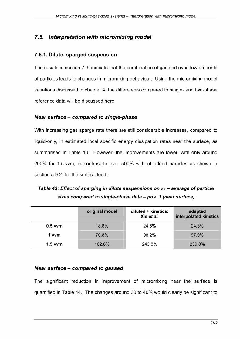
Micromixing in liquid-gas-solid systems – Interpretation with micromixing model
185
7.5. Interpretation with micromixing model
7.5.1. Dilute, sparged suspension
The results in section 7.3. indicate that the combination of gas and even low amounts
of particles leads to changes in micromixing behaviour. Using the micromixing model
variations discussed in chapter 4, the differences compared to single- and two-phase
reference data will be discussed here.
Near surface – compared to single-phase
With increasing gas sparge rate there are still considerable increases, compared to
liquid-only, in estimated local specific energy dissipation rates near the surface, as
summarised in Table 43. However, the improvements are lower, with only around
200% for 1.5 vvm, in contrast to over 500% without added particles as shown in
section 5.9.2. for the surface feed.
Table 43: Effect of sparging in dilute suspensions on – average of particle
sizes compared to single-phase data – pos. 1 (near surface)
original model diluted + kinetics: Xie et al.
adapted interpolated kinetics
0.5 vvm 18.8% 24.5% 24.3%
1 vvm 70.8% 98.2% 97.0%
1.5 vvm 162.8% 243.8% 239.8%
Near surface – compared to gassed
The significant reduction in improvement of micromixing near the surface is
quantified in Table 44. The changes around 30 to 40% would clearly be significant to

Micromixing in liquid-gas-solid systems – Interpretation with micromixing model
186
industrial processes. Nevertheless, the improvements shown in Table 43 still
indicate major advantages of such three-phase systems over single-phase cases at
equivalent mean specific power inputs. Of course, also other factors like flow stability
also have to be considered for real multi-phase applications.
Table 44: Effect of sparging in dilute suspensions on – average of particle
sizes compared to gas-liquid data – pos. 1 (near surface)
original model diluted + kinetics: Xie et al.
adapted interpolated kinetics
0.5 vvm -26.1% -32.0% -31.8%
1 vvm -33.1% -40.1% -39.8%
1.5 vvm -34.8% -42.2% -41.8%
Near impeller – compared to single-phase
The deviations of the segregation indices were much smaller near the impeller, in
fact roughly within experimental error, and further quantification of these changes
might indicate whether further studies are needed or whether the deviations can be
considered negligible.
The largest changes in Table 45 are around 20% and, like those found for the most
“extreme” dilute s-l case, indicate only a small, though consistent effect. For these
condition there is, however, more reference data, i.e. also the s-l results, which
should give similar values as found here, considering the small effect found for
particles near the impeller.

Micromixing in liquid-gas-solid systems – Interpretation with micromixing model
187
Table 45: Effect of sparging in dilute suspensions on – average of particle
sizes compared to single-phase data – pos. 2 (near impeller)
original model diluted + kinetics: Xie et al.
adapted interpolated kinetics
0.5 vvm -18.4% -22.9% -22.6%
1 vvm -13.1% -16.5% -16.2%
1.5 vvm -4.7% -5.9% -5.8%
Near impeller – compared to gassed
As expected, the values in Table 46 are similar to the equivalents in Table 45 and
confirm that there is an effect, which might be considered small compared to the
large changes near the surface.
Table 46: Effect of sparging in dilute suspensions on – average of particle
sizes compared to gas-liquid data – pos. 2 (near impeller)
original model diluted + kinetics: Xie et al.
adapted interpolated kinetics
0.5 vvm -13.5% -16.9% -16.7%
1 vvm -20.6% -25.6% -25.3%
1.5 vvm 3.2% 4.2% 4.1%
7.5.2. Sparged cloud
Near surface
As the patterns found for the sparged cloud did not show a clear pattern, the data will
be expressed as deviation from the single-phase results using the model variations.
Firstly, the effect near the surface is summarised in Table 47 and Table 48 for 500

Micromixing in liquid-gas-solid systems – Interpretation with micromixing model
188
and 1250 particles, respectively. At 0.5 vvm, the deviations are relatively small,
around -7 to 11% of the single-phase value. The effect of the gas bubbles, however,
becomes more noticeable, with improvements by several 100%, at higher gas sparge
rates. This agrees with the results from the other gassed cases, but the correlation is
not as clear anymore for the sparged cloud. Actually, the consistent improvements at
1 vvm stand out and comparisons for both particle sizes to the gas-liquid equivalents,
in Table 49 and Table 50, emphasise this point: while the solid’s negative effect is
reflected in the estimated energy dissipation rates at 0.5 vvm, there are
improvements for both particle sizes at 1 vvm and again worse results at 1.5 vvm.
The improvements near the surface, even compared to gas-liquid, might indicate that
the particles affect the gas bubbles for instance enhancing coalescence, which might
lead to more dramatic bursts at the top, or leading to some other turbulence
enhancing effect. Unfortunately, the changes of behaviour cannot be explained at
this point, because there is not enough information on such three-phase fluid flows.
With consideration of these changes near the surface, the feed position near the
impeller needs to be addressed as well.
Table 47: Effect of sparging in dense suspensions on – 500 particles –
compared to liquid-only data – pos. 1 (near surface)
original model diluted + kinetics: Xie et al.
adapted interpolated kinetics
0.5 vvm -6% -7% -7%
1 vvm 205% 316% 310%
1.5 vvm 153% 227% 223%

Micromixing in liquid-gas-solid systems – Interpretation with micromixing model
189
Table 48: Effect of sparging in dense suspensions on – 1250 particles –
compared to liquid-only data – pos. 1 (near surface)
original model diluted + kinetics: Xie et al.
adapted interpolated kinetics
0.5 vvm 8% 11% 11%
1 vvm 445% 775% 755%
1.5 vvm 367% 619% 604%
Table 49: Effect of sparging in dense suspensions on – 500 particles –
compared to gas-liquid data – pos. 1 (near surface)
original model diluted + kinetics: Xie et al.
adapted interpolated kinetics
0.5 vvm -41% -49% -49%
1 vvm 19% 25% 25%
1.5 vvm -37% -45% -45%
Table 50: Effect of sparging in dense suspensions on – 1250 particles –
compared to gas-liquid data – pos. 1 (near surface)
original model diluted + kinetics: Xie et al.
adapted interpolated kinetics
0.5 vvm -33% -40% -39%
1 vvm 113% 164% 161%
1.5 vvm 16% 21% 20%
Near impeller
Table 51 and Table 52 give the specific energy dissipation rates near the impeller for
500 and 1125 particles, respectively, compared to the single-phase case. In
Table 53 and Table 54 this data is given relative to the gas-liquid data. As gas-

Micromixing in liquid-gas-solid systems – Interpretation with micromixing model
190
sparging did not affect micromixing near the impeller, the results in these table
groups are very similar: while the 500 particles do still dampen turbulence in the
cloud, the one with the larger solids seems to have been broken up by the gas
sparging. Even though the 1125 glass beads had a stronger effect at this feed
position without gas, the cloud was less pronounced. This might explain why with is
more easily affected by changes in the flow. Interestingly, the deviation at 1 vvm can
also be seen with the smaller particles in this case, but neither visual observation of
the flow nor the limited knowledge of such flows aids understanding of these novel
results. They do, however, give valuable information on micromixing and also feed
pipe positioning in multi-phase stirred reactors.
Table 51: Effect of sparging in dense suspensions on – 500 particles – compared to liquid-only data – pos. 2 (near impeller)
original model diluted + kinetics: Xie et al.
adapted interpolated kinetics
0.5 vvm -25% -31% -30%
1 vvm -43% -51% -50%
1.5 vvm -18% -22% -22%
Table 52: Effect of sparging in dense suspensions on – 1250 particles – compared to liquid-only data – pos. 2 (near impeller)
original model diluted + kinetics: Xie et al.
adapted interpolated kinetics
0.5 vvm -5% -6% -6%
1 vvm -5% -7% -7%
1.5 vvm 18% 23% 23%

Micromixing in liquid-gas-solid systems – Conclusions
191
Table 53: Effect of sparging in dense suspensions on – 500 particles –
compared to gas-liquid data – pos. 2 (near impeller)
original model diluted + kinetics: Xie et al.
adapted interpolated kinetics
0.5 vvm -20% -25% -25%
1 vvm -48% -56% -56%
1.5 vvm -11% -14% -14%
Table 54: Effect of sparging in dense suspensions on – 1250 particles –
compared to gas-liquid data – pos. 2 (near impeller)
original model diluted + kinetics: Xie et al.
adapted interpolated kinetics
0.5 vvm 1% 1% 1%
1 vvm -14% -17% -17%
1.5 vvm 27% 36% 36%
7.6. Conclusions
Micromixing in a gas-solid-liquid stirred tank was investigated using the Iodide/iodate
reaction scheme, using dilute and dense suspensions for two particle sizes over a
range of gas sparge rates while keeping mean specific energy input constant.
Experimental conditions were chosen to give good particle suspension while still
allowing reference measurements without entrainment of air from the surface.
While low concentrations of glass beads had not affected micromixing in the solid-
liquid measurements, it was found that already these small amounts lower
micromixing efficiency compared to just sparged conditions. In sparged clouds, the
effects were consistent but less straight-forward to summarise: the gas bubbles

Micromixing in liquid-gas-solid systems – Conclusions
192
improved micromixing near the surface, compared to the very poor solid-liquid results
and, overall, also to the single-phase ones. Near the impeller, there clearly were
effects due to sparging the cloud. However, these cannot be explained at this point
but seem to depend on aeration rate and particle size.

Conclusions and future work – Conclusions – discussed by chapter
193
8. CONCLUSIONS AND FUTURE WORK
8.1. Conclusions – discussed by chapter
The aims set out in the introduction in section 1.1 have been addressed throughout
this thesis and the conclusions are given here briefly. For clarity, they are
summarised for each chapter separately.
Incorporation model: adaption and its use to interpret experimental data
In order to quantify experimental results obtained from the iodide/iodate method,
employing a reliable micromixing model would be useful, but, so far, such
approaches have not been very successful for this reaction scheme. This might be
explained by kinetic data on the Dushman reaction used in previous studies. In
addition, the sulphuric acid has been assumed to be fully dissociated which has been
shown to be wrong. Therefore, the incorporation model was extended to include the
ionisation of the sulphuric acid and a range of kinetic rate laws from literature were
tested. It was found that such modelling is useful for comparison purposes.
Moreover, the adapted version of the model employing estimated kinetic behaviour
for these specific conditions gives realistic absolute values for local specific energy
dissipation rates. At the moment, it has to be concluded that there is still need for
information on the chemistry involved. However, some steps in this direction have
been made here and, once new data becomes available, the variations of the
Incorporation model as presented here can be adapted accordingly.

Conclusions and future work – Conclusions – discussed by chapter
194
Micromixing in gas-liquid systems
The suitability of using air for experiments with the Iodide/Iodate reaction scheme
was confirmed and three feed positions were studied. There was no effect of gas
sparging for feeding near the impeller, when power from the impeller was kept
constant, and also little, if any, effect below the impeller. Near the free surface,
however, there were significant improvements with increasing gas sparge rate.
Estimates from the micromixing model suggest increases of up to 2000% compared
to the single-phase equivalents which indicates positive effects for such industrial
applications, though even higher micromixing efficiencies were still found for feeding
near the impeller.
Micromixing in solid-liquid systems
The use of glass beads was validated for use with the employed reaction scheme.
Considering the conflicting literature, the possible effects of a range of particle sizes
and concentrations were investigated for feeding near the surface, near the impeller
and at . At low concentrations, when particle interaction was not significant,
micromixing was not affected by the presence of the solids. When particle interaction
became relevant, i.e. in more dense suspensions, micromixing became worse.
Especially the formation of clouds leads to significant damping, in the cloud and even
more in the clear liquid layer above the cloud. This clearly showed the importance of
feed pipe positioning. The effects were also evaluated using the micromixing model.
In literature, a small amount of information on turbulence levels above a solids cloud
has been reported and good agreement with the results presented here has been
found.

Conclusions and future work – Suggestions for future work
195
Micromixing in liquid-gas-solid systems
Even low amounts of solid particles have been found to negatively affect micromixing
under gas-solid-liquid conditions compared to just gas-liquid, although this is not the
case in solid-liquid equivalents. At higher solids concentration, i.e. when cloud
formation occurs, gas sparging improved micromixing near the surface compared to
feeding into the clear liquid layer without gas bubbles. Overall, complex behaviour
was found at these conditions for feeding near the surface and near the impeller.
Unfortunately, there is little information on fluid flow behaviour for these conditions
and, therefore, explanation of the observed micromixing data is difficult.
8.2. Suggestions for future work
Although a range of questions and tasks have been tackled, further work can, of
course, be done in this context. Some new results might be studied from different
points of view to find explanations for the observations made here and a few other
ideas or suggestions could be followed in the future.
For the reaction scheme itself, further studies on the kinetics are necessary,
especially work considering the conditions of micromixing experiments in stirred
tanks. This should allow adequate comparison of different reactant concentrations
and ultimately give a quantitatively reliable method.
Such data could be easily applied to the presented model variations.
Although light has been shed on the effect of the presence of solid particles, it is still
a conflicting topic in mixing literature and a smaller study comparing different flows,

Conclusions and future work – Suggestions for future work
196
i.e. from a Rushton turbine and pitched-blade impeller, using competing reactions
and PIV would be of interest. In addition, a dished bottom might allow better solid
suspension without air entrainment from the surface which would widen the range of
possible experimental conditions.
There is still a lack of knowledge on details of fluid flow and particle distribution in
three-phase systems. This is limiting for the interpretation of the results found here.
However, newer methods like PEPT could soon give new insights into such systems.

References
197
REFERENCES
Agreda B., J. A., R. J. Field and N. J. Lyons (2000). "Kinetic Evidence for Accumulation of Stoichiometrically Significant Amounts of H2I2O3 during the Reaction of I- with IO3." The Journal of Physical Chemistry A 104(22): 5269-5274.
Anderson, J. D. (1995). Computational fluid dynamics: the basics with applications. New York ; London, McGraw-Hill.
Argoul, F., A. Arneodo, G. Grasseau, Y. Gagne, E. J. Hopfinger and U. Frisch (1989). "Wavelet analysis of turbulence reveals the multifractal nature of the Richardson cascade." Nature 338(6210): 51-53.
Armenante, P. M., C. Luo, C.-C. Chou, I. Fort and J. Medek (1997). "Velocity profiles in a closed, unbaffled vessel: comparison between experimental LDV data and numerical CFD predictions." Chemical Engineering Science 52(20): 3483-3492.
Ascanio, G., B. Castro and E. Galindo (2004). "Measurement of Power Consumption in Stirred Vessels--A Review." Chemical Engineering Research and Design 82(9): 1282-1290.
Assirelli, M. (2004). Micromixing studies in turbulent stirred baffled and unbaffled vessels agitated by a Rushton turbine: an experimental study. School of Engineering, Chemical Engineering, University of Birmingham. PhD thesis.
Assirelli, M., W. Bujalski, A. Eaglesham and A. W. Nienow (2002). "Study Of Micromixing in a Stirred Tank Using a Rushton Turbine: Comparison of Feed Positions and Other Mixing Devices." Chemical Engineering Research and Design 80(8): 855-863.
Assirelli, M., W. Bujalski, A. Eaglesham and A. W. Nienow (2005). "Intensifying micromixing in a semi-batch reactor using a Rushton turbine." Chemical Engineering Science 60(8-9): 2333-2339.
Assirelli, M., W. Bujalski, A. Eaglesham and A. W. Nienow (2008a). "Macro- and micromixing studies in an unbaffled vessel agitated by a Rushton turbine." Chemical Engineering Science 63(1): 35-46.
Assirelli, M., S. P. Lee and A. W. Nienow (2011a). "Further Studies of Micromixing: Scale-Up, Baffling and Feed Pipe Backmixing." Journal of Chemical Engineering of Japan 44(11): 901-907.
Assirelli, M., S. P. Lee and A. W. Nienow (2011b). "Further Studies of Micromixing: Scale-Up, Baffling and Feed Pipe Backmixing." Journal of Chemical Engineering of Japan 44.
Assirelli, M., E. J. W. Wynn, W. Bujalski, A. Eaglesham and A. W. Nienow (2008b). "An extension to the incorporation model of micromixing and its use in estimating local specific energy dissipation rates." Industrial & Engineering Chemistry Research 47(10): 3460-3469.
Aubin, J., M. Ferrando and V. Jiricny (2010). "Current methods for characterising mixing and flow in microchannels." Chemical Engineering Science 65(6): 2065-2093.

References
198
Awtrey, A. D. and R. E. Connick (1951). "The Absorption Spectra of I2, I3-, I-, IO3-, S4O6= and S2O3=. Heat of the Reaction I3- = I2 + I." Journal of the American Chemical Society 73(4): 1842-1843.
Baccar, N., R. Kieffer and C. Charcosset (2009). "Characterization of mixing in a hollow fiber membrane contactor by the iodide-iodate method: Numerical simulations and experiments." Chemical Engineering Journal 148(2-3): 517-524.
Balachandar, S. and J. K. Eaton (2010). "Turbulent Dispersed Multiphase Flow." Annual Review of Fluid Mechanics 42(1): 111-133.
Baldi, G., R. Conti and E. Alaria (1978). "Complete suspension of particles in mechanically agitated vessels." Chemical Engineering Science 33(1): 21-25.
Baldi, S. and M. Yianneskis (2004). "On the quantification of energy dissipation in the impeller stream of a stirred vessel from fluctuating velocity gradient measurements." Chemical Engineering Science 59(13): 2659-2671.
Baldyga, J. and J. R. Bourne (1984). "A fluid mechanical approach to turbulent mixing and chemical reaction part II Micromixing in the light of turbulence theory." Chemical Engineering Communications 28(4-6): 243-258.
Baldyga, J. and J. R. Bourne (1989a). "Simplification of micromixing calculations. I. Derivation and application of new model." The Chemical Engineering Journal 42(2): 83-92.
Baldyga, J. and J. R. Bourne (1989b). "Simplification of micromixing calculations. II. New applications." The Chemical Engineering Journal 42(2): 93-101.
Baldyga, J. and J. R. Bourne (1990). "Comparison of the engulfment and the interaction-by-exchange-with-the-mean micromixing models." The Chemical Engineering Journal 45(1): 25-31.
Baldyga, J. and J. R. Bourne (1992). "Interactions between mixing on various scales in stirred tank reactors." Chemical Engineering Science 47(8): 1839-1848.
Baldyga, J. and J. R. Bourne (1999). Turbulent mixing and chemical reactions, John Wiley & Sons Inc.
Baldyga, J., J. R. Bourne and S. J. Hearn (1997). "Interaction between chemical reactions and mixing on various scales." Chemical Engineering Science 52(4): 457-466.
Baldyga, J. and J. R. Y. Bourne, Yang (1993). "Influence of feed pipe diameter on mesomixing in stirred tank reactors." Chemical Engineering Science 48(19): 3383-3390.
Baldyga, J., W. Podgórska and R. Pohorecki (1995). "Mixing-precipitation model with application to double feed semibatch precipitation." Chemical Engineering Science 50(8): 1281-1300.
Baldyga, J. and R. Pohorecki (1995). "Turbulent micromixing in chemical reactors - a review." The Chemical Engineering Journal 58(2): 183-195.
Balkovsky, E., G. Falkovich and A. Fouxon (2001). "Intermittent Distribution of Inertial Particles in Turbulent Flows." Physical Review Letters 86(13): 2790.
Bamford, C. H. and C. F. H. Tipper (1972). Comprehensive chemical kinetics. Amsterdam, Elsevier.
Barigou, M. and M. Greaves (1992). "Bubble-size distributions in a mechanically agitated gas-liquid contactor." Chemical Engineering Science 47(8): 2009-2025.

References
199
Barresi, A. A. (1997). "Experimental investigation of interaction between turbulent liquid flow and solid particles and its effects on fast reactions." Chemical Engineering Science 52(5): 807-814.
Barresi, A. A. (2000). "Selectivity of mixing-sensitive reactions in slurry systems." Chemical Engineering Science 55(10): 1929-1933.
Barton, A. F. M. and G. A. Wright (1968). "Kinetics of the iodate-iodide reaction: catalysis by carboxylate and phosphate ions." Journal of the Chemical Society A: Inorganic, Physical, Theoretical: 2096-2103.
Bennington, C. P. J. and J. R. Bourne (1990). "Effect of suspended fibres on macro-mixing and micro-mixing in a stirred tank reactor." Chemical Engineering Communications 92(1): 183-197.
Bennington, C. P. J. and V. K. Thangavel (1993). "The use of a mixing-sensitive chemical reaction for the study of pulp fibre suspension mixing." The Canadian Journal of Chemical Engineering 71(5): 667-675.
Best, J., S. Bennett, J. Bridge and M. Leeder (1997). "Turbulence Modulation and Particle Velocities over Flat Sand Beds at Low Transport Rates." Journal of Hydraulic Engineering 123(12): 1118-1129.
Bhattacharya, S. and S. M. Kresta (2004). "Surface Feed with Minimum by-Product Formation for Competitive Reactions." Chemical Engineering Research and Design 82(9): 1153-1160.
Bichsel, Y. and U. von Gunten (2000). "Hypoiodous acid: kinetics of the buffer-catalyzed disproportionation." Water Research 34(12): 3197-3203.
Bittorf, K. J. and S. M. Kresta (2003). "Prediction of Cloud Height for Solid Suspensions in Stirred Tanks." Chemical Engineering Research and Design 81(5): 568-577.
Boulton-Stone, J. M. and J. R. Blake (1993). "Gas bubbles bursting at a free surface." Journal of Fluid Mechanics 254: 437-466.
Bourne, J. R. (1994). "Distribution of energy dissipation rate in an agitated gas-liquid system." Chemical Engineering & Technology 17(5): 323-324.
Bourne, J. R. (1997). Mixing and the selectivity of fast chemical reactions. Handbook of batch process design. P. N. Sharratt. London, Blackie Academic and Professional.
Bourne, J. R. (2008). "Comments on the iodide/iodate method for characterising micromixing." Chemical Engineering Journal 140(1-3): 638-641.
Bourne, J. R., F. Kozicki, U. Moergeli and P. Rys (1981a). "Mixing and fast chemical reaction--III : Model-experiment comparisons." Chemical Engineering Science 36(10): 1655-1663.
Bourne, J. R., F. Kozicki and P. Rys (1981b). "Mixing and fast chemical reaction--I : Test reactions to determine segregation." Chemical Engineering Science 36(10): 1643-1648.
Bourne, J. R. and S. A. Thoma (1991). "Shorter Communication-Some Factors Determining The Critical Feed Time of a Semi-Batch Reactor." Chemical Engineering Research and Design 69(a): 321-323.
Bourne, J. R. and G. Tovstiga (1988). "Micromixing and Fast Chemical-Reactions in a Turbulent Tubular Reactor." Chemical Engineering Research and Design 66(1): 26-32.

References
200
Bourne, J. R. and S. Yu (1994). "Investigation of micromixing in stirred tank reactors using parallel reactions." Industrial & Engineering Chemistry Research 33(1): 41-55.
Brennen, C. E. (2005). Fundamentals of Multiphase Flow, Cambridge University Press.
Brilman, D. W. F., R. Antink, W. P. M. van Swaaij and G. F. Versteeg (1999). "Experimental study of the effect of bubbles, drops and particles on the product distribution for a mixing sensitive, parallel-consecutive reaction system." Chemical Engineering Science 54(13-14): 2325-2337.
Brucato, A. and V. Brucato (1998). "Unsuspended mass of solid particles in stirred tanks." The Canadian Journal of Chemical Engineering 76(3): 420-427.
Brucato, A., F. Grisafi and G. Montante (1998). "Particle drag coefficients in turbulent fluids." Chemical Engineering Science 53(18): 3295-3314.
Bujalski, J. M. (2003). Computational fluid dynamic modelling of stirred reactors : power, baffle stresses, mixing times and semi-batch precipitation. School of Engineering, Department of Chemical Engineering, University of Birmingham. PhD thesis.
Bujalski, J. M., Z. Jaworski, W. Bujalski and A. W. Nienow (2002). "The Influence of the Addition Position of a Tracer on CFD Simulated Mixing Times in a Vessel Agitated by a Rushton Turbine." Chemical Engineering Research and Design 80(8): 824-831.
Bujalski, W. (1986). Three phase mixing: studies of geometry, viscosity and scale. Department of Chemical Engineering. Birmingham, University of Birmingham. PhD thesis.
Bujalski, W., A. W. Nienow, S. Chatwin and M. Cooke (1987). "The dependency on scale of power numbers of Rushton disc turbines." Chemical Engineering Science 42(2): 317-326.
Bujalski, W., K. Takenaka, S. Paoleni, M. Jahoda, A. Paglianti, K. Takahashi, A. W. Nienow and A. W. Etchells (1999). "Suspension and Liquid Homogenization in High Solids Concentration Stirred Chemical Reactors." Chemical Engineering Research and Design 77(3): 241-247.
Buxton, G. V. and Q. G. Mulazzani (2007). "On the hydrolysis of iodine in alkaline solution: A radiation chemical study." Radiation Physics and Chemistry 76(6): 932 - 940-932 - 940.
Buxton, G. V. and R. M. Sellers (1985). "Radiation-induced redox reactions of iodine species in aqueous solution. Formation and characterisation of III, IIV, IVI and IVIII, the stability of hypoiodous acid and the chemistry of the interconversion of iodide and iodate." Journal of the Chemical Society, Faraday Transactions 1: Physical Chemistry in Condensed Phases 81(2): 449-471.
Camps Rota, M. (1998). Etude du micromelange dans des reactuers chimiques. Final Year Project Report, Institut National Polytechnique de Lorraine (ENSIC).
Chapman, C. M., M. Cooke, A. W. Nienow and J. C. Middleton (1983a). "Particle-gas-liquid mixing in stirred vessels-Part 3: three phase mixing." Chemical Engineering Research and Design 61: 167-81.
Chapman, C. M., A. W. Nienow, M. Cooke and J. C. Middleton (1983b). "Particle-gas-liquid mixing in stirred vessels-Part I: Particle-Liquid Mixing." Chemical Engineering Research and Design 61(a): 71-81.

References
201
Chapman, C. M., A. W. Nienow, M. Cooke and J. C. Middleton (1983c). "Particle-gas-liquid mixing in stirred vessels-Part II: Gas-Liquid Mixing." Chemical Engineering Research and Design 61(a): 82-95.
Chiti, F. (2008). Lagrangian studies of turbulent mixing in a vessel agitated by a rushron turbine: positron emission particle tracking (PEPT) and computational fluid dynamics (CFD). , University of Birmingham. PhD Thesis.
Chiti, F., S. Bakalis, W. Bujalski, M. Barigou, A. Eaglesham and A. W. Nienow (2011). "Using Positron Emission Particle Tracking (PEPT) to Study the Turbulent Flow in a Baffled Vessel Agitated by a Rushton Turbine: Improving Data Treatment and Validation." Chemical Engineering Research and Design 89(10): 1947–1960.
Ciofalo, M., A. Brucato, F. Grisafi and N. Torraca (1996). "Turbulent flow in closed and free-surface unbaffled tanks stirred by radial impellers." Chemical Engineering Science 51(14): 3557-3573.
Clay Mathematics, I. (2011). "Clay Mathematics Institute Millennium Prize." Retrieved 15. 11. 2011, from http://www.claymath.org/millennium/Navier-Stokes_Equations/.
Cooke, M., J. C. Middleton and J. R. Bush (1988). Mixing and mass transfer in filamentous fermentations. Proceedings of the 2nd International Conference on Bioreactor Fluid Dynamics, BHRA, Cambridge, Elsevier Applied Science Publishers: Amsterdam.
Cooper, C. M., G. A. Fernstrom and S. A. Miller (1944). "Performance of agitated gas-liquid contactors." Industrial and Engineering Chemistry 36: 504-509.
Costa, P. and C. Trevissoi (1972a). "Reactions with non-linear kinetics in partially segregated fluids." Chemical Engineering Science 27(11): 2041-2054.
Costa, P. and C. Trevissoi (1972b). "Some kinetic and thermodynamic features of reactions between partially segregated fluids." Chemical Engineering Science 27(4): 653-668.
Costes, J. and J. P. Couderc (1988). "Study by laser Doppler anemometry of the turbulent flow induced by a Rushton turbine in a stirred tank: Influence of the size of the units--II. Spectral analysis and scales of turbulence." Chemical Engineering Science 43(10): 2765-2772.
Craig, V. S. J., B. W. Ninham and R. M. Pashley (1993). "The effect of electrolytes on bubble coalescence in water." The Journal of Physical Chemistry 97(39): 10192-10197.
Crowe, C. T., T. R. Troutt and J. N. Chung (1996). "Numerical models for two-phase turbulent flows." Annual Review of Fluid Mechanics 28(1): 11-43.
Custer, J. J. and S. Natelson (1949). "Spectrophotometric Determination of Microquantities of Iodine." Analytical Chemistry 21(8): 1005-1009.
Cutter, L. A. (1966). "Flow and turbulence in a stirred tank." AIChE Journal 12(1): 35-45.
Davidson, P. A. (2004). Turbulence: an introduction for scientists and engineers, Oxford University Press, USA.
Davies, J. T. (1972). Turbulence phenomena, Academic Press New York. Deen, N. G. and B. H. Hjertager (2002). "Particle image velocimetry measurements
in an aerated stirred tank." Chemical Engineering Communications 189(9): 1208-1221.

References
202
Derksen, J. J. (2003). "Numerical simulation of solids suspension in a stirred tank." AIChE Journal 49(11): 2700-2714.
Dong, L., S. T. Johansen and T. A. Engh (1994a). "Flow induced by an impeller in an unbaffled tank--I. Experimental." Chemical Engineering Science 49(4): 549-560.
Dong, L., S. T. Johansen and T. A. Engh (1994b). "Flow induced by an impeller in an unbaffled tank--II. Numerical modelling." Chemical Engineering Science 49(20): 3511-3518.
Doroodchi, E., G. M. Evans, M. P. Schwarz, G. L. Lane, N. Shah and A. Nguyen (2008). "Influence of turbulence intensity on particle drag coefficients." Chemical Engineering Journal 135(1-2): 129-134.
Ducci, A. and M. Yianneskis (2005). "Direct determination of energy dissipation in stirred vessels with two-point LDA." AIChE Journal 51(8): 2133-2149.
Dushman, S. (1904). "The Rate of the Reaction between Iodic and Hydriodic Acids." The Journal of Physical Chemistry 8(7): 453-482.
Dyster, K., E. Koutsakos, Z. Jaworski and A. Nlenow (1993). "An LDA study of the Radial discharge velocities generated by a Rushton turbine." Transactions of the Institution of Chemical Engineers 71: 11-23.
Eaton, J. K. and J. R. Fessler (1994). "Preferential concentration of particles by turbulence." International Journal of Multiphase Flow 20(Supplement 1): 169-209.
Einsele, A. and R. K. Finn (1980). "Influence of Gas Flow Rates and Gas Holdup on Blending Efficiency in Stirred Tanks." Industrial & Engineering Chemistry Process Design and Development 19(4): 600-603.
Elghobashi, S. (1994). "On predicting particle-laden turbulent flows." Applied Scientific Research 52(4): 309-329.
Falk, L. and J. M. Commenge (2010). "Performance comparison of micromixers." Chemical Engineering Science 65(1): 405-411.
Fang, J. Z. and D. J. Lee (2001). "Micromixing efficiency in static mixer." Chemical Engineering Science 56(12): 3797-3802.
Fangary, Y. S., M. Barigou, J. P. K. Seville and D. J. Parker (2000). "Fluid trajectories in a stirred vessel of non-newtonian liquid using positron emission particle tracking." Chemical Engineering Science 55(24): 5969-5979.
Ferrante, A. and S. Elghobashi (2003). "On the physical mechanisms of two-way coupling in particle-laden isotropic turbulence." Physics of Fluids 15(2): 315-329.
Fessler, J. R. and J. K. Eaton (1999). "Turbulence modification by particles in a backward-facing step flow." Journal of Fluid Mechanics 394(-1): 97-117.
Fort, I., V. Machon and P. Kadlec (1993). "Distribution of energy dissipation rate in an agitated gas-liquid system." Chemical Engineering & Technology 16(6): 389-394.
Fournier, M. C., L. Falk and J. Villermaux (1996a). "A new parallel competing reaction system for assessing micromixing efficiency--Determination of micromixing time by a simple mixing model." Chemical Engineering Science 51(23): 5187-5192.
Fournier, M. C., L. Falk and J. Villermaux (1996b). "A new parallel competing reaction system for assessing micromixing efficiency--Experimental approach." Chemical Engineering Science 51(22): 5053-5064.

References
203
Fox, R. O. (1998). "On the relationship between Lagrangian micromixing models and computational fluid dynamics." Chemical Engineering and Processing 37(6): 521-535.
Fox, R. O. and J. Villermaux (1990). "Unsteady-state IEM model: numerical simulation and multiple-scale perturbation analysis near perfect-micromixing limit." Chemical Engineering Science 45(2): 373-386.
Frijlink, J. J., A. Bakker and J. M. Smith (1990). "Suspension of solid particles with gassed impellers." Chemical Engineering Science 45(7): 1703-1718.
Gabriele, A., A. W. Nienow and M. J. H. Simmons (2009). "Use of angle resolved PIV to estimate local specific energy dissipation rates for up- and down-pumping pitched blade agitators in a stirred tank." Chemical Engineering Science 64(1): 126-143.
Gabriele, A., A. N. Tsoligkas, I. N. Kings and M. J. H. Simmons (2011). "Use of PIV to measure turbulence modulation in a high throughput stirred vessel with the addition of high Stokes number particles for both up- and down-pumping configurations." Chemical Engineering Science 66(23): 5862-5874.
Geisler, R. K. and A. B. Mersmann (1988). Local velocity distribution and power dissipation rate of suspensions in stirred vessels. Sixth European Conference on Mixing, Pavia, Italy, BHRA Cranfield, Bedford (England).
Gore, R. A. and C. T. Crowe (1989). "Effect of particle size on modulating turbulent intensity." International Journal of Multiphase Flow 15(2): 279-285.
Gore, R. A. and C. T. Crowe (1991). "Modulation of turbulence by a dispersed phase." Journal of Fluids Engineering 113(2): 304-307.
Guha, D., P. A. Ramachandran and M. P. Dudukovic (2007). "Flow field of suspended solids in a stirred tank reactor by Lagrangian tracking." Chemical Engineering Science 62(22): 6143-6154.
Guichardon, P. (1996). Caracterisation chimique du micromelange par la reaction iodure-iodate. Nancy, France, Institut national polytechnique de Lorraine ENSIC. PhD thesis.
Guichardon, P. and L. Falk (2000). "Characterisation of micromixing efficiency by the iodide-iodate reaction system. Part I: experimental procedure." Chemical Engineering Science 55(19): 4233-4243.
Guichardon, P., L. Falk, M. C. Fournier and J. Villermaux (1995). "Study of micromixing in a liquid-solid suspension in a stirred reactor." AIChE Symposium Series 91(305): 123-130.
Guichardon, P., L. Falk and J. Villermaux (2000). "Characterisation of micromixing efficiency by the iodide-iodate reaction system. Part II: kinetic study." Chemical Engineering Science 55(19): 4245-4253.
Guida, A. (2010). Positron Emission Particle Tracking Applied to Solid-Liquid Mixing in Mechanically Agitated Vessels. School of Chemical Engineering. Birmingham, University of Birmingham. PhD thesis.
Guida, A., A. W. Nienow and M. Barigou (2010). "PEPT measurements of solid-liquid flow field and spatial phase distribution in concentrated monodisperse stirred suspensions." Chemical Engineering Science 65(6): 1905-1914.
Guiraud, P., J. Costes and J. Bertrand (1997). "Local measurements of fluid and particle velocities in a stirred suspension." Chemical Engineering Journal 68(2-3): 75-86.

References
204
Harada, M., K. Arima, W. Eguchi and S. Nagata (1962). "Micro-mixing in a continuous flow reactor (coalescence and redispersion models)." The Memoirs of the Faculty of Engineering, Kyoto University 24: 431–446.
Harnby, N., M. F. Edwards and A. W. Nienow (1997). Mixing in the Process Industries. Oxford, Butterworth-Heinemann.
Harris, D. C. (1995). Quantitative Chemical Analysis. New York, WH Freeman and Company.
Herbo, C. and J. Sigalla (1957). "Principes de l'iodimétrie absorptiométrique." Analytica Chimica Acta 17: 199-207.
Hetsroni, G. (1989). "Particles-turbulence interaction." International Journal of Multiphase Flow 15(5): 735-746.
Hiby, J. W. (1979). "Definition und Messung der Mischgüte in flüssigen Gemischen." Chemie Ingenieur Technik 51(7): 704-709.
Hicks, M. T., K. J. Myers and A. Bakker (1997). "Cloud height in solids suspension agitation." Chemical Engineering Communications 160(1): 137-155.
Hilber, C. P. (1987). Untersuchungen zur Mikrovermischung in der flüssigen Phase eines begasten Rührkessels, ETH Zuerich. PhD thesis.
Hinze, J. O. (1975). Turbulence. New York, McGraw-Hill. Hofinger, J., R. W. Sharpe, W. Bujalski, S. Bakalis, M. Assirelli, A. Eaglesham and A.
W. Nienow (2011). "Micromixing in two-phase (G-L and S-L) systems in a stirred vessel." The Canadian Journal of Chemical Engineering 89(5): 1029-1039.
Hutchinson, P., G. F. Hewitt and A. E. Dukler (1971). "Deposition of liquid or solid dispersions from turbulent gas streams: a stochastic model." Chemical Engineering Science 26(3): 419-439.
Joshi, J. B., A. B. Pandit and M. M. Sharma (1982). "Mechanically agitated gas-liquid reactors." Chemical Engineering Science 37(6): 813-844.
Kasat, G. R. and A. B. Pandit (2005). "Review on Mixing Characteristics in Solid-Liquid and Solid-Liquid-Gas Reactor Vessels." The Canadian Journal of Chemical Engineering 83(4): 618-643.
Khopkar, A. R., J. Aubin, C. Xuereb, N. Le Sauze, J. Bertrand and V. V. Ranade (2003). "Gas-Liquid Flow Generated by a Pitched-Blade Turbine: Particle Image Velocimetry Measurements and Computational Fluid Dynamics Simulations." Industrial & Engineering Chemistry Research 42(21): 5318-5332.
Khopkar, A. R., A. R. Rammohan, V. V. Ranade and M. P. Dudukovic (2005). "Gas-liquid flow generated by a Rushton turbine in stirred vessel: CARPT/CT measurements and CFD simulations." Chemical Engineering Science 60(8-9): 2215-2229.
Kölbl, A. (2008). "Further comments on the Iodide Iodate Reaction Method for characterising micromixing." Chemical Engineering Journal 145(1): 176-177.
Kölbl, A., V. Desplantes, L. Grundemann and S. Scholl (2011). Investigation of the Dushman Reaction at Concentrations relevant to Mixing Studies in Stirred Tank Reactors. AIChE Annual Meeting, Minneapolis.
Kölbl, A. and K. Hecht (2012). Personal communication on pH-measurements and equilibrium calculations. Karlsruhe.
Kölbl, A., M. Kraut and K. Schubert (2008). "The iodide iodate method to characterize microstructured mixing devices." AIChE Journal 54(3): 639-645.

References
205
Kölbl, A. and S. Schmidt-Lehr (2010). "The iodide iodate reaction method: The choice of the acid." Chemical Engineering Science 65(5): 1897-1901.
Kolmogorov, A. (1941). The local structure of turbulence in incompressible viscous fluid for very large Reynolds' numbers. Doklady Akademiia Nauk SSSR. 30: 301-305.
Kowalski, A. J., M. Cooke and S. Hall (2011). "Expression for turbulent power draw of an in-line Silverson high shear mixer." Chemical Engineering Science 66(3): 241-249.
Kraume, M. (1992). "Mixing times in stirred suspensions." Chemical Engineering & Technology 15(5): 313-318.
Kresta, S. (1998). "Turbulence in stirred tanks: Anisotropic, approximate, and applied." The Canadian Journal of Chemical Engineering 76(3): 563-576.
Kresta, S. M. and P. E. Wood (1993). "The flow field produced by a pitched blade turbine: Characterization of the turbulence and estimation of the dissipation rate." Chemical Engineering Science 48(10): 1761-1774.
Lane, G. L., M. P. Schwarz and G. M. Evans (2004). "Numerical modelling of gas-liquid flow in stirred tanks." Chemical Engineering Science 60(8-9): 2203-2214.
Langheinrich, C. and A. W. Nienow (1999). "Control of pH in large-scale, free suspension animal cell bioreactors: Alkali addition and pH excursions." Biotechnology and Bioengineering 66(3): 171-179.
Laufhütte, H. D. and A. Mersmann (1987). "Local energy dissipation in agitated turbulent fluids and its significance for the design of stirring equipment." Chemical Engineering & Technology 10(1): 56-63.
Lee, K. C. and M. Yianneskis (1998). "Turbulence properties of the impeller stream of a Rushton turbine." AIChE Journal 44(1): 13-24.
Lee, S. P., M. Assirelli and A. W. Nienow (2007). Effects Of Feed Pipe Backmixing on Micromixing: An Experimental Study. Mixing XXI. Park City, Utah.
Leenson, I. A. (2004). "Sulfuric Acid and Water: Paradoxes of Dilution." Journal of Chemical Education 81(7): 991-994.
Lessard, R. R. and S. A. Zieminski (1971). "Bubble Coalescence and Gas Transfer in Aqueous Electrolytic Solutions." Industrial & Engineering Chemistry Fundamentals 10(2): 260-269.
Levins, D. M. and J. R. Glastonbury (1972). "Particle-Liquid Hydrodynamics and Mass Transfer in a Stirred Vessel-Part II-Mass Transfer." Chemical Engineering Research and Design 50(a): 132-146.
Li, Y.-f., H.-q. Ye, X.-d. He, K. Han and H. Liu (2012). "Synthesis of Ce-doped yttrium aluminum garnet phosphor by impinging streams co-precipitation." Journal of Central South University of Technology 19(2): 324-330.
Liebhafsky, H. A. and G. M. Roe (1979). "The detailed mechanism of the Dushman reaction explored by computer." International Journal of Chemical Kinetics 11(7): 693-703.
Lin, W. W. and D. J. Lee (1997). "Micromixing effects in aerated stirred tank." Chemical Engineering Science 52(21): 3837-3842.
Lohse, D. (2008). "Particles go with the flow." Physics 1: 18. Lu, W.-M. and S.-J. Ju (1987). "Local gas holdup, mean liquid velocity and turbulence
in an aerated stirred tank using hot-film anemometry." The Chemical Engineering Journal 35(1): 9-17.

References
206
Marchisio, D. L. and A. A. Barresi (2003). "CFD simulation of mixing and reaction: the relevance of the micro-mixing model." Chemical Engineering Science 58(16): 3579-3587.
Mavros, P. (2001). "Flow Visualization in Stirred Vessels: A Review of Experimental Techniques." Chemical Engineering Research and Design 79(2): 113-127.
Maxey, M. R. (1987). "The gravitational settling of aerosol particles in homogeneous turbulence and random flow fields." Journal of Fluid Mechanics 174: 441-465.
Melling, A. (1997). "Tracer particles and seeding for particle image velocimetry." Measurement Science and Technology 8(12): 1406.
Micale, G., G. Montante, F. Grisafi, A. Brucato and J. Godfrey (2000). "CFD Simulation of Particle Distribution in Stirred Vessels." Chemical Engineering Research and Design 78(3): 435-444.
Michaelides, E. (2006). Particles, bubbles & drops: their motion, heat and mass transfer, World Scientific Pub Pte Inc.
Michel, B. J. and S. A. Miller (1962). "Power requirements of gas-liquid agitated systems." AIChE Journal 8(2): 262-266.
Micheletti, M., S. Baldi, S. L. Yeoh, A. Ducci, G. Papadakis, K. C. Lee and M. Yianneskis (2004). "On Spatial and Temporal Variations and Estimates of Energy Dissipation in Stirred Reactors." Chemical Engineering Research and Design 82(9): 1188-1198.
Micheletti, M. and M. Yianneskis (2004). "Study of fluid velocity characteristics in stirred solid-liquid suspensions with a refractive index matching technique." Proceedings of the Institution of Mechanical Engineers, Part E: Journal of Process Mechanical Engineering 218(4): 191-204.
Mmbaga, J. P. and C. P. J. Bennington (1998). "The use of mixing-sensitive chemical reactions to study mixing in dispersed fibre systems: Adsorption of reactants and product dyes on the dispersed phase." The Canadian Journal of Chemical Engineering 76: 670-679.
Montante, G., D. Horn and A. Paglianti (2008). "Gas-liquid flow and bubble size distribution in stirred tanks." Chemical Engineering Science 63(8): 2107-2118.
Montante, G., G. Micale, F. Magelli and A. Brucato (2001). "Experiments and CFD Predictions of Solid Particle Distribution in a Vessel Agitated with Four Pitched Blade Turbines." Chemical Engineering Research and Design 79(8): 1005-1010.
Montante, G., M. H. Occulti, F. Magelli and A. Paglianti (2010). PIV measurements of mean flow and turbulence modulation in dilute solid-liquid stirred tanks. 15th Int Symp on Applications of Laser Techniques to Fluid Mechanics. Lisbon, Portugal.
Morud, K. E. and B. H. Hjertager (1996). "LDA measurements and CFD modelling of gas-liquid flow in a stirred vessel." Chemical Engineering Science 51(2): 233-249.
Nagata, S. (1975). Mixing: principles and applications, John Wiley & Sons Inc. Ng, D. J. W. and M. Assirelli (2007). "Mixing study in batch stirred vessels using a
fibre-optic UV-VIS monitoring technique: A novel method." Chemical Engineering Research and Design 85(A10): 1348-1354.
Nienow, A. W. (1968). "Suspension of solid particles in turbine agitated baffled vessels." Chemical Engineering Science 23(12): 1453-1459.

References
207
Nienow, A. W. (1996). "Gas-liquid mixing studies: a comparison of Rushton turbines with some modern impellers." Chemical Engineering Research and Design 74(a): 417-423.
Nienow, A. W. (1997). "On impeller circulation and mixing effectiveness in the turbulent flow regime." Chemical Engineering Science 52(15): 2557-2565.
Nienow, A. W. (1998). "Hydrodynamics of Stirred Bioreactors." Applied Mechanics Reviews 51(1): 3-32.
Nienow, A. W. and R. Bartlett (1974). The measurement and prediction of particle-fluid slip velocities in agitated vessels. Proceedings of the first European conference on mixing and centrifugal separation Cambridge, BHRA Fluid Engineering, Cranfield.
Nienow, A. W. and W. Bujalski (2002). "Recent Studies on Agitated Three-Phase (Gas-Solid-Liquid) Systems in the Turbulent Regime." Chemical Engineering Research and Design 80(8): 832-838.
Nienow, A. W. and R. Conti (1978). "Particle abrasion at high solids concentration in stirred vessels." Chemical Engineering Science 33(8): 1077-1086.
Nienow, A. W., G. Hunt and B. C. Buckland (1994). "A fluid dynamic study of the retrofitting of large agitated bioreactors: Turbulent flow." Biotechnology and Bioengineering 44(10): 1177-1185.
Nienow, A. W., M. Konno and W. Bujalski (1986). "Studies on three-phase mixing: a review and recent results." Chemical Engineering Research and Design 64(a): 35-42.
Nienow, A. W. and D. Miles (1969). "A Dynamometer for Accurate Measurement of Mixing Torque." Journal of Physics E-Scientific Instruments 2(11): 994-&.
Nienow, A. W., M. M. C. G. Warmoeskerken, J. M. Smith and M. Konno (1985). On the flooding/loading transition and the complete dispersal condition in aerated vessels agitated by a Rushton-turbine. 5th European Conference on Mixing, Wurzburg.
Nienow, A. W. and D. J. Wisdom (1974). "Flow over disc turbine blades." Chemical Engineering Science 29(9): 1994-1997.
Nouri, J. M. and J. H. Whitelaw (1992). "Particle velocity characteristics of dilute to moderately dense suspension flows in stirred reactors." International Journal of Multiphase Flow 18(1): 21-33.
Ochieng, A. and M. S. Onyango (2008). "Drag models, solids concentration and velocity distribution in a stirred tank." Powder Technology 181(1): 1-8.
Owen, P. R. (1969). "Pneumatic transport." Journal of Fluid Mechanics 39: 407-432. Palmer, D. A. and L. J. Lyons (1988). Kinetics of iodine hydrolysis in unbuffered
solutions. Patterson, G. K., J. L. Zakin and J. M. Rodriguez (1969). "DRAG REDUCTION -
Polymer Solutions, Soap Solutions, and Solid Particle Suspensions in Pipe Flow." Industrial & Engineering Chemistry 61(1): 22-30.
Paul, E. L., V. A. Atiemo-Obeng and S. M. Kresta (2004). Handbook of industrial mixing: science and practice. Hoboken, USA, John Wiley & Sons.
Pianko-Oprych, P., A. W. Nienow and M. Barigou (2009). "Positron emission particle tracking (PEPT) compared to particle image velocimetry (PIV) for studying the flow generated by a pitched-blade turbine in single phase and multi-phase systems." Chemical Engineering Science 64(23): 4955-4968.

References
208
Poelma, C. and G. Ooms (2006). "Particle-turbulence interaction in a homogeneous, isotropic turbulent suspension." Applied Mechanics Reviews 59: 78.
Post, S. (2010). Applied and Computational Fluid Mechanics. Sudbury, MA Jones and Bartlett Publishers LLC.
Quraishi, A. Q., R. A. Mashelkar and J. Ulbrecht (1976). "Torque suppression in mechanically stirred liquids and multiphase liquid systems." Journal of Non-Newtonian Fluid Mechanics 1(3): 223-245.
Rao, A. M. and R. S. Brodkey (1972). "Continuous flow stirred tank turbulence parameters in the impeller stream." Chemical Engineering Science 27(1): 137-156.
Rewatkar, V. B., K. S. Rao, M. S. Raghava and J. B. Joshi (1991). "Critical impeller speed for solid suspension in mechanically agitated three-phase reactors. 1. Experimental part." Industrial & Engineering Chemistry Research 30(8): 1770-1784.
Reynolds, O. (1883). "An Experimental Investigation of the Circumstances Which Determine Whether the Motion of Water Shall Be Direct or Sinuous, and of the Law of Resistance in Parallel Channels." Philosophical Transactions of the Royal Society of London 174: 935-982.
Rhodes, M. (2008). Introduction to Particle Technology, John Wiley & Sons, Ltd. Rice, R. W. and R. E. Baud (1990). "The role of micromixing in the scale-up of
geometrically similar batch reactors." AIChE Journal 36(2): 293-298. Richardson, L. F. (1922). Weather Prediction by Numerical Process, Cambridge
Univ. Press. Roman, R. V. and R. Z. Tudose (1997). "Studies on transfer processes in mixing
vessels: effect of particles on gas-liquid hydrodynamics using modified Rushton turbine agitators." Bioprocess and Biosystems Engineering 16(3): 135-144.
Rousseaux, J.-M., L. Falk, H. Muhr and E. Plasari (1999). "Micromixing efficiency of a novel sliding-surface mixing device." AIChE Journal 45(10): 2203-2213.
Saffman, P. G. (1962). "On the stability of laminar flow of a dusty gas." Journal of Fluid Mechanics 13(01): 120-128.
Saito, F., A. W. Nienow, S. Chatwin and I. P. T. Moore (1992). "Power, gas dispersion and homogenisation characteristics of Scaba SRGT and Rushton turbine impellers." Journal of Chemical Engineering of Japan 25(3): 281-287.
Salazar, J. P. L. C., J. De Jong, L. Cao, S. H. Woodward, H. U. I. Meng and L. R. Collins (2008). "Experimental and numerical investigation of inertial particle clustering in isotropic turbulence." Journal of Fluid Mechanics 600: 245-256.
Saric, W. S., H. L. Reed and E. J. Kerschen (2002). "Boundary-Layer Receptivity to Freestream Disturbances." Annual Review of Fluid Mechanics 34(1): 291-319.
Schaer, E., P. Guichardon, L. Falk and E. Plasari (1999). "Determination of local energy dissipation rates in impinging jets by a chemical reaction method." Chemical Engineering Journal 72(2): 125-138.
Schäfer, M. (2001). Charakterisierung, Auslegung und Verbesserung des Makro- und Mirkomischens in geruehrten Behaeltern, Universitaet Erlangen-Nuernberg. PhD Thesis.
Schetz, J. A. and A. E. Fuhs (1996). Handbook of fluid dynamics and fluid machinery. New York, Wiley.

References
209
Schmitz, G. (1999). "Kinetics and mechanism of the iodate-iodide reaction and other related reactions." Physical Chemistry Chemical Physics 1(8): 1909-1914.
Schmitz, G. (2000). "Kinetics of the Dushman reaction at low I–concentrations." Physical Chemistry Chemical Physics 2(18): 4041-4044.
Schmitz, G. (2008). "Inorganic reactions of iodine(III) in acidic solutions and free energy of iodous acid formation." International Journal of Chemical Kinetics 40(10): 647-652.
Schwartzberg, H. G. and R. E. Treybal (1968). "Fluid and Particle Motion in Turbulent Stirred Tanks. Particle Motion." Industrial & Engineering Chemistry Fundamentals 7(1): 6-12.
Sebodblack-Nagy, K. and T. Körtvélyesi (2004). "Kinetics and mechanism of the hydrolytic disproportionation of iodine." International Journal of Chemical Kinetics 36(11): 596-602.
Sharp, K. V. and R. J. Adrian (2001). "PIV study of small-scale flow structure around a Rushton turbine." AIChE Journal 47(4): 766-778.
Siddiqui, S. W. (2009). Use of the Confined Impinging Jet Reactor for Production of Nanoscale Iron Oxide Particles. Department of Chemical and Materials Engineering, University of Alberta. PhD thesis.
Sommerfeld, M. (2001). "Validation of a stochastic Lagrangian modelling approach for inter-particle collisions in homogeneous isotropic turbulence." International Journal of Multiphase Flow 27(10): 1829-1858.
Sommerfeld, M. and S. Decker (2004). "State of the Art and Future Trends in CFD Simulation of Stirred Vessel Hydrodynamics." Chemical Engineering & Technology 27(3): 215-224.
Squires, K. D. and J. K. Eaton (1991). "Preferential concentration of particles by turbulence." Physics of Fluids A: Fluid Dynamics 3(5): 1169-1178.
Ståhl, M. and Å. C. Rasmuson (2009). "Towards predictive simulation of single feed semibatch reaction crystallization." Chemical Engineering Science 64(7): 1559-1576.
Stoots, C. M. and R. V. Calabrese (1995). "Mean velocity field relative to a Rushton turbine blade." AIChE Journal 41(1): 1-11.
Su, Y., G. Chen and Q. Yuan (2011). "Ideal micromixing performance in packed microchannels." Chemical Engineering Science 66(13): 2912–2919.
Sundaram, S. and L. R. Collins (1997). "Collision statistics in an isotropic particle-laden turbulent suspension. Part 1. Direct numerical simulations." Journal of Fluid Mechanics 335: 75-109.
Tanaka, T. and J. K. Eaton (2008). "Classification of Turbulence Modification by Dispersed Spheres Using a Novel Dimensionless Number." Physical Review Letters 101(11): 114502.
Tennekes, H. and J. L. Lumley (1972). First Course in Turbulence. Cambridge, MIT Press.
Thoma, S., V. V. Ranada and J. R. Bourne (1991). "Interaction between micro- and macro-mixing during reactions in agitated tanks." The Canadian Journal of Chemical Engineering 69(5): 1135-1141.
Thomas, T. R., D. T. Pence and R. A. Hasty (1980). "The disproportionation of hypoiodous acid." Journal of Inorganic and Nuclear Chemistry 42(2): 183-186.

References
210
Truesdale, V. W. (1995). "Effect of iodide concentration upon the kinetics of disproportionation of hypoiodous acid in borate buffer." Journal of the Chemical Society, Faraday Transactions 91(5).
Truesdale, V. W. (1997). "Kinetics of disproportionation of hypoiodous acid at high pH, with an extrapolation to rainwater." Journal of the Chemical Society, Faraday Transactions 93(10): 1909-1914.
Truesdale, V. W., G. W. Luther and J. E. Greenwood (2003). "The kinetics of iodine disproportionation: a system of parallel second-order reactions sustained by a multi-species pre-equilibrium." Physical Chemistry Chemical Physics 5(16).
Unadkat, H. (2009). Investigation of turbulence modulation in solid-liquid suspensions using FPIV and micromixing experiments. Department of Chemical Engineering, Loughborough University. PhD thesis.
Unadkat, H., C. Rielly and Z. Nagy (2009a). Application of Fluorescent PIV and digital image analysis to measure turbulence properties of solid-liquid stirred suspensions. 13th European Conference on Mixing. King’s College, London.
Unadkat, H., C. D. Rielly, G. K. Hargrave and Z. K. Nagy (2009b). "Application of fluorescent PIV and digital image analysis to measure turbulence properties of solid–liquid stirred suspensions." Chemical Engineering Research and Design 87(4): 573-586.
Urbansky, E. T., B. T. Cooper and D. W. Margerum (1997). "Disproportionation Kinetics of Hypoiodous Acid As Catalyzed and Suppressed by Acetic Acid−Acetate Buffer." Inorganic Chemistry 36(7): 1338-1344.
Vaillancourt, P. A. and M. K. Yau (2000). "Review of Particle-Turbulence Interactions and Consequences for Cloud Physics." Bulletin of the American Meteorological Society 81(2): 285-298.
Van't Riet, K. (1979). "Review of Measuring Methods and Results in Nonviscous Gas-Liquid Mass Transfer in Stirred Vessels." Industrial & Engineering Chemistry Process Design and Development 18(3): 357-364.
Van't Riet, K. and J. M. Smith (1975). "The trailing vortex system produced by Rushton turbine agitators." Chemical Engineering Science 30(9): 1093-1105.
Vazquez, G., M. A. Cancela, C. Riverol, E. Alvarez and J. M. Navaza (2000). "Application of the Danckwerts method in a bubble column: Effects of surfactants on mass transfer coefficient and interfacial area." Chemical Engineering Journal 78(1): 13-19.
Versteeg, H. K. and W. Malalasekera (2007). An Introduction to Computional Fluid Dynamics: The Finite Volume Method, Pearson Education.
Vicum, L. (2005). Investigation of the influence of turbulent mixing on precipitation processes carried out in stirred tank reactors. Zürich, Eidgenössische Technische Hochschule ETH Zürich. PhD thesis.
Vicum, L. and M. Mazzotti (2007). "Multi-scale modeling of a mixing-precipitation process in a semibatch stirred tank." Chemical Engineering Science 62(13): 3513-3527.
Villermaux, J. (1990). Micromixing and chemical reaction semi-quantitative criteria based on comparison of characteristic time constants. A.I.Ch.E. Meeting, Chicago.
Villermaux, J. and R. David (1983). "Recent advances in the understanding of micromixing phenomena in stirred reactors." Chemical Engineering Communications 21(1-3): 105-122.

References
211
Villermaux, J. and J. C. Devillon (1972). Representation de la coalescence et de la redispersion des domaines de segregation dans un fluide par un modele interaction phenomenologique. Proceed, 2nd Inc. Symp. Chem. React. Engng., Amesterdam.
Villermaux, J. and L. Falk (1994). "A generalized mixing model for initial contacting of reactive fluids." Chemical Engineering Science 49(24): 5127-5140.
Villermaux, J., L. Falk and M. C. Fournier (1994). "Potential use of a new parallel reaction system to characterize micromixing in stirred reactors." AIChE Symposium Series 90(299): 50-54.
Villermaux, J., L. Falk, M. C. Fournier and C. Detrez (1992). "Use of parallel competing reactions to characterize micromixing efficiency." Process mixing: chemical and biochemical applications: 6.
Virdung, T. and A. Rasmuson (2007). "Measurements of Continuous Phase Velocities in Solid-Liquid Flow at Elevated Concentrations in a Stirred Vessel Using LDV." Chemical Engineering Research and Design 85(2): 193-200.
Virdung, T. and A. Rasmuson (2008). "Solid-liquid flow at dilute concentrations in an axially stirred vessel investigated using particle image velocimetry." Chemical Engineering Communications 195(1): 18-34.
Wang, L. P. and A. S. Wexler (2000). "Statistical mechanical description and modelling of turbulent collision of inertial particles." Journal of Fluid Mechanics 415: 117-153.
Warmoeskerken, M., M. C. Van Houwelingen, J. J. Frijlink and J. M. Smith (1984). "Role of cavity formation in stirred gas-liquid-solid reactors." Chemical Engineering Research and Design 62(3): 197-200.
White, C. M. and M. G. Mungal (2008). "Mechanics and Prediction of Turbulent Drag Reduction with Polymer Additives." Annual Review of Fluid Mechanics 40(1): 235-256.
Wu, H. and G. K. Patterson (1989). "Laser-Doppler measurements of turbulent-flow parameters in a stirred mixer." Chemical Engineering Science 44(10): 2207-2221.
Wygnanski, I. and H. Fiedler (1969). "Some measurements in the self-preserving jet." Journal of Fluid Mechanics 38(03): 577-612.
Xie, Y., M. R. McDonald and D. W. Margerum (1999). "Mechanism of the Reaction between Iodate and Iodide Ions in Acid Solutions (Dushman Reaction)." Inorganic Chemistry 38(17): 3938-3940.
Yeoh, G. H. and J. Tu (2010). Gas-Particle Flows. Computational Techniques for Multiphase Flows. Oxford, Butterworth-Heinemann.
Zhou, G. and S. M. Kresta (1996). "Impact of tank geometry on the maximum turbulence energy dissipation rate for impellers." AIChE Journal 42(9): 2476-2490.
Zuidervaart, E., M. A. Reuter, R. H. Heerema, R. G. J. M. Van Der Lans and J. J. Derksen (2000). "Effect of dissolved metal sulphates on gas-liquid oxygen transfer in agitated quartz and pyrite slurries." Minerals Engineering 13(14-15): 1555-1564.
Zwietering, T. N. (1958). "Suspending of solid particles in liquid by agitators." Chemical Engineering Science 8(3-4): 244-253.

References
212
Zwietering, T. N. (1984). "A backmixing model describing micromixing in single-phase continuous-flow systems." Chemical Engineering Science 39(12): 1765-1778.

Appendix A – Calibration of triiodide measurement
213
APPENDICES
A. CALIBRATION OF TRIIODIDE MEASUREMENT
Guichardon and Falk (2000) showed that the extinction coefficients for triiodide
reported in literature vary. Their own measurements gave slightly deviating results
when using two different spectrophotometers and the authors suggest that the
diversity of apparatus might be an explanation.
Therefore, the extinction coefficient was measured to calibrate the method using the
available spectrophotometer, a Cecil CE 1020. To measure the absorbance at
varied triiodide concentrations the procedure described by Assirelli (2004) was
followed and the resulting graph is shown in Appendix figure 1.
Appendix figure 1: Calibration curve for extinction coefficient of triiodide
y = 25608xR² = 0.9991
0
0.2
0.4
0.6
0.8
1
1.2
1.4
1.6
1.8
2
0.00E+00 2.00E-05 4.00E-05 6.00E-05 8.00E-05
abso
rban
ce [
-]
concentration of triiodide [mol/l]

Appendix A – Calibration of triiodide measurement
214
The obtained extinction coefficient, 2560.8 m2/mol at 353 nm, falls well into the range
of reported values in literature, as is illustrated in Appendix table 1.
Appendix table 1: Some reported values for the extinction coefficient of triiodide [extended and amended from Guichardon and Falk (2000)]
Abbreviations: SB = single beam DB = double beam
Reference Wavelength [nm] Extinction coefficient [m2/mol]
Custer and Natelson (1949) 352 2590
Awtrey and Connick (1951) 353 2640
Herbo and Sigalla (1957) 350 2510
Thomas et al. (1980) 353 2580
Palmer et al. (1984) 350 2575
Guichardon and Falk (2000)(SB) 353 2395.9
Guichardon and Falk (2000)(DB) 353 2606
Assirelli (2004)(DB) 353 2541.2
Baccar et al. (2009) 353 2127
Siddiqui (2009) 352 1914.8
Unadkat (2009) 353 2686
Su et al. (2011) 353 2254
This work (SB) 353 2560.8

Appendix B – Programme for solution of micromixing model – further details
215
B. PROGRAMME FOR SOLUTION OF MICROMIXING
MODEL – FURTHER DETAILS
As stated in chapter 4, the approach was similar to what previous workers (Fournier
et al. 1996a; Assirelli 2004) have reported. Therefore, it is not necessary to discuss
or even print the entire code here – only the differences are emphasised here for
clarity.
Regarding the second dissociation of sulphuric acid, the equilibrium was solved, as
would be done in the manual equivalent. For that calculation step, the dimensionless
variables for the species were converted back to actual concentrations and then,
after solving the equilibrium, converted back again. This expression was easily
included for the changes in , and which would then be returned to the
Runge-Kutta-algorithm. The main issue in this case is that the change directly
depends on the time step size and that this change was always calculated for the
step ahead. Therefore, a constant step size had to be used. Clearly, this was far
from ideal in terms of computational efficiency and led to relatively time-consuming
runs. This was, nevertheless, the most suitable solution overall, as it gave flexibility
with making changes to the code. In addition, it was ensured that all results are time
step independent.
The adaptations for testing the different kinetic rate laws were relatively
straightforward. Only the fact that the calculations use dimensionless values had to
be considered and consistent use of the respective variables is crucial.

Appendix C – Unbaffled stirred tanks - CFD
216
C. UNBAFFLED STIRRED TANKS - CFD
Introduction and background
Experiments as described in this thesis have also been conducted in liquid-only
unbaffled vessels and the comparison of baffled and unbaffled agitated vessels has
lead to a surprising result: the segregation index measured in the bulk of unbaffled
tanks tends to be lower than in equivalent baffled configurations, i.e. micromixing is
more efficient – at same mean specific power input and at same impeller speeds
(Rice and Baud 1990; Assirelli et al. 2008a). Assirelli et al. (2008a) reported that
similar micromixing results were obtained near the impeller and when feeding onto
the surface for baffled and unbaffled cases at same impeller speed. Moreover, there
was a dramatic improvement in the unbaffled case when submerging the feed pipe
into the liquid in contrast to dropping the reactant onto the surface, while feeding onto
or submerged into the liquid surface did not lead to such improvements in the baffled
case. These results were not expected by the authors (Assirelli et al. 2008a), but
might be explained by different flow patterns near the feed pipe.
In general, unbaffled vessels have not been investigated as much as baffled ones,
but some experimental and computational studies of the flow field and local energy
dissipation levels have been reported. For instance, mean and RMS velocities from
LDA measurements have been reported by Dong et al. (1994a) for two impeller
clearances and relatively modest Reynolds numbers, i.e. 3273 and 4908, using an
eight-blade, flat-paddle impeller. It was found that turbulence is relatively
homogenous and lower than average in the bulk with much higher intensities, as in
baffled cases, near the impeller and also increased levels near the shaft. In addition,

Appendix C – Unbaffled stirred tanks - CFD
217
they reported damped turbulence levels near the liquid-gas interface. This data has
also been used to validate results from CFD simulations (Dong et al. 1994b; Ciofalo
et al. 1996). Other workers, for instance Armenante et al. (1997), used lids to
maintain a flat surface for experimental studies, which also simplifies the approach in
CFD as it is not necessary to account for the changing shape of the free surface.
Regarding local energy dissipation levels, Armenante et al. (1997) also found that
these are higher near the impeller than in other parts of the vessel. Unfortunately, it
has not been shown whether the flat surface would affect turbulence levels or
micromixing efficiency.
Explanations for the unexpectedly good micromixing in unbaffled vessels could
consequently not be found in literature and further investigation is necessary. This
aspect will be briefly discussed here.
Method and set-up
Computational fluid dynamics (CFD) allows investigating fluid flows in great detail
and, therefore, seems suitable for giving a better idea of the unexpectedly good
micromixing results in unbaffled tanks. This method has been used for a range of
studies on fluid flow in stirred vessels and a brief overview will be given. First,
however, the approach for CFD, particularly in this context, is presented.
General approach in CFD
CFD consists of having a defined geometry for the fluid domain, for instance a CAD
drawing of an agitated tank. This is then meshed first, i.e. discretisised spatially into
a number of mesh cells. During pre-processing the fluid properties, the boundaries

Appendix C – Unbaffled stirred tanks - CFD
218
and any other for the simulation relevant information are defined. Then the actual
calculations take place: the solver tries to numerically find solutions for the equations
of interest. Once a specified convergence has been reached, the simulation is
finished and the data can be used and for instance plotted in graphs or vector
images. This final step is called post-processing.
There are good introductions available which explain the fundamentals of fluid
dynamics and also CFD in detail. For brevity, only the approach chosen in this work
is presented in the next section and the reader is referred to literature for further
explanation of the models and the equations solved in the simulations, e.g. Anderson
(1995) and Post (2010).
Software
Initially, the simulations were performed locally using Ansys CFX 11.0 and
Workbench, which included CFX-Mesh for generating tetrahedral meshing.
Moreover, ICEM 11.0 was used for more complicated and structured meshing, e.g.
for producing hexahedral grids. During this project, the software was updated to
versions 12 and then 13. In addition, there was the option to run larger calculations
on the university’s computer cluster, BlueBEAR, which allowed realising more
demanding simulations. Again, different software versions became available on the
cluster over the course of the project.
Modelling and meshes
The comparison of a baffled and an unbaffled case has already been mentioned as
the main purpose of these simulations. In addition, some smaller tests were planned,

Appendix C – Unbaffled stirred tanks - CFD
219
for instance: a slight difference between the power inputs at different liquid heights
could be observed experimentally, which is also going to be simulated – however,
covering a wider range of Reynolds numbers than in the experiments.
Different approaches might be employed for these different objectives: to get useful
information regarding micromixing, detailed information about the flow around the
feed is necessary and the meshing of this region should take this into account
accordingly. Therefore, the tank was split into sections which allowed producing finer
structured meshes near the feed pipe. The split geometry is shown in Figure C-1.
An example of the mesh is given in Figure C-2, which shows the region directly in
front of the feed pipe tip (here half of the pipe).
Appendix figure 2: Segments of geometry for detailed structured meshing

Appendix C – Unbaffled stirred tanks - CFD
220
Appendix figure 3: Details of structured mesh – showing half of feed pipe
On the other hand, for the simulations of the power inputs, it was sufficient to use a
less sophisticated mesh which captures the general flow and the pressure field
around the boundaries, like a tetrahedral mesh with appropriate use of inflation
layers.
Appendix figure 4: Simpler mesh using tetrahedral elements and inflation
layers around the boundaries, for general simulations
Half of feed pipe (view from above)

Appendix C – Unbaffled stirred tanks - CFD
221
Usually the standard k-ε-model was used, but also other turbulence models were
employed for initial tests. The fluid was water and most simulations were in steady-
state. Therefore, the impeller rotation was usually described using moving frames of
reference. A few cases were solved transient, also including the time-dependent
impeller effects using a sliding mesh.
For the unbaffled cases, the shape of the free surface was included by different
approaches:
Volume-of-Fluid model: adding an additional fluid domain at the top of the tank
and directly calculating the shape of the gas-liquid interface.
Estimate from literature (Nagata 1975): an equation suggested by Nagata
allowed to estimate the shape of the free surface, which was then given an a
free-slip wall boundary.
Estimate from pressure field around surface: this approach is similar to a more
automated one in literature (Ciofalo et al. 1996). Starting from a flat surface,
the simulation is solved, the obtained pressure field indicates where the
surface needs to be altered in shape. The geometry is adapted manually, a
new mesh is created and then after the next simulation improved again and so
on. This iterative approach was another option for approximating the shape of
the free surface.
Results and discussion
This section summarises the results for the initial test on the baffled tank and then
gives an overview of the unbaffled cases.

Appendix C – Unbaffled stirred tanks - CFD
222
Initial validation and general results – baffled tank
The power number of Rushton turbines is well studied and, consequently, the first
validation was to calculate Po for a range of Reynolds numbers. Po could be
obtained from the torque on the impeller and the shaft (primary Po), the walls and the
baffles (secondary) or by integrating the turbulent energy dissipation rates (Bujalski
2003). The results for the primary power number are given in Appendix figure 5 for
different turbulence models, which do not seem to affect Po significantly in the
turbulent region. Even without turbulence model the power input is calculated
correctly. In the laminar regime, there are deviations between the k-ε model and the
laminar approach. The results for SST look as expected as it should behave like the
laminar approach in this flow regime.
Appendix figure 5: Power number as function of Re – CFD results for k-ε and
SST turbulence models and without turbulence model (laminar)

Appendix C – Unbaffled stirred tanks - CFD
223
One part on the power input calculations was to check if the small influence of the
liquid height which was seen in the experiments can also be observed in the
simulations and Appendix table 2 shows that this is the case. Also the quantitative
prediction is quite good as the experimental difference was ~3.6% while the
simulations give ~5%.
Appendix table 2: Power input for different liquid fill levels – calculated from torque on impeller or walls and baffles or integrated εT
H/T [-] Power number [-]
primary secondary dissip.
1 4.57 4.57 0.77
1.3 4.81 4.82 0.73
The calculated flow field could also be validated by checking that the characteristic
flow is developed, as shown in Appendix figure 6.
Appendix figure 6: Flow field in turbulent regime – turbulence model: SST
gamma-theta
To compare a range of Re, the flow number is plotted in Appendix figure 7. The
results from all models, overall, agree with literature (Chiti 2008) though there again

Appendix C – Unbaffled stirred tanks - CFD
224
is a difference between laminar and k-ε-model in the laminar regime (for which it is
not intended to be used).
Appendix figure 7: Fl as function of Re – CFD results
Appendix figure 8: Fl as function of Re – experimental data from literature
(Dyster et al. 1993)
A comparison of the results for Fl from CFD to experimental, i.e. LDA, data from
literature (Dyster et al. 1993) shows very good agreement.

Appendix C – Unbaffled stirred tanks - CFD
225
Initial validation and general results – unbaffled tank
For the unbaffled tank, the correct development of the free surface and the overall
flow field were of interest. From the various options mentioned in the method
section, the Volume of Fluid approach was the computationally most demanding.
Unfortunately, the flow also switched between single- and double-loop which also did
not aid convergence or quick calculations of realistic surface shapes. Therefore, an
estimate from the literature equation (Nagata 1975) was made. An example of these
shapes is illustrated in Appendix figure 9 for 300 rpm. The videos of the experiments
by Assirelli (2004) would indicate a stronger vortex at these conditions and also the
flow field in these simulation cases resembled a single-loop flow – although a double-
loop would be expected from the experiment videos by observing bubbles entrained
in the liquid.
Appendix figure 9: Surface shape from Nagata equation for 5 rps

Appendix C – Unbaffled stirred tanks - CFD
226
The third option was calculating the shape from the pressure field near the surface.
An example of a not yet fully developed surface is given in Appendix figure 10. The
challenges with this method were keeping the vessel volume constant and deciding
on when the surface shape was developed. The first point could be checked in the
software. The question of surface “convergence” was settled by continuing until the
changes in for the surface shape did not lead to improvements regarding the
pressure anymore but started to settle around the same values. In these cases, the
flow field was usually the expected double-loop, but single-loops were found in some
early cases as well.
Appendix figure 10: Development of surface shape with pressure field –
contours: pressure; vectors: force
Comparisons of baffled and unbaffled tanks
Micromixing depends on the local conditions near the tip of the feed pipe, i.e. the
conditions experienced by the reactant. Therefore, particle tracking might indicate
why micromixing was unexpectedly efficient in the unbaffled experiments. Such
simulations were conducted in steady-state and time-dependent cases – of course,

Appendix C – Unbaffled stirred tanks - CFD
227
as in the experiments, at H=1.3T. Such a comparison can be seen in Appendix
figure 11 – the different perspectives were chosen to show each case possibly
clearly. While the baffled flow goes more towards the wall, the unbaffled particles
seem to be following the “rotation” of the flow. Unfortunately, such simple
simulations using RANS models do not give reliable quantitative information on
turbulence values like local specific energy dissipation rates. Therefore, the colours
of the particle tracks and comparisons of such values are not found reliable enough
for explaining the experimental results.
baffled unbaffled
Appendix figure 11: Comparison of particle tracks
There is, however, another option which would deserve further attention in future
work: there might be formation of vortices or eddies behind the feed pipes which
could lead to significant effects on micromixing efficiency.
Conclusion and future work
The results presented here only reflect part of the data produced as also the
chemical reactions were included in some of the simulations. This work did give
some insight into the fluid flows and might be a starting point for future attempts.
However, the results summarised here did not lead to better understanding of the

Appendix C – Unbaffled stirred tanks - CFD
228
unbaffled data found in literature. In order to explain these unexpected experimental
values for micromixing efficiency (Rice and Baud 1990; Assirelli et al. 2008a) a more
targeted approach is needed. This might also involve more computationally
demanding transient cases, fine meshes and possibly realistic treatment of
turbulence.