Accurate, Large Minibatch SGD:Training ImageNet in 1 Hour

Priya Goyal Piotr Dollar Ross Girshick Pieter NoordhuisLukasz Wesolowski Aapo Kyrola Andrew Tulloch Yangqing Jia Kaiming He

Facebook

Abstract

Deep learning thrives with large neural networks andlarge datasets. However, larger networks and largerdatasets result in longer training times that impede re-search and development progress. Distributed synchronousSGD offers a potential solution to this problem by dividingSGD minibatches over a pool of parallel workers. Yet tomake this scheme efficient, the per-worker workload mustbe large, which implies nontrivial growth in the SGD mini-batch size. In this paper, we empirically show that on theImageNet dataset large minibatches cause optimization dif-ficulties, but when these are addressed the trained networksexhibit good generalization. Specifically, we show no lossof accuracy when training with large minibatch sizes up to8192 images. To achieve this result, we adopt a linear scal-ing rule for adjusting learning rates as a function of mini-batch size and develop a new warmup scheme that over-comes optimization challenges early in training. With thesesimple techniques, our Caffe2-based system trains ResNet-50 with a minibatch size of 8192 on 256 GPUs in one hour,while matching small minibatch accuracy. Using commod-ity hardware, our implementation achieves ∼90% scalingefficiency when moving from 8 to 256 GPUs. This systemenables us to train visual recognition models on internet-scale data with high efficiency.

1. Introduction

Scale matters. We are in an unprecedented era in AIresearch history in which the increasing data and modelscale is rapidly improving accuracy in computer vision[22, 40, 33, 34, 35, 16], speech [17, 39], and natural lan-guage processing [7, 37]. Take the profound impact in com-puter vision as an example: visual representations learnedby deep convolutional neural networks [23, 22] show excel-lent performance on previously challenging tasks like Im-ageNet classification [32] and can be transferred to diffi-cult perception problems such as object detection and seg-

64 128 256 512 1k 2k 4k 8k 16k 32k 64k

mini-batch size

20

25

30

35

40

ImageN

et to

p-1

valid

ation e

rror

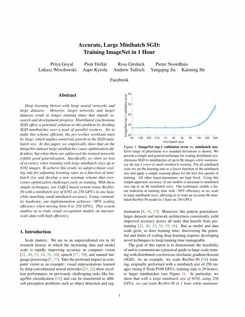
Figure 1. ImageNet top-1 validation error vs. minibatch size.Error range of plus/minus two standard deviations is shown. Wepresent a simple and general technique for scaling distributed syn-chronous SGD to minibatches of up to 8k images while maintain-ing the top-1 error of small minibatch training. For all minibatchsizes we set the learning rate as a linear function of the minibatchsize and apply a simple warmup phase for the first few epochs oftraining. All other hyper-parameters are kept fixed. Using thissimple approach, accuracy of our models is invariant to minibatchsize (up to an 8k minibatch size). Our techniques enable a lin-ear reduction in training time with ∼90% efficiency as we scaleto large minibatch sizes, allowing us to train an accurate 8k mini-batch ResNet-50 model in 1 hour on 256 GPUs.

mentation [8, 10, 27]. Moreover, this pattern generalizes:larger datasets and network architectures consistently yieldimproved accuracy across all tasks that benefit from pre-training [22, 40, 33, 34, 35, 16]. But as model and datascale grow, so does training time; discovering the poten-tial and limits of scaling deep learning requires developingnovel techniques to keep training time manageable.

The goal of this report is to demonstrate the feasibilityof and to communicate a practical guide to large-scale train-ing with distributed synchronous stochastic gradient descent(SGD). As an example, we scale ResNet-50 [16] train-ing, originally performed with a minibatch size of 256 im-ages (using 8 Tesla P100 GPUs, training time is 29 hours),to larger minibatches (see Figure 1). In particular, weshow that with a large minibatch size of 8192, using 256GPUs, we can train ResNet-50 in 1 hour while maintain-

1

ing the same level of accuracy as the 256 minibatch base-line. While distributed synchronous SGD is now common-place, no existing results show that validation accuracy canbe maintained with minibatches as large as 8192 or that suchhigh-accuracy models can be trained in such short time.

To tackle this unusually large minibatch size, we em-ploy a simple and generalizable linear scaling rule to ad-just the learning rate. While this guideline is found in ear-lier work [21, 4], its empirical limits are not well under-stood and informally we have found that it is not widelyknown to the research community. To successfully applythis rule, we present a new warmup strategy, i.e., a strategyof using lower learning rates at the start of training [16], toovercome early optimization difficulties. Importantly, notonly does our approach match the baseline validation error,but also yields training error curves that closely match thesmall minibatch baseline. Details are presented in §2.

Our comprehensive experiments in §5 show that opti-mization difficulty is the main issue with large minibatches,rather than poor generalization (at least on ImageNet), incontrast to some recent studies [20]. Additionally, we showthat the linear scaling rule and warmup generalize to morecomplex tasks including object detection and segmentation[9, 30, 14, 27], which we demonstrate via the recently de-veloped Mask R-CNN [14]. We note that a robust and suc-cessful guideline for addressing a wide range of minibatchsizes has not been presented in previous work.

While the strategy we deliver is simple, its successfulapplication requires correct implementation with respect toseemingly minor and often not well understood implemen-tation details within deep learning libraries. Subtleties in theimplementation of SGD can lead to incorrect solutions thatare difficult to discover. To provide more helpful guidancewe describe common pitfalls and the relevant implementa-tion details that can trigger these traps in §3.

Our strategy applies regardless of framework, butachieving efficient linear scaling requires nontrivial com-munication algorithms. We use the recently open-sourcedCaffe21 deep learning framework and Big Basin GPUservers [24], which operates efficiently using standard Eth-ernet networking (as opposed to specialized network inter-faces). We describe the systems algorithms that enable ourapproach to operate near its full potential in §4.

The practical advances described in this report are help-ful across a range of domains. In an industrial domain,our system unleashes the potential of training visual mod-els from internet-scale data, enabling training with billionsof images per day. In a research domain, we have foundit to simplify migrating algorithms from a single-GPUto a multi-GPU implementation without requiring hyper-parameter search, e.g. in our experience migrating FasterR-CNN [30] and ResNets [16] from 1 to 8 GPUs.

1http://www.caffe2.ai

2. Large Minibatch SGDWe start by reviewing the formulation of Stochastic Gra-

dient Descent (SGD), which will be the foundation of ourdiscussions in the following sections. We consider super-vised learning by minimizing a loss L(w) of the form:

L(w) =1

|X|∑x∈X

l(x,w). (1)

Here w are the weights of a network, X is a labeled trainingset, and l(x,w) is the loss computed from samples x ∈ Xand their labels y. Typically l consists of a prediction loss(e.g., cross-entropy loss) and a regularization loss on w.

Minibatch Stochastic Gradient Descent [31], usually re-ferred to as simply as SGD in recent literature even thoughit operates on minibatches, performs the following update:

wt+1 = wt − η1

n

∑x∈B∇l(x,wt). (2)

Here B is a minibatch sampled from X and n = |B| is theminibatch size. η is the learning rate and t is the iterationindex. Note that in practice we use momentum SGD; wereturn to a discussion of momentum in §3.

2.1. Learning Rates for Large Minibatches

Our goal is to use large minibatches in place of smallminibatches while maintaining training and generalizationaccuracy. This is of particular interest in distributed learn-ing, because it can allow us to scale to multiple workers2 us-ing simple data parallelism without reducing the per-workerworkload and without sacrificing model accuracy.

As we will show in comprehensive experiments, wefound that the following learning rate scaling rule is sur-prisingly effective for a broad range of minibatch sizes:

Linear Scaling Rule: When the minibatch size ismultiplied by k, multiply the learning rate by k.

All other hyper-parameters (weight decay, momentum, etc.)are kept unchanged. As we will show in §5, the above lin-ear scaling rule can help us to not only match the accuracybetween using small and large minibatches, but equally im-portantly, to largely match their training curves.

Interpretation. We present an informal discussion of thelinear scaling rule and why it may be effective. Considera network at iteration t with weights wt, and a sequenceof k minibatches Bj for 0 ≤ j < k each of size n. Wecompare the effect of executing k SGD iterations with smallminibatches Bj and learning rate η versus a single iterationwith a large minibatch ∪jBj of size kn and learning rate η.

2We use the terms ‘worker’ and ‘GPU’ interchangeably in this work, al-though other implementations of a ‘worker’ are possible. ‘Server’ denotesa set of 8 GPUs that does not require communication over a network.

2

According to (2), after k iterations of SGD with learningrate η and a minibatch size of n we have:

wt+k = wt − η1

n

∑j<k

∑x∈Bj

∇l(x,wt+j). (3)

On the other hand, taking a single step with the large mini-batch ∪jBj of size kn and learning rate η yields:

wt+1 = wt − η1

kn

∑j<k

∑x∈Bj

∇l(x,wt). (4)

As expected, the updates differ, and it is unlikely that un-der any condition wt+1 = wt+k. However, if we couldassume ∇l(x,wt) ≈ ∇l(x,wt+j) for j < k, then settingη = kn would yield wt+k ≈ wt+k, and the updates fromsmall and large minibatch SGD would be similar. Note thateven under this strong assumption, we emphasize that thetwo updates can be similar only if we set η = kn.

The above interpretation gives intuition for one casewhere we may hope the linear scaling rule to apply. In ourexperiments with η = kη (and warmup), small and largeminibatch SGD not only result in models with the same fi-nal accuracy, but also, the training curves match closely.Our empirical results suggest that the above approximationmight be valid in large-scale, real-world data.

The assumption that ∇l(x,wt) ≈ ∇l(x,wt+j) oftenmay not hold, and in practice we found the rule does notapply in two cases. First, in the initial training epochs whenthe network is changing rapidly, it does not hold. We ad-dress this by using a warmup phase, discussed in §2.2. Sec-ond, minibatch size cannot be scaled indefinitely: while re-sults are stable for a large range of sizes, beyond a certainpoint accuracy degrades rapidly. Interestingly, this point isas large as ∼8k in ImageNet experiments.

Discussion. The above linear scaling rule was adopted byKrizhevsky [21], if not earlier. However, Krizhevsky re-ported a 1% increase of error when increasing the minibatchsize from 128 to 1024, whereas we show how to maintainaccuracy across a much broader regime of minibatch sizes.Chen et al. [5] presented a comparison of numerous dis-tributed SGD variants, and although their work also em-ployed the linear scaling rule, it did not establish a smallminibatch baseline (the most related result is in v1 of [5]which reported a 0.4% increase of error when the minibatchsize increases from 1600 to 6400 images using synchronousSGD, but results on smaller minibatches are not available).

In their recent review paper, Bottou et al. [4] (section4.2) discuss the theoretical tradeoffs of minibatching andshow that with the linear scaling rule, solvers follow thesame training curve when having seen the same number ofexamples; it also suggests that the learning rate should notexceed a maximum rate that does not depend on the mini-batch size (which justifies warmup). Our work empiricallytests these theories with unprecedented minibatch sizes.

2.2. Warmup

As we discussed, for large minibatches (e.g., 8k) the lin-ear scaling rule breaks down when the network is changingrapidly, which commonly occurs in early stages of train-ing. We find that this issue can be alleviated by a properlydesigned warmup [16], namely, a strategy of using less ag-gressive learning rates at the start of training.

Constant warmup. The warmup strategy presented in [16]uses a low constant learning rate for the first few epochs oftraining. As we will show in §5, we have found constantwarmup particularly helpful for prototyping object detec-tion and segmentation methods [9, 30, 25, 14] that fine-tunepre-trained layers together with newly initialized layers.

In our ImageNet experiments with a large minibatch ofsize kn, we have tried to train with the low learning rate ofη for the first 5 epochs and then return to the target learn-ing rate of η = kη. However, given a large k, we find thatthis constant warmup is not sufficient to solve the optimiza-tion problem, and a transition out of the low learning ratewarmup phase can cause the training error to spike. Thisleads us to propose the following gradual warmup.

Gradual warmup. We present an alternative warmup thatgradually ramps up the learning rate from a small to a largevalue. This ramp avoids a sudden increase from a smalllearning rate to a large one, allowing healthy convergenceat the start of training. In practice, with a large minibatchof size kn, we start from a learning rate of η and incrementit by a constant amount at each iteration such that it reachesη = kη after 5 epochs. After the warmup phase, we go backto the original learning rate schedule.

2.3. Batch Normalization with Large Minibatches

Batch Normalization (BN) [19] computes statistics alongthe minibatch dimension: this breaks the independence ofeach sample’s loss, and changes in minibatch size changethe underlying definition of the loss function being opti-mized. In the following we will show that a commonly used‘shortcut’, which may appear to be a practical considerationto avoid communication overhead, is actually necessary forpreserving the loss function when changing minibatch size.

We note that (1) and (2) assume the per-sample lossl(x,w) is independent of all other samples. This is not thecase when BN is performed and activations are computedacross samples. We write lB(x,w) to denote that the loss ofa single sample x depends on the statistics of all samples inits minibatch B. We denote the loss over a single minibatchB of size n as L(B, w) = 1

n

∑x∈B lB(x,w). With BN, the

training set can be thought of as containing all distinct sub-sets of size n drawn from the original training set X , whichwe denote as Xn. The training loss L(w) then becomes:

L(w) =1

|Xn|∑B∈Xn

L(B, w). (5)

3

If we view B as a ‘single sample’ in Xn, then the loss ofeach single sample B is computed independently.

Note that the minibatch size n over which the BN statis-tics are computed is a key component of the loss: if the per-worker minibatch sample size n is changed, it changes theunderlying loss function L that is optimized. More specif-ically, the mean/variance statistics computed by BN withdifferent n exhibit different random levels of variation.

In the case of distributed (and multi-GPU) training, if theper-worker sample size n is kept fixed and the total mini-batch size is kn, it can be viewed a minibatch of k sampleswith each sample Bj independently selected from Xn, sothe underlying loss function is unchanged and is still de-fined in Xn. Under this point of view, in the BN settingafter seeing k minibatches Bj , (3) and (4) become:

wt+k = wt − η∑j<k

∇L(Bj , wt+j), (6)

wt+1 = wt − η1

k

∑j<k

∇L(Bj , wt). (7)

Following similar logic as in §2.1, we set η = kη and wekeep the per-worker sample size n constant when we changethe number of workers k.

In this work, we use n = 32 which has performed wellfor a wide range of datasets and networks [19, 16]. If n isadjusted, it should be viewed as a hyper-parameter of BN,not of distributed training. We also note that the BN statis-tics should not be computed across all workers, not only forthe sake of reducing communication, but also for maintain-ing the same underlying loss function being optimized.

3. Subtleties and Pitfalls of Distributed SGDIn practice a distributed implementation has many sub-

tleties. Many common implementation errors change thedefinitions of hyper-parameters, leading to models that trainbut whose error may be higher than expected, and such is-sues can be difficult to discover. While the remarks beloware straightforward, they are important to consider explic-itly to faithfully implement the underlying solver.

Weight decay. Weight decay is actually the outcome of thegradient of an L2-regularization term in the loss function.More formally, the per-sample loss in (1) can be written asl(x,w) = λ

2 ‖w‖2 + ε(x,w). Here λ

2 ‖w‖2 is the sample-

independent L2 regularization on the weights and ε(x,w)is a sample-dependent term such as the cross-entropy loss.The SGD update in (2) can be written as:

wt+1 = wt − ηλwt − η1

n

∑x∈B∇ε(x,wt). (8)

In practice, usually only the sample-dependent term∑∇ε(x,wt) is computed by backprop; the term λwt is

computed separately and added to the aggregated gradients

contributed by ε(x,wt). If there is no weight decay term,there are many equivalent ways of scaling the learning rate,including scaling the term ε(x,wt). However, as can beseen from (8), in general this is not the case. We summarizethese observations in the following remark:

Remark 1: Scaling the cross-entropy loss isnot equivalent to scaling the learning rate.

Momentum correction. Momentum SGD is a commonlyadopted modification to the vanilla SGD in (2). A referenceimplementation of momentum SGD has the following form:

ut+1 = mut +1

n

∑x∈B∇l(x,wt)

wt+1 = wt − ηut+1.

(9)

Here m is the momentum decay factor and u is the updatetensor. A popular variant absorbs the learning rate η intothe update tensor. Substituting vt for ηut in (9) yields:

vt+1 = mvt + η1

n

∑x∈B∇l(x,wt)

wt+1 = wt − vt+1.

(10)

For a fixed η, the two are equivalent. However, we note thatwhile u only depends on the gradients and is independentof η, v is entangled with η. When η changes, to maintainequivalence with the reference variant in (9), the update forv should be: vt+1 = mηt+1

ηtvt + ηt+1

1n

∑∇l(x,wt). We

refer to the factor ηt+1

ηtas the momentum correction. We

found that this is especially important for stabilizing train-ing when ηt+1 � ηt, otherwise the history term vt is toosmall which leads to instability (for ηt+1 < ηt momentumcorrection is less critical). This leads to our second remark:

Remark 2: Apply momentum correctionafter changing learning rate if using (10).

Gradient aggregation. For k workers each with a per-worker minibatch of size n, following (4), gradient aggre-gation must be performed over the entire set of kn examplesaccording to 1

kn

∑j

∑x∈Bj

l(x,wt). Loss layers are typi-cally implemented to compute an average loss over their lo-cal input, which amounts to computing a per-worker loss of∑l(x,wt)/n. Given this, correct aggregation requires av-

eraging the k gradients in order to recover the missing 1/kfactor. However, standard communication primitives likeallreduce [11] perform summing, not averaging. Therefore,it is more efficient to absorb the 1/k scaling into the loss,in which case only the loss’s gradient with respect to its in-put needs to be scaled, removing the need to scale the entiregradient vector. We summarize this as follows:

Remark 3: Normalize the per-worker loss bytotal minibatch size kn, not per-worker size n.

We also note that it may be incorrect to ‘cancel k’ by settingη = η (not kη) and normalizing the loss by 1/n (not 1/kn),which can lead to incorrect weight decay (see Remark 1).

4

Data shuffling. SGD is typically analyzed as a process thatsamples data randomly with replacement. In practice, com-mon SGD implementations apply random shuffling of thetraining set during each SGD epoch, which can give betterresults [3, 13]. To provide fair comparisons with baselinesthat use shuffling (e.g., [16]), we ensure the samples in oneepoch done by k workers are from a single consistent ran-dom shuffling of the training set. To achieve this, for eachepoch we use a random shuffling that is partitioned into kparts, each of which is processed by one of the k workers.Failing to correctly implement random shuffling in multipleworkers may lead to noticeably different behavior, whichmay contaminate results and conclusions. In summary:

Remark 4: Use a single random shuffling of the trainingdata (per epoch) that is divided amongst all k workers.

4. Communication

In order to scale beyond the 8 GPUs in a single Big Basinserver [24], gradient aggregation has to span across serverson a network. To allow for near perfect linear scaling, theaggregation must be performed in parallel with backprop.This is possible because there is no data dependency be-tween gradients across layers. Therefore, as soon as the gra-dient for a layer is computed, it is aggregated across work-ers, while gradient computation for the next layer continues(as discussed in [5]). We give full details next.

4.1. Gradient Aggregation

For every gradient, aggregation is done using an allre-duce operation (similar to the MPI collective operationMPI Allreduce [11]). Before allreduce starts every GPU hasits locally computed gradients and after allreduce completesevery GPU has the sum of all k gradients. As the numberof parameters grows and compute performance of GPUs in-creases, it becomes harder to hide the cost of aggregation inthe backprop phase. Training techniques to overcome theseeffects are beyond the scope of this work (e.g., quantizedgradients [18], Block-Momentum SGD [6]). However, atthe scale of this work, collective communication was nota bottleneck, as we were able to achieve near-linear SGDscaling by using an optimized allreduce implementation.

Our implementation of allreduce consists of three phasesfor communication within and across servers: (1) buffersfrom the 8 GPUs within a server are summed into a sin-gle buffer for each server, (2) the results buffers are sharedand summed across all servers, and finally (3) the resultsare broadcast onto each GPU. For the local reduction andbroadcast in phases (1) and (3) we used NVIDIA CollectiveCommunication Library (NCCL)3 for buffers of size 256KB or more and a simple implementation consisting of a

3https://developer.nvidia.com/nccl

number of GPU-to-host memory copies and a CPU reduc-tion otherwise. NCCL uses GPU kernels to accelerate in-traserver collectives, so this approach dedicates more timeon the GPU to backprop while using the CPU resources thatwould otherwise have been idle to improve throughput.

For interserver allreduce, we implemented two of thebest algorithms for bandwidth-limited scenarios: the re-cursive halving and doubling algorithm [29, 36] and thebucket algorithm (also known as the ring algorithm) [2].For both, each server sends and receives 2p−1p b bytes ofdata, where b is the buffer size in bytes and p is the num-ber of servers. While the halving/doubling algorithm con-sists of 2 log2(p) communication steps, the ring algorithmconsists of 2(p − 1) steps. This generally makes the halv-ing/doubling algorithm faster in latency-limited scenarios(i.e., for small buffer sizes and/or large server counts). Inpractice, we found the halving/doubling algorithm to per-form much better than the ring algorithm for buffer sizesup to a million elements (and even higher on large servercounts). On 32 servers (256 GPUs), using halving/doublingled to a speedup of 3× over the ring algorithm.

The halving/doubling algorithm consists of a reduce-scatter collective followed by an allgather. In the first stepof reduce-scatter, servers communicate in pairs (rank 0 with1, 2 with 3, etc.), sending and receiving for different halvesof their input buffers. For example, rank 0 sends the secondhalf of its buffer to 1 and receives the first half of the bufferfrom 1. A reduction over the received data is performed be-fore proceeding to the next step, where the distance to thedestination rank is doubled while the data sent and receivedis halved. After the reduce-scatter phase is finished, eachserver has a portion of the final reduced vector.

This is followed by the allgather phase, which retracesthe communication pattern from the reduce-scatter in re-verse, this time simply concatenating portions of the finalreduced vector. At each server, the portion of the buffer thatwas being sent in the reduce-scatter is received in the all-gather, and the portion that was being received is now sent.

To support non-power-of-two number of servers, weused the binary blocks algorithm [29]. This is a generalizedversion of the halving/doubling algorithm where serversare partitioned into power-of-two blocks and two additionalcommunication steps are used, one immediately after theintrablock reduce-scatter and one before the intrablock all-gather. Non-power-of-two cases have some degree of loadimbalance compared to power-of-two, though in our runswe did not see significant performance degradation.

4.2. Software

The allreduce algorithms described are implemented inGloo4, a library for collective communication. It supports

4https://github.com/facebookincubator/gloo

5

multiple communication contexts, which means no addi-tional synchronization is needed to execute multiple allre-duce instances in parallel. Local reduction and broadcast(described as phases (1) and (3)) are pipelined with inter-server allreduce where possible.

Caffe2 supports multi-threaded execution of the computegraph that represents a training iteration. Whenever there isno data dependency between subgraphs, multiple threadscan execute those subgraphs in parallel. Applying this tobackprop, local gradients can be computed in sequence,without dealing with allreduce or weight updates. Thismeans that during backprop, the set of runnable subgraphsmay grow faster than we can execute them. For subgraphsthat contain an allreduce run, all servers must choose to exe-cute the same subgraph from the set of runnable subgraphs.Otherwise, we risk distributed deadlock where servers areattempting to execute non-intersecting sets of subgraphs.With allreduce being a collective operation, servers wouldtime out waiting. To ensure correct execution we impose apartial order on these subgraphs. This is implemented usinga cyclical control input, where completion of the n-th allre-duce unblocks execution of the (n + c)-th allreduce, withc being the maximum number of concurrent allreduce runs.Note that this number should be chosen to be lower than thenumber of threads used to execute the full compute graph.

4.3. Hardware

We used Facebook’s Big Basin [24] GPU servers forour experiments. Each server contains 8 NVIDIA TeslaP100 GPUs that are interconnected with NVIDIA NVLink.For local storage, each server has 3.2TB of NVMe SSDs.For network connectivity, the servers have a MellanoxConnectX-4 50Gbit Ethernet network card and are con-nected to Wedge100 [1] Ethernet switches.

We have found 50Gbit of network bandwidth sufficientfor distributed synchronous SGD for ResNet-50, per thefollowing analysis. ResNet-50 has approximately 25 mil-lion parameters. This means the total size of parameters is25 · 106 · sizeof(float) = 100MB. Backprop for ResNet-50on a single NVIDIA Tesla P100 GPU takes 120 ms. Giventhat allreduce requires ∼2× bytes on the network comparedto the value it operates on, this leads to a peak bandwidth re-quirement of 200MB/0.125s = 1600MB/s, or 12.8 Gbit/s,not taking into account communication overhead. When weadd a smudge factor for network overhead, we reach a peakbandwidth requirement for ResNet-50 of ∼15 Gbit/s.

As this peak bandwidth requirement only holds duringbackprop, the network is free to be used for different tasksthat are less latency sensitive then aggregation (e.g. readingdata or saving network snapshots) during the forward pass.

5. Main Results and AnalysisOur main result is that we can train ResNet-50 [16] on

ImageNet [32] using 256 workers in one hour, while match-ing the accuracy of small minibatch training. Applying thelinear scaling rule along with a warmup strategy allows us toseamlessly scale between small and large minibatches (upto 8k images) without tuning additional hyper-parametersor impacting accuracy. In the following subsections we:(1) describe experimental settings, (2) establish the effec-tiveness of large minibatch training, (3) perform a deeperexperimental analysis, (4) show our findings generalize toobject detection/segmentation, and (5) provide timings.

5.1. Experimental Settings

The 1000-way ImageNet classification task [32] servesas our main experimental benchmark. Models are trainedon the ∼1.28 million training images and evaluated by top-1 error on the 50,000 validation images.

We use the ResNet-50 [16] variant from [12], noting thatthe stride-2 convolutions are on 3×3 layers instead of on1×1 layers as in [16]. We use Nesterov momentum [28]with m of 0.9 following [12] but note that standard mo-mentum as was used in [16] is equally effective. We use aweight decay λ of 0.0001 and following [16] we do not ap-ply weight decay on the learnable BN coefficients (namely,γ and β in [19]). In order to keep the training objectivefixed, which depends on the BN batch size n as describedin §2.3, we use n = 32 throughout, regardless of the overallminibatch size. As in [12], we compute the BN statisticsusing running average (with momentum 0.9).

All models are trained for 90 epochs regardless of mini-batch sizes. We apply the linear scaling rule from §2.1 anduse a learning rate of η = 0.1 · kn256 that is linear in the mini-batch size kn. With k = 8 workers (GPUs) and n = 32samples per worker, η = 0.1 as in [16]. We call this num-ber (0.1 · kn256 ) the reference learning rate, and reduce it by1/10 at the 30-th, 60-th, and 80-th epoch, similar to [16].

We adopt the initialization of [15] for all convolutionallayers. The 1000-way fully-connected layer is initialized bydrawing weights from a zero-mean Gaussian with standarddeviation of 0.01. We have found that although SGD with asmall minibatch is not sensitive to initialization due to BN,this is not the case for a substantially large minibatch. Addi-tionally we require an appropriate warmup strategy to avoidoptimization difficulties in early training.

For BN layers, the learnable scaling coefficient γ is ini-tialized to be 1, except for each residual block’s last BNwhere γ is initialized to be 0. Setting γ = 0 in the last BN ofeach residual block causes the forward/backward signal ini-tially to propagate through the identity shortcut of ResNets,which we found to ease optimization at the start of training.This initialization improves all models but is particularlyhelpful for large minibatch training as we will show.

6

We use scale and aspect ratio data augmentation [35] asin [12]. The network input image is a 224×224 pixel ran-dom crop from an augmented image or its horizontal flip.The input image is normalized by the per-color mean andstandard deviation, as in [12].

Handling random variation. As models are subject torandom variation in training, we compute a model’s errorrate as the median error of the final 5 epochs. Moreover,we report the mean and standard deviation (std) of the errorfrom 5 independent runs. This gives us more confidence inour results and also provides a measure of model stability.

The random variation of ImageNet models has generallynot been reported in previous work (largely due to resourcelimitations). We emphasize that ignoring random variationmay cause unreliable conclusions, especially if results arefrom a single trial, or the best of many.

Baseline. Under these settings, we establish a ResNet-50baseline using k = 8 (8 GPUs in one server) and n = 32images per worker (minibatch size of kn = 256), as in [16].Our baseline has a top-1 validation error of 23.60% ±0.12.As a reference, ResNet-50 from fb.resnet.torch [12]has 24.01% error, and that of the original ResNet paper [16]has 24.7% under weaker data augmentation.

5.2. Optimization or Generalization Issues?

We establish our main results on large minibatch train-ing by exploring optimization and generalization behaviors.We will demonstrate that with a proper warmup strategy,large minibatch SGD can both match the training curves ofsmall minibatch SGD and also match the validation error.In other words, in our experiments both optimization andgeneralization of large minibatch training matches that ofsmall minibatch training. Moreover, in §5.4 we will showthat these models exhibit good generalization behavior tothe object detection/segmentation transfer tasks, matchingthe transfer quality of small minibatch models.

For the following results, we use k = 256 and n = 32,which results in a minibatch size kn = 8k (we use ‘1k’to denote 1024). As discussed, our baseline has a mini-batch size of kn = 256 and a reference learning rate ofη = 0.1. Applying the linear scaling rule gives η = 3.2as the reference learning rate for our large minibatch runs.We test three warmup strategies as discussed in §2.2: nowarmup, constant warmup with η = 0.1 for 5 epochs,and gradual warmup which starts with η = 0.1 and islinearly increased to η = 3.2 over 5 epochs. All modelsare trained from scratch and all other hyper-parameters arekept fixed. We emphasize that while better results for anyparticular minibatch size could be obtained by optimizinghyper-parameters for that case; our goal is to match er-rors across minibatch sizes by using a general strategy thatavoids hyper-parameter tuning for each minibatch size.

k n kn η top-1 error (%)

baseline (single server) 8 32 256 0.1 23.60 ±0.12no warmup, Figure 2a 256 32 8k 3.2 24.84 ±0.37constant warmup, Figure 2b 256 32 8k 3.2 25.88 ±0.56gradual warmup, Figure 2c 256 32 8k 3.2 23.74 ±0.09

Table 1. Validation error on ImageNet using ResNet-50 (meanand std computed over 5 trials). We compare the small minibatchmodel (kn=256) with large minibatch models (kn=8k) with vari-ous warmup strategies. Observe that the top-1 validation error forsmall and large minibatch training (with gradual warmup) is quiteclose: 23.60% ±0.12 vs. 23.74% ±0.09, respectively.

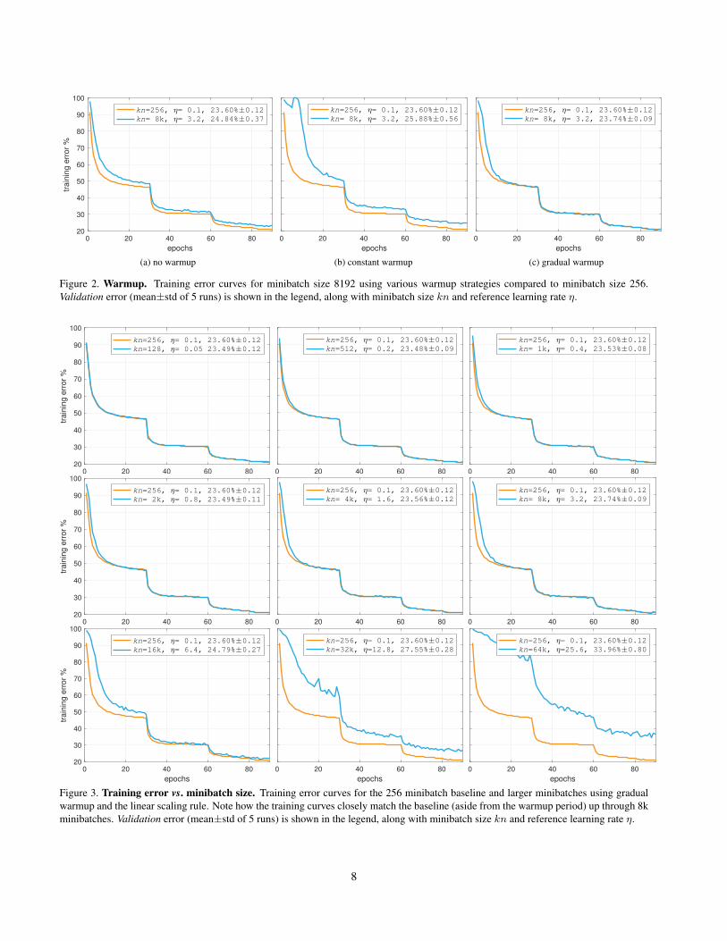
Training error. Training curves are shown in Figure 2.With no warmup (2a), the training curve for large minibatchof kn = 8k is inferior to training with a small minibatch ofkn = 256 across all epochs. A constant warmup strategy(2b) actually degrades results: although the small constantlearning rate can decrease error during warmup, the errorspikes immediately after and training never fully recovers.

Our main result is that with gradual warmup, large mini-batch training error matches the baseline training curve ob-tained with small minibatches, see Figure 2c. Althoughthe large minibatch curve starts higher due to the low ηin the warmup phase, it catches up shortly thereafter. Af-ter about 20 epochs, the small and large minibatch trainingcurves match closely. The comparison between no warmupand gradual warmup suggests that large minibatch sizes arechallenged by optimization difficulties in early training andif these difficulties are addressed, the training error and itscurve can match a small minibatch baseline closely.

Validation error. Table 1 shows the validation error forthe three warmup strategies. The no-warmup variant has∼1.2% higher validation error than the baseline which islikely caused by the ∼2.1% increase in training error (Fig-ure 2a), rather than overfitting or other causes for poor gen-eralization. This argument is further supported by our grad-ual warmup experiment. The gradual warmup variant hasa validation error within 0.14% of the baseline (noting thatstd of these estimates is ∼0.1%). Given that the final train-ing errors (Figure 2c) match nicely in this case, it shows thatif the optimization issues are addressed, there is no apparentgeneralization degradation observed using large minibatchtraining, even if the minibatch size goes from 256 to 8k.

Finally, Figure 4 shows both the training and valida-tion curves for the large minibatch training with gradualwarmup. As can be seen, validation error starts to matchthe baseline closely after the second learning rate drop; ac-tually, the validation curves can match earlier if BN statis-tics are recomputed prior to evaluating the error instead ofusing the running average (see also caption in Figure 4).

7

0 20 40 60 80

epochs

20

30

40

50

60

70

80

90

100

train

ing e

rror

%

kn=256, = 0.1, 23.60% 0.12

kn= 8k, = 3.2, 24.84% 0.37

(a) no warmup

0 20 40 60 80

epochs

kn=256, = 0.1, 23.60% 0.12

kn= 8k, = 3.2, 25.88% 0.56

(b) constant warmup

0 20 40 60 80

epochs

kn=256, = 0.1, 23.60% 0.12

kn= 8k, = 3.2, 23.74% 0.09

(c) gradual warmup

Figure 2. Warmup. Training error curves for minibatch size 8192 using various warmup strategies compared to minibatch size 256.Validation error (mean±std of 5 runs) is shown in the legend, along with minibatch size kn and reference learning rate η.

0 20 40 60 8020

30

40

50

60

70

80

90

100

train

ing e

rror

%

kn=256, = 0.1, 23.60% 0.12

kn=128, = 0.05 23.49% 0.12

0 20 40 60 80

kn=256, = 0.1, 23.60% 0.12

kn=512, = 0.2, 23.48% 0.09

0 20 40 60 80

kn=256, = 0.1, 23.60% 0.12

kn= 1k, = 0.4, 23.53% 0.08

0 20 40 60 8020

30

40

50

60

70

80

90

100

train

ing e

rror

%

kn=256, = 0.1, 23.60% 0.12

kn= 2k, = 0.8, 23.49% 0.11

0 20 40 60 80

kn=256, = 0.1, 23.60% 0.12

kn= 4k, = 1.6, 23.56% 0.12

0 20 40 60 80

kn=256, = 0.1, 23.60% 0.12

kn= 8k, = 3.2, 23.74% 0.09

0 20 40 60 80

epochs

20

30

40

50

60

70

80

90

100

train

ing e

rror

%

kn=256, = 0.1, 23.60% 0.12

kn=16k, = 6.4, 24.79% 0.27

0 20 40 60 80

epochs

kn=256, = 0.1, 23.60% 0.12

kn=32k, =12.8, 27.55% 0.28

0 20 40 60 80

epochs

kn=256, = 0.1, 23.60% 0.12

kn=64k, =25.6, 33.96% 0.80

Figure 3. Training error vs. minibatch size. Training error curves for the 256 minibatch baseline and larger minibatches using gradualwarmup and the linear scaling rule. Note how the training curves closely match the baseline (aside from the warmup period) up through 8kminibatches. Validation error (mean±std of 5 runs) is shown in the legend, along with minibatch size kn and reference learning rate η.

8

0 20 40 60 80

epochs

20

40

60

80

100e

rro

r %

kn=256, =0.1 [train]

kn=256, =0.1 [val]

kn=8k, =3.2 [train]

kn=8k, =3.2 [val]

Figure 4. Training and validation curves for large minibatchSGD with gradual warmup vs. small minibatch SGD. Both setsof curves match closely after training for sufficient epochs. Wenote that the BN statistics (for inference only) are computed us-ing running average, which is updated less frequently with a largeminibatch and thus is noisier in early training (this explains thelarger variation of the validation error in early epochs).

5.3. Analysis Experiments

Minibatch size vs. error. Figure 1 (page 1) shows top-1 validation error for models trained with minibatch sizesranging from of 64 to 65536 (64k). For all models we usedthe linear scaling rule and set the reference learning rateas η = 0.1 · kn256 . For models with kn > 256, we usedthe gradual warmup strategy always starting with η = 0.1and increasing linearly to the reference learning rate after5 epochs. Figure 1 illustrates that validation error remainsstable across a broad range of minibatch sizes, from 64 to8k, after which it begins to increase. Beyond 64k trainingdiverges when using the linear learning rate scaling rule.5

Training curves for various minibatch sizes. Each of thenine plots in Figure 3 shows the top-1 training error curvefor the 256 minibatch baseline (orange) and a second curvecorresponding to different size minibatch (blue). Valida-tion errors are shown in the plot legends. As minibatch sizeincreases, all training curves show some divergence fromthe baseline at the start of training. However, in the caseswhere the final validation error closely matches the base-line (kn ≤ 8k), the training curves also closely match afterthe initial epochs. When the validation errors do not match(kn ≥ 16k), there is a noticeable gap in the training curvesfor all epochs. This suggests that when comparing a newsetting, the training curves can be used as a reliable proxyfor success well before training finishes.

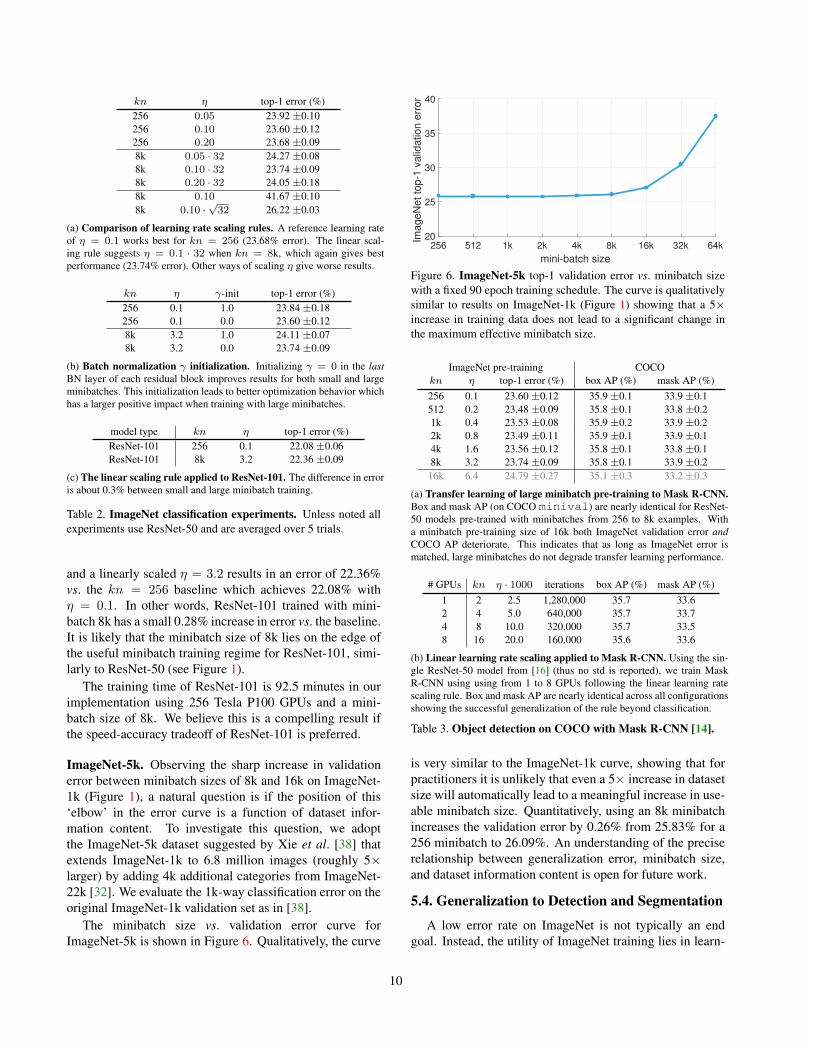
Alternative learning rate rules. Table 2a shows results formultiple learning rates. For small minibatches (kn = 256),

5We note that because of the availability of hardware, we simulated dis-tributed training of very large minibatches (≥12k) on a single server by us-ing multiple gradient accumulation steps between SGD updates. We havethoroughly verified that gradient accumulation on a single server yieldsequivalent results relative to distributed training.

0 20 40 60 80

epochs

20

40

60

80

100

tra

inin

g e

rro

r %

kn=256, = 0.1, 23.60% 0.12

kn=256, = 0.2, 23.68% 0.09

Figure 5. Training curves for small minibatches with differentlearning rates η. As expected, changing η results in curves that donot match. This is in contrast to changing batch-size (and linearlyscaling η), which results in curves that do match, e.g. see Figure 3.

η = 0.1 gives best error but slightly smaller or larger η alsowork well. When applying the linear scaling rule with aminibatch of 8k images, the optimum error is also achievedwith η = 0.1 · 32, showing the successful application of thelinear scaling rule. However, in this case results are moresensitive to changing η. In practice we suggest to use aminibatch size that is not close to the breaking point.

Figure 5 shows the training curves of a 256 minibatchusing η = 0.1 or 0.2. It shows that changing the learningrate η in general changes the overall shapes of the train-ing curves, even if the final error is similar. Contrastingthis result with the success of the linear scaling rule (thatcan match both the final error and the training curves whenminibatch sizes change) may reveal some underlying invari-ance maintained between small and large minibatches.

We also show two alternative strategies: keeping η fixedat 0.1 or using 0.1 ·

√32 according to the square root scaling

rule that was justified theoretically in [21] on grounds that itscales η by the inverse amount of the reduction in the gradi-ent estimator’s standard deviation. For fair comparisons wealso use gradual warmup for 0.1 ·

√32. Both policies work

poorly in practice as the results show.

Batch Normalization γ initialization. Table 2b controlsfor the impact of the new BN γ initialization introduced in§5.1. We show results for minibatch sizes 256 and 8k withthe standard BN initialization (γ = 1 for all BN layers)and with our initialization (γ = 0 for the final BN layerof each residual block). The results show improved per-formance with γ = 0 for both minibatch sizes, and theimprovement is slightly larger for the 8k minibatch size.This behavior also suggests that large minibatches are moreeasily affected by optimization difficulties. We expect thatimproved optimization and initialization methods will helppush the boundary of large minibatch training.

ResNet-101. Results for ResNet-101 [16] are shown in Ta-ble 2c. Training ResNet-101 with a batch-size of kn = 8k

9

kn η top-1 error (%)256 0.05 23.92 ±0.10256 0.10 23.60 ±0.12256 0.20 23.68 ±0.098k 0.05 · 32 24.27 ±0.088k 0.10 · 32 23.74 ±0.098k 0.20 · 32 24.05 ±0.188k 0.10 41.67 ±0.108k 0.10 ·

√32 26.22 ±0.03

(a) Comparison of learning rate scaling rules. A reference learning rateof η = 0.1 works best for kn = 256 (23.68% error). The linear scal-ing rule suggests η = 0.1 · 32 when kn = 8k, which again gives bestperformance (23.74% error). Other ways of scaling η give worse results.

kn η γ-init top-1 error (%)256 0.1 1.0 23.84 ±0.18256 0.1 0.0 23.60 ±0.128k 3.2 1.0 24.11 ±0.078k 3.2 0.0 23.74 ±0.09

(b) Batch normalization γ initialization. Initializing γ = 0 in the lastBN layer of each residual block improves results for both small and largeminibatches. This initialization leads to better optimization behavior whichhas a larger positive impact when training with large minibatches.

model type kn η top-1 error (%)ResNet-101 256 0.1 22.08 ±0.06ResNet-101 8k 3.2 22.36 ±0.09

(c) The linear scaling rule applied to ResNet-101. The difference in erroris about 0.3% between small and large minibatch training.

Table 2. ImageNet classification experiments. Unless noted allexperiments use ResNet-50 and are averaged over 5 trials.

and a linearly scaled η = 3.2 results in an error of 22.36%vs. the kn = 256 baseline which achieves 22.08% withη = 0.1. In other words, ResNet-101 trained with mini-batch 8k has a small 0.28% increase in error vs. the baseline.It is likely that the minibatch size of 8k lies on the edge ofthe useful minibatch training regime for ResNet-101, simi-larly to ResNet-50 (see Figure 1).

The training time of ResNet-101 is 92.5 minutes in ourimplementation using 256 Tesla P100 GPUs and a mini-batch size of 8k. We believe this is a compelling result ifthe speed-accuracy tradeoff of ResNet-101 is preferred.

ImageNet-5k. Observing the sharp increase in validationerror between minibatch sizes of 8k and 16k on ImageNet-1k (Figure 1), a natural question is if the position of this‘elbow’ in the error curve is a function of dataset infor-mation content. To investigate this question, we adoptthe ImageNet-5k dataset suggested by Xie et al. [38] thatextends ImageNet-1k to 6.8 million images (roughly 5×larger) by adding 4k additional categories from ImageNet-22k [32]. We evaluate the 1k-way classification error on theoriginal ImageNet-1k validation set as in [38].

The minibatch size vs. validation error curve forImageNet-5k is shown in Figure 6. Qualitatively, the curve

256 512 1k 2k 4k 8k 16k 32k 64k

mini-batch size

20

25

30

35

40

ImageN

et to

p-1

valid

ation e

rror

Figure 6. ImageNet-5k top-1 validation error vs. minibatch sizewith a fixed 90 epoch training schedule. The curve is qualitativelysimilar to results on ImageNet-1k (Figure 1) showing that a 5×increase in training data does not lead to a significant change inthe maximum effective minibatch size.

ImageNet pre-training COCOkn η top-1 error (%) box AP (%) mask AP (%)256 0.1 23.60 ±0.12 35.9 ±0.1 33.9 ±0.1512 0.2 23.48 ±0.09 35.8 ±0.1 33.8 ±0.21k 0.4 23.53 ±0.08 35.9 ±0.2 33.9 ±0.22k 0.8 23.49 ±0.11 35.9 ±0.1 33.9 ±0.14k 1.6 23.56 ±0.12 35.8 ±0.1 33.8 ±0.18k 3.2 23.74 ±0.09 35.8 ±0.1 33.9 ±0.216k 6.4 24.79 ±0.27 35.1 ±0.3 33.2 ±0.3

(a) Transfer learning of large minibatch pre-training to Mask R-CNN.Box and mask AP (on COCO minival) are nearly identical for ResNet-50 models pre-trained with minibatches from 256 to 8k examples. Witha minibatch pre-training size of 16k both ImageNet validation error andCOCO AP deteriorate. This indicates that as long as ImageNet error ismatched, large minibatches do not degrade transfer learning performance.

# GPUs kn η · 1000 iterations box AP (%) mask AP (%)1 2 2.5 1,280,000 35.7 33.62 4 5.0 640,000 35.7 33.74 8 10.0 320,000 35.7 33.58 16 20.0 160,000 35.6 33.6

(b) Linear learning rate scaling applied to Mask R-CNN. Using the sin-gle ResNet-50 model from [16] (thus no std is reported), we train MaskR-CNN using using from 1 to 8 GPUs following the linear learning ratescaling rule. Box and mask AP are nearly identical across all configurationsshowing the successful generalization of the rule beyond classification.

Table 3. Object detection on COCO with Mask R-CNN [14].

is very similar to the ImageNet-1k curve, showing that forpractitioners it is unlikely that even a 5× increase in datasetsize will automatically lead to a meaningful increase in use-able minibatch size. Quantitatively, using an 8k minibatchincreases the validation error by 0.26% from 25.83% for a256 minibatch to 26.09%. An understanding of the preciserelationship between generalization error, minibatch size,and dataset information content is open for future work.

5.4. Generalization to Detection and Segmentation

A low error rate on ImageNet is not typically an endgoal. Instead, the utility of ImageNet training lies in learn-

10

256 512 1k 2k 4k 8k 11k

mini-batch size

0.2

0.22

0.24

0.26

0.28

0.3

tim

e p

er

itera

tion (

secs)

0.5

1

2

4

8

16

tim

e p

er

epoch (

min

s)

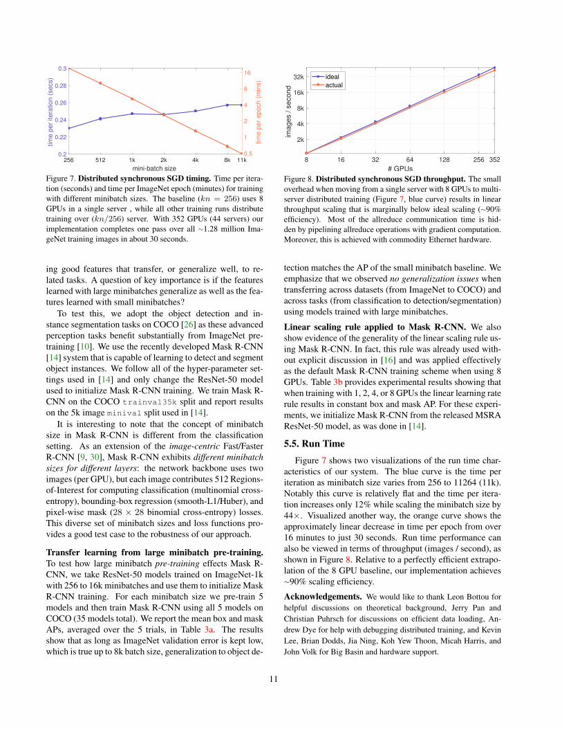
Figure 7. Distributed synchronous SGD timing. Time per itera-tion (seconds) and time per ImageNet epoch (minutes) for trainingwith different minibatch sizes. The baseline (kn = 256) uses 8GPUs in a single server , while all other training runs distributetraining over (kn/256) server. With 352 GPUs (44 servers) ourimplementation completes one pass over all ∼1.28 million Ima-geNet training images in about 30 seconds.

ing good features that transfer, or generalize well, to re-lated tasks. A question of key importance is if the featureslearned with large minibatches generalize as well as the fea-tures learned with small minibatches?

To test this, we adopt the object detection and in-stance segmentation tasks on COCO [26] as these advancedperception tasks benefit substantially from ImageNet pre-training [10]. We use the recently developed Mask R-CNN[14] system that is capable of learning to detect and segmentobject instances. We follow all of the hyper-parameter set-tings used in [14] and only change the ResNet-50 modelused to initialize Mask R-CNN training. We train Mask R-CNN on the COCO trainval35k split and report resultson the 5k image minival split used in [14].

It is interesting to note that the concept of minibatchsize in Mask R-CNN is different from the classificationsetting. As an extension of the image-centric Fast/FasterR-CNN [9, 30], Mask R-CNN exhibits different minibatchsizes for different layers: the network backbone uses twoimages (per GPU), but each image contributes 512 Regions-of-Interest for computing classification (multinomial cross-entropy), bounding-box regression (smooth-L1/Huber), andpixel-wise mask (28 × 28 binomial cross-entropy) losses.This diverse set of minibatch sizes and loss functions pro-vides a good test case to the robustness of our approach.

Transfer learning from large minibatch pre-training.To test how large minibatch pre-training effects Mask R-CNN, we take ResNet-50 models trained on ImageNet-1kwith 256 to 16k minibatches and use them to initialize MaskR-CNN training. For each minibatch size we pre-train 5models and then train Mask R-CNN using all 5 models onCOCO (35 models total). We report the mean box and maskAPs, averaged over the 5 trials, in Table 3a. The resultsshow that as long as ImageNet validation error is kept low,which is true up to 8k batch size, generalization to object de-

8 16 32 64 128 256 352

# GPUs

2k

4k

8k

16k

32k

ima

ge

s /

se

co

nd

ideal

actual

Figure 8. Distributed synchronous SGD throughput. The smalloverhead when moving from a single server with 8 GPUs to multi-server distributed training (Figure 7, blue curve) results in linearthroughput scaling that is marginally below ideal scaling (∼90%efficiency). Most of the allreduce communication time is hid-den by pipelining allreduce operations with gradient computation.Moreover, this is achieved with commodity Ethernet hardware.

tection matches the AP of the small minibatch baseline. Weemphasize that we observed no generalization issues whentransferring across datasets (from ImageNet to COCO) andacross tasks (from classification to detection/segmentation)using models trained with large minibatches.

Linear scaling rule applied to Mask R-CNN. We alsoshow evidence of the generality of the linear scaling rule us-ing Mask R-CNN. In fact, this rule was already used with-out explicit discussion in [16] and was applied effectivelyas the default Mask R-CNN training scheme when using 8GPUs. Table 3b provides experimental results showing thatwhen training with 1, 2, 4, or 8 GPUs the linear learning raterule results in constant box and mask AP. For these experi-ments, we initialize Mask R-CNN from the released MSRAResNet-50 model, as was done in [14].

5.5. Run Time

Figure 7 shows two visualizations of the run time char-acteristics of our system. The blue curve is the time periteration as minibatch size varies from 256 to 11264 (11k).Notably this curve is relatively flat and the time per itera-tion increases only 12% while scaling the minibatch size by44×. Visualized another way, the orange curve shows theapproximately linear decrease in time per epoch from over16 minutes to just 30 seconds. Run time performance canalso be viewed in terms of throughput (images / second), asshown in Figure 8. Relative to a perfectly efficient extrapo-lation of the 8 GPU baseline, our implementation achieves∼90% scaling efficiency.

Acknowledgements. We would like to thank Leon Bottou forhelpful discussions on theoretical background, Jerry Pan andChristian Puhrsch for discussions on efficient data loading, An-drew Dye for help with debugging distributed training, and KevinLee, Brian Dodds, Jia Ning, Koh Yew Thoon, Micah Harris, andJohn Volk for Big Basin and hardware support.

11

References[1] J. Bagga, H. Morsy, and Z. Yao. Opening

designs for 6-pack and Wedge 100. https:

//code.facebook.com/posts/203733993317833/

opening-designs-for-6-pack-and-wedge-100, 2016.[2] M. Barnett, L. Shuler, R. van De Geijn, S. Gupta, D. G.

Payne, and J. Watts. Interprocessor collective communica-tion library (intercom). In Scalable High-Performance Com-puting Conference, 1994.

[3] L. Bottou. Curiously fast convergence of some stochasticgradient descent algorithms. Unpublished open problem of-fered to the attendance of the SLDS 2009 conference, 2009.

[4] L. Bottou, F. E. Curtis, and J. Nocedal. Opt. methods forlarge-scale machine learning. arXiv:1606.04838, 2016.

[5] J. Chen, X. Pan, R. Monga, S. Bengio, and R. Joze-fowicz. Revisiting Distributed Synchronous SGD.arXiv:1604.00981, 2016.

[6] K. Chen and Q. Huo. Scalable training of deep learning ma-chines by incremental block training with intra-block par-allel optimization and blockwise model-update filtering. InICASSP, 2016.

[7] R. Collobert, J. Weston, L. Bottou, M. Karlen,K. Kavukcuoglu, and P. Kuksa. Natural language pro-cessing (almost) from scratch. JMLR, 2011.

[8] J. Donahue, Y. Jia, O. Vinyals, J. Hoffman, N. Zhang,E. Tzeng, and T. Darrell. Decaf: A deep convolutional acti-vation feature for generic visual recognition. In ICML, 2014.

[9] R. Girshick. Fast R-CNN. In ICCV, 2015.[10] R. Girshick, J. Donahue, T. Darrell, and J. Malik. Rich fea-

ture hierarchies for accurate object detection and semanticsegmentation. In CVPR, 2014.

[11] W. Gropp, E. Lusk, and A. Skjellum. Using MPI: PortableParallel Programming with the Message-Passing Interface.MIT Press, Cambridge, MA, 1999.

[12] S. Gross and M. Wilber. Training and investigating Resid-ual Nets. https://github.com/facebook/fb.resnet.torch, 2016.

[13] M. Gurbuzbalaban, A. Ozdaglar, and P. Parrilo. Whyrandom reshuffling beats stochastic gradient descent.arXiv:1510.08560, 2015.

[14] K. He, G. Gkioxari, P. Dollar, and R. Girshick. Mask R-CNN. arXiv:1703.06870, 2017.

[15] K. He, X. Zhang, S. Ren, and J. Sun. Delving deep intorectifiers: Surpassing human-level performance on imagenetclassification. In ICCV, 2015.

[16] K. He, X. Zhang, S. Ren, and J. Sun. Deep residual learningfor image recognition. In CVPR, 2016.

[17] G. Hinton, L. Deng, D. Yu, G. E. Dahl, A.-r. Mohamed,N. Jaitly, A. Senior, V. Vanhoucke, P. Nguyen, T. N. Sainath,et al. Deep neural networks for acoustic modeling in speechrecognition: The shared views of four research groups. IEEESignal Processing Magazine, 2012.

[18] I. Hubara, M. Courbariaux, D. Soudry, R. El-Yaniv, andY. Bengio. Quantized neural networks: Training neu-ral networks with low precision weights and activations.arXiv:1510.08560, 2016.

[19] S. Ioffe and C. Szegedy. Batch normalization: Acceleratingdeep network training by reducing internal covariate shift. InICML, 2015.

[20] N. S. Keskar, D. Mudigere, J. Nocedal, M. Smelyanskiy, andP. T. P. Tang. On large-batch training for deep learning: Gen-eralization gap and sharp minima. ICLR, 2017.

[21] A. Krizhevsky. One weird trick for parallelizing convolu-tional neural networks. arXiv:1404.5997, 2014.

[22] A. Krizhevsky, I. Sutskever, and G. Hinton. ImageNet classi-fication with deep convolutional neural nets. In NIPS, 2012.

[23] Y. LeCun, B. Boser, J. S. Denker, D. Henderson, R. E.Howard, W. Hubbard, and L. D. Jackel. Backpropagationapplied to handwritten zip code recognition. Neural compu-tation, 1989.

[24] K. Lee. Introducing Big Basin: Our next-generationAI hardware. https://code.facebook.com/posts/

1835166200089399/introducing-big-basin, 2017.[25] T.-Y. Lin, P. Dollar, R. Girshick, K. He, B. Hariharan, and

S. Belongie. Feature pyramid networks for object detection.In CVPR, 2017.

[26] T.-Y. Lin, M. Maire, S. Belongie, J. Hays, P. Perona, D. Ra-manan, P. Dollar, and C. L. Zitnick. Microsoft COCO: Com-mon objects in context. In ECCV. 2014.

[27] J. Long, E. Shelhamer, and T. Darrell. Fully convolutionalnetworks for semantic segmentation. In CVPR, 2015.

[28] Y. Nesterov. Introductory lectures on convex optimization: Abasic course. Springer, 2004.

[29] R. Rabenseifner. Optimization of collective reduction oper-ations. In ICCS. Springer, 2004.

[30] S. Ren, K. He, R. Girshick, and J. Sun. Faster R-CNN: To-wards real-time object detection with region proposal net-works. In NIPS, 2015.

[31] H. Robbins and S. Monro. A stochastic approximationmethod. The annals of mathematical statistics, 1951.

[32] O. Russakovsky, J. Deng, H. Su, J. Krause, S. Satheesh,S. Ma, Z. Huang, A. Karpathy, A. Khosla, M. Bernstein,A. C. Berg, and L. Fei-Fei. ImageNet Large Scale VisualRecognition Challenge. IJCV, 2015.

[33] P. Sermanet, D. Eigen, X. Zhang, M. Mathieu, R. Fergus,and Y. LeCun. Overfeat: Integrated recognition, localizationand detection using convolutional networks. In ICLR, 2014.

[34] K. Simonyan and A. Zisserman. Very deep convolutionalnetworks for large-scale image recognition. In ICLR, 2015.

[35] C. Szegedy, W. Liu, Y. Jia, P. Sermanet, S. Reed,D. Anguelov, D. Erhan, V. Vanhoucke, and A. Rabinovich.Going deeper with convolutions. In CVPR, 2015.

[36] R. Thakur, R. Rabenseifner, and W. Gropp. Optimization ofcollective comm. operations in MPICH. IJHPCA, 2005.

[37] Y. Wu, M. Schuster, Z. Chen, Q. V. Le, M. Norouzi,W. Macherey, M. Krikun, Y. Cao, Q. Gao, K. Macherey,et al. Google’s neural machine translation system: Bridg-ing the gap between human and machine translation.arXiv:1609.08144, 2016.

[38] S. Xie, R. Girshick, P. Dollar, Z. Tu, and K. He. Aggregatedresidual transformations for deep neural networks. In CVPR,2017.

[39] W. Xiong, J. Droppo, X. Huang, F. Seide, M. Seltzer, A. Stol-cke, D. Yu, and G. Zweig. The Microsoft 2016 Conversa-tional Speech Recognition System. arXiv:1609.03528, 2016.

[40] M. D. Zeiler and R. Fergus. Visualizing and understandingconvolutional neural networks. In ECCV, 2014.

12