Tiny ImageNet Visual Recognition Challenge

Ya LeDepartment of Statistics

Stanford Universityyle@stanford.edu

Xuan YangDepartment of Electrical Engineering

Stanford Universityxuany@stanford.edu

Abstract

In this work, we investigate the effect of convolutionalnetwork depth, receptive field size, dropout layers, recti-fied activation unit type and dataset noise on its accuracy inTiny-ImageNet Challenge settings. In order to make a thor-ough evaluation of the cause of the peformance improve-ment, we start with a basic 5 layer model with 5×5 convo-lutional receptive fields. We keep increasing network depthor reducing receptive field size, and continue applying mod-ern techniques, such as PReLu and dropout, to the model.Our model achieves excellent performance even comparedto state-of-the-art results, with 0.444 final error rate on thetest set.

1. IntroductionConvolutional neural networks have demonstrated

recognition accuracy better than or comparable to humansin several visual recognition tasks, including recognizingtraffic signs, faces, and handwritten digits. In particular,an important role in the advance of deep visual recognitionarchitectures has been played by the ImageNet Large-ScaleVisual Recognition Challenge (ILSVRC) [12], which hasserved as a testbed for a few generations of large-scale im-age classification systems.

In this project, we work on the Tiny ImageNet VisualRecognition Challenge. This challenge runs similar to theImageNet Challenge (ILSVRC). The goal of the challengeis to do as well as possible on the Image Classification prob-lem. The performance is measured by the test set error rate,the fraction of test images that are incorrectly classified bythe model.

We experiment with various convolutional neural net-works, which differ in depth, receptive field size, nonlin-earity layer and number of dropout layers. Our results showthat deeper networks with smaller receptive fields and largernumber of channels usually perform better. Some of ournetworks achieve excellent performance even compared tostate-of-the-art results.

The rest of the paper is organised as follows. We dis-cuss relevant literature in Section 2 and describe our prob-lem and data set in Section 3. The details of our technicalapproaches are presented in Section 4. In Section 5, wedescribe our convolutional neural network configurations,implementation details and experiment results. Section 6concludes the paper.

2. Related Work

Recently there have been tremendous improvements inrecognition performance, mainly due to advances in twotechnical directions: building more powerful models, anddesigning effective strategies against overfitting.

Neural networks are becoming more capable of fittingtraining data. This is majorly due to the development of thefollowing areas: sophisticated layer designs [17, 4]; newnonlinear activations [11, 10, 20, 16, 3, 5]; and increasedcomplexity, including increased depth [17, 14], enlargedwidth [19, 13], and the use of smaller strides [19, 13, 1, 14].

Since networks are more complex, it’s necessary to havebetter strategies for model generalization. This is achievedby large-scale data [2, 12], aggressive data augmentation[9, 7, 14, 17], and effective regularization techniques [6, 15,3, 18].

3. Problem Statement

The goal of this challenge is to estimate the content ofphotographs for the purpose of retrieval and automatic an-notation using a subset of the large hand-labeled ImageNetdataset (10,000,000 labeled images depicting 10,000+ ob-ject categories) as training. Test images will be presentedwith no initial annotation – no segmentation or labels –and algorithms will have to produce labelings specifying towhich category the images belong. New test images arecollected and labeled especially for the original ImageNetChallenge and are not part of the previously published Im-ageNet dataset. The general goal is to identify the mainobjects present in images and to make image classification.

1

3.1. Data

The TinyImageNet dataset is a subset of the ILSVRC-2012 classification dataset. It consists of 200 object classes,and for each object class it provides 500 training images,50 validation images, and 50 test images. All images havebeen downsampled to 64× 64× 3 pixels. The training andvalidation sets are released with images and annotations, in-cluding both class labels and bounding boxes. But the maingoal of this project is to predict the class label of each im-age without localizing the objects. The test set is releasedwithout labels or bounding boxes.

3.2. Evaluation

For each image, algorithms will produce one label whichhas largest estimated probability. The quality of a labelingwill be evaluated based on the ground truth label for theimage. The error of the algorithm for that image would be 1if the predicted label doesn’t match the ground truth label,and 0 otherwise. The overall error score for an algorithm isthe average error over all test images.

4. Technical Approach

4.1. Model Architecture

In the last few years, mainly due to the advances of deeplearning, more concretely convolutional networks, the qual-ity of image recognition and object detection has been pro-gressing at a dramatic pace. Therefore we will focus on adeep neural network architecture for this project. We willexperiment with the following architectures with severaldropout layers inserted in the network and use the valida-tion set to tune the hyperparameters, including filter size,number of filters, network depth, learning rate and regular-ization strength, etc.

1. [conv-relu-pool]×N - conv - relu - [affine]×M - [soft-max or SVM]

2. [conv-relu-pool]×N - [affine]×M - [softmax or SVM]

3. [conv-relu-conv-relu-pool]×N - [affine]×M - [soft-max or SVM]

4.2. Reduce Overfitting

Since there are only 500 training images for eachclass, which is a much smaller training set compared tothe ILSVRC-2012 classification dataset, it’s insufficient tolearn a deep neural network without considerable overfit-ting. We consider the following two primary ways to reduceoverfitting.

4.2.1 Data Augmentation

The easiest and most common method to reduce overfit-ting on image data is to artificially enlarge the dataset us-ing label-preserving transformations. We will employ fourdistinct forms of data augmentation at training time, all ofwhich allow transformed images to be produced from theoriginal images with very little computation, so the trans-formed images do not need to be stored on disk. At trainingphase, the network random choose from ten transformedimages of the given test image, which are the four cornercrops and the center crop, as well as their horizontal reflec-tions. At test time, the network makes a prediction based onthe center crop.

1. Random crops. The images of Tiny ImageNet Chal-lenge are 64× 64× 3. Instead of feeding our trainingimages directly to the convnet, at training time we willrandomly crop each training image to 56× 56× 3 andtrain our network on these extracted crops.

2. Random flips. We will randomly flip half of the train-ing images horizontally.

4.2.2 Dropout

The recently-introduced technique ”dropout” [15] is a veryefficient version of model combination that only costs abouta factor of two during training. While training, dropout isimplemented by only keeping a neuron active with someprobability p, or setting it to zero otherwise. At test time,we will use all the neurons but multiply their outputs by p.

Since the dropped-out neurons do not contribute to theforward pass and do not participate in back-propagation, theneural network samples a different architecture every timean input is presented, while all these architectures shareweights. In this way, a neuron cannot rely on the presenceof particular other neurons. Therefore, the droput techniquereduces complex co-adaptations of neurons, and is forcedto learn more robust features that are useful in conjunctionwith many different random subsets of the other neurons.

For this project, we will use the inverted dropout, whichperforms the scaling at train time, leaving the forward passat test time untouched, with p = 0.5.

4.3. Other Techniques

4.3.1 Model Ensemble

One reliable approach to improving the performance ofNeural Networks is to train multiple independent models,and at test time average their predictions. Usually the im-provements are more dramatic with higher model variety inthe ensemble. We will use the following two ways to forman ensemble. Using which one will depend on the complex-ity of the network.

2

1. Top models discovered during cross-validation. Wewill use cross-validation to determine the best hyper-parameters, then pick the top few models to formthe ensemble. This can be easier to perform since itdoesn’t require additional retraining of models aftercross-validation.

2. Different checkpoints of a single model. For complexnetworks which are expensive to train, we will takedifferent checkpoints of a single network over time anduse those to form an ensemble.

4.3.2 Parametric Rectifiers

We will experiment with the network that replaces theparameter-free ReLU activation by a learned parametric ac-tivation, called Parametric Rectified Linear Unit (PReLU)[5]. This activation function adaptively learns the param-eters of the rectifiers, and improves accuracy at negligibleextra computational cost.

Formally, the activation function is defined as f(yi) =max(0, yi)+ai min(0, yi), where yi is the input of the non-linear activation f on the ith channel, and ai is a coefficientcontrolling the slope of the negative part, which allows thenonlinear activation to vary on different channels. If ai = 0,it becomes ReLU; if ai is a small and fixed value, PReLUbecomes the Leaky ReLU (LReLU) in [10]. The number ofextra parameters that PReLu introduces is equal to the totalnumber of channels, which is negligible when consideringthe total number of weights.

5. Experiment

5.1. Model Configuration

We experiment with nine different models. The config-urations of these convolutional neural networks and theirnumber of parameters are outlined in Table 1, one per col-umn. Particularly, Model 9 is inspired by VGG model [14]and modified to fit our dataset. These model configurationsdiffer in the following ways:

1. Depth: The depth ranges from 5 layers in Model 1 to16 layers in Model 9.

2. Receptive field size: Most conv layers in Model 1-4have 5 × 5 receptive fields, while all conv layers inModel 5-9 use 3× 3 receptive fields.

3. Number of kernels: The number of kernels rangesfrom 128 in Model 1 to 512 in Model 9.

4. Dropout. As the neural net gets deeper, we add moredropout layers.

5. ReLU layer: Each convoluational layer in Model 1-4and Model 9 is followed by a ReLU layer, while con-volutional layer in Model 5 is followed by a PReLUlayer, and each convolutional layer in Model 6-8 is fol-lowed by a LReLu layer.

5.2. Implementation Details

We implemented our models using the publicly availableC++ Caffe toolbox [8] on GPUs provided Amazon Web Ser-vices. We modified the caffe code to add PLeRu layers (andLReLu is just a special case of PReLU). Here we focus onthe implementation details of Model 8 and Model 9 as thesetwo models have the best performances and they are evalu-ated on the test set.

5.2.1 Training Methodology

The training is carried out by minimizing the regularizedmultinomial logistic regression loss using mini-batch gra-dient descent with momentum. All the training images arerandomly cropped to 56× 56× 3 images.

The original Imagenet Challenge has input dataset as224x224, but the Tiny Imagenet Challenge only has inputsize 64x64. With cropping the input image, some objectsare located in the corner. During data augmentation, withrandom crop, the object will be even further away from thecenter of our view, or even outside the crop. This makesthe image become an invalide training data, and we need toeliminate them from the training dataset. With the providedobject bounding box, this becomes feasible. We check theobject location of each image, if less than 1/4 of the object isa random crop, we will remove the image from the dataset.Specifically, Model 1-4 are trained using all training im-ages, while Model 5-9 are trained using screened images.

For all of our models, the batch size was set to 200, mo-mentum to 0.9 and dropout ratio to 0.5. The learning ratewas initially set to 0.02 for Model 8 and 0.01 for Model 9,and then decreased by a factor of 0.1 and 10 respectivelywhen the validation set accuracy stopped improving. Theweight decay (the L2 penalty multiplier) was set to 1×10−4

for Model 8 and 5× 10−4 for Model 9.For deep networks, it’s important to have good initializa-

tions due to the non-convexity of the learning objective. Weadopted the training strategy in [14], where we began withtraining first few convolutional layers and the last three fullyconnected layers so that the network is shallow enough tobe trained with random initialisation. Then we initialisedthe first few convolutional layers and the last three fullyconnected layers with the weights derived from previoustraining, and initialised the intermediate layers randomly.For random initialisation, we use the caffe xavier algorithmto fill weights, which automatically determines the scale of

3

Table 1. ConvNet configurations (shown in columns). The depth of the configurations increases from the left (Model 1) to the right(Model 9), as more layers are added. The convolutional layer parameters are denoted as conv (receptive field size)-number of channels.The ReLU activation function is not shown for brevity.

Input Size Model 1 Model 2 Model 3 Model 4 Model 5 Model 6 Model 7 Model 8 Model 9

56

conv5-64 conv5-64 conv5-64 conv5-64 conv3-64 conv3-64 conv3-128 conv3-128 conv3-64

conv3-64 conv3-64 conv5-64 conv3-64 conv3-64 conv3-128 conv3-128 conv3-64

maxpool

28

conv5-64 conv5-128 conv5-128 conv5-128 conv3-128 conv3-128 conv3-256 conv3-256 conv3-128

conv3-128 conv3-128 conv3-128 conv3-128 conv3-128 conv3-256 conv3-256 conv3-128

dropout

maxpool

14

conv5-128 conv3-256 conv3-256 conv3-256 conv3-256 conv3-256 conv3-512 conv3-512 conv3-256

conv3-256 conv3-256 conv3-256 conv3-256 conv3-512 conv3-512 conv3-256

conv3-256

dropout dropout dropout dropout

maxpool

7 six conv3-512 layers

FC1256 1024 1024 1024 1024 1024 2048 2048 4096

dropout

FC22048 2048 4096

dropout dropout dropout

FC3200

softmax

depth (conv+fc) 5 7 8 8 8 8 9 9 16

parameters (M) 1.97 13.74 14.33 14.33 14.20 14.20 60.56 60.56 138

initialization based on the number of input and output neu-rons, and we simply initialize the bias as 0.

5.2.2 Testing Methodology

At test time, the test image is cropped from center to size56×56×3 without any flipping. The trained convolutionalneural network is then applied to the cropped image to ob-tain the soft-max class posteriors for the image.

5.3. Results

We perform the experiments on the 200-class Tiny-ImageNet. The results are measured by top-1 error rate. Weonly use the provided data for training. All the results areevaluated on the validation set, except for the final results,which is evaluated on test set. The validation accuracy islisted in Table 2, and the final accuracy of the ensemblemodel on the test set is 0.556.

5.3.1 Comparison between Dropouts

In Table 2, we compare the effects of adding dropout lay-ers. We used one dropout layer in Model 3, but two dropoutlayers in Model 4. We can see that there is more than 1%top-1 accuracy improvement. The improvement is mainlybecause the dropout layers can help reduce overfitting. Thedifference bewteen training loss and testing loss is smaller

Table 2. Convolutional neural network performance on vali-dation set.

Model Name Depth Nonlinear Screen Val Accuracy (%)

Model 1 5 ReLu N 37.27

Model 2 7 ReLu N 28.20

Model 3 8 ReLu N 38.29

Model 4 8 ReLu N 39.55

Model 5 8 PReLu Y 29.00

Model 6 8 LReLu Y 40.19

Model 7 9 LReLu Y 42.07

Model 8 9 LReLu Y 46.45

Model 9 16 ReLu Y 59.50

Ensemble Model 8+Model 9 Y 61.23

for Model 4 than Model 3, which confirms the regulariza-tion effect of dropout.

5.3.2 Comparison between ReLU, LReLU and PReLU

We implemented Parametric ReLU in caffe and used it inmodel 5, whose network architecture is the same as that ofmodel 4 except that model 4 uses ReLU. Results in Table2 show that parametric ReLU does not help to improve theaccuracy. The reason could be that PReLu introduces moreparameters in the model, resulting in an even worse overfit-ting.

4

Since PReLU does not work well in our case, we replaceReLU with LReLU and set the slope to 0.01. ComparingModel 6 with Model 3, or Model 7 with Model 4, we cansee there is around 2% accuracy improvement. But this im-provement may also result from smaller receptive fields ortraining data screening.

5.3.3 Comparison between Screening Dataset Results

When the object only has less than 1/4 part in a randomcrop, we treat this image as noise in the dataset. With filter-ing out this kind of images, we get a slightly performanceimprovement. The improvement is smaller than we ex-pected mainly due to two reasons. One is we only removed1535 images whose object is at the corner. And statisticsshow that beside those invalide images we still have 1891images whose object area is smaller than 8×8. In this case,it will also be difficult for human to see, but we have not fil-ter those images out. The other reason is that many images,whose object is at corner or small, are in the same class suchas basketball. If we remove all of them from the dataset, itwill also drop the classification peformance for that class.Due to this trade-off, we did not remove the images that hassmall objects. And we see only a small accuracy increase.

5.3.4 Comparision between Single-model Results

Next we compare single-model results. We start with a ba-sic 5 layer model, and track three directions: increasing ker-nel numbers, reducing kernel window and increasing net-work depth. Comparing model 1 with model 3 or model 4,the only difference is we increase the network depth, and wesee around 2% accuracy improvement. However, increasingnetwork depth does not always make peformence between,for example, model 2 get higher error rate.

With more smaller kenel window, we see around 2% ac-curacy improvement by comparing model 3 with model 6or model 4 with model 7. But this improvement may alsocomes with LReLU and screening dataset.

With more kernels and adding another fully-connectedlayer, we see more than 4% accuracy improvement if wecompare model 7 with model 8. However, it needs muchlarger number of parameters and takes longer to train.

5.3.5 Comparision between Multi-model Results

We ensembled the Model 8 and Model 9 in Table 2. For thetime being we have only one model for each architectrue,except architecture 3, we have two models based on differ-ent regularization. Since the last few models such as model8 are much better than the smaller network such as model1, the smaller network does not contribute to the ensembledresult. We tried with ensembling all the models, and get val-idation accuracy as 0.54, but with combining Model 8 and

Figure 1. t-SNE graph for 50 classes of validation set using model9.

Model 9, we get 0.61 validation accuracy. This indicatesthat combining few stronger models is better than combin-ing more poor models. The multi-model accuracy on thetest set is 0.556.

5.4. Visualization

We visualize the classification of our model 9 by extract-ing the feature output of the second fullu-connected layerand plot in t-SNE graph. In t-SNE, the points with the samecolor belongs to the same class. If a certain cluster is fur-ther away from other points in the graph, the network ismore certain about this group of points belong to a certainclass. From Figure 1, we can see, most points are clusteredwell, except for a few points in the center. This implies wehave a decent classification accuracy of model 9.

5.5. Error Analysis

While our results get close to state-of-the-art convolu-tional neural network performance, we still get some mis-classifications shown in Figure 2. Some missclassificationis because some objects have similar shapes, for example,in the first row of Figure 2, the first image (val 1153) showsa vestment, but has been recoginized as alp, and the secondimage(val 4311) is a bucket or pail, but has been classifiedas frying pan. Since convolutional neural networks are verysensitive to texture rather than shape, we are not surprisedto see this kind of miss classification. There are some othermiss classification that are resulted in image down-samplingor crop shown in the second row of Figure 2, such as the firstimage(val 7570) in that row is moving van, but has beenrecoginazed as pop bottle, and the second image(val 8160)is lawn mower, but has been predicted as alp, and we foundeven human feel hard for this kind of images.

5

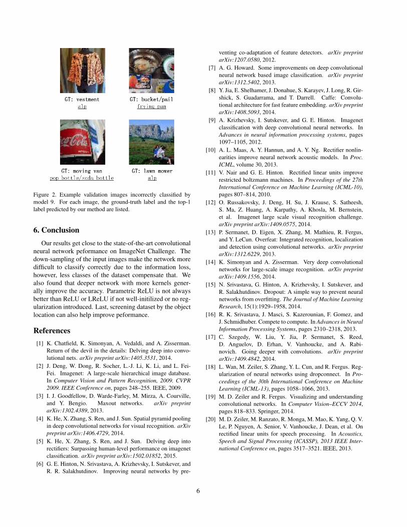
Figure 2. Example validation images incorrectly classified bymodel 9. For each image, the ground-truth label and the top-1label predicted by our method are listed.

6. ConclusionOur results get close to the state-of-the-art convolutional

neural network peformance on ImageNet Challenge. Thedown-sampling of the input images make the network moredifficult to classify correctly due to the information loss,however, less classes of the dataset compensate that. Wealso found that deeper network with more kernels gener-ally improve the accuracy. Parametric ReLU is not alwaysbetter than ReLU or LReLU if not well-initilized or no reg-ularization introduced. Last, screening dataset by the objectlocation can also help improve peformance.

References[1] K. Chatfield, K. Simonyan, A. Vedaldi, and A. Zisserman.

Return of the devil in the details: Delving deep into convo-lutional nets. arXiv preprint arXiv:1405.3531, 2014.

[2] J. Deng, W. Dong, R. Socher, L.-J. Li, K. Li, and L. Fei-Fei. Imagenet: A large-scale hierarchical image database.In Computer Vision and Pattern Recognition, 2009. CVPR2009. IEEE Conference on, pages 248–255. IEEE, 2009.

[3] I. J. Goodfellow, D. Warde-Farley, M. Mirza, A. Courville,and Y. Bengio. Maxout networks. arXiv preprintarXiv:1302.4389, 2013.

[4] K. He, X. Zhang, S. Ren, and J. Sun. Spatial pyramid poolingin deep convolutional networks for visual recognition. arXivpreprint arXiv:1406.4729, 2014.

[5] K. He, X. Zhang, S. Ren, and J. Sun. Delving deep intorectifiers: Surpassing human-level performance on imagenetclassification. arXiv preprint arXiv:1502.01852, 2015.

[6] G. E. Hinton, N. Srivastava, A. Krizhevsky, I. Sutskever, andR. R. Salakhutdinov. Improving neural networks by pre-

venting co-adaptation of feature detectors. arXiv preprintarXiv:1207.0580, 2012.

[7] A. G. Howard. Some improvements on deep convolutionalneural network based image classification. arXiv preprintarXiv:1312.5402, 2013.

[8] Y. Jia, E. Shelhamer, J. Donahue, S. Karayev, J. Long, R. Gir-shick, S. Guadarrama, and T. Darrell. Caffe: Convolu-tional architecture for fast feature embedding. arXiv preprintarXiv:1408.5093, 2014.

[9] A. Krizhevsky, I. Sutskever, and G. E. Hinton. Imagenetclassification with deep convolutional neural networks. InAdvances in neural information processing systems, pages1097–1105, 2012.

[10] A. L. Maas, A. Y. Hannun, and A. Y. Ng. Rectifier nonlin-earities improve neural network acoustic models. In Proc.ICML, volume 30, 2013.

[11] V. Nair and G. E. Hinton. Rectified linear units improverestricted boltzmann machines. In Proceedings of the 27thInternational Conference on Machine Learning (ICML-10),pages 807–814, 2010.

[12] O. Russakovsky, J. Deng, H. Su, J. Krause, S. Satheesh,S. Ma, Z. Huang, A. Karpathy, A. Khosla, M. Bernstein,et al. Imagenet large scale visual recognition challenge.arXiv preprint arXiv:1409.0575, 2014.

[13] P. Sermanet, D. Eigen, X. Zhang, M. Mathieu, R. Fergus,and Y. LeCun. Overfeat: Integrated recognition, localizationand detection using convolutional networks. arXiv preprintarXiv:1312.6229, 2013.

[14] K. Simonyan and A. Zisserman. Very deep convolutionalnetworks for large-scale image recognition. arXiv preprintarXiv:1409.1556, 2014.

[15] N. Srivastava, G. Hinton, A. Krizhevsky, I. Sutskever, andR. Salakhutdinov. Dropout: A simple way to prevent neuralnetworks from overfitting. The Journal of Machine LearningResearch, 15(1):1929–1958, 2014.

[16] R. K. Srivastava, J. Masci, S. Kazerounian, F. Gomez, andJ. Schmidhuber. Compete to compute. In Advances in NeuralInformation Processing Systems, pages 2310–2318, 2013.

[17] C. Szegedy, W. Liu, Y. Jia, P. Sermanet, S. Reed,D. Anguelov, D. Erhan, V. Vanhoucke, and A. Rabi-novich. Going deeper with convolutions. arXiv preprintarXiv:1409.4842, 2014.

[18] L. Wan, M. Zeiler, S. Zhang, Y. L. Cun, and R. Fergus. Reg-ularization of neural networks using dropconnect. In Pro-ceedings of the 30th International Conference on MachineLearning (ICML-13), pages 1058–1066, 2013.

[19] M. D. Zeiler and R. Fergus. Visualizing and understandingconvolutional networks. In Computer Vision–ECCV 2014,pages 818–833. Springer, 2014.

[20] M. D. Zeiler, M. Ranzato, R. Monga, M. Mao, K. Yang, Q. V.Le, P. Nguyen, A. Senior, V. Vanhoucke, J. Dean, et al. Onrectified linear units for speech processing. In Acoustics,Speech and Signal Processing (ICASSP), 2013 IEEE Inter-national Conference on, pages 3517–3521. IEEE, 2013.

6