Embed Size (px)
Citation preview

Abrasive wear of hard faced ground engaging tools
DAVID EUGENIO CANTU GOMEZ
Master of Science Thesis
Stockholm, Sweden 2017


Abrasive wear of hard faced ground
engaging tools
David Eugenio Cantú Gómez
Master of Science Thesis MMK 2017:193 MKN 202
KTH Industrial Engineering and Management
Machine Design
SE-100 44 Stockholm

2
1
Examensarbete MMK 2017:193 MKN 202
Abrasiv nötning av ythärdade jordbearbetningsverktyg
David Eugenio Cantú Gómez
Godkänt
2017-10-31
Examinator
Ulf Sellgren
Handledare
Stefan Björklund
Uppdragsgivare
Senad Dizdar
Kontaktperson
Senad Dizdar
SAMMANFATTNING
Jordbearbetningsverktyg är väldigt viktiga komponenter i maskiner för jordbruksapplikationer,
såsom jordbearbetning. Det är skärbladet på plogen, den så kallade plogbillen, som står för
kontakten mellan plogen och de hårda mineralerna i jorden. Ett av de största problemen som
dessa verktyg möter är abrasivnötning, som gör att verktygen efter en tid blir ineffektiva och
bland annat orsakar frekventa stopp, erosion av marken och låg jordkvalité på grund av den
försämrade jordbearbetningen samt ökar traktorns bränsleförbrukning. I denna undersökning
testades provbitar av två olika slags stål runt i kvarts- respektive granitsand, och därefter utfördes
mätningar på den nötning som skett samt även ytprofilering och mikroskopi gjordes. Testerna
utfördes i kvartsand och i granitsand. Provbitar var två kommerciellt tillverkad härdade skärblad
gjorda i stål EN 22MnB5. Ett tredje skärblad var också en komerciellt gjord i EN 22MnB5 stål
men ohärdad och laserpåsvetsad med Ni-bas + 50% karbid pulverblandning (Höganäs 1559-40
+50% 4590). Provkörningarna utfördes i en speciellt utvecklad karusell-tribometer. Resultatet
från provningarna visade att i fallet med laserpåsvetsade bitarna så var nötningen endast 30%
relativt nötningen som EN 22MnB5-provet uppvisade under samma förutsättningar.
Nyckelord: Jordbearbetning, laserpåsvetsning, nötningsbeständig, plog

2

3
Master of Science Thesis MMK 2017:193 MKN 202
Abrasive wear of hard faced ground engaging tools
David Eugenio Cantú Gómez
Approved
2017-10-31
Examiner
Ulf Sellgren
Supervisor
Stefan Björklund
Commissioner
Senad Dizdar
Contact person
Senad Dizdar
ABSTRACT
Ground engaging tools are very important components of machinery for agricultural
applications, such as soil tillage. Ploughshare points serve as the first point of contact between
ploughs and the hard minerals in the soil. One of the biggest problems that these tools encounter
is abrasive wear, which decreases tillage quality, causes frequent tillage stops, increases fuel
consumption of the tractor, and results in soil erosion. During this investigation, wear
measurement, surface profiling and microscopic analysis were performed on three share point
samples running in silica and granite sand – two points were commercial ones made of steel EN
22MnB5 and hardened. They served as commercial references. A third share point was also a
commercial EN 22MnB5 one, but not hardened and laser cladded by a Ni-base + 50% carbide
powder mix (Höganäs 1559–40 + 50% 4590). The abrasive wear testing was performed in an
especially designed carousel tribometer. The laser cladded sample suffered only 30% of the wear
shown in the EN 22MnB5 reference sample running under the same conditions.
Keywords: Ground engaging tool, laser cladding, plough, wear resistance

4

5
FOREWORD
I would like to extend my most sincere gratitude to Höganäs AB for the opportunity of
developing this master thesis with them, and for the financial and operational support that they
provided during the project. A very special and sincere thanks to my supervisor at Höganäs, Dr.
Senad Dizdar, whose expertise in the field of tribology and his exceptional guidance, were key
for the proper development of this thesis. Thank you, Senad, for the knowledge you shared with
me both inside and outside the laboratory, and for your invaluable advice! I extend my gratitude
to the team at R&D Lab at Höganäs AB for their aid, especially to Henrik Holmqvist for his kind
support in the laboratory, and to Björn Skårman for this aid with the XRD analysis of the sand.
I’d also like to thank KTH - Royal Institute of Technology, and the staff at the Machine Design
department, for their academic and logistic support, and for the physical space provided in the
laboratory at KTH. A very sincere thanks to my supervisor at KTH, Dr. Stefan Björklund, for the
expertise and the knowledge of the field of tribology and mechanical design that he shared with
me, and for his aid in setting up and carrying out the experiments inside the KTH laboratory.
Your contribution to Academia and to this project is extremely valuable and much appreciated!
Special thanks to Tomas Östberg and Ramtin Massoumzadeh for their assistance in
manufacturing of components for the tribometer tests. Very warm thanks to Elin Skoog for her
help in the Swedish translation of the abstract on this thesis.
My gratitude also goes to Consejo Nacional de Ciencia y Tecnología (CONACYT) in Mexico,
for providing the financial support that allowed me to pursue a Master’s Degree at KTH.
Last, but not less important, immense thanks from the bottom of my heart to my family for their
care and support during this (and all) stages of my life. My mother, Susana Gómez, and my
grandmother, Josefina Gómez: your strength, courage, kindness, and everlasting love have
pushed me this far, and have always made me a better person. May the success of this thesis
project and this Master’s degree be shared with you!
Una dedicatoria especial y un agradecimiento desde el fondo de mi corazón a mi familia por su
cariño y apoyo durante esta (y todas) las etapas de mi vida. Mi mamá, Susana Gómez Martínez,
y mi abuela, Josefina Gómez Martínez: su fuerza, coraje, valentía, bondad y amor incondicional
me han llevado lejos, y siempre me han hecho una mejor persona. La conclusión de esta tesis y la
obtención de este grado de maestría es un éxito compartido entre nosotros tres. ¡Las quiero más
que a nada!
David Eugenio Cantú Gómez
Stockholm, October 2017

6

7
TABLE OF CONTENTS
SAMMANFATTNING ............................................................................................................................ 1
ABSTRACT ............................................................................................................................................. 3
FOREWORD ................................................................................................................................... 5
TABLE OF CONTENTS ................................................................................................................ 7
1. INTRODUCTION ....................................................................................................................... 9
1.1 Background ........................................................................................................................................ 9
1.1.1 GETs ............................................................................................................................................ 9
1.1.2 Abrasive wear on GETs ............................................................................................................. 10
1.1.3 Höganäs AB, the customer ........................................................................................................ 11
1.1.4 Tests categorization ................................................................................................................... 11
1.1.5 Carousel tribometer ................................................................................................................... 13
1.2 Objectives and purpose ..................................................................................................................... 14
1.3 Scope and delimitations .................................................................................................................... 15
1.4 Methods ............................................................................................................................................ 16
2. FRAME OF REFERENCE ....................................................................................................... 17
2.1 Mechanisms of wear ......................................................................................................................... 17
2.1.1 Fatigue wear .............................................................................................................................. 18
2.1.2 Corrosive wear ........................................................................................................................... 19
2.1.3 Adhesive wear ........................................................................................................................... 20
2.1.4 Abrasive wear ............................................................................................................................ 21
2.2 Abrasivity of particles ...................................................................................................................... 24
2.3 Characterization and testing of wear ................................................................................................ 27
2.3.1 The ASTM G65 test .................................................................................................................. 27
2.3.2 Profilometry ............................................................................................................................... 28
2.3.3 Archard’s equation .................................................................................................................... 28
2.4 Increasing resistance to abrasive wear .............................................................................................. 30
2.4.1 Laser cladding ........................................................................................................................... 30
3. IMPLEMENTATION ............................................................................................................... 33
3.1 Stage 1: performed at KTH .............................................................................................................. 33
3.1.1 Carousel tribometer’s tool holder design ................................................................................... 33
3.1.2 Setup and pre-processing of specimens ..................................................................................... 36
3.1.3 Tribometer’s test parameters ..................................................................................................... 37
3.1.4 Method for surface profiling ...................................................................................................... 37
3.1.5 Method for mass measurement .................................................................................................. 38

8
3.2. Stage 2: performed at Höganäs AB ................................................................................................. 39
3.2.1 Method for cutting and sampling ............................................................................................... 39
3.2.2 Method for electron microscope analysis .................................................................................. 40
4. RESULTS .................................................................................................................................. 41
4.1 Mass, wear rate and surface profile .................................................................................................. 41
4.1.1 Observations on EN 22MnB5 in silica sand .............................................................................. 46
4.1.2 Observations on EN 22MnB5 in Kabelmjöl sand ..................................................................... 48
4.1.3 Observations on Höganäs 1559–40 + 50% 4590 in Kabelmjöl sand ........................................ 50
4.2 Surface roughness ............................................................................................................................. 53
4.2.1 Surface profile – EN 22MnB5 in silica sand ............................................................................. 56
4.2.2 Surface profile – EN 22MnB5 in Kabelmjöl sand ..................................................................... 57
4.2.3 Surface profile – Höganäs 1559-40+50% 4590 in Kabelmjöl sand .......................................... 58
4.3 Cut samples ...................................................................................................................................... 59
4.4 Microscopy ....................................................................................................................................... 61
4.5 Sand analysis .................................................................................................................................... 64
4.6 Other observations ............................................................................................................................ 65
5. DISCUSSION AND CONCLUSIONS ..................................................................................... 67
5.1 Discussion ........................................................................................................................................ 67
5.2 Conclusions ...................................................................................................................................... 68
6. FUTURE WORK ...................................................................................................................... 69
6.1 Future work ...................................................................................................................................... 69
7. REFERENCES .......................................................................................................................... 71
LIST OF FIGURES ....................................................................................................................... 75
LIST OF TABLES ........................................................................................................................ 79
APPENDIX A: Gantt chart ........................................................................................................... 81
APPENDIX B: NCC Arlanda Kabelmjöl specification ................................................................ 82
APPENDIX C: SURFACE ROUGHNESS – FULL CHARTS .................................................... 85
APPENDIX D: SURFACE PROFILE – INDIVIDUAL GRAPHS ............................................. 93

9
1. INTRODUCTION
This chapter explains the background and requirements behind this thesis project. The
importance for both the company, the science and the environment are stated here, as well as the
objectives, scope, delimitations and methods to follow.
1.1 Background
1.1.1 GETs
Ground-engaging tools (GETs) are the first point of contact between a machine and a work soil.
Their main function is to initiate the removal of soil matter by sharply cutting through the surface
of the ground and leading bigger plows or buckets into the ground at different depths and rates,
depending on the application of the tool. As the tools interact with the ground, they undergo high
loads, and high friction and wear phenomena during operation. GETs are generally found in
applications where a structural component interacts with soil, sand or hard minerals. For
example, the oil and gas industry as drilling tools, in construction and mining industries in
shapes of blades, cutters, edge protections, adapters, tips, teeth or ripper boots.
This thesis project focuses on the analysis of the wear suffered by a particular GET used for
tillage operations in the agricultural industry. Tillage is a widely used agronomical method of
soil preparation by which the soil can be loosened, in order to incorporate crop residues and
manure, thus allowing the creation of a seedbed for germination and growth of crops [1].
The GET to be analyzed is called ploughshare (see Figure 1), and is used to perform the first cut
through the soil. Ploughshares are mounted at the front of each share on a moldboard plough
which will work displacing the soil. Figure 2 shows a schematic of how the plough is assembled.
Figure 1: Kverneland reversible ploughshare point, model 063090 (courtesy of Kverneland
AS)
Moldboard ploughs have been used for soil tillage for hundreds of years, but their popularity has
been increasing lately due to its advantages in the agricultural industry. They allow larger work
areas and reduced operation times. Avoiding erosion of the ground is also extremely important
for the environment: inversion and sowing must be performed on the same day to avoid it [2].
Worn or damaged ploughshares will cause frequent tillage stops and degraded tillage quality,
making the ground more exposed to erosion.

10
Figure 2: Plough assembly [3]
1.1.2 Abrasive wear on GETs
Wear is essentially the removal of surface material from solids, and there are many different
definitions of it (i.e. Zmitrowicz, 2006). Wear plays a major role in failure of tools. Abrasive
wear, where one harder body abrades another, stands for roughly 50% of all wear problems [4],
and it’s the most common failure mechanism for GETs [5].
Table 1: Mohs scale of hardness
Mohs
hardness Mineral
Mineral type and
formula
Scratch test
Scratchable
with…
Vickers
hardness
Similar
hardness level
1 Talc Silicate Mg3Si4O10(OH)2 Fingernail 2,4
2 Gypsum Sulfate CaSO4·2H2O Fingernail 36
3 Calcite Carbonate CaCO3 Copper coin 109
4 Fluorite Calcium fluoride CaF2. Steel knife (easily) 189
5 Apatite Phosphate
Ca5(PO4)3(F,Cl,OH Steel knife (still) 536
6 Orthoclase
(feldspar) Silicate KAlSi3O8 Steel file 795
7 Quartz (silica) Oxide SiO2 Topaz 1120 Silica sand
Granite sand
8 Topaz Silicate Al2SiO4(FOH)2 Corundum 1427 Granite sand
9 Corundum Oxide Al2O3 Diamond 2060 Tungsten carbide
Granite sand
10 Diamond C 10600
GETs in agriculture are normally made of low-alloy structural steel such as EN 22MnB5, which
endures orthoclase particles (level 6 in Table 1) for a reasonable amount of time. However,

11
ploughshares are continuously in contact with dry soil that is normally composed of silica or
granite (the latter is mainly composed of quartz and feldspar) located higher in the Mohs
resistance to scratching scale. This decreases GET’s lifespan considerably.
Abrasive wear causes components to fail, which will then have to be fixed or replaced. It also
affects production schedules, the quality of the tillage decreases, and the power required to run a
tractor and perform tillage increases [4, 6]. Wear has large repercussions on machinery
performance and, ultimately, in economy and on the environment. As precedent, an estimation of
yearly monetary losses in Canada in 1986, due to wear in agricultural tools alone, reached $940
million USD, which surely is a much higher cost if adjusted to 2017’s schemes [7]. Another
study performed in Turkey shows that an area of approximately 18,500,000 ha of land is
cultivated in that country, and the amount of expected wear is close to 5365 tons of plough
equipment, which finally translates into $4.4 million USD per year [8]. This shows the necessity
and importance of enhancing the surface properties of the tools used in agriculture, in a manner
that is still cost-effective and environmentally-friendly.
It has been shown that tool abrasion depends directly on parameters such as surface hardness,
roughness and microstructure [4, 5], all of which can be controlled or enhanced by means of
surface treatments. The main advantages of reducing the effects of abrasive wear on the tooling
include: direct monetary benefits from not having to replace tools as often, increased machinery
efficiency, or less tillage pauses. Environmental benefits include reduced steel re-process
(melting damaged ploughshares) or re-manufacturing, and reduced erosion on the ground.
1.1.3 Höganäs AB, the customer
This project is developed in cooperation between KTH Royal Institute of Technology in
Stockholm, and Höganäs AB, a Swedish company founded in the town that bears the same name
in 1797, who is the worldwide leader in production of metal power, and a leading company in
the development of metal powder applications for a wide variety of industries [9]. Their research
and development efforts in powder metallurgy serve a variety of industries, such as automotive,
agriculture, chemical, energy production, glass molding, heavy duty machinery, marine and
petrochemical, plastic and steel manufacturing.
One of Höganäs’s key business areas is thermal surfacing, a cost-effective method to achieve
high surface-related performance characteristics of metallic components [10]. In principle, a
component can be coated with a layer created from metal powder and different deposition
methods to protect its surface from wear and corrosion. This thesis work intends to investigate
how laser cladding with precious metal powder/mixes, one of Höganäs’s advanced coating
techniques, affects the wear on GETs.
1.1.4 Tests categorization
Studying the tribological properties of the materials selected to create modern tools has become
essential in the machine design process, if the designer aims at maximizing components’
lifespan. Standardized tests have been created by several organizations to replicate and study
these tribological phenomena on materials, lubricants and coatings in a controlled way. An
example of a standardized method for testing abrasion on metallic samples is the ASTM G65 test
[11], where an abrasive sand flow is fed onto a sample’s surface by pressing the sample against a
rotating rubber lined wheel. The sample’s surface is scratched by the abrading sand, and the
result of this test is a volume loss, reported in cubic millimeters [11].
However, companies can also make use of internal methods to perform more realistic
tribological tests [12], which more thoroughly completes the understanding of the properties of

12
their components. These methods sometimes consider testing under real operation conditions
(field research), which requires many more resources and is far more complex or difficult to
control and repeat; but sometimes, laboratory tests and real working parts (specimens) can be
mixed to achieve an acceptable balance between replication of real conditions and the cost of
carrying out the test. A classification of how close to reality a test is, in terms of operating factors
and control conditions, was created within the DIN 50322 norm, as seen in Figure 3.
Figure 3: Tribological tests categories [12]
Research has been previously conducted at Höganäs AB in Levels V and VI of the classification
under the ASTM G65 standard [13], where a correlation between abrasive wear and amount of
tungsten carbides added by powder welding and plasma transfer arc was found. It’s important to
mention that Levels V and VI can be “merged”, as the ASTM G65 test provides a well-modelled
operating condition compared to normal conditions, yet it’s still a laboratory test. The
experiment’s results can be used to anticipate the lifespan of a component surface treated with
either one of both methods, however, they do not provide results tailored to a specific
component’s performance.
Figure 4 specifically categorizes ploughing components’ testing stages. This thesis project will
be allocated in Level IV given that:
Actual ploughshares will be used to test wear upon, not standardized probes.
Assembly and position of the ploughshares, and the abrasive sand used for testing, will
resemble real world environment and operating conditions.
An especially designed test rig will be used inside a laboratory with controlled conditions.
Wear and metallographic data will be gathered before and after each test on each specimen.
The test does not use tractors or vehicles whatsoever, and is not carried out in the field.

13
The advantage of working under Level III of the testing categories is that a more realistic
prediction of the wear can be obtained from the experiment, while keeping costs relatively low.
Figure 4: Plough abrasive wear testing categorization based on DIN 5032 [14]
1.1.5 Carousel tribometer
In order to test the specimens’ resistance to wear, an especially designed test rig will be used,
called carousel tribometer. This machine was built for Höganäs AB at KTH Royal Institute of
Technology in the frame of the Advanced Machine Design course within the Machine Design
department.
The tribometer consists of a drum filled with sand, built on a steel frame. The powertrain driving
the specimen through the sand rotationally is composed of a 4kW motor rated at 1464 RPM and
torque of 24 Nm. The gearbox has a reduction of 23, yielding a calculated torque of 552 Nm at
63 RPM. A shaft with a diameter of 50 mm will rotate the specimen through the sand at a speed
of 2.8 m/s [15].
Inside the drum, and attached to the shaft, there is a holder designed to support the ploughshare.
This holder must be redesigned to fulfill the requirement of this thesis project and the type of
ploughshare to be used for the tests.
Figure 5: Carousel tribometer [15]
Abrasive wear testing
Field testing , complete equipment
Low
cost
, acc
.test
ing, h
igh
test
ing
skills
Hig
hco
st, l
ow
er d
em
an
ds
on
test
ing
skills
Lab testing, complete equipment
Lab testing, plough assembly
Lab testing, plough share point
Lab model testing, plate test sample
I
II
III
IV
V
S.Dizdar

14
1.2 Objectives and purpose
This thesis project builds upon Höganäs’s research mentioned previously: Abrasive wear
resistance of thermal surfacing materials for soil tillage applications [13], whose ranking results
will be compared to this project’s findings. The machine that resulted from the project
Development of an Abrasive Wear Tribometer [15] will be used to perform the test, and the
work will be divided into two main stages.
Table 2: Materials to be tested
Material
designation Type Description
ASTM G65 testing,
abrasive wear
EN 22MnB5 Wrought steel
reference
- Low alloyed through hardening steel with micro-
alloyed with B
- Hardened to 60 HRC
63 mm3,
Proc. B (proc. A/3
sliding distance)
Höganäs
1559-40
+50% 4590
Metal powder
+ carbide
powder mix
- Hard face: Ni-base with admixed relatively coarse
carbides, sieve cut 53-150 µm.
- 60+ HRC
4 to 10 mm3
A type of sand called 0/2 Kabelmjöl from the supplier NCC Arlanda will be used. Its properties
can be found in Table 4, and the certificate can be found in APPENDIX B: NCC Arlanda
Kabelmjöl specification. All materials have high hardness, but type, size and dispersion of the
hard phase will be different.
Table 3: Silica sand properties
Sand name Silica AFS 50/70
Nominal particle size range 0.212 – 0.300 mm
Sand type Quartz / SiO2
Sand density (1000 kg/m3) 2.65
Hardness Mohs: 7 (see Table 1), 1070 HV
Sand particle shape Roundish (natural sand)
Sieve size (mm) 0.212 0.300 0.425
Passing (%) 2 99 100
Table 4: Kabelmjöl sand properties [16]
Sand name NCC 0/2 Kabelmjöl
Nominal particle size range 0-2 mm
Sand type Granite
Sand density (1000 kg/m3) 2.67-2.77
Hardness Mohs: approx. 7 (see Table 1)
Sand particle shape Angularish (crushed sand)
Sieve size (mm) 0.063 0.25 1 2 4
Passing (%) 13.2 30 57 86 100

15
Stage 1: Abrasive wear testing at KTH (surface profiling and worn volume).
One reference material (EN 22MnB5 wrought low-alloy steel) blade, and one carbide
surface-coated blade (see Table 2) will be analyzed. The coating is applied by means of laser
cladding deposition. This stage aims at answering the following:
Will the abrasive wear resistance ranking (Table 2) be the same between the carousel
tribometer and the ASTM G65 testing?
Will the hard phase particle size be the strongest factor again, compared to the previous
study [13]?
Stage 2: Analysis of wear testing results (microscopy and metallography)
The blades will be analyzed before and after the test in the carousel tribometer to compare
the wear and final states of the worn areas. This stage aims at answering the following:
How does the wear pattern look like?
How does the wear pattern develop with time?
How do the hard phase and matrix wear look like, and what is the hard phase particle
size?
Is there a possibility to improve the ploughshare design?
What sections of the ploughshare’s surface should be hard faced?
1.3 Scope and delimitations
This project’s deliverables include:
Redesign of the ploughshare’s holder in the tribometer for better recreation of the tool’s
position in the real-world application.
Wear, expressed in volume and mass loss, for the reference material (EN 22MnB5 steel)
ploughshare and a hard-faced ploughshare.
Daily surface profile data of certain selected areas of each ploughshare.
Metallographic analysis, microscopy and photography of the worn ploughshares.
Recommendation of ploughshare surface area to be coated based on wear.
Geometrical improvement opportunities of the tool based on visual inspection of the wear.
What is out of scope on this project:
Redesign of structure or powertrain of the tribometer.
Modification of operation parameters or control implementation in the tribometer.

16
1.4 Methods

17
2. FRAME OF REFERENCE
In this chapter, the theory surrounding the topic of tribology and coatings will be presented to
explain the abrasive wear mechanisms.
Engineering design comprises all aspects of the product development process, from conception
and design to production and end-of-life. Part of the work done by design engineers is to
optimize the lifetime of a component, which includes predicting how and when it is expected to
fail due to outside factors and interaction with the environment it will work under. In the case of
agriculture, a lot of interaction between machines and the environment happens directly with
several types of soil, for instance excavating, crushing, tilling, or ploughing. Granulates from the
soil act as abrasive or erosive particles on machine components, especially when the soil is dry.
The design process of these ground engaging tools should consider how the environment will
degrade the tool’s material. Tribology is the science that studies the interaction of surfaces in
relative motions, as well as friction wear and lubrication [17]. Several different types of
tribological mechanisms affect the performance and lifetime of the components, where heat
generation, power consumption or friction are factors directly related to the mechanical contact
between two of the surfaces in the analyzed system.
Understanding which tribological mechanisms directly affect the GET during tillage leads to
suggesting ways to increase the lifespan of the component, and this chapter intends to shortly
provide the theoretical foundations of these phenomena.
2.1 Mechanisms of wear
In tribology, wear mechanisms occur at the interface of at least two contacting bodies. At least
one of the bodies needs to be a solid, the other one can be a solid or a surrounding medium
containing hard particles. Wear is accountable for most of the material damage and mechanical
performance loss during operation and, from the economical point of view, reducing wear can
lead to major monetary savings [18].
Figure 6: The process of wear
Wear mechanisms can be classified into several types [17, 18], and wear phenomena occurs
often as a combination of these mechanisms, where one of the occurring mechanisms is
dominant. The mechanisms are presented below.
Lack of lubrication or
coating
Lack of lubrication or
coating
Increase in friction
Increase in friction
Wear increases and performance
drops
Wear increases and performance
drops

18
2.1.1 Fatigue wear
Surface fatigue results from cyclical or repetitive stresses applied on a material, which reaches its
elastic limit and suffers permanent plastic deformations after many cycles. This leads to the
formation of microcracks and fissures. Commonly, it happens during repetitive sliding, rolling,
impact or bending. Per ASTM, fatigue can be classified into high-cycle fatigue (more than 105
cycles) and low-cycle fatigue [19].
Figure 7: Development of fatigue wear [18]
As depicted in Figure 7, the damage begins with the formation of a crack nucleation on the
surface, which extends along the weakest plane, for example, cell boundaries where dislocation
exists [18]. As the main crack forms, secondary (smaller) subsurface cracks form as well, until
the microcracks reach another point of the surface, or reach each other and cause the entire
particles to detach from the body (ultimate ductile fracture). Fracture can be surface-originated or
subsurface-originated, which results in debris detaching from the tool. The debris often is shaped
as flakes, and therefore, the process is called flaking failure.
Figure 8: Flake caused by fatigue wear [18]

19
ASTM states that for fatigue to appear, three factors need to be present: high value of tensile
stress, large variations of applied stress, and a large amount of cycles of applied stress [19]. As
none of the last three conditions are met in this project’s application, this wear mechanism is not
considered to be the cause of failure of the ploughshares.
2.1.2 Corrosive wear
Corrosive wear presents itself as a condition in which metallic components undergo the process
of oxidation in a corrosive environment. Corrosive environments can be liquids, gases, and even
air, where metallic tools react to the oxygen in the environment [17]. From there, an oxide layer
appears. This type of wear can happen in the presence of lubricant (corrosive wear), and without
it during sliding when there is oxygen or air present (oxidative wear) [18].
The formation of an oxide layer on the substrate (the tool) is beneficial up to some point. This
layer will act as protection against adhesive wear, but the film can be worn out and cause further
wear problems. The film’s degradation model is described in Figure 9. A durable, thin protective
layer is formed by either oil, water, and other liquid or solid lubricants to avoid high friction and
adhesive contact between two surfaces. Due to the normal wear phenomena on the tool, and the
way the lubricant film behaves, the protective layer can slowly regrow on a worn part of the
surface, and cover it, while some debris of the film is dragged during the sliding process. After
the protective layer is worn, corrosion starts to affect the substrate and adhesive wear begins to
remove material from the tool, causing severe damage.
Figure 9: Process of corrosion wear [18]
As mentioned before, the ploughshare point works under dry and humid conditions, depending
on the weather in the operation field. Water in the soil is often slightly acidic or alkaline [20] and
can corrode the blade whenever a non-stainless steel is used, like the AISI 300 and 400 series,
but normally wrought steel (such as EN 22MnB5) is used in agricultural applications, making the
tools more prone to corrosion. Since high temperature environments generate more chemical
corrosion, reducing the temperature at which the tools work can also help in reducing some wear
[21].

20
Figure 10: Evidence of corrosive wear [17]
2.1.3 Adhesive wear
Adhesive wear is a severe consequence of the adhesive bonding between two similar
(metallurgically compatible) metallic surfaces due to the action of atomic or inter-molecular
forces [17]. This means that friction will be higher when rubbing two similar metallic materials
with smooth finishing.
Figure 11: Material transfer between asperities [17]
Sliding of the surfaces will be severely affected by adhesive wear, and a very unstable coefficient
of friction will be present in the system [18]. The result is micro-welding between the asperities
of both surfaces, which ends with a transfer of material from one surface to the other. Therefore,
the use of metallurgically compatible metallic materials must be avoided, and lubrication should
be present between two sliding surfaces.
Figure 12: Development of adhesive wear [18]
The damage caused by adhesive wear can be reduced by adding lubricants (solid or liquid), by
creating a strong oxide layer (which can also cause corrosive wear if out of control), and by
carburizing or nitriding the surfaces [17].
This type of wear might be rarely seen during the tillage operations that concern this project,
where the only contact is between particles and the tool. Therefore, it will not be considered as a
cause for wear on the ploughshare.

21
2.1.4 Abrasive wear
Abrasive wear is the damage on a body that occurs when particles or bodies of equal or greater
hardness apply a load on it [17], and penetrate the body [4], causing irreversible plastic
deformation (in form of cutting or ploughing). Another definition for abrasive wear is the loss of
material by the passage of hard particles over a surface [18]. This type of wear can be modelled
as a two-body or a three-body system [17]. As mentioned before, abrasive wear is accountable
for up to 90% of the total wear on machine components [22], and is present in 50% of industrial
operations [4].
Figure 13: Modes of abrasive wear [17]
Two-body systems are present in its majority when dealing with mineral treatment or transport of
granulates, as the particles abrade a tool’s surface by cutting and ploughing. Three-body systems
can be found when particles in between two surfaces scratch the softer surface when a force is
applied on it.
Figure 14 shows the two-body system, which could better describe the behavior of abrasive wear
in the agricultural industry. Dry granulates from the soil will act as very small ploughs on the
surface of steel blades as they work on the tillage, slowly and continuously removing material
from the tool. The plastic damage induced on the blade’s surface decreases its life expectancy
(thus, its reliability) by causing premature failure.
Figure 14: Abrasive wear model [4]
Other authors define the two-body wear system as a rough surface (with firmly attached
granulates on it) which abrades another softer surface, while defining the three-body system as
free-rolling particles between two surfaces, which can abrade either one or both boundary
surfaces, as shown in Figure 15.

22
Figure 15: Two and three-body abrasive systems [18]
Figure 16 depicts four failure modes of abrasion, explained by Stachowiak & Batchelor [18].
a) Cutting or ploughing represent the case when a hard particle cuts the surface of the tool. This
happens when the tool is subjected to a load while being displaced through an abrasive
environment, such as soil or sand. It is interesting to mention that the presence of lubricant can
cause a higher rate of cut by the abrasive particles on the tool.
b) Fracture results from the development of subsurface cracks which accumulate and then
converge, causing the surface to break and form debris. This is particularly more common in
brittle (low toughness) materials which undergo large loads.
c) Fatigue is the result of a cyclic load on the surface of the tool. The cyclic load causes repeated
strain, so the material displacement to the sides leads to mild abrasive wear. When loads are not
very high, the process is slow and does not damage the tool as much as cutting or fracture.
d) Grain pull-out is mostly present in ceramics, where the bond between grains is weak.
Figure 16: Abrasion failure modes [18]

23
The result of abrasion, as stated, can be visually noted as scratches on the surface, or as fractured
grains off the surface.
Figure 17: Scratched surface due to abrasion [21]
Figure 18: Ploughing and cutting due to abrasion [21]
Erosive wear has some similarities with abrasive wear, but the particle mass and velocity are
very different. Here, relatively small abrasive particles, commonly less than 100 µm, impact a
surface at a relatively high velocity, as common higher than 30 m/s as per ASTM G76 [23] , and
cause material loss from the surface (wear) [21]. This type of wear is occurring, for instance, in
pipelines for pneumatic transport of granular materials, fans, propellers, etc. As the particles
involved in this process are very small, micro-cutting, micro-ploughing, micro-fatigue and
micro-cracking could be mechanisms acting on the tool at the same time [24].
Figure 19: Erosive wear [21]

24
2.2 Abrasivity of particles
Three parameters of the particles affect their abrasivity: hardness, size and shape [25]. When
running a tool through an abrasive environment, such as ploughshares digging into the soil
during tillage, the particles of the soil will scratch the surface of the tool causing irreversible
plastic deformation and fractures.
For abrasive wear to damage a material, the material’s hardness must be 0.8 or less of the
particle’s hardness [18]. Figure 20 explains this graphically. However, one problem with
designing a tool that endures abrasive particles is that particles’ hardness is very difficult to
estimate, as soil is normally a mixture of different minerals. Minerals that compose soil are
classified in Mohs hardness, and are also measured in Vickers scale (Table 1).
Figure 20: Relative wear resistance vs hardness ratio [18]
Particle size has influence on abrasivity as well. There is evidence to suggest that the larger the
particles, the higher the wear rate on the surfaces they impact, which means they damage the
tools faster [25]. When the particle size is below 50 µm, wear rate on steels increases in a non-
linear way [18], and reaches its limit at 100 µm. Thereafter, the wear rate stabilizes (see Figure
21 and Figure 22).

25
Figure 21: Particle diameter vs wear rate [18]
Figure 22: Particle size vs wear rate in two-body abrasion [25]
Particle shape is the third parameter that affects particle abrasivity. A particle shape is normally
defined by using parameters such as sphericity, aspect ratio and parameters that describe
roughness or sharpness of the particle surface – periphery.
Figure 23: Particle shape [25]

26
The aspect ratio RA (Eq. 1) is defined as the ratio between maximum diameter and its smallest
orthogonal diameter of a particle:
𝑅𝐴 =𝐵𝑚𝑎𝑥
𝐻𝑚𝑎𝑥 (1)
Sphericity RS (Eq. 2) is defined as the ratio between the surface area of a sphere with the same
volume as the particle, to the surface area of the particle (see Figure 23):
𝑅𝑆 =4𝜋𝐴
𝑃2 (2)
Particle perimeter ratio refers to the particle perimeter to the perimeter of the convex bounding
polygon.
There are also a few mathematical ways to define a sharpness of a particle surface, such as
perimeter ratio or convexity parameter, the spike parameter with linear fit (SP), or with quadratic
fit (SPQ). The SP was the first parameter to be introduced, that included sharpness in its analysis,
and it’s based on representing the particle’s protrusions as a set of triangles [25].
Figure 24: Particle shape, SP approach [18]
Another way to describe the shape is by using the spike parameter with quadratic fit (SPQ),
where a circle is drawn with origin in the particle’s centroid. The maximum local radius of each
spike is marked as the apex and the sides of the spike are fit with a quadratic polynomial function
[18].
Figure 25: Particle shape, SPQ approach [18]
Depending on the toughness and the shape of the particle, the particles themselves can be worn
out during operation and can either break apart to form new, smaller particles, or their surface
can be smoothed, as shown in Figure 26. Therefore, to maintain the same initial conditions for all
the tests in this project, the sand used to simulate the soil will be changed before every test.

27
Figure 26: Brittleness of particles [18]
2.3 Characterization and testing of wear
2.3.1 The ASTM G65 test
A standardized test for measuring the volume loss of metallic components by scratching
(abrasion) of hard particles on their surfaces was created by ASTM with the designation G65-16
[11]. The standard defines the test as a rubber wheel applying a load on a metallic specimen
while a steady flow of sand passes between the wheel and the specimen’s surface, as depicted in
Figure 27. The test’s parameters can be found in the standard.
Figure 27: ASTM G65 schematic [11]
At Höganäs, the ASTM G65 test is currently used to validate and rank the wear resistance of
different coatings. In order to understand its functioning better, a test was performed.
28
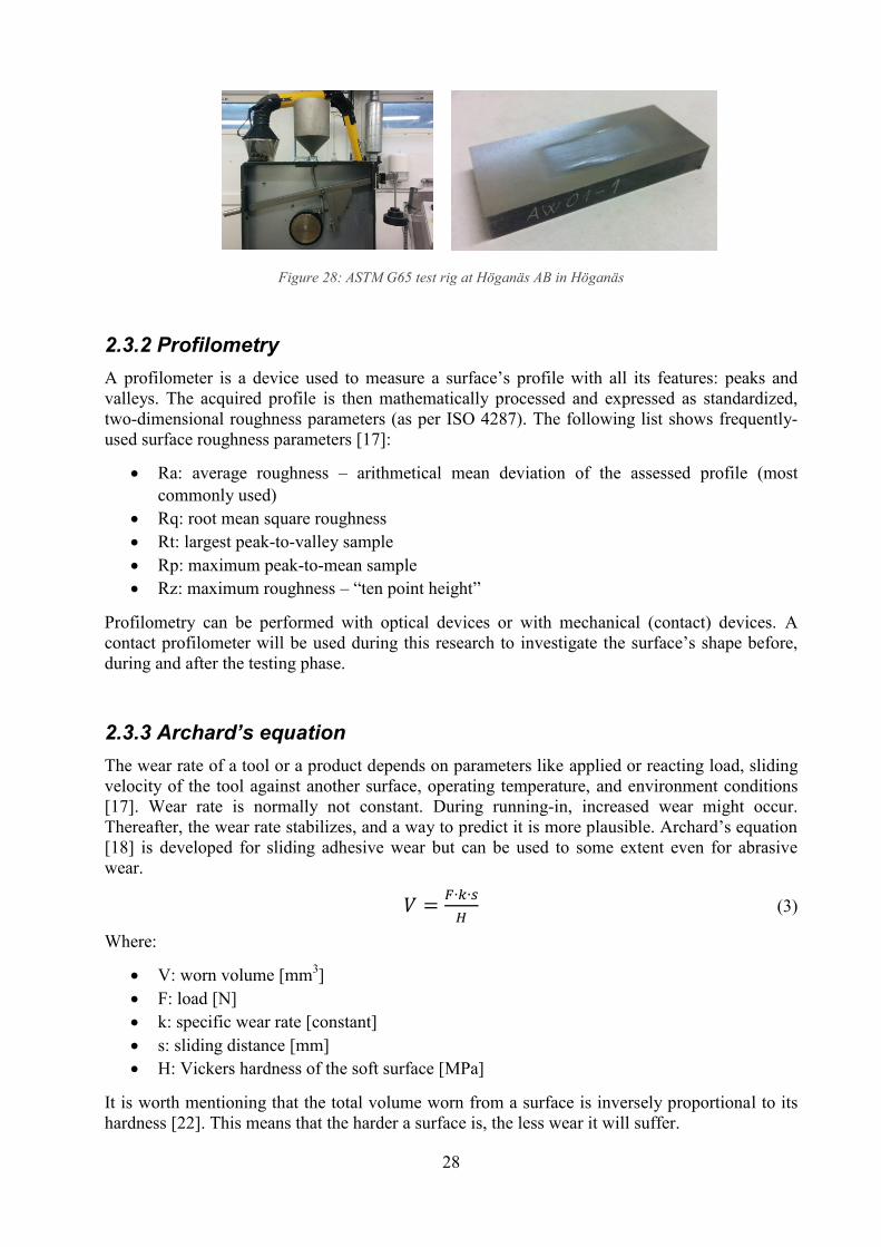
Figure 28: ASTM G65 test rig at Höganäs AB in Höganäs
2.3.2 Profilometry
A profilometer is a device used to measure a surface’s profile with all its features: peaks and
valleys. The acquired profile is then mathematically processed and expressed as standardized,
two-dimensional roughness parameters (as per ISO 4287). The following list shows frequently-
used surface roughness parameters [17]:
Ra: average roughness – arithmetical mean deviation of the assessed profile (most
commonly used)
Rq: root mean square roughness
Rt: largest peak-to-valley sample
Rp: maximum peak-to-mean sample
Rz: maximum roughness – “ten point height”
Profilometry can be performed with optical devices or with mechanical (contact) devices. A
contact profilometer will be used during this research to investigate the surface’s shape before,
during and after the testing phase.
2.3.3 Archard’s equation
The wear rate of a tool or a product depends on parameters like applied or reacting load, sliding
velocity of the tool against another surface, operating temperature, and environment conditions
[17]. Wear rate is normally not constant. During running-in, increased wear might occur.
Thereafter, the wear rate stabilizes, and a way to predict it is more plausible. Archard’s equation
[18] is developed for sliding adhesive wear but can be used to some extent even for abrasive
wear.
𝑉 =𝐹∙𝑘∙𝑠
𝐻 (3)
Where:
V: worn volume [mm3]
F: load [N]
k: specific wear rate [constant]
s: sliding distance [mm]
H: Vickers hardness of the soft surface [MPa]
It is worth mentioning that the total volume worn from a surface is inversely proportional to its
hardness [22]. This means that the harder a surface is, the less wear it will suffer.

29

30
2.4 Increasing resistance to abrasive wear
It is known that wear is a mechanical phenomenon that cannot be avoided, but the effects of
those mechanical interactions on tools can be minimized in several ways [17, 18]:
Increasing the hardness of the softest material until a difference between both materials is
less than 10% of the hardness.
Increasing the hardness of the material to at least 80% of the abrasive particles’ hardness.
Lower the roughness on the harder surface.
Coating the surface or embedding hard particles in the surface of the softer material (carbide-
forming metals when dealing with steels). Surface coatings can be applied by means of
several methods of which the relatively thick sprayed and overlay welded coatings are often
in use.
2.4.1 Laser cladding
Laser cladding is an advanced direct metal deposition process which creates a metallic
(metallurgical) bonding between the substrate and the cladding by means of intense heat, created
by a high-energy laser beam [26]. As explained before, the bonding of two dissimilar metals can
provide the substrate with a hard, stronger layer that endures abrasive and corrosive wear further.
Generally, the machinery required for this process to happen is composed of two main systems:
1. A powder feeder that delivers metallic powder to the substrate via a lateral nozzle and a
motion control system.
2. A laser generator attached to the three-dimensional positioning system (CAM-controlled) and
focusing optics which (vertically) direct the energy of the laser towards the substrate sample.
Figure 29: Laser cladding process [27]
The way the material is supplied onto the substrate can vary, since it can happen in a single-step
or in a two-step process [28]. The two-step technique requires that a powder be firstly pre-placed
onto the substrate, and then molten by the laser beam. This process takes longer time, but
requires a less complex delivery system. In the one-step technique, the coating material
(commonly powder metal) is delivered continuously into a laser-generated melt pool. That
means that both the laser and the delivery system’s nozzle move together.

31
The laser cladding process has several advantages [29]. It produces very low dilution of the
substrate material into the cladding, normally between 2% and 5% in a single layer. Compared to
a TIG/MIG overlay welding, the latter produces a dilution typically from 10% to 40%. In other
words, the target material composition can be achieved in a single layer, where a TIG/MIG
welding could require two or three layers. Wear and corrosion are effectively reduced by this
process, and that more complex, near-net-shape geometries can be coated [28]. Commercially,
applications of this process on near-net-shape pieces save considerable amounts of time and
resources, making the final product more competitive in the market.
This project deals with the plough point component mentioned in 1.1.1 GETs, where wear will
occur in the contact point with the ground at engagement, making laser cladding a great choice
of a process for coating the blade. Other advantages include low deformation of the substrate,
microstructure improvement through faster cooling rate, and the lack of cracks and porosity on
the product after finishing the process. Table 2 shows the materials which will be applied by
laser cladding on the substrate for testing of this project.
The increase in a tool’s resistance to abrasive wear (and thus total lifetime) will vary, depending
on the type of material which is deposited on the substrate. As mentioned, there is a wide range
of materials that can be deposited by means of laser cladding [28], which makes this process a
very versatile one. Höganäs’s equipment can reach a deposition rate of 8 kg/hour, a deposition
thickness of up to 4 mm, and a deposition hardness of 60+ HRC. This shows that laser cladding
can be a quick, automated process for wear protection of metals.

32

33
3. IMPLEMENTATION
This chapter explains which materials will be tested in the tribometer, under which conditions,
and the method to gather the information before and after the tests.
The work done during this project will be divided into two stages, consistently with the
objectives explained before in 1.2 Objectives and purpose. In total, three different material
configurations will be tested in the tribometer.
Table 5: Experimental setup
Material
designation Type Description Sand type
EN 22MnB5
Wrought
steel
reference
- Low alloyed through hardening steel with micro-
alloyed with B
W.-Nr.1.5531, Fe- 0.3 C- 1.25 Mn- 0.005 B
- 60 HRC
Silica
EN 22MnB5
Wrought
steel
reference
- Low alloyed through hardening steel with micro-
alloyed with B
W.-Nr.1.5531, Fe- 0.3 C- 1.25 Mn- 0.005 B
- 60 HRC
Kabelmjöl
Höganäs
1559-40
+50% 4590
Metal
powder +
carbide
powder mix
- Hard face: Ni-base with admixed relatively coarse
carbides
- Ni+<0.06 C- 3 Si- 2.9 B-0.2 Fe + 50% 4590 (WCx)
- 60+ HRC
Kabelmjöl
1. The reference steel (EN 22MnB5) will be run in silica sand, and then in Kabelmjöl sand. The
abrasive wear suffered on the same material under two different types of sand will be
compared. The wear caused on the blade by the reference material test will show which areas
shall be laser-cladded to run the following test. The carbide-overlaid material will only be
run in Kabelmjöl sand.
2. The worn blades will be transported to the Höganäs R&D laboratory for microscopic and
metallographic investigations.
3.1 Stage 1: performed at KTH
3.1.1 Carousel tribometer’s tool holder design
The tribometer designed by Anslin, Ferlin and Johansson [15] is located physically at KTH - The
Royal Institute of Technology, where the tribological tests will be performed. The machine
intends to simulate operating conditions of tractor ploughing, and its design parameters are
shown in Table 6. A very important component is the tool holder, which fixes the ploughshare in

34
the appropriate position, so that it’s dragged through the sand inside the drum to replicate actual
wear. The original holder is shown in Figure 30.
Figure 30: Original tool holder [15]
The tool holder, however, requires a more adequate design to simulate the real position and
depth of the ploughshare point during operation. The ploughshare point has a very particular
shape, which can be seen in Figure 31. The bending and the twisting angle must adapt to the tool
holder for the assembly to be closer to real-life mounting.
Figure 31: Kverneland ploughshare, complex bending
The actual tool positioning instruction, which was obtained by courtesy of Kverneland AS, is as
shown in Figure 32:
The long side of the ploughshare is set at a downward angle of 25° with respect to the
ground.
The short side of the ploughshare is tilted sideways by 15° with respect to the ground.
Figure 32: Actual ploughshare position (courtesy of Kverneland AS)

35
The data provided by Kverneland yielded the design shown in Figure 33, which holds the tool at
the precise depth of 20 cm below the surface of the sand, at the correct tilting and downward
angles with respect to the ground. The design requires three low-carbon steel parts to be welded
together, which should withstand the forces acting on the tool due to the weight of the granulate.
Figure 33: New tool holder design (left: frontal view, right: lateral view)
The new design was validated by means of an ANSYS simulation of the forces acting on the
surface of both the ploughshare and the holder. The input forces for simulation were taken from
the analysis performed by the team that built the tribometer [15], and a safety factor of 2 for
yield stress was used, which resulted in an applied force of 300 N on the tool. The simulation
yielded an approximate Von Mises equivalent stress of 170 MPa in the welded areas. To keep
the mass of the holder low, and to prevent elastic deformation of the thin plate on top of the
holder, the plate was reinforced with two welded ribs, as can be observed in the red circle on
Figure 33.
Figure 34: Stress simulation on new tool holder
Direction of movement

36
3.1.2 Setup and pre-processing of specimens
Correct positioning of the tool in the machine using the new tool holder is required for consistent
results. The tool is manually adjusted with screws until tight fastening is achieved, as in Figure
35.
Figure 35:Assembled tool inside tribometer
The amount of sand to be used during each test shall bury the tip of the ploughshare point under
20 cm of sand. Similar studies have used depths ranging from 15 to 30 cm to simulate tillage
operations [30, 31, 32]. This roughly translates into approximately 400 kg of sand, as per Figure
36. The pressure on the tool creates a drag force which the motor can easily overcome.
Figure 36: Sand mass calculations

37
3.1.3 Tribometer’s test parameters
As explained before, the motor installed on the tribometer has a fixed speed which allows
movement of the test blade through the sand. All the samples shall be run with the parameters
depicted on Table 6.
Table 6: Tribometer's operation parameters
Angular speed of the arm 63 RPM
Torque 552 Nm
Simulated tillage speed 10.13 km/hr
Run time for each day 22 hrs
Testing time for each day 2 hrs
Distance travelled each day 223 km
Daily runs are set to start approximately at 18:00 hrs. The tribometer then runs for 22 hrs without
interruption. The machine is to be stopped 22 hrs later (at 16:00 hrs on the next day), and some
minutes should be given for the dust to settle down inside the drum, to avoid contamination of
the surrounding environment by loose sand particles. Profilometry and weighing is performed
during 2 hours.
After measuring, the blade is fastened to the tool holder and then to the tribometer again. The lid
must always be fastened correctly to the tribometer, and masking tape or other types of sealing
should be placed in the gap between the lid and the drum to avoid any dust from escaping during
the test. This ensures a clean environment around the machine, and a consistent level of sand
throughout the test.
3.1.4 Method for surface profiling
Roughness measurements taken on the specimen’s surface, as explained in 2.3.2 Profilometry,
will allow to track how abrasive particles slowly wears the specimen. A high-precision
profilometer, model Taylor Hobson Form Talysurf, will be used for all measurements. A tool
holder was fabricated to firmly assemble the blade and to have a way to position the tool on the
profilometer’s table with certain precision, so all measurements are taken as close to each other
as possible. Five measurements along the Z axis, and six measurements along the X axis will be
taken from the working side of the blade, as shown in Table 7.
Method for measuring the surface roughness:
1. Remove all dust and rust particles from the blade’s surface by mild scrubbing with a brush
and cleaning with ethanol, then completely dry the blade.
2. Firmly screw the blade onto the blade holder, always in the same orientation.
3. Calibrate the stylus gage 1836 as per the machine’s calibration parameters.
4. Position the blade holder on the profilometer’s table as per Table 7.
5. Measure roughness profile and extract the graphs and results from the profilometer.

38
The selected amount of measurements and the displacement distance of the stylus aim at having
enough representative roughness data to track the development of the abrasive wear.
Table 7: Profilometry parameters
Figure 37: Taylor Hobson Form Talysurf surface profiler
3.1.5 Method for mass measurement
The mass of the blade will be measured daily, and its wear rate will be obtained from the
measurements. The instrument to be used is a precision scale, model Mettler Toledo XP2003S
with a precision of up to 0.001 grams.
Method for measuring mass:
1. Set the scale to zero grams.
2. Place the blade in a static position on the scale. The scale is to be set upside down for larger
area of contact with the plate, and it should be centered as much as possible for precision.
3. Repeat the measurement 3 times and obtain an average of the mass.

39
Figure 38:Mettler Toledo XP2003S equipment
3.2. Stage 2: performed at Höganäs AB
3.2.1 Method for cutting and sampling
Now that the ploughshare specimens have been weighed and their surface has been profiled,
small, observable samples from the tip of the ploughshare can be obtained by means of cutting,
grinding and polishing. The red square in Figure 39 shows the location of the sample. The idea is
that the microstructure and the carbides on the surface of the cladded sample can be observed.
Figure 39: Sample obtained from ploughshare specimens
The following method for obtaining the samples was performed following Höganäs’s norms:
1. One 5 x 10 mm sample will be cut by means of water jet from the side of the blade that was
exposed to wear. Cutting with water jet helps maintaining the sample cool, thus preserving its
microstructure. Additionally, the quality of water-jet cut is good enough to provide a sample
that must be only lightly grinded and polished without much effort.
2. The cutout is then placed in a thermoset resin fixture.
3. The sample is grinded with 80 and a 220-grain paper, cooled by water.
4. The sample is washed with ultrasonic vibrations between disk changes.
5. The sample is polished with 3 µm and a 1 µm polishing clothes with diamond abrasive, until
mirror finish is achieved.
6. The thermoset fixture is cracked open, and the sample is kept in a clean container for
analysis.

40
3.2.2 Method for electron microscope analysis
The scanning electron microscope (SEM) analysis will allow the observation of the
microstructure of the material to evaluate the size and distribution of the carbides from the laser
cladding process. The samples must be as clean and as free from electrostatic charge as possible,
and all security measures must be followed when using the microscope.
Method for analyzing the samples:
1. Each of the samples is to be cleaned with ethanol and a cotton to remove impurities and
grease from the surface.
2. The sample is then cleaned with acetone, and dried with hot air directly on the surface of the
sample.
3. All traces of cotton must be removed from the surface.
4. One sample at a time should be analyzed in the microscope.
5. The sample is placed on carbon tape onto a fixture, and the fixture is placed in the
microscope.
6. Intensity of electron beam, and visualization parameters can be set as needed.

41
4. RESULTS
This chapter presents the data gathered from the tribological tests performed in the custom made
tribometer.
4.1 Mass, wear rate and surface profile
The mass of each specimen was measured daily following the method explained in 3.1.5 Method
for mass. The data obtained from mass measurement yields the graphs from Figure 40 to Figure
42, which gives data for mass loss, wear rate and cumulative wear rate.
Table 8: Wear of the specimens - mass and volume loss summary
1 2 3 Ratio
3/2
Specimen material EN 22Mn B5 EN 22Mn B5 Höganäs
1559–40 + 50% 4590 -
Specimen material specific
density (g/cm3) 7.75 7.75 13 1.7
Abradant Silica Kabelmjöl Kabelmjöl -
Initial mass (g) 1317.095 1301.860 1334.691 -
Final mass (g) 1307.549 1279.820 1286.105 -
Total mass loss (g) 11.493 22.040 48.586 2.1
Mass loss from 1120 km (g) 3.643 1.842 0.556 0.30
Wear rate from 1120 km
(g/day) 0.924 0.273 0.077 0.28
Total volume loss (mm3) 1483 2844 3737 1.31
Volume loss from 1120 km
(mm3) 470 238 43 0.18
Wear rate from 1120 km
(mm3/day) 119 35 6 0.17
Mass loss is the subtraction of the final measured mass from the initially measured mass.
This subtraction may include the loss of paint and rust that may have already been found on
the tool’s surface before the tests had begun.
Mass loss from 1120 km is the subtraction of the final measured mass from the mass at 1120
km of travelled distance. This distance is the “stabilization point” after which the wear is
observed to behave linearly on all three samples.
Volume loss is obtained theoretically, dividing mass loss by specific density.
Wear rate is the average loss of mass per day starting from the stabilization point of 1120 km
of travelled distance.
The last column of Table 8 presents the ratio between the results of Tests 3 and 2 on each
row. It provides an easier way to interpret the results.

42
From Table 8, the following important observation can be noted. It is further addressed in 5.1
Discussion.
The laser-cladded sample, test 3, presents a specific density of approximately 13 g/cm3, since
carbides’ density must be accounted for, and not just the density of the EN 22MnB5 steel.
The 3/2 ratio of total mass loss is 2.1, and the ratio of total volume loss is 1.31.
The 3/2 ratio of total mass loss after the stabilization point is only 0.3. The volume loss ratio
is 0.18.
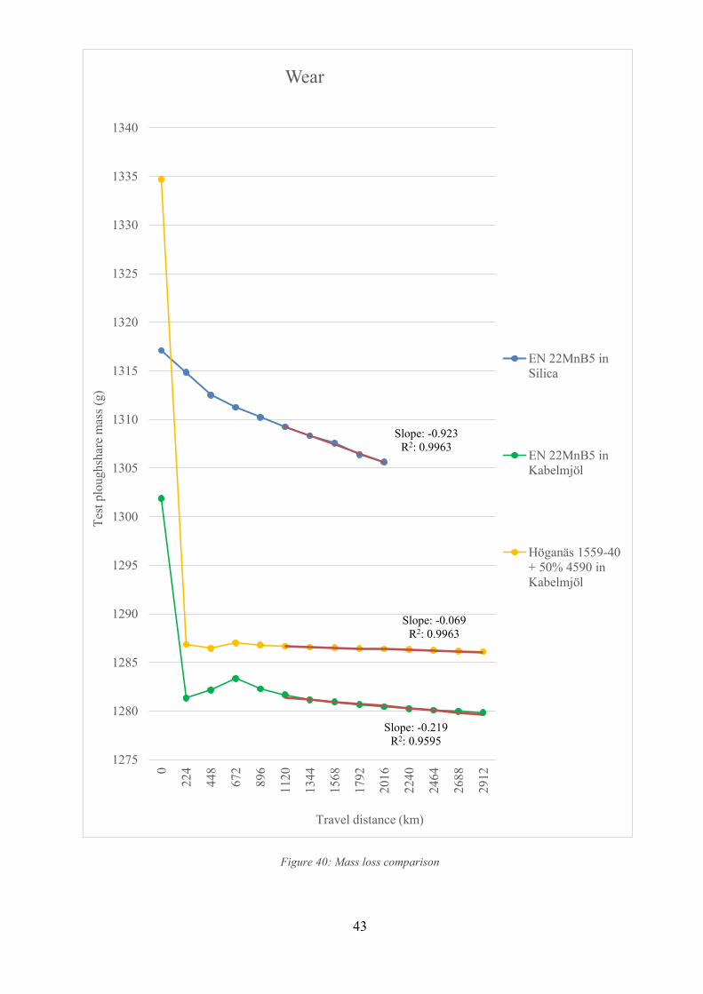
Figure 40 shows the mass of each specimen as travel distance increases. It is observed that a
gradual loss of mass is achieved on all specimens. However, only the specimen running in silica
sand (blue line) shows a continuously decreasing mass from beginning to end on all the days
when mass was measured. The other two specimens, which ran in Kabelmjöl sand, show a strong
loss of mass over the first 224 km. Thereafter, an increase in mass is evident from 224 km to 672
km of travelled distance. Finally, an almost linear mass loss is observed from 672 km.
It was observed that the loss of mass stabilizes on all three samples after 1120 km, since a linear
regression with R2 > 0.95 can be obtained.
The laser cladded sample is the one with the smallest loss of mass of all three samples after
stabilization, with a linear regression slope of -0.069 and a loss of only 0.556 g.
The largest loss of mass after stabilization was suffered by the EN 22MnB5 specimen running in
silica, with 3.643 g and a steeper slope of -0.923.
43
Figure 40: Mass loss comparison
1275
1280
1285
1290
1295
1300
1305
1310
1315
1320
1325
1330
1335
1340
0
22
4
44
8
672
89
6
11
20
13
44
15
68
17
92
20
16
22
40
24
64
26
88
29
12
Tes
t p
lou
gh
shar
e m
ass
(g)
Travel distance (km)
Wear
EN 22MnB5 in
Silica
EN 22MnB5 in
Kabelmjöl
Höganäs 1559-40
+ 50% 4590 in
Kabelmjöl
Slope: -0.923
R2: 0.9963
Slope: -0.219
R2: 0.9595
Slope: -0.069
R2: 0.9963

44
Figure 41: Wear rate comparison
-2,5
-2,0
-1,5
-1,0
-0,5
0,0
0,5
1,0
1,5
2,0
0
22
4
44
8
67
2
89
6
11
20
13
44
1568
17
92
20
16
22
40
24
64
26
88
29
12
Wea
r ra
te (
g/d
ay)
Travel distance (km)
Wear rate
EN 22MnB5 in
Silica
EN 22MnB5 in
Kabelmjöl
Höganäs 1559-40
+ 50% 4590 in
Kabelmjöl
Slope: 0.006
R2: 0.2387
Slope: 0.014
R2: 0.0196
Slope: 0.054
R2: 0.7649

45
Figure 42: Cumulative wear comparison
0
5
10
15
20
25
30
35
40
45
50
55
0
22
4
44
8
67
2
89
6
11
20
13
44
15
68
17
92
20
16
22
40
24
64
26
88
29
12
Cum
ula
tive
wea
r (g
)
Travel distance (km)
Cumulative wear
EN 22MnB5 in
Silica
EN 22MnB5 in
Kabelmjöl
Höganäs 1559-40 +
50% 4590 in
Kabelmjöl
Slope: 0.069
Slope: 0.923
Slope: 0.219

46
Figure 41 shows wear rate of the tested specimens. Given the large loss of mass during the first
448 km, the graph only shows the -2.5 to +2.5 g/day rate in the Y-axis scale, for ease-of-
visualization purposes. Because of division of numbers of similar size, the scatter is higher.
Additionally, the Kabelmjöl sand creates a coating on the surface of the tool which makes
measurements more inaccurate, since the samples cannot be cleaned easily.
4.1.1 Observations on EN 22MnB5 in silica sand
The silica sand provides a very abrasive environment. This can be supported by the relatively
steady mass loss observed in Figure 40. No mass gain was observed for this test.
Figure 43: Specimen EN 22MnB5 in silica (Day 0, 0 km travelled)
Figure 44: Specimen EN 22MnB5 in silica (Day 5, 1120 km travelled)
Figure 43 shows the initial state of the blade, which is covered with a thin layer of paint and
other imperfections. The point end of the blade is very sharp, and no chamfers or radii are
observed in any edge of the blade.
Figure 44 shows the blade after travelling 1120 km. A polished-like surface without as many
imperfections as during Day 0 was observed. On the frontal part of the blade, material ploughing

47
was observed, as well as abrasive wear tracks. The tip of the blade did not present significant
wear but some small rounding. By Day 5, most impurities from the surface had vanished, which
might correspond with the stabilization of the wear rate.
Figure 45: Specimen EN 22Mn5B in silica (Day 9, 2016 km travelled)
Figure 45 shows the final state of the blade, after travelling 2016 km. The surface appears to be
polish-finished, and the ploughing marks are clearly visible on the frontal surface of the blade.
The “dragged” or “ploughed” material observed on the frontal surface appears to be fractured or
worn-off.
Since a very linear behavior in the loss of mass was observed during this test after Day 3 (448
km) until Day 9 (2016 km), the test was stopped to assign more run time to the tests in
Kabelmjöl, since Kabelmjöl provides a more realistic simulation.

48
4.1.2 Observations on EN 22MnB5 in Kabelmjöl sand
Figure 46: Specimen EN 22MnB5 in Kabelmjöl (Day 0, 0 km travelled)
Figure 47: Specimen EN 22MnB5 in Kabelmjöl (Day 1, 224 km travelled)
Figure 46 (Day 0) shows a very rough finished surface on the original state of the specimen, and
a sharp tip of the blade can be observed. Thereafter, Figure 47 (Day 1, 224 km travelled) shows a
grinded surface with an opaque finish, and considerable wear is observed on the tip of the blade.

49
Figure 48: Specimen EN 22MnB5 in Kabelmjöl (Day 5, 1120 km travelled)
Figure 49: Specimen EN 22Mn5B in Kabelmjöl (Day 13, 2912 km travelled)
Figure 48 (Day 5, 1120 km) shows more surface imperfections on the blade as compared to Day
1. An adhered coating on the tool can be observed in brownish-color, like a mixture of oxides
and other ingredients. It is strongly adhered to the surface. Scrubbing it (as per 3.1.4 Method for
surface profiling) has no effect on it. However, the tip of the blade has not suffered much more
damage.

50
Figure 49 (Day 13, 2912 km) shows a whiter/browner surface, with little-to-no further damage
on the tip of the blade.
4.1.3 Observations on Höganäs 1559–40 + 50% 4590 in Kabelmjöl
sand
Figure 50: Specimen Höganäs 1559-40+50% 4590 in Kabelmjöl (Day 0, 0 km travelled)
Figure 51: Specimen Höganäs 1559-40+50% 4590 in Kabelmjöl (Day 1, 224 km travelled)

51
Figure 50 (Day 0, 0 km) shows the metal-powder coated sample, where the laser-cladded can be
clearly observed on the working end of the blade. Carbides provide a “shining”-like finish.
Figure 51 shows the specimen on Day 1 (224 km), where the base material suffers the same
“grinding” effect as the previous blade (Figure 47). The coated area doesn’t appear to have
suffered the “grinding” effect from the Kabelmjöl sand. However, the tip did suffer considerable
wear.
Figure 52: Specimen Höganäs 1559-40+50% 4590 in Kabelmjöl (Day 5, 1120 km travelled)
Figure 53: Specimen Höganäs 1559-40+50% 4590 in Kabelmjöl (Day 13, 2912 km travelled)

52
Figure 52 (Day 5, 1120 km) shows a more worn-out surface of the tool. The coating is holding,
and the “transition” between the base material and the coating is still quite evident. The same
brownish imperfections start to appear on the surface, as seen with EN 22MnB5 in Kabelmjöl
sand. The tip of the tool suffered no further damage, compared to Day 1.
Figure 53 (Day 13, 2912 km) presents the final state of the blade after testing. The “transition”
between the base material (marked with a red arrow) and the coating are a bit smoother, as if the
coating degraded a little. Figure 59 presents the surface profile for this phenomenon.

53
4.2 Surface roughness
By following the method described in 3.1.4 Method for surface profiling, the roughness data for
the surface of each specimen, as well as its surface profile plot were obtained. The following
charts present only the Ra and Rz parameters for ease of understanding. The surface profile plots
are presented to observe how the surface of each sample is affected by wear. Although many
profiles were obtained daily following the method in 3.1.4 Method for surface profiling, this
chapter presents horizontal and vertical lines close to the area where the physical samples were
cut-out with water jet.
Complete roughness graphs for horizontal and vertical measurements can be found in
APPENDIX C: SURFACE ROUGHNESS – FULL CHARTS.
Figure 54: Average surface roughness - EN 22MnB5 in silica
Figure 54 shows a steady decrease in roughness from Day 0 to Day 3 (672 km), when the sand
begins to roughen the surface of the blade. Day 6 (1344 km) shows a strong spike in overall
roughness. Thereafter, roughness decreases again until Day 8 (1792 km), and it finally increases
again in Day 9 (2016 km). The behavior is erratic.
0,02
0,03
0,06
0,13
0,25
0,50
1,00
2,00
4,00
0
448
672
896
1120
1344
1568
1792
2016
Roughnes
s (µ
m)
Travelled distance (km)
Average roughness
EN 22MnB5 in silica sand
Ra
Rz
54
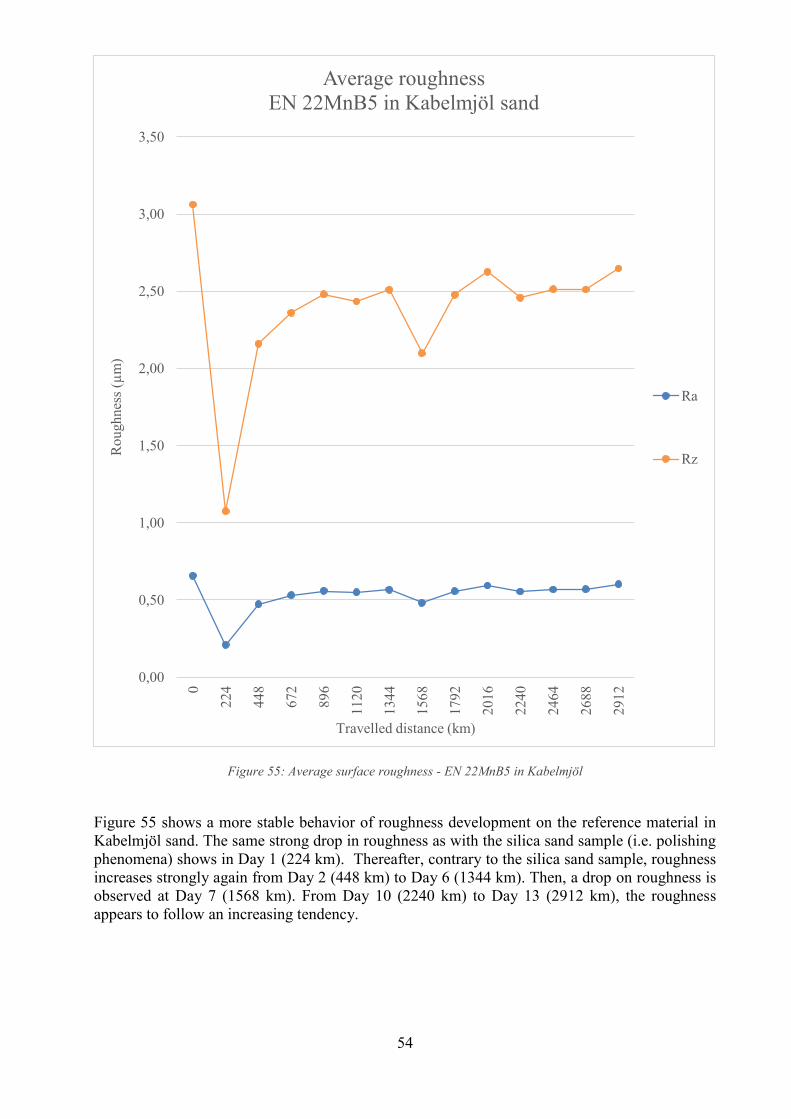
Figure 55: Average surface roughness - EN 22MnB5 in Kabelmjöl
Figure 55 shows a more stable behavior of roughness development on the reference material in
Kabelmjöl sand. The same strong drop in roughness as with the silica sand sample (i.e. polishing
phenomena) shows in Day 1 (224 km). Thereafter, contrary to the silica sand sample, roughness
increases strongly again from Day 2 (448 km) to Day 6 (1344 km). Then, a drop on roughness is
observed at Day 7 (1568 km). From Day 10 (2240 km) to Day 13 (2912 km), the roughness
appears to follow an increasing tendency.
0,00
0,50
1,00
1,50
2,00
2,50
3,00
3,50
0
224
448
672
896
1120
1344
1568
1792
2016
2240
2464
2688
2912
Rou
gh
nes
s (µ
m)
Travelled distance (km)
Average roughness
EN 22MnB5 in Kabelmjöl sand
Ra
Rz

55
Figure 56: Average surface roughness - Höganäs 1559-40+50% 4590 in Kabelmjöl
Figure 56 shows the roughness development on the laser cladded sample, which follows a very
similar pattern compared to the reference material in Kabelmjöl sand (Figure 55). The same
strong roughness drop in Day 1, the same increase from Day 2 to Day 6, and the same sudden
drop in roughness on Day 7 are observed. However, roughness drops continuously from Day 8
(1792 km), which appears to follow a linear tendency.
0,25
0,50
1,00
2,00
4,00
8,00
0
224
448
672
896
1120
1344
1568
1792
2016
2240
2464
2912
Rou
gh
nes
s (µ
m)
Travelled distance (km)
Average roughness
Höganäs 1559-40+50% 4590 in Kabelmjöl sand
Ra
Rz

56
4.2.1 Surface profile – EN 22MnB5 in silica sand
Figure 57: Surface profile, EN 22MnB5 in silica sand
Figure 57 shows a sketch of the surface profile evolution during the test on silica sand, which
gives an idea of how the surface is affected by the sand. The green line shows Day 0 (original
surface), which is rather rough. The red line shows the measurement on Day 2, the black line
shows Day 5, and the blue line shows Day 9.
Day 0 presents a rougher surface than other days’ profiles. As the test advances, this specimen
showed a continuously smoother surface, reaching a mirror-like polished finish at Day 9. Figure
58 shows how the share point looks like after 9 days of wear, which corresponds to the flatter
blue line in Figure 57.
Figure 58: EN 22MnB5 sample after 9 days of testing in silica sand

57
4.2.2 Surface profile – EN 22MnB5 in Kabelmjöl sand
Figure 59: Surface profile, EN 22MnB5 in Kabelmjöl sand
Figure 59 shows a sketch of the surface profile evolution during the test of the EN 22MnB5 test
in Kabelmjöl sand. The green line shows Day 0 (original surface). The red line shows the
measurement on Day 1, the blue line shows Day 5, and the black line shows Day 13.
Day 1 presents a smoother surface than Day 0, which confirms what can be observed on the
specimen: a grinded-like finish of the surface. Day 5 shows a further deformed surface opposite
to the tip of the share point (see Figure 60). Day 13 presents a smoother surface, yet somewhat
deformed away from the tip. The tip kept a rather smooth surface throughout the entire test.
Figure 60: EN 22MnB5 sample after 5 days of testing in Kabelmjöl sand

58
4.2.3 Surface profile – Höganäs 1559-40+50% 4590 in Kabelmjöl sand
Figure 61: Surface profile, Höganäs 1559-40+50% 4590 in Kabelmjöl sand
Figure 61 shows a sketch of the surface profile evolution during the test of the 1559-40+50%
4590 material in Kabelmjöl sand. The green line shows Day 0 (original surface). The red line
shows the measurement on Day 1, the blue line shows Day 5, and the black line shows Day 13.
A steep step (transition from base material to coating) from Day 0 can be observed, as the laser
cladding is new and well-defined. At Day 1, the step has smoothened, and a small radius
develops as time passes, as if the transition began to disappear gradually. Some deformation can
be observed in Day 5 close to the coated area, but still on the base material. On Day 13, the
surface appears smoother, and the step decreased slightly.
All original profiles are available as APPENDIX D: SURFACE PROFILE – INDIVIDUAL
GRAPHS.

59
4.3 Cut samples
Figure 62: Extracted samples (top: EN 22MnB5 in silica, middle: EN 22MnB5 in Kabelmjöl,
bottom: carbide coated EN 22MnB5)
Figure 63: Carbide coated blade, frontal view

60
Figure 64: Carbide coated blade, side view
Figure 62 shows the water-jet-cut specimens for later analysis of the sample under the
microscope. Figure 63 and Figure 64 show the Höganäs 1559-40+50% 4590 specimen’s carbide
coating in darker gray shades. As mentioned before, the quality of the water jet cut is good
enough to provide a sample that must be lightly grinded and polished without much effort, while
keeping the sample cool enough to not alter its microstructure. The reddish marks in the cut area
of Figure 64 are corrosion after water jet cutting.

61
4.4 Microscopy
A scanning electron microscope (FEG SEM Hitachi SU6600) analysis was performed on the
samples taken from the specimens shown in Figure 62, and the results are presented in Figure 65
to Figure 67.
Figure 65: EN 22MnB5 worn in silica sand
Figure 65 shows several microscopies for the silica sand test. Sand flow is indicated on top to
understand how the sand abrades the specimen. The base matrix of the specimen can be seen in
light gray color, and some sand can be observed as white spots on the top pictures.

62
Figure 66: EN 22MnB5 worn in Kabelmjöl sand
Figure 66 shows the EN 22MnB5 specimen’s microscopy in Kabelmjöl sand, where a little more
sand can be observed as white spots in the gray matrix of the sample. The wear is difficult to
perceive on the surface. The sand flow is also shown as orange arrows.

63
Figure 67: Höganäs 1559-40+50% 4590 worn in Kabelmjöl sand
In Figure 67 , the circular carbides of the Höganäs 1559-40+50% 4590 specimen in Kabelmjöl
sand are visible in bright white color on the cladded area. The carbides are evenly but coarsely
dispersed, evenly in the matrix.

64
4.5 Sand analysis
The Ottawa silica sand and the Kabelmjöl sand were analysed after finishing the tests. Table 9
lists particle morphology parameters analysed on as run sand in test run. These results are to
illustrate how the particle morphology looks like, while a detailed investigation demands
extended resources and is left for future work. Briefly, the Kabelmjöl sand, in comparison to the
silica sand, has a higher aspect ratio, a lower sphericity and almost equal perimeter ratio.
Table 9: Particle shape analysis by Leica QWin software at Höganäs AB
Sand Aspect Ratio Sphericity Perimeter Ratio
Silica 1.477 0.629 0.831
Kabelmjöl 1.734 0.467 0.790
In addition, XRD analysis of the sand was performed by courtesy of Dr. Björn Skårman,
Höganäs AB. The results are presented from Figure 68 to Figure 70. The sand samples were
taken from an area above the tip of the ploughshare point when it is mounted in the tribometer.
Figure 68: XRD Crystallinity analysis of the sand (above and below the tip)
Figure 68 shows that the sand above the tip of the blade includes more crystalline components.
Figure 69: Chemical composition - sand below tip of the blade
Figure 69 shows the chemical analysis of the sand below the tip of the blade. Quartz (SiO2) and
Albite (AlNaSi3O8) with Mohs hardness of 6 to 6.5 were found.
Arbitrary intensity
(counts)
Arbitrary intensity
(counts)
2 (degrees)
2 (degrees)

65
Figure 70: Chemical composition - sand above tip of the blade
Figure 70 shows the chemical analysis of the sand above the tip of the blade. Quartz (SiO2),
Albite (AlNaSi3O8) and Analcime 1O (H2AlNaSi2O7) with Mohs hardness of 5 to 5.5 were
found.
Deeper hardness analysis of the test sands also demands extended resources and is left for future
work.
4.6 Other observations
The tribometer’s wall (the drum) experiences visible swinging during the first 22 hrs of
testing with new sand.
At some point, the thicker sand has moved to the bottom of the drum, and the finer sand
remains on top. This was consistent with both silica sand and Kabelmjöl sand.
Another explanation for the drop on wear rate as time increases would be the work-hardening
of the blade as travel distance increases. Hardel et al [24] have found that boron steels can
increase wear resistance due to work hardening. This would be consistent with the sand
degrading rapidly and the resistance of the blade increasing at the same time, which in
combination, would cause a much lower wear rate after some hours.
Arbitrary intensity
(counts)
2 (degrees)

66

67
5. DISCUSSION AND CONCLUSIONS
This chapter discusses the findings from the results section in order to explain the phenomena
that was observed.
5.1 Discussion
Stage 1:
Will the abrasive wear resistance ranking be the same between the carousel tribometer
and the ASTM G65 testing?
o The Höganäs 1559-40+50% 4590 sample presented the smallest loss of mass after the
stabilization point of Day 5, with 0.55 g lost in 1792km. This represents a 30% of the
wear on EN 22MnB5. However, the volume loss is only 18% of the wear on the
reference sample (see Table 8). Carbides are much denser than steel, and therefore,
the specific density of the laser-cladded and the reference samples differs.
o Volumetric loss should be used to calculate wear, instead of mass loss, due to the
explanation above.
o Wear rate decreases strongly after the first day of tests in all materials. The tips of all
three blades suffer severe wear during the first day of tests as well. An explanation for
the drop on wear rate as time increases would be the work-hardening of the blade as
travel distance increases. Hardel et al [24] found that boron steels can increase wear
resistance due to work hardening.
o As with mass loss, the wear rate is considerably lower when using volumetric loss
rate to calculate it (only 17% of the reference material’s wear rate).
o Thus, the carousel tribometer abides to the results of the ASTM G65 test, which
means the ranking can be considered to be the same.
Will the hard phase particle size be the strongest factor again, compared to the previous
study [13]?
o Only one specimen contained carbides during these tests, so it cannot be compared to
previous results in terms of particle sizes.
o However, the sample with carbides was the one that presented the lowest wear of all
three specimens.
o The number of laser cladded variants of the tool was reduced to only one, because of
other activities in the room where the tribometer was placed
Stage 2:
How does the wear pattern look like?
o The wear pattern looks very similar in all three specimen samples. The sand flow is
the same for all samples, and the same areas are worn out on all samples (mainly the
tip of the blade).

68
o Kabelmjöl sand creates a coating on the sample’s surface that is difficult to remove,
which affects the accuracy of the roughness measurements. The samples can be
thoroughly cleaned to minimize this effect, but this question is best to be left for
future work.
How does the wear pattern develop with time?
o A rough surface from Day 0 becomes smooth (as grinded or polished) after the first
one or two days. This was visible on all three specimens.
o Thereafter, an increase in roughness was noted for the samples in Kabelmjöl sand, but
the sample in silica sand kept smoothening throughout the test.
o The roundish silica grains’ geometry might be accountable for this, in comparison
with the angularish geometry of Kabelmjöl.
How do the hard phase and matrix wear look like, and what is the hard phase particle
size?
o The round carbides are distributed quite evenly in the matrix, but the carbide fraction
density could be higher.
o Figure 67 shows some irregular clusters of carbides closer to the “C” side of the
sample. Laser cladding parameters need adjustment to create a more even distribution
of carbides, and a higher percentage of the carbides in the matrix.
Is there a possibility to improve the ploughshare design?
o From these tests, a more appropriate design cannot be proposed. Another longer test
run is needed in combination with a more abrasive test sand.
What sections of the ploughshare’s surface should be hard faced?
o Significant wear was not evident by coating the frontal edge of the blade. This has
proven to be enough for this testing duration.
5.2 Conclusions
Abrasive wear testing was conducted on three ploughshare specimens in a custom designed
tribometer for Höganäs AB. The sample materials were EN 22MnB5 steel and Höganäs 1559-
40+50% 4590 laser-cladded hard overlay, and the abrasive sands used were silica sand and
Kabelmjöl (granite) sand.
The laser-cladded sample resulted in 18% lower volume loss or 5.6 times lower wear in
comparison with EN 22MnB5 steel without carbide coating. The wear should be reported as
volume loss due to the difference in specific densities of the steel sample and the carbide-coated
sample.
This follows the same ranking of the results given by the ASTM G65 test, and proves that the
carousel tribometer can be used for simulating abrasive wear in ploughshare point tools.
An overlay welding area for the tool was proposed and tested, and the microstructure showed
quite even dispersion of round carbides with few irregular distribution clusters. The
microstructure can be improved further by adjusting cladding parameters.

69
6. FUTURE WORK
This chapter discusses what further steps can be taken to further analyze the behavior of the
material.
6.1 Future work
For future research, the following points are of interest:
A continuous increase in wear decrease of mass during the silica sand test, compared to the
Kabelmjöl sand test, where sudden increases of mass are evident.
The polishing of the ploughshare sample when running in silica sand.
The adhered layer appearing on the surface of the Kabelmjöl sand tests, its composition and
effect on wear.
Temperature inside the drum due to friction between the sand and the tool, and its effect on
the wear.
Humidity in the sand, and its effect on the wear.
The hardness analysis of the test sands.

70

71
7. REFERENCES
[1] A. P. Dedousis and T. Bartzanas, Soil Engineering, Heidelberg: Springer, 2010.
[2] The Grains Research and Development Corporation, "GCTV12: Mouldboard Ploughing -
Pros & Cons," 2013. [Online]. Available: https://youtu.be/Xf52ZemlY20.
[3] Ellis Machinery, "Kverneland EO85/300 7F Plough (9139)," 2017. [Online]. Available:
http://www.ellismachinery.co.uk/product/kverneland-eo85-300-7f-plough-9139.
[4] T. Eyre, "Wear characteristics of metals," Tribology International 9, pp. 203-212, 1976.
[5] P. S. Mann and N. K. Brar, "Tribological aspects of agricultural equipments: a review,"
International Research Journal of Engineering and Technology, pp. Volume 02, Issue 03,
2015.
[6] A. Natsis, G. Petropoulos and C. Pandazaras, "Influence of local soil conditions on
mouldboard ploughshare abrasive wear," Tribology International 41, pp. 151-157, 2008.
[7] V. Sastri, Challenges in corrosion: costs, causes, consequences, and control, New Jersey:
Wiley, 2015.
[8] Y. Bayhan, "Reduction of wear via hardfacing of chisel ploughshare," Tribology
International 39, pp. 570-574, 2006.
[9] Lindéngruppen AB, "Höganäs AB," 2017. [Online]. Available:
http://www.lindengruppen.com/hoganas-ab/hoganas-ab.
[10] Höganäs AB, "Surface coating," 2017. [Online]. Available:
http://www.hoganasthermalspray.com.
[11] ASTM International, G65: Standard test method for measuring abrasion using the dry
sand/rubber wheel apparatus, ASTM International, 2016.
[12] T. Mang and W. Dresel, Lubricants and Lubrication, 2 Volume Set, Wiley, 2017.
[13] S. Dizdar and B. Maroli, "Abrasive wear resistance of thermal surfacing materials," in
International Thermal Spray Conference and Exposition, Busan, South Korea, 2013.
[14] S. Dizdar, Abrasive wear testing levels, Höganäs AB, 2017.
[15] M. Anslin, J. Ferlin and V. Johansson, Development of an abrasive wear tribometer,
Stockholm: KTH Royal Institute of Technology, 2016.
[16] N. R. AB, "NCC Arlanda Kabelmjöl specification," 2013.
[17] A. van Beek, Advanced engineering design: Lifetime performance and reliability, TU Delft,
2009.
[18] G. W. Stachowiak and A. W. Batchelor, Engineering tribology, Butterworth-Heinemann,
2013.
[19] F. Campbell, Elements of metallurgy and engineering alloy, ASTM International, 2008.
[20] R. E. White, Principles and practice of soil science, Blackwell Publishing, 2006.
[21] B. Bhushan, Introduction to tribology, Columbus: Wiley, 2013.

72
[22] A. Zmitrowicz, "Wear patterns and laws of wear - a review," Journal of Theoretical and
Applied Mechanics 44, pp. 219-253, 2006.
[23] ASTM International, G76: Standard Test Method for Conducting Erosion Tests by Solid
Particle Impingement Using Gas Jets, ASTM International, 2017.
[24] J. Hardell, A. Yousfi, M. Lund, L. Pelcastre and B. Prakash, "Abrasive wear behaviour of
hardened high strength boron steel," Tribology, vol. 8 No 2, 2014.
[25] G. Stachowiak, G. Stachowiak, D. De Pellegrin and P. Podsiadlo, Wear - materials,
mechanisms and practice, John Wiley & Sons, 2014.
[26] Höganäs AB, "Laser cladding," 2016. [Online]. Available:
https://www.hoganas.com/en/business-areas/surface-coating/products/deposition-
techniques/laser-cladding/.
[27] Metal Additive Manufacturing, "Metal additive manufacturing processes," 2017. [Online].
Available: http://www.metal-am.com/introduction-to-metal-additive-manufacturing-and-3d-
printing/metal-additive-manufacturing-processes/.
[28] R. Vilar, "Laser cladding," Journal of laser applications, pp. 64-79, 1999.
[29] L. F. Pease and W. G. West, Fundamentals of powder metallurgy, Princeton: Metal Powder
Industries Federation, 2002.
[30] A. Hemmat, I. Ahmadi and A. Masoumi, "Water infiltration and clod size distribution as
influenced by ploughshare type, soil water content and ploughing depth," Biosystems
Engineering 97, pp. 257-266, 2007.
[31] E. Y. Bobobee and G. Gebresenbet, "Effect of cutting edge thickness and state of wear of
ploughshare on draught force and heart rates of Sanga oxen in Ghana," Soil & Tillage
Research 95, pp. 298-307, 2007.
[32] A. Yazici, "Wear behavior of carbonitride-treated ploughshares produced from 30MnB5
steel for soil tillage applications," Metal Science and Heat Treatment 53, 2011.
[33] I. Kovaříková, B. Szewczyková, P. Blaškoviš, E. Hodúlová and E. Lechovič, "Study and
characteristic of abrasive wear mechanisms," Slovak Research and Development Agency,
Trnava, 2009.
[34] J. Fernández, R. Vijande, R. Tucho, J. Rodríguez and A. Martín, "Materials selection to
excavator teeth in mining industry," Wear 250, pp. 11-18, 2001.
[35] M. Alamouti and M. Navabzadeh, "Investigation of plowing depth effect on some soil
physical properties," Pakistan Journal of Biological Sciences, pp. 10(24):4510-4, 2007.
[36] S. Nowotny, L.-M. Berger and J. Spatzier, "Coatings by laser cladding," Comprehensive
hard materials, pp. 507-525, 2014.
[37] Food and Agriculture Organization of the United Nations, "Better Farming Series 07 Crop
Farming," 1976. [Online]. Available: http://www.nzdl.org/gsdlmod?e=d-00000-00---off-
0unescoen--00-0----0-10-0---0---0direct-10---4-------0-1l--11-en-50---20-about---00-0-1-00-
0--4----0-0-11-10-0utfZz-8-
00&a=d&c=unescoen&cl=CL1.1&d=HASH1eedb5a59b9526c7cdbaac.2.3.
[38] Gesellschaft für Tribologie e.V., "Arbeitsblatt 7 – Tribologie Definitionen, Begriffe,
Prüfung," 2002. [Online]. Available: http://gft-ev.de/wp-

73
content/uploads/2014/07/2002_AB_7_Tribologie.pdf.
[39] Wikimedia Foundation Inc, "Granite Chemical composition," June 2017. [Online].
Available: https://en.wikipedia.org/wiki/Granite#Chemical_composition. [Accessed June
2017].

74

75
LIST OF FIGURES
Figure 1: Kverneland reversible ploughshare point, model 063090 (courtesy of Kverneland AS) 9
Figure 2: Plough assembly [3]....................................................................................................... 10
Figure 3: Tribological tests categories [12] ................................................................................... 12
Figure 4: Plough abrasive wear testing categorization based on DIN 5032 [14] .......................... 13
Figure 5: Carousel tribometer [15] ................................................................................................ 13
Figure 6: The process of wear ....................................................................................................... 17
Figure 7: Development of fatigue wear [18] ................................................................................. 18
Figure 8: Flake caused by fatigue wear [18] ................................................................................. 18
Figure 9: Process of corrosion wear [18] ...................................................................................... 19
Figure 10: Evidence of corrosive wear [17] .................................................................................. 20
Figure 11: Material transfer between asperities [17] ..................................................................... 20
Figure 12: Development of adhesive wear [18] ............................................................................ 20
Figure 13: Modes of abrasive wear [17] ....................................................................................... 21
Figure 14: Abrasive wear model [4] .............................................................................................. 21
Figure 15: Two and three-body abrasive systems [18] ................................................................. 22
Figure 16: Abrasion failure modes [18] ........................................................................................ 22
Figure 17: Scratched surface due to abrasion [21] ........................................................................ 23
Figure 18: Ploughing and cutting due to abrasion [21] ................................................................. 23
Figure 19: Erosive wear [21] ......................................................................................................... 23
Figure 20: Relative wear resistance vs hardness ratio [18] ........................................................... 24
Figure 21: Particle diameter vs wear rate [18] .............................................................................. 25
Figure 22: Particle size vs wear rate in two-body abrasion [25] ................................................... 25
Figure 23: Particle shape [25] ....................................................................................................... 25
Figure 24: Particle shape, SP approach [18] ................................................................................. 26
Figure 25: Particle shape, SPQ approach [18] .............................................................................. 26
Figure 26: Brittleness of particles [18] .......................................................................................... 27
Figure 27: ASTM G65 schematic [11] .......................................................................................... 27
Figure 28: ASTM G65 test rig at Höganäs AB in Höganäs .......................................................... 28
Figure 29: Laser cladding process [27] ......................................................................................... 30
Figure 30: Original tool holder [15] .............................................................................................. 34
Figure 31: Kverneland ploughshare, complex bending ................................................................. 34
Figure 32: Actual ploughshare position (courtesy of Kverneland AS) ......................................... 34

76
Figure 33: New tool holder design (left: frontal view, right: lateral view) ................................... 35
Figure 34: Stress simulation on new tool holder ........................................................................... 35
Figure 35:Assembled tool inside tribometer ................................................................................. 36
Figure 36: Sand mass calculations ................................................................................................ 36
Figure 37: Taylor Hobson Form Talysurf surface profiler ............................................................ 38
Figure 38:Mettler Toledo XP2003S equipment ............................................................................ 39
Figure 39: Sample obtained from ploughshare specimens ............................................................ 39
Figure 40: Mass loss comparison .................................................................................................. 43
Figure 41: Wear rate comparison .................................................................................................. 44
Figure 42: Cumulative wear comparison ...................................................................................... 45
Figure 43: Specimen EN 22MnB5 in silica (Day 0, 0 km travelled) ............................................ 46
Figure 44: Specimen EN 22MnB5 in silica (Day 5, 1120 km travelled) ...................................... 46
Figure 45: Specimen EN 22Mn5B in silica (Day 9, 2016 km travelled) ...................................... 47
Figure 46: Specimen EN 22MnB5 in Kabelmjöl (Day 0, 0 km travelled) .................................... 48
Figure 47: Specimen EN 22MnB5 in Kabelmjöl (Day 1, 224 km travelled) ................................ 48
Figure 48: Specimen EN 22MnB5 in Kabelmjöl (Day 5, 1120 km travelled) .............................. 49
Figure 49: Specimen EN 22Mn5B in Kabelmjöl (Day 13, 2912 km travelled) ............................ 49
Figure 50: Specimen Höganäs 1559-40+50% 4590 in Kabelmjöl (Day 0, 0 km travelled) ......... 50
Figure 51: Specimen Höganäs 1559-40+50% 4590 in Kabelmjöl (Day 1, 224 km travelled) ..... 50
Figure 52: Specimen Höganäs 1559-40+50% 4590 in Kabelmjöl (Day 5, 1120 km travelled) ... 51
Figure 53: Specimen Höganäs 1559-40+50% 4590 in Kabelmjöl (Day 13, 2912 km travelled) . 51
Figure 54: Average surface roughness - EN 22MnB5 in silica ..................................................... 53
Figure 55: Average surface roughness - EN 22MnB5 in Kabelmjöl ............................................ 54
Figure 56: Average surface roughness - Höganäs 1559-40+50% 4590 in Kabelmjöl .................. 55
Figure 57: Surface profile, EN 22MnB5 in silica sand ................................................................. 56
Figure 58: EN 22MnB5 sample after 9 days of testing in silica sand ........................................... 56
Figure 59: Surface profile, EN 22MnB5 in Kabelmjöl sand ......................................................... 57
Figure 60: EN 22MnB5 sample after 5 days of testing in Kabelmjöl sand ................................... 57
Figure 61: Surface profile, Höganäs 1559-40+50% 4590 in Kabelmjöl sand .............................. 58
Figure 62: Extracted samples (top: EN 22MnB5 in silica, middle: EN 22MnB5 in Kabelmjöl,
bottom: carbide coated EN 22MnB5) ........................................................................................... 59
Figure 63: Carbide coated blade, frontal view .............................................................................. 59
Figure 64: Carbide coated blade, side view .................................................................................. 60
Figure 65: EN 22MnB5 worn in silica sand .................................................................................. 61
Figure 66: EN 22MnB5 worn in Kabelmjöl sand ......................................................................... 62
Figure 67: Höganäs 1559-40+50% 4590 worn in Kabelmjöl sand ............................................... 63
Figure 68: XRD Crystallinity analysis of the sand (above and below the tip) .............................. 64

77
Figure 69: Chemical composition - sand below tip of the blade ................................................... 64
Figure 70: Chemical composition - sand above tip of the blade ................................................... 65

78

79
LIST OF TABLES
Table 1: Mohs scale of hardness ................................................................................................... 10
Table 2: Materials to be tested ...................................................................................................... 14
Table 3: Silica sand properties ...................................................................................................... 14
Table 4: Kabelmjöl sand properties [16] ....................................................................................... 14
Table 5: Experimental setup .......................................................................................................... 33
Table 6: Tribometer's operation parameters .................................................................................. 37
Table 7: Profilometry parameters .................................................................................................. 38
Table 8: Wear of the specimens - mass and volume loss summary .............................................. 41
Table 9: Particle shape analysis by Leica QWin software at Höganäs AB ................................... 64

80
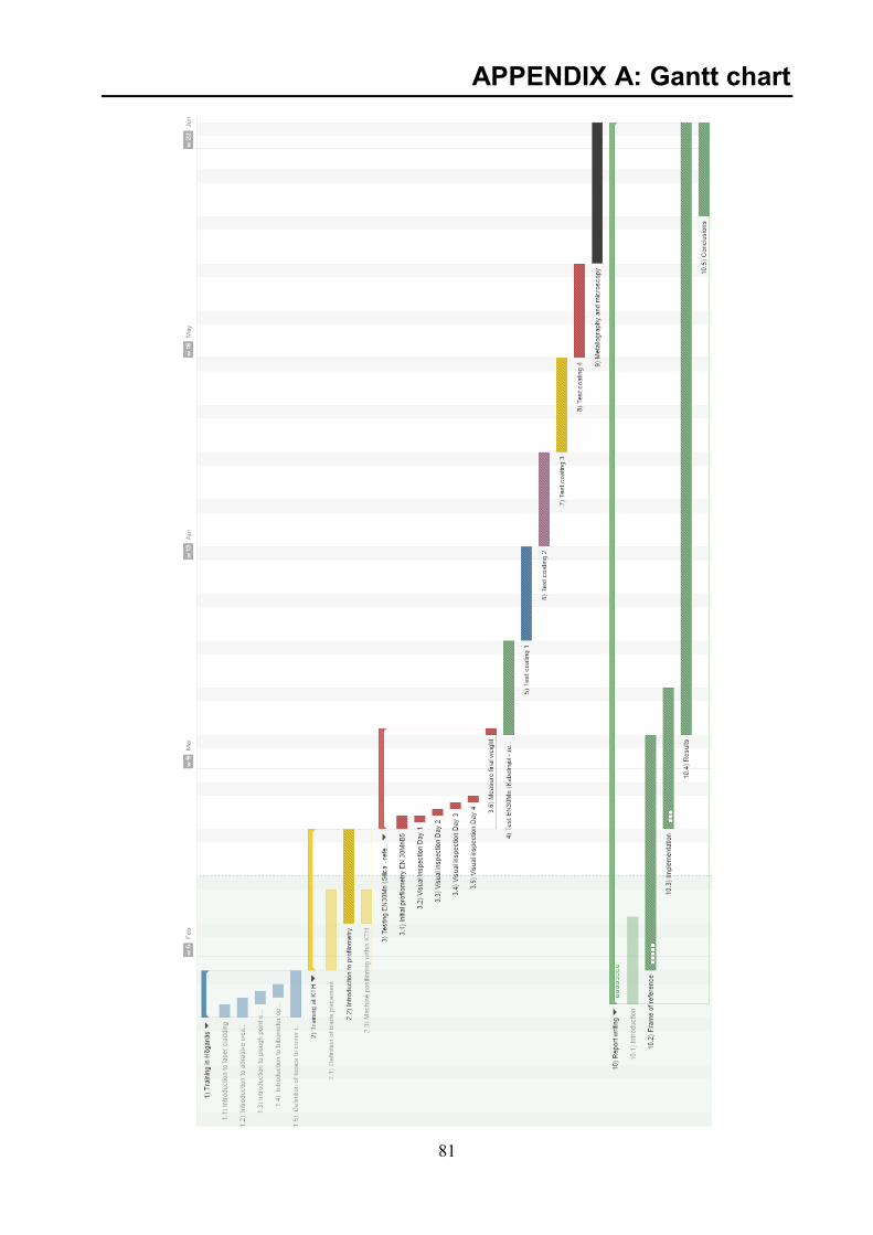
81
APPENDIX A: Gantt chart

82
APPENDIX B: NCC Arlanda Kabelmjöl specification

83

84
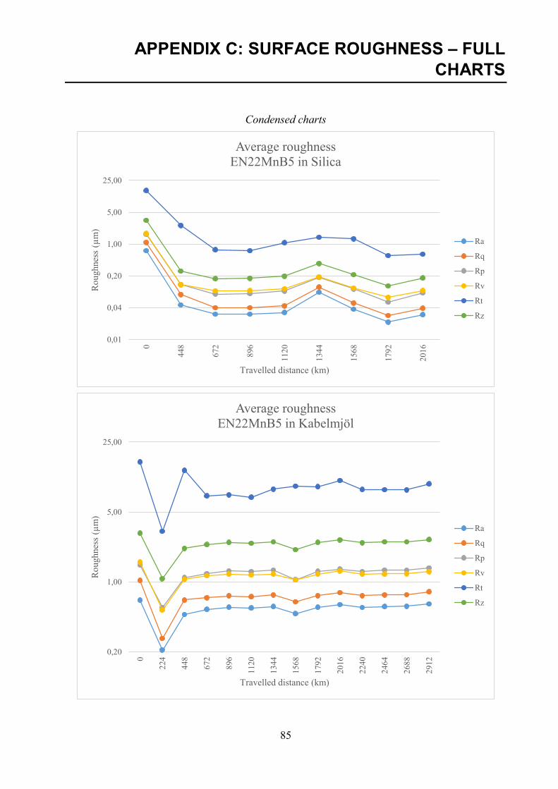
85
APPENDIX C: SURFACE ROUGHNESS – FULL
CHARTS
Condensed charts
0,01
0,04
0,20
1,00
5,00
25,00
0
448
672
896
112
0
134
4
156
8
179
2
201
6
Ro
ughnes
s (µ
m)
Travelled distance (km)
Average roughness
EN22MnB5 in Silica
Ra
Rq
Rp
Rv
Rt
Rz
0,20
1,00
5,00
25,00
0
224
448
672
896
112
0
134
4
156
8
179
2
201
6
224
0
246
4
268
8
291
2
Ro
ughnes
s (µ
m)
Travelled distance (km)
Average roughness
EN22MnB5 in Kabelmjöl
Ra
Rq
Rp
Rv
Rt
Rz

86
0,20
1,00
5,00
25,00
0
224
448
672
896
112
0
134
4
156
8
179
2
201
6
224
0
246
4
268
8
291
2
Ro
ughnes
s (µ
m)
Travelled distance (km)
Average roughness
1559-40+50% 4590 in Kabelmjöl
Ra
Rq
Rp
Rv
Rt
Rz
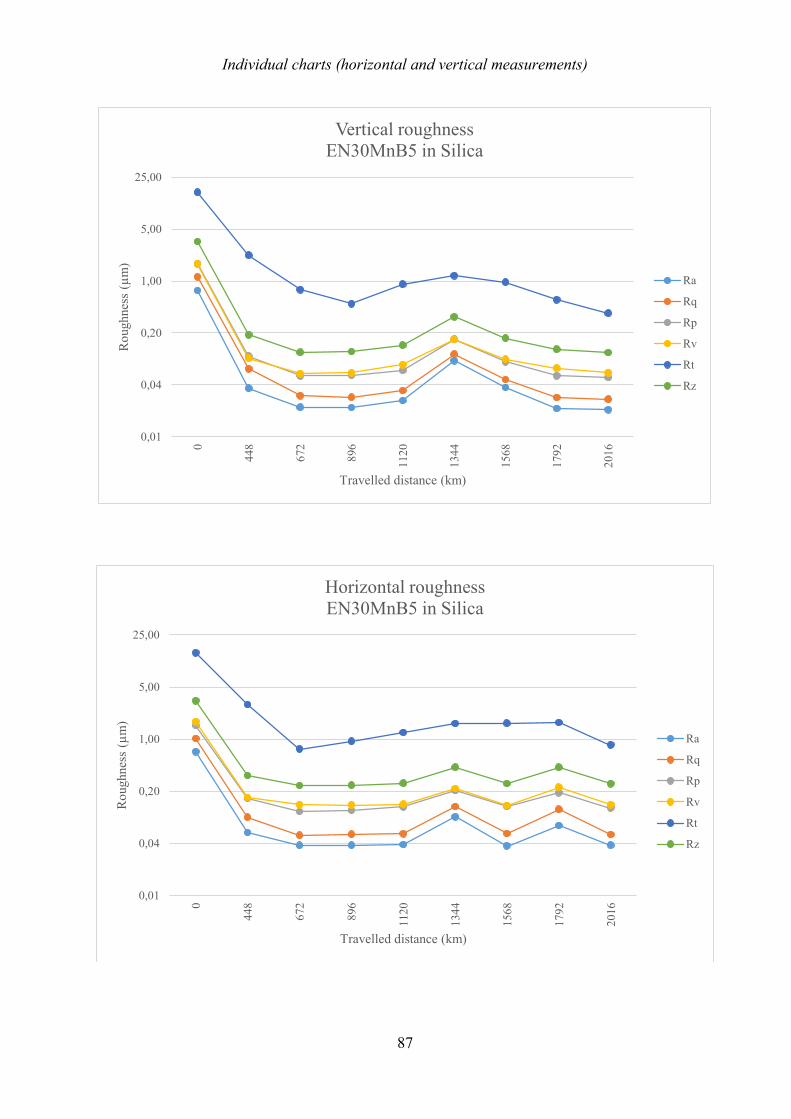
87
Individual charts (horizontal and vertical measurements)
0,01
0,04
0,20
1,00
5,00
25,00
0
448
672
896
112
0
134
4
156
8
179
2
201
6
Ro
ughnes
s (µ
m)
Travelled distance (km)
Vertical roughness
EN30MnB5 in Silica
Ra
Rq
Rp
Rv
Rt
Rz
0,01
0,04
0,20
1,00
5,00
25,00
0
448
672
896
112
0
134
4
156
8
179
2
201
6
Ro
ughnes
s (µ
m)
Travelled distance (km)
Horizontal roughness
EN30MnB5 in Silica
Ra
Rq
Rp
Rv
Rt
Rz

88
0,04
0,20
1,00
5,00
25,00
0
224
448
672
896
112
0
134
4
156
8
179
2
201
6
224
0
246
4
268
8
291
2
Ro
ughnes
s (µ
m)
Travelled distance (km)
Vertical roughness
EN30MnB5 in Kabelmjöl
Ra
Rq
Rp
Rv
Rt
Rz
0,20
1,00
5,00
25,00
0
224
448
672
896
112
0
134
4
156
8
179
2
201
6
224
0
246
4
268
8
291
2
Ro
ughnes
s (µ
m)
Travelled distance (km)
Horizontal roughness
EN30MnB5 in Kabelmjöl
Ra
Rq
Rp
Rv
Rt
Rz

89
0,20
1,00
5,00
25,00
0
224
448
672
896
112
0
134
4
156
8
179
2
201
6
224
0
246
4
268
8
291
2
Ro
ughnes
s (µ
m)
Travelled distance (km)
Vertical roughness
1559-40+50% 4590 in Kabelmjöl
Ra
Rq
Rp
Rv
Rt
Rz
0,20
1,00
5,00
25,00
0
224
448
672
896
112
0
134
4
156
8
179
2
201
6
224
0
246
4
268
8
291
2
Ro
ughnes
s (µ
m)
Travelled distance (km)
Horizontal roughness
1559-40+50% 4590 in Kabelmjöl
Ra
Rq
Rp
Rv
Rt
Rz

90
EN 22MnB5 in Silica sand
Vertical measurements (along Z-Axis)
Horizontal measurements (along X-Axis)
R a R q R p R v R t R z R a R q R p R v R t R z R a R q R p R v R t R z R a R q R p R v R t R z R a R q R p R v R t R z
0.6186 0.9582 1.3921 1.4184 15.7729 2.8104 0.0334 0.0738 0.0995 0.0877 3.7370 0.1872 0.0218 0.0310 0.0632 0.0644 1.0963 0.1276 0.0217 0.0298 0.0637 0.0627 0.5208 0.1264 0.0188 0.0258 0.0534 0.0589 0.5899 0.1123
0.8542 1.3297 2.0357 1.8830 17.5980 3.9187 0.0361 0.0579 0.1004 0.0921 1.8912 0.1925 0.0203 0.0275 0.0570 0.0584 0.5219 0.1154 0.0204 0.0277 0.0564 0.0600 0.5231 0.1164 0.0202 0.0298 0.0562 0.0650 1.4407 0.1212
0.7870 1.2507 1.8037 1.7955 15.5138 3.5991 0.0433 0.0921 0.1206 0.1038 2.8860 0.2244 0.0199 0.0323 0.0543 0.0557 1.2729 0.1100 0.0204 0.0283 0.0588 0.0592 0.6000 0.1179 0.0200 0.0282 0.0507 0.0622 0.4715 0.1129
0.7979 1.2039 1.7778 1.8153 15.7203 3.5931 0.0356 0.0561 0.0914 0.0908 1.5019 0.1821 0.0201 0.0272 0.0495 0.0554 0.4107 0.1049 0.0198 0.0272 0.0529 0.0580 0.4103 0.1110 0.0213 0.0292 0.0511 0.0638 0.5862 0.1149
0.6612 0.9342 1.5838 1.4986 13.4215 3.0824 0.0318 0.0472 0.0755 0.0805 1.1130 0.1560 0.0179 0.0250 0.0401 0.0493 0.5135 0.0894 0.0168 0.0229 0.0387 0.0493 0.4065 0.0881 0.0421 0.0541 0.1015 0.1235 1.4429 0.2250
Avg 0.7438 1.1353 1.7186 1.6822 # # # # 3.4007 0.0360 0.0654 0.0975 0.0910 2.2258 0.1884 0.0200 0.0286 0.0528 0.0566 0.7631 0.1095 0.0198 0.0272 0.0541 0.0578 0.4921 0.1120 0.0245 0.0334 0.0626 0.0747 0.9062 0.1373
D ay 4
Line
1
2
D ay 0 D ay 2 D ay 3 D ay 5
3
4
5
R a R q R p R v R t R z R a R q R p R v R t R z R a R q R p R v R t R z R a R q R p R v R t R z
0.0207 0.0282 0.0633 0.0601 0.6313 0.1234 0.0179 0.0276 0.0502 0.0547 2.0697 0.1049 0.0201 0.0279 0.0539 0.0633 0.5708 0.1172 0.0183 0.0249 0.0518 0.0556 0.3534 0.1074
0.0221 0.0304 0.0672 0.0650 0.4784 0.1322 0.0184 0.0266 0.0458 0.0598 0.8422 0.1056 0.0201 0.0283 0.0542 0.0644 0.6594 0.1186 0.0198 0.0273 0.0541 0.0633 0.5023 0.1174
0.0193 0.0270 0.0560 0.0585 0.8169 0.1145 0.0164 0.0233 0.0446 0.0512 0.6088 0.0959 0.0183 0.0256 0.0486 0.0598 0.5706 0.1084 0.0186 0.0258 0.0507 0.0580 0.5805 0.1086
0.0334 0.0413 0.0753 0.0788 0.5297 0.1541 0.0604 0.0717 0.1166 0.1172 0.5226 0.2337 0.0176 0.0249 0.0477 0.0555 0.4835 0.1032 0.0183 0.0254 0.0533 0.0554 0.0421 0.1087
0.3264 0.3918 0.5592 0.5527 3.4372 1.1119 0.0715 0.0856 0.1495 0.1613 0.7829 0.3109 0.0201 0.0286 0.0600 0.0935 0.5035 0.1535 0.0174 0.0245 0.0427 0.0581 0.3725 0.1008
0.0844 0.1037 0.1642 0.1630 1.1787 0.3272 0.0369 0.0470 0.0813 0.0888 0.9652 0.1702 0.0192 0.0271 0.0529 0.0673 0.5576 0.1202 0.0185 0.0256 0.0505 0.0581 0.3702 0.1086
D ay 8 D ay 9D ay 6 D ay 7
R a R q R p R v R t R z R a R q R p R v R t R z R a R q R p R v R t R z R a R q R p R v R t R z R a R q R p R v R t R z
0.5181 0.7839 1.1226 1.8832 10.1111 3.0058 0.0956 0.1235 0.3045 0.3059 1.1733 0.6104 0.0763 0.1020 0.2249 0.3078 1.0772 0.5327 0.0659 0.0884 0.2056 0.2710 1.0047 0.4766 0.0738 0.1011 0.2534 0.2938 1.3638 0.5472
0.8632 1.2138 2.0617 2.1472 16.1639 4.2089 0.0769 0.1071 0.2269 0.2395 2.4897 0.4665 0.0555 0.0774 0.1759 0.2094 1.1433 0.3853 0.0555 0.0779 0.1826 0.2155 1.2699 0.3981 0.0610 0.0848 0.2069 0.2311 1.1940 0.4381
0.6827 1.0413 1.4799 1.6035 12.3254 3.0834 0.0534 0.0994 0.1357 0.1516 5.0895 0.2873 0.0309 0.0434 0.0810 0.0942 0.6503 0.1752 0.0333 0.0512 0.0903 0.0962 1.2817 0.1865 0.0321 0.0505 0.0963 0.0961 2.8889 0.1923
0.6824 1.0482 1.4815 1.6352 14.9203 3.1167 0.0428 0.0678 0.1068 0.1149 2.0666 0.2217 0.0264 0.0357 0.0671 0.0745 0.6563 0.1416 0.0250 0.0352 0.0672 0.0762 0.5600 0.1434 0.0293 0.0393 0.0811 0.0818 0.7012 0.1629
0.6854 1.0531 1.5827 1.5782 18.1018 3.1609 0.0334 0.0545 0.0936 0.0885 2.7305 0.1821 0.0200 0.0275 0.0519 0.0573 0.4178 0.1092 0.0212 0.0292 0.0594 0.0613 0.5684 0.1207 0.0186 0.0258 0.0558 0.0540 0.7806 0.1098
0.6348 0.9717 1.5007 1.4129 14.2256 2.9136 0.0320 0.0845 0.0889 0.0801 3.8039 0.1689 0.0156 0.0207 0.0417 0.0452 0.4622 0.0869 0.0253 0.0334 0.0606 0.0623 0.8989 0.1230 0.0154 0.0207 0.0456 0.0440 0.4551 0.0896
0.6778 1.0187 1.5382 1.7100 # # # # 3.2482 0.0557 0.0895 0.1594 0.1634 2.8923 0.3228 0.0375 0.0511 0.1071 0.1314 0.7345 0.2385 0.0377 0.0526 0.1110 0.1304 0.9306 0.2414 0.0384 0.0537 0.1232 0.1335 1.2306 0.2567Avg
1
2
3
4
5
6
D ay 3
Line
D ay 0 D ay 2 D ay 5D ay 4
R a R q R p R v R t R z R a R q R p R v R t R z R a R q R p R v R t R z R a R q R p R v R t R z
0.0818 0.1108 0.2758 0.3164 1.2089 0.5921 0.0814 0.1104 0.2938 0.3059 1.1895 0.5997 0.1266 0.2246 0.3121 0.3799 3.0292 0.6920 0.0770 0.1030 0.2486 0.2979 1.3506 0.5465
0.0562 0.0808 0.1885 0.2260 1.3660 0.4145 0.0552 0.0793 0.1995 0.2064 1.3897 0.4059 0.0529 0.0736 0.1742 0.2108 0.9400 0.3850 0.0613 0.0848 0.2024 0.2282 1.1698 0.4306
0.0308 0.0444 0.0905 0.0947 0.7782 0.1852 0.0284 0.0405 0.0864 0.0850 0.5516 0.1714 0.0290 0.0439 0.0843 0.0900 1.0264 0.1743 0.0300 0.0441 0.0919 0.0916 0.8232 0.1835
0.3406 0.4619 0.5729 0.5685 5.0829 1.1414 0.0242 0.0467 0.0729 0.0757 5.0125 0.1486 0.0252 0.0370 0.0758 0.0759 0.7932 0.1517
0.0186 0.0257 0.0489 0.0548 0.4829 0.1037 0.0178 0.0260 0.0537 0.0533 0.8362 0.1070 0.0184 0.0260 0.0546 0.0527 0.5413 0.1073
0.0146 0.0203 0.0430 0.0418 0.8123 0.0848 0.0146 0.0203 0.0449 0.0409 0.8177 0.0858 0.0149 0.0196 0.0420 0.0423 0.3131 0.0844
0.0904 0.1240 0.2033 0.2170 1.6219 0.4203 0.0369 0.0539 0.1252 0.1279 1.6329 0.2531 0.0695 0.1140 0.1902 0.2269 1.6652 0.4171 0.0378 0.0524 0.1192 0.1314 0.8319 0.2507
D ay 8 D ay 9D ay 7D ay 6

91
EN 22MnB5 in Kabelmjöl sand
Vertical measurements (along Z-Axis)
Horizontal measurements (along X-Axis)
R a R q R p R v R t R z R a R q R p R v R t R z R a R q R p R v R t R z R a R q R p R v R t R z R a R q R p R v R t R z
0.7671 1.2002 1.6735 1.7569 15.6213 3.4304 0.1453 0.1950 0.3940 0.3414 2.5246 0.7354 0.3678 0.5131 0.8272 0.8137 13.5190 1.6409 0.4506 0.5864 0.9924 0.9962 6.7788 1.9886 0.4820 0.6282 1.0471 1.0698 7.8636 2.1170
0.7749 1.2500 1.6431 1.8110 20.7478 3.4540 0.1440 0.1957 0.3913 0.3392 2.7497 0.7306 0.3723 0.5336 0.8487 0.8720 10.9663 1.7206 0.4752 0.6305 1.0189 1.0812 8.7623 2.1001 0.4653 0.6097 0.9969 1.0193 6.3871 2.0162
0.7046 1.1840 1.5865 1.6459 21.8822 3.2324 0.1449 0.1920 0.3855 0.3389 2.3574 0.7243 0.3497 0.4758 0.7875 0.7910 8.1470 1.5785 0.4625 0.6059 0.9764 1.0332 7.0360 2.0097 0.4544 0.5903 0.9857 1.0151 5.9648 2.0008
0.6751 1.0740 1.5517 1.5730 16.8704 3.1247 0.1507 0.1984 0.3949 0.3574 2.3264 0.7523 0.3233 0.4280 0.7189 0.7260 6.9921 1.4449 0.4549 0.6053 0.9677 1.0343 7.3074 2.0020 0.4687 0.6191 1.0286 1.0523 7.7164 2.0809
0.4833 0.7074 1.1042 1.3440 10.1798 2.4483 0.1585 0.2079 0.4052 0.3788 2.9260 0.7840 0.3297 0.4277 0.7550 0.7483 4.7394 1.5033 0.4626 0.6041 1.0031 1.0156 5.7455 2.0187 0.4777 0.6240 1.0409 1.0094 5.8586 2.0503
Avg 0.6810 1.0831 1.5118 1.6262 # # # # 3.1380 0.1487 0.1978 0.3942 0.3511 2.5768 0.7453 0.3486 0.4756 0.7875 0.7902 8.8728 1.5776 0.4612 0.6064 0.9917 1.0321 7.1260 2.0238 0.4696 0.6143 1.0198 1.0332 6.7581 2.0530
4
5
3
D ay 3 D ay 4
1
2
Line
D ay 0 D ay 1 D ay 2
R a R q R p R v R t R z R a R q R p R v R t R z R a R q R p R v R t R z R a R q R p R v R t R z R a R q R p R v R t R z
0.4708 0.6132 1.0109 1.0175 6.5142 2.0283 0.4905 0.6419 1.0718 1.0942 6.3085 2.1660 0.5276 0.6981 1.1746 1.1406 10.9093 2.3152 0.5300 0.7019 1.1744 1.1500 11.4593 2.3244 0.5534 0.7379 1.2083 1.1937 12.0374 2.4020
0.4524 0.5958 1.0173 1.0078 6.0707 2.0251 0.4726 0.6282 1.0473 1.0326 9.0613 2.0799 0.4634 0.6072 1.0045 1.0077 12.6618 2.0122 0.4977 0.6525 1.0856 1.1014 6.8801 2.1870 0.5152 0.6772 1.1098 1.1063 10.1579 2.2161
0.4564 0.5938 1.0130 1.0003 6.0279 2.0133 0.4950 0.6508 1.0850 1.0869 7.2393 2.1719 0.4652 0.6044 1.0081 1.0192 6.2216 2.0272 0.4723 0.6190 1.0229 1.0467 7.7778 2.0697 0.5353 0.7308 1.1568 1.1653 12.5438 2.3221
0.4524 0.5893 1.0006 0.9938 5.8134 1.9944 0.4807 0.6309 1.0642 1.0287 8.8512 2.0929 0.4667 0.6130 1.0242 1.0189 6.4718 2.0430 0.4874 0.6343 1.0432 1.0709 6.4818 2.1140 0.5237 0.6978 1.1214 1.1584 11.5922 2.2798
0.4801 0.6263 1.0424 1.0496 5.8234 2.0920 0.5071 0.6692 1.1305 1.1203 7.5390 2.2508 0.4732 0.6174 1.0265 1.0570 5.9882 2.0835 0.5099 0.6832 1.1233 1.1139 9.2226 2.2372
0.4624 0.6037 1.0168 1.0138 6.0499 2.0306 0.4892 0.6442 1.0798 1.0725 7.7999 2.1523 0.4807 0.6307 1.0529 1.0466 9.0661 2.0994 0.4921 0.6450 1.0705 1.0852 7.7174 2.1557 0.5275 0.7054 1.1439 1.1475 11.1108 2.2914
D ay 8 D ay 9D ay 5 D ay 6 D ay 7
R a R q R p R v R t R z R a R q R p R v R t R z R a R q R p R v R t R z R a R q R p R v R t R z
0.5402 0.7467 1.2341 1.1925 11.6073 2.4265 0.5364 0.7135 1.1597 1.1766 10.0116 2.3363 0.5180 0.6841 1.1467 1.1257 9.0253 2.2724 0.5142 0.6828 1.1623 1.1161 7.9032 2.2784
0.4984 0.6651 1.0757 1.1284 9.5299 2.2041 0.5053 0.6656 1.0885 1.0994 7.6124 2.1879 0.4998 0.6705 1.0748 1.0994 8.3827 2.1742 0.5155 0.6764 1.1077 1.1521 7.1642 2.2598
0.4710 0.6179 1.0153 1.0297 8.2277 2.0450 0.4880 0.6440 1.0548 1.0820 9.9772 2.1368 0.4820 0.6250 1.0318 1.0541 7.1805 2.0859 0.5140 0.6825 1.1163 1.1238 8.4014 2.2401
0.4632 0.6101 0.9973 1.0339 7.9648 2.0312 0.4866 0.6363 1.0487 1.0489 6.6745 2.0976 0.4783 0.6311 1.0363 1.0323 8.2137 2.0687 0.5028 0.6637 1.0842 1.1110 7.5373 2.1952
0.4537 0.5898 0.9985 0.9553 5.7464 1.9538 0.4791 0.6225 1.0213 1.0279 6.4375 2.0491 0.4710 0.6158 1.0062 1.0121 7.3497 2.0183 0.4963 0.6539 1.0641 1.0724 6.9318 2.1365
0.4853 0.6459 1.0642 1.0680 8.6152 2.1321 0.4991 0.6564 1.0746 1.0870 8.1426 2.1615 0.4898 0.6453 1.0592 1.0647 8.0304 2.1239 0.5086 0.6719 1.1069 1.1151 7.5876 2.2220
D ay 13D ay 10 D ay 12D ay 11
R a R q R p R v R t R z R a R q R p R v R t R z R a R q R p R v R t R z R a R q R p R v R t R z R a R q R p R v R t R z
0.6313 0.8744 1.5537 1.6307 8.3486 3.1843 0.4109 0.5266 1.1148 1.0859 4.3200 2.2007 0.5508 0.7151 1.4007 1.3286 6.9816 2.7293 0.4851 0.6391 1.2145 1.0758 5.1338 2.2904 0.6512 0.8437 1.6064 1.4277 6.3843 3.0341
0.6038 0.8720 1.4157 1.6518 10.8705 3.0675 0.3458 0.4455 0.9119 0.9708 4.7826 1.8827 0.5678 0.7401 1.4580 1.3123 8.1281 2.7703 0.6563 0.8392 1.5952 1.4920 6.8372 3.0871 0.6477 0.8320 1.6190 1.4288 7.3167 3.0478
0.6451 0.9905 1.4328 1.5847 14.6882 3.0175 0.2485 0.3279 0.6500 0.6245 4.6369 1.2746 0.7389 1.2437 1.7157 1.6200 29.2545 3.3357 0.6365 0.8304 1.4981 1.3202 9.3035 2.8183 0.6645 0.8651 1.5391 1.3389 7.8674 2.8779
0.7061 1.1096 1.5669 1..668 16.2456 3.2349 0.2243 0.2920 0.5874 0.5600 3.1092 1.1474 0.5128 0.6930 1.1943 1.1163 19.5369 2.3105 0.6185 0.8012 1.4323 1.2821 7.9823 2.7144 0.6329 0.8166 1.4589 1.3161 9.8136 2.7750
0.5895 0.9872 1.3403 1.3593 17.2620 2.6996 0.1952 0.2552 0.5252 0.4843 3.3422 1.0095 0.5853 0.7776 1.3373 1.2173 15.4049 2.5546 0.6113 0.7832 1.4088 1.2312 7.7482 2.6400 0.6417 0.8272 1.4986 1.2958 8.8040 2.7944
0.6058 1.0514 1.3360 1.3691 19.9260 2.7051 0.1804 0.2338 0.4773 0.4472 2.8522 0.9246 0.6258 0.8706 1.3759 1.3712 23.8557 2.7470 0.6045 0.7754 1.4046 1.2282 7.0289 2.6327
0.6303 0.9809 1.4409 1.5191 # # # # 2.9848 0.2675 0.3468 0.7111 0.6955 3.8405 1.4066 0.5969 0.8400 1.4137 1.3276 # # # # 2.7412 0.6020 0.7781 1.4256 1.2716 7.3390 2.6972 0.6476 0.8369 1.5444 1.3615 8.0372 2.9058Avg
1
2
3
4
5
D ay 4
6
Line
D ay 0 D ay 1 D ay 2 D ay 3
R a R q R p R v R t R z R a R q R p R v R t R z R a R q R p R v R t R z R a R q R p R v R t R z R a R q R p R v R t R z
0.6345 0.8158 1.5449 1.3943 5.5601 2.9392 0.5484 0.7148 1.2980 1.2005 5.3164 2.4984 0.5676 0.7228 1.3695 1.2757 5.2949 2.6452 0.5798 0.7384 1.4082 1.4748 5.5137 2.8830
0.6950 0.8923 1.6634 1.5345 11.0056 3.1979 0.6768 0.8930 1.7285 1.4526 10.1735 3.1811 0.6279 0.8153 1.5903 1.3895 7.3860 2.9798 0.6378 0.8310 1.5288 1.4609 8.5543 2.9897
0.6260 0.8026 1.4707 1.2783 6.3522 2.7490 0.6608 0.8631 1.5290 1.3322 9.4688 2.8611 0.6214 0.8207 1.4625 1.2847 17.6611 2.7472 0.6831 0.9011 1.5825 1.4093 11.4922 2.9864
0.6222 0.8012 1.4581 1.2634 8.4385 2.7215 0.6759 0.8849 1.6124 1.3570 10.7959 2.9694 0.6506 0.8413 1.5183 1.3292 9.1032 2.8475 0.6695 0.8710 1.5330 1.3769 10.4875 2.9099
0.6418 0.8250 1.5079 1.2889 7.5809 2.7968 0.6446 0.8354 1.5325 1.3054 8.9661 2.8379 0.6505 0.8369 1.5045 1.3139 9.1445 2.8184 0.6859 0.8965 1.5793 1.4025 10.7992 2.9819
0.6055 0.7770 1.4076 1.2212 8.9992 2.6289 0.6564 0.8474 1.5462 1.3022 10.0288 2.8484 0.6241 0.8120 1.4580 1.2911 12.2786 2.7491 0.6881 0.8996 1.5901 1.4220 10.2083 3.0121
0.6375 0.8190 1.5088 1.3301 7.9894 2.8389 0.6438 0.8398 1.5411 1.3250 9.1249 2.8661 # # # # # # # # # # # # # # # # # # # # # # # # 0.6237 0.8082 1.4839 1.3140 # # # # 2.7979 0.6574 0.8563 1.5370 1.4244 9.5092 2.9605
D ay 6D ay 5 D ay 7 D ay 8 D ay 9
R a R q R p R v R t R z R a R q R p R v R t R z R a R q R p R v R t R z R a R q R p R v R t R z
0.4452 0.5789 1.0318 1.0965 6.6498 2.1283 0.5675 0.7462 1.5400 1.2353 8.2826 2.7753 0.5754 0.7507 1.3758 1.2421 6.8252 2.6179 0.6816 0.8715 1.7590 1.4688 5.9746 3.2279
0.6676 0.8637 1.6034 1.5053 7.9523 3.1087 0.6326 0.8234 1.5715 1.3862 8.6462 2.9576 0.6729 0.8742 1.6911 1.4641 7.8785 3.1552 0.6742 0.8831 1.6341 1.5186 12.5628 3.1526
0.6670 0.8569 1.5404 1.3528 8.5461 2.8933 0.6294 0.8148 1.4886 1.2608 8.0289 2.7494 0.6654 0.8630 1.5541 1.3472 9.6947 2.9013 0.8049 1.1576 1.7621 1.4646 22.5171 3.2267
0.6718 0.8712 1.5750 1.3330 9.4405 2.9081 0.6731 0.8724 1.5876 1.3476 7.9603 2.9352 0.6641 0.8633 1.5714 1.3390 8.9727 2.9104 0.6746 0.8731 1.5968 1.3676 9.1512 2.9644
0.6659 0.8559 1.5327 1.3444 8.3002 2.8771 0.6729 0.8581 1.5683 1.3580 8.4782 2.9262 0.6710 0.8671 1.5868 1.3589 8.5769 2.9457 0.6635 0.8648 1.5768 1.3397 8.9366 2.9165
0.6319 0.8173 1.4845 1.2893 7.8553 2.7739 0.6465 0.8402 1.5424 1.3027 9.7264 2.8451 0.6551 0.8458 1.5308 1.3389 9.4290 2.8696 0.6716 0.8699 1.5984 1.3472 9.6383 2.9456
0.6249 0.8073 1.4613 1.3202 8.1240 2.7816 0.6370 0.8259 1.5497 1.3151 8.5204 2.8648 0.6507 0.8440 1.5517 1.3484 8.5628 2.9000 0.6951 0.9200 1.6545 1.4178 # # # # 3.0723
D ay 12 D ay 13D ay 11D ay 10

92
1559-40+50% 4590 in Kabelmjöl sand
Vertical measurements (along Z-Axis)
Horizontal measurements (along X-Axis)
R a R q R p R v R t R z R a R q R p R v R t R z R a R q R p R v R t R z R a R q R p R v R t R z R a R q R p R v R t R z
1.1427 1.6459 2.5378 2.5469 19.0314 5.0847 0.3059 0.4529 0.7090 0.7181 9.6996 1.4271 0.4707 0.6275 1.0849 1.0903 11.7209 2.1752 0.5122 0.6864 1.1541 1.1575 9.9946 2.3115 0.6383 0.8686 1.4614 1.4793 10.6236 2.9407
1.2310 1.7609 2.7681 2.7222 20.0717 5.4903 0.2872 0.4301 0.6455 0.6884 10.3590 1.3338 0.5072 0.6839 1.1622 1.1629 9.3373 2.3251 0.6154 0.8666 1.3516 1.4203 10.9818 2.7719 0.5907 0.8058 1.3306 1.3504 10.9362 2.6809
1.2896 1.8503 2.7792 2.8856 20.3323 5.6648 0.2776 0.4300 0.6021 0.6629 8.9920 1.2650 0.5393 0.7655 1.1961 1.2308 11.6757 2.4269 0.5282 0.7411 1.1824 1.1990 13.4308 2.3814 0.6073 0.8453 1.3565 1.3760 12.5002 2.7325
1.3293 1.9033 2.7099 3.0120 20.4186 5.7220 0.2988 0.4554 0.6528 0.6935 7.5194 1.3463 0.5375 0.7518 1.2272 1.2372 9.0597 2.4644 0.6177 0.8603 1.3646 1.3590 12.4162 2.7237 0.6344 0.8719 1.4128 1.4212 10.8410 2.8340
0.9595 1.4046 1.9592 2.2065 18.6237 4.1658 0.3858 0.6321 0.8171 0.8611 12.1319 1.6782 0.5961 0.8331 1.2885 1.3656 13.5714 2.6542 0.6968 0.9690 1.5133 1.5935 11.5194 3.1068 0.6936 0.9346 1.5078 1.5184 9.1627 3.0263
Avg 1.1904 1.7130 2.5508 2.6746 # # # # 5.2255 0.3111 0.4801 0.6853 0.7248 9.7404 1.4101 0.5302 0.7324 1.1918 1.2174 # # # # 2.4092 0.5941 0.8247 1.3132 1.3459 # # # # 2.6591 0.6329 0.8652 1.4138 1.4291 # # # # 2.8429
Line
D ay 0 D ay 1 D ay 2 D ay 3 D ay 4
4
1
2
3
5
R a R q R p R v R t R z R a R q R p R v R t R z R a R q R p R v R t R z R a R q R p R v R t R z R a R q R p R v R t R z
0.6423 0.8494 1.4733 1.4191 10.6418 2.8924 0.6762 0.8953 1.5524 1.5121 9.8634 3.0645 0.6632 0.8803 1.5581 1.4534 11.2157 3.0115 0.6727 0.9080 1.5576 1.5075 12.6616 3.0651 0.6541 0.8876 1.5203 1.4393 10.7568 2.9596
0.6388 0.8720 1.4462 1.4388 12.1883 2.8850 0.6251 0.8498 1.4198 1.4107 12.7102 2.8305 0.6365 0.8540 1.4926 1.4049 11.5226 2.8974 0.6343 0.8500 1.4596 1.4061 9.0963 2.8656 0.6270 0.8342 1.4477 1.3806 9.6985 2.8283
0.6819 0.9437 1.5183 1.5501 14.5914 3.0684 0.6213 0.8609 1.4011 1.4093 12.3998 2.8104 0.6493 0.8920 1.4596 1.4463 13.8604 2.9059 0.6585 0.9021 1.4649 1.4946 12.5510 2.9595 0.6227 0.8499 1.4358 1.3867 11.1058 2.8225
0.7022 0.9806 1.5448 1.5836 12.1550 3.1284 0.6868 0.9381 1.5293 1.5609 10.9824 3.0902 0.6647 0.9112 1.4940 1.5066 12.0714 3.0006 0.6529 0.8989 1.4876 1.4436 11.4629 2.9312 0.6640 0.8947 1.4941 1.4689 13.9465 2.9630
0.7380 1.0152 1.6880 1.7118 15.5179 3.3998 0.6971 0.9642 1.5469 1.5829 11.8443 3.1298 0.7084 0.9932 1.5598 1.5721 11.6914 3.1320 0.6424 0.8822 1.4585 1.4142 11.7903 2.8728 0.5868 0.7814 1.3068 1.2976 9.2851 2.6043
0.6806 0.9322 1.5341 1.5407 # # # # 3.0748 0.6613 0.9017 1.4899 1.4952 # # # # 2.9851 0.6644 0.9061 1.5128 1.4767 # # # # 2.9895 0.6522 0.8882 1.4856 1.4532 11.5124 2.9388 0.6309 0.8496 1.4409 1.3946 # # # # 2.8355
D ay 5 D ay 6 D ay 7 D ay 8 D ay 9
R a R q R p R v R t R z R a R q R p R v R t R z R a R q R p R v R t R z R a R q R p R v R t R z
0.6279 0.8520 1.4434 1.4230 10.9569 2.8664 0.6528 0.8649 1.4587 1.4580 10.8946 2.9167 0.6106 0.8216 1.3879 1.3844 9.2598 2.7723
0.6163 0.8439 1.4057 1.4005 11.4405 2.8062 0.6164 0.8271 1.3856 1.3964 9.0632 2.7820 0.5706 0.7840 1.3084 1.3217 9.1416 2.6301
0.6317 0.8588 1.4692 1.4219 11.9632 2.8911 0.5971 0.8133 1.3582 1.3690 12.5729 2.7272 0.5987 0.8193 1.3916 1.3629 12.6743 2.7546
0.5841 0.7848 1.3370 1.2669 9.9023 2.6039 0.6050 0.8232 1.3916 1.3566 9.7962 2.7482 0.6057 0.8516 1.3871 1.3621 15.5569 2.7492
0.6139 0.8521 1.3662 1.3768 12.2119 2.7429 0.6311 0.8474 1.4150 1.4079 10.2938 2.8229 0.5893 0.8153 1.3379 1.3070 12.2915 2.6449
0.6148 0.8383 1.4043 1.3778 # # # # 2.7821 0.6205 0.8352 1.4018 1.3976 # # # # 2.7994 # # # # # # # # # # # # # # # # # # # # # # # # 0.5950 0.8184 1.3626 1.3476 # # # # 2.7102
D ay 12 D ay 13D ay 10 D ay 11
R a R q R p R v R t R z R a R q R p R v R t R z R a R q R p R v R t R z R a R q R p R v R t R z R a R q R p R v R t R z
0.9210 1.5112 1.9133 2.0797 17.8329 3.9929 0.9158 1.3470 1.5690 1.9748 16.4215 3.5437 1.0455 1.3696 1.7597 2.5141 10.5339 4.2738 1.0744 1.4468 2.0258 2.4655 12.1056 4.4913 1.0077 1.3045 2.0081 2.3187 9.7093 4.3268
1.1264 1.6486 2.3697 2.8442 17.2197 5.2139 0.5760 0.8325 1.2858 1.4179 11.1467 2.7037 0.7505 1.0215 1.6180 1.7769 11.3492 3.3949 0.7065 0.9575 1.5996 1.6006 12.4451 3.2002 0.7584 1.0234 1.6324 1.7522 10.5759 3.3846
1.0319 1.5504 2.1931 2.3220 17.4429 4.5151 0.4456 0.6390 0.9425 1.0193 8.8428 1.9618 0.6191 0.8872 1.2910 1.3983 12.7328 2.6893 0.6260 0.8699 1.3408 1.4163 11.6205 2.7571 0.6667 0.9271 1.3996 1.5126 14.5649 2.9121
1.1851 1.7001 2.5489 2.6211 19.0845 5.1700 0.4000 0.5770 0.9086 0.8932 10.0083 1.8018 0.5270 0.7449 1.1508 1.2092 14.0012 2.3599 0.5618 0.7831 1.2575 1.3009 16.7318 2.5583 0.6493 0.8872 1.4254 1.4854 13.0031 2.9107
1.3099 1.8278 2.8203 2.8905 18.2815 5.7108 0.3405 0.4723 0.8097 0.7733 8.8753 1.5830 0.5166 0.7207 1.1579 1.1833 11.6793 2.3412 0.4997 0.6673 1.1242 1.1802 9.2665 2.3044 0.6105 0.8252 1.3545 1.3808 12.0429 2.7353
1.4600 1.9649 3.2571 3.0928 21.3103 6.3499 0.2937 0.3804 0.7282 0.6841 4.8856 1.4123 0.5494 0.7461 1.2300 1.2653 11.9604 2.4953 0.5417 0.7200 1.1914 1.2384 10.5455 2.4299 0.5650 0.7430 1.2806 1.2684 9.4611 2.5489
1.1724 1.7005 2.5171 2.6417 # # # # 5.1588 0.4953 0.7080 1.0406 1.1271 # # # # 2.1677 0.6680 0.9150 1.3679 1.5579 # # # # 2.9257 0.6684 0.9074 1.4232 1.5337 12.1192 2.9569 0.7096 0.9517 1.5168 1.6197 # # # # 3.1364
Line
D ay 0 D ay 1 D ay 2 D ay 3 D ay 4
6
Avg
1
2
3
4
5
R a R q R p R v R t R z R a R q R p R v R t R z R a R q R p R v R t R z R a R q R p R v R t R z R a R q R p R v R t R z
1.1151 1.5089 1.8279 2.7583 12.3729 4.5861 0.9529 1.2719 1.7262 2.2959 11.6510 4.0221 0.7318 0.9780 1.4985 1.6020 8.2148 3.1005 1.2407 1.6337 1.9553 2.7981 13.1585 4.7534 0.8497 1.2273 1.4024 1.8830 13.2331 3.2854
0.7558 1.0190 1.7050 1.7160 11.6575 3.4210 0.7964 1.0735 1.7616 1.8156 10.6690 3.5772 0.8531 1.1567 1.7933 1.9367 11.6753 3.7300 0.8454 1.1573 1.8121 1.9881 11.8530 3.8003 0.7637 1.0810 1.6214 1.8128 22.2472 3.4343
0.6958 0.9714 1.5455 1.5209 16.7295 3.0663 0.7409 1.0350 1.6358 1.6665 17.1941 3.3024 0.7281 1.0207 1.5968 1.5727 22.4968 3.1694 0.6791 0.9183 1.5573 1.4737 12.6637 3.0310 0.6674 0.9096 1.5019 1.4419 15.5162 2.9438
0.7217 0.9822 1.5549 1.6178 13.4044 3.1727 0.7159 0.9755 1.5623 1.5665 12.2121 3.1288 0.6979 0.9585 1.5245 1.5030 15.1837 3.0275 0.6854 0.9369 1.5259 1.5235 12.1784 3.0494 0.6727 0.8965 1.5219 1.4658 12.5610 2.9877
0.6932 0.9391 1.5385 1.4934 12.2796 3.0319 0.7071 0.9372 1.5774 1.5275 11.5067 3.1049 0.6848 0.9138 1.5418 1.4801 9.4727 3.0219 0.6706 0.8878 1.5318 1.4504 11.4036 2.9822 0.6924 0.9257 1.6088 1.4693 11.8340 3.0781
0.6498 0.8645 1.4893 1.4497 11.0701 2.9390 0.6831 0.8959 1.5375 1.4758 8.6953 3.0132 0.6523 0.8677 1.5042 1.4026 12.4996 2.9069 0.6161 0.8062 1.4556 1.3413 9.3426 2.7969 0.6269 0.8345 1.4598 1.3518 9.9295 2.8116
0.7719 1.0475 1.6102 1.7594 # # # # 3.3695 0.7661 1.0315 1.6335 1.7246 # # # # 3.3581 0.7247 0.9826 1.5765 1.5829 # # # # 3.1594 0.7896 1.0567 1.6397 1.7625 # # # # 3.4022 0.7121 0.9791 1.5194 1.5708 # # # # 3.0902
D ay 5 D ay 6 D ay 7 D ay 8 D ay 9
R a R q R p R v R t R z R a R q R p R v R t R z R a R q R p R v R t R z R a R q R p R v R t R z
0.9117 1.4072 1.9850 2.0713 20.9037 4.0564 0.6585 0.9457 1.3650 1.5262 12.0818 2.8912 0.7265 1.0166 1.5088 1.6183 10.5542 3.1271
0.7258 0.9788 1.6045 1.6738 11.2965 3.2783 0.7977 1.1143 1.7442 1.8174 20.6794 3.5617 0.6298 0.8300 1.4936 1.4719 10.7276 2.9655
0.6409 0.8578 1.4691 1.3631 9.5565 2.8322 0.6149 0.8171 1.3848 1.3257 10.4170 2.7105 0.6044 0.8137 1.3898 1.2754 10.9094 2.6651
0.6656 0.9028 1.4998 1.4431 11.8696 2.9429 0.6562 0.8792 1.5065 1.4044 11.5079 2.9109 0.7041 0.9487 1.6411 1.5049 12.6351 3.1461
0.6860 0.9198 1.5637 1.4801 11.1899 3.0438 0.6727 0.8946 1.5733 1.4667 11.3547 3.0399 0.6549 0.8680 1.5539 1.3935 9.1314 2.9475
0.6225 0.8317 1.4785 1.3565 13.0016 2.8350 0.6581 0.8729 1.5654 1.4223 10.6526 2.9877 0.6930 0.9110 1.6848 1.4583 9.2098 3.1431
0.7088 0.9830 1.6001 1.5647 # # # # 3.1648 0.6764 0.9206 1.5232 1.4938 # # # # 3.0170 # # # # # # # # # # # # # # # # # # # # # # # # 0.6688 0.8980 1.5453 1.4537 # # # # 2.9991
D ay 13D ay 10 D ay 11 D ay 12

93
APPENDIX D: SURFACE PROFILE – INDIVIDUAL
GRAPHS
Day 0
0 km
Day 2
448 km
Day 5
1120 km
Day 9
2016 km
EN 22MnB5 in Silica - Tip side, vertical sampling
Surface profile of the EN 22MnB5 material in silica sand during 4 different days. A rougher
profile can be observed in Day 0, while it smoothens in the following days.

94
Day 0
0 km
Day 2
448 km
Day 5
1120 km
Day 9
2016 km
EN 22MnB5 in Silica - Tip side, horizontal sampling
A rough surface can be observed in Day 0 (0 km), and it can be observed that the curve
smoothens as time passes, just as the previous figure.

95
Day 0
0 km
Day 1
224 km
Day 5
1120 km
Day 13
2912 km
EN 22MnB5 in Kabelmjöl - Tip side, vertical sampling
Roughness development for EN 22MnB5 in Kabelmjöl sand. A rougher surface can also be
observed in Day 0, and a much smoother surface can be observed in Day 1. However, some
surface imperfection can be observed in Day 5, which could be due to lose oxide layers on the
material.
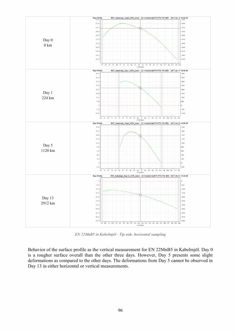
96
Day 0
0 km
Day 1
224 km
Day 5
1120 km
Day 13
2912 km
EN 22MnB5 in Kabelmjöl - Tip side, horizontal sampling
Behavior of the surface profile as the vertical measurement for EN 22MnB5 in Kabelmjöl. Day 0
is a rougher surface overall than the other three days. However, Day 5 presents some slight
deformations as compared to the other days. The deformations from Day 5 cannot be observed in
Day 13 in either horizontal or vertical measurements.

97
Day 0
0 km
Day 1
224 km
Day 5
1120 km
Day 13
2912 km
1559-40+50% 4590 in Kabelmjöl - Tip side, vertical sampling
The right-hand “step” shows where the laser cladding is located close to the tip of the blade. A
rougher, more notorious step can be observed in Day 0. Day 1 (224 km) and Day 5 (1120 km)
both present a smoother step (around the valley area of the step). Finally, Day 13 (2912 km)
presents the smoothest valley and peak of the four profiles. However, the loss of material does
not appear to be very significant, either from the profile measurement or visually.

98
Day 0
0 km
Day 1
224 km
Day 5
1120 km
Day 13
2912 km
1559-40+50% 4590 in Kabelmjöl - Tip side, horizontal sampling
A more notorious step is also observable in Day 0 compared to the rest of the days. Smoother
profiles can be observed as the test advances, meaning that some smoothening of the material
might happen as time passes, or that oxide builds up close to the “valleys” of the cladded parts,
giving a smoother “transition” between both the base material and the carbide cladding.


![[PPT]Abrasive Waterjet Machining - Southern Illinois …scho/index_files/Abrasive Waterjet.ppt · Web viewTitle Abrasive Waterjet Machining Author Academic Computing Last modified](https://img.dokumen.tips/doc/110x75/5aa4961d7f8b9ac8748c252d/pptabrasive-waterjet-machining-southern-illinois-schoindexfilesabrasive.jpg)