Introduction First example Data structures and algorithms Second example

A Simple Finite Element Codewritten in Julia

Bill McLean, UNSW

ANZMC Melbourne December 2014

Introduction First example Data structures and algorithms Second example

Purpose

Required for the computational component of an honours course(3 hours/week for 6 weeks) on finite elements.

Suffices for code to handle

I second-order, linear elliptic PDEs in 2D,

I P1-elements (triangular, degree 1).

Expect students to study the source code to understand FEM,particularly matrix assembly. Should not be a “black box”.

Students also use the code in an assignment.

Introduction First example Data structures and algorithms Second example

Purpose

Required for the computational component of an honours course(3 hours/week for 6 weeks) on finite elements.

Suffices for code to handle

I second-order, linear elliptic PDEs in 2D,

I P1-elements (triangular, degree 1).

Expect students to study the source code to understand FEM,particularly matrix assembly. Should not be a “black box”.

Students also use the code in an assignment.

Introduction First example Data structures and algorithms Second example

Purpose

Required for the computational component of an honours course(3 hours/week for 6 weeks) on finite elements.

Suffices for code to handle

I second-order, linear elliptic PDEs in 2D,

I P1-elements (triangular, degree 1).

Expect students to study the source code to understand FEM,particularly matrix assembly. Should not be a “black box”.

Students also use the code in an assignment.

Introduction First example Data structures and algorithms Second example

Purpose

Required for the computational component of an honours course(3 hours/week for 6 weeks) on finite elements.

Suffices for code to handle

I second-order, linear elliptic PDEs in 2D,

I P1-elements (triangular, degree 1).

Expect students to study the source code to understand FEM,particularly matrix assembly. Should not be a “black box”.

Students also use the code in an assignment.

Introduction First example Data structures and algorithms Second example

Why Julia?

I Modern alternative to Matlab.

I MIT licence and good documentation.

I Cross-platform: Linux, Windows and OS X.

I Easy, student-friendly syntax.

I Fast execution thanks to LLVM.

I Extensive bindings to standard numerical libraries.

Ported code from previous version written in Python.

Introduction First example Data structures and algorithms Second example

Why Julia?

I Modern alternative to Matlab.

I MIT licence and good documentation.

I Cross-platform: Linux, Windows and OS X.

I Easy, student-friendly syntax.

I Fast execution thanks to LLVM.

I Extensive bindings to standard numerical libraries.

Ported code from previous version written in Python.

Introduction First example Data structures and algorithms Second example

Overview of FEM solution process

Geometry description (.geo) file

Mesh description (.msh) file

Postprocessing (.pos) file

Graphical output

Gmsh

Julia script

Gmsh

Introduction First example Data structures and algorithms Second example

Gmsh

C. Geuzaine and J.-F. Remacle. Gmsh: a three-dimensional finiteelement mesh generator with built-in pre- and post-processingfacilities. International Journal for Numerical Methods inEngineering 79(11), pp. 1309–1331, 2009.

I GPL software with comprehensive documentation.

I Cross-platform: Linux, Windows and OS X.

I Fast and robust meshes in 2D and 3D.

I Convenient data format for FEM.

I Extensive visualisation features.

I Reasonably easy to handle simple geometries.

FEM code has no other software dependency.

Introduction First example Data structures and algorithms Second example

Gmsh

C. Geuzaine and J.-F. Remacle. Gmsh: a three-dimensional finiteelement mesh generator with built-in pre- and post-processingfacilities. International Journal for Numerical Methods inEngineering 79(11), pp. 1309–1331, 2009.

I GPL software with comprehensive documentation.

I Cross-platform: Linux, Windows and OS X.

I Fast and robust meshes in 2D and 3D.

I Convenient data format for FEM.

I Extensive visualisation features.

I Reasonably easy to handle simple geometries.

FEM code has no other software dependency.

Introduction First example Data structures and algorithms Second example

Package modules

Gmsh.jl Handles reading and writing of Gmsh data files.

FEM.jl Handles assembly of linear system.

PlanarPoisson.jl Routines to compute element stiffness matrix,element load vector, etc.

How many lines of code?

$ wc *.jl

229 657 6469 FEM.jl

249 823 7850 Gmsh.jl

152 518 4423 PlanarPoisson.jl

630 1998 18742 total

Introduction First example Data structures and algorithms Second example

Package modules

Gmsh.jl Handles reading and writing of Gmsh data files.

FEM.jl Handles assembly of linear system.

PlanarPoisson.jl Routines to compute element stiffness matrix,element load vector, etc.

How many lines of code?

$ wc *.jl

229 657 6469 FEM.jl

249 823 7850 Gmsh.jl

152 518 4423 PlanarPoisson.jl

630 1998 18742 total

Introduction First example Data structures and algorithms Second example

Simple example

−∇2u = 4

u = 0

Introduction First example Data structures and algorithms Second example

Weak formulation and finite element approximation

Sobolev space H10(Ω) consists of those u ∈ L2(Ω) such that ∂xuand ∂yu ∈ L2(Ω), with u = 0 on Ω.Weak solution u ∈ H10(Ω) satisfies∫

Ω

∇u · ∇v =∫Ω

4v for all v ∈ H10(Ω).

Approximate Ω by triangulated domain Ωh.

Finite element space Sh consists of all continuous, piecewise-linearfunctions that vanish on ∂Ωh; thus, Sh ⊆ H10(Ωh).

Finite element solution uh ∈ Sh satisfies∫Ωh

∇uh · ∇v =∫Ωh

4v for all v ∈ Sh.

Introduction First example Data structures and algorithms Second example

Weak formulation and finite element approximation

Sobolev space H10(Ω) consists of those u ∈ L2(Ω) such that ∂xuand ∂yu ∈ L2(Ω), with u = 0 on Ω.Weak solution u ∈ H10(Ω) satisfies∫

Ω

∇u · ∇v =∫Ω

4v for all v ∈ H10(Ω).

Approximate Ω by triangulated domain Ωh.

Finite element space Sh consists of all continuous, piecewise-linearfunctions that vanish on ∂Ωh; thus, Sh ⊆ H10(Ωh).

Finite element solution uh ∈ Sh satisfies∫Ωh

∇uh · ∇v =∫Ωh

4v for all v ∈ Sh.

Introduction First example Data structures and algorithms Second example

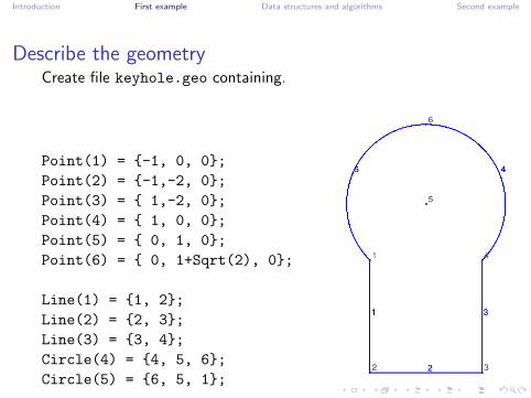
Describe the geometryCreate file keyhole.geo containing.

Point(1) = -1, 0, 0;

Point(2) = -1,-2, 0;

Point(3) = 1,-2, 0;

Point(4) = 1, 0, 0;

Point(5) = 0, 1, 0;

Point(6) = 0, 1+Sqrt(2), 0;

Line(1) = 1, 2;

Line(2) = 2, 3;

Line(3) = 3, 4;

Circle(4) = 4, 5, 6;

Circle(5) = 6, 5, 1;

Introduction First example Data structures and algorithms Second example

Label the domain and boundary

Line Loop(7) = 1, 2, 3, 4, 5;

Plane Surface(1) = 7 ;

Physical Surface("Omega") = 1 ;

Physical Line("Gamma") = 1, 2, 3, 4, 5 ;

Introduction First example Data structures and algorithms Second example

Triangulate the domain

Use Gmsh GUI or CLI to create file keyhole.msh.

Introduction First example Data structures and algorithms Second example

Solver scriptusing Gmsh

using FEM

using PlanarPoisson

mesh = read_msh_file("keyhole.msh")

essential_bc = [ "Gamma" ]

f(x) = 4.0

vp = VariationalProblem(mesh, essential_bc)

add_bilin_form!(vp, "Omega", grad_dot_grad!)

add_lin_functnl!(vp, "Omega", source_times_func!, f)

A, b = assembled_linear_system(vp)

ufree = A \ b

u = complete_soln(ufree, vp)

open("keyhole.pos", "w") do fid

write_format_version(fid)

save_warp_nodal_scalar_field(u, "u", mesh, fid)

end

Introduction First example Data structures and algorithms Second example

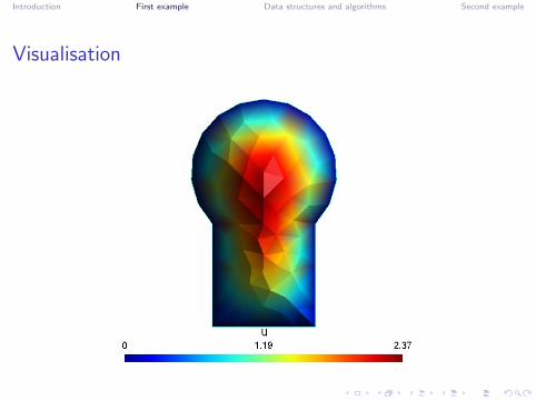
Visualisation

Introduction First example Data structures and algorithms Second example

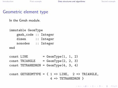
Geometric element type

In the Gmsh module.

immutable GeomType

gmsh_code :: Integer

dimen :: Integer

nonodes :: Integer

end

const LINE = GeomType(1, 1, 2)

const TRIANGLE = GeomType(2, 2, 3)

const TETRAHEDRON = GeomType(4, 3, 4)

const GETGEOMTYPE = 1 => LINE, 2 => TRIANGLE,

4 => TETRAHEDRON

Introduction First example Data structures and algorithms Second example

Mesh data structure

immutable Mesh

coord :: ArrayFloat64, 2

physdim :: DictString, Integer

physnum :: DictString, Integer

physname :: DictInteger, String

elmtype :: DictString, GeomType

elms_of :: DictString, MatrixInteger

nodes_of :: DictString, SetInteger

end

For example,

mesh.coord[:,n] = x, y, z coordinates of nth node,

mesh.elms of["Omega"] =connectivity matrix forelements in Ω.

Introduction First example Data structures and algorithms Second example

FEM data structures

immutable DoF

isfree :: VectorBool

freenode :: VectorInteger

fixednode :: VectorInteger

node2free :: VectorInteger

node2fixed :: VectorInteger

end

immutable VariationalProblem

mesh :: Mesh

dof :: DoF

essential_bc :: VectorASCIIString

bilin_form :: VectorAny

lin_functnl :: VectorAny

ufixed :: VectorFloat64

end

Introduction First example Data structures and algorithms Second example

Inhomogeneous Dirichlet data

function assign_bdry_vals!(vp::VariationalProblem,

name::String, g::Function)

if !(name in vp.essential_bc)

error("$name: not listed in essential_bc")

end

for nd in vp.mesh.nodes_of[name]

i = vp.dof.node2fixed[nd]

x = vp.mesh.coord[:,nd]

vp.ufixed[i] = g(x)

end

end

Introduction First example Data structures and algorithms Second example

Matrix assembly

A = sparse(Int64[], Int64[], Float64[], nofree, nofree)

b = zeros(nofree)

for (name, elm_mat!, coef) in vp.bilin_form

next = assembled_matrix(name, elm_mat!,

coef, mesh, dof)

A += next[:,1:nofree]

if nofixed > 0

b -= next[:,nofree+1:end] * vp.ufixed

end

end

for (name, elm_vec!, f) in vp.lin_functnl

next = assembled_vector(name, elm_vec!, f,

mesh, dof)

b += next

end

Introduction First example Data structures and algorithms Second example

A more complicated example

u = −|x|/2

u = 0

∂u

∂n= −1

∂u

∂n= −1

∂u

∂n= 0

−∇ · (a∇u) = f

a = 1

f = 1

a = 10

f = 4

Introduction First example Data structures and algorithms Second example

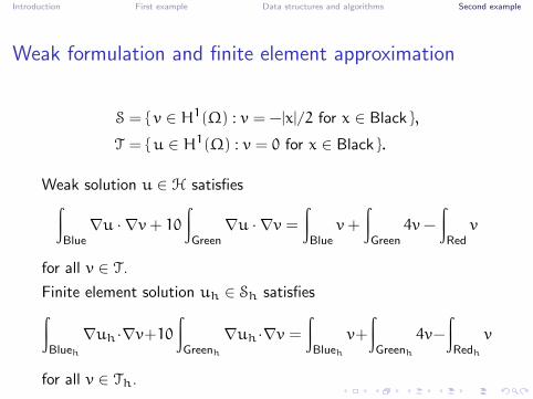
Weak formulation and finite element approximation

S = v ∈ H1(Ω) : v = −|x|/2 for x ∈ Black ,

T = u ∈ H1(Ω) : v = 0 for x ∈ Black .

Weak solution u ∈ H satisfies∫Blue∇u · ∇v+ 10

∫Green

∇u · ∇v =∫Blue

v+

∫Green

4v−

∫Redv

for all v ∈ T.

Finite element solution uh ∈ Sh satisfies∫Blueh

∇uh ·∇v+10∫Greenh

∇uh ·∇v =∫Blueh

v+

∫Greenh

4v−

∫Redh

v

for all v ∈ Th.

Introduction First example Data structures and algorithms Second example

Weak formulation and finite element approximation

S = v ∈ H1(Ω) : v = −|x|/2 for x ∈ Black ,

T = u ∈ H1(Ω) : v = 0 for x ∈ Black .

Weak solution u ∈ H satisfies∫Blue∇u · ∇v+ 10

∫Green

∇u · ∇v =∫Blue

v+

∫Green

4v−

∫Redv

for all v ∈ T.

Finite element solution uh ∈ Sh satisfies∫Blueh

∇uh ·∇v+10∫Greenh

∇uh ·∇v =∫Blueh

v+

∫Greenh

4v−

∫Redh

v

for all v ∈ Th.

Introduction First example Data structures and algorithms Second example

Setting up the variational problem

g(x) = -hypot(x[1],x[2])/2

assign_bdry_vals!(vp, "North", g)

add_bilin_form!(vp, "Major",

grad_dot_grad!, 1.0)

add_lin_functnl!(vp, "Major",

source_times_func!, x->1.0)

add_bilin_form!(vp, "Minor",

grad_dot_grad!, 10.0)

add_lin_functnl!(vp, "Minor",

source_times_func!, x->4.0)

add_lin_functnl!(vp, "East",

bdry_source_times_func!, x->-1.0)

add_lin_functnl!(vp, "West",

bdry_source_times_func!, x->-1.0)

Introduction First example Data structures and algorithms Second example

Visualisation4604 nodes, 9291 triangles.