A Combinatorial Approximation Algorithm for Graph Balancing

with Light Hyper Edges

Chien-Chung Huang1 and Sebastian Ott2

1Chalmers University, Goteborg, Sweden, villars@gmail.com2Max Planck Institute for Informatics, Saarbrucken, Germany, ott@mpi-inf.mpg.de

Abstract

Makespan minimization in restricted assignment (R|pij ∈ {pj ,∞}|Cmax) is a classical prob-lem in the field of machine scheduling. In a landmark paper in 1990 [7], Lenstra, Shmoys, andTardos gave a 2-approximation algorithm and proved that the problem cannot be approximatedwithin 1.5 unless P=NP. The upper and lower bounds of the problem have been essentiallyunimproved in the intervening 25 years, despite several remarkable successful attempts in somespecial cases of the problem [1, 3, 10] recently.

In this paper, we consider a special case called graph-balancing with light hyper edges: jobswith weights in the range of (βW,W ] can be assigned to at most two machines, where 4/7 ≤β < 1, and W is the largest job weight, while there is no restriction on the number of machinesa job can be assigned to if its weight is in the range of (0, βW ]. Our main contribution is a5/3 + β/3 approximation algorithm, thus breaking the barrier of 2 in this special case. Unlikethe several recent works [1, 3, 10] that make use of (configuration)-LPs, our algorithm is purelycombinatorial.

In addition, we consider another special case where jobs have only two possible weights{w,W}, and w < W . Jobs with weight W can be assigned to only two machines, while there isno restriction on the others. For this special case, we give a 1.5-approximation algorithm, thusmatching the general lower bound (indeed the current 1.5 lower bound is established in an evenmore restricted setting). Interestingly, depending on the specific values of w and W , sometimesour algorithm guarantees sub-1.5 approximation ratios.

1 Introduction

Let J be a set of jobs and M a set of machines. Each job j ∈ J has a weight wj and can beassigned to a specific subset of the machines. An assignment σ : J → M is a mapping whereeach job is mapped to a machine to which it can be assigned. The objective is to minimizethe makespan, defined as maxi∈M

∑j:σ(j)=i wj . This is the classical makespan minimization

in restricted assignment (R|pij ∈ {pj ,∞}|Cmax), itself a special case of the makespanminimization in unrelated machines (R||Cmax), where a job j has possibly different weightwij on different machines i ∈M. In the following, we just call them restricted assignmentand unrelated machine problem for short.

The first constant approximation algorithm for both problems is given by Lenstra, Shmoys,and Tardos [7] in 1990, where the ratio is 2. They also show that restricted assignment(hence also the unrelated machine problem) cannot be approximated within 1.5 unlessP=NP, even if there are only two job weights. The upper bound of 2 and the lower bound of 1.5have been essentially unimproved in the intervening 25 years. How to close the gap continues tobe one of the central topics in approximation algorithms. The recent book of Williamson andShmoys [12] lists this as one of the ten open problems.

In this paper, we consider a special case of restricted assignment and show that it ispossible to achieve the ratio strictly better than 2. Before we formally introduce our problemand result, we first highlight several recent major advances in the problem (other related workwill be discussed later), so as to put our work in a better context.

Ebenlendr, Krcal and Sgall [3] considered the graph-balancing problem (of which ourproblem is a generalization), where each job can be assigned to only two machines. Theystrengthened the LP of Lenstra et al. [7] and designed a 1.75-approximation algorithm. For gen-eral restricted assignment, Svensson [10] showed that the integrality gap of the configuration-LP is at most 33/17 ≈ 1.941. Chakrabarty, Khanna, and Li [1] very recently showed that usingthe configuration-LP, they can obtain a (2 − δ)-approximation, for a certain fixed δ > 0, as-suming that there are only two job weights (but there is no limitation on the number of themachines a job can be assigned to).

Our Result

We call our problem graph-balancing with light hyper edges. We assume that all jobweights wj are integral (this assumption is just for ease of exposition and can be easily removed)and the largest given weight is W . Furthermore, let β ∈ [4/7, 1). A job is heavy if its weightwj ∈ (βW,W ], otherwise, it is light. A heavy job can be assigned to only two machines while alight job can be assigned to any number of machines.1 Our problem thus can be interpreted ina graph-theoretic way: each node represents a machine; a light job is a hyper edge and a heavyjob a regular edge. The goal is to find an orientation of the edges so that the maximum sum ofthe edges oriented towards a node is minimized.

The main contribution of this paper is a 5/3+β/3 approximation algorithm for this problem,thus breaking the barrier of 2 in a special case of restricted assignment. The general messageof our result is clear: as long as the heaviest jobs have only two choices, it is relatively easy tobreak the barrier of 2 in the upper bound of restricted assignment. This should coincidewith our intuition. The heavy jobs are in a sense the “trouble-makers”. A mistake on themcauses bigger damage than a mistake on lighter jobs. Restricting the choices of the heavy jobsthus simplifies the task.

We emphasize that our algorithm is purely combinatorial, in contrast to the three aforemen-tioned results [1, 3, 10] that make use of (configuration-)LPs, thus showing that it is possible tobreak the barrier of 2 using a non LP-based approach. Our result raises the question whetherit is possible to use other combinatorial techniques to circumvent the limitation posed by theintegrality gaps of these LPs.

1If some jobs can be assigned to just one machine, then it is the same as saying a machine has some dedicatedload. All our algorithms can handle arbitrary dedicated loads on the machines.

1

In addition, we consider the more special case where there are only two job weights {w,W},w < W . Jobs with larger weights W can be assigned to only two machines, while there is nolimitation on the rest. We give a combinatorial algorithm to achieve the ratio of 1.5, matchingthe general lower bound of the restricted assignment problem. Note that Ebenlendr et al. [2]show that this lower bound holds even if there are only two jobs weights and each job can beassigned to only two machines—an even more restricted setting than ours. They also showedthat for two job weights and dedicated loads in the graph-balancing problem, the integralitygap of their strongest LP is 1.75. Thus, our combinatorial approach beats the integrality gapin a slightly more general setting.

Interestingly, depending on the given value of w and W , sometimes our algorithm achieves

the ratio strictly better than 1.5. Supposing that w ≤ W2 , the ratio we get is 1 + bW/2c

W .

Our Technique

Our approach is inspired by that of Gairing et al. [4] for general restricted assignment. Solet us first review their ideas. Suppose that a certain optimal makespan t is guessed. Theircore algorithm either (1) correctly reports that t is an underestimate of OPT, or (2) returns anassignment with makespan at most t + W − 1. By a binary search on the smallest t for whichan assignment with makespan t+W − 1 is returned, and the simple fact that OPT ≥W , theyguarantee the approximation ratio of t+W−1

OPT ≤ 1 + W−1OPT ≤ 2 − 1

W (the first inequality holdsbecause t is the smallest number an assignment is returned by the core algorithm). Their corealgorithm is a preflow-push algorithm. Initially all jobs are arbitrarily assigned. Their algorithmtries to redistribute the jobs from overloaded machines, i.e., those with load more than t+W−1,to those that are not. The redistribution is done by pushing the jobs around while updating theheight labels (as commonly done in preflow-push algorithms). The critical thing is that aftera polynomial number of steps, if there are still some overloaded machines, they use the heightlabels to argue that t is a wrong guess, i.e., OPT ≥ t + 1. Our contribution is a refined corealgorithm in the same framework. With a guess t of the optimal makespan, our core algorithmeither (1) correctly reports that OPT ≥ t + 1, or (2) returns an assignment with makespan atmost (5/3 + β/3)t.

We divide all jobs into two categories, the rock jobs R, and the pebble jobs P (not to beconfused with heavy and light jobs). The former consists of those with weights in (βt, t] whilethe latter includes all the rest. We use the rock jobs to form a graph GR = (V,R), and assignthe pebbles arbitrarily to the nodes. Our core algorithm will push around the pebbles so as toredistribute them. Observe that as t ≥ W , all rocks are heavy jobs. So the formed graph GRhas only simple edges (no hyper edges). As β ≥ 4/7, if OPT ≤ t, then every node can receive atmost one rock job in the optimal solution. In fact, it is easy to see that we can simply assumethat the formed graph GR is a disjoint set of trees and cycles. Our entire task boils down to thefollowing:

Redistribute the pebbles so that there exists an orientation of the edges in GR inwhich each node has total load (from both rocks and pebbles) at most (5/3 + β/3)t;and if not possible, gather evidence that t is an underestimate.

Intuitively speaking, our algorithm maintains a certain activated set A of nodes. Initially,this set includes those nodes whose total loads of pebbles cause conflicts in the orientation ofthe edges in GR. A node “reachable” from a node in the activated set is also included into theset. (Node u is reachable from node v if a pebble in v can be assigned to u.) Our goal is topush the pebbles among nodes in A, so as to remove all conflicts in the edge orientation. Eitherwe are successful in doing so, or we argue that the total load of all pebbles currently ownedby the activated set, together with the total load of the rock jobs assigned to A in any feasibleorientation of the edges in GR (an orientation in GR is feasible if every node receives at mostone rock), is strictly larger than t · |A|. The progress of our algorithm (hence its running time)is monitored by a potential function, which we show to be monotonically decreasing.

2

The most sophisticated part of our algorithm is the “activation strategy”. We initially addnodes into A if they cause conflicts in the orientation or can be (transitively) reached fromsuch. However, sometimes we also include nodes that do not fall into the two categories. This ispurposely done for two reasons: pushing pebbles from these nodes may help alleviate the conflictin edge orientation indirectly; and their presence in A strengthens the contradiction proof.

Due to the intricacy of our main algorithm, we first present the algorithm for the twojob weights case in Section 3 and then present the main algorithm for the arbitrary weightsin Section 4. The former algorithm is significantly simpler (with a straightforward activationstrategy) and contains many ingredients of the ideas behind the main algorithm.

Related Work

For restricted assignment, besides the several recent advances mentioned earlier, see thesurvey of Leung and Li for other special cases [8]. Kolliopoulos and Moysoglou [6] also consideredthe two job weights case. In the graph-balancing problem (with two job weights), they gavea 1.652-approximation algorithm using a flow technique (thus they also break the integrality gapin [3]). They also show that the configuration-LP for restricted assignment with two jobweights has an integrality gap of at most 1.883 (and this is further improved to 1.833 in [1]). Wenote that so far there is no known instance for which the integrality gap of the configuration-LPis higher than 1.5.

For the unrelated machine problem, Shchepin and Vakhania [9] improved the approxi-mation ratio to 2 − 1/|M|. A combinatorial 2-approximation algorithm was given by Gairing,Monien, and Woclaw [5]. Verschae and Wiese [11] showed that the configuration-LP has inte-grality gap of 2, even if every job can be assigned to only two machines. They also showed thatit is possible to achieve approximation ratios strictly better than 2 if the job weights wij respectsome constraints.

2 Preliminary

Let t be a guess of OPT. Given t, our two core algorithms either report that OPT ≥ t + 1, orreturn an assignment with makespan at most 1.5t or (5/3 + β/3)t, respectively. We conduct abinary search on the smallest t ∈ [W,

∑j∈J wj ] for which an assignment is returned by the core

algorithms. This particular assignment is then the desired solution.We now explain the initial setup of the core algorithms. In our discussion, we will not

distinguish a machine and a node. Let dl(v) be the dedicated load of v, i.e., the sum of theweights of jobs that can only be assigned to v. We can assume that dl(v) ≤ t for all nodes v.Let J ′ ⊆ J be the jobs that can be assigned to at least two machines. We divide J ′ into rocksR and pebbles P. A job j ∈ J ′ is a rock,

• in the 2 job weights case (Section 3), if wj > t/2 and wj = W ;

• in the general job weights case (Section 4), if wj > βt.

A job j ∈ J ′ that is not a rock is a pebble. Define the graph GR = (V,R) as a graph withmachines M as node set and rocks R as edge set. By our definition, a rock can be assignedto exactly two machines. So GR has only simple edges (no hyper edges). For the sake ofconvenience, we call the rocks just “edges”, avoiding ambiguity by exclusively using the term“pebble” for the pebbles.

Suppose that OPT ≤ t. Then a machine can receive at most one rock in the optimal solution.If any connected component in GR has more than one cycle, we can immediately declare thatOPT ≥ t + 1. If a connected component in GR has exactly one cycle, we can direct all edgesaway from the cycle and remove these edges, i.e., assign the rock to the node v to which it isdirected. W.L.O.G, we can assume that this rock is part of v’s dedicated load. (Also observethat then node v must become an isolated node). Finally, we can eliminate cycles of length 2 inGR with the following simple reduction. If a pair of nodes u and v is connected by two distinct

3

rocks r1 and r2, remove the two rocks, add min(wr1, wr2) to both u’s and v’s dedicated load,and introduce a new pebble of weight |wr1 − wr2| between u and v. Let Ψ denote the set oforientations in GR where each node has at most one incoming edge. We use a proposition tosummarize the above discussion.

Proposition 1. We can assume that

• the rocks in R correspond to the edge set of the graph GR, and all pebbles can be assignedto at least two machines;

• the graph GR consists of disjoint trees, cycles (of length more than 2), and isolated nodes;

• for each node v ∈ V , dl(v) ≤ t.• if OPT ≤ t, then the orientation of the edges in GR in the optimal assignment must be

one of those in Ψ.

3 The 2-Valued Case

In this section, we describe the core algorithm for the two job weights case, with the guessedmakespan t ≥ W . Observe that when t ∈ [W, 2w), if OPT ≤ t, then every node can receiveat most one job (pebble or rock) in the optimal assignment. Hence, we can solve the problemexactly using the standard max-flow technique. So in the following, assume that t ≥ 2w.Furthermore, let us first assume that t < 2W (the case of t ≥ 2W will be discussed at theend of the section). Then the rocks have weight W and the pebbles have weight w. Initially,the pebbles are arbitrarily assigned to the nodes. Let pl(v) be the total weight of the pebblesassigned to node v.

Definition 2. A node v is

• uncritical, if dl(v) + pl(v) ≤ 1.5t−W − w,

• critical, if dl(v) + pl(v) > 1.5t−W ,

• hypercritical, if dl(v) + pl(v) > 1.5t.

(Notice that it is possible that a node is neither uncritical nor critical.)

Definition 3. Each tree, cycle, or isolated node in GR is a system. A system is bad if any ofthe following conditions holds.

• It is a tree and has at least two critical nodes, or

• It is a cycle and has at least one critical node, or

• It contains a hypercritical node.

A system that is not bad is good.

If all systems are good, then orienting the edges in each system such that every node hasat most one incoming edge gives us a solution with makespan at most 1.5t. So let assume thatthere is at least one bad system.

We next define the activated set A of nodes constructively. Roughly speaking, we will movepebbles around the nodes in A so that either there is no more bad system left, or we argue that,in every feasible assignment, some nodes in A cannot handle their total loads, thereby arrivingat a contradiction.

In the following, if a pebble in u can be assigned to node v, we say v is reachable from u.Node v is reachable from A if v is reachable from any node u ∈ A. A node added into A isactivated.

Informally, all nodes that cause a system to be bad are activated. A node reachable from Ais also activated. Furthermore, suppose that a system is good and it has a critical node v (thusthe system cannot be a cycle). If any other node u in the same system is activated, then so

4

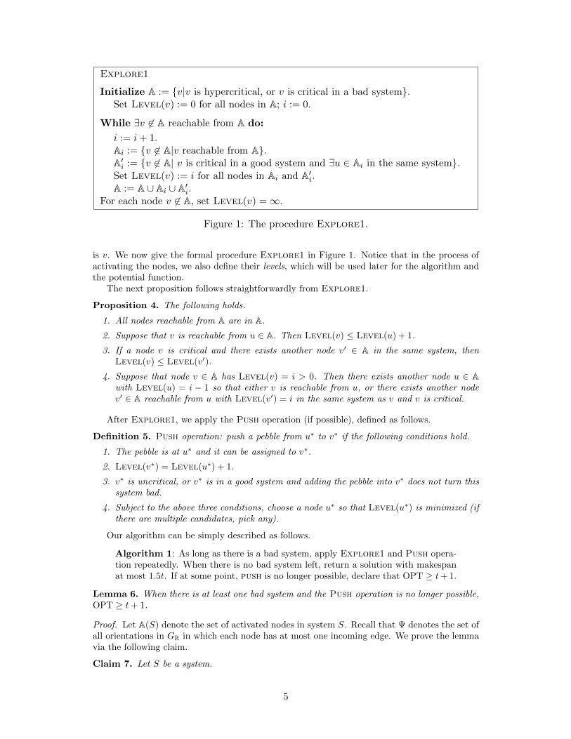
Explore1

Initialize A := {v|v is hypercritical, or v is critical in a bad system}.Set Level(v) := 0 for all nodes in A; i := 0.

While ∃v 6∈ A reachable from A do:

i := i+ 1.Ai := {v 6∈ A|v reachable from A}.A′i := {v 6∈ A| v is critical in a good system and ∃u ∈ Ai in the same system}.Set Level(v) := i for all nodes in Ai and A′i.A := A ∪ Ai ∪ A′i.

For each node v 6∈ A, set Level(v) =∞.

Figure 1: The procedure Explore1.

is v. We now give the formal procedure Explore1 in Figure 1. Notice that in the process ofactivating the nodes, we also define their levels, which will be used later for the algorithm andthe potential function.

The next proposition follows straightforwardly from Explore1.

Proposition 4. The following holds.

1. All nodes reachable from A are in A.

2. Suppose that v is reachable from u ∈ A. Then Level(v) ≤ Level(u) + 1.

3. If a node v is critical and there exists another node v′ ∈ A in the same system, thenLevel(v) ≤ Level(v′).

4. Suppose that node v ∈ A has Level(v) = i > 0. Then there exists another node u ∈ Awith Level(u) = i − 1 so that either v is reachable from u, or there exists another nodev′ ∈ A reachable from u with Level(v′) = i in the same system as v and v is critical.

After Explore1, we apply the Push operation (if possible), defined as follows.

Definition 5. Push operation: push a pebble from u∗ to v∗ if the following conditions hold.

1. The pebble is at u∗ and it can be assigned to v∗.

2. Level(v∗) = Level(u∗) + 1.

3. v∗ is uncritical, or v∗ is in a good system and adding the pebble into v∗ does not turn thissystem bad.

4. Subject to the above three conditions, choose a node u∗ so that Level(u∗) is minimized (ifthere are multiple candidates, pick any).

Our algorithm can be simply described as follows.

Algorithm 1: As long as there is a bad system, apply Explore1 and Push opera-tion repeatedly. When there is no bad system left, return a solution with makespanat most 1.5t. If at some point, push is no longer possible, declare that OPT ≥ t+ 1.

Lemma 6. When there is at least one bad system and the Push operation is no longer possible,OPT ≥ t+ 1.

Proof. Let A(S) denote the set of activated nodes in system S. Recall that Ψ denotes the set ofall orientations in GR in which each node has at most one incoming edge. We prove the lemmavia the following claim.

Claim 7. Let S be a system.

5

• Suppose that S is bad. Then

W · (minψ∈Ψ

number of rocks to A(S) according to ψ) +∑

v∈A(S)

pl(v) + dl(v) > |A(S)|t. (1)

• Suppose that S is good. Then

W ·(minψ∈Ψ

number of rocks to A(S) according to ψ)+∑

v∈A(S)

pl(v)+dl(v) > |A(S)|t−w. (2)

Observe that the term |A(S)|t is the maximum total weight that all nodes in A(S) canhandle if OPT ≤ t. As pebbles owned by nodes in A can only be assigned to the nodes inA, by the pigeonhole principle, in all orientations ψ ∈ Ψ, and all possible assignments of thepebbles, at least one bad system S has at least the same number of pebbles in A(S) as thecurrent assignment, or a good system S has at least one more pebble than it currently has inA(S). In both cases, we reach a contradiction.

Proof of Claim 7: First observe that in all orientations in Ψ, the nodes in A(S) have to receiveat least |A(S)| − 1 rocks. If S is a cycle, then the nodes in A(S) have to receive exactly |A(S)|rocks.

Next observe that none of the nodes in A(S) is uncritical, since otherwise, by Proposition 4.4and Definition 5.3, the Push operation would still be possible. By the same reasoning, if S is atree and A(S) 6= ∅, at least one node v ∈ A(S) is critical; furthermore, if |A(S)| = 1, this nodev satisfies dl(v) + pl(v) > 1.5t − w, as one more pebble would make v hypercritical. Similarly,if S is an isolated node v ∈ A, then dl(v) + pl(v) > 1.5t− w.

We now prove the claim by the following case analysis.

1. Suppose that S is a good system and A(S) 6= ∅. Then either S is a tree and A(S) containsexactly one critical (but not hypercritical) node, or S is an isolated node, or S is a cycleand has no critical node. In the first case, if |A(S)| ≥ 2, the LHS of (2) is at least

(1.5t−W + 1) + (|A(S)| − 1)(1.5t−W − w + 1) + (|A(S)| − 1)W =

|A(S)|t+ (|A(S)| − 2)(0.5t− w + 1) + t−W − w + 2 > |A(S)|t− w,

using the fact that 0.5t ≥ w, t ≥ W , and |A(S)| ≥ 2. If, on the other hand, |A(S)| = 1,then the LHS of (2) is strictly more than

1.5t− w ≥ t = |A(S)|t,

and the same also holds for the case when S is an isolated node. Finally, in the third case,the LHS of (2) is at least

|A(S)|(1.5t−W − w + 1) + |A(S)|W > |A(S)|t.

2. Suppose that A(S) contains at least two critical nodes, or that S is a cycle and A(S) hasat least one critical node. In both cases, S is a bad system. Furthermore, the LHS of (1)can be lower-bounded by the same calculation as in the previous case with an extra termof w.

3. Suppose that A(S) contains a hypercritical node. Then the system S is bad, and the LHSof (1) is at least

(1.5t+ 1) + (|A(S)| − 1)(1.5t−W − w + 1) + (|A(S)| − 1)W =

|A(S)|t+ (|A(S)| − 1)(0.5t− w + 1) + 0.5t+ 1 > |A(S)|t,

where the inequality holds because 0.5t ≥ w.

6

We argue that Algorithm 1 terminates in polynomial time by the aid of a potential function,defined as

Φ =∑v∈A

(|V | − Level(v)) · (number of pebbles at v).

Trivially, 0 ≤ Φ ≤ |V | · |P|. The next lemma implies that Φ is monotonically decreasing aftereach Push operation.

Lemma 8. For each node v ∈ V , let Level(v) and Level′(v) denote the levels before and aftera Push operation, respectively. Then Level′(v) ≥ Level(v).

Proof. We prove by contradiction. Suppose that there exist nodes x with Level′(x) < Level(x).Choose v to be one among them with minimum Level′(v). By the choice of v, and Definition 5.3,Level′(v) > 0 and v ∈ A after the Push operation. Thus, by Proposition 4.4, there exists anode u with Level′(u) = Level′(v)− 1, so that after Push,

• Case 1: v is reachable from u ∈ A, or

• Case 2: there exists another node v′ ∈ A reachable from u ∈ A with Level′(v′) =Level′(v) in the same system as v, and v is critical.

Notice that by the choice of v, in both cases, Level′(u) ≥ Level(u), and u ∈ A also beforethe Push operation. Let p be the pebble by which u reaches v (Case 1), or v′ (Case 2), afterPush. Before the Push operation, p was at some node u′ ∈ A (u′ may be u, or p is the pebblepushed: from u′ to u).

By Proposition 4.2, in Case 1, Level(v) ≤ Level(u′) + 1 (as v is reachable from u′ viap before Push), and Level(v′) ≤ Level(u′) + 1 in Case 2. Furthermore, if in Case 2 v wasalready critical before push, then Level(v) ≤ Level(v′) by Proposition 4.3 (note that v′ ∈ Aas it is reachable from u′ ∈ A). Hence, in both cases we would have

Level(v) ≤ Level(u′) + 1 ≤ Level(u) + 1 ≤ Level′(u) + 1 = Level′(v),

a contradiction. Note that the second inequality holds no matter u = u′ or not.Finally consider Case 2 where v was not critical before the Push operation. Then a pebble

p′ 6= p is pushed into v in the operation. Note that in this situation, v’s system is a tree andcontains no critical nodes before Push (since otherwise the operation would turn the systembad); in particular v′ is not critical. Furthermore, the presence of p in u implies that Level(v′) ≤Level(u) + 1 by Proposition 4.2, and that v′ ∈ A by Proposition 4.1. As v′ is not critical,Level(v′) > 0, and by Proposition 4.4 there exists a node u′′ with Level(u′′) = Level(v′)− 1so that u′′ can reach v′ by a pebble p′′ (u′′ may be u and p′′ may be p). As

Level(v′) ≤ Level(u) + 1 ≤ Level′(u) + 1 = Level′(v) < Level(v),

the Push operation should have pushed p′′ into v′ instead of p′ into v (see Definition 5.4), sinceu′′ and v′ satisfy all the first three conditions of Definition 5.

By Lemma 8 and the fact that a pebble is pushed to a node with higher level, the potential Φstrictly decreases after each Push operation, implying that Algorithm 1 finishes in polynomialtime.

Approximation Ratio: When t < 2W , we apply Algorithm 1. In the case of t ≥ 2W , weapply the algorithm of Gairing et al. [4], which either correctly reports that OPT ≥ t + 1, orreturns an assignment with makespan at most t+W − 1 < 1.5t.

Suppose that t is the smallest number for which an assignment is returned. Then OPT ≥ t,and our approximation ratio is bounded by 1.5t

OPT ≤ 1.5. We use a theorem to conclude thissection.

7

Theorem 9. With arbitrary dedicated loads on the machines, jobs of weight W that can beassigned to two machines, and jobs of weight w that can be assigned to any number of machines,we can find a 1.5 approximate solution in polynomial time.

In the appendix, we show that a slight modification of our algorithm yields an improved

approximation ratio of 1 +bW2 cW if W ≥ 2w.

4 The General Case

In this section, we describe the core algorithm for the case of arbitrary job weights. Thisalgorithm inherits some basic ideas from the previous section, but has several significantly newingredients—mainly due to the fact that the rocks now have different weights. Before formallypresenting the algorithm, let us build up intuition by looking at some examples.

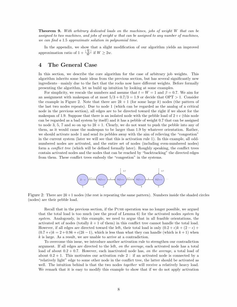
For simplicity, we rescale the numbers and assume that t = W = 1 and β = 0.7. We aim foran assignment with makespan of at most 5/3 + 0.7/3 = 1.9 or decide that OPT > 1. Considerthe example in Figure 2. Note that there are 2k + 1 (for some large k) nodes (the pattern ofthe last two nodes repeats). Due to node 1 (which can be regarded as the analog of a criticalnode in the previous section), all edges are to be directed toward the right if we shoot for themakespan of 1.9. Suppose that there is an isolated node with the pebble load of 2 + ε (this nodecan be regarded as a bad system by itself) and it has a pebble of weight 0.7 that can be assignedto node 3, 5, 7 and so on up to 2k + 1. Clearly, we do not want to push the pebble into any ofthem, as it would cause the makespan to be larger than 1.9 by whatever orientation. Rather,we should activate node 1 and send its pebbles away with the aim of relieving the “congestion”in the current system (later we will see that this is activation rule 1). In this example, all odd-numbered nodes are activated, and the entire set of nodes (including even-numbered nodes)form a conflict tree (which will be defined formally later). Roughly speaking, the conflict treescontain activated nodes and the nodes that can be reached by “backtracking” the directed edgesfrom them. These conflict trees embody the “congestion” in the systems.

2− ǫ0.7 + ǫ

0.2 + ǫ 0.2 + ǫ0.2 + ǫ 0.2 + ǫ0.7 + ǫ 1

1 2 3 4 5

0.7 0.7

1 · · ·

Figure 2: There are 2k+1 nodes (the rest is repeating the same pattern). Numbers inside the shaded circles(nodes) are their pebble load.

Recall that in the previous section, if the Push operation was no longer possible, we arguedthat the total load is too much (see the proof of Lemma 6) for the activated nodes system bysystem. Analogously, in this example, we need to argue that in all feasible orientations, theactivated set of nodes (totally k + 1 of them) in this conflict tree cannot handle the total load.However, if all edges are directed toward the left, their total load is only (0.2 + ε)k + (2− ε) +(0.7 + ε)k = 2 + 0.9k+ ε(2k− 1), which is less than what they can handle (which is k+ 1) whenk is large. As a result, we are unable to arrive at a contradiction.

To overcome this issue, we introduce another activation rule to strengthen our contradictionargument. If all edges are directed to the left, on the average, each activated node has a totalload of about 0.2 + 0.7. However, each inactivated node has, on the average, a total load ofabout 0.2 + 1. This motivates our activation rule 2 : if an activated node is connected by a“relatively light” edge to some other node in the conflict tree, the latter should be activated aswell. The intuition behind is that the two nodes together will receive a relatively heavy load.We remark that it is easy to modify this example to show that if we do not apply activation

8

0.70.7

11

11

0.7 + ǫ0.7 + ǫ

0.2 + ǫ 0.2 + ǫ

0.3 + ǫ 1 + ǫ

0.2 0.2

1 1

0.7

1

2

3

4

1′

2′

3′

4′

Figure 3: A naive Push will oscillate the pebblebetween nodes 4 and 4′.

0.70.7

11

11

0.7 + ǫ0.7 + ǫ

0.2 + ǫ 0.2 + ǫ

0.3 + ǫ 1 + ǫ

0.2 0.2

1 1

0.7

1

2

3

4

1′

2′

3′

4′

Figure 4: A fake orientation from node 2 to 3causes node 4 to have an incoming edge, thus in-forming node 4′ not to push the pebble.

rule 2, then we cannot hope for a 2− δ approximation for any small δ > 0. 2

Next consider the example in Figure 3. Here nodes 2, 2′, and 4′ can be regarded as thecritical nodes, and {1, 2}, {1′, 2′, 3′, 4′} are the two conflict trees. Both nodes 1 and 1′ can bereached by an isolated node with heavy load (the bad system) with a pebble of weight 0.7.Suppose further that node 4′ can reach node 4 by another pebble of weight 0.7. It is easy to seethat a naive Push definition will simply “oscillate” the pebble between nodes 4 and 4′, causingthe algorithm to cycle.

Intuitively, it is not right to push the pebble from 4′ into 4, as it causes the conflict treeon the left system to become bigger. Our principle of pushing a pebble should be to relievethe congestion in one system, while not worsening the congestion in another. To cope with thisproblematic case, we use fake orientations, i.e., we direct edges away from a conflict tree, asshown in Figure 4. Node 2 directs the edge toward node 3, which in turn causes the next edgeto be directed toward node 4. With the new incoming edge, node 4 now has a total load of1 + 0.3 + ε to handle, and the pebble thus will not be pushed from node 4′ to node 4.

4.1 Formal description of the algorithm

We inherit some terminology from the previous section. We say that v is reachable from u ifa pebble in u can be assigned to v, and that v is reachable from A if v is reachable from anynode u ∈ A. Each tree, cycle, isolated node in GR is a system. Note that there is exactly oneedge between two adjacent nodes in GR (see Proposition 1). For ease of presentation, we usethe short hand vu to refer to the edge {v, u} in GR and wvu is its weight.

The orientation of the edges in GR will be decided dynamically. If uv is directed toward v,we call v a father of u, and u a child of v. We write rl(v) to denote total weight of the rocksthat are (currently) oriented towards v (and pl(v) still denotes the total weight of the pebblesat v). An edge that is currently un-oriented is neutral. In the beginning, all edges in GR areneutral.

2Looking at this particular example, one is tempted to use the idea of activating all nodes in the conflict tree.However, such an activation rule will not work. Consider the following example: There are k + 2 nodes forming apath, and the k + 1 edges connecting them all have weight 0.95 + ε. The first node has a pebble load of 1 and thus“forces” an orientation of the entire path (for a makespan of at most 1.9). The next k nodes have a pebble load of0, and the last node has a pebble load of 0.25 and is reachable from a bad system via a pebble of weight 0.7. Theconflict tree is the entire path, and activating all nodes leads to a total load of (k + 1) · (0.95 + ε) + 1 + 0.25, whichis less than k + 2 for large k.

9

A set C of nodes, called the conflict trees, will be collected in the course of the algorithm.Let D(v) := {u ∈ C : u is child of v} and F(v) := {u ∈ C : u is father of v} for any v ∈ C. Anode v ∈ C is a leaf if D(v) = ∅, and a root if F(v) = ∅. Furthermore, a node v is overloaded ifdl(v) + pl(v) + rl(v) > (5/3 + β/3)t, and a node v ∈ C is critical if there exists u ∈ F(v) suchthat dl(v) + pl(v) + wvu > (5/3 + β/3)t. In other words, a node in the conflict trees is criticalif it has enough load by itself (without considering incoming rocks) to “force” an incident edgeto be directed toward a father in the conflict trees.

Initially, the pebbles are arbitrarily assigned to the nodes. The orientation of a subset of theedges in GR is determined by the procedure Forced Orientations in Figure 5.

Forced Orientations

While ∃ neutral edge vu in GR, s.t. dl(v) + pl(v) + rl(v) + wvu > (5/3 + β/3)t:

Direct vu towards u; Marked := {u}.While ∃ neutral edge v′u′ in GR, s.t. dl(v′) + pl(v′) + rl(v′) +wv′u′ > (5/3 + β/3)t

and v′ ∈Marked:

Direct v′u′ towards u′; Marked := Marked ∪ {u′}.

Figure 5: The procedure Forced Orientations.

Intuitively, the procedure first finds a “source node” v, whose dedicated, pebble, and rockload is so high that it “forces” an incident edge vu to be oriented away from v. The orientationof this edge then propagates through the graph, i.e. edge-orientations induced by the directionof vu are established. Then the next “source” is found, and so on. To simplify our proofs, weassume that ties are broken according to a fixed total order if several pairs (v, u) satisfy theconditions of the while-loops.

Lemma 10. Suppose that all edges in GR are neutral and Forced Orientations is called.Then after the procedure, every overloaded node v has at most one incoming edge.

Proof. We start with the following observation. Let vu be the first edge directed in someiteration of the outer while-loop. If v′u′ is directed in the same iteration of the outer while-loop,then there exists a directed path starting with the edge uv and ending with the edge v′u′.

Now suppose that some node w is overloaded after the procedure and has more than oneincoming edge. Let wx and wy be the last two edges directed toward w, and note that both,wx and wy, become directed in the same iteration of the outer while-loop (because as soon asone of the two is directed toward w, the other edge satisfies the conditions of the inner while-loop). Hence, there are two different directed paths towards w (with final edges wx and wy,respectively), both of which start with the first edge that becomes directed in this iteration ofthe outer while-loop. This implies that w’s system contains a cycle and a node of degree at least3, a contradiction.

Clearly, if after the procedure Forced Orientations a node v still has a neutral incidentedge vu, then dl(v) + pl(v) + rl(v) +wvu ≤ (5/3 +β/3)t. Now suppose that after the procedure,none of the nodes is overloaded. Then orienting the neutral edges in each system in such a waythat every node has at most one more incoming edge gives us a solution with makespan at most(5/3+β/3)t. So assume the procedure ends with a non-empty set of overloaded nodes. We thenapply the procedure Explore2 in Figure 6.

Let us elaborate the procedure. In each round, we perform the following three tasks.

1. Add those nodes reachable from the nodes in Ai−1 into Ai in case of i > 1; or the overloadednodes into Ai in case of i = 0. These nodes will be referred to as Type A nodes.

2. In the sub-procedure Constructing conflict trees, nodes not in the conflicts trees and havinga directed path to those Type A nodes in Ai are continuously added into the conflict trees

10

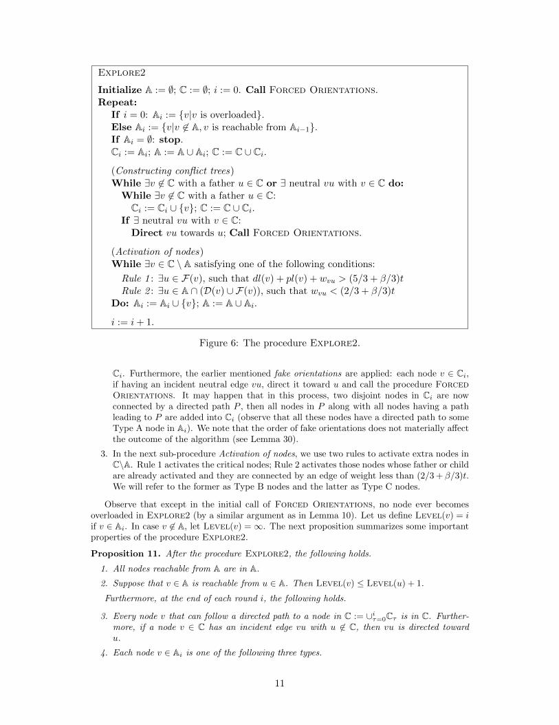
Explore2

Initialize A := ∅; C := ∅; i := 0. Call Forced Orientations.Repeat:

If i = 0: Ai := {v|v is overloaded}.Else Ai := {v|v 6∈ A, v is reachable from Ai−1}.If Ai = ∅: stop.Ci := Ai; A := A ∪ Ai; C := C ∪ Ci.

(Constructing conflict trees)While ∃v 6∈ C with a father u ∈ C or ∃ neutral vu with v ∈ C do:

While ∃v 6∈ C with a father u ∈ C:Ci := Ci ∪ {v}; C := C ∪ Ci.

If ∃ neutral vu with v ∈ C:Direct vu towards u; Call Forced Orientations.

(Activation of nodes)While ∃v ∈ C \ A satisfying one of the following conditions:

Rule 1 : ∃u ∈ F(v), such that dl(v) + pl(v) + wvu > (5/3 + β/3)tRule 2 : ∃u ∈ A ∩ (D(v) ∪ F(v)), such that wvu < (2/3 + β/3)t

Do: Ai := Ai ∪ {v}; A := A ∪ Ai.

i := i+ 1.

Figure 6: The procedure Explore2.

Ci. Furthermore, the earlier mentioned fake orientations are applied: each node v ∈ Ci,if having an incident neutral edge vu, direct it toward u and call the procedure ForcedOrientations. It may happen that in this process, two disjoint nodes in Ci are nowconnected by a directed path P , then all nodes in P along with all nodes having a pathleading to P are added into Ci (observe that all these nodes have a directed path to someType A node in Ai). We note that the order of fake orientations does not materially affectthe outcome of the algorithm (see Lemma 30).

3. In the next sub-procedure Activation of nodes, we use two rules to activate extra nodes inC\A. Rule 1 activates the critical nodes; Rule 2 activates those nodes whose father or childare already activated and they are connected by an edge of weight less than (2/3 + β/3)t.We will refer to the former as Type B nodes and the latter as Type C nodes.

Observe that except in the initial call of Forced Orientations, no node ever becomesoverloaded in Explore2 (by a similar argument as in Lemma 10). Let us define Level(v) = iif v ∈ Ai. In case v 6∈ A, let Level(v) =∞. The next proposition summarizes some importantproperties of the procedure Explore2.

Proposition 11. After the procedure Explore2, the following holds.

1. All nodes reachable from A are in A.

2. Suppose that v ∈ A is reachable from u ∈ A. Then Level(v) ≤ Level(u) + 1.

Furthermore, at the end of each round i, the following holds.

3. Every node v that can follow a directed path to a node in C := ∪iτ=0Cτ is in C. Further-more, if a node v ∈ C has an incident edge vu with u 6∈ C, then vu is directed towardu.

4. Each node v ∈ Ai is one of the following three types.

11

(a) Type A: there exists another node u ∈ Ai−1 so that v is reachable from u, or v isoverloaded and is part of A0.

(b) Type B: v is activated via Rule 1 (hence v is critical)3, and there exists a directedpath from v to u ∈ Ai of Type A.

(c) Type C: v is activated via Rule 2, and there exists an adjacent node u ∈ ∪iτ=0Aτ sothat wvu < (2/3 + β/3)t and u ∈ D(v) ∪ F(v).

After the procedure Explore2, we apply the Push operation (if possible), defined as follows.

Definition 12. Push operation: push a pebble from u∗ to v∗ if the following conditions hold(if there are multiple candidates, pick any).

1. The pebble is at u∗ and it can be assigned to v∗.

2. Level(v∗) = Level(u∗) + 1.

3. dl(v∗) + pl(v∗) + rl(v∗) ≤ (5/3− 2/3 · β)t.

4. D(v∗) = ∅, or dl(v∗) + pl(v∗) + wv∗u ≤ (5/3− 2/3 · β)t for all u ∈ F(v).

Definition 12(3) is meant to make sure that v∗ does not become overloaded after receivinga new pebble (whose weight can be as heavy as βt). Definition 12(4) says either v∗ is a leaf, oradding a pebble with weight as heavy as βt does not cause v∗ to become critical.

Algorithm 2: Apply Explore2. If it ends with A0 = ∅, return a solution withmakespan at most (5/3 + β/3)t. Otherwise, apply Push. If push is impossible,declare that OPT ≥ t+ 1. Un-orient all edges in GR and repeat this process.

Lemma 13. When there is at least one overloaded node and the Push operation is no longerpossible, OPT ≥ t+ 1.

Lemma 14. For each node v ∈ V , let Level(v) and Level′(v) denote the levels before andafter a Push operation, respectively. Then Level′(v) ≥ Level(v).

The preceding two lemma are proven in sections 4.2 and 4.3, respectively. We again use thepotential function

Φ =∑v∈A

(|V | − Level(v)) · (number of pebbles at v)

to argue the polynomial running time of Algorithm 2. Trivially, 0 ≤ Φ ≤ |V | · |P|. Fur-thermore, by Lemma 14 and the fact that a pebble is pushed to a node with higher level, thepotential Φ strictly decreases after each Push operation. This implies that Algorithm 2 finishesin polynomial time.

We can therefore conclude:

Theorem 15. Let β ∈ [4/7, 1). With arbitrary dedicated loads on the machines, if jobs ofweight greater than βW can be assigned to only two machines, and jobs of weight at most βWcan be assigned to any number of machines, we can find a 5/3 + β/3 approximate solution inpolynomial time.

4.2 Proof Of Lemma 13

Our goal is to show that in any feasible solution, the activated nodes A must handle a total loadof more than |A|t, which implies that OPT ≥ t+1. For the proof, we focus on a single componentK of GR[C], the subgraph of GR induced by the conflict trees C, and a fixed orientation ψ ∈ Ψ.Let ψ(v) denote the total weight of the rocks assigned to any v ∈ A by ψ (note that 0 ≤ ψ(v) ≤ t),and let A(K) denote the set of activated nodes in K. We will show that

3For simplicity, if a node can be activated by both Rule 1 and Rule 2, we assume it is activated by Rule 1.

12

∑v∈A(K)

pl(v) + dl(v) + ψ(v) > |A(K)|t (3)

if A(K) 6= ∅. The lemma then follows by summing over all components of GR[C], and notingthat the pebbles on the nodes in A can only be assigned to the nodes in A (Proposition 11(1)).

If K consists only of a single activated node v, then (3) clearly holds, as pl(v) + dl(v) >(5/3− 2/3 · β)t ≥ t (since v is a Type A node and push is no longer possible). In the following,we will assume that F(v) ∪ D(v) 6= ∅ for all v ∈ A(K).

Definition 16. For every non-leaf v ∈ A(K), fix some node d(v) ∈ D(v), such that wvd(v) =maxu∈D(v) wvu.

Definition 17. For every non-root v ∈ A(K), fix some node f(v) ∈ F(v), such that wvf(v) =maxu∈F(v) wvu.

Definition 18. For every node v ∈ A(K) that is neither a root nor a leaf, fix some noden(v) ∈ D(v) ∪ F(v), such that wvn(v) = maxu∈D(v)∪F(v) wvu.

Definition 19. For every node v ∈ A(K) that was activated using Rule 2 in the final executionof Explore2, fix some node a(v) ∈ A(K) ∩ (D(v) ∪ F(v)) with wva(v) < (2/3 + β/3)t, suchthat a(v) has been activated before v.

We classify the nodes v ∈ A(K) that are neither a root nor a leaf, into the following threetypes.

Type 1: |D(v)| > 1.

Type 2: |D(v)| = 1 and v was activated via Rule 2 (i.e., as a Type C node).

Type 3: |D(v)| = 1 and v was not activated via Rule 2 (i.e. as a Type A or Type B node).

In the following, we summarize the inequalities that we use for the different types of nodes,in order to prove (3). We refer to them as the load-inequalities.

Claim 20. For every leaf v ∈ A(K), pl(v) + dl(v) > (5/3 + β/3)t− wvf(v).

Proof. If v ∈ Ai is activated as a Type A node, then it is either overloaded or is reachable from anode u ∈ Ai−1. In both cases, since push is no longer possible, pl(v)+dl(v)+rl(v) > (5/3−2/3 ·β)t. The claim follows as rl(v) = 0 and wvf(v) > βt. If v is not activated as a Type A node, thenv first becomes part of C and then becomes activated via Rule 1 or Rule 2. In this case, at themoment v becomes part of C, it must have a father u ∈ C. The edge vu becomes oriented towardsu only when Forced Orientations is called and dl(v) + pl(v) + rl(v) + wvu > (5/3 + β/3)t.The claim follows again as rl(v) = 0 and wvf(v) ≥ wvu.

Claim 21. For every root v ∈ A(K) with |D(v)| = 1, pl(v) + dl(v) > (5/3− 2/3 · β)t−wvd(v).

Proof. As v ∈ Ai has no father in C, it must either be overloaded or reachable from an activatednode u ∈ Ai−1. In both cases, pl(v) + dl(v) + rl(v) > (5/3− 2/3 · β)t, since the Push operationis no longer possible. The claim follows as |D(v)| = 1 implies wvd(v) ≥ rl(v).

Claim 22. For every root v ∈ A(K) with |D(v)| > 1, pl(v) + dl(v) ≥ 0.

Proof. Trivially true.

Claim 23. For every Type 1 node v ∈ A(K), pl(v) + dl(v) ≥ 0.

Proof. Trivially true.

Claim 24. For every Type 2 node v ∈ A(K), pl(v) + dl(v) > (5/3 + β/3)t− wvf(v) − wvd(v).

13

Proof. As v is activated using Rule 2, it first becomes part of C without being activated. Forthis to happen, it must have a father u ∈ C. The edge vu becomes oriented towards u onlywhen Forced Orientations is called and dl(v) + pl(v) + rl(v) + wvu > (5/3 + β/3)t. Theclaim follows as wvd(v) ≥ rl(v) (since |D(v)| = 1) and wvf(v) ≥ wvu.

Claim 25. For every Type 3 node v ∈ A(K), pl(v) + dl(v) > (5/3− 2/3 · β)t− wvn(v).

Proof. If v is overloaded, the claim directly follows from the fact that wvn(v) ≥ rl(v). Further-more, if v ∈ Ai is reachable from an activated node u ∈ Ai−1, then the claim follows from thedefinition of n(v) and the fact that either the third or the fourth condition of push must beviolated. The only other possibility for v to be activated is via Rule 1, which together with thedefinition of n(v) implies our claim.

To prove (3), we look at each node v ∈ A(K) separately and calculate how much it contributesto the balance under some simplifying assumptions. In the end, we will see that the nodes inA(K) have enough load to compensate for the assumptions we made.

Let EA(K) denote the edges of K that are incident with the nodes A(K), i.e. EA(K) := {vu ∈R : u ∈ A(K), v ∈ D(u) ∪ F(u)}. We say that an edge vu ∈ EA(K) is covered if wvu appearson the right-hand side of u’s and/or v’s load-inequality. For example, if v is a leaf, then vf(v)is covered. Every edge in EA(K) that is not covered is called uncovered. Finally, we say thatan edge vu ∈ EA(K) is doubly covered if wvu appears on the right-hand side of both u’s and v’sload-inequality.

We distinguish two cases.

4.2.1 Case 1: K is a tree.

Claim 26. K contains 1+∑v∈K:F(v)6=∅(|F(v)|−1) many roots, and 1+

∑v∈K:D(v)6=∅(|D(v)|−1)

many leaves. Furthermore, every root and leaf in K is activated.

Proof. The first part simply follows from the degree sum formula for directed graphs and thefact that K is a tree. For the second part, observe that any node v ∈ C that is not activatedas Type A node, must have had a father u ∈ C already before it got added into C itself. Thisproves that every root in K is activated (as a Type A node).

If a leaf v ∈ C is not activated as Type A node, then its incident edge vu with u ∈ C isoriented toward u only when Forced Orientations is called and dl(v) +pl(v) + rl(v) +wvu >(5/3 + β/3)t. As v ∈ C ends up a leaf, rl(v) = 0, and Rule 1 would have applied to v. So everyleaf in K is activated.

In our calculations, we will assume that every covered edge vu ∈ EA(K) has weight wvu = t,and that ψ(v) = t for all v ∈ A(K). With these assumptions, we will show that∑

v∈A(K)

pl(v) + dl(v) + ψ(v) > |A(K)|t

− |{doubly covered vu ∈ EA(K) : wvu < (2/3 + β/3)t}| · (1/3− β/3)t

+ |{uncovered vu ∈ EA(K)}| · (t− wvu)

+ t.

(4)

Let us consider the error caused by these two assumptions when we lower-bound the term∑v∈A(K) pl(v) + dl(v) + ψ(v), and in doing so, we will show why (4) implies (3).

Consider an edge vu ∈ EA(K) that ψ assigns to a node in A(K), say v. Consider threepossibilities.

• If vu is covered, then wvu appears on the LHS of (3) as a negative term after we plug inthe load-inequalities, and the two terms ψ(v) and wvu cancel each other. Hence, in thiscase, we make no error by assuming both terms to be equal to t.

14

• If vu is doubly covered and wvu < (2/3 + β/3)t, our assumptions underestimate the load∑v∈A(K) pl(v) + dl(v) + ψ(v) by more than (1/3− β/3)t.

• If vu is uncovered, then we overestimate ψ(v) by at most t− wvu.

Finally, we note that ψ must assign an edge from EA(K) to every node in A(K) exceptfor possibly one. For this special node v∗ that does not receive an edge from EA(K) underψ, we overestimate ψ(v∗) by at most t. In conclusion, when we remove our assumptions,∑v∈A(K) pl(v) + dl(v) + ψ(v) increases by more than (1/3 − β/3)t per doubly covered edge

vu ∈ EA(K) with wvu < (2/3 + β/3)t, and decreases by at most t − wvu per uncovered edgevu ∈ EA(K), plus possibly another t for the special node v∗. Hence, if we prove inequality (4)under the aforementioned assumptions, (3) must hold after we remove the assumptions, andLemma 13 would follow.

We now turn to proving (4) when every covered edge vu ∈ EA(K) has weight wvu = t, andψ(v) = t for all v ∈ A(K). To this end, we consider the value pl(v) + dl(v) +ψ(v) as a budget ofnode v. Furthermore, we also assign budgets to edges vu ∈ EA(K) that are doubly covered andhave weight wvu < (2/3 + β/3)t. Each of them gets a budget of (1/3− β/3)t. Other remainingedges of EA(K) have budget 0.

By redistributing budgets between nodes and edges, we will ensure that eventually

(i) every node in A(K) has a budget of at least t,

(ii) there exists a leaf in A(K) with budget strictly greater than t+ (2/3 + β/3)t,

(iii) there exists a root in A(K) with budget at least t+ (2/3− 2/3 · β)t,

(iv) every uncovered edge vu ∈ EA(K) has a budget of at least t− wvu, and

(v) no edge in EA(K) has negative budget.

This would complete the proof.We start with the leaf nodes. If v ∈ A(K) is a leaf, then (using Claim 20) it has a budget of

more than (5/3 + β/3)t− wvf(v) + ψ(v) = (5/3 + β/3)t. Using Claim 26, we can therefore add(|D(u)| − 1) · (2/3 + β/3)t to the budget of every non-leaf u ∈ A(K), such that (i) and (ii) arestill satisfied for all leaves.

Next we consider the roots. If v ∈ A(K) is a root and |D(v)| = 1, then (using Claim 21) it hasa budget of more than (5/3−2/3·β)t. If v ∈ A(K) is a root and |D(v)| > 1, then (using Claim 22and the load added in the previous step) it has a budget of at least t+(|D(v)|−1) · (2/3+β/3)t.In the latter case, we transfer (2/3 − 2/3 · β)t to the budget of every edge in EA(K) that isincident with v. The budget of v thereby remains at least t+(|D(v)|−1) · (2/3+β/3)t−|D(v)| ·(2/3− 2/3 · β)t = (1/3− β/3)t+ |D(v)| · βt ≥ (5/3− 2/3 · β)t, where the last inequality followsfrom |D(v)| ≥ 2 and β ≥ 4/7. Using Claim 26, we can thus add (|F(u)| − 1) · (2/3− 2/3 · β)t tothe budget of every non-root u ∈ A(K), such that (i) and (iii) are satisfied for all roots.

Before we move on to Type 1, 2, and 3 nodes, we take one step back and visit the leavesagain, as their budget has increased again through the latest redistribution of load. Namely,every leaf v ∈ A(K) got an additional load of (|F(v)| − 1) · (2/3− 2/3 · β)t, which we now useto add (2/3 − 2/3 · β)t to the budget of every edge in EA(K) that is incident with v, except tovf(v) (which is surely covered). After this, (ii) and (iii) are satisfied, (i) holds for every rootand every leaf, and every uncovered edge vu ∈ EA(K) that is incident with a root or a leaf hasa budget of at least (2/3− 2/3 · β)t.

Let us now consider the nodes of Type 1. Such a node v (using Claim 23 and the loadadded in previous steps) has a budget of at least t + (|D(v)| − 1) · (2/3 + β/3)t + (|F(v)| −1) · (2/3 − 2/3 · β)t. We transfer (2/3 − 2/3 · β)t to the budget of every edge in EA(K) that isincident with v. Since there are |D(v)| + |F(v)| such edges, the budget at v remains at leastt+(|D(v)|−1) · (2/3+β/3)t− (|D(v)|+1) · (2/3−2/3 ·β)t = (|D(v)|+1)βt− (1/3+2/3 ·β)t ≥ t,as |D(v)| ≥ 2 and β ≥ 4/7.

Next we consider the nodes of Type 2. Such a node v (using Claim 24 and the load addedin previous steps) has a budget of more than (2/3 + β/3)t+ (|F(v)| − 1) · (2/3− 2/3 · β)t. We

15

transfer (2/3− 2/3 · β)t to the budget of every edge in EA(K) that is incident with v, except tovf(v) and vd(v) (which are surely covered). Since there are |F(v)| − 1 such edges, the resultingbudget at v is still more than (2/3 + β/3)t. We now reduce the budget of the edge va(v) by(1/3 − β/3)t and add this load to v’s budget, which is then more than t. We will show laterthat this last step (reducing the budget of va(v)) does not cause a violation of (v).

Finally, we consider the nodes of Type 3. Such a node v (using Claim 25 and the load addedin previous steps) has a budget of more than (5/3 − 2/3 · β)t + (|F(v)| − 1) · (2/3 − 2/3 · β)t.We transfer (2/3− 2/3 ·β)t to the budget of every edge in EA(K) that is incident with v, exceptto vn(v) (which is surely covered). Since there are |F(v)| such edges, the resulting budget at vis still more than t.

After the above redistributions of load, (i), (ii), and (iii) are satisfied. Furthermore, supposethat some edge vu ∈ EA(K) is uncovered and has weight wvu ≥ (2/3+β/3)t. Then at least once,we have added (2/3 − 2/3 · β)t to the budget of this edge, and we never reduced it. Thereforeit has a budget of at least (2/3 − 2/3 · β)t ≥ (1/3 − β/3)t ≥ t − wvu, and (iv) holds for thisedge. If, on the other hand, an uncovered edge vu ∈ EA(K) has weight wvu < (2/3 + β/3)t,then both u and v are in A(K) (due to activation rule 2), and (2/3− 2/3 · β)t was added twiceto the budget of vu. Furthermore, if this budget got reduced at some point, then at most once(u = a(v) and v = a(u) cannot happen simultaneously). The final budget of vu is thus at least2 · (2/3− 2/3 · β)t− (1/3− β/3)t = t− βt > t−wvu. Hence, for such an edge the assertion (iv)also holds.

Finally, for (v), observe that the only point where we reduce the budget of a covered edgevu ∈ EA(K) and add it to v’s budget, is when v is of Type 2, wvu < (2/3 + β/3)t, and u = a(v).Furthermore, both u and v have to be in A(K) (due to activation rule 2). In this case, thebudget of vu is reduced exactly once, by a value of (1/3−β/3)t. If vu is doubly covered, then ithad an initial budget of (1/3− β/3)t, and its budget therefore remains non-negative. If, on theother hand, vu is covered but not doubly covered, then at some point its budget was increased by(2/3−2/3·β)t. Hence, the final budget is at least (2/3−2/3·β)t−(1/3−β/3)t = (1/3−β/3)t ≥ 0.This concludes the proof.

4.2.2 Case 2: K is a cycle.

Claim 27. K contains∑v∈K:F(v)6=∅(|F(v)|−1) many roots, and

∑v∈K:D(v) 6=∅(|D(v)|−1) many

leaves. Furthermore, every root and leaf in K is activated.

Proof. The first part simply follows from the degree sum formula for directed graphs and thefact that K is a cycle. The second part is analogous to Claim 26.

We will again assume that every covered edge vu ∈ EA(K) has weight wvu = t, and thatψ(v) = t for all v ∈ A(K). With these assumptions, we will show that∑

v∈A(K)

pl(v) + dl(v) + ψ(v) > |A(K)|t

− |{doubly covered vu ∈ EA(K) : wvu < (2/3 + β/3)t}| · (1/3− β/3)t

+ |{uncovered vu ∈ EA(K)}| · (t− wvu).

(5)

By the same arguments as in Case 1, the error caused by the above two assumptions whenwe lower-bound the term

∑v∈A(K) pl(v) + dl(v) + ψ(v) is:

• we underestimate the term by more than (1/3−β/3)t per doubly covered edge vu ∈ EA(K)

with wvu < (2/3 + β/3)t,

• we overestimate the term by at most t− wvu per uncovered edge vu ∈ EA(K).

Note that, since K is a cycle, ψ must assign an edge from EA(K) to every node in A(K), andthus there is no special node v∗ as in Case 1. Hence, if we prove inequality (5) under theaforementioned assumptions, (3) must hold after we remove the assumptions, and Lemma 13would follow.

16

We now prove (5) when every covered edge vu ∈ EA(K) has weight wvu = t, and ψ(v) = tfor all v ∈ A(K). Again, we consider the value pl(v) + dl(v) + ψ(v) as a budget of node v.Furthermore, we also assign budgets to edges vu ∈ EA(K) that are doubly covered and haveweight wvu < (2/3 +β/3)t. Each of them gets a budget of (1/3−β/3)t. Other remaining edgesof EA(K) have budget 0.

By redistributing budgets between nodes and edges, we will ensure that eventually

(i) every node in A(K) has a budget of at least t,

(ii) at least one node in A(K) has a budget strictly greater than t,

(iii) every uncovered edge vu ∈ EA(K) has a budget of at least t− wvu, and

(iv) no edge in EA(K) has negative budget.

This would complete the proof.We start with the leaf nodes. If v ∈ A(K) is a leaf, then (using Claim 20) it has a budget

of more than (5/3 + β/3)t − wvf(v) + ψ(v) = (5/3 + β/3)t. Using Claim 27, we can thereforeadd (|D(u)| − 1) · (2/3 + β/3)t to the budget of every non-leaf u ∈ A(K), such that (i) is stillsatisfied for all leaves.

Next we consider the roots. If v ∈ A(K) is a root and |D(v)| = 1, then (using Claim 21) it hasa budget of more than (5/3−2/3·β)t. If v ∈ A(K) is a root and |D(v)| > 1, then (using Claim 22and the load added in the previous step) it has a budget of at least t+(|D(v)|−1) · (2/3+β/3)t.In the latter case, we transfer (2/3 − 2/3 · β)t to the budget of every edge in EA(K) that isincident with v. The budget of v thereby remains at least t+(|D(v)|−1) · (2/3+β/3)t−|D(v)| ·(2/3− 2/3 · β)t = (1/3− β/3)t+ |D(v)| · βt ≥ (5/3− 2/3 · β)t, where the last inequality followsfrom |D(v)| ≥ 2 and β ≥ 4/7. Using Claim 27, we can thus add (|F(u)| − 1) · (2/3− 2/3 · β)t tothe budget of every non-root u ∈ A(K), such that (i) is satisfied for all roots.

Before we move on to Type 1, 2, and 3 nodes, we take one step back and visit the leavesagain, as their budget has increased again through the latest redistribution of load. Namely,every leaf v ∈ A(K) got an additional load of (|F(v)| − 1) · (2/3− 2/3 ·β)t, which we now use toadd (2/3−2/3 ·β)t to the budget of every edge in EA(K) that is incident with v, except to vf(v)(which is surely covered). After this, (i) holds for every root and every leaf, and every uncoverededge vu ∈ EA(K) that is incident with a root or a leaf has a budget of at least (2/3− 2/3 · β)t.

As K is a cycle, there cannot be a node of Type 1, since every v ∈ A(K) with |D(v)| > 1 isa root.

Let us now consider the nodes of Type 2. Such a node v (using Claim 24 and the load addedin previous steps) has a budget of more than (2/3 + β/3)t+ (|F(v)| − 1) · (2/3− 2/3 · β)t. Wetransfer (2/3− 2/3 · β)t to the budget of every edge in EA(K) that is incident with v, except tovf(v) and vd(v) (which are surely covered). Since there are |F(v)| − 1 such edges, the resultingbudget at v is still more than (2/3 + β/3)t. We now reduce the budget of the edge va(v) by(1/3 − β/3)t and add this load to v’s budget, which is then more than t. We will show laterthat this last step (reducing the budget of va(v)) does not cause a violation of (iv).

Finally, we consider the nodes of Type 3. Such a node v (using Claim 25 and the load addedin previous steps) has a budget of more than (5/3 − 2/3 · β)t + (|F(v)| − 1) · (2/3 − 2/3 · β)t.We transfer (2/3− 2/3 ·β)t to the budget of every edge in EA(K) that is incident with v, exceptto vn(v) (which is surely covered). Since there are |F(v)| such edges, the resulting budget at vis still more than t.

After the above redistributions of load, (i) is satisfied. Furthermore, (ii) holds as at leastone node must be of Type 2, Type 3, or a leaf, and for all these cases the load-inequality is astrict inequality. Finally, the proof of (iii) and (iv) is exactly analogous to the proof of (iv) and(v) in Case 1.

4.3 Proof of Lemma 14

In the following, let E(V ′) denote the set of edges both of whose endpoints are in V ′ and δ(V ′)the set of edges exactly one of whose endpoints is in V ′, for each V ′ ⊆ V .

17

We prove the lemma by the following two steps.

Step 1: We create a clone of the pebble that is pushed from u∗ to v∗ and put this cloned pebbleat v∗ (by cloning, we mean the new pebble has the same weight and the same set of machines itcan be assigned to) and keep the old one at u∗. We apply Explore2 to this new instance andargue that the outcome is “essentially the same” as if the cloned pebble were not there. Moreprecisely, we show

Lemma 28. Suppose that Explore2 is applied to the original instance ( before Push) and

the new instance with the cloned pebble at v∗. Then at the end of each round i, Ai = A†i and

Ci = C†i , where Ai, A†i are the activated sets in the original and the new instances respectively,

and Ci and C†i are the conflict trees in the original and the new instances respectively.

Step 2: We then remove the original pebble at u∗ but keep the clone at v∗ (the same as theoriginal instance after Push). Reapplying Explore2, we then show that in each round, the setof activated nodes and the conflict trees cannot enlarge. To be precise, we show4

Lemma 29. Suppose that Explore2 is applied to the new instance with the cloned pebble putat v∗ and the original instance ( after Push). Then at the end of each round i,

1.⋃iτ=0 A′τ ⊆

⋃iτ=0 A†τ ;

2.⋃iτ=0 C′τ ⊆

⋃iτ=0 C†τ ;

3. An edge not in E(⋃iτ=0 C†τ ), if oriented in the original instance (after Push), must have

the same orientation as in the new instance.

Here A†i , A′i are the activated sets in the new and the original instance (after Push), respec-

tively, and C†i and C′i are the conflict trees in the new and the original instances (after Push),respectively.

Lemma 28 and Lemma 29(1) together imply Lemma 14 and we will prove the two lemmasin Sections 4.3.2 and 4.3.3 respectively.

The following lemma is convenient for proving Lemmas 28 and 29 and we will prove it first.It states that the “non-determinism” in the order of fake orientations does not matter, allowingus to let the two instances “mimic” the behavior of each other when we compare the conflicttrees in the main proofs.

Lemma 30. In the sub-procedure Constructing conflict trees, independent of the order of theedges being directed away from the new conflict trees Ci, the final outcome is the same in thefollowing sense.

1. The sets of nodes in Ci is the same.

2. Every edge not in E(Ci) has the same orientation.

4.3.1 Proof of Lemma 30

We plan to break each system into a set of subsystems and use the following lemma recursivelyto prove the lemma.

Lemma 31. Let T be a tree of neutral edges in the beginning of the sub-procedure Constructingconflict trees whose nodes are all in V \⋃i−1

τ=0 Cτ and consist of only the following two types:

1. Type α: a node v that (1) is already in Ci or has a directed path to a node in Ci inthe beginning of the sub-procedure, or (2) at the end of all possible executions of the sub-procedure, it always has a directed path to some node in Ci\T .

4Note that here we still refer to the instance with the cloned pebble at v∗ as the new instance.

18

2. Type β: a node v that (1) is not in Ci and does not have a directed path to a node inCi in the beginning of the sub-procedure, and (2) at the end of all possible executions ofthe sub-procedure, it never has a directed path to some node in Ci via edges not in T .Furthermore, (3) all its incident neutral edges in the beginning of the sub-procedure areeither in T , or never become directed towards v in any execution.

Then the two properties of Lemma 30 hold. Namely, at the end of any execution, the finalset Ci ∩ T is the same and every edge in T\E(Ci) has the same orientation.

Intuitively, Type α nodes in T are those bound to be part of Ci in any execution, while Typeβ nodes may or may not become part of Ci. If a Type β node does become part of Ci, then itmust have a directed path to some Type α node in T via the edges in T after the execution.Notice also that by definition, a Type β node cannot be overloaded (otherwise, it is part ofA0 ⊆ C0).

Proof. Let us first observe the outcome of an arbitrary execution of this sub-procedure. Therecan be two possibilities.

• Case 1. The entire tree T ends up being part of Ci.• Case 2. A set of sub-trees T1, T2, · · · become part of Ci. The remaining nodes T\⋃j Tj =

F form a forest. Each node v ∈ F , if it has a non-F neighbor in T , then this neighbor isin some tree Tj ⊆ Ci and their shared edge is directed toward v.

The following claim is easy to verify and useful for our proof.

Claim 32. Let v ∈ T be a Type β node, and suppose that v has an incident edge in T thatbecomes outgoing during the execution of the sub-procedure. Then one of its incident edges in Tmust become incoming first, and furthermore dl(v)+pl(v)+rli(v)+

∑u:vu∈T wvu > (5/3+β/3)t,

where rli(v) is the rock load of v in the beginning of the sub-procedure.

We now consider the two cases separately.

Case 1: Suppose that in a different execution, the outcome is Case 2, i.e., there remains aforest F ⊆ T not being part of Ci.

Choose a tree T in F and then choose any node in T as the root r. Define the level ofa node in T as its distance to r. Consider the set of nodes v with the largest level l: theymust be leaves of T . By Proposition 11(3), in the new execution, all non-F neighbors of v in Tdirect their incident edges connecting v towards v. As a result, by Claim 32 and the fact thatv becomes part of Ci in the original execution, v of level l must direct its incident edge in Ttoward its neighbor of level l− 1 in T . Nodes of level l− 1 then have incoming edges from theirneighbors of level l and from their non-F neighbors in T . So again they direct the edges in Ttowards the nodes of level l − 2 in T . Repeating this argument, we conclude that r receivesall its incident edges in T in the new execution, a contradiction to Claim 32. This proves Case 1.

Case 2: Let us divide the incident edges in T of a node v ∈ F into three categories accordingto the outcome of the original execution: incoming Ei(v), outgoing Eo(v), and neutral En(v).Notice that by Proposition 11(3), all edges connecting v to its non-F neighbors in T are inEi(v). Moreover, the following facts should be clear: at the end of any other execution, (1)an edge e ∈ Eo(v) must be directed away from v if all edges in Ei(v) are directed towards v,and (2) an edge in Ei(v) ∪ En(v) can be directed away from v only if beforehand some edge inEo(v) ∪ En(v) is directed towards v, or v ends up being part of Ci.

Claim 33. Let F ⊆ T be the forest not becoming part of Ci in the original execution. In anyother execution of the sub-procedure,

1. given v ∈ F , it never happens that an edge e ∈ Eo(v) ∪ En(v) is directed towards v or anedge in Ei(v) is directed away from v;

19

2. none of the nodes in F ever becomes part of Ci.

Proof. Suppose that (2) is false and v ∈ F is the first node becoming part of Ci. Then someedge e = v0u ∈ Ei(v0), where v0 and v are connected in F and u ∈ T is a non-F neighborof v0, is directed towards u beforehand. So (1) must be false first. Let e′ = v′u′ be the firstedge violating (1). (At this point, no node in F is part of Ci yet). If e′ ∈ Eo(v′) ∪ En(v′) isdirected toward v′, then node u′ directs edge e′ towards v′ because it first has another edgee′′ ∈ Eo(u′)∪En(u′) coming toward itself. Then e′′ should be the edge chosen, a contradiction.If e′ ∈ Ei(v

′) is directed away from v′, then some edge e′′ ∈ Eo(v′) ∪ En(v′) is directed towardv′ first, again implying that e′′ should be chosen instead, another contradiction. Thus (1) and(2) hold.

Claim 34. Suppose that Tj ⊆ Ci in the original execution. Then in any other execution,

1. Tj ⊆ Ci;2. Every edge e = vu with v ∈ Tj and u ∈ F is directed toward u.

Proof. For (1), we argue that Tj itself satisfies the condition of Lemma 31 and is exactly Case 1.For this, we need to show that a Type β node v of T in Tj is also a Type β node in Tj , i.e., vnever has a directed path to some node in Ci via edges not in Tj . As v is a Type β node in T ,it suffices to show that it cannot have a directed path to some Type α node in T\Tj via edgesin T . Suppose there is such a path P . Then P must go through some node u ∈ F , implyingthat u becomes part of Ci in this execution, a contradiction to Claim 33(2). This proves (1).(2) follows from Claim 33(2) and Proposition 11(3).

What remains to be done is to show that all edges in F have the same orientation in anyother execution. Let L0 ⊆ F be the set of nodes v satisfying |Ei(v) ∩ F | = 0 and Li>0 ⊆ F bethe set of nodes which can be reached from a node in L0 by a directed path in F of maximumlength exactly i after the original execution. In any other execution, by Claim 34(2), givenv ∈ L0, all edges in Ei(v) are directed towards v, so all edges in Eo(v) ∩ F are directed awayfrom v. Now an inductive argument on i, combined with Claim 33(1), completes the proof ofCase 2.

Proof. (of Lemma 30) We now explain how to make use of Lemma 31 to prove Lemma 30. Forthis, we decompose each system into a set of subsystems that satisfy the conditions required inLemma 31.

First consider a system that is not a cycle. In the beginning of the sub-procedure Construct-ing conflict trees, let F be the forest consisting of the nodes in V \⋃i−1

τ=0 Cτ and the edges thatare neutral. We can assume that all nodes having a directed path to Ci are (already) in Ci aswell.

Create a graph H whose node set are the connected components (trees) of F . If a non-Cinode in such a tree has a directed edge (we refer to the beginning of the sub-procedure) to someother non-Ci node in another tree, draw an arc from the node representing the former tree tothe node representing the latter tree in H. (Intuitively, an arc in H indicates the possibilitythat a node in the former tree becomes part of Ci because of a directed edge to a node in Ci inthe latter tree). As the entire system is not a cycle, some node in H must have out-degree 0.It is easy to verify that the particular tree corresponding to this node satisfies the conditions inLemma 31, so the lemma can be applied to it.

We now find the next tree satisfying the conditions of Lemma 31 by redefining the graph Has follows. Observe that the “processed” tree (the one we applied Lemma 31 to) has exactly twotypes of non-Ci nodes in the beginning of the sub-procedure: those that always become partof Ci (i.e., in every possible execution of the sub-procedure) and those that never become partof Ci. Nodes in other trees that, in the beginning, have a directed edge to the former type of

20

nodes are bound to become part of Ci (i.e., they satisfy the conditions of a Type α node in theirtree). Nodes in other trees with a directed edge to the latter type of nodes are not to becomepart of Ci because of them. So in H, we can just remove the corresponding arcs and the noderepresenting the already processed tree. In the updated H, the node with out-degree 0 is thenext tree, on which Lemma 31 can be applied. Repeating this procedure, we are done with thefirst case (when the system is not a cycle).

Finally, consider the case that the entire system is a cycle. For the special case that theentire cycle consists of neutral edges, it is easy to verify that Lemma 30 holds. So suppose thatthe set of neutral edges form a forest (precisely, a set of disjoint paths). We can proceed asbefore—build H and find a vertex in H with out-degree 0 and recurse—except for the specialcase that H is a directed cycle V1, V2,. . . in the beginning. Observe that the last node v ∈ V1

has a directed edge to the first node u ∈ V2 and neither v nor u is in Ci. Similarly, the last nodeof V2 is also not in Ci and neither is the first node of V3 and so on. In this case, it is easy to seethat Lemma 30 holds for the entire system.

4.3.2 Proof of Lemma 28

When Explore2 is applied on the original instance before Push, suppose that v∗ joins theconflict trees in round k, i.e., v∗ ∈ Ck. We first make the following claim.

Claim 35. Apply Explore2 to the new instance. In round k, immediately after the sub-procedure Constructing conflict trees, the following holds.

1. Aτ = A†τ , for 0 ≤ τ ≤ k,

2. Cτ = C†τ , for 0 ≤ τ ≤ k,

3. Edges not in E(⋃kτ=0 Cτ ) have the same orientations in both instances.

We will prove the claim shortly after. In the following, we will show that Ak = A†k at theend of round k. Combining this with Claim 35(2)(3) and Lemma 30, an inductive argumentproves that Lemma 28 is true also from round k onwards.

Recall that by the definition of Push, at the end of Explore2 in the original instance,either (1) D(v∗) = ∅, or (2) dl(v∗) + pl(v∗) + wv∗u ≤ (5/3 − 2/3 · β)t for all u ∈ F(v∗). Weconsider these two cases separately.

Case 1: Suppose that D(v∗) = ∅ in the original instance at the end of Explore2. We will

show that at the end of round k, Ak = A†k and in particular v∗ ∈ Ak = A†k. By Claim 35(1), wejust have to argue that a node is activated by Rule 1 or Rule 2 in the original instance if andonly if it is activated by one of these two rules in the new instance, in round k.

For v∗, recall that it is part of Ck. It becomes so by either (1) being a Type A node in

Ak, or (2) having an outgoing edge v∗u and u ∈ ⋃kτ=0 Cτ . For the former case, Claim 35(1)

shows that v∗ ∈ A†k. For the latter case, as D(v∗) = ∅ at the end of Explore2 in the originalinstance, in round k, dl(v∗) + pl(v∗) +wv∗u > (5/3 + β/3)t, and hence Rule 1 applies to v∗. Inthe new instance, the preceding inequality still holds since the pebble load of v∗ is increased bythe cloned pebble. As u ∈ ⋃k

τ=0 C†τ (Claim 35(2)), Rule 1 again applies to v∗ (note that u is

still a father of v∗, since otherwise v∗ would be overloaded and part of both A†0 and A0).For other nodes v 6= v∗, as pl(v) + dl(v) are the same in both instances, if v is activated by

Rule 1 in the original instance, then it is so too in the new instance, and vice versa. We haveestablished that the set of nodes activated by Rule 1 is the same in both instances. Now byClaim 35(2), the set of nodes activated by Rule 2 is again the same in both instances. Therefore,

Ak = A†k at the end of round k.Case 2: Suppose that dl(v∗) + pl(v∗) + wv∗u ≤ (5/3 − 2/3 · β)t for all u ∈ F(v∗) in the

original instance. Then v∗ cannot be a Type B node in the original instance, i.e., it is notactivated by Rule 1 (but it is possible that v∗ is activated by Rule 2 or as a Type A node). Wenow argue that in the new instance, in round k, v∗ cannot be activated by Rule 1 either.

21

By the definition of Push (specifically Definition 12(3)(4)), in the original instance, each

father and child u ∈ ⋃kτ=0 Cτ of v∗ satisfies dl(v∗) + pl(v∗) + wv∗u ≤ (5/3 − 2/3β)t (notice

that when we compare original and new instance, a father can become a child and vice versa).Therefore, even with the cloned pebble (of weight at most βt) in the new instance, Rule 1 stillcannot be applied to v∗ in round k.

For other nodes v 6= v∗, it is easy to see that v is activated by Rule 1 in the original in-stance if and only if in the new instance in round k. We have established that the set of nodesactivated by Rule 1 is the same in both instances. Now by Claim 35(2), the set of nodes ac-

tivated by Rule 2 is again the same in both instances. Therefore, Ak = A†k at the end of round k.

Proof of Claim 35: Consider the moment at the end of round k − 1 when Explore2 isapplied on the original instance before Push. In the special case of k = 0, we refer to themoment immediately after Forced Orientations is called in the initialization of Explore2.

In this moment, let us put the cloned pebble at v∗ and invoke Forced Orientations. Thiscauses a (possibly empty) set of neutral edges E to become directed. Let V0 be the set of nodeswhich are the heads or tails of the now directed edges in E. Let V1 be the set of nodes thatcan be arrived at from nodes in V0 following the other directed edges E∗ (i.e., those that arealready oriented at the end of round k− 1 before the cloned pebble is put at v∗). Observe thatv∗ ∈ V0 can reach any node in V0 ∪ V1 by following the directed edges in E ∪ E∗. Let Ei(v),Eo(v), and En(v) denote the set of incident incoming, outgoing, neutral edges of each nodev ∈ V after we put the cloned pebble and called Forced Orientations. It should be clearthat (1) E ⊆ ⋃

v∈V0Eo(v), (2)

⋃v∈V0∪V1

Eo(v) ∩ δ(V0 ∪ V1) = ∅, and (3) none of the nodes inV0 is overloaded at the end of round k − 1 (and hence also not in subsequent rounds).

Claim 36. When Explore2 is applied on the original instance before Push,

1. If an edge e is in E ∩Eo(v) for some v ∈ V0, then at the end of round k, edge e is also anoutgoing edge of v (independent of the order of fake orientations);

2. At the end of round k− 1, none of the nodes in V0 ∪V1 is part of the conflict trees built sofar, i.e. (V0 ∪ V1) ∩⋃k−1

τ=0 Cτ = ∅.

Proof. Consider the edge v∗u ∈ E ∩ Eo(v∗). As v∗ is part of Ck, at the end of round k, v∗ucannot be neutral. As it is directed toward u after the added cloned pebble,

wv∗u + pl(v∗) + dl(v∗) + rlk−1(v∗) + w > (5/3 + β/3)t, (6)

where w is the weight of the cloned pebble and rlk−1(v∗) is the weight of the rocks assigned tov∗ at the end of round k − 1. Suppose for a contradiction that edge v∗u is directed toward v∗

at the end of round k. Recall that by Definition 12(3), for the pebble to be pushed from u∗ tov∗ in the original instance, pl(v∗) + dl(v∗) + rl(v∗) ≤ (5/3− 2/3 · β)t, where rl(v∗) is the weightof the rocks assigned to v∗ at the end of Explore2. Then

dl(v∗) + pl(v∗) + (rlk−1(v∗) + wv∗u) + w ≤ dl(v∗) + pl(v∗) + rl(v∗) + w ≤ (5/3 + β/3)t,

a contradiction to inequality (6). So we establish that v∗u is directed toward u at the end ofround k. Consider u and its incident edge uu′ ∈ E ∩Eo(u). The fact that v∗u causes uu′ to bedirected toward u′ implies that at the end of round k, uu′ cannot be directed toward u or stayneutral. Repeating this argument, we prove (1).

If a node in V0 ∪ V1 is part of⋃k−1τ=0 Cτ , then either v∗ is part of

⋃k−1τ=0 Cτ , a contradiction

to the assumption that v∗ joins the conflict trees in round k, or some node in V0\{v∗} has anincident edge in E directed away from it at the end of round k − 1 (see Proposition 11(3)), acontradiction to the definition of E. This proves (2).

22

Claim 36(2) has the important implication that, in the original instance, the set of nodesV0 ∪ V1 is “isolated” from the rest of the graph up to the end of round k − 1 in Explore2:they do not have a directed path to nodes in

⋃k−1τ=0 Cτ and they are not reachable from nodes

in⋃k−2τ=0 Aτ .

Claim 37. Suppose that k ≥ 1. When Explore2 is applied on the new instance, at the end ofround k − 1,

1. Every edge e ∈ Eo(v) (respectively Ei(v), En(v)) for any v ∈ V0 ∪ V1 is an outgoing(respectively incoming, neutral) edge of v in the new instance;

2. Aτ = A†τ for 0 ≤ τ ≤ k − 1;

3. Cτ = C†τ , for 0 ≤ τ ≤ k − 1;

4. Every edge not in E(⋃k−1τ=0 Cτ ) ∪ E has the same orientation in both instances.

Proof. By Claim 36(2), none of the nodes in V0 ∪ V1 is overloaded in the original instance, ask ≥ 1. By Lemma 30, we may assume that both instances decide their fake orientations basedon the same fixed total order. Let us define the following events for both instances:

• β: An edge in E(V0 ∪ V1) becomes directed.

• α1: An edge not in E(V0 ∪ V1) becomes directed.

• α2: The sub-procedure Activation of nodes is executed.

• α3: A new round starts and a set of (Type A-) nodes is activated.

• α4: The internal while-loop of Constructing conflict trees is executed and a set of nodesis added into the conflict trees.

Using an inductive argument, the following fact can easily be verified:

As long as no edge in En(v) ∪ Ei(v) becomes outgoing for any v ∈ V0 ∪ V1, thesequences of α-events are the same in both instances (but possibly intermitted bydifferent sequences of β-events) up to the end of round k − 1. Furthermore, rightafter two corresponding α-events in the original and new instance, the sets of conflicttrees and activated nodes, and the direction of all edges not in E(V0 ∪ V1) are thesame in both instances.

To prove (1), consider the first moment in the new instance when an edge e ∈ En(v) ∪ Ei(v)becomes outgoing for any v ∈ V0 ∪ V1 before the end of round k − 1. For this to happen, asv is not overloaded in the original instance, there exists another edge e′ = vu ∈ En(v) ∪ Eo(v)becoming incoming for v first. By the above fact, it must be the case that u ∈ V0 ∪ V1.Then e′ ∈ En(u) ∪ Ei(u), and e′ becomes outgoing for u before e becomes outgoing for v, acontradiction.

We next show that every edge e ∈ Eo(v) is an outgoing edge for v ∈ V0∪V1 at the end of roundk − 1 in the new instance. Assume that v∗’s system is not a cycle. Then Ei(v

∗) ⊆ δ(V0 ∪ V1),and all these edges are incoming at the end of round k − 1, implying that all edges in Eo(v∗)must be outgoing. Now an inductive argument on the rest of the nodes v ∈ V0 ∪ V1 (based ontheir distance to v∗) establishes that e ∈ Eo(v)/Ei(v)/En(v) is an outgoing/incoming/neutraledge of v at the end of round k − 1 in the new instance. The cycle-case follows by a similarargument. This completes the proof of (1).

Finally, combining (1) with the above fact, the rest of the claim follows.

Claim 38. Suppose that k = 0. When Explore2 is applied on the new instance, at the end ofthe initialization (after Forced Orientations),

1. Every edge e ∈ Eo(v) (respectively Ei(v), En(v)) for any v ∈ V0 ∪ V1 is an outgoing(respectively incoming, neutral) edge of v in the new instance;

2. Every edge not in E(V0 ∪ V1) has the same orientation in both instances;

23

3. The set of overloaded nodes are the same in both instances.

Proof. In the new instance, we claim that no edge in En(v) ∪ Ei(v) becomes outgoing for anyv ∈ V . Suppose not and e ∈ En(v) ∪ Ei(v) is first such edge. If this happens because anotheredge e′ = vu ∈ Eo(v) ∩ En(u) is directed toward v first, then e′ should have been chosen. So vmust be overloaded in the original instance and by Lemma 10, e is the only edge in Ei(v) anddl(v) + pl(v) + we=vu0 > (5/3 + β/3)t. (Notice that v 6= v∗).

Consider the first time in the initialization of the original instance, e = vu0 is directedtoward v to cause it to become overloaded. For this to happen, either dl(u0) + pl(u0) +wvu0

>(5/3 + β/3)t, or u0 already has some incoming edges Eu0

to cause e to be directed toward v.In the former case, we know that the pair (u0, v) precedes (v, u0) in the total order of edges soit should still be in the new instance, a contradiction to our assumption that vu0 is chosen tobe directed toward u0. So u0 already has some incoming edges in the original instance. In thenew instance, when vu0 is directed toward u0, it cannot be that all edges of Eu0

are directedtoward u0. So at least one such u1u0 ∈ Eu0

remains neutral (they cannot be outgoing becauseof the choice of e = vu0). Repeating this argument, as the system is a cycle or a tree, in thenew instance, we find a path of neutral edges vu0u1 · · · immediately before e = vu0 is directedtoward u0 and such a path ends at a node uz where dl(uz) + pl(uz) + wuzuz−1 > (5/3 + β/3)t,and the pair (uz, uz−1) precedes the pair (v, u0). This contradicts the assumption that e = vu0

is chosen to be directed toward u0.So we establish that no edge in En(v)∪Ei(v) becomes outgoing for any v ∈ V . To complete

the proof of (1) and (2), it suffices to show that after initialization of the new instance, all edgesin Ei(v) are still incoming. For v 6∈ V0 ∪ V1, consider the directed tree Tv, where each node inTv can follow a directed path in Tv to v in the original instance after initialization. (Note thatTv ∩ (V0 ∪ V1) = ∅). Define the levels of nodes Tv as their distances to v in Tv. Nodes v withthe highest levels must be sources of the Forced Orientations, i.e., dl(v) + pl(v) + wvu >(5/3+β/3)t where u is the neighbor of v in Tv. In the new instance, such an edge cannot remainneutral after initialization. So vu is directed toward u. Now an inductive argument on the levelof nodes in Tv proves that all incident edges of v are incoming, implying that all edges of Eo(v)are outgoing. The case v ∈ V0 ∪ V1 can be proved the same way as in the previous claim.

Finally, (3) follows from (1)(2) and the fact that no node in V0 is overloaded in both instances.

We now show that in round k, after the sub-procedure Constructing conflict trees, the out-come of the two instances are the same, to complete the proof of Claim 35. Notice that byClaim 37(1)(4) and Claim 38(1)(2), at the end of round k − 1, the orientations of all edges not

in E(⋃k−1τ=0 Cτ ) are the same in both instances with the only exception that E are oriented in

the new instance but stay neutral in the original instance. Furthermore, by Claim 37(2) and

Claim 38(3), the same set of Type A nodes are added into A†k, Ak, C†k, Ck in the beginning ofround k.

Let V ′1 ⊆ V1 be the set of nodes that can be reached by a directed path from v∗ in theoriginal instance at the end of round k − 1 (such a path does not use edges in E). Let us firstsuppose the system containing v∗ is a tree. In the following, when we say a “sub-tree” of someedge in En(v) for some v ∈ V0 ∪ V1, we mean the sub-tree outside of V0 ∪ V1 connected by suchan edge. We now make use of Lemma 30 to let the two instances mirror each other’s behavior.Consider how v∗ first becomes part of Ck in the original instance.

Case 1: before the sub-procedure, v∗ or some node in V ′1 becomes a Type A node. Then v∗

becomes part of Ck in both instances in the beginning of the sub-procedure. In this case, in theoriginal instance, let v∗ direct all edges in E away from v∗. Now the two instances are exactlythe same.

Case 2: in the sub-procedure, due to fake orientations in the sub-trees of edges in ∪v∈V ′1En(v),some nodes in V ′1 (hence v∗) become part of Ck. In this case, in both instances, apply the fakeorientations to these sub-trees first. Then v∗ becomes part of Ck in both instances. Let theoriginal instance direct edges in E away from v∗. Now the two instances are the same.

24

Case 3: the above two cases do not apply. Consider the previous exectuion of Explore2of the original instance in round k. En(v∗) can be partitioned into En→i(v

∗) and En→o(v∗),the former (latter) being those neutral edges becoming incoming (outgoing) inside the sub-procedure.

Observe that (1) En→i(v∗) 6= ∅, otherwise v∗ cannot become part of Ck in the original

instance (see Claim 36(1)), (2) As any rock edge is heavier than the cloned pebble, if any edgeEn→i(v

∗) is directed toward v∗ in the original instance in round k, then all edges in E will bedirected away from v∗ (in the way described in Claim 36(1)), and (3) in round k, in the newinstance, if no edge En→o(v∗) is directed toward v∗, then it cannot happen that a proper subsetE′ ⊂ En→i(v

∗) directed toward v∗ causes another edge in En→i(v∗)\E′ to be directed away

from v∗. To see (3), by Definition 12.3,∑e∈En→i(v∗)∪Ei(v∗)

wv∗u + w ≤ (5/3 − 2/3 · β) + w <

(5/3 + β/3)t, where w is the weight of the cloned pebble.In the original instance, apply the fake orientations to a sub-tree of an edge e0 ∈ En→i(v

∗)∪Ei(v

∗) and let the new instance mimic. Eventually e0 is directed toward v∗ in both instances and,in the original instance, it causes all neutral edges in E to be directed away from v∗. Now the twoinstances have the same orientations in both instances except that some edges in En→o(v) andin their sub-trees are already oriented in the new instance while not in the original instance (thisis because in the new instance, the pebble load at v∗ is heavier). Then let the original instanceapply the fake orientations to all sub-trees of edges e ∈ (En→i(v

∗)\{e0}) ∪⋃v∈V0∪V1\{v∗}En(v)

and let the new instance mimic. In the end, v∗ must be part of the conflict trees Ck and C†k inboth instances. Finally, in both instances, direct all remaining neutral edges in En→o(v∗) awayfrom v∗ and now the two instances are identical. This finishes the proof of the tree case.

Next suppose that the system containing v∗ is a cycle. In the original instance, v∗ joins Ckin two possible ways. Either v∗ or some node in V ′1 becomes a Type A node (then this is thesame Case 1 as above), or in the beginning of the sub-procedure, there is a path vα, v1, v2, . . . ,vβ of neutral edges, where v∗ is one of the vi’s and vα and vβ are in Ck (note that it is possiblethat vα = vβ). Furthermore, the fake orientation from vα or vβ is enough to make the entirepath directed one way or another. In this case, each vi can receive at most an edge at the end ofround k − 1 in the original instance. Therefore, when we put the cloned pebble at v∗, either v∗

has a directed path to one of {vα, vβ}, or V0∪V1 = {v∗}. In both cases, it is easy to see that wecan first let the two instances direct the remaining neutral edges along P in round k, and thenthe two instances are identical. This proves the cycle case and the entire proof of Claim 35.

4.3.3 Proof of Lemma 29

Our idea is to make use of Lemma 30: we will apply Explore2 simultaneously to both instancesand let the new instance mimic the behavior of the original instance. In the following, weimplicitly assume that nodes having a directed path to

⋃iτ=0 C†τ (respectively

⋃iτ=0 C′τ ) are part

of it in the new (original) instance. The lemma below explains how the mimicking is done.

Lemma 39. In round i ≥ 0, suppose that Lemma 29(2)(3) hold and both instances are in thesub-procedure Constructing conflict trees. Let the original instance apply an arbitrary fake orien-tation. Then the new instance can apply a number of fake orientations so that Lemma 29(2)(3)still hold.

Proof. In the original instance, suppose that an edge e0 = v0u0 is directed toward u0 andForced Orientations is invoked. A tree Tu0

of neutral edges are then further directed awayfrom u0. Given two incident edges e, e′ of a node v ∈ Tu0

, we write e ≺ e′ if e is closer to u0

than e′. We make an important observation.

Claim 40. Suppose that v ∈ Tu0and v 6∈ ⋃i

τ=0 C†τ . Furthermore, suppose that e, e′ ∈ Tu0are

incident on v and e ≺ e′. Then v can take at most one of them in the new instance, i.e., ifeither of them is directed toward v, then the other must be directed away from v.

In the special case of v = u0 6∈⋃iτ=0 C†τ , assuming that e is an incident edge of u0 in Tu0 ,

u0 can take at most one of e0 = v0u0 and e.

25

Proof. The dedicated load dl(v), the pebble load pl(v) are at least as heavy in the new instance

as in the original. An edge not in E(⋃iτ=0 C

†τ ), if oriented in the original instance, must be

oriented in the same way in the new instance. So the rock load rl(v) is also at least as heavy inthe new instance as in the original. Thus, if in the original instance, e being directed toward vcauses e′ to be directed away from v, then v can take at most one of them in the original, andhence in the new instance.

The second part of the claim follows from the same reasoning.

Our goal is to make sure that the edges Tu0\E(

⋃iτ=0 C†τ ) are directed in the new instance

the same way as in the original instance. We make another observation.

Claim 41. In the new instance, assume that e = vu ∈ Tu0.

1. If e = vu is directed toward u0, then both u, v ∈ ⋃iτ=0 C†τ .

2. If e = vu is directed away from u0 and its head is u 6∈ ⋃iτ=0 C†τ , then the entire sub-tree of

Tu0rooted at u is also directed away from u0 and none of its nodes is in

⋃iτ=0 C†τ

Proof. For (1), suppose that e is directed toward v and v is closer to u0 then u. If v ∈ ⋃iτ=0 C†τ ,

then so is u and the claim holds. So assume that v 6∈ ⋃iτ=0 C†τ . Consider the incident edge

e′ ∈ Tu0of v and e′ ≺ e. By Claim 40, e must also be directed toward u0. Repeating this

argument, we find a sequence of edges directed toward u0 and they either end up at a node in⋃iτ=0 C†τ (then implying that v is part of

⋃iτ=0 C†τ , a contradiction), or at u0 and u0 6∈

⋃iτ=0 C†τ .

By Claim 40, in the new instance, edge v0u0 must also be directed toward v0, again implyingthat v is part of

⋃iτ=0 C†τ , a contradiction.

(2) is the consequence of Claim 40 and our assumption that all nodes having a directed path

to⋃iτ=0 C†τ are part of it.

In the new instance, the set of neutral edges in Tu0form a set of node-disjoint trees T1, T2,

. . . , where each tree Tj has the root node rj that is closest to u0 in Tj (rj could be u0 itself).

Observe that no node in Tj can be part of⋃i−1τ=0 C†τ by Proposition 11(3). In case rj 6= u0, it

follows from Claim 41 that rj ∈ C†i . (So at least one node in Tj is part of C†i ). In case rj = u0,

it is possible that rj 6∈⋃iτ=0 C†τ .

For the case that rj 6= u0 ∈ C†i , let the new instance direct the neutral edges in Tj incidenton rj away from u0. If some edge e = vu ∈ Tj (assuming that v is closer to u0 than u) remains

neutral after this, by Claim 40, v must be part of C†i . Then again let v direct all remainingneutral edges in Tj away from u0 and continue this process until all edges in Tj are directed away

from u0. For the case that rj = u0 6∈⋃iτ=0 C†τ , observe that edge u0v0 must still be neutral in

the new instance: if it is directed toward v0, then u0 is part of⋃iτ=0 C†τ ; if it is directed toward

u0, then by the last part of Claim 40, Tj = ∅. So let the new instance direct v0u0 toward u0 andinvoke Forced Orientations. If there are still some edges in Tj remaining neutral, continue

the fake orientation from other nodes in Tj ∩C†i as above until all edges in Tj are directed awayfrom u0.

By the above mimicking, we guarantee that all edges in Tu0\E(

⋃iτ=0 C†τ ) are directed the

same way in both instances. Next we argue that if a node v ∈ Tu0is added into C′i, then

it is either already in⋃iτ=0 C†τ , or is added into C†i as well after the mimicking. For v to be

added into C′i, it must have a directed path P in Tu0 to some node v ∈ C′i ∩ Tu0 after v0u0 is

oriented toward u0 in the original instance. Note that v is also in⋃iτ=0 C†τ before the mimicking.

Consider the first edge e = uv in P from v that is oriented before the mimicking in the newinstance and assume u is closer to v than v. There are a few possibilites:

26

1. Suppose that u ∈ ⋃i−1τ=0 C†τ , then by Proposition 11(3), either there is another edge e′

before e in P that is oriented (a contradiction to the choice of e), or e is already the first

edge in P , implying that u = v ∈ ⋃i−1τ=0 C†τ .

2. Suppose that u ∈ C†i . Then after the mimicking, in the new instance, there is a path from

v to some node in C†i (either u or some other node between v and u along P ).

3. Suppose that u 6∈ ⋃iτ=0 C†τ . If e is directed toward u, then it is a contradiction to

Claim 41(1). If it is directed toward v, then v must be in⋃iτ=0 C†τ , otherwise, it contra-

dicts Claim 41(2) (since v is in the sub-tree rooted at v). But in this case, u ∈ ⋃iτ=0 C†τ ,

another contradiction.

So the only possibility remaining is that the entire path P from v to v is neutral in the newinstance before the mimicking, and by Proposition 11(3), v 6∈ ⋃i−1

τ=0 C†τ , implying that v ∈ C†i .Therefore, after the mimicking, in the new instance, v must have a directed path to some nodein C†i (either v or some node between v and v along P ). So we have established Lemma 29(2)after the mimicking. Lemma 29(3) also holds since we have established earlier that edges in

Tu0\E(

⋃iτ=0 C†τ ) have the same orientation in both instances after the mimicking (even before

the nodes are added into the conflict trees in the new instance).

We use the above lemma to prove Lemma 29 for the case of i ≥ 1.

Lemma 42. Suppose that Lemma 29 holds at the end of round i − 1 for i > 0. Then it holdsstill at the end of round i.

Proof. In round i, it is easy to verify that the Lemma 29 is true in the beginning of the sub-proceure Constructing conflict trees. Now let the original instance apply all the fake orientationsand let the new instance mimic, using Lemma 39. Next let the new instance finish off its fakeorientations arbitrarily. It is easy to see that Lemma 29 holds at the end of round i.

We now handle the more difficult case of round 0. Unlike the later rounds, Lemma 29 doesnot hold in the beginning of the sub-procedure Constructing conflict trees: the set of overloadednodes can be different in the two instances and the conflict trees of the new instance may notbe the super set of those in the original instance.

In the following, we postpone the fake orinetations of the original instance and just let thenew instance perform some fake orientations until Lemma 29(2)(3) hold.

Lemma 43. In round 0, let C′0 be the conflict trees of the original instance in the beginning ofthe sub-procedure Constructing conflict trees. In the new instance, as long as an edge e = vu ∈E(C′0) remains neutral and v is part of C†0, direct e toward u. Then finally, C′0 ⊆ C†0.

Proof. 5 Consider a connected component (in the underlying graph G) C in C′0 in the originalinstance. It is easy to see that because every node v ∈ C can follow a directed path to someoverloaded node in C, v cannot receive all incident edges in C without becoming overloaded.Suppose the lemma does not hold. Then, in the new instance, there is a tree T ⊆ C remainingoutside of C†0. All edges of C connecting T to the rest of the nodes in C\T are directed toward T .By induction, we can show that there is a node v inT which has only incoming edges, implyingthat v ∈ C†0, a contradiction.

Lemma 44. In round 0, let C′0 be the conflict trees of the original instance in the beginning

of the sub-procedure Constructing conflict trees. Suppose that C′0 ⊆ C†0. In the new instance,as long as there is an edge e = vu 6∈ E(C′0) so that (1) it is directed toward u in the original

5The proof here is very similar to the proof of Lemma 31, Case 1. So we only sketch the ideas.

27

instance in the beginning of the sub-procedure, (2) it is currently neutral in the new instance,

and (3) v ∈ C†0 and u 6∈ C†0, let e be directed toward u in the new instance. Then finally, an edge

e 6∈ E(C†0), if directed in the original instance, is directed the same way in the new instance.

Proof. Let Ei(v) and Eo(v) denote the set of incoming and outgoing edges of a node v 6∈ C′0 inthe original instance in the beginning of the sub-procedure in round 0. In the new instance, ifan edge in Eo(v) becomes incoming or neutral, then an edge in Ei(v) must become neutral oroutgoing, otherwise v becomes overloaded (this is true even if Ei(v) = ∅).

We now prove the lemma by contradiction. Suppose that edge e0 = v0u 6∈ E(C†0) is directedtoward u in the original instance while it is neutral or directed toward v0 in the new instanceafter the fake orientations required in the lemma. Clearly v0 6∈ C†0 (hence v0 6∈ C′0). So either an

edge Ei(v0) becomes outgoing or neutral, or v0 is overloaded. The latter would imply v0 ∈ C†0.So there is an edge e1 = v1v0 ∈ Ei(v0) becoming neutral or outgoing. By the same reasoning,

v1 6∈ C†0, otherwise, a contradiction occurs. Continuing, we can find a path P = v0v1 · · · so

that none of vis is in C†0 and in the original instance, P is directed from vi>0 down to v0. Aseach system is either a tree or a cycle, the process cannot continue forever. Either eventually acontradiction arises, or the last node in P is again the node u. In the latter case, the systemis a cycle and none of its nodes is part of C′0 ⊆ C†0; furthermore, it is oriented clockwise in theoriginal instance but counter-clockwise in the new instance (or the other way around). It is easyto see that this case cannot really happen.

By Lemmas 43 and 44, Lemma 29(2)(3) hold and then we can apply Lemma 39 to finish offall the remaining fake orientations in both instances while maintaining Lemma 29(2)(3).

The last thing to prove is that A′0 ⊆ A†0 after the activation rules are applied to both instances.In the original instance, if a node v is activated by Rule 1, then its father u ∈ C′0 is also part of

C†0, implying that in the new instance, either v is overloaded or is again activated by Rule 1. If vis overloaded in the original instance, by Lemma 10, either its own pebble and dedicated load isalready more than (5/3+β/3)t, or it has a child u ∈ C′0 so that pl(v)+dl(v)+wvu > (5/3+β/3)t.

Thus, in the new instance, v either is overloaded, or (as u ∈ C′0 ⊆ C†0) becomes a child of u andis activated by Rule 1. So we are sure Type A and Type B nodes of the original instance in A′0must be part of A†0. Finally, as Lemma 29(2) holds, nodes of A′0 activated by Rule 2 must also

be part of A†0. This completes the proof of round 0 and the entire proof of Lemma 29.

28

References

[1] D. Chakrabarty, S. Khanna, and S. Li. On (1, ε)-restricted assignment makespan minimiza-tion. In SODA, 2015.

[2] T. Ebenlendr, M. Krcal, and J. Sgall. Graph balancing: A special case of schedulingunrelated parallel machines. In SODA, 2008.

[3] T. Ebenlendr, M. Krcal, and J. Sgall. Graph balancing: A special case of schedulingunrelated parallel machines. Algorithmica, 68:62–80, 2014.

[4] M. Gairing, T. Lucking, M. Mavronicolas, and B. Monien. Computing nash equilibria forscheduling on restricted parallel links. In STOC, pages 613–622, 2004.

[5] M. Gairing, B. Monien, and A. Wocalw. A faster combinatorial approximation algorithmfor scheduling unrelated parallel machines. Theor. Comput. Sci., 380(1-2):87–99, 2007.

[6] S. G. Kolliopoulos and Y. Moysoglou. The 2-valued case of makespan minimization withassignment constraints. Information Processing Letters, 113(1-2):39–43, 2013.

[7] J.K. Lenstra, D.B. Shmoys, and E. Tardos. Approximation algorithms for scheduling un-related parallel machines. Mathematical Programming, 46:256–271, 1990.

[8] J.Y. Leung and C. Li. Scheduling with processing set restrictions: A survey. InternationalJournal of Production Economics, 116:251–262, 2008.

[9] E. V. Shchepin and N. Vakhania. An optimal rounding gives a better approximation forscheduling unrelated machines. Operation Research Letters, 33(2):127–133, 2005.

[10] O. Svensson. Santa claus schedules jobs on unrelated machines. SIAM J. Comput.,41(5):1318–1341, 2012.

[11] J. Verschae and A. Wiese. On the configuration-lp for scheduling on unrelated machines.Journal of Scheduling, 17(4):371–383, 2014.

[12] D. P. Willamson and D.B. Shmoys. The design of approximation algorithms. CambridgeUniversity Press, 2010.

29

A Improved Ratio for the 2-Valued Case

Suppose that W ≥ 2w.As before, we first assume that t < 2W , and discuss the case t ≥ 2W at the end of the

section. We modify our previous algorithm as follows:

Definition 45. A node v is

• uncritical, if dl(v) + pl(v) ≤ t+ bW2 c −W − w,

• critical, if dl(v) + pl(v) > t+ bW2 c −W ,

• hypercritical, if dl(v) + pl(v) > t+ bW2 c.

Modified Algorithm 1: As long as there is a bad system, apply Explore1 andPush operation repeatedly. When there is no bad system left, return a solution withmakespan at most t+bW2 c. If at some point, push is no longer possible, declare thatOPT ≥ t+ 1.

The proof of Lemma 8 remains the same, and to establish Lemma 6 we just need to re-dothe proof of Claim 7.New Proof of Claim 7: By the same reasoning as before,

• none of the nodes in A(S) is uncritical,

• if S is a tree and A(S) 6= ∅, at least one node v ∈ A(S) is critical; furthermore, if |A(S)| = 1,this node v satisfies dl(v) + pl(v) > t+ bW2 c − w,

• if S is an isolated node v ∈ A, then dl(v) + pl(v) > t+ bW2 c − w.

We now re-do the case analysis.

1. Suppose that S is a good system and A(S) 6= ∅. Then either S is a tree and A(S) containsexactly one critical (but not hypercritical) node, or S is an isolated node, or S is a cycleand has no critical node. In the first case, if |A(S)| ≥ 2, the LHS of (2) is at least

(t+ bW2c −W + 1) + (|A(S)| − 1)(t+ bW

2c −W − w + 1) + (|A(S)| − 1)W =

|A(S)|t−W + |A(S)|(bW2c+ 1)− (|A(S)| − 1)w >

|A(S)|t+(|A(S)| − 2)W

2− (|A(S)| − 1)w ≥ |A(S)|t− w,

where the first inequality holds because bW2 c+1 > W2 and the last inequality holds because

|A(S)| ≥ 2 and W ≥ 2w. If, on the other hand, |A(S)| = 1, then the LHS of (2) is strictlymore than

t+ bW2c − w ≥ t = |A(S)|t,

and the same also holds for the case when S is an isolated node. Finally, in the third case,the LHS of (2) is at least

|A(S)|(t+ bW2c −W − w + 1) + |A(S)|W > |A(S)|t.

2. Suppose that A(S) contains at least two critical nodes, or that S is a cycle and A(S) hasat least one critical node. In both cases, S is a bad system. Furthermore, the LHS of (1)can be lower-bounded by the same calculation as in the previous case with an extra termof w.

30

3. Suppose that A(S) contains a hypercritical node. Then the system S is bad, and the LHSof (1) is at least

(t+ bW2c+ 1) + (|A(S)| − 1)(t+ bW

2c −W − w + 1) + (|A(S)| − 1)W =

|A(S)|(t+ bW2c+ 1)− (|A(S)| − 1)w > |A(S)|t,

where the last inequality holds because W ≥ 2w.

Approximation Ratio: When t ≥ 2W , we can again use the Gairing et al’s algorithm [4],which either correctly reports that OPT ≥ t + 1, or returns an assignment with makespan atmost t+W − 1.

Suppose that t is the smallest number for which an assignment is returned (then OPT ≥ t).Then the approximation ratio is

t+ bW2 cOPT

, if t < 2W ;t+W − 1

OPT, if t ≥ 2W.

The former is bounded by 1 +bW2 cW , since OPT ≥ W ; the latter is bounded by 1 + W−1

2W ≤1 +

bW2 cW , since OPT ≥ t ≥ 2W . We can thus conclude:

Theorem 46. Suppose that W ≥ 2w. With arbitrary dedicated loads on the machines, jobs ofweight W that can be assigned to two machines, and jobs of weight w that can be assigned to

any number of machines, we can find a 1 +bW2 cW approximate solution in polynomial time.

31