1

Statistical Tools for Multivariate Six Sigma

Dr. Neil W. PolhemusCTO & Director of DevelopmentStatPoint, Inc.

2

The Challenge

The quality of an item or service usually depends on more than one characteristic.

When the characteristics are not independent, considering each characteristic separately can give a misleading estimate of overall performance.

3

The Solution

Proper analysis of data from such processes requires the use of multivariate statistical techniques.

4

Outline Multivariate SPC

Multivariate control charts Multivariate capability analysis

Data exploration and modeling Principal components analysis (PCA)

Partial least squares (PLS) Neural network classifiers

Design of experiments (DOE) Multivariate optimization

5

Example #1

Textile fiber

Characteristic #1: tensile strength - 115 ± 1

Characteristic #2: diameter - 1.05 ± 0.05

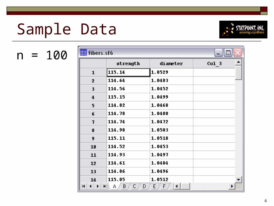
6

Sample Data

n = 100

7

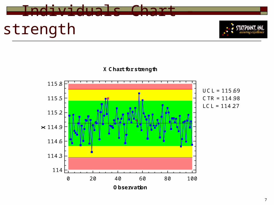
Individuals Chart - strength

X Chart for strength

0 20 40 60 80 100

Observation

114

114.3

114.6

114.9

115.2

115.5

115.8

X

CTR = 114.98UCL = 115.69

LCL = 114.27

8

Individuals Chart - diameter

X Chart for diameter

0 20 40 60 80 100

Observation

1.04

1.043

1.046

1.049

1.052

1.055

1.058

X

CTR = 1.05UCL = 1.06

LCL = 1.04

9

Capability Analysis - strength

NormalMean=114.978Std. Dev.=0.238937

Cp = 1.41Pp = 1.40Cpk = 1.38Ppk = 1.36K = -0.02

Process Capability for strength

LSL = 114.0, Nominal = 115.0, USL = 116.0

114 114.4 114.8 115.2 115.6 116

strength

0

4

8

12

16

20

24

freq

uenc

y

DPM = 30.76

10

Capability Analysis - diameter

DPM = 44.59

NormalMean=1.04991Std. Dev.=0.00244799

Cp = 1.41Pp = 1.36Cpk = 1.39Ppk = 1.35K = -0.01

Process Capability for diameter

LSL = 1.04, Nominal = 1.05, USL = 1.06

1.04 1.044 1.048 1.052 1.056 1.06diameter

0

4

8

12

16

20

freq

uenc

y

11

Scatterplot

Plot of strength vs diameter

1.04 1.045 1.05 1.055 1.06diameter

114

114.5

115

115.5

116

str

en

gth

correlation = 0.89

12

Multivariate Normal Distribution

Multivariate Normal Distribution

114 114.5 115 115.5 116

strength

1.041.045

1.051.055

1.06

diameter

13

Control Ellipse

Control Ellipse

1.04 1.043 1.046 1.049 1.052 1.055 1.058diameter

114

114.3

114.6

114.9

115.2

115.5

115.8

stre

ng

th

14

Multivariate Capability

Determines joint probability of being within the specification limits on all characteristics

Observed Estimated Estimated Variable Beyond Spec. Beyond Spec. DPM strength 0.0% 0.00307572% 30.7572 diameter 0.0% 0.00445939% 44.5939 Joint 0.0% 0.00703461% 70.3461

15

Multivariate Capability

Multivariate Normal DistributionDPM = 70.3461

113.5 114 114.5 115 115.5 116 116.5

strength

1.0351.041.0451.051.0551.061.065

diameter

16

Capability Ellipse

99.73% Capability Ellipse

MCP =1.27

113.5 114 114.5 115 115.5 116 116.5strength

1.035

1.04

1.045

1.05

1.055

1.06

1.065

diam

eter

17

Mult. Capability Indices

Defined to give the

same DPM as in the

univariate case.

Capability Indices Index Estimate MCP 1.27 MCR 78.80 DPM 70.3461 Z 3.80696 SQL 5.30696

18

Test for Normality

Probability Plot

-2.6 -1.6 -0.6 0.4 1.4 2.4 3.4normal distribution

-2.6

-1.6

-0.6

0.4

1.4

2.4

3.4

empi

rical

dat

a

strengthdiameter

P-Values Shapiro-Wilk strength 0.408004 diameter 0.615164

19

More than 2 Characteristics

Calculate T-squared:

where

S = sample covariance matrix

= vector of sample means

)()( 12 xxSxxT iii

x

20

T-Squared Chart

Multivariate Control Chart

UCL = 11.25

0 20 40 60 80 100 120Observation

0

5

10

15

20

25

30

T-S

quar

ed

21

T-Squared Decomposition

Subtracts the value of T-squared if each variable is removed.

Large values indicate that a variable has an important contribution.

T-Squared Decomposition Relative Contribution to T-Squared Signal Observation T-Squared diameter strength 17 26.3659 22.9655 25.951

22

Control Ellipsoid

Control Ellipsoid

1.04 1.044 1.048 1.052 1.056 1.06

diameter

114114.4114.8

115.2115.6

116

strength

6.8

7.8

8.8

9.8

10.8

11.8

12.8

rnor

mal

(100

,10,

1)

23

Multivariate EWMA Chart

Multivariate EWMA Control Chart

UCL = 11.25, lambda = 0.2

0 20 40 60 80 100 120

Observation

0

3

6

9

12

15

T-S

quar

ed

Largeststrengthdiameter

24

Generalized Variance Chart

Plots the determinant of the variance-covariance matrix for data that is sampled in subgroups.

Generalized Variance Chart

0 4 8 12 16 20 24

Subgroup

0

1

2

3

4

5

6(X 1.E-7)

Gen

. Var

ianc

e

UCL = 3.281E-7CL = 7.01937E-8LCL = 0.0

25

Data Exploration and Modeling

When the number of variables is large, the dimensionality of the problem often makes it difficult to determine the underlying relationships.

Reduction of dimensionality can be very helpful.

26

Example #2

27

Matrix PlotMPG City

MPG Highway

Engine Size

Horsepower

Fueltank

Passengers

Length

Wheelbase

Width

U Turn Space

Weight

28

Analysis Methods

Predicting certain characteristics based on others (regression and ANOVA)

Separating items into groups (classification)

Detecting unusual items

29

Multiple RegressionMPG City = 29.6315 + 0.28816*Engine Size - 0.00688362*Horsepower - 0.297446*Passengers - 0.0365723*Length + 0.280224*Wheelbase + 0.111526*Width - 0.139763*U Turn Space - 0.00984486*Weight Standard T Parameter Estimate Error Statistic P-Value CONSTANT 29.6315 12.9763 2.28351 0.0249 Engine Size 0.28816 0.722918 0.398607 0.6912 Horsepower -0.00688362 0.0134153 -0.513119 0.6092 Passengers -0.297446 0.54754 -0.543241 0.5884 Length -0.0365723 0.0447211 -0.817786 0.4158 Wheelbase 0.280224 0.124837 2.24472 0.0274 Width 0.111526 0.218893 0.5095 0.6117 U Turn Space -0.139763 0.17926 -0.779668 0.4378 Weight -0.00984486 0.00192619 -5.11104 0.0000 R-squared = 73.544 percent R-squared (adjusted for d.f.) = 71.0244 percent Standard Error of Est. = 3.02509 Mean absolute error = 1.99256

30

Principal Components

The goal of a principal components analysis (PCA) is to construct k linear combinations of the p variables X that contain the greatest variance.

pp XaXaXaC 12121111 ...

pp XaXaXaC 22221212 ...

…

pkpkkk XaXaXaC ...2211

31

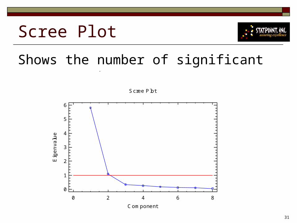
Scree Plot

Shows the number of significant components.

Scree Plot

Component

Eig

en

valu

e

0 2 4 6 80

1

2

3

4

5

6

32

Percentage Explained

Principal Components Analysis Component Percent of Cumulative Number Eigenvalue Variance Percentage 1 5.8263 72.829 72.829 2 1.09626 13.703 86.532 3 0.339796 4.247 90.779 4 0.270321 3.379 94.158 5 0.179286 2.241 96.400 6 0.12342 1.543 97.942 7 0.109412 1.368 99.310 8 0.0552072 0.690 100.000

33

ComponentsTable of Component Weights Component Component 1 2 Engine Size 0.376856 -0.205144 Horsepower 0.292144 -0.592729 Passengers 0.239193 0.730749 Length 0.369908 0.0429221 Wheelbase 0.374826 0.259648 Width 0.38949 -0.0422083 U Turn Space 0.359702 -0.0256716 Weight 0.396236 -0.0298902

First component 0.376856*Engine Size + 0.292144*Horsepower + 0.239193*Passengers + 0.369908*Length + 0.374826*Wheelbase + 0.38949*Width + 0.359702*U Turn Space + 0.396236*Weight Second component -0.205144*Engine Size – 0.592729*Horsepower + 0.730749*Passengers + 0.0429221*Length + 0.259648*Wheelbase - 0.0422083*Width - 0.0256716*U Turn Space – 0.0298902*Weight

34

Interpretation

Plot of C_2 vs C_1

C_1

C_2

TypeCompactLarge MidsizeSmall Sporty Van

-6 -4 -2 0 2 4 6-5

-3

-1

1

3

35

Principal Component RegressionMPG City = 22.3656 - 1.84685*size + 0.567176*unsportiness Standard T Parameter Estimate Error Statistic P-Value CONSTANT 22.3656 0.353316 63.302 0.0000 size -1.84685 0.147168 -12.5492 0.0000 unsportiness 0.567176 0.339277 1.67172 0.0981 R-squared = 64.0399 percent R-squared (adjusted for d.f.) = 63.2408 percent Standard Error of Est. = 3.40726 Mean absolute error = 2.26553

36

Partial Least Squares (PLS)

Similar to PCA, except that it finds components that minimize the variance in both the X’s and the Y’s.

May be used with many X variables, even exceeding n.

37

Component Extraction

Starts with number of components equal to the minimum of p and (n-1).

Model Comparison Plot

Number of components

Pe

rce

nt

vari

ati

on

XY

1 2 3 4 5 6 7 80

20

40

60

80

100

38

Coefficient Plot

PLS Coefficient Plot

Stn

d.

coe

ffic

ien

t

MPG CityMPG HighwayFueltank

-0.7

-0.5

-0.3

-0.1

0.1

0.3

0.5E

ng

ine

Siz

e

Ho

rse

po

we

r

Pa

sse

ng

ers

Le

ng

th

Wh

ee

lba

se

Wid

th

U T

urn

Sp

ace

We

igh

t

39

Model in Original Units

MPG City = 50.0593 – 0.214083*Engine Size - 0.0347708*Horsepower

- 0.884181*Passengers + 0.0294622*Length - 0.0362471*Wheelbase

- 0.0882233*Width - 0.0282326*U Turn Space - 0.00391616*Weight

40

Classification

Principal components can also be used to classify new observations.

A useful method for classification is a Bayesian classifier, which can be expressed as a neural network.

41

6 Types of Automobiles

Plot of unsportiness vs size

size

un

spo

rtin

ess

TypeCompactLarge MidsizeSmall Sporty Van

-6 -4 -2 0 2 4 6-5

-3

-1

1

3

42

Neural Networks

Input layer

(2 variables)

Pattern layer

(93 cases)

Summation layer

(6 neurons)

Output layer

(6 groups)

43

Bayesian Classifier Begins with prior probabilities for membership in

each group

Uses a Parzen-like density estimator of the density function for each group

jn

i

i

jj

XX

nXg

12

2

exp1

)(

44

Options

The prior probabilities may be determined in several ways.

A training set is usually used to find a good value for .

45

OutputNumber of cases in training set: 93 Number of cases in validation set: 0 Spacing parameter used: 0.0109375 (optimized by jackknifing during training) Training Set Percent Correctly Type Members Classified Compact 16 75.0 Large 11 100.0 Midsize 22 77.2727 Small 21 76.1905 Sporty 14 85.7143 Van 9 100.0 Total 93 82.7957

46

Classification Regions

Classification Plot

size

unsp

ortin

ess

TypeCompact Large Midsize Small Sporty Van

sigma = 0.0109375

-6 -4 -2 0 2 4 6-5

-3

-1

1

3

47

Changing Sigma

Classification Plot

size

unsp

ortin

ess

TypeCompact Large Midsize Small Sporty Van

-6 -4 -2 0 2 4 6-5

-3

-1

1

3

sigma = 0.3

48

Overlay Plot

Classification Plot

size

un

spo

rtin

ess

TypeCompact Large Midsize Small Sporty Van

sigma = 0.3

-6 -4 -2 0 2 4 6-5

-3

-1

1

3

49

Outlier Detection

Control Ellipse

size

unsp

ortin

ess

-8 -4 0 4 8-5

-3

-1

1

3

5

50

Cluster Analysis

Cluster Scatterplot

Method of k-Means,Squared Euclidean

-6 -4 -2 0 2 4 6

size

-5

-3

-1

1

3

unsp

ortin

ess

Cluster 1234Centroids

51

Design of Experiments

When more than one characteristic is important, finding the optimal operating conditions usually requires a tradeoff of one characteristic for another.

One approach to finding a single solution is to use desirability functions.

52

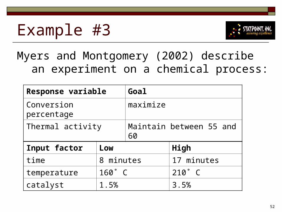
Example #3

Myers and Montgomery (2002) describe an experiment on a chemical process:

Response variable Goal

Conversion percentage maximize

Thermal activity Maintain between 55 and 60

Input factor Low High

time 8 minutes 17 minutes

temperature 160˚ C 210˚ C

catalyst 1.5% 3.5%

53

Experimentrun time temperature catalyst conversion activity (minutes ) (degrees C ) (percent ) 1 10.0 170.0 2.0 74.0 53.2 2 15.0 170.0 2.0 51.0 62.9 3 10.0 200.0 2.0 88.0 53.4 4 15.0 200.0 2.0 70.0 62.6 5 10.0 170.0 3.0 71.0 57.3 6 15.0 170.0 3.0 90.0 67.9 7 10.0 200.0 3.0 66.0 59.8 8 15.0 200.0 3.0 97.0 67.8 9 8.3 185.0 2.5 76.0 59.1 10 16.7 185.0 2.5 79.0 65.9 11 12.5 160.0 2.5 85.0 60.0 12 12.5 210.0 2.5 97.0 60.7 13 12.5 185.0 1.66 55.0 57.4 14 12.5 185.0 3.35 81.0 63.2 15 12.5 185.0 2.5 81.0 59.2 16 12.5 185.0 2.5 75.0 60.4 17 12.5 185.0 2.5 76.0 59.1 18 12.5 185.0 2.5 83.0 60.6 19 12.5 185.0 2.5 80.0 60.8 20 12.5 185.0 2.5 91.0 58.9

54

Step #1: Model Conversion

Standardized Pareto Chart for conversion

0 2 4 6 8

Standardized effect

A:timeABAABCBB

B:temperatureCC

C:catalystAC +

-

55

Step #2: Optimize ConversionGoal: maximize conversion Optimum value = 118.174 Factor Low High Optimum time 8.0 17.0 17.0 temperature 160.0 210.0 210.0 catalyst 1.5 3.5 3.48086

Contours of Estimated Response Surfacetemperature=210.0

8 9 10 11 12 13 14 15 16 17

time

1.5

2

2.5

3

3.5

cata

lyst

conversion70.072.575.077.580.082.585.087.590.092.595.097.5100.0

56

Step #3: Model Activity

Standardized Pareto Chart for activity

0 2 4 6 8

Standardized effect

ACCCBBBC

B:temperatureABAA

C:catalystA:time +

-

57

Step #4: Optimize ActivityGoal: maintain activity at 57.5 Optimum value = 57.5 Factor Low High Optimum time 8.3 16.7 10.297 temperature 209.99 210.01 210.004 catalyst 1.66 3.35 2.31021

Contours of Estimated Response Surface

temperature=210.0

8 9 10 11 12 13 14 15 16 17

time

1.5

2

2.5

3

3.5

cata

lyst

activity55.056.057.058.059.060.0

58

Step #5: Select Desirability Fcns.

Maximize

Desirability Function for Maximization

Predicted response

Desir

abili

ty, d

s = 1s = 2

s = 8

s = 0.4

s = 0.2

Low

0 20 40 60 80 100

0

0.2

0.4

0.6

0.8

1

High

59

Desirability Function

Hit Target

Desirability Function for Hitting Target

Predicted response

Desir

abilit

y, d

Low HighTarget

s = 1 t = 1

s = 0.1 t = 0.1

s = 5

0 20 40 60 80 1000

0.2

0.4

0.6

0.8

1

t = 5

60

Combined Desirability

where m = # of factors and 0 ≤ Ij ≤ 5. D ranges from 0 to 1.

m

jjm

IIm

II dddD 121

/1

21 ...

61

ExampleOptimum value = 0.949092 Factor Low High Optimum time 8.0 17.0 11.1394 temperature 160.0 210.0 210.0 catalyst 1.5 3.5 2.20119

Weights Weights Response Low High Goal First Second Impact conversion 50.0 100.0 Maximize 1.0 3.0 activity 55.0 60.0 57.5 1.0 1.0 3.0

Response Optimum conversion 95.0388 activity 57.5

62

Desirability Contours

Contours of Estimated Response Surfacetemperature=210.0

8 9 10 11 12 13 14 15 16 17

time

1.5

2

2.5

3

3.5

cata

lyst

Desirability0.00.10.20.30.40.50.60.70.80.91.0

63

Desirability Surface

Estimated Response Surfacetemperature=210.0

8 9 10 11 12 13 14 15 16 17time

1.52

2.53

3.5

catalyst

0

0.2

0.4

0.6

0.8

1

Des

irab

ility

64

Overlaid Contours

Overlay Plottemperature=210.0

conversionactivity

10 11 12 13 14 15

time

2

2.2

2.4

2.6

2.8

3

cata

lyst

65

References Johnson, R.A. and Wichern, D.W. (2002). Applied Multivariate

Statistical Analysis. Upper Saddle River: Prentice Hall.Mason, R.L. and Young, J.C. (2002).

Mason and Young (2002). Multivariate Statistical Process Control with Industrial Applications. Philadelphia: SIAM.

Montgomery, D. C. (2005). Introduction to Statistical Quality Control, 5th edition. New York: John Wiley and Sons.

Myers, R. H. and Montgomery, D. C. (2002). Response Surface Methodology: Process and Product optimization Using Designed Experiments, 2nd edition. New York: John Wiley and Sons.

66

PowerPoint Slides

Available at:

www.statgraphics.com/documents.htm