Multivariate Data Analysis Using

Statgraphics Centurion: Part 3

Dr. Neil W. Polhemus

Statpoint Technologies, Inc.

1

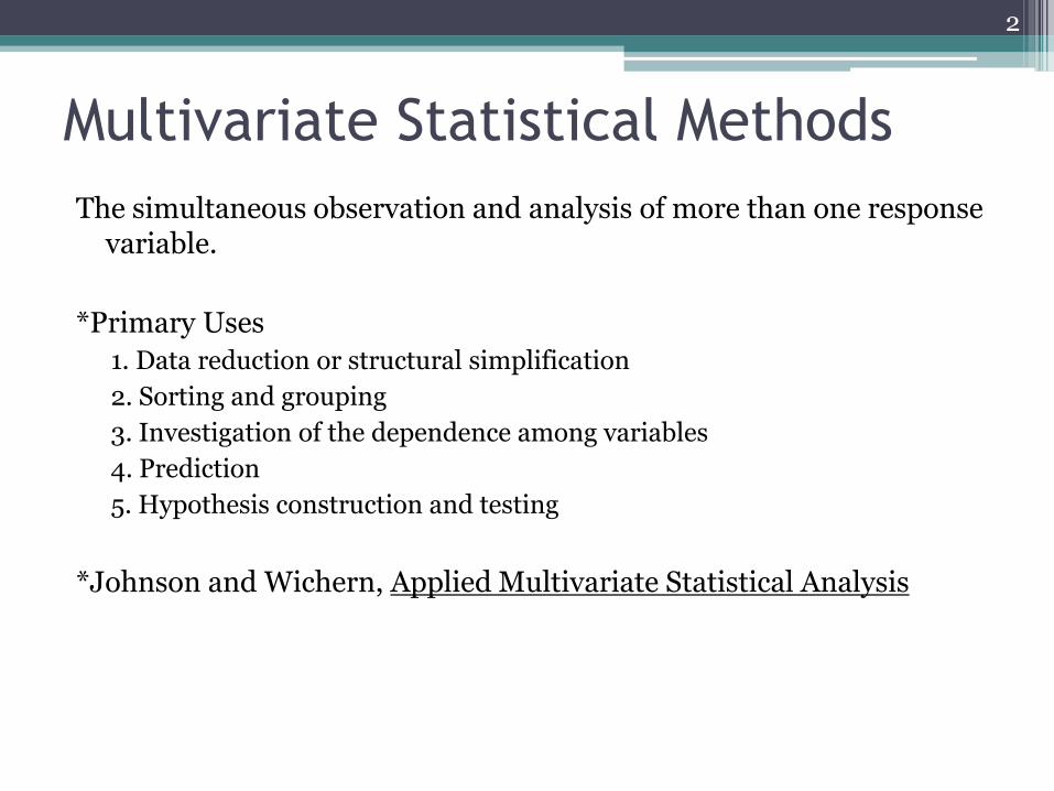
Multivariate Statistical Methods

The simultaneous observation and analysis of more than one response variable.

*Primary Uses

1. Data reduction or structural simplification

2. Sorting and grouping

3. Investigation of the dependence among variables

4. Prediction

5. Hypothesis construction and testing

*Johnson and Wichern, Applied Multivariate Statistical Analysis

2

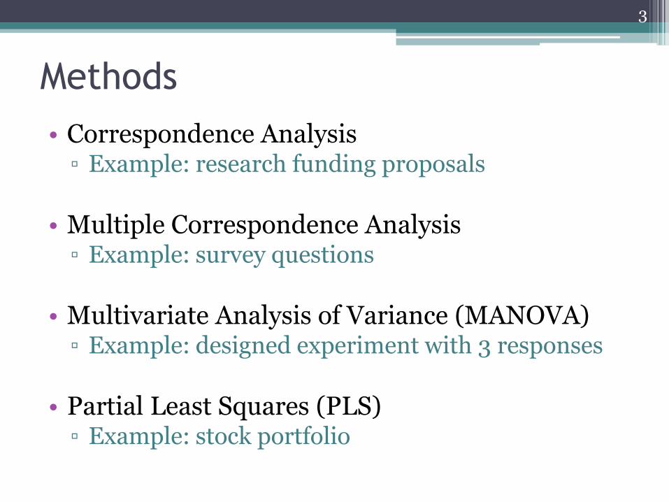
Methods

• Correspondence Analysis ▫ Example: research funding proposals

• Multiple Correspondence Analysis

▫ Example: survey questions

• Multivariate Analysis of Variance (MANOVA)

▫ Example: designed experiment with 3 responses

• Partial Least Squares (PLS)

▫ Example: stock portfolio

3

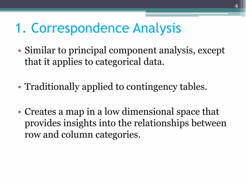
1. Correspondence Analysis

• Similar to principal component analysis, except that it applies to categorical data.

• Traditionally applied to contingency tables.

• Creates a map in a low dimensional space that provides insights into the relationships between row and column categories.

4

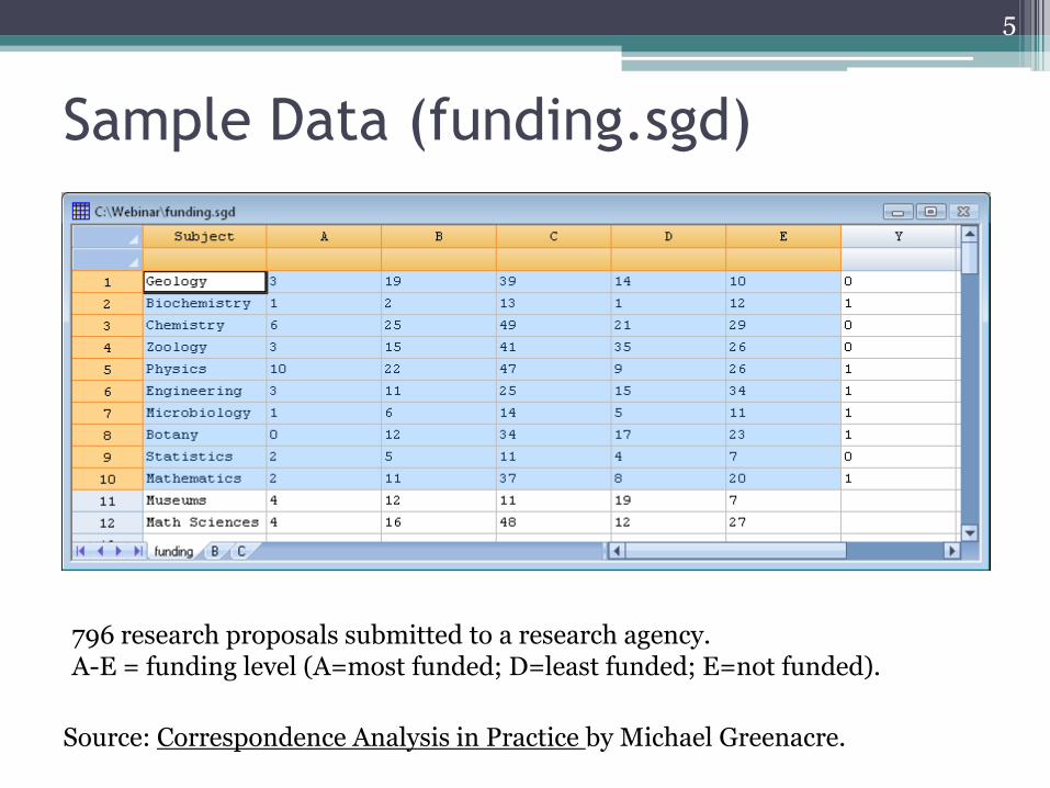
Sample Data (funding.sgd)

5

Source: Correspondence Analysis in Practice by Michael Greenacre.

796 research proposals submitted to a research agency. A-E = funding level (A=most funded; D=least funded; E=not funded).

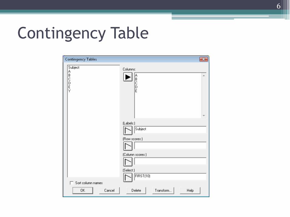
Contingency Table

6

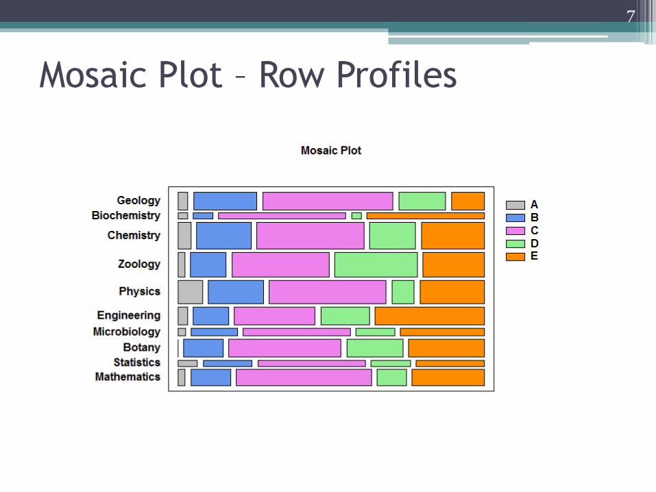
Mosaic Plot – Row Profiles

7

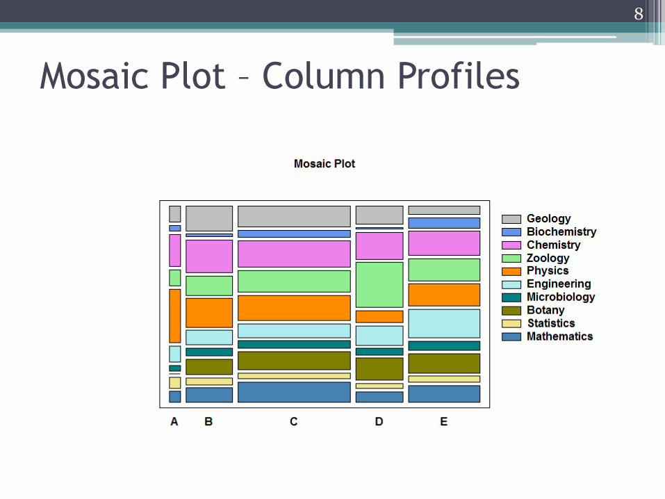
Mosaic Plot – Column Profiles

8

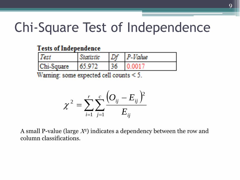
Chi-Square Test of Independence

9

A small P-value (large C2) indicates a dependency between the row and column classifications.

r

i

c

j ij

ijij

E

EO

1 1

2

2

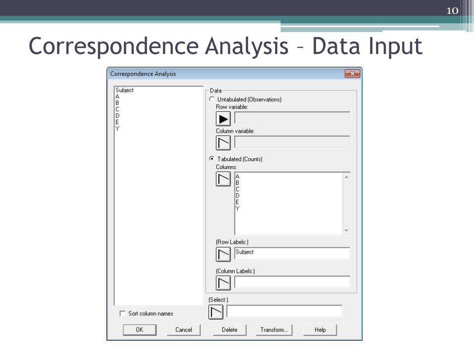
Correspondence Analysis – Data Input

10

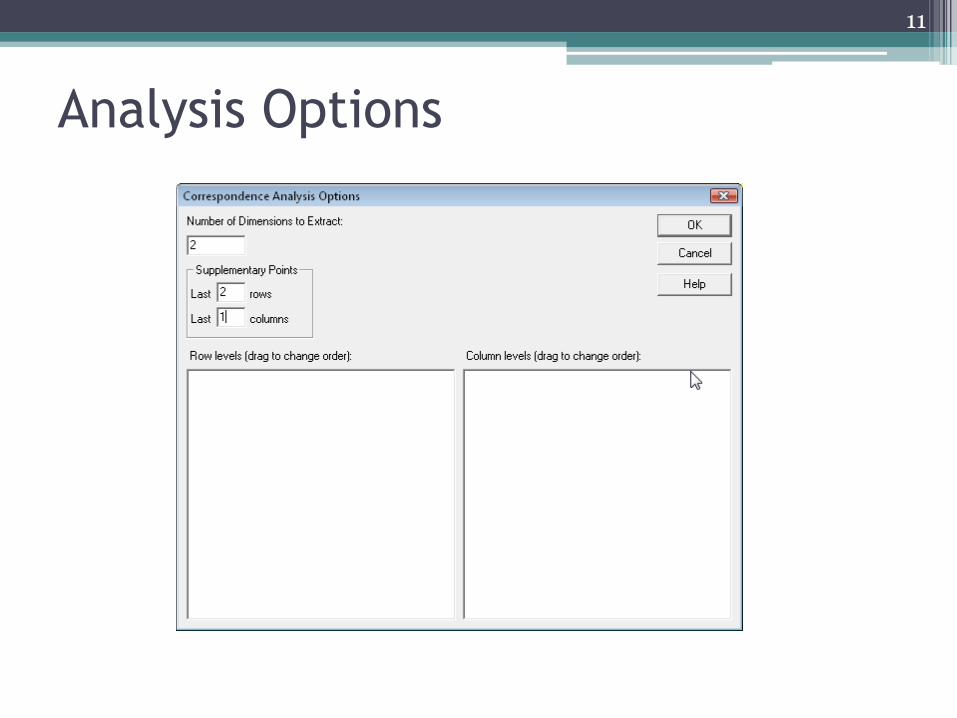
Analysis Options

11

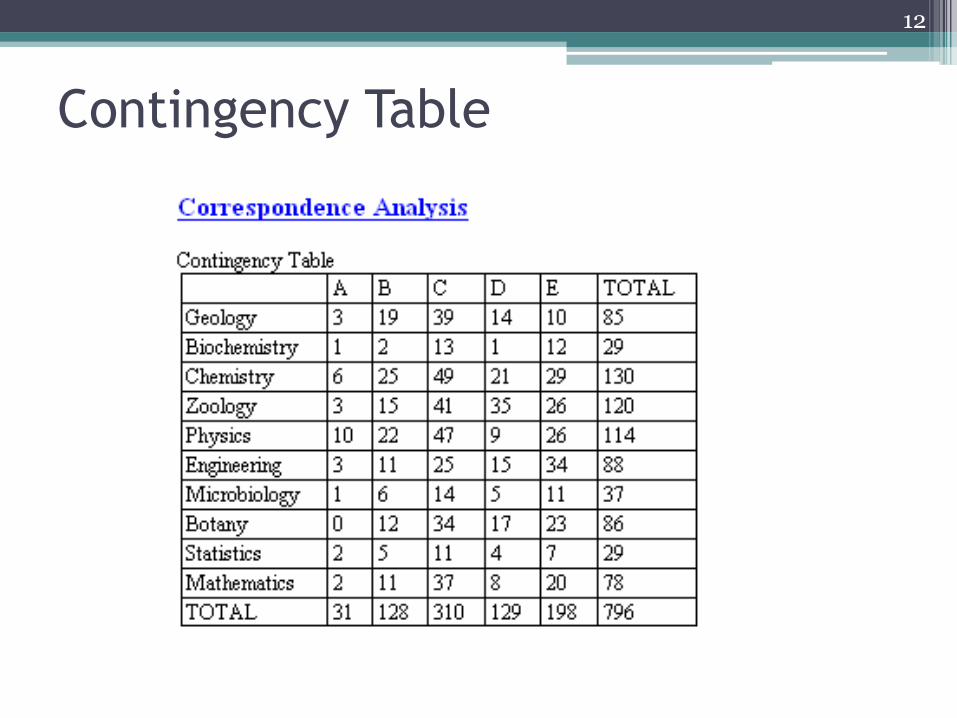
Contingency Table

12

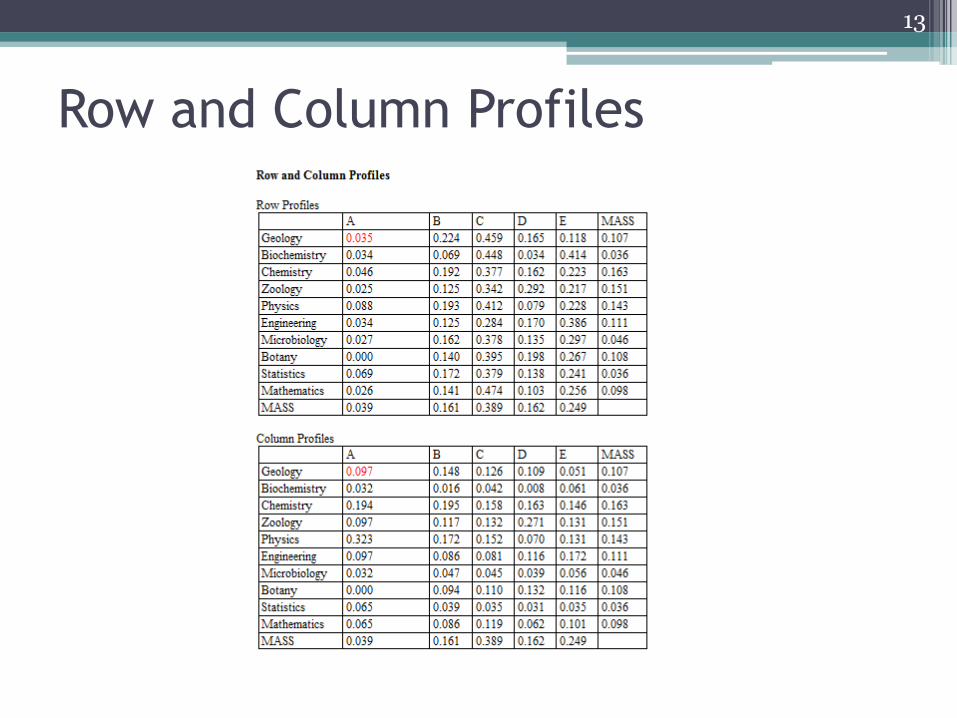
Row and Column Profiles

13

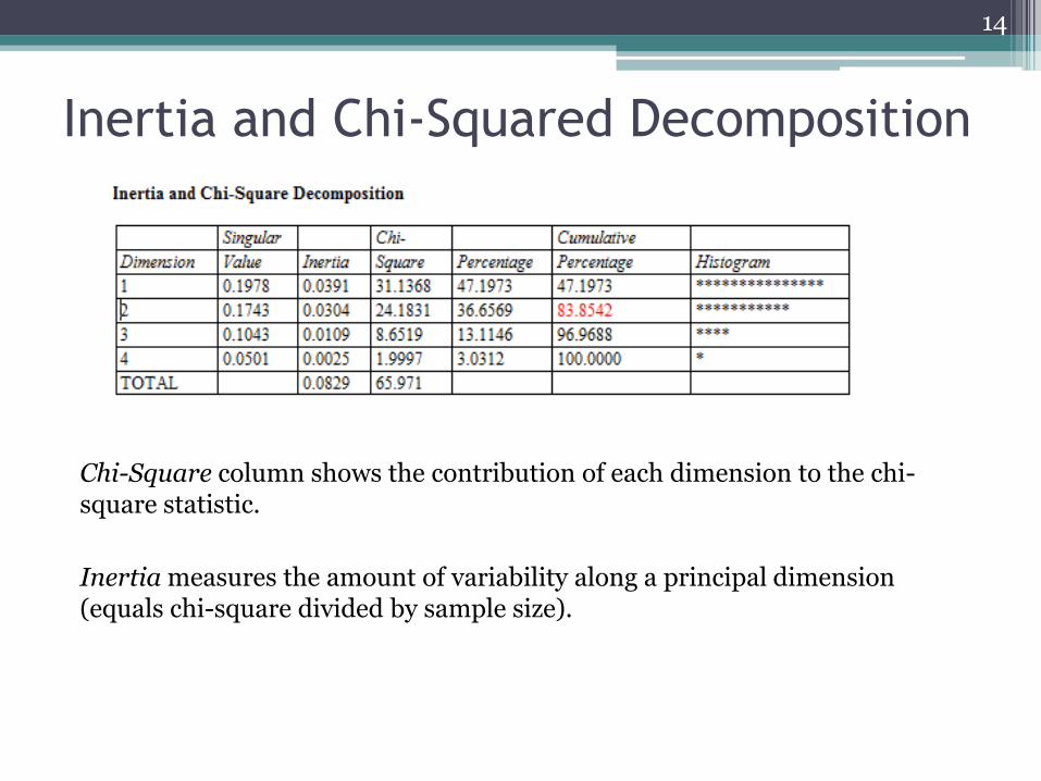
Inertia and Chi-Squared Decomposition

14

Inertia measures the amount of variability along a principal dimension (equals chi-square divided by sample size).

Chi-Square column shows the contribution of each dimension to the chi-square statistic.

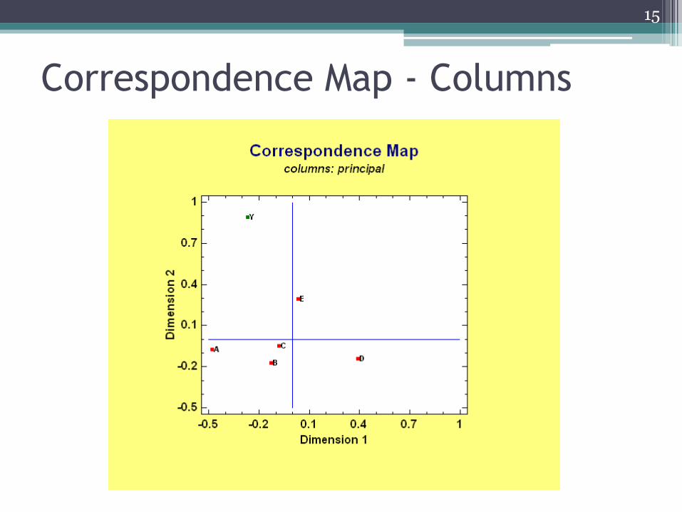
Correspondence Map - Columns

15

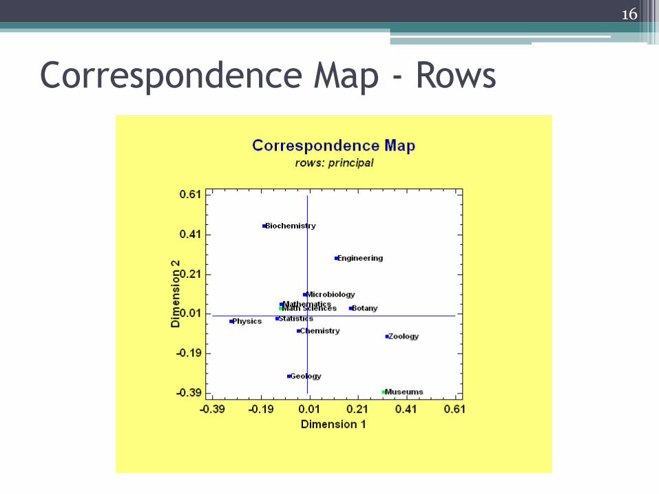
Correspondence Map - Rows

16

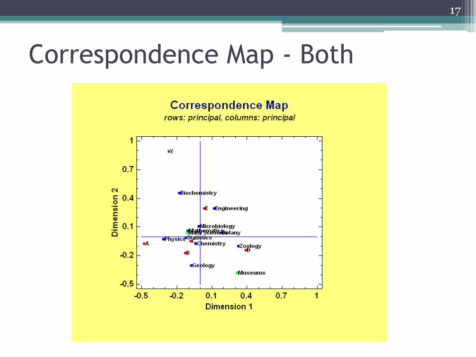
Correspondence Map - Both

17

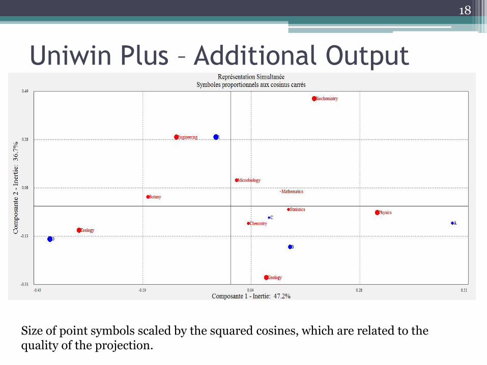
Uniwin Plus – Additional Output

18

Size of point symbols scaled by the squared cosines, which are related to the quality of the projection.

2. Multiple Correspondence Analysis

• Deals with the associations within one set of variables

• The goal is to understand how strongly and in what way the variables are related

19

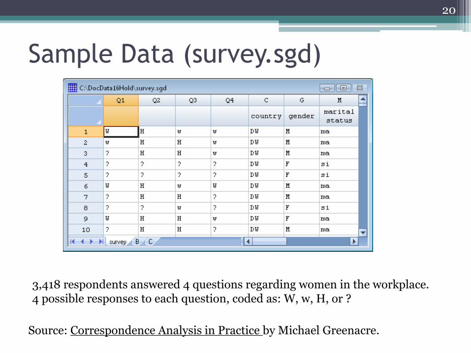
Sample Data (survey.sgd)

20

Source: Correspondence Analysis in Practice by Michael Greenacre.

3,418 respondents answered 4 questions regarding women in the workplace. 4 possible responses to each question, coded as: W, w, H, or ?

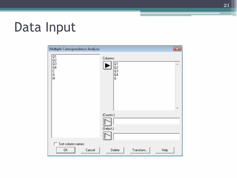
Data Input

21

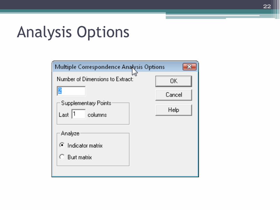
Analysis Options

22

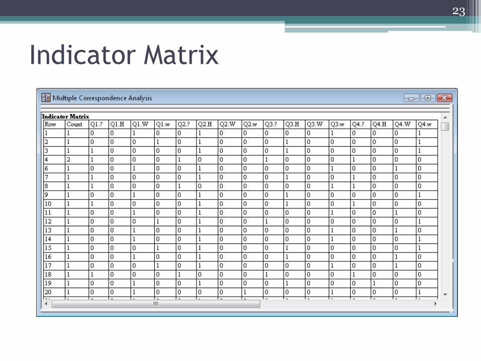
Indicator Matrix

23

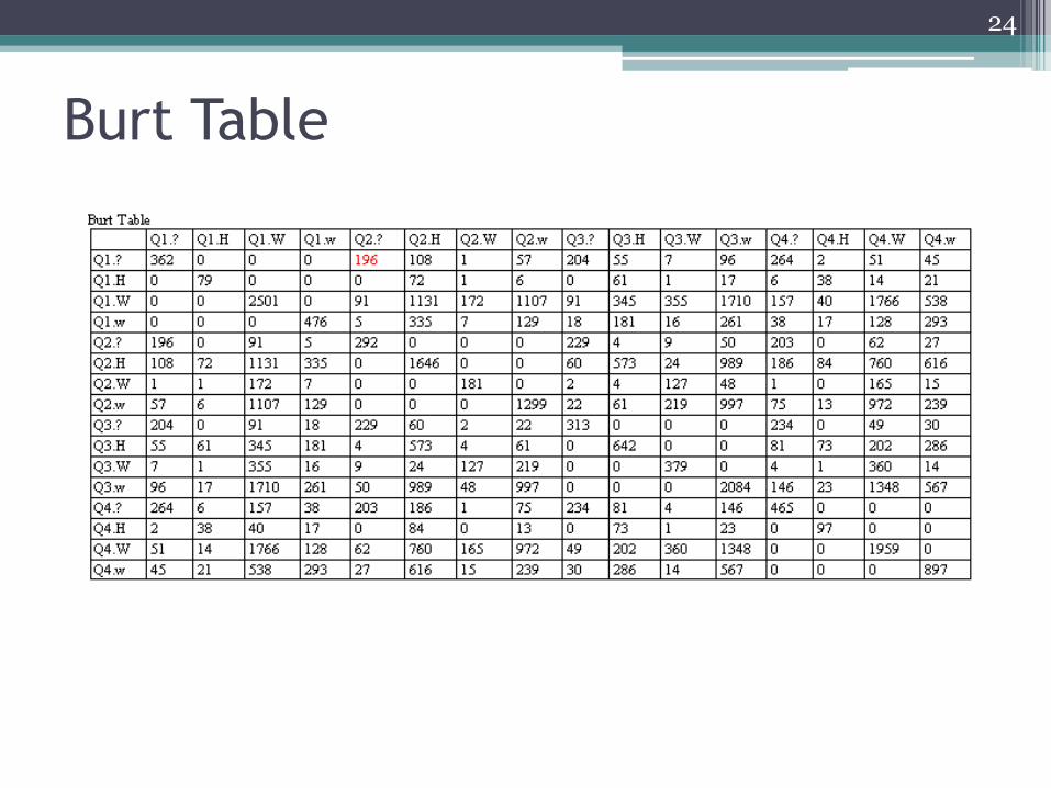
Burt Table

24

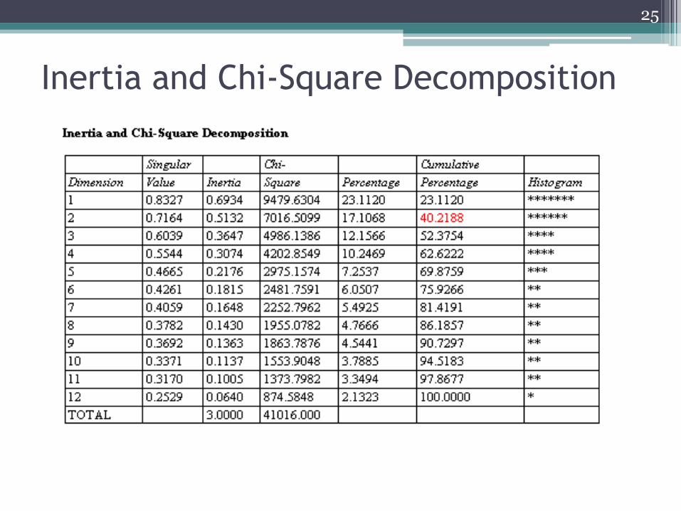
Inertia and Chi-Square Decomposition

25

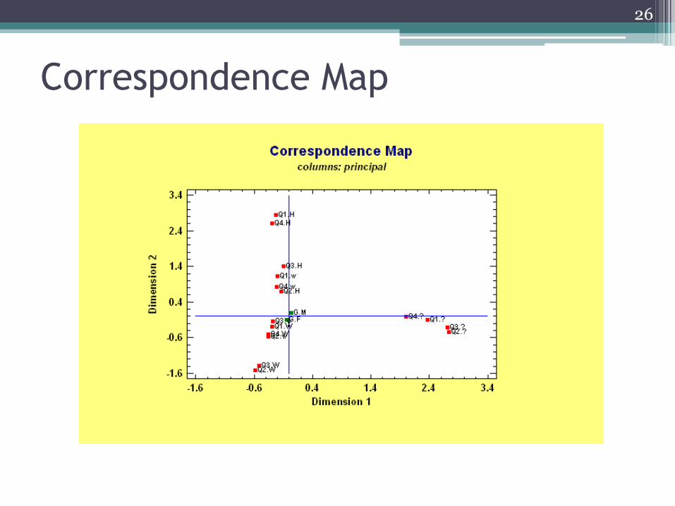
Correspondence Map

26

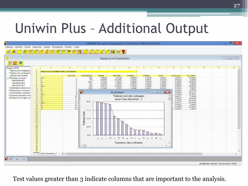
Uniwin Plus – Additional Output

27

Test values greater than 3 indicate columns that are important to the analysis.

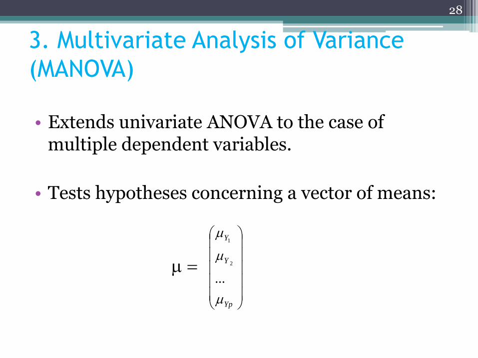
3. Multivariate Analysis of Variance

(MANOVA)

• Extends univariate ANOVA to the case of multiple dependent variables.

• Tests hypotheses concerning a vector of means:

m

28

Yp

Y

Y

m

m

m

...

2

1

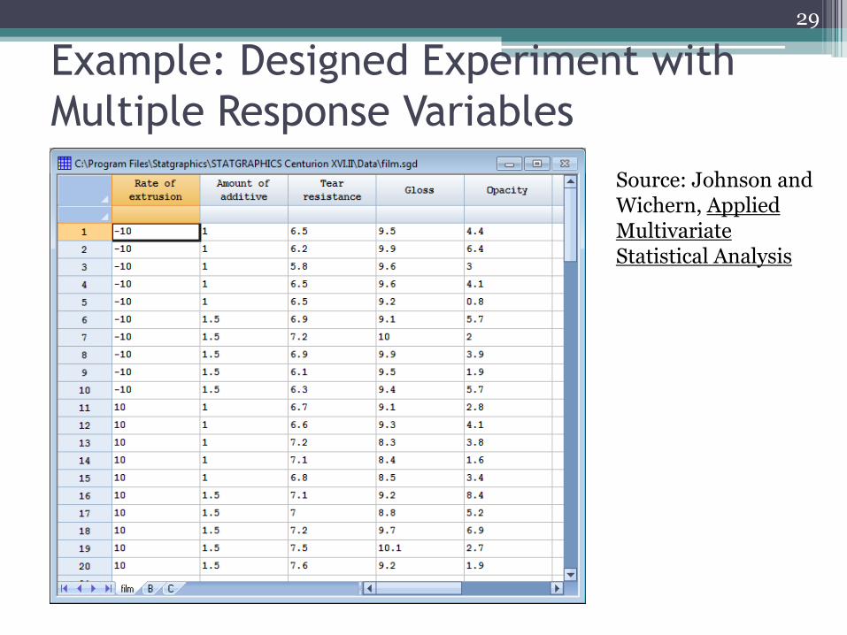
Example: Designed Experiment with

Multiple Response Variables

29

Source: Johnson and Wichern, Applied Multivariate Statistical Analysis

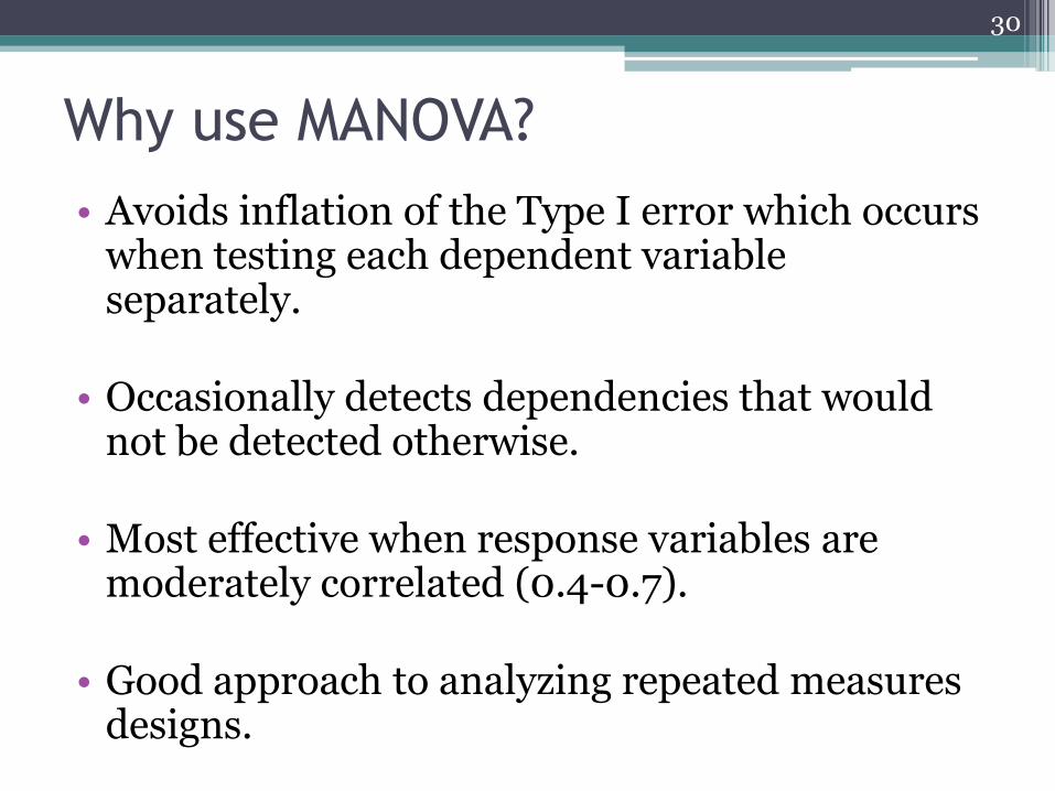
Why use MANOVA?

• Avoids inflation of the Type I error which occurs when testing each dependent variable separately.

• Occasionally detects dependencies that would not be detected otherwise.

• Most effective when response variables are moderately correlated (0.4-0.7).

• Good approach to analyzing repeated measures

designs.

30

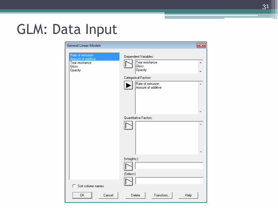
GLM: Data Input

31

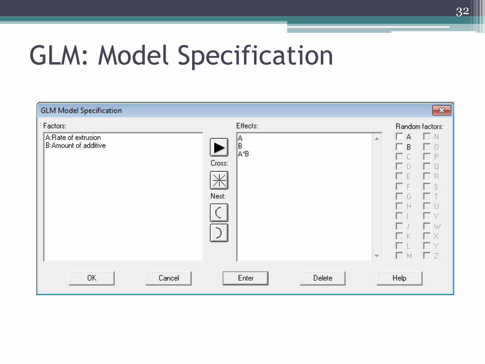
GLM: Model Specification

32

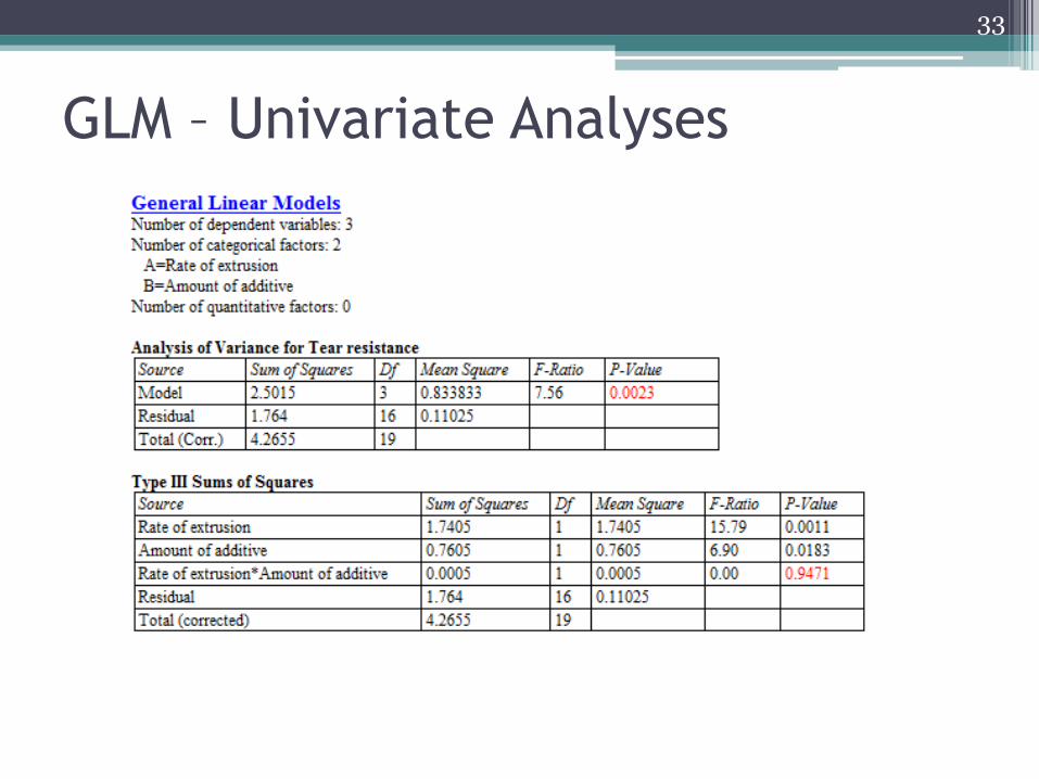
GLM – Univariate Analyses

33

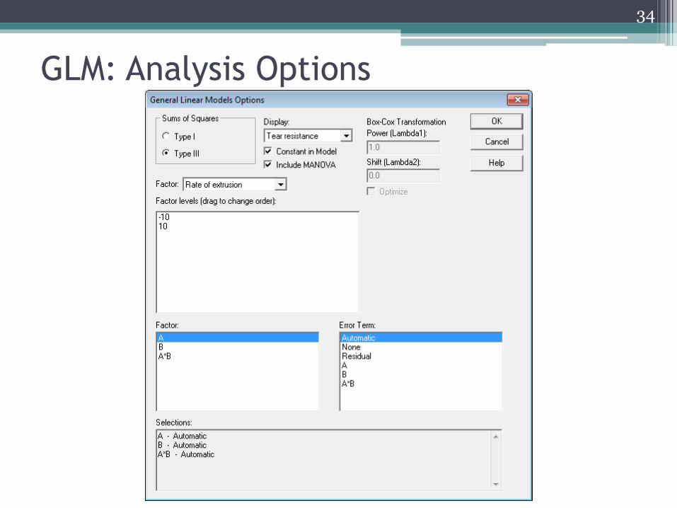
GLM: Analysis Options

34

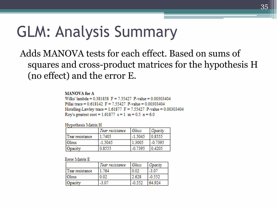
GLM: Analysis Summary

Adds MANOVA tests for each effect. Based on sums of squares and cross-product matrices for the hypothesis H (no effect) and the error E.

35

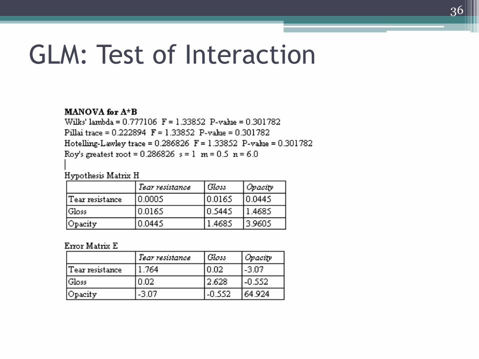
GLM: Test of Interaction

36

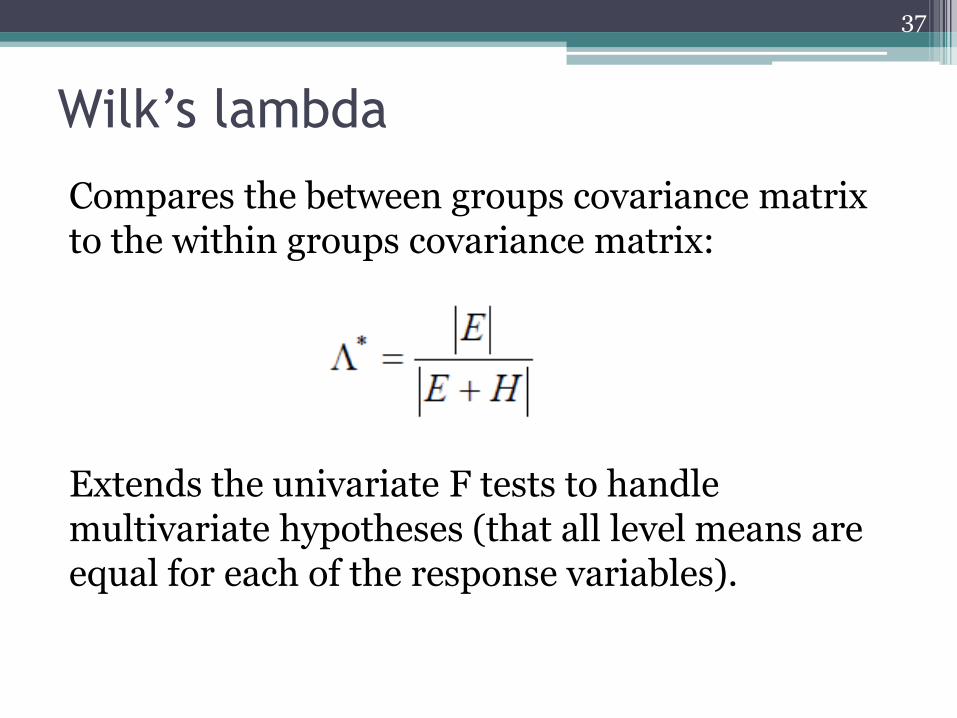
Wilk’s lambda

Compares the between groups covariance matrix to the within groups covariance matrix:

Extends the univariate F tests to handle multivariate hypotheses (that all level means are equal for each of the response variables).

37

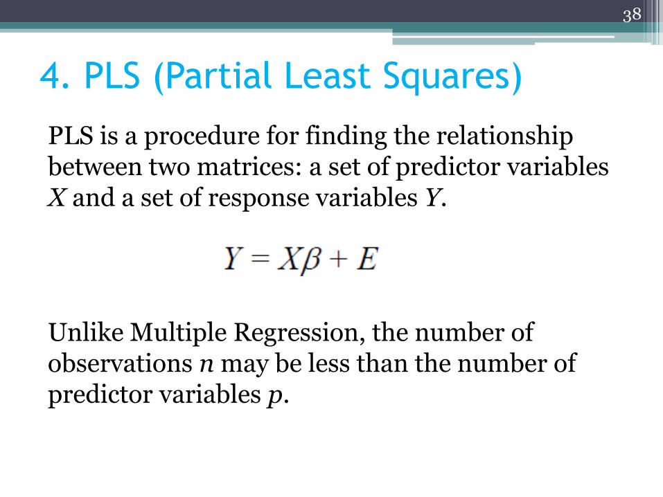
4. PLS (Partial Least Squares)

PLS is a procedure for finding the relationship between two matrices: a set of predictor variables X and a set of response variables Y.

Unlike Multiple Regression, the number of observations n may be less than the number of predictor variables p.

38

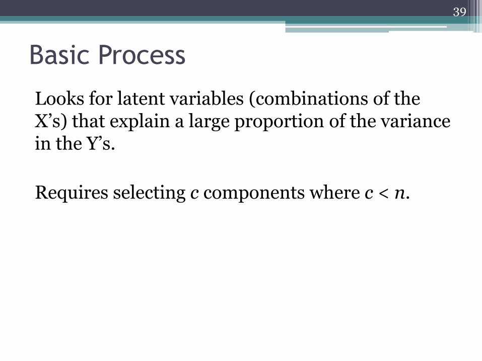
Basic Process

Looks for latent variables (combinations of the X’s) that explain a large proportion of the variance in the Y’s.

Requires selecting c components where c < n.

39

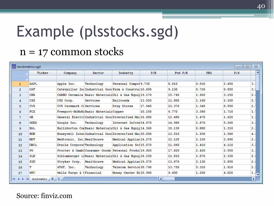
Example (plsstocks.sgd)

n = 17 common stocks

40

Source: finviz.com

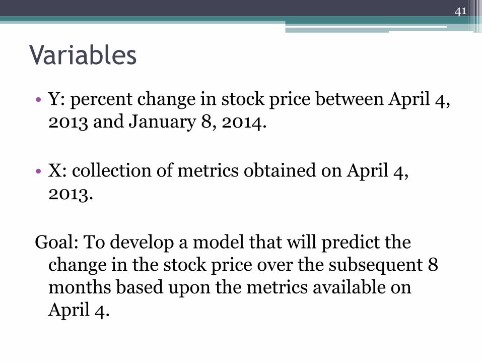
Variables

• Y: percent change in stock price between April 4, 2013 and January 8, 2014.

• X: collection of metrics obtained on April 4, 2013.

Goal: To develop a model that will predict the change in the stock price over the subsequent 8 months based upon the metrics available on April 4.

41

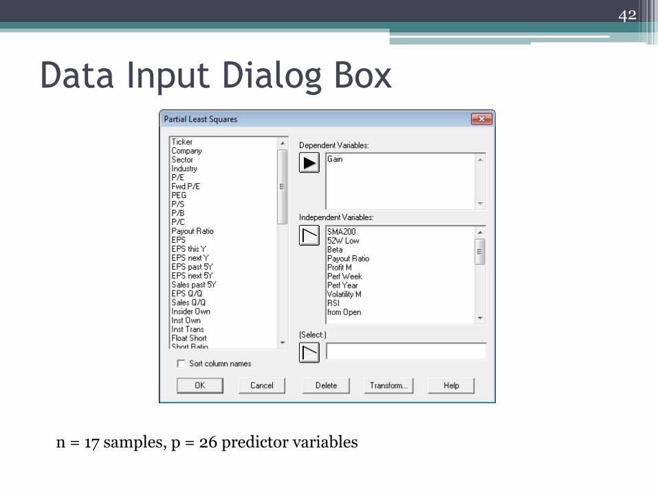
Data Input Dialog Box

42

n = 17 samples, p = 26 predictor variables

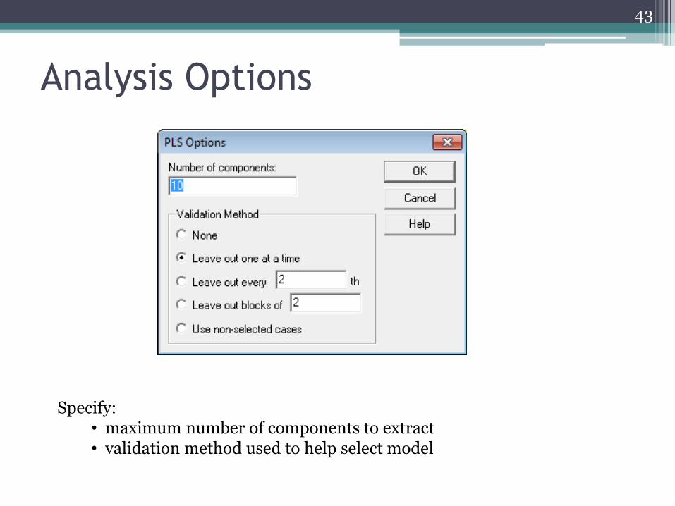
Analysis Options

43

Specify: • maximum number of components to extract • validation method used to help select model

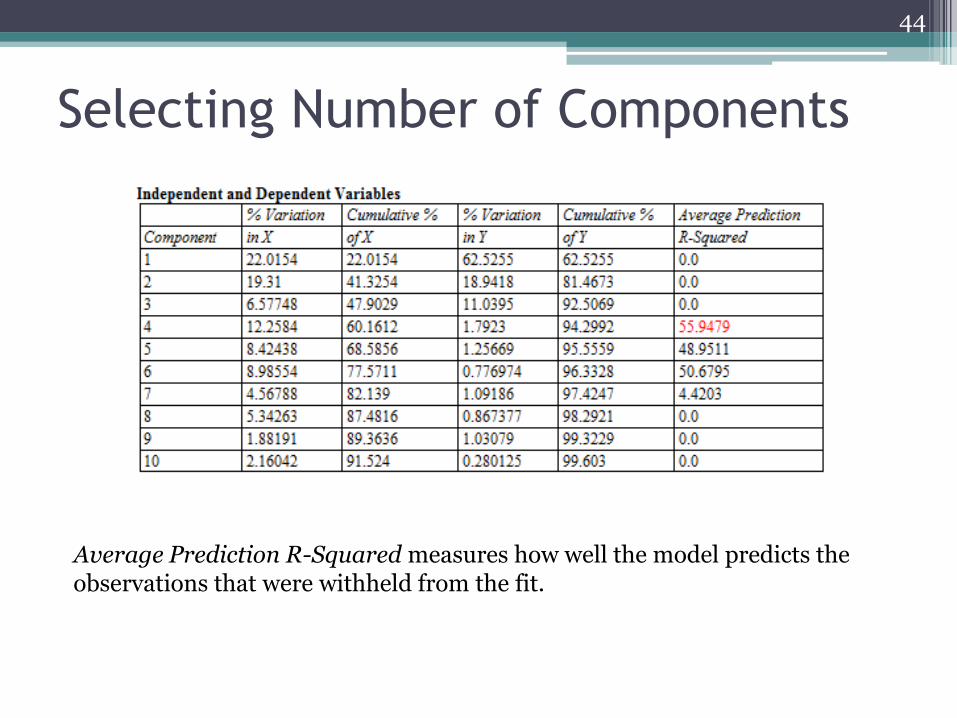
Selecting Number of Components

44

Average Prediction R-Squared measures how well the model predicts the observations that were withheld from the fit.

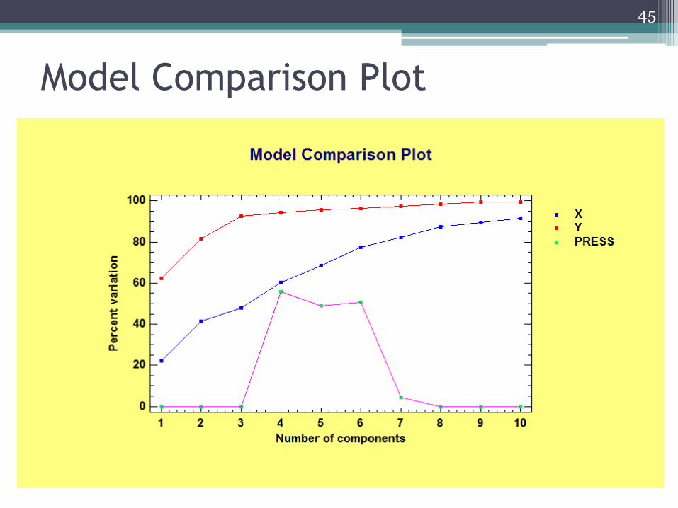
Model Comparison Plot

45

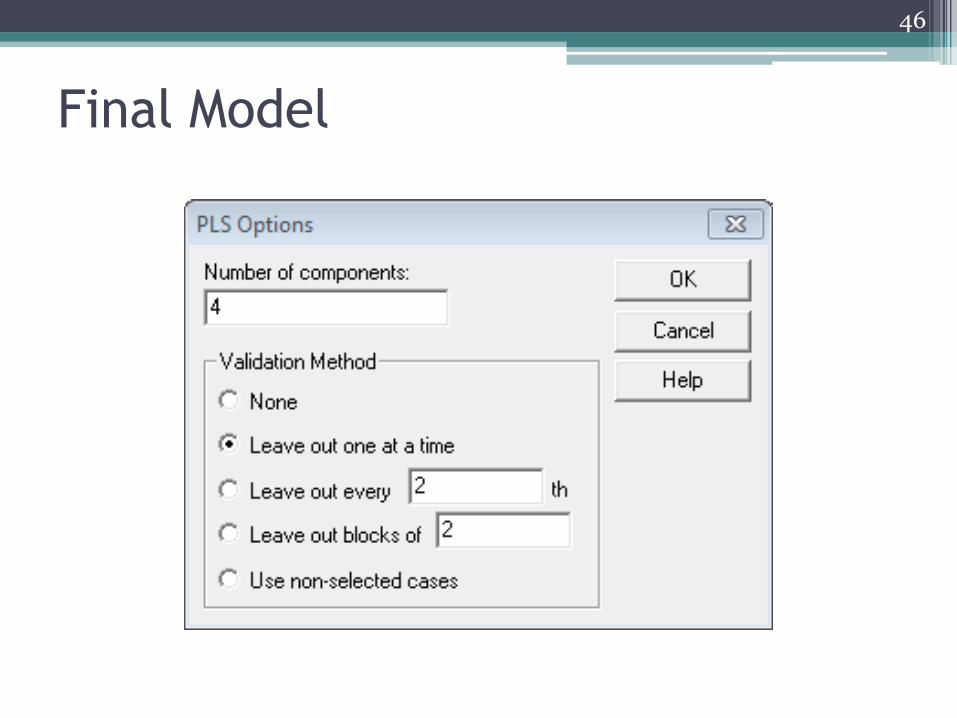
Final Model

46

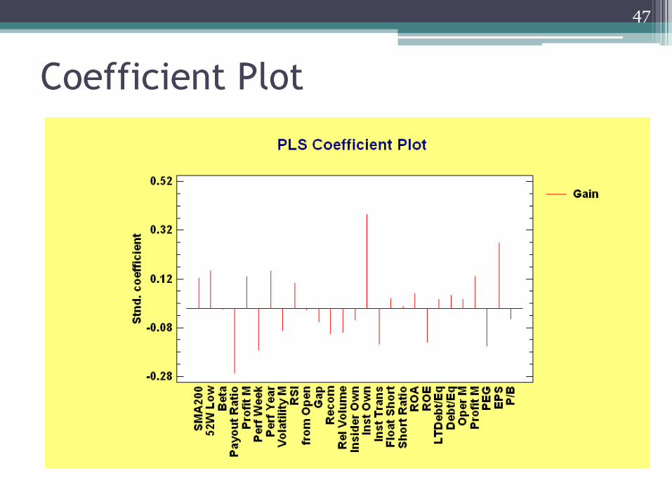
Coefficient Plot

47

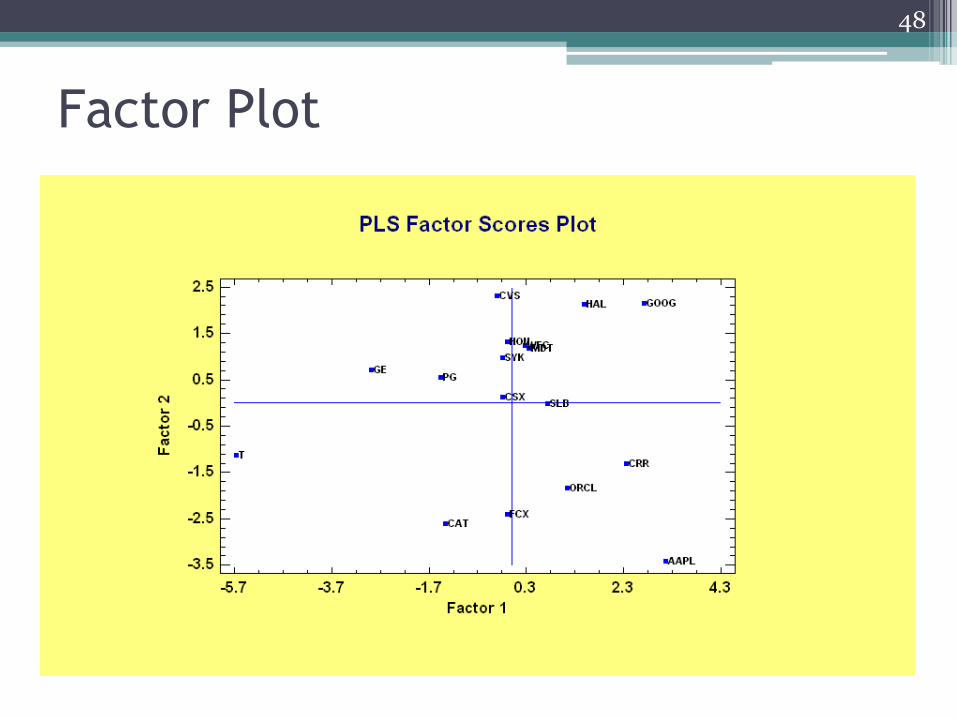
Factor Plot

48

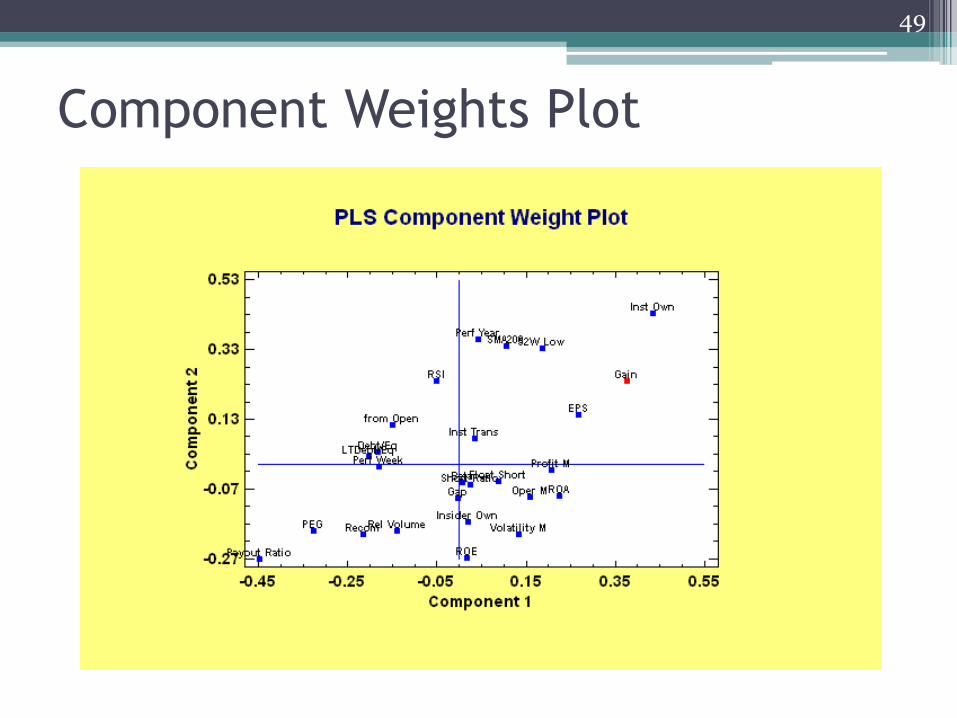
Component Weights Plot

49

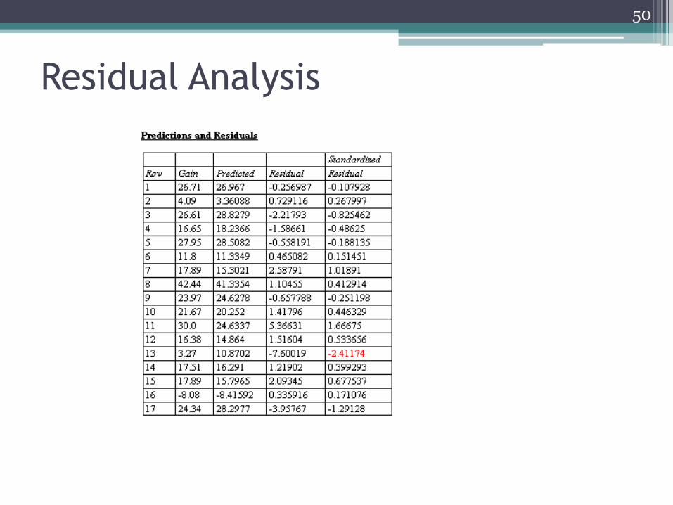
Residual Analysis

50

More Information

51

Statgraphics Centurion: www.statgraphics.com Uniwin Plus: www.statgraphics.fr or www.sigmaplus.fr Or send e-mail to info@statgraphics.com

Join the Statgraphics Community on:

Follow us on

52