Embed Size (px)
Citation preview

Page 1/20
Urban Greenness and Pricing Premium on Residential PropertiesAbdul Wahid
National University of Modern LanguagesMuhammad Zubair Mumtaz
National University of Science and Technology (NUST)Oskar Kowalewski ( [email protected] )
Polish Academy of Sciences
Research Article
Keywords: Urban Greenness, Pricing Premium, Machine Learning
Posted Date: June 1st, 2022
DOI: https://doi.org/10.21203/rs.3.rs-1691478/v1
License: This work is licensed under a Creative Commons Attribution 4.0 International License. Read Full License
Page 2/20
AbstractThis study examines how the urban climate affects the price, and urban greenness causes the pricing premium. To explore the greenness aspects, weconstruct a composite pollution index for each property traded in twin cities—Islamabad and Rawalpindi—based on the area traded properties' water, air, noise,and soil pollution. To examine the pricing e�ciency of these properties, we categorize our sample into green and non-green properties using machine learningand measure the impact of environmental factors on their price. Along with other property characteristics, we observe that air pollution, noise pollution, andwater pollution emerge as vital factors that de�ne the prices of properties. Similarly, investors are willing to pay higher prices for green residential propertieswith a lower pollution index. The study �ndings are helpful for investors, housing society managers and developers, as they show that greenness pays back.
JEL Codes: R20, R30, R31
1. IntroductionUrban climate has become a global challenge for residential areas and shifted the attention of policymakers, regulatory bodies, and housing authorities tominimize pollution by developing green infrastructure, ensuring compliance with urban environmental policies and minimizing carbon emissions. Creatingurban green amenities and green buildings provides a conducive living environment and further has important connections with the urban ecology (Francoand Macdonald 2018). Lambourne (2021) identi�ed that green buildings and infrastructure bring premium and pricing advantages for investors but the lackof relevant technical skills and apparent green buildings lead to investor disinterest. Although green building infrastructure is environment-friendly and canimprove consumers' social values, material costs, construction and transportation for green materials and green building features are more expensive thanconventional buildings in developing countries (Tam, Hao, and Zeng 2012). One argument is to create green buildings and another is to develop green spacesand parks to mitigate the warming and environmental dynamics. We can infer that properties located in green areas face low temperature and least humidityproblems, which cause the least energy consumption because more than one-third of the electricity generated in the world is being consumed in the residentialsector worldwide (Umbark, Alghoul, and Dekam 2020). Another counter argument is that the development of greenbelts, parks and green spaces in residentialareas is based on implementing environmental protection measures and increasing the cost of these residential properties. There is extensive empirical workon urban greenness (Franco and Macdonald 2018; Wang et al. 2013), green infrastructure and buildings (Chegut, Eichholtz, and Kok 2014; Low, Gao, and Teo2016), and the impact of greenness and green infrastructure on the �nancial performance and value of stock and portfolio allocation in Real EstateInvestment Trusts (Bhuyan et al. 2014; Coën and Des�eurs 2022; Ho (David), Rengarajan, and Lum 2013; Morri, Anconetani, and Benfari 2020). There is littlediscussion on urban climate dynamics and urban greenness on the value of residential real estate properties. Moreover, previous research on the amenityeffects of open space on the real estate market has typically used to capture the distance effects of different categories of greenness and green spaces on thevalue of properties.
Cho et al. (2008) highlighted that having higher greenness in residential areas to higher satisfaction among inhabitants of that speci�c area, which furtherleads to higher prices and rent prices. According to the Federal Board of Revenue report, properties located in Islamabad where greenness and climatedynamics are sound are priced higher than in Rawalpindi where the urban climate is poor (Federal Board of Revenue Pakistan 2019). This is the outcome ofthe information cascade which states that prices are moved by the number of people who make the same decision at the same time (Bartke and Schwarze2021; Xiao 2021); for example, buying and selling real estate properties sequentially due to successful information passing on (Salter and King 2009). Twofactors inculcate the information cascade i.e. (a) most investors are ex-patriates and they invest in real estate market sequentially (Wahid, Kowalewski, andMantell 2022). It is also evident that the Pakistanis diaspora sends huge amounts of money to Pakistan. According to the State Bank, Pakistan received arecord $21.84 billion in remittances in 2019-20 and 50% of this amount is invested in the real estate (Atiq 2020). Secondly, they observe the choices made bythose who invested earlier, and (b) they have some information aside from their own that helps guide their decision. The information they have beeninculcated by their earlier ex-patriate investors (Yousaf and Ali 2020).
The quality of green areas and parks (38.89 and 78.08) and dissatisfaction with green areas and parks (61.11 and 21.96) in twin cities-Rawalpindi andIslamabad are reported, respectively (Numbeo 2021) which further fuel that residents of Islamabad have a higher green living standard and higher quality ofgreenbelts and parks than residents of Rawalpindi do (Wahid et al. 2022). As the level of greenness and availability of quality greenbelts and parks increasewhich causes soundness in urban climate, ceteris paribus, the demand for residential properties will likewise increase. To the extent that demand increases,again, ceteris paribus, one would expect to observe an increase in prices and premiums on residential real estate. In this study, our focal point is to measurethe impact of urban climate dynamics on the prices of residential real estate properties. Secondly, to measure the role of greenness and climate indicators onthe pricing premium of properties.
To identify greenness, we construct an urban climate index for each property traded in twin cities—Islamabad and Rawalpindi—based on the water, air, noiseand soil pollution of the area traded properties. Furthermore, this study proposes three research questions: (a) How can one characterize the pricing of realestate property based on urban greenness? (b) What environmental factors in�uence the pricing of real estate properties of similar characteristics? (c) Howdoes the greenness of a residential area affect the value of real estate resulting in pricing advantages?
The rest of the paper is structured as follows. Section 2 presents a brief overview of the relevant literature and the research questions. Section 3 discusses ourdata and methodology, while Section 4 presents the results. Section 5 concludes.
2. Literature Review
2.1 Climate Dynamics and the Value of Real Estate

Page 3/20
In previous literature, various studies have been conducted on the connection between the value of real estate property and environmental aspects.Environmental factors, including the proximity of green belts and industrial zones, and the degree of air, noise and water pollution, play signi�cant roles inde�ning the prices of real estate properties. For instance, Rauf & Weber (2020) found that the hedonic pricing model re�ects the nominal effects ofenvironmental factors that cause variation in the pricing of real estate properties and assets. They also found that higher greenness of real estate leads tohigher prices. Similarly, Harrison et al. (2001) argued that environmental hazards have a signi�cant role in causing price distress and causing decreases in theprices of real estate properties. Current prices of real estate properties vary because of future disaster risks in nearby areas. The same evidence was alsoreported in England: the higher the probability of �ood and disaster risk, the higher the chances of devaluation of real estate properties. They also found thathouses and residential apartments were devalued up to 40% because of the continuous �ood events faced by areas nearest to a river (Lamond, Proverbs, andHammond 2010).
Troy & Romm (2004) and Ismail et al. (2016) also reported the same occurrence in California and Malaysia, respectively: the selling price of housing unitsdropped by 5% because the areas were suffering from �oods and the demand for properties in these areas also declined. J. Kim et al. (2017) also conducted astudy on natural disasters, i.e., �ooding and land sliding in Korea. The frequent disasters negatively affected residential real estate prices. The real estateproperties located approximately 1 kilometer from affected areas were found to have higher prices than those within 1 kilometer. Furthermore, their �ndingssuggest that new residential real estate societies must be developed in areas away from the disaster area. Floods and natural disasters are not the onlyfactors that lead to a variation in real estate prices, but the risk of wild�res also leads to variation. Stetler et al. (2010) identi�ed that in Montana, USA, theprices of and demand for real estate properties declined because of the risk of wild�res. However, many residents migrated from the affected area to non-affected areas of the country. The average selling price of housing units and apartments in the affected area declined because of the constant wild�re risk.Bin & Polasky (2004) found that in North California, millions of residents moved to other areas because of �oods and other natural disasters. The demand forresidential properties declined, and prices also decreased dramatically. Belanger & Bourdeau-Brien (2018) identi�ed that the overall worth of residentialproperties declines because of �oods and landslides in England. Therefore, English residents avoid investing in areas near the banks of rivers. Harrison et al.(2001) highlighted the same phenomenon of �ooding driving real estate property prices down in Alaska, USA. They found that the average selling price of thereal estate properties in �ood zones was recorded as lower than in other areas away from �ood zones.
2.2 Greenness of Residential Areas and the Value of Real EstateAs the distance increases from such natural sites, the average price of real estate properties decreases. On the other hand, the greenness of residential areasand the presence of green belts in nearby areas causes an increase in the prices of real estate properties with other physical attributes, such as the number ofbedrooms, kitchens, and the presence of many real estate properties in China (Jim and Chen 2006). Chiarazzo et al. (2014) also reported that the overall valueof real estate properties is more signi�cant in areas situated away from industrial areas in Spain. However, due to their low proximity to industrial areas, whichleads to less air and noise pollution, there is often an overvaluation of these real estate prices. Cho et al. (2008) concluded that in the United States of America,the preference for urban residences was greatly in�uenced by the availability of landscapes, green belts and rivers. Therefore, the pricing trend of apartmentswas found to be higher than the properties located near the green belt.
On the one hand, the greenness of residential areas and green buildings lower the probability of increasing global warming and natural disasters and higherconstruction costs due to the required environmentally friendly technology and measures. Juan et al. (2017) also highlighted that green buildings areexpensive compared to traditional buildings in China. They used an arti�cial neutral network model and concluded that green buildings signi�cantly positivelyimpact the environment. Similarly, Tam et al. (2012) found that green building implementation is environmentally friendly but is expensive compared to thetraditional construction of buildings in Hong Kong. The adoption of green building techniques could alleviate local industry issues. However, Ali & Al Nsairat(2009) used a green building assessment tool to determine the impact of green building on sustainability. They concluded that constructing green buildings inJordan is too expensive to be sustainable, but that the payoff of such a scheme would have a positive impact on the environment. According to Shan &Hwang (2018), many countries use a green building rating system to analyze the overall rating of green buildings. Adopting green real estate is worthwhile forstates that aim to minimize environmental hurdles. The outcome of green building development has a long-term impact on environmental stability in areaswhere the trend of green buildings is common.
2.3 Environmental Pollution and the Value of Real EstateLast but not least, a crucial aspect of the real estate market that has a signi�cant impact on the prices of real estate properties is reviewed. Cohen & Coughlin(2008) found the same pattern that was described above in Atlanta, in which housing prices decreased because of the presence of airports in nearby areas,which both cause noise pollution and disturb nearby residents; real estate properties located farther away from airports have a higher worth compared toproperties nearer to airports. Fan et al. (2021) also highlighted that the noise pollution caused by bus transit in Singapore has a similar effect on residents.Furthermore, they added that the purchasing trends of Singapore citizens near the most noise-affected areas were changed, as citizens preferred to invest inproperties in areas that were farther away from train and bus transit routes.
The same issues were highlighted in Taiwan by Liou et al. (2019), who found that the value of residential real estate properties declined because of the heavy�ow of tra�c. They further added that real estate prices were also affected by underground contaminated water. The average selling price of such real estateproperties decreased by 28% compared to those in the other areas of the city. Kim et al. (2010) conducted a study using a spatial lag hedonic model todetermine the impact of air pollution on real estate properties in Seoul, South Korea. They concluded that sulfur dioxide has a signi�cant effect on the pricesof residential areas. In contrast, the presence of nitrogen oxide had a negative association with the overall cost of residential real estate properties.
Likewise, Liu et al. (2017) also used a hedonic model and concluded that due to the poor water quality in Narragansett Bay, the overall prices of real estate arelower in coastal areas. They further concluded that the price of real estate properties is higher where better environmental conditions and basic utilities, suchas access to water, good air quality and low pollution, are present. Schläpfer et al. (2015) found the same pattern in Switzerland: pollution hurts the price of
Page 4/20
real estate properties. Housing units located closest to the green landscape areas were recorded to be higher in price. However, Önder et al. (2004) found thatthe average price of real estate in Istanbul declined because of poor soil conditions in similar areas. They also found no impact of earthquakes on residentialreal estate prices, but misinformation and speculation contributed to a decline in housing prices.
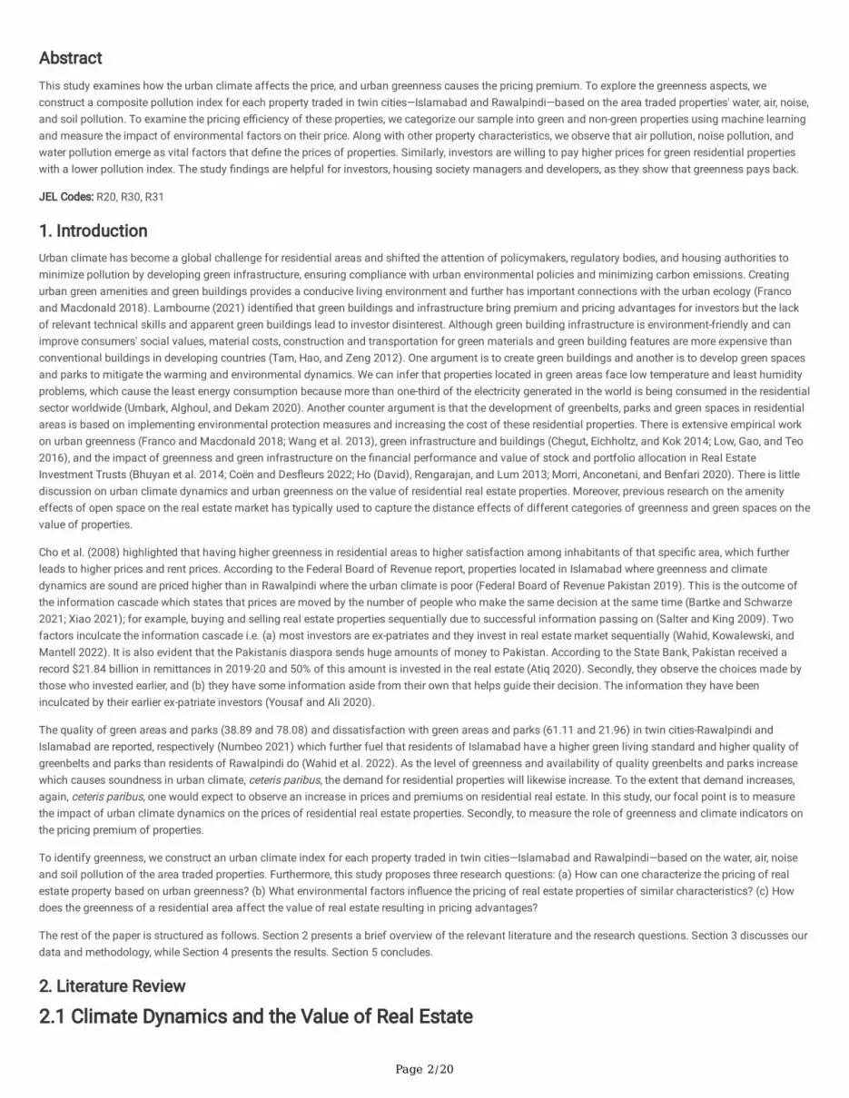
2.4 Environmental Dynamics of the Real Estate Market of PakistanPakistan spends approximately $5.2 billion on its housing market. This value constitutes approximately 2% of its GDP. The country is experiencing an averageannual growth rate of roughly 9% (Wahid, Mantell, and Mumtaz 2021). Pakistan’s high in�ation seems to have caused housing prices to increase sharply.Nationwide housing prices, in nominal terms, rose by 5.05% to PKR 10,875 (77 USD) per square foot (sq. ft). According to the Federal Board of Revenue (FBR),industry surveys estimate that the real estate industry was valued at approximately 700 billion rupees in 2015 (The News 2015). This estimation indicates thevalue of the real estate market since it has become Pakistan’s largest market. However, Pakistan’s real estate market is fragile due to environmental andnatural concerns. Table 1 shows that only the residential market of Islamabad is at an acceptable level in terms of the air, noise and water quality index, with73, 47.2 and 51.33 indices, respectively, which are all at moderate to good levels. Residents of other small and large cities of Pakistan are suffering fromsevere issues and pollution due to urban sprawl without proper environmental planning or conciseness.
Table 1Environmental Quality of Housing Markets of Pakistan
City Air Quality Index (µg/m3) Noise quality index (DB) Water quality index (Mg/l)
Islamabad 73 47.2 51.33
Lahore 76.59 64.51 75.52
D.G Khan 142 78.34 73.64
Rawalpindi 74 63.54 79.35
Multan 88 59 65
Quetta 77.5 68.06 83.82
Sukhur 151 83.23 75.24
Peshawar 159 54.69 55.47
Hyderabad 155 42.31 59.09
Nawabshah 147 71.32 72.92
Sialkot 108 56 67.71
Rahim Yar Khan 147 69.65 63.98
Sargodha 97 56.25 37.5
Karachi 157 69.47 82.94
Note: This table indicates the environmental dynamics of Pakistan. µg/m3, DB and Mg/l are denoted as micrograms per cubic meter, decibels, andmilligrams per letter, respectively. Source:(https://www.numbeo.com/pollution and https://www.iqair.com)
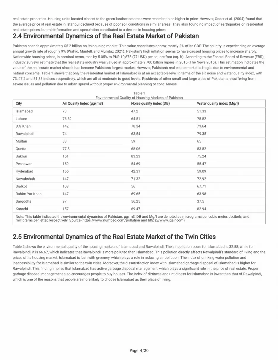
2.5 Environmental Dynamics of the Real Estate Market of the Twin CitiesTable 2 shows the environmental quality of the housing markets of Islamabad and Rawalpindi. The air pollution score for Islamabad is 32.58, while forRawalpindi, it is 66.67, which indicates that Rawalpindi is more polluted than Islamabad. This pollution directly affects Rawalpindi’s standard of living and theprices of its housing market. Islamabad is lush with greenery, which plays a role in reducing air pollution. The index of drinking water pollution andinaccessibility for Islamabad is similar to the twin cities. Moreover, the dissatisfaction index with Islamabad garbage disposal of Islamabad is higher forRawalpindi. This �nding implies that Islamabad has active garbage disposal management, which plays a signi�cant role in the price of real estate. Propergarbage disposal management also encourages people to buy houses. The index of dirtiness and untidiness for Islamabad is lower than that of Rawalpindi,which is one of the reasons that people are more likely to choose Islamabad as their place of living.
Page 5/20
Table 2Environmental Quality of the Housing Markets of Islamabad Rawalpindi
Indicators Islamabad Rawalpindi
Index Remarks Index Remarks
Air Pollution 32.58 Low 66.67 High
Drinking Water Pollution and Inaccessibility 41.95 Moderate 54.63 Moderate
Dissatisfaction with Garbage Disposal 36.16 Low 68.52 High
Dirty and Untidy 28.85 Low 65.74 High
Noise and Light Pollution 47.2 Moderate 63.54 High
Water Pollution 51.33 Moderate 79.35 High
Dissatisfaction to Spend Time in the City 29.06 Low 61.21 High
Dissatisfaction with Green and Parks in City 21.96 Low 61.11 High
Air quality 67.42 High 33.33 Low
Drinking Water Quality and Accessibility 58.05 Moderate 45.37 Moderate
Garbage Disposal Satisfaction 63.84 High 31.48 Low
Clean and Tidy 71.15 High 34.26 Low
Quiet and No Problem with Night Lights 52.8 Moderate 36.46 Low
Water Quality 48.67 Moderate 20.65 Low
Comfortable to Spend Time in the City 70.94 High 38.79 Low
Quality of Green and Parks 78.08 High 38.89 Low
Note: Table indicates the environmental dynamics of twin cities including air, noise, soil pollution index which further fuel dissatisfaction in residents oftwin cities. Sam is reported in above table. Source: (https://www.numbeo.com/pollution)
Similarly, Table 2 shows that Islamabad's noise and light pollution index is lower than that for Rawalpindi. The water pollution index for Islamabad is 51.33,while for Rawalpindi, it is 79.35, which is alarming for both twin cities because water pollution can lead to a vast variety of diseases. Generally, Pakistanremains exceptionally vulnerable to the impacts of climate change. According to the Global Climate Risk Index 2020, Pakistan is ranked �fth among thecountries most vulnerable to climate change. Between 1999 and 2018, the country witnessed 152 extreme weather events and suffered huge losses equaling$3.8 billion (UNDP 2020).
Furthermore, the dissatisfaction with time spent in the city of Islamabad is lower than in Rawalpindi, which indicates that people in Rawalpindi do not enjoyliving in it. Life in Islamabad is far better than that in Rawalpindi, which is why more people like to live in the city of Islamabad. Because of dissatisfactionwith greenery and parks, air quality, drinking water quality, and garbage disposal, satisfaction is higher among people in Islamabad, as shown in Table 2.People in Islamabad are more satis�ed with the city’s garbage disposal than in Rawalpindi, and this satisfaction also leads to a higher value of properties inIslamabad.
In addition, citizens’ satisfaction with other elements, such as cleanliness and tidiness, low noise pollution,, good water quality, comfort with spending time inthe city, and the quality of greenery and parks, Islamabad is much higher than in Rawalpindi, as shown in Table 2. The Capital Development Authority (CDA) inIslamabad has been actively involved in establishing new parks and maintaining existing parks. All of these values directly affect citizens' choices and theprices of properties. Islamabad has more facilities, which is one of the reasons that the real estate market value of Islamabad is higher than that ofRawalpindi. A survey conducted by the CDA revealed that 60% of respondents were happy with the elements mentioned in the questionnaire concerning theupkeep of green areas and plant care in Islamabad, and a total of 60% of individuals were pleased with the CDA’s efforts to halt the occupancy andencroachment on government property. Similarly, 60% were pleased with repairing sidewalks and lane markings, and 45% said they were satis�ed with thetimely collection and disposal of waste (Capital Development Authority 2021). These positive sentiments toward Islamabad’s real estate market lead to anincrease in the value of properties.
2.6 Pollution and Climate Dynamics in the Twin CitiesTable 3 compares air and noise pollution between the twin cities, i.e., Islamabad and Rawalpindi. The tra�c conditions in Islamabad are better than those inRawalpindi. Due to the highly populated area, there is an increase in tra�c �ow in Rawalpindi, and it has become more di�cult to travel within the city.According to a comparative review of the 2017 and 2021 surveys, tra�c on the major roads of Rawalpindi has increased threefold. According to the 2017survey, 75,000 and 275,000 vehicles passed through Ammar Chowk and Muree Road daily, respectively, while 300,000 and 600,000 vehicles passed throughAmmar Chowk and Muree Road daily in 2021 (tribune 2021). As a result, the time index, Exp. Index and ine�ciency index for Islamabad are better than thosefor Rawalpindi, as shown in Table 3.

Page 6/20
Table 3Air and Nosie Pollution in Islamabad Rawalpindi
Indicator Rawalpindi Islamabad
Tra�c Index: 199.77 157.75
Time Index (in minutes): 46.05 35.05
Time Exp. Index: 3997.14 565.11
Ine�ciency Index: 196.2 209.93
CO2 Emission Index: 5851.09 7129.33
Pollution Index: 76.96 41.86
Pollution Exp Scale: 135.6 70.55
PM10 448 217
PM2.5 107 66
PM10 Pollution Level: Extremely High Extremely High
Note: Table indicates the magnitude of noise pollution due to tra�c and air pollution due to carbon emission produced by tra�c. PM10 indicates PM10describes inhalable particles with diameters generally 10 micrometers and smaller. PM 2. 5 refers to the atmospheric particulate matter with a diameter ofless than 2.5 micrometers, which is about 3% of the diameter of human hair. Source: (https://www.numbeo.com)
Furthermore, the pollution index, the index of pollution exp. scale and other indices such as PM 10, PM 2.5 and the index of PM10 pollution level in Islamabadare environmentally sound and lower than those in Rawalpindi. These indices show that pollution in Islamabad is lower, therefore, more people want a houseand to live in Islamabad which results in higher prices of real estate property. The greater the demand is, the higher the price will be. The values of theseindices have a signi�cant impact on the real estate market prices. Comparatively, the indices of Islamabad are better, which directly affects the price ofproperty. Owing to these values, the price of a house in Islamabad is almost double that of a house in Rawalpindi. The demand and price are both higher inIslamabad than in Rawalpindi. Demand drives sales, and demand continues to climb. The population of Islamabad has not decreased, which explains why thehousing demand continues to rise year after year. Aside from the bleak and tragic views of recent years, there is reason to believe that the real estate market inIslamabad will have a lot to look forward to in 2021. This lovely and rich city is known for its pleasant weather (dawn 2021).
Table 3
Regarding environmental factors, all indicators, such as proximity to industrial zones, proximity to green belts, air pollution, noise pollution, and probability ofdisaster, signi�cantly impact pricing. Generally, Pakistan’s environmental conditions have been gradually worsening. Lahore has become the 2nd highestpolluted city in the world. Rawalpindi had a PM2.5 average of 40.8 µg/m³, placing it into the ‘unhealthy for sensitive groups’ bracket, which requires a PM2.5reading of anywhere between 35.5 to 55.4 µg/m³ for classi�cation. This reading places Rawalpindi at 8th place out of all cities registered in Pakistan and224th place in all cities ranked worldwide in terms of their pollution levels. The climate dynamics of Rawalpindi are very sound, as shown in Fig. 1.
Figure 1
Islamabad is making gradual improvements to its air quality. In 2017, Islamabad had a PM2.5 yearly average of 39.2 µg/m³, placing it into the ‘unhealthy forsensitive groups’ bracket (35.5 to 55.4 µg/m³). The climate dynamics of Islamabad are very sound, as shown in Fig. 2.
Figure 2
3. Methodology
3.1 Data and SourcesWe collected data on 1580 properties located in Islamabad and Rawalpindi. After removing the outliers and missing values, our sample was reduced to 1500properties. Of this, 48% of the data came from Islamabad and 52% related to Rawalpindi. The market value of properties was obtained from Zameen.com,OLX, property dealers, local housing authorities, and other property recording systems in Islamabad and Rawalpindi. The data include 10% of the overalltraded properties in Islamabad and Rawalpindi from 2017 to 2019 before covid-19 pandemic. To match the prices and characteristics of the properties, weidenti�ed the location and local housing authority of the property from its sale agreement. To measure the property’s proximity to essential utilities such asschools, hospitals, railway stations, airports, consumer markets, and megaprojects, we used Google Maps. The market sentiment at the date of sale of aspeci�c property was calculated using data provided in the economic survey of Pakistan in the construction and real estate sectors.
3.2 Hedonic Model with GreennessTo examine the determinants of the pricing of real estate properties in Pakistan, we applied the hedonic regression method along with environmental factorsto capture the impact of the greenness of residential areas on the value of real estate properties.
Price = f (location, structure, neighborhood, and environmental factors) (1)

Page 7/20
Equation (1) explains that the price of real estate depends on its characteristics (e.g., location, structure, neighborhood, environmental, and administrativefactors). Consequently, we develop the following model:
Pricei = αi + δi ProxRail + Proxairp + δi ProxCCen + γi NoBedr + γi NoBatr + γi SizeBedr + γi AvaiGar + γi AvailGarg + γ
2
where prices indicate the total price of the house. The �rst three indicators of proximity to railway stations, airports, and city centers depict the role of locationin the pricing of real estate property in Pakistan. These are further elaborated on: Prox-Bus represents the geographic proximity of each speci�c property to ametro bus station, Prox-Rail indicates the geographic proximity of each speci�c property to a railway station, Prox-air exhibits the geographic proximity of eachspeci�c property to an airport, and Prox-ccen indicates the geographic proximity of each speci�c property to the city centers of both cities—the Blue Area inIslamabad and Saddar Bazar in Rawalpindi.
Furthermore, �ve features, such as the number of bedrooms, bathrooms, size of the rooms, presence of gardens, and garages, depict the structure of houses. NoBedrandNoBatr depict the total number of bedrooms and bathrooms, respectively. Similarly, SizeBedr indicates the size of each room, and AvaiGar and AvailGarg indicate the availability of a garden and garage, respectively. Additionally, the role of the property’s neighborhood is also considered in this study;for example, ProxMkt, ProxSch, and ProxJob indicate the geographic proximity of each speci�c property to market, school, and job centers, respectively, and Crimerate depicts the total number of criminal cases reported at the nearest police station.
Pollu-water indicates underground water quality, and Prox-indus re�ects the proximity of selected residential areas from industrial zones. Similarly, prox-greenbelt indicates the geographical distance from green belts, and air pollut and noise pollution re�ect selected sample areas' air pollution and noisepollution index. Disrisk indicates the proximity of real estate residential areas from disaster or �ood zones, e.g., Nala Lai in Rawalpindi and the probability ofearth quickly.
Furthermore, to clarify the model’s speci�cation and robustness of the variables, we use LASSO regression, which is widely used to select variables andmeasure the model's accuracy. This technique was �rst introduced by Santosa and Symes (1986) and used by Tibshirani (1996). The speci�cations of theLASSO regression are as follows:
Pricei =1
2m
m
∑i=1
yi − β0 +p
∑j=1
xiβj
2+ λ
p
∑j=1
βj
(3)
To estimate the boundary of the fair price, we use stochastic frontier analysis (SFA) by using the following equation:
{Price}_{i}=f\left({x}_{i}, \beta \right)+{ϵ}_{i}
(4)
{ϵ}_{i}={v}_{i}-{u}_{i}5
where the subscript i indicates the number of cross-sections or observations—1500 in our case. {Price}_{i} indicates the fair offer price, and {x}_{i} denotes thejx1 vector of determinants identi�ed in Eq. (1) after removing the fragile characteristics. {u}_{i} is the log difference between the fair price and actual offer price({u}_{i}={ln fair price}_{i}-{ln actual price}_{i}). By rearranging the equation, we obtain \text{exp}\left(-{u}_{i}\right)=\frac{actual price}{Fair price}. We apply theSFA to measure the pricing ine�ciency of real estate properties of different housing societies in Islamabad and Rawalpindi using cross-sectional data. Thismeasure is based on observations across low- and high-prestige societies. We used an output-oriented model that estimates the output technical e�ciencyusing input or factors determining the price, for example, in our case, the different features of houses (e.g., structure, location, and neighborhood) to calculatethe maximum level of price denoted as the “fair price” in our study.
3.3 Arti�cial Intelligence (AI)We applied machine learning on 1500 observations, including 1046 (69.7%) observations and 454 (30.3%) were holdout and test with trained data. Allcharacteristics of hedonic model were taken as control variables and water, air, noise and soil pollution were tested. The train set was used to train AI/machinelearning (ML) techniques, and the test set evaluated the AI/ML techniques. We applied Support Vector Machine (SVM), Stochastic Frontier Analysis (SFA),OLS, LASSO, Logistic Regression (LR), Decision Tree (DT), Random Forest (RF), and Arti�cial Neural Networks (ANNs) using the AI/ML libraries of Python.SVM was applied to classify the binary decision, which constructs a hyperplane(s) in a high-dimensional space that maximizes the margin. The large marginmeans a lower generalization error and better performance; it usually performs well on a complex and nonlinear but medium-sized dataset (Cortes and Vanik1995).
4. Findings And Discussion
4.1 Determinants of Prices of Real Estate
( ) ( ) ( ) ( ) ( ) ( ) ( ) ( )
( ) | |

Page 8/20
To test the hedonic model's impact and sensitivity on residential properties' prices along with environmental factors, we used Model 1, which shows theimpact of the hedonic model on the price of residential properties in Islamabad and Rawalpindi. Table 4 shows that the house size, number of bedrooms, andpresence of gardens (\beta=2.254, 0.465 & 2.838, p < 0.05) have signi�cant positive impacts on the prices of residential real estate properties, which showsthat the design of real estate property has a strong and positive impact on the prices of residential properties. Similarly, the proximity to the nearest markets,proximity to city centers and crime rate (\beta= -0.582, -0.009 and − 0.057 p < 0.05, respectively) have a signi�cant positive impact on the prices of residentialreal estate properties. In this model, house size and crime rate are very prominent factors explaining the variation in the prices of real estate properties inPakistan. The crime rate is an external factor that affects the overall region and sector prices if the crime rate is higher than the average crime reported in anycity or country. According to the latest stats released by the World Crime Index issued in a report by the international organization Numbeo, Islamabad’s currentsafety index stands at 71.37, which is remarkable if we compare it with Rawalpindi, which stands at 67.12. Because of Islamabad’s low crime rates, the UnitedNations (UN) also restored Islamabad’s status as a family station. This status means that the UN's International Civil Service Commission (ICSC) considersIslamabad a safe city for UN personnel to visit with their families. As a result, the prices of residential properties in Islamabad are higher than those inRawalpindi.

Page 9/20
Table 4Determinants of Prices of Real Estate Properties
Model-I Model-II Model-III Model-IV Model-V Model-VI Model-VII LASSO
HouseSize
2.254 2.256 2.258 2.259 2.255 2.247 2.240 2.008
(20.33)** (20.37)** (20.39)** (20.38)** (20.36)** (20.30)** (20.15)** (37.82)**
No.Bedrooms
0.465 0.462 0.465 0.466 0.472 0.468 0.464 0.004
(2.42)* (2.41)* (2.42)* (2.43)* (2.46)* (2.45)* (2.42)* (2.46)**
Room Size 0.002
(0.62)
No.Bathrooms
0.162
(0.72)
Presenceof Garden
2.838 2.821 2.803 2.809 2.743 2.747 2.757 3.153
(2.34)* (2.33)* (2.31)* (2.31)* (2.26)* (2.27)* (2.28)* (3.24)**
Presenceof Garage
0.047
(0.04)
ProxRailwayStation
0.008
(0.23)
ProxMarket
-0.582 -0.568 -0.570 -0.571 -0.596 -0.588 -0.581 -0.639
(3.53)** (3.45)** (3.47)** (3.47)** (3.62)** (3.57)** (3.52)** (4.01)**
Prox Citycenter
-0.009
(2.18)*
ProxAirport
-0.055
(1.85)
ProxSchool
-0.152
(0.99)
Prox JobPlaces
-0.129 -0.126 -0.130 -0.134 -0.106 -0.123 -0.115 -0.193
(2.83)** (2.77)** (2.85)** (2.84)** (2.19)* (2.50)* (2.26)* (2.00)*
Crime rate -0.057 -0.053 -0.052 -0.048 -0.040 -0.033 -0.037 -0.040
(3.48)** (3.23)** (3.16)** (2.52)* (2.06)* (1.67) (1.80) (2.35)*
WaterPollution
-2.202 -1.823 -1.894 -1.502 -1.230 -0.324
(2.03)* (3.49)** (4.53)** (4.30)** (4.14)** (0.19)
GreenIndex
-2.309 -2.202 -2.455 -2.618 -2.516 -1.948
(4.09)** (5.03)** (5.15)** (5.22)** (5.17)** (3.80)**
ProxGreenbelt
0.013 0.012 0.017 0.013 0.022
(5.33)** (5.05)** (5.19)** (4.08)** (5.05)**
Note: The study sample comprises 1500 property situations in Rawalpindi and Islamabad. Akaike’s Information Criterion (AIC), Bayesian Information Criterion(BIC). ***; ** represent signi�cance at the 1% and 5% levels, respectively.

Page 10/20
Model-I Model-II Model-III Model-IV Model-V Model-VI Model-VII LASSO
AirPollution
-0.069 -0.042 -0.036 -0.070
(4.20)** (5.26)** (3.04)** (2.35)*
NoisePollution
-0.066 -0.066 -1.891
(4.13)** (2.10)* (4.22)**
SoilPollution
-0.030 -0.121
(3.67)** (5.12)**
Cons 0.522 1.464 2.638 2.695 0.282 1.604 1.416 1.244
(0.22) (0.57) (0.94) (0.96) (0.09) (0.51) (0.44) (0.54)
R2 0.60 0.64 0.65 0.67 0.71 0.72 0.77 0.78
Df
AIC
BIC
13
5212.47
5309.99
14
4820.414871.21
15
4615.064672.08
16
4517.11
4579.32
17
4399.314367.59
18
4298.884272.84
19
4239.01
4218.03
Note: The study sample comprises 1500 property situations in Rawalpindi and Islamabad. Akaike’s Information Criterion (AIC), Bayesian Information Criterion(BIC). ***; ** represent signi�cance at the 1% and 5% levels, respectively.
Similarly, environmental factors have been tested to measure the impact of each variable on the prices of residential properties using a hedonic model.Environmental variables are added to the speci�cation incrementally from Model II to Model VIII. To test the robustness of the environmental control variables,we apply three criteria: Akaike’s information criterion (AIC), Bayesian information criterion (BIC) and {R}^{2}. In Model II, we added our variable representingwater pollution. The test statistics are AIC = 4820.41, BIC = 4871.21, and R2 = 0.64. The value of \beta = -2.202 for this variable is signi�cant at the 95%con�dence interval (p < 0.05). Thus, the explanatory power of this model is superior to that of Model-I, as signi�ed by a lower AIC and BIC and a higher R2.These �ndings indicate that groundwater availability is a crucial factor when explaining the prices of residential areas in Islamabad and Rawalpindi.According to the Water and Sanitation Agency (WASA), due to the high demand for water and low rainfall, the ground water level of the twin cities has droppedto 600 feet, which is worsened by the water level continuing to fall approximately 6 feet annually. However, according to some independent analysts, theannual groundwater level falls by seven to nine feet (Shirazi 2021). As a result, residents of the twin cities pay approximately Rs15000 to Rs17000 (100–110USD) for a tanker that contains 1000 to 1200 liters of water.
In Model III, we added a variable representing the proximity to industrial areas. The test statistics are AIC = 4615.06, BIC = 4672.08, and R2 = 0.65. The value of\beta =-2.309for this variable is signi�cant at the 99% con�dence interval (p < 0.01). The explanatory power of this model is superior to that of Model-I, assigni�ed by a lower AIC and BIC and a higher R2. In prior literature, researchers have also explored whether proximity to industrial areas causes variousenvironmental issues that further fuel the low prices of residential areas near these industrial zones (Perlin, Wong, and Sexton 2001). Similarly, we includedproximity to green belts and obtained AIC = 4517.11, BIC = 4579.32, R2 = 0.67. The value of \beta =0.013for that variable is signi�cant at the 99% con�denceinterval (p < 0.01) as shown in Table (4). Cho et al. (2008) identi�ed that investors prefer urban residences near landscapes, green belts and rivers. It isgenerally presumed that as proximity to greenbelts decreases, ceteris paribus, the demand for residential properties near greenbelts will likewise increase. Tothe extent that demand increases, again, ceteris paribus, one would expect to observe an increase in the prices of residential properties near green belts.
In Model V, we included air pollution as an environmental factor to measure the effects of air pollution on the prices of residential properties in Pakistan. Theresults show that due to the inclusion of air pollution, AIC = 4399.31, BIC = 4367.59, and R2 = 0.71. The value of \beta =-0.069for this variable is signi�cant atthe 99% con�dence interval (p < 0.01) as shown in Table 4. This value indicates that air pollution has a signi�cant role in de�ning the prices of real estateproperties in Pakistan. The air quality index of both Rawalpindi and Islamabad is declining annually, which poses a heavy threat to both the environment andhuman health. The trickle-down effects of air quality can be seen in Pakistan's residential properties' prices. Industrialization, unplanned urbanization, andhuge tra�c volumes contribute to air pollution. Looking at the statistics from 2019, Rawalpindi had a PM2.5 average of 40.8 µg/m³, placing it into the‘unhealthy for sensitive groups’ bracket, which requires a PM2.5 reading between 35.5 and 55.4 µg/m³ for classi�cation. This reading places Rawalpindi as8th out of all cities registered in Pakistan and 224th place in all cities ranked worldwide in terms of their pollution levels. On the �ip side, regarding the airpollution levels, Islamabad had PM2.5 readings of 35.2 µg/m³ as a yearly average in 2019. This average ranks it as the cleanest city in the country, at 10thplace out of all cities currently ranked in Pakistan.
Similarly, we test the potential impacts of noise pollution on the prices of residential properties in the twin cities. In this regard, we included noise pollution asan explanatory variable in the model, and the �ndings show that model VI, in which noise pollution is included, performed better in terms of AIC = 4298.88, BIC = 4272.84, and R2 = 0.72. The value of \beta = -0.066 for this variable is signi�cant at the 99% con�dence interval (p < 0.01). This value shows that noisepollution signi�cantly impacts the prices of residential properties in the twin cities. Similarly, disaster risk shows that the higher the risk of disaster is, the lowerthe prices of residential properties in the twin cities.

Page 11/20
4.2 Pricing Premium Based on GreennessTo test the greenness of real residential properties, we constructed an urban climate index for each selected property of our sample. This index included airpollution, noise pollution, water pollution, and soil pollution in the speci�c area where the traded property is located. The index is based on accuracy andprecision obtained using machine learning of air pollution, noise pollution, water pollution, and soil pollution, as shown below: -
{Evirenmenal Score}_{i}={Accuracy Level* water pollution index}_{i}+{ccuracy Level*air pollution index}_{i}+ {ccuracy Level*Noise pollution index}_{i}+ ccuracyLevel*{Soil pollution index}_{i} \left(6\right)
We calculated the environmental score of each speci�c property based on air pollution, noise pollution, water pollution and the soil pollution index. Based onenvironmental score, we calculate the greenness index of each property as follows: -
{\text{U}\text{r}\text{b}\text{a}\text{n} \text{C}\text{l}\text{i}\text{m}\text{a}\text{t}\text{e} Index}_{i}= \frac{({Evirenmenal Score}_{i}-Min.{EvirenmenalScore}_{j})}{(Max.{Evirenmenal Score}_{j}-Min.{Evirenmenal Score}_{j})}7
{Evirenmenal Score}_{i} indicates the environmental score of each property, Min.{Evirenmenal Score}_{j} \& Max.{Evirenmenal Score}_{j} indicate the minimumand maximum score of the entire sample.
Furthermore, we also calculated the median index. If the score of a speci�c property is equal to or higher than the median of urban climate index, it wascategorized as non-green; otherwise, it was categorized as a green residential property. Further, to validate our calculation of the dummy based on theenvironmental score, we use ML in Python. The result of the ML model as shown in Table 5 indicates accuracy above 80% and that the SVM, LR, DT, RF, andANN models were deployed correctly. The comparison of the different ANN architectures is also shown Fig. 3. Therefore, we can assume that theseenvironmental indicators accurately measure the greenness of residential areas.
Table 5
Accuracy and Con�rmatory Diagnostics for Greenness Using MLMethod Accuracy Precision Recall F1 score
SVM (Linear) 0.771 0.825 0.833 0.761
SVM (RBF) 0.791 0.776 0.847 0.794
Logistic Regression 0.757 0.824 0.798 0.795
Decision Tree 0.766 0.805 0.802 0.771
Random Forest (Estimators = 3) 0.819 0.797 0.779 0.825
Random Forest (Estimators = 5) 0.823 0.765 0.813 0.767
Random Forest (Estimators = 8) 0.820 0.782 0.84 0.822
Random Forest (Estimators = 10) 0.844 0.852 0.791 0.782
Random Forest (Estimators = 15) 0.763 0.788 0.761 0.853
ANN (Layers = 2, Neurons = 64) 0.831 0.805 0.775 0.787
Note: The table indicates the accuracy of the measure for the segregation of housing societies into high prestige = 1 and low prestige = 0 based on socio-economic and environmental preferences, using Python and 1500 observations. SVM: support vector machine, LR: logistic regression, DT: decision tree,RF: random forest, ANN: arti�cial neural networks.
We used stochastic frontier analysis (SFA) to test the pricing e�ciency. Table 6 shows that green residential properties are overpriced by an average of 3.676million rupees (an average actual price = 30.3454, an average estimated fair price = 26.668), as shown in Fig. 4, and similarly, non-green residential real estateis underpriced by an average of -0.222 (an average actual price = 28.222, an average estimated fair price = 28.445), as shown in Fig. 5.

Page 12/20
Table 6Estimation of Fair Prices of Real Estate Properties
Green Residential Area Non-Green Residential Area
OLS SFA OLS SFA
House Size 2.145 2.162 3.180 3.180
(14.60)** (15.16)** (12.34)** (12.47)**
No. Bedrooms 0.345 0.340 2.509 2.509
(3.58)** (4.63)** (4.73)** (4.78)**
Room Size 0.001 0.001 0.028 0.028
(0.20) (0.24) (3.68)** (3.71)**
No. Bathrooms 0.321 0.241 0.185 0.185
(0.93) (0.70) (0.66) (0.66)
Presence of Garden 3.497 3.376 0.540 0.540
(2.28)* (2.27)* (0.21) (0.22)
Presence of Garage 1.406 1.464 0.985 0.984
(0.93) (1.00) (0.37) (0.38)
Prox Railway Station -0.183 -0.196 -0.193 -0.193
(1.20) (1.32) (4.89)** (4.94)**
Prox Market -0.909 -0.945 -0.246 -0.246
(3.41)** (3.61)** (1.26) (1.27)
Prox City center -0.050 -0.047 -0.114 -0.114
(3.60)** (5.57)** (1.70) (1.72)
Prox Airport -0.328 -0.332 -0.017 -0.017
(5.08)** (5.23)** (0.50) (0.51)
Prox School -0.496 -0.487 -0.443 -0.443
(2.23)* (2.23)* (2.15)* (2.17)*
Prox Job Places -0.039 -0.047 -0.258 -0.258
(0.60) (0.72) (3.99)** (4.03)**
Crime rate -0.189 -0.191 -0.141 -0.120
(4.04)** (4.01)** (5.01)** (5.01)**
Cons 6.446 4.420 4.303 4.209
(1.29) (1.39) (1.98) (1.97)*
R2 0.66 0.80
N 710 710 790 790
Actual Price 30.3454 28.222
Fair Price (26.668) (28.445)
Mean Difference 3.676** -0.222**
Note: This table displays the determinants of fair prices of a sample of 1500 real estate properties using SFA. Price of the properties are presented in PKRs(million). To test the signi�cant difference in the mean, a t-test was applied. ***; ** represent signi�cance at the 1% and 5% levels, respectively.
Rawalpindi and Islamabad are more than just the inseparable twins of Pakistan – one is the capital and home to highly esteemed bureaucrats, diplomats, andfamous personalities of Pakistan, while the other hosts the headquarters of the armed forces of the country. The debate over the superior twin – Rawalpindivs. Islamabad – has existed for a long time. The cost of living in both cities differs for several reasons. This trend shows that investors are willing to payhigher prices for increased greenness and puri�cation. The most crucial factor in Islamabad’s favor is that it is famous for featuring lavish lifestyles with ahigh cost of living. Rawalpindi is relatively economical, and it is cherished by anyone who is looking to make the most of a limited budget.

Page 13/20
4.3 Urban Greenness and Pricing AdvantagesIn order to test the effects of the urban greenness index and the individual environmental factors on the pricing dynamics of residential properties. We divideour sample into four quartiles and applied SFA on these four the models separately i.e. Model-I = urban pollution index < 25%, (b) Model-II = urban pollutionindex > 25% < 50%, (c) Model-III = urban pollution index > 50% % < 75% and (d) Model-IV = urban pollution index > 75%. The result in Table (7) Model-I to Model-IV shows that green residential properties to non-green properties are overpriced and underpriced by an average of (mean difference = 4.97**, 2.31**, -0.24**and − 3.76**) which teaches that the higher the level of urban greenness cause lower urban pollution index which further lead to pricing advantages forresidents of these areas. The interrelationship between urban pollution and pricing performance is also shown in Fig. 6. One of the reasons for the differencein prices of residential properties in Islamabad and Rawalpindi is the increased presence of greenbelts, parks and natural water resorts in Islamabad.Islamabad, situated at the foothills of Margalla, is known across the globe for its exceptional natural beauty, lush green landscapes and hiking trails, whichfurther fuel increases in the prices of real estate in the city.
Similarly, water pollution in the real estate market has signi�cant importance in determining the prices of residential properties. Lamond, Proverbs, andHammond (2010) found that houses and residential apartments were devalued by up to 40% because of water pollution. We include the water pollution indexin Model-V and �nd that properties are underpriced by -1.47** million due to water pollution as shown in Table (7), which shows that water pollution plays asigni�cant role in de�ning the pricing of residential properties in twin cities.
Kim et al. (2010) identi�ed that sulfur dioxide and nitrogen oxide signi�cantly impact residential areas. Although residential areas of Islamabad show betterperformance in air quality index compared to rest of the cities of Pakistan, Pakistan as a whole is generally suffering from air pollution, as Pakistan is rankedas the country with the 2nd highest air pollution on average, with a US Air Quality Index (AQI) score of 152 (Iqair.com 2021). To test the impact of air pollutionon real estate property prices, we included the air pollution as explanatory in Model-VI by controlling hedonic characteristics and we �nd that air pollutioncause underpricing by -2.19** million as shown in Table 7. This shows that higher the air pollution, the higher the pricing disadvantage.

Page 14/20
Table 7Estimation of Fair Prices of Real Estate Properties
Model-I Model-II Model-III Model-IV Model-V Model-VI Model-VII Model-VIII
House Size 1.955
(7.10)**
1.722
(4.50)**
1.264
(2.63)**
1.736
(6.33)**
1.058
(19.94)**
1.853
(19.16)**
1.872
(18.99)**
1.885
(19.02)**
No. Bedrooms 3.563
(4.01)**
2.977
(2.43)*
0.582
(3.28)**
0.496
(3.01)**
0.562
(3.35)**
0.537
(3.18)**
Room Size 0.055
(3.51)**
0.047
(2.26)*
0.038
(2.23)*
0.024
(2.23)*
0.067
(2.05)*
No. Bathrooms 1.263
(2.35)*
1.688
(2.26)*
Presence of Garden 3.241
(3.75)**
3.101
(3.00)**
Presence of Garage 1.101
(4.25)**
1.585
(4.34)**
1.454
(3.15)**
Prox Railway Station -0.039
(1.11)
-0.129
(2.21)*
-0.014
(3.58)**
Prox Market -0.353
(3.40)**
-0.166
(2.22)*
-0.193
(2.11)*
-0.456
(3.00)**
Prox City center -0.014
(1.13)
-0.011
(2.24)*
Prox Airport -1.241
(3.75)**
-2.101
(3.12)**
-1.241
(3.75)**
Prox School -1.561
(3.25)**
-1.585
(6.34)**
-1.098
(3.15)**
-1.089
(4.25)**
-1.651
(4.34)**
Prox Job Places -0.039
(1.11)
-0.129
(2.21)*
-0.014
(3.58)**
-0.039
(1.11)
Crime rate -0.353
(3.40)**
-0.166
(2.22)*
-0.193
(2.11)*
-0.456
(3.00)**
-0.353
(3.40)**
Usigma -3.241
(4.75)**
-0.183
(2.75)**
-0.196
(4.11)**
-0.193
(1.23)
-0.193
(1.56)
-0.196
(4.11)**
-1.321
(3.75)**
-3.110
(3.75)**
Water Pollution -0.481
(15.50)**
Air Pollution -0.349
(22.80)**
Noise Pollution -0.637
(21.13)**
Soil Pollution -0.743
(20.54)**
Avg. Actual Price 30.43 29.43 26.43 27.43 26.43 26.01 25.21 25.34
Avg. Fair Price 25.46 27.12 26.67 31.19 27.90 28.20 28.12 26.02
Mean Difference 4.97** 2.31** -0.24** -3.76** -1.47** -2.19** -2.91** -0.68
Note: Model-I = urban pollution index < 25%, (b) Model-II = urban pollution index > 25% < 50%, (c) Model-III = urban pollution index > 50% % < 75% and (d)Model-IV = urban pollution index > 75%. In Model V-VIII, water, air, noise and soil pollution are included as explanatory variables.

Page 15/20
Model-I Model-II Model-III Model-IV Model-V Model-VI Model-VII Model-VIII
Vsigma -1.123
(1.75)
-0.103
(1.02)
-0.121
(1.11)
-0.193
(1.23)
-0.211
(1.56)
-0.312
(1.11)
-1.810
(1.15)
-1.212
(1.21)
N 330 206 456 508 1,500 1,500 1,500 1,500
Note: Model-I = urban pollution index < 25%, (b) Model-II = urban pollution index > 25% < 50%, (c) Model-III = urban pollution index > 50% % < 75% and (d)Model-IV = urban pollution index > 75%. In Model V-VIII, water, air, noise and soil pollution are included as explanatory variables.
Fan et al. (2021) highlighted that noise pollution strongly in�uences on the prices of residential real estate. This pollution is an invisible danger that cannot beeasily observed but is present nonetheless. Noise pollution is considered to be any unwanted or disturbing sound that affects the health and well-being ofhumans and other organisms. There are various sources that cause noise pollution, including street tra�c, air tra�c, construction sites, catering and night life,and animals. To test the impact of air pollution on real estate property prices, we included noise pollution as an explanatory variable Model-VII by controllinghedonic characteristics and we �nd that noise pollution cause underpricing by -2.91** million. This shows that the higher the air pollution, the higher thepricing disadvantage. We �nd that soil pollution has no signi�cant impact on prices of residential real estate properties.
We also use the Machine Learning (ML) mechanism to measure the role of water, air, noise and soil pollution on overall sample. The out of 1500 observations,1046 (69.7%) observations were trained and 454 (30.3%) were holdout and test with trained data. The result of SVM: support vector machine, LR: logisticregression, DT: decision tree, RF: random forest, ANN: arti�cial neural networks showed 80–85% accuracy and precision. The result shown in Figure (7) showsthat having similar characteristics of properties, water, air and noise pollution play a signi�cant role in de�ning prices. The population of Islamabad isincreasing very quickly due to migrants from Afghanistan and other cities in Pakistan because of capital territory and employment opportunities. This alsoincreases various types of pollution, such as air, noise, and soil pollution. However, Islamabad has fared very well compared to its neighboring cities, free ofthe catastrophic spikes of pollution that some of them display. The Capital Development Authority (CDA) has implemented various initiatives to improve theenvironmental conditions in Islamabad, with a yearly average of 38.6 µg/m³. Due to these initiatives and the greenness of the residential areas of Islamabad,the prices of properties in Islamabad are higher than those in Rawalpindi.
5. ConclusionThe main goal of this paper is to measure the impact of the greenness of residential properties on their prices and determine how much more investors arewilling to pay for properties in green residential areas than those in non-green residential areas and greenness causes pricing advantages. We �nd that thehigher the level of greenness and the lower the pollution index, the more investors are willing to pay. Second, air pollution, noise pollution, water and soilpollution emerged as vital factors de�ning the prices of properties in the hedonic model. This result indicates that urban greenness as an output of urbanclimate has a signi�cant role in determining the pricing advantages.
The study's �ndings are different from previous literature that investors are willing to pay higher prices for the properties even those located very far from thecity center and job places due to greenness and low pollution index. There are two reasons for it, (a) most cities of Pakistan are highly polluted due to thehigher level of urban climate which in result causes various diseases, especially for children and old age family members and (b) after the Paris agreement,regulatory bodies are trying to encourage and ensure compliance with environmentally friendly initiatives which further leads to the development of newsocieties outside the cities with least urban climate risks and higher greenness. In addition, �nancial institutions are directed to pay mortgages to greenhousing societies and residential areas.
The �ndings of this study may be of interest for regulatory bodies and investors as it contributes to strategies for enhancing the value of their properties byfocusing on the environment. This study used only the different external characteristics of real estate properties. To build on these �ndings, future researchshould be conducted on how the greenness of residential areas and societies encourages expatriates to invest, which can further lead to higher FDI in�ows ofgreen properties and remittances, and how much an investor can earn from green properties in the long run by comparing the prices of green and non-greenproperties by holding for the short- and long-run.
DeclarationsFunding
The authors declare that no funds, grants, or other support were received during the preparation of this manuscript.
Competing Interests
The authors have no relevant �nancial or non-�nancial interests to disclose.

Page 16/20
Author Contributions
Abdul Wahid and Muhammad Zubair Mumtaz contributed to the study conception and design. Material preparation, data collection and analysis wereperformed by Abdul Wahid and Zubair Mumtaz. The �rst draft of the manuscript was written by Abdul Wahid and all authors commented on previous versionsof the manuscript. All authors read and approved the �nal manuscript.
References1. Ali, H. H., & Al Nsairat, S. F. (2009). Developing a green building assessment tool for developing countries–Case of Jordan. Building and environment,
44(5), 1053-1064.
2. Atiq, Syed Khurram. 2020. The Real Estate in Pakistan: Prospects and Challenges. The Nation.
3. Bartke, S., & Schwarze, R. (2021). The Economic Role and Emergence of Professional Valuers in Real Estate Markets. Land, 10(7), 683.
4. Belanger, P., & Bourdeau-Brien, M. (2018). The impact of �ood risk on the price of residential properties: the case of England. Housing Studies, 33(6), 876-901.
5. Bhuyan, R., Kuhle, J., Ikromov, N., Chiemeke, C. (2014). Optimal portfolio allocation among REITs, stocks, and long-term bonds: An empirical analysis ofUS �nancial markets. Journal of Mathematical Finance, 2014.
�. Bin, O., & Polasky, S. (2004). Effects of �ood hazards on property values: evidence before and after Hurricane Floyd. Land Economics, 80(4), 490-500.
7. Capital Development Authority (2021). CDA Scores 60% in Survey Held to Gauge Citizens’ Satisfaction. Skymarketing. Retrieved(https://www.skymarketing.com.pk/news/cda-scores-60-in-survey-held-to-gauge-citizens-satisfaction/).
�. Chegut, A., Eichholtz, P., & Kok, N. (2014). Supply, demand and the value of green buildings. Urban studies, 51(1), 22-43.
9. Chiarazzo, V., dell’Olio, L., Ibeas, Á., & Ottomanelli, M. (2014). Modeling the effects of environmental impacts and accessibility on real estate prices inindustrial cities. Procedia-Social and Behavioral Sciences, 111, 460-469.
10. Cho, S. H., Poudyal, N. C., & Roberts, R. K. (2008). Spatial analysis of the amenity value of green open space. Ecological economics, 66(2-3), 403-416.
11. Coën, A., & Des�eurs, A. (2022). The relative performance of green REITs: Evidence from �nancial analysts’ forecasts and abnormal returns. FinanceResearch Letters, 45, 102163.
12. Cohen, J. P., & Coughlin, C. C. (2008). Spatial hedonic models of airport noise, proximity, and housing prices. Journal of regional science, 48(5), 859-878.
13. Cortes, C., & Vapnik, V. (1995). Support-vector networks. Machine learning, 20(3), 273-297.
14. dawn. 2021. Making Houses in the Air. Dawn.
15. Fan, Y., Teo, H. P., & Wan, W. X. (2021). Public transport, noise complaints, and housing: Evidence from sentiment analysis in Singapore. Journal ofRegional Science, 61(3), 570-596.
1�. Federal Board of Revenue Pakistan. 2019. Valuation of Immovable Properties. Retrieved (https://fbr.gov.pk/valuation-of-immovable-properties/51147/131220).
17. Franco, S. F., & Macdonald, J. L. (2018). Measurement and valuation of urban greenness: Remote sensing and hedonic applications to Lisbon, Portugal.Regional Science and Urban Economics, 72, 156-180.
1�. Harrison, D., T. Smersh, G., & Schwartz, A. (2001). Environmental determinants of housing prices: the impact of �ood zone status. Journal of Real EstateResearch, 21(1-2), 3-20.
19. Ho, K. H., Rengarajan, S., & Lum, Y. H. (2013). “Green” buildings and Real Estate Investment Trust's (REIT) performance. Journal of Property Investment &Finance.
20. Iqair.com. 2021. Air Quality in Pakistan. Iqair.Com. Retrieved (https://www.iqair.com/pakistan).
21. Ismail, N. H., Karim, M. Z. A., & Basri, B. H. (2016). Flood and land property values. Asian Social Science, 12(5), 84-93.
22. Jim, C. Y., & Chen, W. Y. (2006). Impacts of urban environmental elements on residential housing prices in Guangzhou (China). Landscape and UrbanPlanning, 78(4), 422-434.
23. Juan, Y. K., Hsu, Y. H., & Xie, X. (2017). Identifying customer behavioral factors and price premiums of green building purchasing. Industrial MarketingManagement, 64, 36-43.
24. Kim, J., Park, J., Yoon, D. K., & Cho, G. H. (2017). Amenity or hazard? The effects of landslide hazard on property value in Woomyeon Nature Park area,Korea. Landscape and Urban Planning, 157, 523-531.
25. Kim, S. G., Cho, S. H., Lambert, D. M., & Roberts, R. K. (2010). Measuring the value of air quality: application of the spatial hedonic model. Air Quality,Atmosphere & Health, 3(1), 41-51.
2�. Lambourne, T. (2021). Valuing sustainability in real estate: a case study of the United Arab Emirates. Journal of Property Investment & Finance.
27. Lamond, J., Proverbs, D., & Hammond, F. (2010). The impact of �ooding on the price of residential property: A transactional analysis of the UK market.Housing Studies, 25(3), 335-356.
2�. Liou, J. L., Randall, A., Wu, P. I., & Chen, H. H. (2019). Monetarizing spillover effects of soil and groundwater contaminated sites in Taiwan: How muchmore will people pay for housing to avoid contamination?. Asian Economic Journal, 33(1), 67-86.
29. Liu, T., Opaluch, J. J., & Uchida, E. (2017). The impact of water quality in Narragansett Bay on housing prices. Water Resources Research, 53(8), 6454-6471.

Page 17/20
30. Low, S. P., Gao, S., & Teo, L. L. G. (2016). Gap analysis of green features in condominiums between potential homeowners and real estate agents: A pilotstudy in Singapore. Facilities.
31. Morri, G., Anconetani, R., & Benfari, L. (2020). Greenness and �nancial performance of European REITs. Journal of European Real Estate Research.
32. Numbeo. 2021. Pollution in Rawalpindi, Pakistan. Numbeo.Com. Retrieved (https://www.numbeo.com/pollution/in/Rawalpindi).
33. Önder, Z., Dökmeci, V., & Keskin, B. (2004). The impact of public perception of earthquake risk on Istanbul's housing market. Journal of Real EstateLiterature, 12(2), 181-194.
34. Perlin, S. A., Wong, D., & Sexton, K. (2001). Residential proximity to industrial sources of air pollution: interrelationships among race, poverty, and age.Journal of the Air & Waste Management Association, 51(3), 406-421.
35. Rauf, M. A., & Weber, O. (2021). Urban infrastructure �nance and its relationship to land markets, land development, and sustainability: a case study of thecity of Islamabad, Pakistan. Environment, Development and Sustainability, 23(4), 5016-5034.
3�. Salter, S., & King, E. (2009). Price adjustment and liquidity in a residential real estate market with an accelerated information cascade. Journal of RealEstate Research, 31(4), 421-454.
37. Santosa, F., & Symes, W. W. (1986). Linear inversion of band-limited re�ection seismograms. SIAM Journal on Scienti�c and Statistical Computing, 7(4),1307-1330.
3�. Schläpfer, F., Waltert, F., Segura, L., & Kienast, F. (2015). Valuation of landscape amenities: A hedonic pricing analysis of housing rents in urban, suburbanand periurban Switzerland. Landscape and Urban Planning, 141, 24-40.
39. Shan, M., & Hwang, B. G. (2018). Green building rating systems: Global reviews of practices and research efforts. Sustainable Cities and Society, 39, 172-180.
40. Shirazi, Q. (2021). Alarmingly Low Groundwater Levels Spell Trouble for Twin Cities. Expresss Tribune.
41. Stetler, K. M., Venn, T. J., & Calkin, D. E. (2010). The effects of wild�re and environmental amenities on property values in northwest Montana, USA.Ecological Economics, 69(11), 2233-2243.
42. Tam, V. W., Hao, J. L., & Zeng, S. X. (2012). What affects implementation of green buildings? An empirical study in Hong Kong. International Journal ofStrategic Property Management, 16(2), 115-125.
43. The News (2015). Pakistan’s Real Estate Divide - Trends - Aurora. Retrieved November 30, 2019 (https://aurora.dawn.com/news/1141727).
44. Tribune (2021). Rawalpindi Sees 300% Rise in Tra�c in Five Years. Tribune.Com.Pk.
45. Troy, A., & Romm, J. (2004). Assessing the price effects of �ood hazard disclosure under the California natural hazard disclosure law (AB 1195). Journalof Environmental Planning and Management, 47(1), 137-162.
4�. Umbark, M. A., Alghoul, S. K., & Dekam, E. I. (2020). Energy Consumption in Residential Buildings: Comparison between Three Different Building Styles.Sustainable Development Research, 2(1), p1-p1.
47. UNDP. 2020. Sustaining the Environmental Momentum. Islamabad.
4�. Wahid, A., Kowalewski, O., & Mantell, E. H. (2022). Determinants of the prices of residential properties in Pakistan. Journal of Property Investment &Finance., forthcoming.
49. Wahid, A., Mantell, E. H., & Mumtaz, M. Z. (2021). Under invoicing in the residential real estate market in Pakistan. International Journal of StrategicProperty Management, 25(3), 190-203.
50. Wang, H. F., Qiu, J. X., Breuste, J., Friedman, C. R., Zhou, W. Q., & Wang, X. K. (2013). Variations of urban greenness across urban structural units in Beijing,China. Urban Forestry & Urban Greening, 12(4), 554-561.
51. Xiao, Q. (2021). Equilibrating ripple effect, disturbing information cascade effect and regional disparity–A perspective from China's tiered housingmarkets. International Journal of Finance & Economics, forthcoming.
52. Yousaf, I., & Ali, S. (2020). Integration between real estate and stock markets: new evidence from Pakistan. International Journal of Housing Markets andAnalysis, forthcoming.
Figures

Page 18/20
Figure 1
Climate Dynamics of Rawalpindi
Figure 2
Climate Dynamics of Islamabad
Figure 3
Accuracy and Precision Level

Page 19/20
Figure 4
Actual and Fair Price of Green Real Estate Properties (in Million PKRs)
Figure 5
Actual and Fair Price of Non-Green Real Estate Properties (in Million PKRs)
Page 20/20
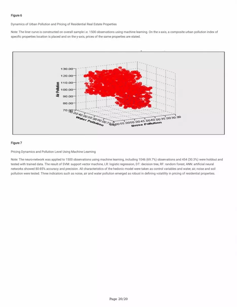
Figure 6
Dynamics of Urban Pollution and Pricing of Residential Real Estate Properties
Note: The liner curve is constructed on overall sample i.e. 1500 observations using machine learning. On the x-axis, a composite urban pollution index ofspeci�c properties location is placed and on the y-axis, prices of the same properties are stated.
Figure 7
Pricing Dynamics and Pollution Level Using Machine Learning
Note: The neuro-network was applied to 1500 observations using machine learning, including 1046 (69.7%) observations and 454 (30.3%) were holdout andtested with trained data. The result of SVM: support vector machine, LR: logistic regression, DT: decision tree, RF: random forest, ANN: arti�cial neuralnetworks showed 80-85% accuracy and precision. All characteristics of the hedonic model were taken as control variables and water, air, noise and soilpollution were tested. Three indicators such as noise, air and water pollution emerged as robust in de�ning volatility in pricing of residential properties.