SCHOOL OF ELECTRICAL AND ELECTRONICS

DEPARTMENT OF ELECTRONICS AND COMMMUNICATION ENGINEERING

UNIT – I

COMPUTER ARCHITECTURE AND OPERATING SYSTEM – SCS1315

UNIT.1 INTRODUCTION

Central Processing Unit - Introduction - General Register Organization - Stack organization --

Basic computer Organization - Computer Registers - Computer Instructions - Instruction Cycle.

Arithmetic, Logic, Shift Microoperations- Arithmetic Logic Shift Unit -Example Architectures:

MIPS, Power PC, RISC, CISC

Central Processing Unit

The part of the computer that performs the bulk of data-processing operations is called the central

processing unit CPU. The CPU is made up of three major parts, as shown in Fig.1

Fig 1. Major components of CPU.

The register set stores intermediate data used during the execution of the instructions.

The arithmetic logic unit (ALU) performs the required microoperations for executing the

instructions.

The control unit supervises the transfer of information among the registers and instructs

the ALU as to which operation to perform.

General Register Organization

When a large number of registers are included in the CPU, it is most efficient to connect

them through a common bus system. The registers communicate with each other not only for direct

data transfers, but also while performing various microoperations.

Hence it is necessary to provide a common unit that can perform all the arithmetic, logic,

and shift microoperations in the processor. A bus organization for seven CPU registers is shown

in Fig.2.

The output of each register is connected to two multiplexers (MUX) to form the two buses A

and B.

The selection lines in each multiplexer select one register or the input data for the particular

bus. The A and B buses form the inputs to a common arithmetic logic unit (ALU).

Fig 2 Register set with common ALU.

The operation selected in the ALU determines the arithmetic or logic microoperation that is to

be performed. The result of the microoperation is available for output data and also goes into

the inputs of all the registers. The register that receives the information from the output bus is

selected by a decoder. The decoder activates one of the register load inputs, thus providing a

transfer path between the data in the output bus and the inputs of the selected destination

register.

The control unit that operates the CPU bus system directs the information flow through the

registers and ALU by selecting the various components in the system.

For example, to perform the operation

R 1 <--R2 + R3

1. MUX A selector (SELA): to place the content of R2 into bus A.

2. MUX B selector (SELB): to place the content o f R 3 into bus B.

3. ALU operation selector (OPR): to provide the arithmetic addition A + B.

4. Decoder destination selector (SELD): to transfer the content of the output bus into R 1.

The four control selection variables are generated i n the control unit and must be available at the

beginning of a clock cycle.

Control Word

There are 14 binary selection inputs in the unit, and their combined value specifies a control

word. The 14-bit control word is defined in Fig. 4.

Fig 4. Control Word Format

TABLE 1 Encoding of Register Selection Fields

The encoding of the register selections is specified in Table 1. The 3-bit binary code listed

in the first column of the table specifies the binary code for each of the three fields. The register

selected by fields SELA, SELB, and SELD is the one whose decimal number is equivalent to the

binary number in the code. When SELA or SELB is 000, the corresponding multiplexer selects

the external input data. When SELD = 000, no destination register is selected but the contents of

the output.

The ALU provides arithmetic and logic operations. The shifter may be placed in the input

of the ALU to provide a preshift capability, or at the output of the ALU to provide postshifting

capability. In some cases, the shift operations are included with the ALU. The function table for

this ALU is listed in Fig.5. The encoding of the ALU operations for the CPU is specified in Table.

The OPR field has five bits and each operation is designated with a symbolic name.

Fig.5 Encoding of ALU Operations

Stack Organization:

A stack is a storage device that stores information in such a manner that the item stored

last is the first item retrieved. The operation of a stack can be compared to a stack of trays. The

last tray placed on top of the stack is the first to be taken off. The register that holds the address

for the stack is called a stack pointer (SP) because its value always points at the top item in the

stack. The two operations of a stack are the insertion and deletion of items. The operation of

insertion is called push. The operation of deletion is called pop.

Register Stack

A stack can be placed in a portion of a large memory or it can be organized as a collection

of a finite number of memory words or registers. Figure 6 shows the organization of a 64-word

register stack. The stack pointer register SP contains a binary number whose value is equal to the

address of the word that is currently on top of the stack. Three items are placed in the stack: A, B,

and C, in that order. Item C is on top of the stack so that the content of SP is now 3. To remove

the top item, the stack is popped by reading the memory word at address 3 and decrementing the

content of SP. Item B is now on top of the stack since SP holds address 2. To insert a new item,

the stack is pushed by incrementing SP and writing a word in the next-higher location in the stack.

Note that item C has been read out but not physically removed. This does not matter because when

the stack is pushed, a new item is written in its place.

The one-bit register FULL is set to 1 when the stack is full, and the one-bit register EMTY

is set to 1 when the stack is empty of items. DR is the data register that holds the binary data to be

written into or read out of the stack.

Initially, SP is cleared to 0, EMTY is set to 1, and FULL is cleared to 0, so that SP points

to the word at address 0 and the stack is marked empty and not full. If the stack is not full (if FULL

= 0), a new item is inserted with a push operation. The push operation is implemented with the

following sequence of microoperations:

DR <--M [SP] Read item from the top of stack

SP <--SP – 1 Decrement stack pointer

If (SP = 0) then (EMTY <--1) Check if stack is empty

FULL <--0 Mark the stack not full

Fig.6 Block diagram of a 64 word stack.

The top item is read from the stack into DR. The stack pointer is then decremented. If its

value reaches zero, the stack is empty, so EMTY is set to 1. This condition is reached if the item

read was in location L Once this item is read out, SP is decremented and reaches the value 0, which

is the initial value of SP.

Memory Stack:

A stack can exist as a stand-alone unit as in Fig. 6 or can be implemented in a random-

access memory attached to a CPU. The implementation of a stack in the CPU is done by assigning

a portion of memory to a stack operation and using a processor register as a stack pointer. Fig 7

shows a portion of computer memory partitioned into three segments: program, data, and stack.

The program counter PC points at the address of the next instruction in the program. The address

register AR points at an array of data. The stack pointer SP points at the top of the stack. The three

registers are connected to a common address bus, and either one can provide an address for

memory. PC is used during the fetch phase to read an instruction. AR is used during the execute

phase to read an operand. SP is used to push or pop items into or from the stack. As shown in

Fig.7, the initial value of SP is 4001 and the stack grows with decreasing addresses. Thus the first

item stored in the stack is at address 4000, the second item is stored at address 3999, and the last

address that can be used for the stack is 3000. No provisions are available for stack limit checks.

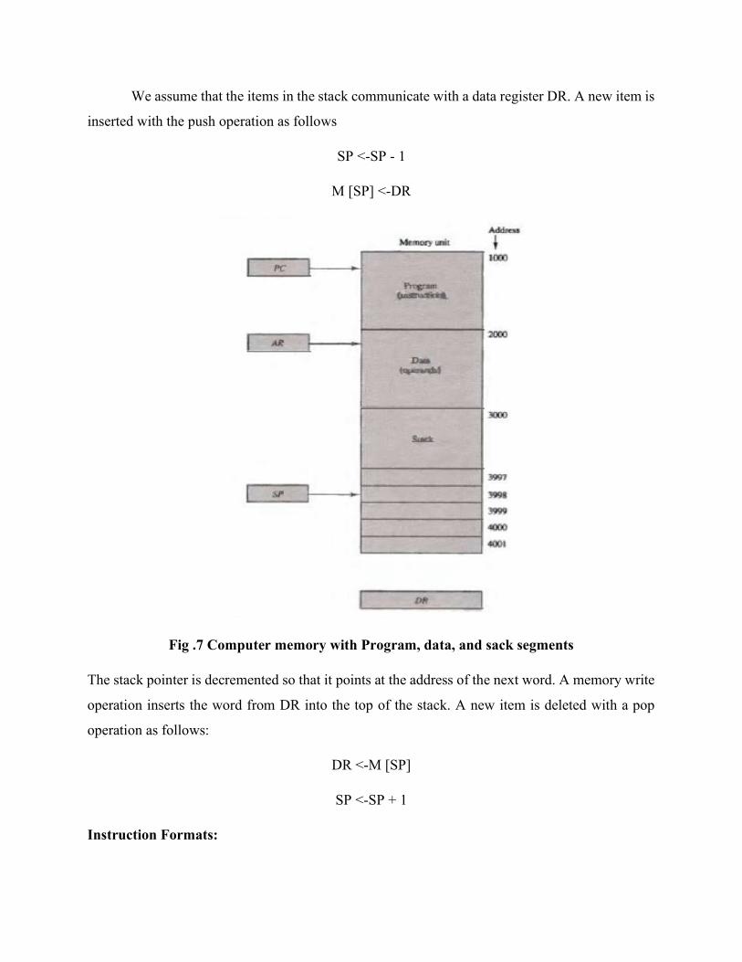
We assume that the items in the stack communicate with a data register DR. A new item is

inserted with the push operation as follows

SP <-SP - 1

M [SP] <-DR

Fig .7 Computer memory with Program, data, and sack segments

The stack pointer is decremented so that it points at the address of the next word. A memory write

operation inserts the word from DR into the top of the stack. A new item is deleted with a pop

operation as follows:

DR <-M [SP]

SP <-SP + 1

Instruction Formats:

The format of an instruction is usually depicted in a rectangular box symbolizing the bits

of the instruction as they appear in memory words or in a control register. The bits of the instruction

are divided into groups called fields. The most common fields found in instruction formats are:

1. An operation code field that specifies the operation to be performed.

2. An address field that designates a memory address or a processor register.

3. A mode field that specifies the way the operand or the effective address is determined.

The operation code field of an instruction is a group of bits that define various processor

operations, such as add, subtract, complement, and shift.

Three-Address Instructions

Computers with three-address instruction formats can use each address field to specify

either a processor register or a memory operand. The program in assembly language that

evaluates X = (A + B) • (C + D) is shown below, together with comments that explain the

register transfer operation of each instruction.

ADD R 1, A, B R 1 <--M [A] + M [B]

ADD R2, C, D R2 <--M [C] + M [D]

MUL X, R 1, R 2 M [X] <--R 1 • R 2

It is assumed that the computer has two processor registers, R 1 and R2. The symbol M [A]

denotes the operand at memory address symbolized by A. The advantage of the three-address

format is that it results in short programs when evaluating arithmetic expressions. The

disadvantage is that the binary-coded instructions require too many bits to specify three

addresses.

Two-Address Instructions

Two-address instructions are the most common in commercial computers. Here again each

address field can specify either a processor register or a memory word. The program to evaluate

X = (A + B) • (C + D) is as follows:

MOV R 1, A R 1 <--M [A]

ADD R 1, B R 1 <--R 1 + M [B]

MOV R 2, C R2 <--M [C]

ADD R2, D R2 <--R 2 + M [D]

MUL R1, R2 R 1 <--R 1 • R 2

MOV X, R 1 M [X] <--R 1

The MOV instruction moves or transfers the operands t o and from memory and processor

registers. The first symbol listed in an instruction is assumed to be both a source and the destination

where the result of the operation is transferred.

One-Address Instructions

One-address instructions use an implied accumulator (AC) register for all data

manipulation. For multiplication and division there is a need for a second register. The program to

evaluate

X = (A + B) • (C + D) is

L O A D A AC <- M [A]

A DD B A C <- A C + M [B]

S T O R E T M [T] <- A C

L O A D C A C <- M [C]

A D D D A C <- A C + M [D]

M U L T A C <- A C • M [T]

S T O R E X M [X] <- A C

Zero-Address Instructions

A stack-organized computer does not use an address field for the instructions ADD and

MUL. The PUSH and POP instructions, however, need an address field to specify the operand that

communicates with the stack. The following program shows how X = (A + B) • (C + D) will be

written for a stack organized computer. (TOS stands for top of stack.)

P U S H A T O S <- A

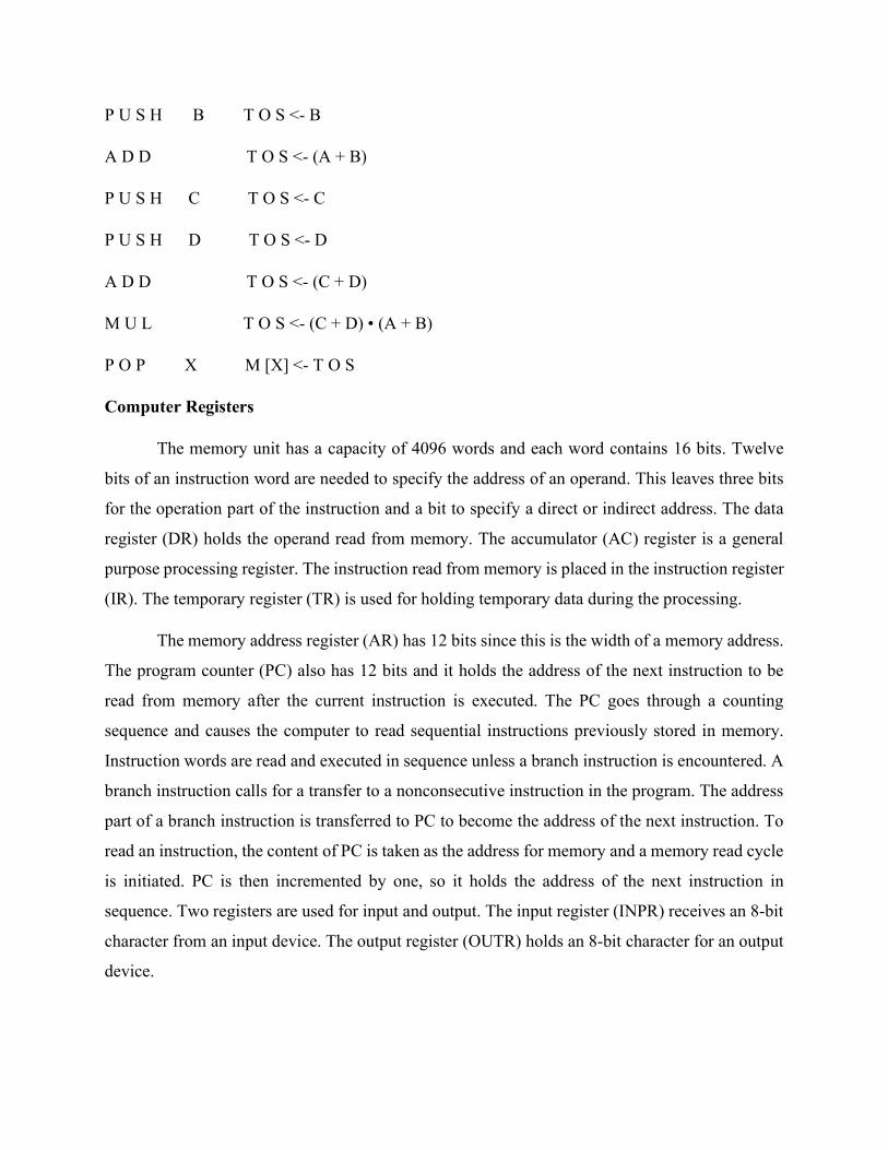
P U S H B T O S <- B

A D D T O S <- (A + B)

P U S H C T O S <- C

P U S H D T O S <- D

A D D T O S <- (C + D)

M U L T O S <- (C + D) • (A + B)

P O P X M [X] <- T O S

Computer Registers

The memory unit has a capacity of 4096 words and each word contains 16 bits. Twelve

bits of an instruction word are needed to specify the address of an operand. This leaves three bits

for the operation part of the instruction and a bit to specify a direct or indirect address. The data

register (DR) holds the operand read from memory. The accumulator (AC) register is a general

purpose processing register. The instruction read from memory is placed in the instruction register

(IR). The temporary register (TR) is used for holding temporary data during the processing.

The memory address register (AR) has 12 bits since this is the width of a memory address.

The program counter (PC) also has 12 bits and it holds the address of the next instruction to be

read from memory after the current instruction is executed. The PC goes through a counting

sequence and causes the computer to read sequential instructions previously stored in memory.

Instruction words are read and executed in sequence unless a branch instruction is encountered. A

branch instruction calls for a transfer to a nonconsecutive instruction in the program. The address

part of a branch instruction is transferred to PC to become the address of the next instruction. To

read an instruction, the content of PC is taken as the address for memory and a memory read cycle

is initiated. PC is then incremented by one, so it holds the address of the next instruction in

sequence. Two registers are used for input and output. The input register (INPR) receives an 8-bit

character from an input device. The output register (OUTR) holds an 8-bit character for an output

device.

Fig .8 List of Registers for the Basic Computer

Figure 9. Basic computer registers and memory.

Computer Instructions:

The basic computer has three instruction code formats, as shown in Fig. 10. Each format

has 16 bits. The operation code (opcode) part of the instruction contains three bits and the

meaning of the remaining 13 bits depends on the operation code encountered.

A memory-reference instruction uses 12 bits to specify an address and one bit to specify

the addressing mode I. I is equal to 0 for direct address and to 1 for indirect address. The

register reference instructions are recognized by the operation code 111 with a 0 in the

leftmost bit (bit 15) of the instruction.

A register-reference instruction specifies an operation on or a test of the AC register. An

operand from memory is not needed; therefore, the other 12 bits are used to specify the

operation or test to be executed.

A input-output instruction does not need a reference to memory and is recognized by the

operation code Ill with a 1 in the leftmost bit of the instruction. The remaining 12 bits are

used to specify the type of input-output operation or test performed.

The type of instruction is recognized by the computer control from the four bits in positions

12 through 15 of the instruction. If the three opcode bits in positions 12 through 14 are not equal

to 111, the instruction is a memory-reference type and the bit in position 15 is taken as the

addressing mode I. If the 3-bit opcode is equal to 111, control then inspects the bit in position 15.

If this bit is 0, the instruction is a register-reference type. If the bit is 1, the instruction is an input

-output type. Note that the bit in position 15 of the instruction code is designated by the symbol I

but is not used as a mode bit when the operation code is equal to 111.

Fig 10. Basic computer instruction formats.

Fig 11.Basic Computer Instructions

Stack Organization:

Stack is a storage device that stores information in a way that the item is stored last is the first to

be retrieved (LIFO). Stack in computers is actually a memory unit with address register (stack

pointer SP) that can count only. SP value always points at top item in stack.

The two operations done on stack are,

PUSH (Push Down), operation of insertion of items into stack

POP (Pop Up), operation of deletion item from stack

Those operation are simulated by INC and DEC stack register (SP).

1. Register stack:

A stand alone unit that consists of collection of finite number of registers. The next

example shows 64 location stack unit with SP that stores address of the word that is

currently on the top of stack.

Note that 3 items are placed in the stack A, B, and C. Item C is in top of stack so that SP

holds 3 which the address of item C. To remove top item from stack (popping stack) we

start by reading content of address 3 and decrementing the content of SP. Item B is now in

top of stack holding address 2.

To insert new item (pushing the stack) we start by incrementing SP then writing a new

word where SP now points to (top of stack).

Note that in 64-word stack we need to have SP of 6 bits only (from 000000 to 111111). If

111111 is reached then at next push SP will be 000000, that is when the stack is FULL.

Similarly, when SP is 000001 then at next pop SP will go to 000000 that is when the stack

is EMTY.

Initially, SP = 0, EMPTY = 1, FULL =0

Procedures for pushing stack

SP <- SP + 1

M[SP] <- DR

IF (SP = 0) THEN (FULL = 1)

EMTY <- 0

Note that:

1. Always we use DR to pass word into stack

2. M[SP] memory word specified by address currently in SP

3. First item stored in stack is at address 1

4. Last item stored in stack is at address 0. That is FULL = 1

5. Any push to stack means EMTY = 0

2. Memory Stack :

Stack can be implemented in RAM memory attached to CPU. Only by assigning

special part of it for stack operations.

Next figure shows of main memory divided into program, data, and stack.

PC points to next instruction in instruction part

AR points to array of data of operands

SP points to top of stack All are connected to common address bus

Stack grows (pushed) with decreasing address and empties (pops) with increasing

address.

New item is inserted with push operation by decrementing SP then a write to SP

address is done

SP <-SP -1

M [SP]<- DR

Last item is removed from stack with pop operation by removing item by reading

from memory location addressed by SP then SP is incremented.

DR <- M [SP]

SP <- SP +1

As shown in figure initial value of SP is 4001 and first item when pushed in stack stores at

address 4000 and second one stores at address 3999. The last address pushed into will be

3000. (See limitation danger?)

Most computers are not supported by hardware to sense stack overflow and underflow. But

can be implemented by saving the 2 limits in 2 registers. After each push or pop the SP is

compared with the limit to see if stack has reached its limits. So must be taking care of

using software.

Always in this way we load SP with bottom address of stack portion of memory

Reverse Polish Notation:

Very useful notation to utilize stacks to evaluate arithmetic expressions.

We write in infix notation such as:

A*B + C*D

We compute A*B, store product, compute C*D, then sum two products. So we have to scam back

and forth to see which operation comes first.

The 3 notations to evaluate expressions

1. A + B Infix notation

2. +AB Prefix notation (Polish notation)

3. AB+ Postfix notation (reverse Polish

Reverse Polish Notation is in a form suitable for stack manipulation. Starts by scanning expression

from left to right. When operator is found then perform

Instruction Format:

Operation with 2 operands in left of operator and replace result place of 2 operands and operator.

Then you can continue this until you reach final answer.

Example

Expression A*B + C*D is written in RPN as AB*CD*+. And will computed as

(A*B) CD *+

(A*B)(C*D) +

Example

Convert infix notation expression (A + B)*(C * (D + E) + F) to RPN?

AB+ DE+ C * F+*.

Will be computed as

(A+B) (D+E) C * F + *

Reverse polish notation combined with stack comprised of registers is most efficient way

to evaluate expression. Stacks are good for handling long and complex problems involving

chain calculations. But need first to convert arithmetic expressions into parenthesis-free

reverse polish notation.

This procedure is employed in some scientific calculators and some computers.

Example

Convert (3*4) (5*6) to RPN

34*56*+

The Instruction coding fields in today’s computers follow the next format

1. Operation code field to specify operation

2. Address field that specifies operand address field or register

3. Mode field to specify effective address

In general, most processors are organized in one of 3 ways

Single register (Accumulator) organization

Basic Computer is a good example

Accumulator is the only general-purpose register

General register organization

Used by most modern computer processors

Any of the registers can be used as the source or destination for computer operations

Stack organization

All operations are done using the hardware stack

For example, an OR instruction will pop the two top elements from the stack, do a

logical OR on them, and push the result on the stack

We are interested with address field of instructions with multiple address fields in

instructions. The number of address fields in the instruction format depends on the internal

organization of CPU. Some CPU combines features from more of one structure.

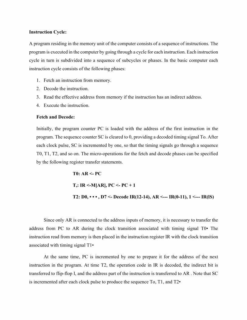
Instruction Cycle:

A program residing in the memory unit of the computer consists of a sequence of instructions. The

program is executed in the computer by going through a cycle for each instruction. Each instruction

cycle in turn is subdivided into a sequence of subcycles or phases. In the basic computer each

instruction cycle consists of the following phases:

1. Fetch an instruction from memory.

2. Decode the instruction.

3. Read the effective address from memory if the instruction has an indirect address.

4. Execute the instruction.

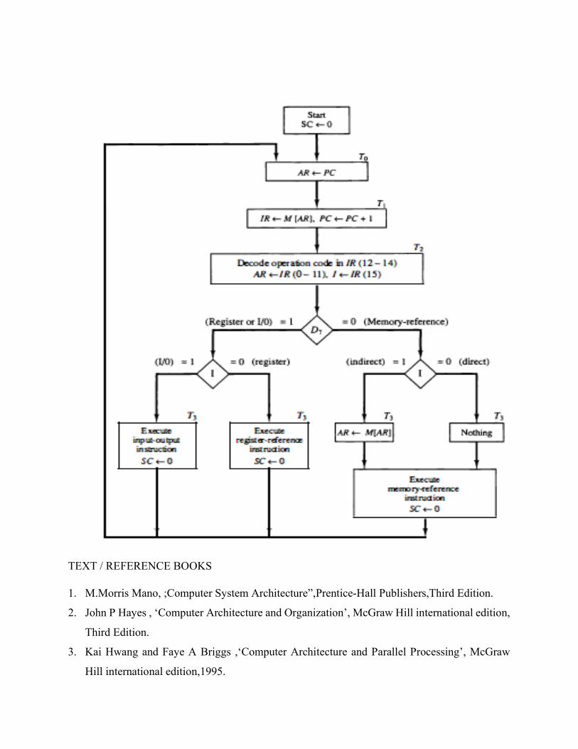
Fetch and Decode:

Initially, the program counter PC is loaded with the address of the first instruction in the

program. The sequence counter SC is cleared to 0, providing a decoded timing signal To. After

each clock pulse, SC is incremented by one, so that the timing signals go through a sequence

T0, T1, T2, and so on. The micro-operations for the fetch and decode phases can be specified

by the following register transfer statements.

T0: AR <- PC

T,: IR <-M[AR], PC <- PC + 1

T2: D0, • • • , D7 <- Decode IR(12-14), AR <--- IR(0-11), 1 <--- IR(lS)

Since only AR is connected to the address inputs of memory, it is necessary to transfer the

address from PC to AR during the clock transition associated with timing signal T0• The

instruction read from memory is then placed in the instruction register IR with the clock transition

associated with timing signal T1•

At the same time, PC is incremented by one to prepare it for the address of the next

instruction in the program. At time T2, the operation code in IR is decoded, the indirect bit is

transferred to flip-flop I, and the address part of the instruction is transferred to AR . Note that SC

is incremented after each clock pulse to produce the sequence To, T1, and T2•

TEXT / REFERENCE BOOKS

1. M.Morris Mano, ;Computer System Architecture”,Prentice-Hall Publishers,Third Edition.

2. John P Hayes , ‘Computer Architecture and Organization’, McGraw Hill international edition,

Third Edition.

3. Kai Hwang and Faye A Briggs ,‘Computer Architecture and Parallel Processing’, McGraw

Hill international edition,1995.

SCHOOL OF ELECTRICAL AND ELECTRONICS

DEPARTMENT OF ELECTRONICS AND COMMMUNICATION ENGINEERING

UNIT – II

COMPUTER ARCHITECTURE AND OPERATING SYSTEM– SCS1315

UNIT 2 CONTROL UNIT DESIGN AND MULTIPROCESSORS

Microprogrammed Control: Control memory - address sequencing - Microprogram Example-

Design of Control unit -Example Processor design Multiprocessors: Characteristics-

Interprocessor Arbitration- Interprocessor Communication

Control Memory:

The function of the control unit in a digital computer is to initiate sequences of microoperations.

The number of different types of microoperations that are available in a given system is finite.

Microprogramming is a second alternative for designing the control unit of a digital computer. The

control function that specifies a microoperation is a binary variable. When it is in one binary state,

the corresponding rnicrooperation is executed.

In a bus-organized system, the control signals that specify microoperations are groups of

bits that select the paths in multiplexers, decoders, and arithmetic logic units. The control unit

initiates a series of sequential steps of rnicrooperations. The control variables at any given time

can be represented by a string of 1's and 0's called a control word. As such, control words can be

programmed to perform various operations on the components of the system.

A control unit whose binary control variable are stored in memory is called a

microprogrammed control unit. Each word in control memory contains within it a

microinstruction. The microinstruction specifies one or more microoperations for the system. A

sequence of microinstructions constitutes a microprogram. Since alterations of the microprogram

are not needed once the control unit is in operation, the control memory can be a read-only memory

(ROM).

A more advanced development known as dynamic microprogramming permits a

microprogram to be loaded initially from an auxiliary memory such as a magnetic disk. Control

units that use dynamic microprogramming employ a writable control memory. This type of

memory can be used for writing (to change the microprogram) but is used mostly for reading. A

memory that is part of a control unit is referred to as a control memory.

A computer that employs a microprogrammed control unit will have two separate

memories:

a main memory and

a control memory.

The main memory is available to the user for storing the programs. The contents of

main memory may alter when the data are manipulated and every time that the program

is changed. The user's program in main memory consists of machine instructions and

data. In contrast, the control memory holds a fixed microprogram that cannot be altered

by the occasional user. The microprogram consists of microinstructions that specify

various internal control signals for execution of register microoperations.

Each machine instruction initiates a series of microinstructions in control memory.

These microinstructions generate the microoperations to fetch the instruction from

main memory; to evaluate the effective address, to execute the operation specified by

the instruction, and to return control to the fetch phase in order to repeat the cycle for

the next instruction

Fig 1. Microprogrammed control organization

The general configuration of a microprogrammed control unit is demonstrated in

the block diagram of Fig 1.

The control memory is assumed to be a ROM, within which all control

information is permanently stored.

The control memory address register specifies the address of the

microinstruction, and the control data register holds the microinstruction

read from memory.

The microinstruction contains a control word that specifies one or more

microoperations for the data processor.

Once these operations are executed, the control must determine the next

address. The location of the next microinstruction may be the one next in

sequence, or it may be located somewhere else in the control memory.

While the microoperations are being executed, the next address is computed

in the next address generator circuit and then transferred into the control

address register to read the next microinstruction.

The next address generator is sometimes called a microprogram sequencer,

as it determines the address sequence that is read from control memory.

Typical functions of a microprogram sequencer are incrementing the

control address register by one, loading into the control address register an

address from control memory, transferring an external address, or loading

an initial address to start the control operations.

The control data register holds the present microinstruction while the next

address is computed and read from memory. The data register is sometimes

called a pipeline register. It allows the execution of the microoperations

specified by the control word simultaneously with the generation of the next

microinstruction.

Address Sequencing:

Microinstructions are stored in control memory in groups, with each group specifying a

routine. Each computer instruction has its own microprogram routine in control memory to

generate the microoperations that execute the instruction. The hardware that controls the address

sequencing of the control memory must be capable of sequencing the microinstructions within a

routine and be able to branch from one routine to another. The steps that the control must undergo

during the execution of a single computer instruction.

An initial address is loaded into the control address register (CAR) when power is

turned on in the computer. This address is usually the address of the first

microinstruction that activates the instruction fetch routine.

The fetch routine may be sequenced by incrementing the control address register

through the rest of its microinstructions. At the end of the fetch routine, the

instruction I in the instruction register of the computer.

The control memory next must go through the routine that determines the effective

address of the operand.

The effective address computation routine in control memory can be reached

through a branch microinstruction, which is conditioned on the status of the mode

bits of the instruction. When the effective address computation routine is

completed, the address of the operand is available in the memory address register.

The next step is to generate the microoperations that execute the instruction fetched

from memory. The microoperation steps to be generated in processor registers

depend on the operation code part of the instruction.

Each instruction has its own microprogram routine stored in a given location of

control memory. The transformation from the instruction code bits to an address in

control memory where the routine is located is referred to as a mapping process.

A mapping procedure is a rule that transforms the instruction code into a control

memory address. Once the required routine is reached, the microinstructions that

execute the instruction may be sequenced by incrementing the control address

register, but sometimes the sequence of microoperations will depend on values of

certain status bits in processor registers.

When the execution of the instruction is completed, control must return to

the fetch routine. This is accomplished by executing an unconditional branch

microinstruction to the first address of the fetch routine. In summary, the address

sequencing capabilities required in a control memory are:

1. Incrementing of the control address register.

2. Unconditional branch or conditional branch, depending on status bit conditions.

3. A mapping process from the bits of the instruction to an address for control

memory.

4. A facility for subroutine call and return.

Microprogram Example: The process of code generation for the control memory is called microprogramming. The block diagram of the computer configuration is shown in below figure. Two memory units:

Main memory – stores instructions and data Control memory – stores microprogram

Four processor registers Program counter – PC Address register – AR Data register – DR Accumulator register - AC

Two control unit registers Control address register – CAR Subroutine register – SBR

Transfer of information among registers in the processor is through MUXs rather than a

bus.

The computer instruction format is shown in below figure.

Three fields for an instruction: 1-bit field for indirect addressing 4-bit opcode 11-bit address field

Design of control Unit: The control memory out of each subfield must be decoded to provide the distinct

microoperations. The outputs of the decoders are connected to the appropriate inputs in the processor unit. The below figure shows the three decoders and some of the connections that must be

made from their outputs.

The three fields of the microinstruction in the output of control memory are decoded with

a 3x8 decoder to provide eight outputs. Each of the output must be connected to proper circuit to initiate the corresponding micro

operation. When F1 = 101 (binary 5), the next pulse transition transfers the content of DR (0-10) to

AR. Similarly, when F1= 110 (binary 6) there is a transfer from PC to AR (symbolized by

PCTAR). As shown in Fig, outputs 5 and 6 of decoder F1 are connected to the load input of AR so that when either one of these outputs is active, information from the multiplexers is transferred to AR.

The multiplexers select the information from DR when output 5 is active and from PC when output 5 is inactive.

The transfer into AR occurs with a clock transition only when output 5 or output 6 of the decoder is active.

For the arithmetic logic shift unit the control signals are instead of coming from the logical gates, now these inputs will now come from the outputs of AND, ADD and DRTAC respectively.

lnterprocessor Arbitration

Computer systems contain a number of buses at various levels to facilitate the transfer of information between components. The CPU contains a number of internal buses for transferring information between processor registers and ALU.

A memory bus consists of lines for transferring data, address, and read/write information.

An I/O bus is used to transfer information to and from input and output devices.

A bus that connects major components in a multiprocessor system, such as CPUs, lOPs,

and memory, is called a system bus.

In a synchronous bus, each data item is transferred during a time slice known in advance to both source and destination units. Synchronization is achieved by driving both units from a common clock source.

In an asynchronous bus, each data item being transferred is accompanied by handshaking control signals to indicate when the data are transferred from the source and received by the destination.

Serial Arbitration Procedure Arbitration procedures service all processor requests on the basis of established priorities. A hardware bus priority resolving technique can be established by means of a serial or parallel connection of the units requesting control of the system bus. The serial priority resolving technique is obtained from a daisy-chain connection of bus arbitration circuits similar to the priority interrupt logic. The processors connected to the system bus are assigned priority according to their position along the priority control line. The device closest to the priority line is assigned the highest priority. When multiple devices concurrently request the use of the bus, the device with the highest priority is granted access to it.

The below Figure shows the daisy-chain connection of four arbiters. It is assumed that each processor has its own bus arbiter logic with priority-in and priority-out lines.

The priority out (PO) of each arbiter is connected to the priority in (PI) of the next-lower-priority arbiter. The PI of the highest-priority unit is maintained at a logic 1 value. The highest-priority unit in the system will always receive access to the system bus when it requests it. The PO output for a particular arbiter is equal to 1 if its PI input is equal to 1 and the processor associated with the arbiter logic is not requesting control of the bus. This is the way that priority is passed to the next unit in the chain. If the processor requests control of the bus and the corresponding arbiter finds its PI input equal to 1, it sets its PO output to 0. Lower-priority arbiters receive a 0 in PI and generate a 0 in PO. Thus the processor whose arbiter has a PI = 1 and PO = 0 is the one that is given control of the system bus. A processor may be in the middle of a bus operation when a higher- priority processor requests the bus. The lower-priority processor must complete its bus operation before it relinquishes control of the bus. The bus busy line shown in Figure. It provides a mechanism for an orderly transfer of control. The busy line comes from open-collector circuits in each unit and provides a wired-OR logic connection. When an arbiter receives control of the bus (because it’s PI = 1 and PO = 0) it examines the busy line. If the line is inactive, it means that no other processor is using the bus. The arbiter activates the busy line and its processor takes control of the bus. However, if the arbiter finds the busy line active, it means that another processor is currently using the bus. The arbiter keeps examining the busy line while the lower-priority processor that lost control of the bus completes its operation. When the bus busy line returns to its inactive state, the higher-priority arbiter enables the busy line, and its corresponding processor can then conduct the required bus transfers. Parallel Arbitration Logic The parallel bus arbitration technique uses an external priority encoder and a decoder as shown in Figure. Each bus arbiter in the parallel scheme has a bus request output line and

a bus acknowledge input line. Each arbiter enables the request line when its processor is requesting access to the system bus.

The processor takes control of the bus if its acknowledge input line is enabled. The bus busy line provides an orderly transfer of control, as in the daisy-chaining case. Figure shows the request lines from four arbiters going into a 4 x 2 priority encoder. The output of the encoder generates a 2-bit code which represents the highest-priority unit among those requesting the bus. The 2-bit code from the encoder output drives a 2 x 4 decoder which enables the proper acknowledge line to grant bus access to the highest-priority unit. The bus priority-in BPRN and bus priority-out BPRO are used for a daisy-chain connection of bus arbitration circuits. The bus busy signal BUSY is an open-collector output used to instruct all arbiters when the bus is busy conducting a transfer. The common bus request CBRQ is also an open-collector output that serves to instruct the arbiter if there are any other arbiters of lower-priority requesting use of the system bus. The signals used to construct a parallel arbitration procedure are bus request BREQ and priority-in BPRN, corresponding to the request and acknowledge signals .The bus clock BCLK is used to synchronize all bus transactions.

lnterprocessor Communication The instruction set of a multiprocessor contains basic instructions that are used to implement communication and synchronization between cooperating processes. Communication refers to the exchange of data between different processes. For example, parameters passed to a procedure in a different processor constitute interprocessor communication. Synchronization refers to the special case where the data used to communicate between processors is control information. Synchronization is needed to enforce the correct sequence of processes and to ensure mutually exclusive access to shared writable data. Mutual Exclusion with a Semaphore A properly functioning multiprocessor system must provide a mechanism that will guarantee orderly access to shared memory and other shared resources. This is necessary to protect data from being changed simultaneously by two or more processors. This mechanism has been termed mutual exclusion. Mutual exclusion must be provided in a multiprocessor system to enable one processor to exclude or lock out access to a shared resource by other processors when it is in a critical section. A critical section is a program sequence that, once begun, must complete execution before another processor accesses the same shared resource. A binary variable called a semaphore is often used to indicate whether or not a processor is executing a critical section. A semaphore is a software- controlled flag that is stored in a memory location that all processors can access. When the semaphore is equal to 1, it means that a processor is executing a critical program, so that the shared memory is not available to other processors. When the semaphore is equal to 0, the shared memory is available to any requesting processor. Processors that share the same memory segment agree by convention not to use the memory segment unless the semaphore is equal to 0, indicating that memory is available. They also agree to set the semaphore to 1 when they are executing a critical section and to clear it to 0 when they are finished. Testing and setting the semaphore is itself a critical operation and must be performed as a single indivisible operation. If it is not, two or more processors may test the semaphore simultaneously and then each set it, allowing them to enter a critical section at the same time. This action would allow simultaneous execution of critical section, which can result in erroneous initialization of control parameters and a loss of essential information. A semaphore can be initialized by means of a test and set instruction in conjunction with a hardware lock mechanism. A hardware lock is a processor- generated signal that serves to prevent other processors from using the system bus as long as the signal is active. The test-and-set instruction tests and sets a semaphore and activates the lock mechanism during the time that the instruction is being executed. This prevents other processors from changing the semaphore between the time that the processor is testing it and the time that it is setting it. Assume that the

semaphore is a bit in the least significant position of a memory word whose address is symbolized by SEM. Let the mnemonic TSL designate the "test and set while locked" operation. The instruction TSL SEM will be executed in two memory cycles (the first to read and the second to write) without interference as follows: R + -M [SEM] Test semaphore M [SEM] + ->1 Set semaphore The semaphore is tested by transferring its value to a processor register R and then it is set to 1. The value in R determines what to do next. If the processor finds that R = 1, it knows that the semaphore was originally set. (The fact that it is set again does not change the semaphore value.) That means that another processor is executing a critical section, so the processor that checked the semaphore does not access the shared memory. If R = 0, it means that the common memory (or the shared resource that the semaphore represents) is available. The semaphore is set to 1 to prevent other processors from accessing memory. The processor can now execute the critical section. The last instruction in the program must clear location SEM to zero to release the shared resource to other processors. Note that the lock signal must be active during the execution of the test-and-set instruction. It does not have to be active once the semaphore is set. Thus the lock mechanism prevents other processors from accessing memory while the semaphore is being set. The semaphore itself, when set, prevents other processors from accessing shared memory while one processor is executing a critical section. TEXT / REFERENCE BOOKS

1. M.Morris Mano, ;Computer System Architecture”,Prentice-Hall Publishers,Third Edition.

2. John P Hayes , ‘Computer Architecture and Organization’, McGraw Hill international edition,

Third Edition.

3. Kai Hwang and Faye A Briggs ,‘Computer Architecture and Parallel Processing’, McGraw

Hill international edition,1995.

SCHOOL OF ELECTRICAL AND ELECTRONICS

DEPARTMENT OF ELECTRONICS AND COMMMUNICATION

ENGINEERING

UNIT – III

COMPUTER ARCHITECTURE AND OPERATING SYSTEM– SCS1315

UNIT.3 MEMORY AND I/O SYSTEM

Memory Organization: Memory Hierarchy - Main memory - auxiliary Memory - Associative

Memory –Cache Memory - Virtual memory Input - Output Organization: Peripheral Devices -

I/O Interface, Modes of transfer - Priority Interrupt - DMA - IOP - Serial Communication

Memory Hierarchy

The memory unit is an essential component in any digital computer since It Is needed for

storing programs and data. The memory unit that communicates directly with the CPU is called

the main memory. Devices that provide backup storage are called auxiliary memory. The most

common auxiliary memory devices used in computer systems are magnetic disks and tapes. They

are used for storing system programs, large data files, and other backup information. The

memory hierarchy system consists of all storage devices employed in a computer system from

the slow but high-capacity auxiliary memory to a relatively faster main memory, to an even

smaller and faster cache memory accessible to the high-speed processing logic. Figure 1

illustrates the components in a typical memory hierarchy.

Fig.1 Memory hierarchy in a typical Computer system

Cache Memory:

A special very- high- speed memory called a Cache is sometimes used to increase the

speed of processing by making current programs and data available to the CPU at a rapid rate.

The cache memory is employed in computer systems to compensate for the speed differential

between main memory access time and processor logic. CPU logic is usually faster than main

memory access time, with the result that processing speed is limited primarily by the speed of

main memory.

A technique used to compensate for the mismatch in operating speeds is to employ an

extremely fast, small cache between the CPU and main memory whose access time Is dose to

processor logic dock cycle time. The cache is used for storing segments of programs currently

being executed in the CPU and temporary data frequently needed in the present calculations.

Cache Memory

Analysis of a large number of typical programs has shown that the references to memory

at any given interval of time tend to be confined within a few localized areas in memory. This

phenomenon is known as the property of locality of reference locality of reference. When a

program loop is executed, the CPU repeatedly refers to the set of instructions in memory that

constitute the loop. Every time a given subroutine is called, its set of instructions are fetched

from memory. Thus loops and subroutines tend to localize the references to memory for fetching

instructions. The result of all these observations is the locality of reference property, which states

that over a short interval of time, the addresses generated by a typical program refer to a few

localized areas of memory repeatedly, while the remainder of memory is accessed relatively

infrequently.

If the active portions of the program and data are placed in a fast small memory, the

average memory access time can be reduced, thus reducing the total execution time of the

program. Such a fast small memory is referred to as a cache memory. It is placed between the

CPU and main memory as shown in the fig 2.

Fig 2. Example of cache memory.

Virtual Memory

Virtual Memory is a storage allocation scheme in which secondary memory can be addressed as

though it were part of main memory. The addresses a program may use to reference memory are

distinguished from the addresses the memory system uses to identify physical storage sites, and

program generated addresses are translated automatically to the corresponding machine

addresses.

The size of virtual storage is limited by the addressing scheme of the computer system and

amount of secondary memory is available not by the actual number of the main storage

locations.

It is a technique that is implemented using both hardware and software. It maps memory

addresses used by a program, called virtual addresses, into physical addresses in computer

memory.

1. All memory references within a process are logical addresses that are dynamically

translated into physical addresses at run time. This means that a process can be swapped

in and out of main memory such that it occupies different places in main memory at

different times during the course of execution.

2. A process may be broken into number of pieces and these pieces need not be

continuously located in the main memory during execution. The combination of dynamic

run-time address translation and use of page or segment table permits this.

Virtual memory is commonly implemented by demand paging. It can also be implemented in a

segmentation system. Demand segmentation can also be used to provide virtual memory.

Demand Paging

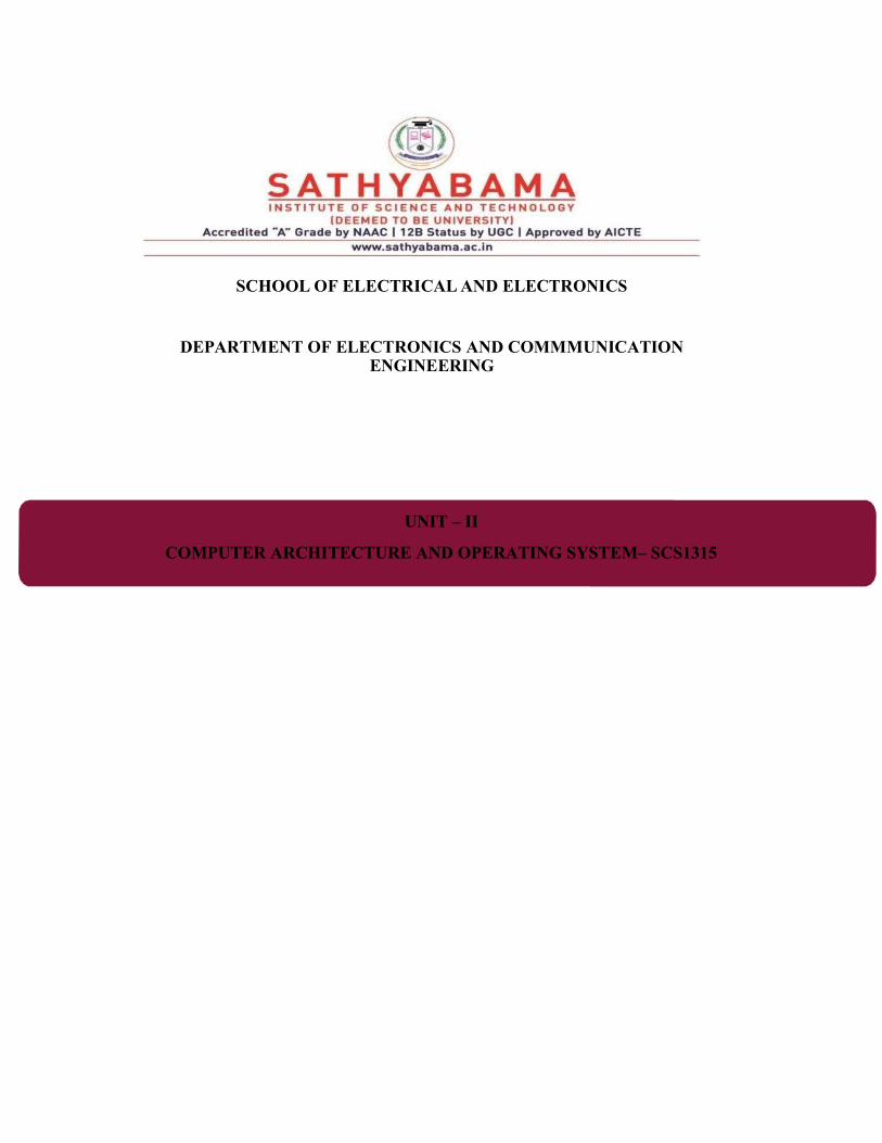
A demand paging system is quite similar to a paging system with swapping where processes

reside in secondary memory and pages are loaded only on demand, not in advance. When a

context switch occurs, the operating system does not copy any of the old program’s pages out

to the disk or any of the new program’s pages into the main memory Instead, it just begins

executing the new program after loading the first page and fetches that program’s pages as they

are referenced.

While executing a program, if the program references a page which is not available in the main

memory because it was swapped out a little ago, the processor treats this invalid memory

reference as a page fault and transfers control from the program to the operating system to

demand the page back into the memory.

Advantages

Following are the advantages of Demand Paging −

Large virtual memory.

More efficient use of memory.

There is no limit on degree of multiprogramming.

Disadvantages

Number of tables and the amount of processor overhead for handling page interrupts are

greater than in the case of the simple paged management techniques.

Page Replacement Algorithm

Page replacement algorithms are the techniques using which an Operating System decides

which memory pages to swap out, write to disk when a page of memory needs to be allocated.

Paging happens whenever a page fault occurs and a free page cannot be used for allocation

purpose accounting to reason that pages are not available or the number of free pages is lower

than required pages.

When the page that was selected for replacement and was paged out, is referenced again, it has

to read in from disk, and this requires for I/O completion. This process determines the quality

of the page replacement algorithm: the lesser the time waiting for page-ins, the better is the

algorithm.

A page replacement algorithm looks at the limited information about accessing the pages

provided by hardware, and tries to select which pages should be replaced to minimize the total

number of page misses, while balancing it with the costs of primary storage and processor time

of the algorithm itself. There are many different page replacement algorithms. We evaluate an

algorithm by running it on a particular string of memory reference and computing the number

of page faults,

Reference String

The string of memory references is called reference string. Reference strings are generated

artificially or by tracing a given system and recording the address of each memory reference.

The latter choice produces a large number of data, where we note two things.

For a given page size, we need to consider only the page number, not the entire address.

If we have a reference to a page p, then any immediately following references to

page p will never cause a page fault. Page p will be in memory after the first reference;

the immediately following references will not fault.

For example, consider the following sequence of addresses − 123,215,600,1234,76,96

If page size is 100, then the reference string is 1,2,6,12,0,0

First In First Out (FIFO) algorithm

Oldest page in main memory is the one which will be selected for replacement.

Easy to implement, keep a list, replace pages from the tail and add new pages at the

head.

Optimal Page algorithm

An optimal page-replacement algorithm has the lowest page-fault rate of all algorithms.

An optimal page-replacement algorithm exists, and has been called OPT or MIN.

Replace the page that will not be used for the longest period of time. Use the time when

a page is to be used.

Least Recently Used (LRU) algorithm

Page which has not been used for the longest time in main memory is the one which will

be selected for replacement.

Easy to implement, keep a list, replace pages by looking back into time.

Page Buffering algorithm

To get a process start quickly, keep a pool of free frames.

On page fault, select a page to be replaced.

Write the new page in the frame of free pool, mark the page table and restart the

process.

Now write the dirty page out of disk and place the frame holding replaced page in free

pool.

Least frequently Used (LFU) algorithm

The page with the smallest count is the one which will be selected for replacement.

This algorithm suffers from the situation in which a page is used heavily during the

initial phase of a process, but then is never used again.

Most frequently Used(MFU) algorithm

This algorithm is based on the argument that the page with the smallest count was

probably just brought in and has yet to be used.

Input/output

The computer system’s I/O architecture is its interface to the outside world. This

architecture is designed to provide a systematic means of controlling interaction with

the outside world and to provide the operating system with the information it needs to

manage I/O activity effectively.

There are three principal I/O techniques: programmed I/O, in which I/O occurs under

the direct and continuous control of the program requesting the I/O operation; interrupt-

driven I/O, in which a program issues an I/O command and then continues to execute,

until it is interrupted by the I/O hardware to signal the end of the I/O operations; and

direct memory access (DMA), in which a specialized I/O processor takes over control

of an I/O operation to move a large block of data.

Two important examples of external I/O interfaces are FireWire and InfiniBand.

Peripherals and the System Bus

There are a wide variety of peripherals each with varying methods of operation

Impractical to for the processor to accommodate all

Data transfer rates are often slower than the processor and/or memory Impractical to

use the high-speed system bus to communicate directly

Data transfer rates may be faster than that of the processor and/or memory This

mismatch may lead to inefficiencies if improperly managed

Peripheral often use different data formats and word lengths Purpose of I/O Modules

Interface to the processor and memory via the system bus or control switch Interface to

one or more peripheral devices

Purpose of I/O Modules

Interface to the processor and memory via the system bus or control switch

Interface to one or more peripheral devices

External Devices:

External device categories

• Human readable: communicate with the computer user – CRT

• Machine readable: communicate with equipment – disk drive or tape drive

• Communication: communicate with remote devices – may be human readable or machine

readable

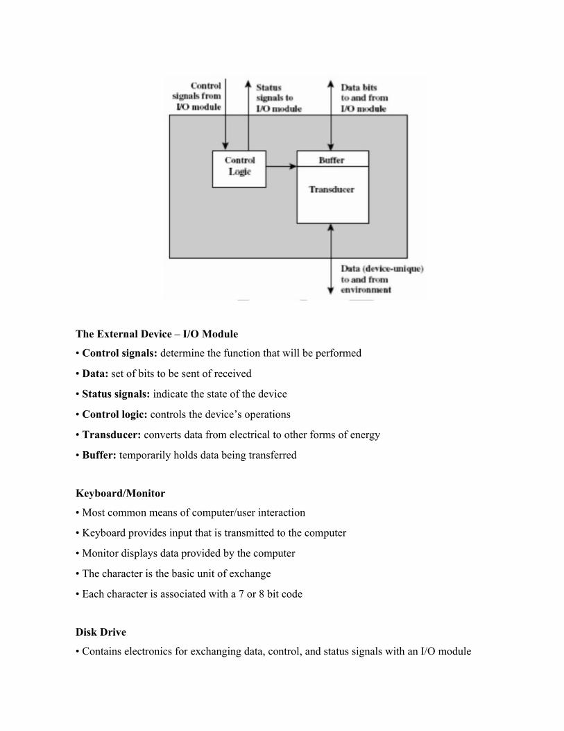
The External Device – I/O Module

• Control signals: determine the function that will be performed

• Data: set of bits to be sent of received

• Status signals: indicate the state of the device

• Control logic: controls the device’s operations

• Transducer: converts data from electrical to other forms of energy

• Buffer: temporarily holds data being transferred

Keyboard/Monitor

• Most common means of computer/user interaction

• Keyboard provides input that is transmitted to the computer

• Monitor displays data provided by the computer

• The character is the basic unit of exchange

• Each character is associated with a 7 or 8 bit code

Disk Drive

• Contains electronics for exchanging data, control, and status signals with an I/O module

• Contains electronics for controlling the disk read/write mechanism

• Fixed-head disk – transducer converts between magnetic patterns on the disk surface and bits

in the buffer

• Moving-head disk – must move the disk arm rapidly across the surface

I/O Modules

Module Function

• Control and timing

• Processor communication

• Device communication

• Data buffering

• Error detection

I/O control steps

• Processor checks I/O module for external device status

• I/O module returns status

• If device ready, processor gives I/O module command to request data transfer

• I/O module gets a unit of data from device

• Data transferred from the I/O module to the processor

Processor communication

Command decoding:

I/O module accepts commands from the processor sent as signals on the control bus

Data:

Data exchanged between the processor and I/O module over the data bus Status reporting:

Common status signals BUSY and READY are used because peripherals are slow

Address recognition:

I/O module must recognize a unique address for each peripheral that it controls I/O module

communication

Device communication:

Commands, status information, and data

Data buffering:

Data comes from main memory in rapid burst and must be buffered by the I/O module and

then sent to the device at the device’s rate

Error detection:

Responsible for reporting errors to the processor

I/O Module Structure: Block Diagram of an I/O Module

Module connects to the computer through a set of signal lines – system bus

• Data transferred to and from the module are buffered with data registers

• Status provided through status registers – may also act as control registers

• Module logic interacts with processor via a set of control signal lines

• Processor uses control signal lines to issue commands to the I/O module

• Module must recognize and generate addresses for devices it controls

• Module contains logic for device interfaces to the devices it controls

• I/O module functions allow the processor to view devices is a simple-minded way

• I/O module may hide device details from the processor so the processor only functions in

terms of simple read and write operations – timing, formats, etc.…

• I/O module may leave much of the work of controlling a device visible to the processor –

rewind a tape, etc.…

I/O channel or I/O processor

• I/O module that takes on most of the detailed processing burden

• Used on mainframe computers

I/O controller of device controller

• Primitive I/O module that requires detailed control

• Used on microcomputers

PROGRAMMED I/O

Overview of Programmed I/O

• Processor executes an I/O instruction by issuing command to appropriate I/O module

• I/O module performs the requested action and then sets the appropriate bits in the I/O status

register – I/O module takes no further action to alert the processor – it does not interrupt the

processor

• The processor periodically checks the status of the I/O module until it determines that the

operation is complete I/O Commands The processor issues an address, specifying I/O module

and device, and an I/O command. The commands are:

• Control: activate a peripheral and tell it what to do

• Test: test various status conditions associated with an I/O module and its peripherals

• Read: causes the I/O module to obtain an item of data from the peripheral and place it into an

internal register

• Write: causes the I/O module to take a unit of data from the data bus

Three Techniques for Input of a Block of Data.

I/O Instructions

Processor views I/O operations in a similar manner as memory operation.

Each device is given a unique identifier or address.

Processor issues commands containing device address – I/O module must check

address lines to see if the command is for itself.

I/O mapping

Memory-mapped I/O Single address space for both memory and I/O devices

Disadvantage

Uses up valuable memory address space

I/O module registers treated as memory addresses

Same machine instructions used to access both memory and I/O devices

Advantage

Allows for more efficient programming

Single read line and single write lines needed

Commonly used

Isolated I/O

Separate address space for both memory and I/O devices

Separate memory and I/O select lines needed

Small number of I/O instructions

Commonly used

DMA (DIRECT MEMORY ACCESS)

DMA Function

• DMA module on system bus used to mimic the processor.

• DMA module only uses system bus when processor does not need it.

• DMA module may temporarily force processor to suspend operations – cycle stealing

DMA Operation

The processor issues a command to DMA module

Read or write

I/O device address using data lines

Starting memory address using data lines – stored in address register

Number of words to be transferred using data lines – stored in data register

The processor then continues with other work

DMA module transfers the entire block of data – one word at a time – directly to or from

memory without going through the processor DMA module sends an interrupt to the processor

when complete

DMA and Interrupt Breakpoints during Instruction Cycle

• The processor is suspended just before it needs to use the bus.

• The DMA module transfers one word and returns control to the processor.

• Since this is not an interrupt the processor does not have to save context.

• The processor executes more slowly, but this is still far more efficient that either programmed

or interrupt-driven I/O.

DMA Configurations

Single bus – detached DMA module each transfer uses bus twice – I/O to DMA, DMA to

memory Processor suspended twice.

Single bus – integrated DMA module

It may support more than one device. Each transfer uses bus once – DMA to memory

Processor suspended once.

Separate I/O bus

Bus supports all DMA enabled devices. Each transfer uses bus once – DMA to memory

Processor suspended once.

INPUT-OUTPUT PROCESSOR (IOP)

Communicate directly with all I/O devices Fetch and execute its own instruction IOP

instructions are specifically designed to facilitate I/O transfer.

Command Instruction that are read form memory by an IOP

Distinguish from instructions that are read by the CPU

Commands are prepared by experienced programmers and are stored in memory

Command word = IOP program Memory

I/O Channels and Processors

The Evolution of the I/O Function

1. Processor directly controls peripheral device

2. Addition of a controller or I/O module – programmed I/O

3. Same as 2 – interrupts added

4. I/O module direct access to memory using DMA

5. I/O module enhanced to become processor like – I/O channel

6. I/O module has local memory of its own – computer like – I/O processor

• More and more the I/O function is performed without processor involvement.

• The processor is increasingly relieved of I/O related tasks – improved performance.

Characteristics of I/O Channels

• Extension of the DMA concept

• Ability to execute I/O instructions – special-purpose processor on I/O channel

– complete control over I/O operations

• Processor does not execute I/O instructions itself – processor initiates I/O transfer by

instructing the I/O channel to execute a program in memory

• Program specifies

Device or devices

Area or areas of memory

Priority

Error condition actions

Two type of I/O channels

Selector channel

Controls multiple high-speed devices

Dedicated to the transfer of data with one of the devices

Each device handled by a controller, or I/O module

I/O channel controls these I/O controllers

Multiplexor channel

Can handle multiple devices at the same time

Byte multiplexor – used for low-speed devices

Block multiplexor – interleaves blocks of data from several devices.

Type of Interfaces

Serial interface – bits transferred one at a time

Parallel interface – multiple bits transferred simultaneously

TEXT / REFERENCE BOOKS

1. M.Morris Mano, ;Computer System Architecture”,Prentice-Hall Publishers,Third Edition.

2. John P Hayes , ‘Computer Architecture and Organization’, McGraw Hill international edition,

Third Edition.

3. Kai Hwang and Faye A Briggs ,‘Computer Architecture and Parallel Processing’, McGraw

Hill international edition,1995.

SCHOOL OF ELECTRICAL AND ELECTRONICS

DEPARTMENT OF ELECTRONICS AND COMMMUNICATION

ENGINEERING

UNIT – IV

COMPUTER ARCHITECTURE AND OPERATING SYSTEM– SCS1315

UNIT.4 INTRODUCTION TO OPERATING SYSTEM

Introduction - Operating system structures - System components - OS services- Process

Management: Processes - Process concepts - Process schedulling-- CPU schedulling

Scheduling algorithms - Preemptive strategies - Non-preemptive strategies.

Operating system structures:

An operating system is a construct that allows the user application programs to interact

with the system hardware. Since the operating system is such a complex structure, it should be

created with utmost care so it can be used and modified easily. An easy way to do this is to create

the operating system in parts. Each of these parts should be well defined with clear inputs, outputs

and functions.

For efficient performance and implementation an OS should be partitioned into separate

subsystems, each with carefully defined tasks, inputs, outputs, and performance characteristics.

These subsystems can then be arranged in various architectural configurations:

Simple Structure

When DOS was originally written its developers had no idea how big and important it

would eventually become. It was written by a few programmers in a relatively short amount of

time, without the benefit of modern software engineering techniques, and then gradually grew over

time to exceed its original expectations. It does not break the system into subsystems, and has no

distinction between user and kernel modes, allowing all programs direct access to the underlying

hardware

MS-DOS layer structure

The original UNIX OS used a simple layered approach, but almost all the OS was in one big

layer, not really breaking the OS down into layered subsystems:

Traditional UNIX system structure

Layered Approach

Another approach is to break the OS into a number of smaller layers, each of which rests

on the layer below it, and relies solely on the services provided by the next lower layer.

This approach allows each layer to be developed and debugged independently, with the

assumption that all lower layers have already been debugged and are trusted to deliver

proper services.

The problem is deciding what order in which to place the layers, as no layer can call upon

the services of any higher layer, and so many chicken-and-egg situations may arise.

Layered approaches can also be less efficient, as a request for service from a higher layer

has to filter through all lower layers before it reaches the HW, possibly with significant

processing at each step.

Layered operating system

Microkernels

The basic idea behind micro kernels is to remove all non-essential services from the kernel,

and implement them as system applications instead, thereby making the kernel as small

and efficient as possible.

Most microkernels provide basic process and memory management, and message passing

between other services, and not much more.

Security and protection can be enhanced, as most services are performed in user mode, not

kernel mode.

System expansion can also be easier, because it only involves adding more system

applications, not rebuilding a new kernel.

Mach was the first and most widely known microkernel, and now forms a major component

of Mac OSX.

Windows NT was originally microkernel, but suffered from performance problems relative

to Windows 95. NT 4.0 improved performance by moving more services into the kernel,

and now XP is back to being more monolithic.

Another microkernel example is QNX, a real-time OS for embedded systems.

Architecture of a typical microkernel

Modules

Modern OS development is object-oriented, with a relatively small core kernel and a set

of modules which can be linked in dynamically. See for example the Solaris structure, as

shown in Figure below.

Modules are similar to layers in that each subsystem has clearly defined tasks and

interfaces, but any module is free to contact any other module, eliminating the problems of

going through multiple intermediary layers, as well as the chicken-and-egg problems.

The kernel is relatively small in this architecture, similar to microkernels, but the kernel

does not have to implement message passing since modules are free to contact each other

directly.

Solaris loadable modules

Hybrid Systems

Most OSes today do not strictly adhere to one architecture, but are hybrids of several.

Mac OS X

The Max OSX architecture relies on the Mach microkernel for basic system management services,

and the BSD kernel for additional services. Application services and dynamically loadable

modules ( kernel extensions ) provide the rest of the OS functionality:

The Mac OS X structure

Operating System Components

These components reflect the services made available by the O.S.

Process Management

Process is a program in execution --- numerous processes to choose from in a

multiprogrammed system,

Process creation/deletion (bookkeeping)

Process suspension/resumption (scheduling, system vs. user)

Process synchronization

Process communication

Deadlock handling

Memory Management

Maintain bookkeeping information

Map processes to memory locations

Allocate/deallocate memory space as requested/required

I/O Device Management

Disk management functions such as free space management, storage allocation,

fragmentation removal, head scheduling

Consistent, convenient software to I/O device interface through buffering/caching,

custom drivers for each device.

File System

Built on top of disk management

File creation/deletion.

Support for hierarchical file systems

Update/retrieval operations: read, write, append, seek

Mapping of files to secondary storage

Protection

Controlling access to the system

Resources --- CPU cycles, memory, files, devices

Users --- authentication, communication

Mechanisms, not policies

Network Management

Often built on top of file system

TCP/IP, IPX, IPng

Connection/Routing strategies

``Circuit'' management --- circuit, message, packet switching

Communication mechanism

Data/Process migration

Network Services (Distributed Computing)

Built on top of networking

Email, messaging (GroupWise)

FTP

gopher, www

Distributed file systems --- NFS, AFS, LAN Manager

Name service --- DNS, YP, NIS

Replication --- gossip, ISIS

Security --- kerberos

User Interface

Character-Oriented shell --- sh, csh, command.com ( User replaceable)

GUI --- X, Windows 95

Operating-System Services

A view of operating system services

OSes provide environments in which programs run, and services for the users of the system,

including:

User Interfaces - Means by which users can issue commands to the system. Depending on

the system these may be a command-line interface ( e.g. sh, csh, ksh, tcsh, etc. ), a GUI

interface ( e.g. Windows, X-Windows, KDE, Gnome, etc. ), or a batch command systems.

The latter are generally older systems using punch cards of job-control language, JCL, but

may still be used today for specialty systems designed for a single purpose.

Program Execution - The OS must be able to load a program into RAM, run the program,

and terminate the program, either normally or abnormally.

I/O Operations - The OS is responsible for transferring data to and from I/O devices,

including keyboards, terminals, printers, and storage devices.

File-System Manipulation - In addition to raw data storage, the OS is also responsible for

maintaining directory and subdirectory structures, mapping file names to specific blocks

of data storage, and providing tools for navigating and utilizing the file system.

Communications - Inter-process communications, IPC, either between processes running

on the same processor, or between processes running on separate processors or separate

machines. May be implemented as either shared memory or message passing, ( or some

systems may offer both. )

Error Detection - Both hardware and software errors must be detected and handled

appropriately, with a minimum of harmful repercussions. Some systems may include

complex error avoidance or recovery systems, including backups, RAID drives, and other

redundant systems. Debugging and diagnostic tools aid users and administrators in tracing

down the cause of problems.

Other systems aid in the efficient operation of the OS itself:

Resource Allocation - E.g. CPU cycles, main memory, storage space, and peripheral

devices. Some resources are managed with generic systems and others with very carefully

designed and specially tuned systems, customized for a particular resource and operating

environment.

Accounting - Keeping track of system activity and resource usage, either for billing

purposes or for statistical record keeping that can be used to optimize future performance.

Protection and Security - Preventing harm to the system and to resources, either through

wayward internal processes or malicious outsiders. Authentication, ownership, and

restricted access are obvious parts of this system. Highly secure systems may log all

process activity down to excruciating detail, and security regulation dictate the storage of

those records on permanent non-erasable medium for extended times in secure ( off-site )

facilities.

Process Management

An OS executes many kinds of activities:

– Users’ programs

– Batch jobs or scripts

– System programs

• Print spoolers, name servers, file servers, network daemons,

• Each of these activities is encapsulated in a process

– A process includes the execution context

• PC, registers, VM, OS resources (e.g., open files), etc…

• Plus the program itself (code and data)

– The OS’s process module manages these processes

• Creation, destruction, scheduling

Program/processor/process

• Note that a program is totally passive

– Just bytes on a disk that encode instructions to be run

• A process is an instance of a program being executed by a

(Real or virtual) processor

– At any instant, there may be many processes running copies of the

Same program (e.g., an editor); each process is separate and (usually) independent

– Linux: ps -auwwx to list all processes

Process operations

• The OS provides the following kinds operations on

Processes (i.e., the process abstraction interface):

– create a process

– delete a process

– suspend a process

– resume a process

– clone a process

– Inter-process communication

– Inter-process synchronization

– create/delete a child process (sub process)

Memory management

• The primary memory is the directly accessed storage for the CPU

– Programs must be stored in memory to execute

– Memory access is fast

– But memory doesn’t survive power failures

• OS must:

– allocate memory space for programs (explicitly and implicitly)

– deallocate space when needed by rest of system

– maintain mappings from physical to virtual memory

• Through page tables

– decide how much memory to allocate to each process

• A policy decision

– decide when to remove a process from memory

• Also policy

I/O

• A big chunk of the OS kernel deals with I/O

– Hundreds of thousands of lines in NT

• The OS provides a standard interface between programs

(User or system) and devices

– file system (disk), sockets (network), frame buffer (video)

• Device drivers are the routines that interact with specific device types

– encapsulates device-specific knowledge

• e.g., how to initialize a device, how to request I/O, how to handle interrupts or errors

• Examples: SCSI device drivers, Ethernet card drivers, video card drivers, sound card drivers

Secondary storage

• Secondary storage (disk, tape) is persistent memory

– Often magnetic media, survives power failures (hopefully)

• Routines that interact with disks are typically at a very low level in the OS

– used by many components (file system, VM …)

– handle scheduling of disk operations, head movement, error handling, and often management

of space on disks

• Usually independent of file system

– Although there may be cooperation

– file system knowledge of device details can help optimize performance

• e.g., place related files close together on disk

File systems

• Secondary storage devices are crude and awkward

– e.g., “write 4096 byte block to sector 12”

• File system: a convenient abstraction

– defines logical objects like files and directories

• hides details about where on disk files live

– As well as operations on objects like read and write

• read/write byte ranges instead of blocks

• A file is the basic unit of long-term storage

– file = named collection of persistent information

• A directory is just a special kind of file

– Directory = named file that contains names of other files and metadata about those files (e.g.,

file size)

File system operations

• The file system interface defines standard operations:

– File (or directory) creation and deletion

– Manipulation of files and directories (read, write, extend, rename, protect)

– Copy

– lock

• File systems also provide higher level services

– Accounting and quotas

– Backup (must be incremental and online!)

– (sometimes) indexing or search

– (sometimes) file versioning

Protection

• Protection is a general mechanism used throughout the OS

– All resources needed to be protected

• Memory

• Processes

• Files

• Devices

• CPU time

– Protection mechanisms help to detect and contain unintentional errors, as well as preventing

malicious destruction

Command interpreter (shell)

• A particular program that handles the interpretation of users’ commands and helps to manage

processes

– User input may be from keyboard (command-line interface), from script files, or from the

mouse (GUIs)

– allows users to launch and control new programs

• On some systems, command interpreter may be a standard part of the OS (e.g., MS DOS,

Apple II)

• On others, it’s just non-privileged code that provides an interface to the user

– e.g., bash/csh/tcsh/zsh on UNIX

• On others, there may be no command language

– e.g., MacOS

Process Scheduling

The act of determining which process is in the ready state, and should be moved to the running

state is known as Process Scheduling.

The prime aim of the process scheduling system is to keep the CPU busy all the time and to

deliver minimum response time for all programs. For achieving this, the scheduler must apply

appropriate rules for swapping processes IN and OUT of CPU.

Scheduling fell into one of the two general categories:

Non Pre-emptive Scheduling: When the currently executing process gives up the CPU

voluntarily.

Pre-emptive Scheduling: When the operating system decides to favour another process, pre-

empting the currently executing process.

Scheduling Queues

All processes, upon entering into the system, are stored in the Job Queue.

Processes in the Ready state are placed in the Ready Queue.

Processes waiting for a device to become available are placed in Device Queues. There are unique

device queues available for each I/O device.

A new process is initially put in the Ready queue. It waits in the ready queue until it is selected for

execution (or dispatched). Once the process is assigned to the CPU and is executing, one of the

following several events can occur:

The process could issue an I/O request, and then be placed in the I/O queue.

The process could create a new sub process and wait for its termination.

The process could be removed forcibly from the CPU, as a result of an interrupt, and be

put back in the ready queue.

Scheduling Queues figure

In the first two cases, the process eventually switches from the waiting state to the ready state,

and is then put back in the ready queue. A process continues this cycle until it terminates, at

which time it is removed from all queues and has its PCB and resources deallocated.

Types of Schedulers

There are three types of schedulers available:

Long Term Scheduler

Short Term Scheduler

Medium Term Scheduler

Let's discuss about all the different types of Schedulers in detail:

Long Term Scheduler

Long term scheduler runs less frequently. Long Term Schedulers decide which program must get

into the job queue. From the job queue, the Job Processor, selects processes and loads them into

the memory for execution. Primary aim of the Job Scheduler is to maintain a good degree of

Multiprogramming. An optimal degree of Multiprogramming means the average rate of process

creation is equal to the average departure rate of processes from the execution memory.

Short Term Scheduler

This is also known as CPU Scheduler and runs very frequently. The primary aim of this

scheduler is to enhance CPU performance and increase process execution rate.

Medium Term Scheduler

This scheduler removes the processes from memory (and from active contention for the CPU),

and thus reduces the degree of multiprogramming. At some later time, the process can be

reintroduced into memory and its execution van be continued where it left off. This scheme is

called swapping. The process is swapped out, and is later swapped in, by the medium term

scheduler.

Swapping may be necessary to improve the process mix, or because a change in memory

requirements has overcommitted available memory, requiring memory to be freed up. This

complete process is descripted in the below diagram:

Context Switch

Switching the CPU to another process requires saving the state of the old process and

loading the saved state for the new process. This task is known as a Context Switch.

The context of a process is represented in the Process Control Block (PCB) of a process;

it includes the value of the CPU registers, the process state and memory-management

information. When a context switch occurs, the Kernel saves the context of the old

process in its PCB and loads the saved context of the new process scheduled to run.

Context switch time is pure overhead, because the system does no useful work while

switching. Its speed varies from machine to machine, depending on the memory speed,

the number of registers that must be copied, and the existence of special instructions

(such as a single instruction to load or store all registers). Typical speeds range from 1 to

1000 microseconds.

Context Switching has become such a performance bottleneck that programmers are

using new structures (threads) to avoid it whenever and wherever possible.

CPU Scheduling

CPU scheduling is a process which allows one process to use the CPU while the execution of

another process is on hold (in waiting state) due to unavailability of any resource like I/O etc.,

thereby making full use of CPU. The aim of CPU scheduling is to make the system efficient, fast

and fair.

Whenever the CPU becomes idle, the operating system must select one of the processes in the

ready queue to be executed. The selection process is carried out by the short-term scheduler (or

CPU scheduler). The scheduler selects from among the processes in memory that are ready to

execute, and allocates the CPU to one of them.

Types of CPU Scheduling

CPU scheduling decisions may take place under the following four circumstances:

When a process switches from the running state to the waiting state (for I/O request or

invocation of wait for the termination of one of the child processes).

When a process switches from the running state to the ready state (for example, when an

interrupt occurs).

When a process switches from the waiting state to the ready state (for example,

completion of I/O).

When a process terminates.

In circumstances 1 and 4, there is no choice in terms of scheduling. A new process (if one exists

in the ready queue) must be selected for execution. There is a choice, however in circumstances

2 and 3.

When Scheduling takes place only under circumstances 1 and 4, we say the scheduling scheme is

non-preemptive; otherwise the scheduling scheme is preemptive.

Non-Preemptive Scheduling

Under non-preemptive scheduling, once the CPU has been allocated to a process, the process

keeps the CPU until it releases the CPU either by terminating or by switching to the waiting

state.

This scheduling method is used by the Microsoft Windows 3.1 and by the Apple Macintosh

operating systems.

It is the only method that can be used on certain hardware platforms, because It does not require

the special hardware (for example: a timer) needed for preemptive scheduling.

Preemptive Scheduling

In this type of Scheduling, the tasks are usually assigned with priorities. At times it is necessary

to run a certain task that has a higher priority before another task although it is running.

Therefore, the running task is interrupted for some time and resumed later when the priority task

has finished its execution.

Below are different time with respect to a process.

Arrival Time: Time at which the process arrives in the ready queue.

Completion Time: Time at which process completes its execution.

Burst Time: Time required by a process for CPU execution.

Turn Around Time: Time Difference between completion time and arrival time.

Turn Around Time = Completion Time – Arrival Time

Waiting Time (W.T): Time Difference between turnaround time and burst time.

Waiting Time = Turn Around Time – Burst Time

Scheduling Algorithms

To decide which process to execute first and which process to execute last to achieve maximum

CPU utilization, computer scientists have defined some algorithms, and they are:

First Come First Serve(FCFS) Scheduling

Shortest-Job-First(SJF) Scheduling

Priority Scheduling

Round Robin(RR) Scheduling

Multilevel Queue Scheduling

Multilevel Feedback Queue Scheduling

First Come First Serve (FCFS)

Jobs are executed on first come, first serve basis.

It is a non-preemptive, pre-emptive scheduling algorithm.

Easy to understand and implement.

Its implementation is based on FIFO queue.

Poor in performance as average wait time is high.

Wait time of each process is as follows –

Average Wait Time: (0+4+6+13) / 4 = 5.75

Shortest Job Next (SJN)

This is also known as shortest job first, or SJF

This is a non-preemptive, pre-emptive scheduling algorithm.

Best approach to minimize waiting time.

Easy to implement in Batch systems where required CPU time is known in advance.

Impossible to implement in interactive systems where required CPU time is not known.

The processer should know in advance how much time process will take.

Given: Table of processes, and their Arrival time, Execution time

Waiting time of each process is as follows –

Average Wait Time: (0 + 4 + 12 + 5)/4 = 21 / 4 = 5.25

Priority Based Scheduling

Priority scheduling is a non-preemptive algorithm and one of the most common

scheduling algorithms in batch systems.

Each process is assigned a priority. Process with highest priority is to be executed first

and so on.

Processes with same priority are executed on first come first served basis.

Priority can be decided based on memory requirements, time requirements or any other

resource requirement.

Given: Table of processes, and their Arrival time, Execution time, and priority. Here we are

considering 1 is the lowest priority.

Waiting time of each process is as follows –

Average Wait Time: (0 + 10 + 12 + 2)/4 = 24 / 4 = 6

Shortest Remaining Time

Shortest remaining time (SRT) is the preemptive version of the SJN algorithm.

The processor is allocated to the job closest to completion but it can be preempted by a

newer ready job with shorter time to completion.

Impossible to implement in interactive systems where required CPU time is not known.

It is often used in batch environments where short jobs need to give preference.

Round Robin Scheduling

Round Robin is the preemptive process scheduling algorithm.

Each process is provided a fix time to execute, it is called a quantum.

Once a process is executed for a given time period, it is preempted and other process

executes for a given time period.

Context switching is used to save states of preempted processes.

Wait time of each process is as follows –

Average Wait Time: (9+2+12+11) / 4 = 8.5

Multiple-Level Queues Scheduling

Multiple-level queues are not an independent scheduling algorithm. They make use of

other existing algorithms to group and schedule jobs with common characteristics.

Multiple queues are maintained for processes with common characteristics.

Each queue can have its own scheduling algorithms.

Priorities are assigned to each queue.

For example, CPU-bound jobs can be scheduled in one queue and all I/O-bound jobs in another

queue. The Process Scheduler then alternately selects jobs from each queue and assigns them to

the CPU based on the algorithm assigned to the queue.

Multilevel feedback queue scheduler is defined by the following parameters:

The number of queues.

The scheduling algorithm for each queue.

The method used to determine when to upgrade a process to a higher-priority queue.

The method used to determine when to demote a process to a lower-priority queue.

The method used to determine which queue a process will enter when that process needs

service.

TEXT / REFERENCE BOOKS

1. Abraham Silberschatz,Peter Galvin and Gagne, “Operating System Concepts”, 6th Edition,

Addison Wesley, 2002.

2. Harvey M.Deitel, ”Operating System”, 2nd Edition, Addison Wesley, 2000.

SCHOOL OF ELECTRICAL AND ELECTRONICS

DEPARTMENT OF ELECTRONICS AND COMMMUNICATION ENGINEERING

UNIT – V

COMPUTER ARCHITECTURE AND OPERATING SYSTEM– SCS1315

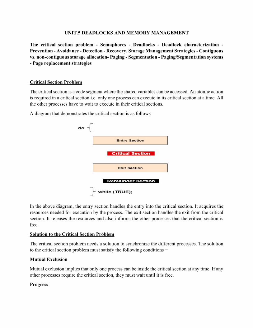
UNIT.5 DEADLOCKS AND MEMORY MANAGEMENT

The critical section problem - Semaphores - Deadlocks - Deadlock characterization - Prevention - Avoidance - Detection - Recovery. Storage Management Strategies - Contiguous vs. non-contiguous storage allocation- Paging - Segmentation - Paging/Segmentation systems - Page replacement strategies

Critical Section Problem

The critical section is a code segment where the shared variables can be accessed. An atomic action is required in a critical section i.e. only one process can execute in its critical section at a time. All the other processes have to wait to execute in their critical sections.

A diagram that demonstrates the critical section is as follows –

In the above diagram, the entry section handles the entry into the critical section. It acquires the resources needed for execution by the process. The exit section handles the exit from the critical section. It releases the resources and also informs the other processes that the critical section is free.

Solution to the Critical Section Problem

The critical section problem needs a solution to synchronize the different processes. The solution to the critical section problem must satisfy the following conditions −

Mutual Exclusion

Mutual exclusion implies that only one process can be inside the critical section at any time. If any other processes require the critical section, they must wait until it is free.

Progress

Progress means that if a process is not using the critical section, then it should not stop any other process from accessing it. In other words, any process can enter a critical section if it is free.

Bounded Waiting

Bounded waiting means that each process must have a limited waiting time. It should not wait endlessly to access the critical section.

Semaphores

Semaphores are integer variables that are used to solve the critical section problem by using two atomic operations, wait and signal that are used for process synchronization.

The definitions of wait and signal are as follows −

Wait

The wait operation decrements the value of its argument S, if it is positive. If S is negative or zero, then no operation is performed.

wait(S)

{

while (S<=0);

S--;

}

Signal

The signal operation increments the value of its argument S.

signal(S)

{

S++;

}

Types of Semaphores

There are two main types of semaphores i.e. counting semaphores and binary semaphores. Details about these are given as follows −

Counting Semaphores

These are integer value semaphores and have an unrestricted value domain. These semaphores are used to coordinate the resource access, where the semaphore count is the number of available

resources. If the resources are added, semaphore count automatically incremented and if the resources are removed, the count is decremented.

Binary Semaphores

The binary semaphores are like counting semaphores but their value is restricted to 0 and 1. The wait operation only works when the semaphore is 1 and the signal operation succeeds when semaphore is 0. It is sometimes easier to implement binary semaphores than counting semaphores.

Advantages of Semaphores

Some of the advantages of semaphores are as follows −

Semaphores allow only one process into the critical section. They follow the mutual exclusion principle strictly and are much more efficient than some other methods of synchronization.

There is no resource wastage because of busy waiting in semaphores as processor time is not wasted unnecessarily to check if a condition is fulfilled to allow a process to access the critical section.

Semaphores are implemented in the machine independent code of the microkernel. So they are machine independent.

Disadvantages of Semaphores

Some of the disadvantages of semaphores are as follows −

Semaphores are complicated so the wait and signal operations must be implemented in the correct order to prevent deadlocks.

Semaphores are impractical for last scale use as their use leads to loss of modularity. This happens because the wait and signal operations prevent the creation of a structured layout for the system.

Semaphores may lead to a priority inversion where low priority processes may access the critical section first and high priority processes later.

Deadlocks

Deadlock is a situation where a set of processes are blocked because each process is holding a resource and waiting for another resource acquired by some other process.

A process in operating systems uses different resources and uses resources in the following way.

Requests a resource Use the resource Releases the resource

In the above diagram, the process 1 has resource 1 and needs to acquire resource 2. Similarly process 2 has resource 2 and needs to acquire resource 1. Process 1 and process 2 are in deadlock as each of them needs the other’s resource to complete their execution but neither of them is willing to relinquish their resources.

Deadlock can arise if the following four conditions hold simultaneously (Necessary Conditions)

Mutual Exclusion: One or more than one resource are non-shareable (Only one process can use at a time)

Hold and Wait: A process is holding at least one resource and waiting for resources. No Preemption: A resource cannot be taken from a process unless the process releases the

resource. Circular Wait: A set of processes are waiting for each other in circular form.

A deadlock occurs if the four Coffman conditions hold true. But these conditions are not mutually exclusive. They are given as follows –

Mutual Exclusion

There should be a resource that can only be held by one process at a time. In the diagram below, there is a single instance of Resource 1 and it is held by Process 1 only.

Hold and Wait

A process can hold multiple resources and still request more resources from other processes which are holding them. In the diagram given below, Process 2 holds Resource 2 and Resource 3 and is requesting the Resource 1 which is held by Process 1.

No Preemption

A resource cannot be preempted from a process by force. A process can only release a resource voluntarily. In the diagram below, Process 2 cannot preempt Resource 1 from Process 1. It will only be released when Process 1 relinquishes it voluntarily after its execution is complete.

Circular Wait

A process is waiting for the resource held by the second process, which is waiting for the resource held by the third process and so on, till the last process is waiting for a resource held by the first process. This forms a circular chain. For example: Process 1 is allocated Resource2 and it is requesting Resource 1. Similarly, Process 2 is allocated Resource 1 and it is requesting Resource 2. This forms a circular wait loop.

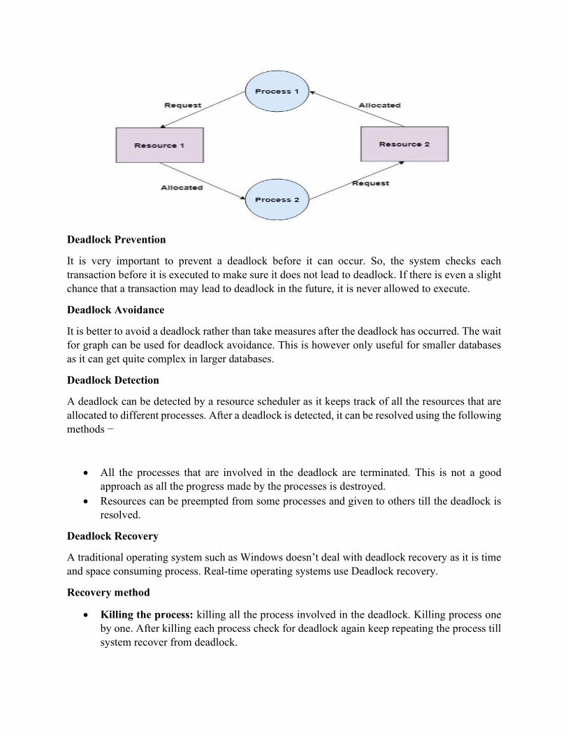
Deadlock Prevention

It is very important to prevent a deadlock before it can occur. So, the system checks each transaction before it is executed to make sure it does not lead to deadlock. If there is even a slight chance that a transaction may lead to deadlock in the future, it is never allowed to execute.

Deadlock Avoidance

It is better to avoid a deadlock rather than take measures after the deadlock has occurred. The wait for graph can be used for deadlock avoidance. This is however only useful for smaller databases as it can get quite complex in larger databases.

Deadlock Detection

A deadlock can be detected by a resource scheduler as it keeps track of all the resources that are allocated to different processes. After a deadlock is detected, it can be resolved using the following methods −

All the processes that are involved in the deadlock are terminated. This is not a good approach as all the progress made by the processes is destroyed.

Resources can be preempted from some processes and given to others till the deadlock is resolved.

Deadlock Recovery

A traditional operating system such as Windows doesn’t deal with deadlock recovery as it is time and space consuming process. Real-time operating systems use Deadlock recovery.

Recovery method

Killing the process: killing all the process involved in the deadlock. Killing process one by one. After killing each process check for deadlock again keep repeating the process till system recover from deadlock.

Resource Preemption: Resources are preempted from the processes involved in the deadlock, preempted resources are allocated to other processes so that there is a possibility of recovering the system from deadlock. In this case, the system goes into starvation.

Storage Management

Storage Management is defined as it refers to the management of the data storage equipment’s that are used to store the user/computer generated data.

Storage management key attributes:

Storage management has some key attribute which is generally used to manage the storage capacity of the system. These are given below:

Performance Reliability Recoverability Capacity

Feature of Storage management:

There is some feature of storage management which is provided for storage capacity. These are given below:

Storage management is a process that is used to optimize the use of storage devices. Storage management must be allocated and managed as a resource in order to truly benefit

a corporation. Storage management is generally a basic system component of information systems. It is used to improve the performance of their data storage resources.

Advantage of storage management:

There are some advantage of storage management which are given below:

It is very simple to manage a storage capacity. It is generally take a less time. It is improve the performance of system. In virtualization and automation technologies can help an organization improve its agility.

Memory management

Memory is central to the operation of a computer system. It consists of a large array of words or bytes each with its own address.

Memory management techniques

The memory management techniques is divided into two parts...

Uniprogramming:

In the uni-programming technique, the RAM is divided into two parts one part is for the resigning the operating system and other portion is for the user process. Here the fence register is used which contain the last address of the operating system parts. The operating system will compare the user data addresses with the fence register and if it is different that means the user is not entering in the OS area. Fence register is also called boundary register and is used to prevent a user from entering in the operating system area. Here the CPU utilization is very poor and hence multiprogramming is used.

Multiprogramming:

In the multiprogramming, the multiple users can share the memory simultaneously. By multiprogramming we mean there will be more than one process in the main memory and if the running process wants to wait for an event like I/O then instead of sitting ideal CPU will make a context switch and will pick another process.

Contiguous memory allocation Non-contiguous memory allocation

a) Contiguous memory allocation

In contiguous memory allocation, all the available memory space remain together in one place. It means freely available memory partitions are not scattered here and there across the whole memory space.

In the contiguous memory allocation, both the operating system and the user must reside in the main memory. The main memory is divided into two portions one portion is for the operating and other is for the user program.

In the contiguous memory allocation when any user process request for the memory a single section of the contiguous memory block is given to that process according to its need. We can achieve contiguous memory allocation by dividing memory into the fixed-sized partition.

A single process is allocated in that fixed sized single partition. But this will increase the degree of multiprogramming means more than one process in the main memory that bounds the number of fixed partition done in memory. Internal fragmentation increases because of the contiguous memory allocation.

Fixed sized partition

In the fixed sized partition the system divides memory into fixed size partition (may or may not be of the same size) here entire partition is allowed to a process and if there is some wastage inside the partition is allocated to a process and if there is some wastage inside the partition then it is called internal fragmentation.

Advantage: Management or book keeping is easy.

Disadvantage: Internal fragmentation

Variable size partition

In the variable size partition, the memory is treated as one unit and space allocated to a process is exactly the same as required and the leftover space can be reused again.

Advantage: There is no internal fragmentation.

Disadvantage: Management is very difficult as memory is becoming purely fragmented after some time.

b) Non-contiguous memory allocation

In the non-contiguous memory allocation the available free memory space are scattered here and there and all the free memory space is not at one place. So this is time-consuming. In the non-contiguous memory allocation, a process will acquire the memory space but it is not at one place it is at the different locations according to the process requirement. This technique of non-contiguous memory allocation reduces the wastage of memory which leads to internal and external fragmentation. This utilizes all the free memory space which is created by a different process.

Non-contiguous memory allocation is of different types,

Paging Segmentation Segmentation with paging

i) Paging

A non-contiguous policy with a fixed size partition is called paging. A computer can address more memory than the amount of physically installed on the system. This extra memory is actually called virtual memory. Paging technique is very important in implementing virtual memory. Secondary memory is divided into equal size partition (fixed) called pages. Every process will have a separate page table. The entries in the page table are the number of pages a process. At each entry either we have an invalid pointer which means the page is not in main memory or we will get the corresponding frame number. When the frame number is combined with instruction of set D than we will get the corresponding physical address. Size of a page table is generally very large so cannot be accommodated inside the PCB, therefore, PCB contains a register value PTBR (page table base register) which leads to the page table.

A computer can address more memory than the amount physically installed on the system. This extra memory is actually called virtual memory and it is a section of a hard that's set up to emulate the computer's RAM. Paging technique plays an important role in implementing virtual memory.

Paging is a memory management technique in which process address space is broken into blocks of the same size called pages (size is power of 2, between 512 bytes and 8192 bytes). The size of the process is measured in the number of pages.

Similarly, main memory is divided into small fixed-sized blocks of (physical) memory called frames and the size of a frame is kept the same as that of a page to have optimum utilization of the main memory and to avoid external fragmentation.

Address Translation

Page address is called logical address and represented by page number and the offset. Logical Address = Page number + page offset Frame address is called physical address and represented by a frame number and the offset. Physical Address = Frame number + page offset A data structure called page map table is used to keep track of the relation between a pages

of a process to a frame in physical memory.

When the system allocates a frame to any page, it translates this logical address into a physical address and create entry into the page table to be used throughout execution of the program.

When a process is to be executed, its corresponding pages are loaded into any available memory frames. Suppose you have a program of 8Kb but your memory can accommodate only 5Kb at a given point in time, then the paging concept will come into picture. When a computer runs out of RAM, the operating system (OS) will move idle or unwanted pages of memory to secondary memory to free up RAM for other processes and brings them back when needed by the program.

This process continues during the whole execution of the program where the OS keeps removing idle pages from the main memory and write them onto the secondary memory and bring them back when required by the program.

Advantages: It is independent of external fragmentation.

Disadvantages:

It makes the translation very slow as main memory access two times. A page table is a burden over the system which occupies considerable space.

ii) Segmentation

Segmentation is a programmer view of the memory where instead of dividing a process into equal size partition we divided according to program into partition called segments. The translation is the same as paging but paging segmentation is independent of internal fragmentation but suffers from external fragmentation. Reason of external fragmentation is program can be divided into segments but segment must be contiguous in nature.

iii) Segmentation with paging

In segmentation with paging, we take advantages of both segmentation as well as paging. It is a kind of multilevel paging but in multilevel paging, we divide a page table into equal size partition

but here in segmentation with paging, we divide it according to segments. All the properties are the same as that of paging because segments are divided into pages.

Page Replacement Strategies

In an operating system that uses paging for memory management, a page replacement algorithm is needed to decide which page needs to be replaced when new page comes in.

Page Fault – A page fault happens when a running program accesses a memory page that is mapped into the virtual address space, but not loaded in physical memory.

Page Replacement Algorithms:

FIFO Page Replacement Algorithm-

As the name suggests, this algorithm works on the principle of “First in First out“. It replaces the oldest page that has been present in the main memory for the longest time. It is implemented by keeping track of all the pages in a queue.

LIFO Page Replacement Algorithm-

As the name suggests, this algorithm works on the principle of “Last in First out“. It replaces the newest page that arrived at last in the main memory. It is implemented by keeping track of all the pages in a stack.

NOTE

Only frame is used for page replacement during entire procedure after all the frames get occupied.

LRU Page Replacement Algorithm-

As the name suggests, this algorithm works on the principle of “Least Recently Used“.

It replaces the page that has not been referred by the CPU for the longest time.

Optimal Page Replacement Algorithm-

This algorithm replaces the page that will not be referred by the CPU in future for the longest time.

It is practically impossible to implement this algorithm. This is because the pages that will not be used in future for the longest time cannot be

predicted. However, it is the best known algorithm and gives the least number of page faults. Hence, it is used as a performance measure criterion for other algorithms.

Random Page Replacement Algorithm-

As the name suggests, this algorithm randomly replaces any page. So, this algorithm may behave like any other algorithm like FIFO, LIFO, LRU, Optimal

etc.

TEXT / REFERENCE BOOKS

1. Abraham Silberschatz,Peter Galvin and Gagne, “Operating System Concepts”, 6th Edition,

Addison Wesley, 2002.

2. Harvey M.Deitel, ”Operating System”, 2nd Edition, Addison Wesley, 2000.