The Value of “New” and “Old” Intermediationin Online Debt Crowdfunding

Fabio Braggion Alberto Manconi Nicola Pavanini

Haikun Zhu*

December 2020

AbstractWe study the welfare effects of the transition of online debt crowdfundingfrom the older “peer-to-peer” model to the “marketplace” model, where thecrowdfunding platform sells diversified loan portfolios to investors. We de-velop an equilibrium model of debt crowdfunding and estimate it on a noveldatabase from a large Chinese platform. Moving from the peer-to-peer to themarketplace model raises lender surplus, platform profits, and credit provi-sion. Moreover, reducing lender exposure to liquidity risk can be beneficial.A counterfactual where the platform resembles a bank by bearing liquidityrisk generates larger lender surplus and credit provision when liquidity is low.

JEL classification: D14, D61, G21, G51, L21Keywords: Marketplace credit, Chinese financial system, Structural estima-tion

*Braggion: Tilburg University, CEPR and ECGI, f.braggion@tilburguniversity.edu; Manconi:Bocconi University and CEPR, alberto.manconi@unibocconi.it; Pavanini: Tilburg University andCEPR, n.pavanini@tilburguniversity.edu; Zhu: ESE Rotterdam, h.zhu@ese.eur.nl. We thank Mat-teo Benetton, Chiara Farronato, Jean-François Houde, Yi Huang, Emiliano Pagnotta, Stefano Sac-chetto, Lei Xu, as well as seminar and conference participants at University of Zürich, McGill Uni-versity, 2019 Conference on Regulating Financial Markets, Graduate Institute Geneva, LUISS, 7th

Workshop in Macro Banking and Finance (Collegio Carlo Alberto), University of Rochester SimonSchool of Business, 2020 TSE Digital Economics Conference, HEC Paris, 2020 Stanford Institutefor Theoretical Economics Summer Workshop on Financial Regulation, Tilburg Economics, BPI-Fundação La Caixa-Nova 2020 FinTech Conference, University of Michigan, University of Vienna,Cornell-Wisconsin IO seminar.

1

1 Introduction

Online debt crowdfunding is an increasingly important investment and consumercredit channel. Averaging yearly growth rates well above 100%, the segment hasreached $284 bn in outstanding loans in 2016 (Rau 2019). Debt crowdfunding hasmoved from an older “peer-to-peer” model, where lenders pick the individual loansthey fund, to a “marketplace” model, where the crowdfunding platform sells loanportfolio products to lenders (Balyuk and Davydenko 2019, Vallée and Zeng 2019).That has brought platforms closer to traditional banks, in that portfolio products areshorter-term liabilities invested in longer-term loans. Unlike bank depositors, how-ever, marketplace lenders bear liquidity risk: they can only cash out their investmentonce the underlying loans are sold on the platform’s secondary market.

We study the effects of the new business model on lenders, platforms, and creditprovision. We develop an equilibrium model of debt crowdfunding capturing plat-form design (peer-to-peer, marketplace) and lender preferences over loan and port-folio product characteristics, and we estimate it on a novel database on credit at alarge online platform. We find that moving from the peer-to-peer to the market-place model raises lender surplus, platform profits, and credit provision. At thesame time, reducing lender exposure to liquidity risk can be beneficial. A counter-factual scenario where the platform resembles a bank by bearing liquidity risk hassimilar welfare effects as the marketplace model when liquidity is high and lenderliquidity risk–aversion moderate, but improves welfare when liquidity is low andrisk aversion higher.

Our analysis is motivated by the observation that a welfare comparison betweenmarketplace, peer-to-peer, and traditional bank credit is not obvious. Marketplacelenders are exposed to liquidity risk; but compared to peer-to-peer lenders, they facelower search, diversification, and adverse selection costs; and compared to bankdepositors they earn higher returns. In turn, lowering costs and increasing returnsfor lenders, as well as shielding the platform from liquidity risk, incentivize creditprovision, benefiting borrowers. Quantifying these tradeoffs is crucial to informregulation and to address growing concerns about liquidity risk on online credit

2

platforms (BIS 2017).1 Thus, we must assess the costs and benefits of alternativeplatform designs on the data.

Measuring those costs and benefits, however, confronts us with three empiri-cal challenges. First, it requires counterfactuals. The ideal experiment comparesoutcomes for otherwise identical platforms under the marketplace model, the peer-to-peer model, and a bank-like version of the marketplace model where the platformbears liquidity risk. But little peer-to-peer credit exists any longer, and no platformadopted the bank-like model as yet—and if one were to introduce it, its launchwould not be randomly assigned.2 Second, the main difference between alternativeplatform designs is how large is liquidity risk and who bears it. But liquidity riskarises from a misalignment between lender, platform, and borrower horizons, sothat micro data are necessary to draw the link between a lender’s investments andthe loans that the platform originates to borrowers. Third, the welfare impact ofplatform design depends on how lender preferences trade off expected return andliquidity risk. But those preferences are intrinsically unobservable, challenging toidentify, and evolving as marketplace credit reaches a larger, more heterogeneousinvestor pool.

We address these challenges with a structural estimation approach and withnovel data. First, we build a model of online credit following the industrial or-ganization literature on demand estimation for differentiated products (Berry 1994,Berry, Levinsohn and Pakes 1995). The model nests the marketplace, peer-to-peer,and bank-like platform designs, allowing us to simulate counterfactual scenariosand compare their welfare effects. Second, we estimate the model and base ouranalysis on a new, hand-collected micro database covering the universe of loansand loan applications on Renrendai (人人贷), a leading Chinese debt crowdfundingplatform. We observe the composition of portfolio products, and we can comparetheir maturities to those of the underlying loans in order to quantify liquidity risk.

1These concerns have also been voiced in the press, see e.g. “Peer-to-peer lending needs tighterregulation,” Financial Times 11 September 2018; “China curbs ‘Wild West’ P2P loan sector,” Finan-cial Times 5 April 2017, and “Funding Circle seeks to ease fears over withdrawal delays,” FinancialTimes 11 October 2019.

2As a first-ever case, Zopa was granted a full U.K. banking license in December 2018 and hasplanned the introduction of fixed-term savings accounts (“P2P Lender Zopa Granted Full UK Ban-king License,” Financial Times 4 December 2018).

3

Third, the model recovers lender preferences from observed investment choices,providing a measure of surplus and a way to account for lender heterogeneity in ourcounterfactuals. Moreover, we have access to the entire information set observedby the lenders, attenuating the possibility that any omitted variables may bias theestimates of the lenders’ preference parameters.

Our main findings are as follows. First, we observe a transition to marketplacecredit: in 2010, when Renrendai was launched, 100% of lending was peer-to-peer;by the end of our sample in early 2017, over 98% was marketplace. Our data indi-cate that this trend may have given rise to non-trivial liquidity risk: whereas most ofRenrendai’s portfolio products have maturities of 3, 6, or 12 months, the underlyingloans typically mature in 36 months. Moreover, lender investments have becomemore diversified and less exposed to defaults, especially so for portfolio productspurchased on the platform, consistent with a change in the platform’s clientele to-wards investors more averse to risk.

Second, the estimates of our structural model shed light on lender preferencesfor loan and portfolio product characteristics, as well as on the platform’s prefe-rences for individual loan attributes. Lenders prefer higher returns, especially forpeer-to-peer loans, and portfolio products with lower liquidity risk, measured interms of resale time on the secondary market. Moreover, the lenders’ preferencesare heterogeneous: the more sophisticated, active lenders have a stronger prefe-rence for yield and a weaker disutility from liquidity risk, whereas the opposite istrue for less frequent investors. We interpret this as evidence that lenders with moreappetite for yield might benefit from the marketplace model, while others, moreconcerned about liquidity risk, might be better off under the bank-like model. Wealso find that Renrendai prefers to include longer-maturity, low-yield loans in itsportfolio products. That is consistent with an attempt to reduce adverse selectionby avoiding the riskier borrowers, in line with Stiglitz and Weiss (1981); but at thesame time, it may exacerbate the maturity mismatch with the portfolio products,which have shorter maturities.

Third, we combine our estimates of the lender demand model with a platformprofit function to simulate counterfactuals. We compare the baseline marketplacecredit with two counterfactual scenarios: peer-to-peer credit, where only direct

4

lending is allowed, and bank-like credit, where the platform sells portfolio productsbut bears liquidity risk. In the marketplace and bank-like scenarios, the platformmaximizes profits by choosing portfolio product target return and the mismatch be-tween portfolio duration and the maturity of the underlying loans. The marketplacemodel appears welfare-improving relative to the peer-to-peer model: the counter-factual allowing only direct lending generates a 65% drop in credit provision and a55% decline in lender surplus. We also find that, with a baseline level of liquidity(time to loan resale around half a day), bank-like credit results in identical loanvolumes and lender surplus as marketplace credit, and a minimal drop in platformprofits (0.2%).

That comparison is different, however, under a “stress test” scenario where weraise the time to loan resale to one month.3 Under that scenario, relative to thebank-like model the marketplace model exhibits a larger decline in credit provision(8% vs 1%) and lender surplus (34% vs 0.5%), but a smaller drop in platform pro-fits (9% vs 12%). In other words, when liquidity is low the marketplace model ispreferable from the platform’s point of view, but worse for lenders and borrowers.The potential conflict between the interests of the platform, lenders, and borrowersmight reflect the current reach of online debt crowdfunding and the features of thelender population. When, in a final counterfactual, we alter the lenders’ composi-tion to have weaker utility from yield and stronger disutility from liquidity risk onaverage, we find that the bank-like model is a Pareto improvement, raising platformprofits too.

Our paper makes three main contributions. First, it provides new results on thedesign of online debt crowdfunding platforms. The literature has looked at adverseselection costs (Vallée and Zeng 2019) and pricing mechanisms (Franks, Serrano-Velarde and Sussman 2020) in online lending. We take a different, complementaryangle. Building on the evidence of the shift to marketplace, or reintermediation(Balyuk and Davydenko 2019), we focus on liquidity risk and on measuring the

3Although much longer than the baseline scenario, that is well within the range experienced bylenders on Renrendai (the maximum time to resale we observe is 88 days). It is also significantly lessthan the four months resale time observed on Funding Circle, the largest U.K. debt crowdfundingplatform, in 2019 (“Funding Circle seeks to ease fears over withdrawal delays,” Financial Times, 11October 2019).

5

welfare value of alternative platform designs. In that respect we also relate to theliterature comparing online and traditional credit intermediaries (Buchak, Matvos,Piskorski and Seru 2018, de Roure, Pelizzon and Thakor 2019), as well as to theindustrial organization literature on online marketplaces reviewed by Einav, Far-ronato and Levin (2016). Our results help rationalize the evolution of platform de-sign from peer-to-peer to marketplace, and provide insight into its potential futuredevelopment in light of the comparison with the bank-like model.

Second, our paper contributes to the literature on structural estimation in fi-nancial intermediation (Egan, Hortaçsu and Matvos 2017, Crawford, Pavanini andSchivardi 2018), online credit (Kawai, Onishi and Uetake 2016, Xin 2018, Tang2020), and online marketplaces in general (Dinerstein, Einav, Levin and Sundare-san 2018, Einav, Farronato, Levin and Sundaresan 2018, Fréchette, Lizzeri and Salz2019, Farronato and Fradkin 2018). Work in this literature has so far focused onbuyers and sellers or lenders and borrowers, leaving aside an active role for plat-forms. In contrast, our approach directly models the design of portfolio productsby the platform. This is central to our arguments and empirically relevant, as itreflects the recent shift of online debt crowdfunding from the peer-to-peer to themarketplace paradigm.

Third, our paper contributes to the literature on the value of financial interme-diation. Theory work has emphasized the role of intermediaries such as banks infacilitating the provision of credit for longer-term projects via maturity transfor-mation (Diamond and Dybvig 1983, Goldstein and Pauzner 2005) and bearing thefixed costs of information collection (Diamond 1984). A recent literature attemptsto assess the value of intermediation in the data: Ma, Xiao and Zeng (2020) quantifythe liquidity that banks and mutual funds provide to their investors, and Drechsler,Savov and Schnabl (2020) estimate how banks manage the interest rate risk asso-ciated to maturity transformation. We contribute to this literature by contrasting“new” and “old” models of financial intermediation: peer-to-peer credit (where theplatform bears neither maturity transformation nor information collection costs),marketplace credit (only information collection), and bank-like credit (both infor-mation collection and maturity transformation). Our results directly address thedesign of online credit platforms; more broadly, they allow us to quantify the wel-

6

fare value of the traditional functions of financial intermediation.

2 Institutional background, data, and descriptive evidence

A Development of the business model of online debt crowdfunding

Online debt crowdfunding initially emerged in the U.K. where Zopa, the first plat-form, was launched in 2005; it later spread to the U.S. and other large economies.Crowdfunding reached China in 2007 with the launch of Paipaidai (拍拍贷), andhas accounted for about 7.5% of total consumer credit over the period 2014–2019.4

We base our analysis on a novel, hand-collected database covering the universeof loan applications and credit outcomes on a leading debt crowdfunding platform,Renrendai (人人贷), the fifth largest player in the sector in China with a 5% marketshare as of 2019.5 Between its launch in 2010 and the end of our sample period inFebruary 2017, it has had a cumulative turnover of U25 billion ($3.7 billion) andhas registered over 1 million active users between borrower and lender accounts.

Renrendai provides a good illustration of the salient features of online debtcrowdfunding and the recent developments of its business model. Users can beborrowers or lenders. When submitting a loan application, a prospective borrowerspecifies the amount she seeks, and proposes an interest rate and time to maturity.Renrendai pre-screens loan applications, assigning a credit rating to borrowers.6

4Online debt crowdfunding in China is undergoing a restructuring driven by regulation. A num-ber of platforms have shut down, and others may become “loan aid agencies” selling services totraditional intermediaries. The platforms that continue to intermediate credit will focus on loansto small and micro-businesses, and will lend funds raised either by securitization (similar to themarketplace model) or by issuing debt (similar to the bank-like model we discuss in Section 6).Interestingly, the liquidity risk associated with maturity transformation has been brought up as oneof the targets of the reform (December 2016 Notice of the General Office of the State Council onIssuing the Implementation Plan for Special Rectification of Risks in Internet Finance,国务院办公厅关于印发互联网金融风险专项整治工作实施方案的通知).

5“China’s Renrendai sees future in SMEs as P2P industry reels,” Financial Times, 7 January2019.

6China does not have a credit registry nor an established consumer credit score comparable tothe U.S. FICO score. The credit rating used on Renrendai is based on the information available tothe platform, such as identity documents, phone number, employment contract, recent bank state-ment. The loan amount a given borrower can apply for is restricted by borrowing ceilings set byRenrendai, which depend on the borrower’s credit rating; the largest loan size obtainable on Ren-rendai is U1,000,000. The annual interest rate has to be in the range between 7% and 24%. The

7

Following this step, loan applications become visible to prospective lenders, andare available on Renrendai’s platform for one week. If an application is not fullyfunded within that time window, it is considered unsuccessful and it is turned down;Renrendai then removes the application from its website and the borrower does notreceive the funds she requested.

Lenders can invest on Renrendai via two channels: direct (peer-to-peer) credit,where the lender selects the individual loans she intends to fund, and marketplacecredit, where the platform sells the lender a share in a diversified portfolio of loans.Direct lenders can fund new loans or purchase loans on Renrendai’s secondary mar-ket. Marketplace lenders can choose from a menu of portfolios known as Uplan(U计划). Renrendai offers every day a fresh set of Uplan portfolios, differentiatedby target annual return (ranging between 6% and 11%), maturity (between 3 and 24months), and minimum investment amount (U1,000 or U10,000). At maturity, Up-lan lenders can roll their investment over or cash out. If they cash out, the platformsells the underlying loans on the secondary market, and does not bear the liquidityrisk: the lenders do not receive a payment until the corresponding loans have beensold. The loan is sold “at par,” i.e. at a fixed price of U1 for each U loaned. Asthe price does not adjust to market conditions, the seller may not be able to findimmediately a buyer and might be forced to wait before disposing of the loan. Ren-rendai makes a profit on Uplan based on the spread between the interest paymentsit receives on the underlying loans and the returns it pays to the lenders.7

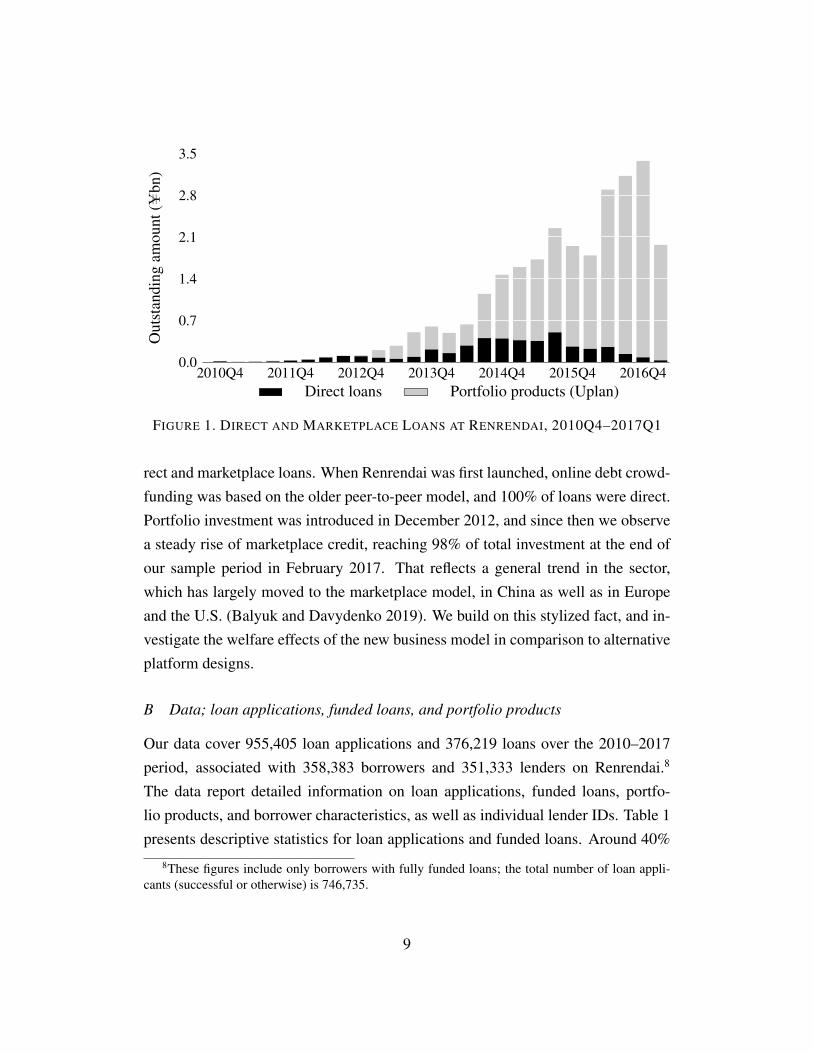
Figure 1 breaks down credit at Renrendai during our sample period between di-

maturity options available to borrowers are 3, 6, 9, 12, 15, 18, 24, and 36 months. Throughoutmost of our sample period, Renrendai sets aside part of its revenues in a reserve pool, intended tocompensate investors who suffered a default on the least risky loan categories. As of 2016Q3, thereserve pool had a size of about U345 million, corresponding to 3.2% of the value of outstandingcredit-certified loans. In late 2016, reserve pools of this sort were abolished by the regulatory reform“Interim Measures for the Administration of the Business Activities of Online Lending InformationIntermediary Institutions,” (网络借贷信息中介机构业务活动管理暂行办法) issued by China’sbanking regulatory commission.

7In addition to Uplan, Renrendai offers another portfolio product called Salary Plan (薪计划),similar to Uplan, but with a fixed 12 months maturity and investment in fixed monthly installmentsrather than a lump sum. Investing in Uplan or Salary Plan involves a 90-day lock-up period. Itis possible for lenders to withdraw their investment before the end of the lock-up period, but thisrequires the payment of a 2% fee; moreover, the lender only receives a payment once Renrendai hasplaced the underlying loans on the secondary market.

8

2010Q4 2011Q4 2012Q4 2013Q4 2014Q4 2015Q4 2016Q40.0

0.7

1.4

2.1

2.8

3.5O

utst

andi

ngam

ount

(Ubn

)

Direct loans Portfolio products (Uplan)

FIGURE 1. DIRECT AND MARKETPLACE LOANS AT RENRENDAI, 2010Q4–2017Q1

rect and marketplace loans. When Renrendai was first launched, online debt crowd-funding was based on the older peer-to-peer model, and 100% of loans were direct.Portfolio investment was introduced in December 2012, and since then we observea steady rise of marketplace credit, reaching 98% of total investment at the end ofour sample period in February 2017. That reflects a general trend in the sector,which has largely moved to the marketplace model, in China as well as in Europeand the U.S. (Balyuk and Davydenko 2019). We build on this stylized fact, and in-vestigate the welfare effects of the new business model in comparison to alternativeplatform designs.

B Data; loan applications, funded loans, and portfolio products

Our data cover 955,405 loan applications and 376,219 loans over the 2010–2017period, associated with 358,383 borrowers and 351,333 lenders on Renrendai.8

The data report detailed information on loan applications, funded loans, portfo-lio products, and borrower characteristics, as well as individual lender IDs. Table 1presents descriptive statistics for loan applications and funded loans. Around 40%

8These figures include only borrowers with fully funded loans; the total number of loan appli-cants (successful or otherwise) is 746,735.

9

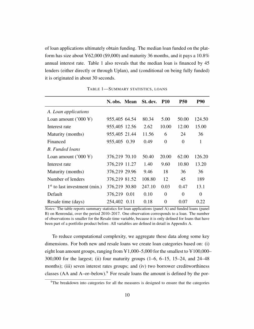
of loan applications ultimately obtain funding. The median loan funded on the plat-form has size about U62,000 ($9,000) and maturity 36 months, and it pays a 10.8%annual interest rate. Table 1 also reveals that the median loan is financed by 45lenders (either directly or through Uplan), and (conditional on being fully funded)it is originated in about 30 seconds.

TABLE 1—SUMMARY STATISTICS, LOANS

N. obs. Mean St. dev. P10 P50 P90

A. Loan applications

Loan amount (’000 U) 955,405 64.54 80.34 5.00 50.00 124.50

Interest rate 955,405 12.56 2.62 10.00 12.00 15.00

Maturity (months) 955,405 21.44 11.56 6 24 36

Financed 955,405 0.39 0.49 0 0 1

B. Funded loans

Loan amount (’000 U) 376,219 70.10 50.40 20.00 62.00 126.20

Interest rate 376,219 11.27 1.40 9.60 10.80 13.20

Maturity (months) 376,219 29.96 9.46 18 36 36

Number of lenders 376,219 81.52 108.80 12 45 189

1st to last investment (min.) 376,219 30.80 247.10 0.03 0.47 13.1

Default 376,219 0.01 0.10 0 0 0

Resale time (days) 254,402 0.11 0.18 0 0.07 0.22Notes: The table reports summary statistics for loan applications (panel A) and funded loans (panelB) on Renrendai, over the period 2010–2017. One observation corresponds to a loan. The numberof observations is smaller for the Resale time variable, because it is only defined for loans that havebeen part of a portfolio product before. All variables are defined in detail in Appendix A.

To reduce computational complexity, we aggregate these data along some keydimensions. For both new and resale loans we create loan categories based on: (i)eight loan amount groups, ranging from U1,000–5,000 for the smallest to U100,000–300,000 for the largest; (ii) four maturity groups (1–6, 6–15, 15–24, and 24–48months); (iii) seven interest rates groups; and (iv) two borrower creditworthinessclasses (AA and A–or–below).9 For resale loans the amount is defined by the por-

9The breakdown into categories for all the measures is designed to ensure that the categories

10

tion of the initial loan that is sold on the secondary market, whereas the maturityis classified as the leftover duration of the loan at the time of resale. As a result,we have 219 loan categories for new and 239 for resale loans (although not allcategories are populated every day in our sample).

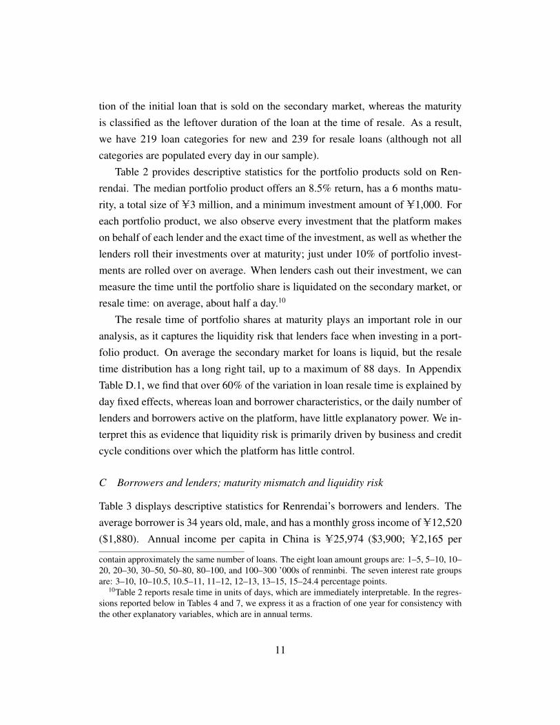
Table 2 provides descriptive statistics for the portfolio products sold on Ren-rendai. The median portfolio product offers an 8.5% return, has a 6 months matu-rity, a total size of U3 million, and a minimum investment amount of U1,000. Foreach portfolio product, we also observe every investment that the platform makeson behalf of each lender and the exact time of the investment, as well as whether thelenders roll their investments over at maturity; just under 10% of portfolio invest-ments are rolled over on average. When lenders cash out their investment, we canmeasure the time until the portfolio share is liquidated on the secondary market, orresale time: on average, about half a day.10

The resale time of portfolio shares at maturity plays an important role in ouranalysis, as it captures the liquidity risk that lenders face when investing in a port-folio product. On average the secondary market for loans is liquid, but the resaletime distribution has a long right tail, up to a maximum of 88 days. In AppendixTable D.1, we find that over 60% of the variation in loan resale time is explained byday fixed effects, whereas loan and borrower characteristics, or the daily number oflenders and borrowers active on the platform, have little explanatory power. We in-terpret this as evidence that liquidity risk is primarily driven by business and creditcycle conditions over which the platform has little control.

C Borrowers and lenders; maturity mismatch and liquidity risk

Table 3 displays descriptive statistics for Renrendai’s borrowers and lenders. Theaverage borrower is 34 years old, male, and has a monthly gross income of U12,520($1,880). Annual income per capita in China is U25,974 ($3,900; U2,165 per

contain approximately the same number of loans. The eight loan amount groups are: 1–5, 5–10, 10–20, 20–30, 30–50, 50–80, 80–100, and 100–300 ’000s of renminbi. The seven interest rate groupsare: 3–10, 10–10.5, 10.5–11, 11–12, 12–13, 13–15, 15–24.4 percentage points.

10Table 2 reports resale time in units of days, which are immediately interpretable. In the regres-sions reported below in Tables 4 and 7, we express it as a fraction of one year for consistency withthe other explanatory variables, which are in annual terms.

11

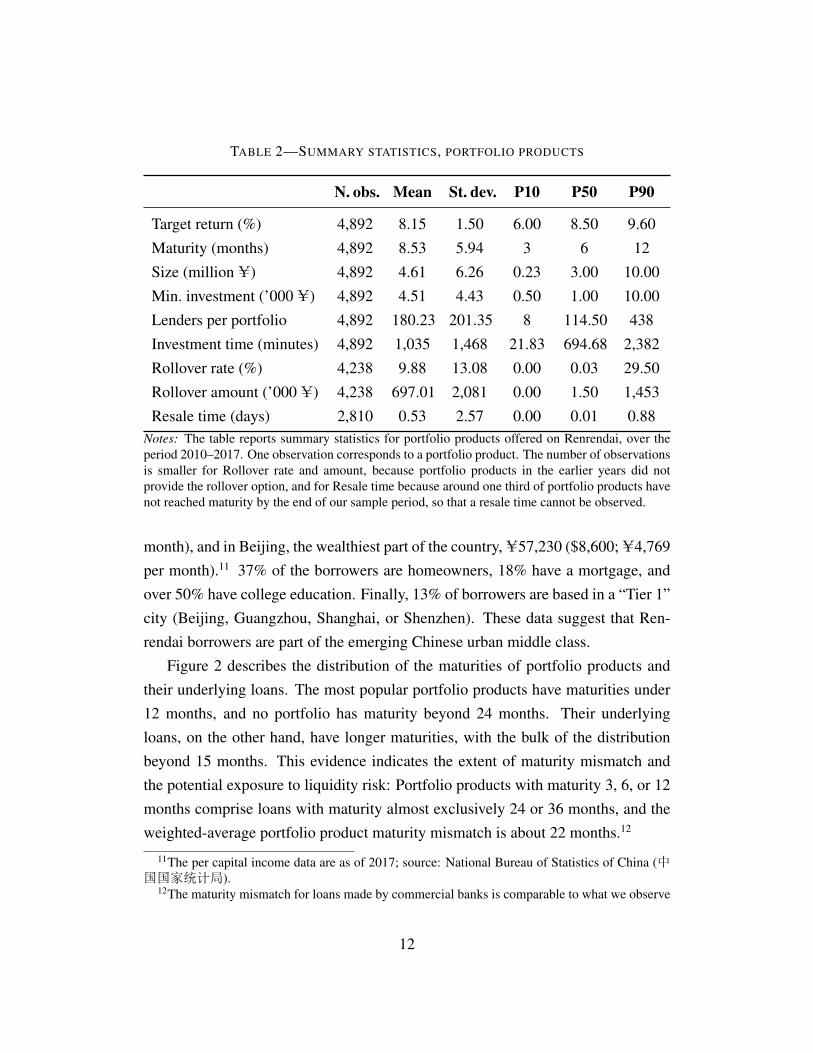
TABLE 2—SUMMARY STATISTICS, PORTFOLIO PRODUCTS

N. obs. Mean St. dev. P10 P50 P90

Target return (%) 4,892 8.15 1.50 6.00 8.50 9.60

Maturity (months) 4,892 8.53 5.94 3 6 12

Size (million U) 4,892 4.61 6.26 0.23 3.00 10.00

Min. investment (’000 U) 4,892 4.51 4.43 0.50 1.00 10.00

Lenders per portfolio 4,892 180.23 201.35 8 114.50 438

Investment time (minutes) 4,892 1,035 1,468 21.83 694.68 2,382

Rollover rate (%) 4,238 9.88 13.08 0.00 0.03 29.50

Rollover amount (’000 U) 4,238 697.01 2,081 0.00 1.50 1,453

Resale time (days) 2,810 0.53 2.57 0.00 0.01 0.88Notes: The table reports summary statistics for portfolio products offered on Renrendai, over theperiod 2010–2017. One observation corresponds to a portfolio product. The number of observationsis smaller for Rollover rate and amount, because portfolio products in the earlier years did notprovide the rollover option, and for Resale time because around one third of portfolio products havenot reached maturity by the end of our sample period, so that a resale time cannot be observed.

month), and in Beijing, the wealthiest part of the country, U57,230 ($8,600; U4,769per month).11 37% of the borrowers are homeowners, 18% have a mortgage, andover 50% have college education. Finally, 13% of borrowers are based in a “Tier 1”city (Beijing, Guangzhou, Shanghai, or Shenzhen). These data suggest that Ren-rendai borrowers are part of the emerging Chinese urban middle class.

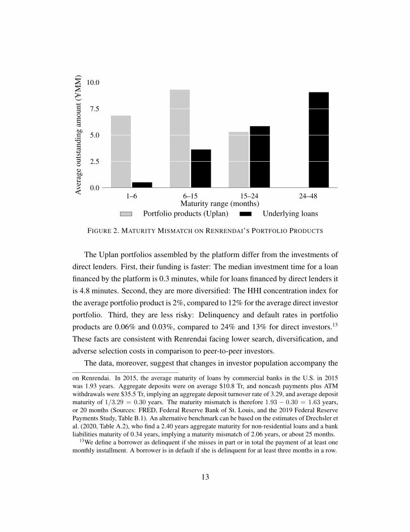
Figure 2 describes the distribution of the maturities of portfolio products andtheir underlying loans. The most popular portfolio products have maturities under12 months, and no portfolio has maturity beyond 24 months. Their underlyingloans, on the other hand, have longer maturities, with the bulk of the distributionbeyond 15 months. This evidence indicates the extent of maturity mismatch andthe potential exposure to liquidity risk: Portfolio products with maturity 3, 6, or 12months comprise loans with maturity almost exclusively 24 or 36 months, and theweighted-average portfolio product maturity mismatch is about 22 months.12

11The per capital income data are as of 2017; source: National Bureau of Statistics of China (中国国家统计局).

12The maturity mismatch for loans made by commercial banks is comparable to what we observe

12

1–6 6–15 15–24 24–480.0

2.5

5.0

7.5

10.0

Maturity range (months)

Ave

rage

outs

tand

ing

amou

nt(U

MM

)

Portfolio products (Uplan) Underlying loans

FIGURE 2. MATURITY MISMATCH ON RENRENDAI’S PORTFOLIO PRODUCTS

The Uplan portfolios assembled by the platform differ from the investments ofdirect lenders. First, their funding is faster: The median investment time for a loanfinanced by the platform is 0.3 minutes, while for loans financed by direct lenders itis 4.8 minutes. Second, they are more diversified: The HHI concentration index forthe average portfolio product is 2%, compared to 12% for the average direct investorportfolio. Third, they are less risky: Delinquency and default rates in portfolioproducts are 0.06% and 0.03%, compared to 24% and 13% for direct investors.13

These facts are consistent with Renrendai facing lower search, diversification, andadverse selection costs in comparison to peer-to-peer investors.

The data, moreover, suggest that changes in investor population accompany the

on Renrendai. In 2015, the average maturity of loans by commercial banks in the U.S. in 2015was 1.93 years. Aggregate deposits were on average $10.8 Tr, and noncash payments plus ATMwithdrawals were $35.5 Tr, implying an aggregate deposit turnover rate of 3.29, and average depositmaturity of 1/3.29 = 0.30 years. The maturity mismatch is therefore 1.93 − 0.30 = 1.63 years,or 20 months (Sources: FRED, Federal Reserve Bank of St. Louis, and the 2019 Federal ReservePayments Study, Table B.1). An alternative benchmark can be based on the estimates of Drechsler etal. (2020, Table A.2), who find a 2.40 years aggregate maturity for non-residential loans and a bankliabilities maturity of 0.34 years, implying a maturity mismatch of 2.06 years, or about 25 months.

13We define a borrower as delinquent if she misses in part or in total the payment of at least onemonthly installment. A borrower is in default if she is delinquent for at least three months in a row.

13

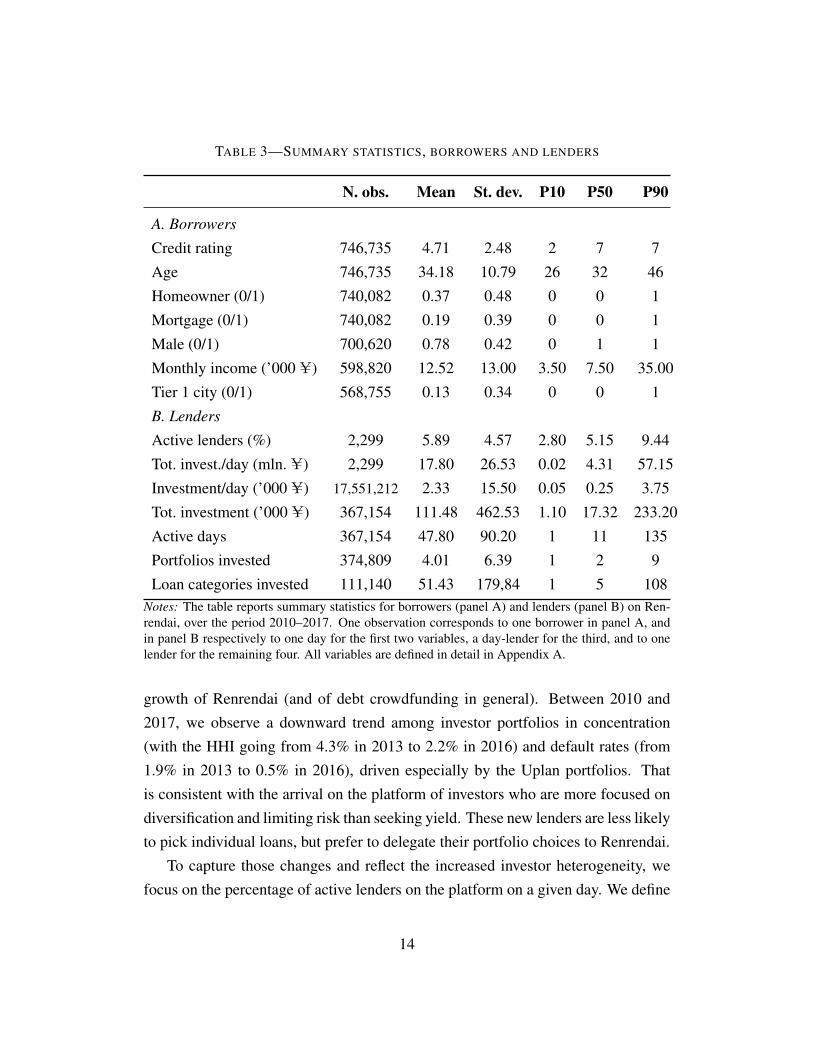
TABLE 3—SUMMARY STATISTICS, BORROWERS AND LENDERS

N. obs. Mean St. dev. P10 P50 P90

A. Borrowers

Credit rating 746,735 4.71 2.48 2 7 7

Age 746,735 34.18 10.79 26 32 46

Homeowner (0/1) 740,082 0.37 0.48 0 0 1

Mortgage (0/1) 740,082 0.19 0.39 0 0 1

Male (0/1) 700,620 0.78 0.42 0 1 1

Monthly income (’000 U) 598,820 12.52 13.00 3.50 7.50 35.00

Tier 1 city (0/1) 568,755 0.13 0.34 0 0 1

B. Lenders

Active lenders (%) 2,299 5.89 4.57 2.80 5.15 9.44

Tot. invest./day (mln. U) 2,299 17.80 26.53 0.02 4.31 57.15

Investment/day (’000 U) 17,551,212 2.33 15.50 0.05 0.25 3.75

Tot. investment (’000 U) 367,154 111.48 462.53 1.10 17.32 233.20

Active days 367,154 47.80 90.20 1 11 135

Portfolios invested 374,809 4.01 6.39 1 2 9

Loan categories invested 111,140 51.43 179,84 1 5 108Notes: The table reports summary statistics for borrowers (panel A) and lenders (panel B) on Ren-rendai, over the period 2010–2017. One observation corresponds to one borrower in panel A, andin panel B respectively to one day for the first two variables, a day-lender for the third, and to onelender for the remaining four. All variables are defined in detail in Appendix A.

growth of Renrendai (and of debt crowdfunding in general). Between 2010 and2017, we observe a downward trend among investor portfolios in concentration(with the HHI going from 4.3% in 2013 to 2.2% in 2016) and default rates (from1.9% in 2013 to 0.5% in 2016), driven especially by the Uplan portfolios. Thatis consistent with the arrival on the platform of investors who are more focused ondiversification and limiting risk than seeking yield. These new lenders are less likelyto pick individual loans, but prefer to delegate their portfolio choices to Renrendai.

To capture those changes and reflect the increased investor heterogeneity, wefocus on the percentage of active lenders on the platform on a given day. We define

14

a lender as active if she is in the top 5% of the distribution of platform use, definedas the number of times she invested up to that date.14 This variable reflects finan-cial constraints: because Renrendai requires a minimum investment amount, morefrequent investments indicate that the lender has greater financial resources, andshould therefore be less liquidity risk–averse. We compute the daily share of activeinvestors as the ratio of active investors to the total number of lenders investing onthe platform on a given day. Descriptives for this variable are reported in Table 3.15

Table 3 also documents that on average each lender invests daily U2,330 and theaggregate daily average investment sums up to U17.8 million. The mean total in-vestment of each lender during the whole sample period is U111,480, spread across48 days of activity, investing on average in 4 portfolios and 51 loan categories.

3 Model

Our model features three players: borrowers, lenders, and a debt crowdfunding plat-form. Borrowers post loan applications and, conditional on the loan being funded,make monthly payments. We treat borrowers as passive agents and focus on thebehavior of the lenders and the platform.16 Lenders can invest in direct loans, orin marketplace loans by acquiring a share of a portfolio product. We model thelenders’ investment decisions using a discrete choice framework, where the lenderschoose among loans and portfolio products based on their characteristics. Condi-tional on investing in a portfolio product, lenders can decide to roll their investmentover at maturity, or cash it out facing the liquidity risk. We use a discrete choiceframework to model the platform’s allocation of portfolio investments across loancategories. The platform maximizes its profits by choosing the target return andthe degree of maturity mismatch for each portfolio product. Appendix Figure D.1

14To control for the time trend in this measure, which might skew the frequency of active lenderstowards the end of the sample period, we define the top 5% based on the platform use distributionwithin each calendar quarter.

15As an alternative, we replace the active lenders share by 1 minus the share of first-time platformusers; the underlying assumption is that first-time users may be more risk averse. We find that it hasa qualitatively similar relation to lender preferences as the active lenders share. These results areomitted for brevity but available upon request.

16The assumption that the borrowers are not strategic is justified by the fact that nearly 80% ofloan applications, and over 95% of funded loans, involve individuals active on Renrendai only once.

15

provides a graphical representation of the model. The next paragraphs describe indetail lender and platform choices.

A Lenders

Every day t a set of lenders i = 1, . . . , It can invest on the platform. Each lendercan choose between investing in direct loans, identified by superscript D, or in aportfolio product, identified by superscript P ; if she invests in a portfolio product,at maturity she also faces the choice between rolling over and cashing out.

In principle, lenders can choose among a large set of direct loans, either newlyposted or trading in the secondary market. Those loans are differentiated by ob-servable characteristics such as yield, maturity, amount, and a number of borrowerattributes. In order to make the lenders’ choice set computationally tractable, as dis-cussed, we group direct loans in discrete categories c = 1, . . . , CD

t , which includeloans that are homogeneous in terms of observable characteristics and are availablefor direct lenders’ investment on day t. A lender chooses to invest in a given loancategory based on the utility she derives from its characteristics. The indirect utilityof lender i investing in loan category c on day t is:

UDict = γrit ln (rct) + γmit ln (mct) + γait ln (act) + γzitzct + ζct︸ ︷︷ ︸

δDict

+εict, (1)

where rct denotes the loan category’s yield, mct its maturity, act its amount, and zctare other characteristics of the loan category observable to the lender (all variablesin Panel A of Table 3, plus time to first investment and time from first to last invest-ment). We group log-yield, log-maturity, log-amount, and zct in a vector xct; ζct arenormally distributed demand shocks at the loan category–day level unobserved bythe econometrician, and εict is a Type 1 Extreme Value shock; letting γit denote thevector of coefficients, we define δDict = γ′itxct + ζct.

To allow for heterogeneity in lender preferences, in equation (1) the coefficientscan vary across lenders i and over time t. That captures the stylized facts describedin Section 2, in particular any change in composition of the lender population to-wards investors with a lower tolerance for liquidity risk. At the same time, it raises

16

the issues of how to measure lender liquidity risk tolerance and how to deal withthe resulting computational complexity. As a proxy for liquidity risk tolerance, asdiscussed we use a measure of the lenders’ activity on the platform. We describeour approach to the computational complexity issue in Section 4 below.

Each lender can also invest in a portfolio product k = 1, . . . , Kt among thoseavailable on a given day t. As remarked, only very rarely we observe lenders fund-ing portfolio products and direct loans simultaneously; we thus treat these two op-tions as mutually exclusive.17 The indirect utility of lender i choosing portfolioproduct k on day t is:

UPikt = αRit ln (Rkt) + αMit ln (Mkt) + αAit ln (Akt) + αZitZkt + ασitσkt + ξkt︸ ︷︷ ︸

δPikt

+ηikt,

(2)where Rkt denotes the target return of portfolio product k, offered on the platformon day t,Mkt its maturity, and Akt its target size; Zkt are other portfolio characte-ristics observable to the lender that we describe in detail in Section 5. σkt denotesthe portfolio product’s liquidity, defined as the time it takes for its underlying loansto be resold on the secondary market at maturity, or resale time. We assume thatlenders have rational expectations of each portfolio’s resale time.18 As in equation(1), the model’s coefficients are allowed to vary across lenders and over time. Alsoas in equation (1), we group log-target return, log-maturity, log-investment amount,and Zkt in a vector of characteristics Xkt; ξkt are normally distributed shocks todemand at the portfolio product–day level unobserved by the econometrician, andηikt is a Type 1 Extreme Value shock; αit denotes the vector of coefficients, andδPikt = α′itXkt + ξkt.19

When the portfolio product reaches maturity, lenders decide whether to roll itover (at the same conditions as they originally invested) or to cash it out. The

17Out of 13,398,102 lender-date observations, we observe lenders holding both a portfolio productand direct loans in 155,604 cases (1.16%).

18We treat σkt as an exogenous portfolio attribute. We discuss this choice in Section 6.C, wherewe argue that our conclusions are not sensitive to it.

19A nested logit approach, with direct and portfolio investment representing the two nests, deliversvery similar results as our current specification (omitted for brevity; available upon request).

17

indirect utility from rolling over is:

URollikt = τRRkt + τMMkt + τAAkt + τZZkt + τσσkt + νikt, (3)

where νjkt is a normally distributed shock.Finally, lenders have the outside option of not investing on the platform. Ideally,

we would like to capture what part of the population of potential lenders (marketsize) does not invest on the platform on a given day. To proxy for that, we assumethat the day with the largest amount invested in a given calendar quarter correspondsto the potential market size in that quarter and define that as Lt; on a given day t, themarket share of the outside option is Lt minus the lenders’ total invested amount.We normalize the indirect utility from choosing the outside option to zero.

The indirect utility from equation (1) determines the probability that lender iinvests in loan category c on day t:

SDict(xct,Xkt | γit, αit) =exp(δDict)

1 +∑

c∈CDt

exp(δDict) +∑

k∈Ktexp(δPikt)

. (4)

Similarly, the indirect utility from equation (2) determines the probability that lenderi invests in portfolio product k at time t, SPikt, whose expression is analogous toequation (4); and the indirect utility from equation (3) determines the probabilitythat she rolls over her investment in portfolio k as opposed to cashing out, SRollikt .

B Platform

The platform’s portfolio choice is treated as an asset demand model based on loancharacteristics, in the spirit of Koijen and Yogo (2019). Each day t, the platformdecides the features of each portfolio product k = 1, . . . , Kt that it offers, andselects the underlying loans. We assume that the loan characteristics xct definedin Section 3.A also identify the loan categories c = 1, . . . , CP

t considered by theplatform when creating portfolio products. We allow the set of loan categoriesavailable to the platform for its portfolios CP

t to be different from those available todirect lendersCD

t , for two reasons. First, the platform only invests in AA borrowers,which mechanically eliminates all categories with A–or–below borrowers. Second,

18

as documented in Section 2.C, the platform is faster than direct lenders at selectingthe loans, and therefore might be able to fund all loans available on a given day forsome of the categories, subtracting those loan categories from the direct lenders’choice set.

The platform receives a total renminbi amount Lt×∑

k∈KtSPkt on day t to invest

in portfolio products. That amount is allocated across portfolios based on theirmarket shares SPkt, which aggregate the individual lender demands SPikt defined inthe previous section. For a given portfolio product k, the total investment amountLtSPkt is entirely allocated across loan categories, with wkct being the weight of loancategory c in portfolio k.

To determine the weights wkct, the platform solves a portfolio allocation prob-lem. Following Koijen and Yogo (2019), we assume that the excess returns on loancategories have a factor structure captured by their characteristics. We can thenmatch observed portfolio weights to recover the platform’s “preferences” for thosecharacteristics, with an approach similar to the discrete-choice framework used forlender demands. The weight wkct of loan category c in portfolio product k offeredon the platform on day t is:

wkct =exp(δkct)∑

g∈CPt

exp(δkgt), (5)

where:δkct = βrktrct + βmktmct + βaact + βzzct + βddct + υkct, (6)

and υkct are normally distributed demand shocks at the portfolio–loan category–day level unobserved by the econometrician. Equation (6) describes the platform’spreferences for loan characteristics associated with a given portfolio product. Forinstance, a higher βr indicates that the platform has a stronger preference for loanswith higher yields, and these loans will constitute a larger share of the portfolio;similarly, a higher βm indicates a stronger preference for loans with longer matu-rity. We let the platform have heterogeneous preferences, varying across portfolioproducts k and days t, for the most relevant loan characteristics: yield and maturity.βrkt captures the platform’s preference in the risk-return tradeoff between earning

19

a greater profit margin rct − Rkt and selecting loans from borrowers with higherwillingness to pay for credit, which might be a signal of low creditworthiness. βmktindicates the platform’s preference for loans with long maturities in portfolio k.A larger βmkt will generate portfolios containing a larger proportion of loans withlonger maturities. As a result, βmkt drives the maturity mismatch in a given portfolioproduct, and thus determines the exposure to liquidity risk.20 For these reasons, wefocus our analysis, and the platform’s optimization problem discussed below, onthese two parameters.

We also assume that the platform has an informational advantage when selectingloans relative to individual investors and is able to predict the average default ratedct. This is a realistic approximation, as the platform has access to the performancerecord of all loans ever granted, whereas individual lenders do not.

In our counterfactual analysis of Section 6, we combine the estimates of thelender demand model with the structure of the platform’s portfolio choice to sim-ulate the welfare effects of alternative scenarios. That requires modeling how theplatform adjusts its target return and maturity preferences to maximize profits. Oneach portfolio product, the platform earns a profit Πkt given by:

Πkt = LtSPkt

∑c∈CP

t

wkct (rct − C1kct)mct −RktMkt − C2kt

, (7)

where LtSPkt is the renminbi amount invested in portfolio product k. The termsin square brackets denote the percentage return that the platform earns on that in-vestment net of its costs. Revenues on portfolio k are measured by

∑cwkctrctmct,

i.e. the platform earns an annualized return rct on loan category c, over a durationof mct years. From that amount, we subtract (i) the target return Rkt paid out tolenders for a duration ofMkt years; (ii) a transaction cost C1kct, capturing the costof locating and monitoring loans in category c; and (iii) an administrative cost C2ktnet of fees, which characterizes portfolio k and does not vary across loan categories.

We model C1kct as βmktmctC1kt, where βmkt denotes the platform’s maturity mis-

20We take the set of available portfolio product maturities as given, as it remains fixed throughoutour data.

20

match parameter from equation (6), and C1kt is a scalar unobserved by the econo-metrician, but which can be recovered using the first-order conditions of the profitfunction as illustrated in Appendix C. The marginal cost C1kct is an increasing func-tion of the loan category maturitymct, capturing the idea that loans with longer ma-turities involve higher screening and monitoring costs (Calomiris and Kahn (1991)).C1kct is also an increasing function of the maturity mismatch parameter βmkt , reflect-ing the fact that the platform will exert more screening and monitoring effort onloans that represent a larger fraction of its portfolio.

In equilibrium, the platform chooses portfolio product characteristics and com-position so as to maximize its overall profit. Operationally, the platform optimallydetermines the target returnRkt and preference for underlying loan maturity βmkt foreach portfolio product.21 The platform solves:

max{Rkt,β

mkt}

Πt =∑k

Πkt. (8)

The solution to problem (8) determines the composition of each portfolio product.

C Equilibrium

Every day t, lenders can invest in CDt loan categories, available both in the primary

and secondary markets for direct loans, and in Kt loan portfolios. The equilibriumis characterized by the conditions defining the lenders’ utility maximization prob-lem, together with the platform’s portfolio allocation and profit maximization prob-lems (borrowers, on the other hand, are treated as passive). Lenders, borrowers andthe platform interact in the primary or the secondary market for loans.

In the primary market, the supply of loans is exogenously given, as borrowerspost loan applications involving a fixed promised interest rate, loan amount, andmaturity. The demand for loans is defined by the direct lenders’ market share equa-

21We solve the platform’s optimization problem as a function of the maturity preference parame-ter βmkt rather than portfolio product maturity as a matter of tractability. There are only a handful ofportfolio maturity options available on the platform (3, 6, 12, 18, and 24 months), whereas focus-ing on βmkt allows us to work with a continuous variable. Moreover, given portfolio maturity, βmktdetermines the extent of maturity mismatch, so that optimizing with respect to βmkt is isomorphic tooptimizing with respect to portfolio maturity.

21

tion (4) and the loan portfolio product weights given by equation (5). The lendersand the platform take loan promised interest rates, amounts, and maturities as given,and as a result a loan application may remain unfunded depending on the lenders’and the platform’s demands.22

In the secondary market, the supply of loans is given by the fraction of loanportfolios that are not rolled over, which in turn is determined by equation (11). Aninstitutional feature of Renrendai is that loans are resold at their face value. Becausethe resale price cannot be adjusted, lenders who do not roll over their portfoliosmay have to hold their loans until a buyer is available; the resale time variable σktcaptures this feature of the secondary market for each portfolio k at its maturity.

The demand for loans is defined, as in the primary market, by the direct lenders’market share equation (4) and the platform’s portfolio weights (5). For each port-folio product k on day t, demand equals supply in equilibrium. The supply ofportfolio products is determined by the platform maximization problem (8), and thedemand by their market shares SPkt.

We define the equilibrium as a set of target returnsRkt and maturity preferencesβmkt such that (i) the platform maximizes the profit function in equation (8); (ii) foreach k and c, the portfolio weight of loan category c in portfolio product k satisfiesequation (5); (iii) for each k, the portfolio product market share satisfies equation(10); (iv) the market share of loans in the secondary market satisfies equation (11);and (v) the market share of direct loans satisfies equation (4).

4 Estimation

We estimate the model outlined in the preceding Sections to recover lender prefe-rences for loans and portfolio products, the determinants of the investment rolloverdecision, and the platform’s preferences for loan characteristics.

Our approach builds on the logit demand for differentiated products model ofBerry (1994), which obtains preference parameter estimates from market shares.We define market shares based on the probability that a given lender choose a givenloan category from equation (4), and analogously for portfolio products. To account

22In the data, about 60% of loan applications are not funded.

22

for lender preference heterogeneity, as discussed we use activity on Renrendai as anindex of lender sophistication and liquidity risk–tolerance. Intuitively, only lenderswith deeper pockets, who have greater capacity to bear liquidity risk, can incur theminimum investment cost frequently. To aggregate this measure across all lendersin equation (4), we focus on the percentage of active lenders (in the top 5% of theactive investing distribution in a given calendar quarter) among all investors whooperate on the platform on a given day t; we denote this measure by Et, and interpretit as the probability that a given lender is active. We can thus write the coefficientsin equations (1) and (4) as γt = γ + ςEt, dropping the subscript j, where γ capturesthe preference of the most inactive lenders and ς measures the deviation from thatbaseline level driven by a higher probability that a given lender is active.

Next, denote by SDct the market share of loan category c on day t and by S0tthe market share of the lenders’ “outside option” of not investing on Renrendai.The natural logarithm of the ratio between SDct and S0t is linear in the preferenceparameters, so that we can estimate:

ln(SDct )−ln(S0t) = γrt ln(rct)+γmt ln(mct)+γat ln(act)+γzt zct+µD+µt+ζct, (9)

where the main explanatory variables are loan return r, maturity m, and amount a,and z collects other loan attributes; µD is an indicator for the direct loans investmentchannel, µt are day fixed effects, and ζct are shocks.

A similar expression obtains for the lenders’ investment in portfolio products:

ln(SPkt)−ln(S0t) = αRt ln(Rkt)+αMt ln(Mkt)+α

At ln(Akt)+αZt Zkt+ασt σkt+µP+µt+ξkt,

(10)where R denotes the portfolio’s target return, M its maturity, A the target sizeof the portfolio, and Z collects other observable attributes of the portfolio. Wealso include liquidity risk σkt (time to resale associated with portfolio k on dayt) in equation (10), as the lender’s payoff at maturity depends on the ability toliquidate the loans in her portfolio on the secondary market; µP is an indicator forthe portfolio investment channel, µt are day fixed effects, and ξkt are shocks. Weestimate equations (9) and (10) as part of one regression model, combining lender

23

choices to invest in direct loans and portfolio products.23

We estimate the determinants of the rollover decision using ordinary least squares.In this case, the dependent variable is the proportion of investment portfolio productk that is rolled over by investors, which we denote with SRollkt :

SRollkt = τRRkt + τMMkt + τAAkt + τZZkt + τσσkt + ψt + νkt, (11)

where ψt denote day fixed effects and νkt are shocks.Finally, we estimate the platform’s demand for loans in a similar fashion as for

equations (9) and (10), but with one important difference. The platform does nothave an outside option, as it needs to invest the whole amount raised from lendersacross loan categories. Hence, to be able to identify the preference parameters weneed to normalize all δkct with respect to one of the alternatives within portfolio kissued on day t. This leads to the following specification:

ln(wkct)− ln(wk0t) = βrkt (rct − r0t) + βmkt (mct −m0t) + βa (act − a0t)

+ βz (zct − z0t) + βd (dct − d0t) + φt + υkct,(12)

where wk0t represents the share invested in the loan category with respect to whichall other categories are normalized, r0t,m0t, a0t, z0t, d0t are its corresponding attri-butes, φt are day fixed effects, and υkct are shocks.

Identification of the lenders’ preference parameters and the platform’s demandfor loans relies on the assumption that the demand shocks ζct, ξkt, and νkt are uncor-related with interest rates, loan amounts, and maturities, conditional on the controlvariables z (Z) and the channel (direct loan/portfolio) and day fixed effects. A vio-lation of this assumption could be driven by omitted variables, if the demand shocksreflect loan or portfolio product qualities that are observed only by the lenders and

23Alternative approaches could be a mixed logit model (Train (2009)) or the random coefficientslogit demand model of Berry et al. (1995). We do not choose the mixed logit approach to containdimensionality and because it would be difficult to identify individual lenders’ choice of an outsideoption. We also do not implement the Berry et al. (1995) approach as it would increase computa-tional complexity, since it does not have a closed form solution for the market shares, and becauseour strategy already captures similar heterogeneity in lender preferences. The Berry et al. (1995) ap-proach would identify the mean and standard deviation of the lender preferences’ distribution, whileour approach delivers estimates of baseline preference parameters and deviations from the baseline.

24

are correlated with interest rates, loan amounts, or maturities. We rely on the institu-tional features of our setting to address this possibility: thanks to the level of detailof our data, we can observe exactly the same information available to the lenders.We can therefore control for every product or loan attribute that investors see whenthey access the platform, thus greatly reducing the scope for omitted variables.

A second potential challenge to identification is simultaneity. This could bean issue if the borrowers are able to observe a loan category–day specific demandshock faced by the lenders (equations (9)–(10)) or the platform (equation (12)) andstrategically adjust their loan applications. Such a degree of sophistication, how-ever, appears unrealistic: around 80% of loan applications are submitted by bor-rowers using the platform for the first time, and Renrendai provides them with noinformation on the lenders’ or the platform’s past choices.

5 Results

In this section we present the estimates of the models from Section 4. Table 4 de-scribes the lenders’ demand for direct loans and portfolio products. Lender utilityis an increasing function of yields for direct loans (column 1) as well as for port-folio products (column 2), even more so when there are more active lenders onRenrendai. Moreover, lenders investing in direct loans have a stronger sensitivityto returns than marketplace investors. As a gauge for that, we look at the estimatesof the elasticity of demand with respect to loan and portfolio returns reported in thefirst two rows of Table 5, which assess the economic significance of the results ofTable 4 considering different percentiles in the distribution of the daily proportionof active lenders. A 10% higher return increases the demand for a given loan cate-gory by 4.6% on average; in comparison, a 10% higher target return raises portfolioproduct demand on average by only 3.2%.

We find that lenders prefer larger loans and portfolios, and such preference doesnot depend on their level of activity on the platform. Direct lenders also preferlonger maturities, whereas portfolio product investors favor shorter portfolio matu-rities, the more so the more active they are on the platform.

Portfolio product investors do not favor a longer resale time, i.e. they are averse

25

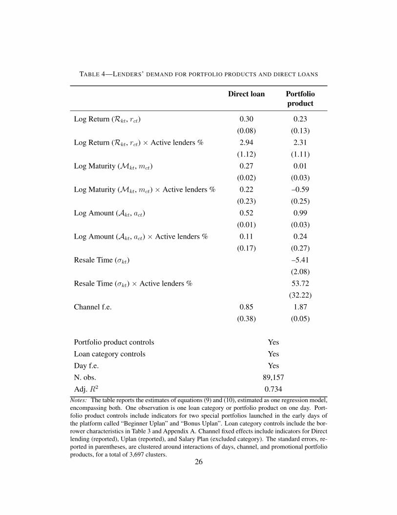
TABLE 4—LENDERS’ DEMAND FOR PORTFOLIO PRODUCTS AND DIRECT LOANS

Direct loan Portfolioproduct

Log Return (Rkt, rct) 0.30 0.23

(0.08) (0.13)

Log Return (Rkt, rct) × Active lenders % 2.94 2.31

(1.12) (1.11)

Log Maturity (Mkt, mct) 0.27 0.01

(0.02) (0.03)

Log Maturity (Mkt, mct) × Active lenders % 0.22 –0.59

(0.23) (0.25)

Log Amount (Akt, act) 0.52 0.99

(0.01) (0.03)

Log Amount (Akt, act) × Active lenders % 0.11 0.24

(0.17) (0.27)

Resale Time (σkt) –5.41

(2.08)

Resale Time (σkt) × Active lenders % 53.72

(32.22)

Channel f.e. 0.85 1.87

(0.38) (0.05)

Portfolio product controls Yes

Loan category controls Yes

Day f.e. Yes

N. obs. 89,157

Adj. R2 0.734Notes: The table reports the estimates of equations (9) and (10), estimated as one regression model,encompassing both. One observation is one loan category or portfolio product on one day. Port-folio product controls include indicators for two special portfolios launched in the early days ofthe platform called “Beginner Uplan” and “Bonus Uplan”. Loan category controls include the bor-rower characteristics in Table 3 and Appendix A. Channel fixed effects include indicators for Directlending (reported), Uplan (reported), and Salary Plan (excluded category). The standard errors, re-ported in parentheses, are clustered around interactions of days, channel, and promotional portfolioproducts, for a total of 3,697 clusters.

26

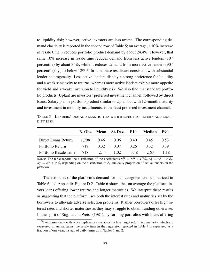
to liquidity risk; however, active investors are less averse. The corresponding de-mand elasticity is reported in the second row of Table 5; on average, a 10% increasein resale time σ reduces portfolio product demand by about 24.4%. However, thatsame 10% increase in resale time reduces demand from less active lenders (10th

percentile) by about 35%, while it reduces demand from more active lenders (90th

percentile) by just below 12%.24 In sum, these results are consistent with substantiallender heterogeneity. Less active lenders display a strong preference for liquidityand a weak sensitivity to returns, whereas more active lenders exhibit more appetitefor yield and a weaker aversion to liquidity risk. We also find that standard portfo-lio products (Uplan) are investors’ preferred investment channel, followed by directloans. Salary plan, a portfolio product similar to Uplan but with 12–month maturityand investment in monthly installments, is the least preferred investment channel.

TABLE 5—LENDERS’ DEMAND ELASTICITIES WITH RESPECT TO RETURN AND LIQUI-DITY RISK

N. Obs. Mean St. Dev. P10 Median P90

Direct Loans Return 1,798 0.46 0.06 0.40 0.45 0.53

Portfolio Return 718 0.32 0.07 0.26 0.32 0.39

Portfolio Resale Time 718 –2.44 1.02 –3.48 –2.63 –1.18Notes: The table reports the distribution of the coefficients γRt = γR + ςREt, γrt = γr + ςrEt,ασt = ασ + ςσEt depending on the distribution of Et, the daily proportion of active lenders on theplatform.

The estimates of the platform’s demand for loan categories are summarized inTable 6 and Appendix Figure D.2. Table 6 shows that on average the platform fa-vors loans offering lower returns and longer maturities. We interpret these resultsas suggesting that the platform uses both the interest rates and maturities set by theborrowers to alleviate adverse selection problems. Riskier borrowers offer high in-terest rates and shorter maturities as they may struggle to obtain funding otherwise.In the spirit of Stiglitz and Weiss (1981), by forming portfolios with loans offering

24For consistency with other explanatory variables such as target return and maturity, which areexpressed in annual terms, the resale time in the regression reported in Table 4 is expressed as afraction of one year, instead of daily terms as in Tables 1 and 2.

27

lower interest rates and longer maturities, the platform obtains lower returns on theaverage loan but extends credit to a pool of safer borrowers.25 Interestingly, thatcontrasts with the behavior of direct lenders, who, as we discussed, favor higherreturns. These findings are consistent with the descriptive evidence of Section 2.B,showing that portfolio products are more diversified and have lower default ratesthan direct lender portfolios.26 This interpretation is corroborated by the results inTable 6, which show that the platform avoids loan categories with higher defaultrates.27 We also find that, ceteris paribus, the platform prefers primary market loansto loans available on the secondary market. This makes intuitive sense because pri-mary market loans are more profitable to the platform, as the borrowers pay a feewhen they obtain a loan, but not when the loan is resold.

Finally, Table 7 describes the lenders’ rollover decision. Rollover probabilityfor a portfolio product is increasing in its return and size, and decreasing in ma-turity. The estimates of Table 7 suggest that portfolio product characteristics havevery little impact on the fraction of the portfolio that is rolled over. The coefficientson target return and resale time are insignificantly different from zero at conven-tional levels, and the coefficients on maturity and portfolio size, although signifi-cantly different from zero, imply small economic effects.28 This is in line with thedescriptive evidence of Section 2, suggesting that the platform has little ability to

25Hertzberg, Liberman and Paravisini (2018), using data from the U.S. marketplace lending plat-form Lending Club, find that riskier borrowers self-select into longer maturities. That is due tothe fact that Lending Club uses maturities to screen borrowers, by assigning higher interest rates tolonger-maturity loans—in their setting, riskier borrowers are willing to pay a higher interest rate asa form of insurance against having to roll over their loan at unfavorable conditions. On Renrendai,prospective borrowers have much more flexibility when they apply for a loan, and in particular theinterest rate they can offer to pay is only required to be within a broad band, so that maturity is nota screening tool.

26Our interpretation of the results is that risky borrowers do not learn that by posting lower interestrates they may increase their chances of being funded. This argument is backed by our institutionalsetting: Over 95% of funded loans are granted to borrowers using the platform for the first time.

27Note that we use the realized default rates in each loan category up to time t. In other words,we assume that the platform can predict the average defaults in each category using the informationit holds about the past records on loan performance.

28In the estimates of Table 7, maturity is expressed in years. The coefficient estimate of −0.01implies that a one-year shorter maturity is associated with a 1 percentage point larger share of theportfolio that is rolled over. Given that the longest portfolio product maturity in our data is threeyears, the effect is very modest. Similarly, a one–standard deviation (U6.26) increase in portfoliosize is associated with a 6 percentage points higher rollover rate.

28

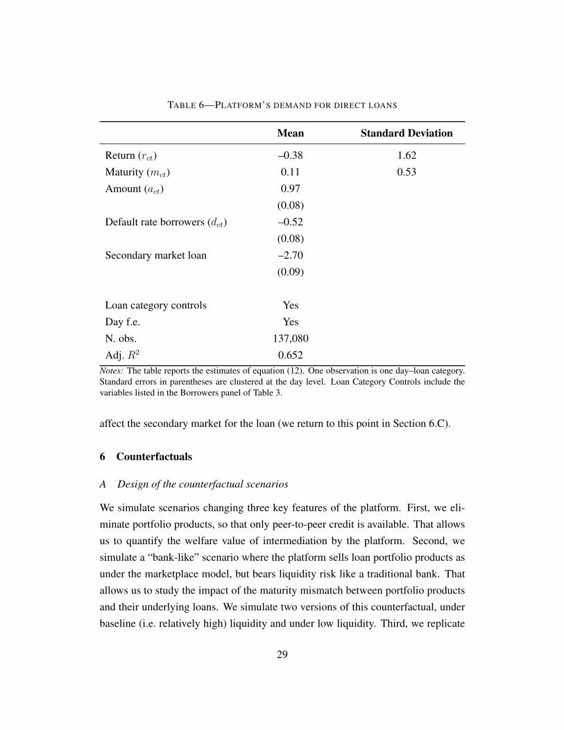
TABLE 6—PLATFORM’S DEMAND FOR DIRECT LOANS

Mean Standard Deviation

Return (rct) –0.38 1.62

Maturity (mct) 0.11 0.53

Amount (act) 0.97

(0.08)

Default rate borrowers (dct) –0.52

(0.08)

Secondary market loan –2.70

(0.09)

Loan category controls Yes

Day f.e. Yes

N. obs. 137,080

Adj. R2 0.652Notes: The table reports the estimates of equation (12). One observation is one day–loan category.Standard errors in parentheses are clustered at the day level. Loan Category Controls include thevariables listed in the Borrowers panel of Table 3.

affect the secondary market for the loan (we return to this point in Section 6.C).

6 Counterfactuals

A Design of the counterfactual scenarios

We simulate scenarios changing three key features of the platform. First, we eli-minate portfolio products, so that only peer-to-peer credit is available. That allowsus to quantify the welfare value of intermediation by the platform. Second, wesimulate a “bank-like” scenario where the platform sells loan portfolio products asunder the marketplace model, but bears liquidity risk like a traditional bank. Thatallows us to study the impact of the maturity mismatch between portfolio productsand their underlying loans. We simulate two versions of this counterfactual, underbaseline (i.e. relatively high) liquidity and under low liquidity. Third, we replicate

29

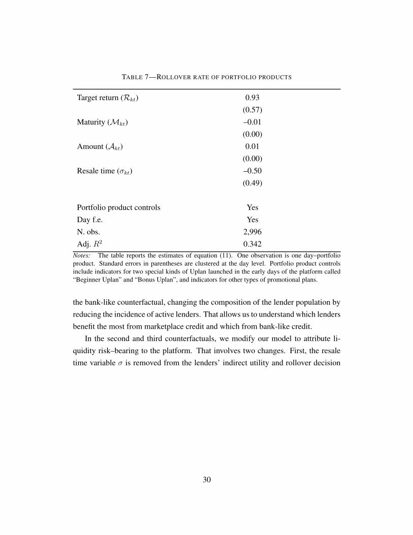
TABLE 7—ROLLOVER RATE OF PORTFOLIO PRODUCTS

Target return (Rkt) 0.93

(0.57)

Maturity (Mkt) –0.01

(0.00)

Amount (Akt) 0.01

(0.00)

Resale time (σkt) –0.50

(0.49)

Portfolio product controls Yes

Day f.e. Yes

N. obs. 2,996

Adj. R2 0.342Notes: The table reports the estimates of equation (11). One observation is one day–portfolioproduct. Standard errors in parentheses are clustered at the day level. Portfolio product controlsinclude indicators for two special kinds of Uplan launched in the early days of the platform called“Beginner Uplan” and “Bonus Uplan”, and indicators for other types of promotional plans.

the bank-like counterfactual, changing the composition of the lender population byreducing the incidence of active lenders. That allows us to understand which lendersbenefit the most from marketplace credit and which from bank-like credit.

In the second and third counterfactuals, we modify our model to attribute li-quidity risk–bearing to the platform. That involves two changes. First, the resaletime variable σ is removed from the lenders’ indirect utility and rollover decision

30

equations. Second, the profit on a given portfolio product k is now written as:

Πkt = SPktLt

{ ∑c∈m≤M

wkct (rct − C1kct)mct︸ ︷︷ ︸No liquidity

risk

+∑

c∈m>M

wkct (rct − C1kct)[mct −

(1− SRollkt

) mct

Mkt

σct

]︸ ︷︷ ︸

Liquidityrisk

−RktMkt − C2kt

}.

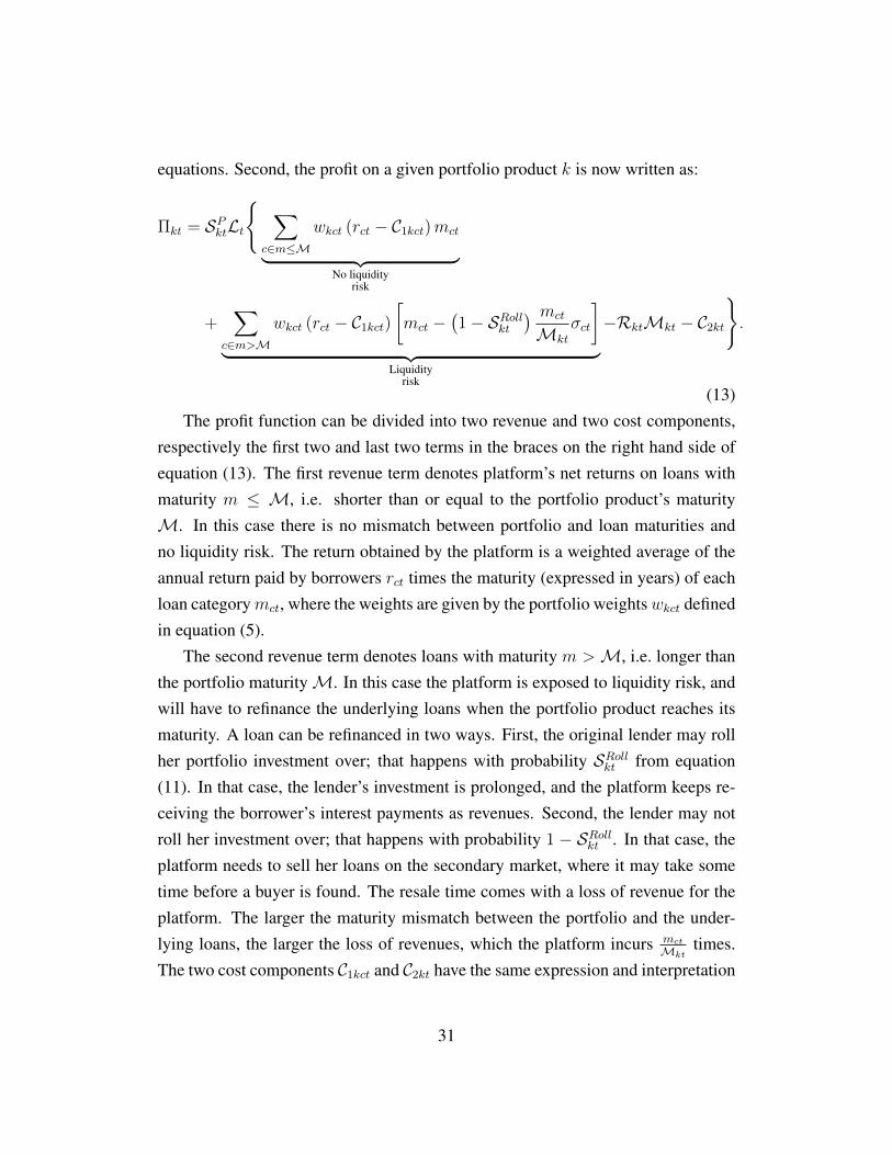
(13)The profit function can be divided into two revenue and two cost components,

respectively the first two and last two terms in the braces on the right hand side ofequation (13). The first revenue term denotes platform’s net returns on loans withmaturity m ≤ M, i.e. shorter than or equal to the portfolio product’s maturityM. In this case there is no mismatch between portfolio and loan maturities andno liquidity risk. The return obtained by the platform is a weighted average of theannual return paid by borrowers rct times the maturity (expressed in years) of eachloan categorymct, where the weights are given by the portfolio weightswkct definedin equation (5).

The second revenue term denotes loans with maturity m >M, i.e. longer thanthe portfolio maturityM. In this case the platform is exposed to liquidity risk, andwill have to refinance the underlying loans when the portfolio product reaches itsmaturity. A loan can be refinanced in two ways. First, the original lender may rollher portfolio investment over; that happens with probability SRollkt from equation(11). In that case, the lender’s investment is prolonged, and the platform keeps re-ceiving the borrower’s interest payments as revenues. Second, the lender may notroll her investment over; that happens with probability 1 − SRollkt . In that case, theplatform needs to sell her loans on the secondary market, where it may take sometime before a buyer is found. The resale time comes with a loss of revenue for theplatform. The larger the maturity mismatch between the portfolio and the under-lying loans, the larger the loss of revenues, which the platform incurs mct

Mkttimes.

The two cost components C1kct and C2kt have the same expression and interpretation

31

as under the marketplace model.The profit function in equation (13) illustrates the tradeoffs faced by the plat-

form when setting portfolio target returns and maturity mismatch under the bank-like scenario. The platform’s profits are decreasing in the return offered to thelenders; but at the same time, the portfolio product market share SPkt is increasingin the target return, and so is the rollover probability SRollkt , raising the platform’sprofits. Moreover, loans with longer maturities provide higher returns; but at thesame time they expose the platform to more liquidity risk.29

B Results

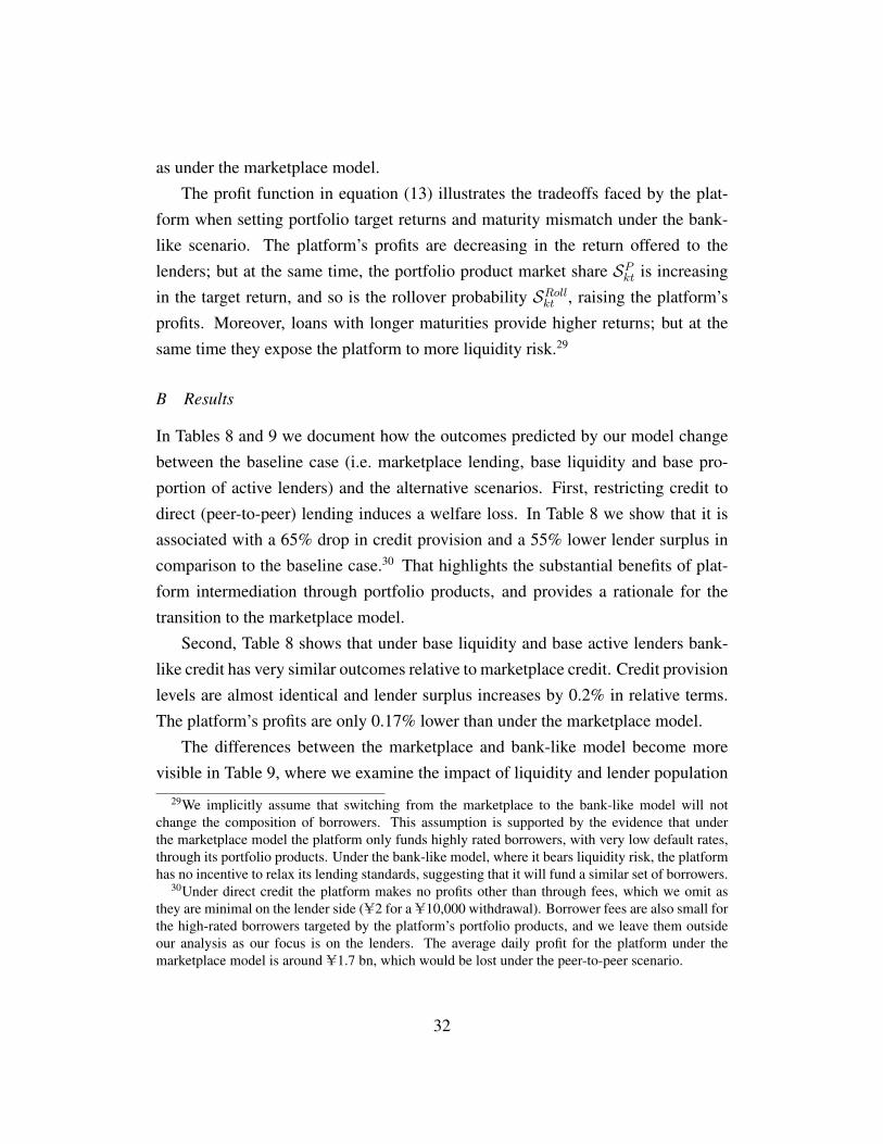
In Tables 8 and 9 we document how the outcomes predicted by our model changebetween the baseline case (i.e. marketplace lending, base liquidity and base pro-portion of active lenders) and the alternative scenarios. First, restricting credit todirect (peer-to-peer) lending induces a welfare loss. In Table 8 we show that it isassociated with a 65% drop in credit provision and a 55% lower lender surplus incomparison to the baseline case.30 That highlights the substantial benefits of plat-form intermediation through portfolio products, and provides a rationale for thetransition to the marketplace model.

Second, Table 8 shows that under base liquidity and base active lenders bank-like credit has very similar outcomes relative to marketplace credit. Credit provisionlevels are almost identical and lender surplus increases by 0.2% in relative terms.The platform’s profits are only 0.17% lower than under the marketplace model.

The differences between the marketplace and bank-like model become morevisible in Table 9, where we examine the impact of liquidity and lender population

29We implicitly assume that switching from the marketplace to the bank-like model will notchange the composition of borrowers. This assumption is supported by the evidence that underthe marketplace model the platform only funds highly rated borrowers, with very low default rates,through its portfolio products. Under the bank-like model, where it bears liquidity risk, the platformhas no incentive to relax its lending standards, suggesting that it will fund a similar set of borrowers.

30Under direct credit the platform makes no profits other than through fees, which we omit asthey are minimal on the lender side (U2 for a U10,000 withdrawal). Borrower fees are also small forthe high-rated borrowers targeted by the platform’s portfolio products, and we leave them outsideour analysis as our focus is on the lenders. The average daily profit for the platform under themarketplace model is around U1.7 bn, which would be lost under the peer-to-peer scenario.

32

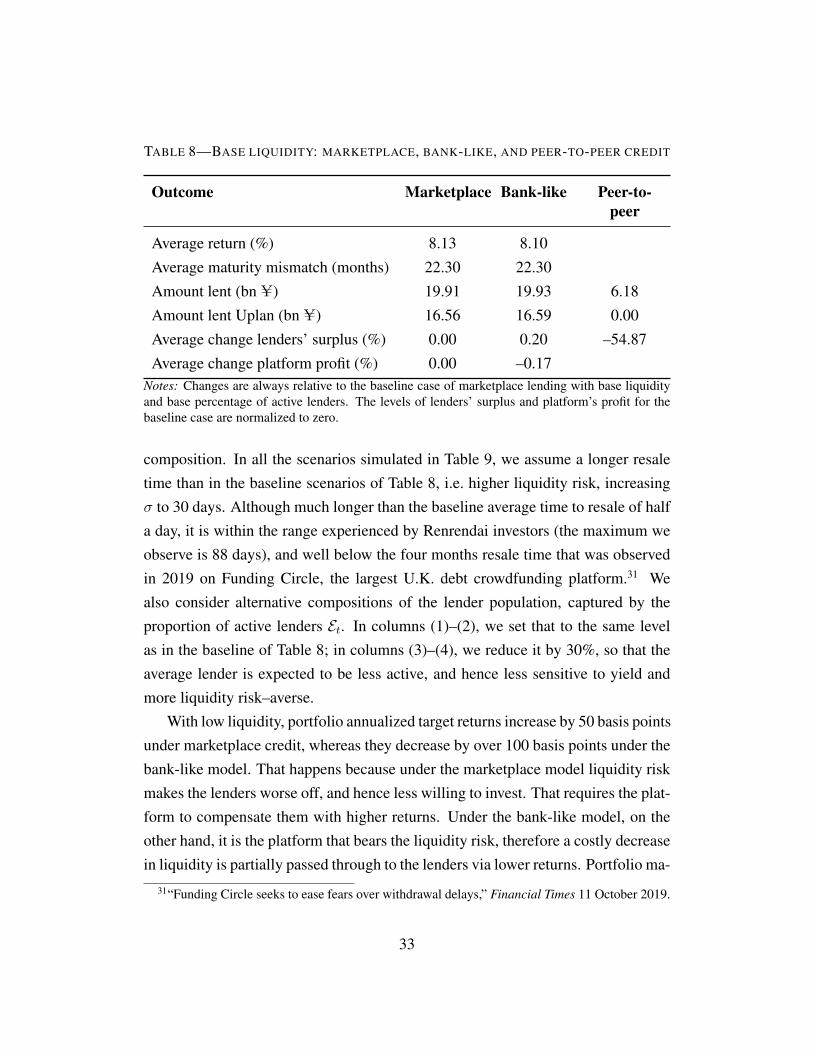
TABLE 8—BASE LIQUIDITY: MARKETPLACE, BANK-LIKE, AND PEER-TO-PEER CREDIT

Outcome Marketplace Bank-like Peer-to-peer

Average return (%) 8.13 8.10

Average maturity mismatch (months) 22.30 22.30

Amount lent (bn U) 19.91 19.93 6.18

Amount lent Uplan (bn U) 16.56 16.59 0.00

Average change lenders’ surplus (%) 0.00 0.20 –54.87

Average change platform profit (%) 0.00 –0.17Notes: Changes are always relative to the baseline case of marketplace lending with base liquidityand base percentage of active lenders. The levels of lenders’ surplus and platform’s profit for thebaseline case are normalized to zero.

composition. In all the scenarios simulated in Table 9, we assume a longer resaletime than in the baseline scenarios of Table 8, i.e. higher liquidity risk, increasingσ to 30 days. Although much longer than the baseline average time to resale of halfa day, it is within the range experienced by Renrendai investors (the maximum weobserve is 88 days), and well below the four months resale time that was observedin 2019 on Funding Circle, the largest U.K. debt crowdfunding platform.31 Wealso consider alternative compositions of the lender population, captured by theproportion of active lenders Et. In columns (1)–(2), we set that to the same levelas in the baseline of Table 8; in columns (3)–(4), we reduce it by 30%, so that theaverage lender is expected to be less active, and hence less sensitive to yield andmore liquidity risk–averse.

With low liquidity, portfolio annualized target returns increase by 50 basis pointsunder marketplace credit, whereas they decrease by over 100 basis points under thebank-like model. That happens because under the marketplace model liquidity riskmakes the lenders worse off, and hence less willing to invest. That requires the plat-form to compensate them with higher returns. Under the bank-like model, on theother hand, it is the platform that bears the liquidity risk, therefore a costly decreasein liquidity is partially passed through to the lenders via lower returns. Portfolio ma-

31“Funding Circle seeks to ease fears over withdrawal delays,” Financial Times 11 October 2019.

33

turity mismatch, on the other hand, adjusts very little. That makes intuitive sense,given that the distribution of maturities sought by the borrowers is stable acrossdifferent scenarios, and so is the set of portfolio maturity categories offered by theplatform. The behavior of target returns and maturity mismatch can also be seen inFigure 3, for the case of base active lenders.

The marketplace and bank-like models have different welfare effects for theplatform, lenders, and borrowers. In columns 1–2 of Table 9, assuming the samelevel of lender liquidity risk–aversion as in our baseline, marketplace credit exhibitsa larger reduction in credit provision and lenders’ surplus, but a smaller reductionin profits, relative to the bank-like model. In other words: with less liquidity inthe secondary market, the platform prefers operating under the marketplace model,whereas borrowers and lenders would be better off under the bank-like model.

The welfare comparison changes, however, in columns 3–4 where we reduce theproportion of active lenders, skewing the lender population towards having greaterliquidity risk aversion and a lower sensitivity to yields on average (illustrated bythe low active lenders case in Figures 3 and 4). Under that scenario, the bank-likemodel is welfare-improving across all three dimensions: we observe greater creditprovision, lender surplus, and platform profits than under the marketplace model.This happens because less active lenders increase the amount they invest in the port-folio products as the platform insures them against liquidity risk. Higher lendingvolumes more than compensate the cost of bearing the liquidity risk, thus increasingthe platform’s profits. This result provides a rationale for the existence of market-place credit alongside traditional banks. When liquidity risk is limited and onlinecredit platforms attract more sophisticated, less liquidity risk–averse investors, themarketplace model can be optimal. In contrast, when liquidity risk is higher and/orwhen investors are more liquidity risk–averse, traditional intermediation dominates(corresponding to the bank-like model in our counterfactual). These observationssuggest that, as debt crowdfunding becomes a more widespread investment channeland reaches a broader population of potential lenders, platforms may start offeringproducts closer to the bank-like model.32

32Two of the largest European players, Zopa and Bondora, are examples of online platformsevolving towards this direction. Zopa recently acquired a banking license in the U.K. and is plan-

34

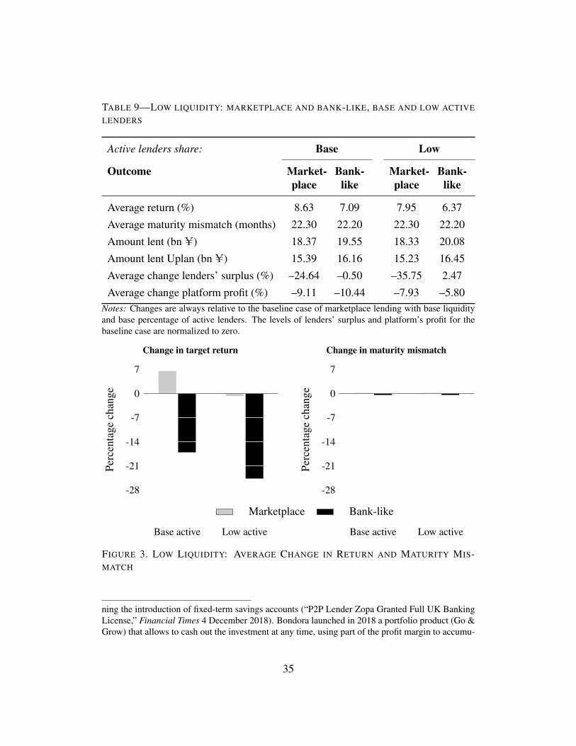
TABLE 9—LOW LIQUIDITY: MARKETPLACE AND BANK-LIKE, BASE AND LOW ACTIVE

LENDERS

Active lenders share: Base Low

Outcome Market-place

Bank-like

Market-place

Bank-like

Average return (%) 8.63 7.09 7.95 6.37

Average maturity mismatch (months) 22.30 22.20 22.30 22.20

Amount lent (bn U) 18.37 19.55 18.33 20.08

Amount lent Uplan (bn U) 15.39 16.16 15.23 16.45

Average change lenders’ surplus (%) –24.64 –0.50 –35.75 2.47

Average change platform profit (%) –9.11 –10.44 –7.93 –5.80Notes: Changes are always relative to the baseline case of marketplace lending with base liquidityand base percentage of active lenders. The levels of lenders’ surplus and platform’s profit for thebaseline case are normalized to zero.

Change in target return

Base active Low active

-28

-21

-14

-7

0

7

Perc

enta

gech

ange

Marketplace

Change in maturity mismatch

Base active Low active

-28

-21

-14

-7

0

7

Perc

enta

gech

ange

Bank-like

FIGURE 3. LOW LIQUIDITY: AVERAGE CHANGE IN RETURN AND MATURITY MIS-MATCH

ning the introduction of fixed-term savings accounts (“P2P Lender Zopa Granted Full UK BankingLicense,” Financial Times 4 December 2018). Bondora launched in 2018 a portfolio product (Go &Grow) that allows to cash out the investment at any time, using part of the profit margin to accumu-

35

Cha

nge

inle

nder

surp

lus

Bas

eac

tive

Low

activ

e

-28

-21

-14-70

Percentagechange

Cha

nge

inpl

atfo

rmpr

ofits

Bas

eac

tive

Low

activ

e

-28

-21

-14-70

Percentagechange

Cha

nge

inam

ount

lent

Bas

eac

tive

Low

activ

e

-28

-21

-14-70

Percentagechange

Mar

ketp

lace

Ban

k-lik

e

FIG

UR

E4.

LO

WL

IQU

IDIT

Y:

AV

ER

AG

EC

HA

NG

EIN

LE

ND

ER

SU

RP

LU

S,P

LA

TF

OR

MP

RO

FIT,

AN

DA

MO

UN

TL

EN

T

36

C Should resale time be endogenous?

We do not explicitly model the mechanism that determines resale time σkt, nor dowe allow the platform to optimize over it. Three reasons motivate this choice. First,it is not obvious that the platform can affect resale time to begin with. The evidencediscussed in Section 2 indicates that resale time is largely driven by business andcredit cycle fluctuations, over which the platform has little control.33

Second, endogenizing resale time increases the model’s computational com-plexity. It requires that lenders and the platform choose not only in what loans toinvest, but also at what time to invest within a given day, increasing the dimen-sionality. In addition, portfolio resale time depends on factors that are realized atportfolio maturity, such as future demand shocks, target returns, and maturity pre-ferences, which in turn depend on the resale time of future loans and portfolios.Treating resale time as endogenous thus gives the model a recursive nature, at theexpense of tractability.

Third, endogenizing resale time is unlikely to deliver additional economic in-sights. Table 9 and Figure 4 indicate that, as the lender population becomes moreliquidity risk–averse, the platform prefers to operate under the bank-like model,rather than the marketplace model. Suppose that the platform could optimally setσ, and consider whether that conclusion changes. Under the bank-like model, anincrease in lender liquidity risk–aversion does not affect the platform’s choice of σ,because the lenders do not bear the cost of a longer resale time. Under the mar-ketplace model an increase in lender liquidity risk–aversion creates an incentive forthe platform to reduce σ, as it affects lender demands and, through them, platformprofits.34 Therefore, as long as reducing resale time imposes an additional cost onthe platform (e.g., in terms of searching and organizing loans as represented by theterm C1kct in equation (7)), a sufficiently high level of lender liquidity risk–aversionwill induce the platform to prefer the bank-like model, thus confirming the findings

late a liquidity reserve for this purpose.33This is in line with the findings of Ba, Bai and Li (2019) and Li, Zhang and Zhao (2019).34Rather than reducing σ, in the marketplace model the platform could offer lenders a higher

target return R; however, that will also lower the platform’s profits. Moreover, as shown in Table5, lender preferences are more sensitive to resale time than to target returns, potentially making anadjustment based solely on target returns very costly.

37

of our counterfactuals.

7 Conclusion

We develop an equilibrium model of online debt crowdfunding to quantify the wel-fare effects of the marketplace credit business model, where the crowdfunding plat-form sells loan portfolio products to lenders. That brings platforms closer to banks,because portfolio products are shorter-term liabilities invested in longer-term loans;but unlike bank depositors, marketplace lenders bear liquidity risk when they wantto cash our their investment.

We estimate our model using the universe of loans and loan applications onRenrendai, a leading Chinese marketplace credit platform. Our approach recov-ers lender preferences from observed investment choices, and allows us to simu-late counterfactuals to contrast marketplace credit to the older peer-to-peer lendingparadigm and to a bank-like model where the platform bears liquidity risk.

We show a transition away from peer-to-peer lending and towards marketplacecredit, and we document and quantify the exposure to liquidity risk that it creates.Moreover, we provide evidence of lender heterogeneity: less active investors onthe platform are less focused on yields and more averse to liquidity risk. Finally,our counterfactual analysis points to two main results. First, moving from the peer-to-peer to the marketplace model raises lender surplus, platform profits, and creditprovision, suggesting a Pareto improvement. Second, the marketplace and bank-like models have similar welfare performance when liquidity is high and lenderliquidity–risk aversion low, but the bank-like model is welfare-increasing when li-quidity is low and lender liquidity–risk aversion high.

Our results highlight the importance of liquidity risk on debt crowdfunding plat-forms, and can contribute to the ongoing regulatory debate, especially relevant asonline credit platforms apply for banking licenses. Our work can also serve as atractable starting point to explore further questions. We see as interesting extensionsto our framework a model that endogenizes credit demand, as well as quantifyingthe differences in costs between marketplace and traditional lending, due to eithertechnological or regulatory differences.

38

References

Ba, S. H., H. Bai, and Y. Li, “P2P wang dài píngtái jiduì fengxian: Jiyú zhàiquánzhuanràng de shìjiao: Cáijing wèntí yànjiu. [P2P online lending platform runrisk: Based on the perspective of debt transfer],” Research on Financial andEconomic Issues, 2019, 1, 52–58.

Balyuk, T. and S. Davydenko, “Reintermediation in FinTech: Evidence fromOnline Lending,” 2019. Working Paper, Emory University Goizueta BusinessSchool.

Berry, S., “Estimating Discrete-Choice Models of Product Differentiation,” RANDJournal of Economics, 1994, 25 (2), 242–262., J. Levinsohn, and A. Pakes, “Automobile Prices in Market Equilibrium,”Econometrica, 1995, 63 (4), 841–890.

BIS, “FinTech Credit: Market Structure, Business Models and Financial StabilityImplications,” Report by Bank for International Settlements Committee on theGlobal Financial System (CGFS) and the Financial Stability Board (FSB), 2017.

Buchak, G., G. Matvos, T. Piskorski, and A. Seru, “Fintech, Regulatory Arbi-trage, and the Rise of Shadow Banks,” Journal of Financial Economics, 2018,130 (3), 453–483.

Calomiris, C. W. and C. M. Kahn, “The Role of Demandable Debt in Structur-ing Optimal Banking Arrangements,” American Economic Review, 1991, 81 (3),497–513.

Crawford, G. S., N. Pavanini, and F. Schivardi, “Asymmetric Information andImperfect Competition in Lending Markets,” American Economic Review, 2018,108 (7), 1659–1701.

de Roure, C., L. Pelizzon, and A. Thakor, “P2P Lenders versus Banks: CreamSkimming or Bottom Fishing?,” 2019. SAFE working paper 206.

Diamond, D. W., “Financial Intermediation and Delegated Monitoring,” Review ofEconomic Studies, 1984, 51 (3), 393–414.and P. H. Dybvig, “Bank Runs, Deposit Insurance, and Liquidity,” Journal of

Political Economy, 1983, 91 (3), 401–419.Dinerstein, M., L. Einav, J. Levin, and N. Sundaresan, “Consumer Price Search

and Platform Design in Internet Commerce,” American Economic Review, 2018,108 (7), 1820–1859.

Drechsler, I., A. Savov, and P. Schnabl, “Banking on deposits: Maturity transfor-mation without interest rate risk,” 2020. Working paper, NYU Stern School ofBusiness.

Egan, M., A. Hortaçsu, and G. Matvos, “Deposit Competition and FinancialFragility: Evidence from the U.S. Banking Sector,” American Economic Review,2017, 107 (1), 169–216.

39

Einav, L., C. Farronato, and J. Levin, “Peer-to-Peer Markets,” Annual Review ofEconomics, 2016, 8, 615–635., , , and N. Sundaresan, “Auctions versus Posted Prices in Online Markets,”Journal of Political Economy, 2018, 126 (1), 178–215.

Farronato, C. and A. Fradkin, “The Welfare Effect of Peer Entry in the Accom-modation Market: The Case of Airbnb,” 2018. NBER Working Paper No. 24361.

Franks, J. R., N. Serrano-Velarde, and O. Sussman, “Marketplace Lending, In-formation Aggregation, and Liquidity,” 2020. Review of Financial Studies, forth-coming.

Fréchette, G. R., A. Lizzeri, and T. Salz, “Frictions in a Competitive, RegulatedMarket Evidence from Taxis,” 2019. American Economic Review, forthcoming.

Goldstein, I. and A. Pauzner, “Demand-Deposit Contracts and the Probability ofBank Runs,” Journal of Finance, 2005, 60 (3), 1293–1327.

Hertzberg, A., A. Liberman, and D. Paravisini, “Screening on Loan Terms: Ev-idence from Maturity Choice in Consumer Credit,” Review of Financial Studies,2018, 31 (9), 3532–3567.

Kawai, K., K. Onishi, and K. Uetake, “Signaling in Online Credit Markets,” 2016.Working Paper, New York University.

Koijen, R. S. J. and M. Yogo, “A Demand System Approach to Asset Pricing,”Journal of Political Economy, 2019, 127 (4), 1475–1515.

Li, J., S. Zhang, and D. Zhao, “P2P wangluò jièdài, liúdòng xìng fengxian yuhóngguan shenshèn zhèngcè. Dangdài jingjì kexué [P2P Online Lending, Liqui-dity Risk and Macro-prudential Policies],” Modern Economic Science, 2019, 5,38–51.

Ma, Y., K. Xiao, and Y. Zeng, “Bank Debt versus Mutual Fund Equity in LiquidityProvision,” 2020. Working Paper, Columbia University.

Rau, P. R., “Law, Trust, and the Development of Crowdfunding,” 2019. WorkingPaper, University of Cambridge Judge Business School.

Stiglitz, J. and A. Weiss, “Credit Rationing in Markets with Imperfect Informa-tion,” American Economic Review, 1981, 71 (3), 393–410.

Tang, H., “The Value of Privacy: Evidence from Online Borrowers,” 2020. Work-ing Paper, London School of Economics and Political Science.

Train, K. E., Discrete Choice Methods with Simulation, Cambridge UniversityPress, 2009.

Vallée, B. and Y. Zeng, “Marketplace Lending: A New Banking Paradigm?,” Re-view of Financial Studies, 2019, 32 (5), 1939–1982.

Xin, Y., “Asymmetric Information, Reputation, and Welfare in Online Credit Mar-kets,” 2018. Working Paper, Johns Hopkins University.

40

For Online Publication—Appendix

A Variable definitions

LOAN APPLICATIONS

Loan Amount (’000 U) Amount of the loan in renminbi

Interest Rate (%) Interest rate offered by the borrower in his/her loan application

Maturity (months) Maturity of the loan as expressed in the in the application (inmonths)

Financed (0/1) An indicator variable that takes the value of 1 if the loan applicationis fully funded by the lenders and 0 otherwise

FUNDED LOANS

Interest Rate (%) Annual interest rate applied to the loan

Maturity Maturity of the loan expressed in months

Number of lenders Number of lenders financing the loan

Open to 1st investment (minutes) Conditional of being fully funded, the numberof minutes between the posting time of a loan on Renrendai and the time ofthe first investment

1st to last investment (minutes) Conditional on being fully funded, the number ofminutes between the first and last investment in a loan

Transactions Completed Proportions of loans fully funded by the lenders andfully repaid by the borrowers

Transactions in Progress Proportions of loans fully funded by the lenders and notyet matured

Default Proportion of defaulted loans. A borrower is in default when he/she missesthe payment of an installment for at least three months in a row

Resale time Number of days needed to sell a loan in the secondary market

PORTFOLIO PRODUCTS

Target return (%) Returns offered by a portfolio product to the lenders

41

Portfolio Product Maturity (months) Maturity of a particular portfolio productexpressed in months

Size (’000 U) Total amount invested in a portfolio product

Minimum Investment Minimum investment necessary to acquire a portfolio pro-duct

Investment time (minutes) Time required to fund a portfolio product to its actualsize

Rollover rate (%) Share of the investment rolled over by lenders at maturity perportfolio product

Rollover amount (’000 U) Amount rolled over by lenders per portfolio product

Resale time (days) Number of days needed to sell in the secondary market a loanfunded by a portfolio product

BORROWERS

Credit Rating Credit rating assigned to the borrower by Renrendai. Renrendaiclassifies borrowers into 7 categories AA, A, B, C, D, E, HR, from the least tothe most risky ones. In our sample, credit rating is 1 for AA rated borrowers;2 for A rated borrowers; 3 for B rated borrowers; 4 for C rated borrowers; 5for D rated borrowers; 6 for E rated borrowers; 7 for HR rated borrowers.

On-site verified (0/1) Indicator variable that takes the value of 1 if an officer fromRenrendai verified that the information provided by the borrower on the in-ternet platform is true, by visiting the borrower at her stated address.

Age Age of the borrower at the time of origination of the loan (in years).

Homeowner (0/1) Indicator variable that takes the value of 1 if the borrower ownsa house and 0 otherwise.

Mortgage Indicator variable that takes the value of 1 if the borrower has an out-standing mortgage and 0 otherwise.

Monhtly income (’000 U) Borrower’s monthly income at the origination of theloan, in RMB. Renrendai provides this information in brackets: between0 and 1,000, between 1,001 and 2,000, between 2,001 and 5,000, between5,001 and 10,000, between 10,001 and 20,000, between 20,001 and 50,000,and above 50,000.

42

Education level Highest degree of education obtained by the borrower at the timeof origination of the loan.

Tier 1 city (0/1) indicator variable that takes the value of 1 if the city of residenceof the borrower is Tier 1. Tier 1 cities are Beijing (北京), Shanghai (上海),Guangzhou (广州), and Shenzhen (深圳).

LENDERS

Active lenders (%) Share of active lenders investing on Renrendai in a certain day.We define a lender as active if he/she is in the top 5% of the distribution ofplatform use, defined as the number of times he/she invested up to that date.

Total investment/day (mln. U) Total amount invested by lenders on Renrendai ina day

Investment/day (’000 U) Amount invested in Renrendai by a lender in a day

Total investment (’000 U) Total amount invested by a lender in Renrendai duringthe sample period

Active days Number of days a lender is active on Renrendai.

Portfolio invested Number of portfolio products a lender invests in.

Loan categories invested Number of loan categories a lender invests in.

B Data aggregation

To reduce the computational complexity, we aggregate our data based on severalkey dimensions. We describe below the detailed data construction procedure usedto construct the dataset for models of investors’ and platform’s choice of directloans.

1. Classify loans into product categories: Starting with borrow-level loan data,we first generate loan categories based on 4 characteristics: loan size, ma-turity, interest rate, and borrowers’ creditworthiness. Specifically, we create8 quantiles of loan size, 4 quantiles of loan maturity (1-6, 6-15,15-24, and24-48 months), 7 quantiles of loan interest rates, and 2 classes of borrowers’quality (either AA and A or below). We assign a unique indicator (loan cate-gory indicator) for each of the potential combination of the 4 characteristicsquantiles. We save two working datasets here. First, we save loan characte-ristics for each loans including information on: loan identifier, loan category

43

indicator, loan size, maturity, interest rate, borrower’s quality, the time dura-tion in seconds between the moment when the loan becomes available to bidon the platform and the moment when the first bid is placed, the time durationin seconds between the first bid and the last bid, and some other borrower andloan characteristics. Second, we save for each unique loan category level thesub indicators of the 8 size quantiles, the 4 maturity quantile, the 7 interestrate quantiles, and the 2 borrower quality quantiles.

2. Merge loan category information to lenders’ investment on the primary mar-ket: Using lender-borrower level data on the primary market, we merge eachlender’s choice of loans with loan characteristics saved from part (1), whichcontains each loan’s loan category indicator, among other characteristics. Af-ter merging, we sum up lenders’ total amount lent and take the average of allthe other loan and borrower characteristics at date and loan category level.We further add to the data the four sub quantile indicators saved in part (1).After this, we obtain a dataset at the loan category and date level, contain-ing information on the aggregated amount lenders invested in different loancategories, as well as the average borrower and loan characteristics for theprimary market.

3. Merge loan category information to lenders’ investment on the secondarymarket: For resale loans, the amount is defined by the portion of the initialloan that is sold on the secondary market, whereas the maturity is classified asthe left over duration of the loan at the time of resale. We generate loan cate-gory indicators following the same procedure as in parts (1) and (2). We thenobtain a dataset at the loan category and date level, containing information onthe aggregate amount lenders invested in different loan categories, as well asthe average borrower and loan characteristics for the secondary market.

4. Combine: Finally, we combine the datasets obtained from (2) and (3). Asa result, we have 219 loan categories for new loans and 239 loan categoriesfor resale loans. We know lenders’ aggregate daily investment in these cate-gories.

5. Investors’ choices of Uplans and Salary Plans: Investors’ choices of Uplansand Salary Plans remain at individual plan level without aggregation. In ourstudy, we differentiate new Uplans and rolled over Uplans. After investing ina new Uplan, investors can choose to roll over this investment at the matu-rity. Once rolled over, a new Uplan will be generated with a unique identifierbearing the identical characteristics. We trace the origin of rolled over Up-lans. Typically, rolled over Uplans start one day after the exit date of the

44

original Uplans with the same investor. By matching the investors’ identi-fiers, and the exit date of the original Uplan with the beginning time of rolledover Uplans, we are able to trace the original Uplans for rolled over Uplansand compute the share of amount that is rolled over from the original Uplans.

6. Platform’s choices of loan categories via Uplans and Salary Plans: The plat-form allocates funds continuously through its financial plans. Returns fromprevious investment will be invested again. In this part, we try to identifyeach financial plan’s allocations, given lenders’ initial investment, and do notlook into continuous allocation using returns generated over time.

• Uplan: The lender-borrower level data reveals the channels (via directloans, Uplans, or Salary Plans) through which lenders invest in a certainloan, and the time of investment at the fraction of second-level preci-sion. We merge lender-borrower level data of both the primary andthe second markets, and first keep transactions financed through Uplansonly. We then sort these transactions by time and Uplan identifiers. Foreach unique Uplan, we add up invested amount from the earliest trans-action on until the cumulative amount reaches the size of Uplan. Allthe loans included in these transactions are supposed to belong to theplatform’s first choices through Uplans. After this, we obtain a datasetcontaining each Uplans’ portfolio weights on individual loan categories.We merge to this dataset the information on individual loans’ loan cate-gory indicator (from the dataset saved in part (1)), and then sum up thelent amount and take the average loan and borrower characteristics atthe Uplan and loan category level. Finally, we obtain Uplan’s portfo-lio weights on loan categories and associated average characteristics ofeach loan categories.

• Salary Plan: We follow the same strategy as for Uplan to identify eachSalary Plan’s initial portfolio allocation. The difference in Salary Plansis that investors contribute to the plan every month at a fixed date for12 times, rather than contributing with a lump-sum in the beginning asis the case for Uplan. One Salary Plan has therefore 12 rounds start-ing from each month’s contribution day. Therefore, we treat one SalaryPlan as 12 different Uplans during the one-year maturity. Every month,starting from the contribution day, we collect transactions until the cu-mulative lent amount reaches the contribution size of this period. Simi-larly, we aggregate at the date and loan category level under each SalaryPlan and obtain the portfolio weights.

45

C Model supplemental equations

We derive two first order conditions to back out the unobserved marginal cost com-ponents C1kct, C2kt. The first marginal cost can be derived based on the followingfirst-order condition:

∂Πt

∂βmkt=SPktLt

[∑c

∂wkct∂βmkt

(rct − βmktmctC1kt

)mct −

∑c

wkctmctC1ktmct

]= 0

So that the condition is:∑c

wkct

[mct −

∑g∈C

wkgtmgt

] (rct − βmktmctC1kt

)mct −

∑c

wkctmctC1ktmct = 0

(C.1)The second marginal cost can be derived based on the following first-order condi-tion:

∂Πt

∂Rkt

=∂SPkt∂Rkt

Lt

[∑c

wkct (rct − C1kct)mct −RktMkt − C2kt

]− SPktLtMkt

+∑j 6=k

∂SPjt∂Rkt

Lt

[∑c

wjct (rct − C1jct)mct −RjtMjt − C2jt

]= 0

This may be rewritten as:

αRt SPkt(1− SPkt)Rkt

Lt

[∑c

wkct (rct − C1kct)mct −RktMkt − C2kt

]− SPktLtMkt

−αRt SPktRkt

∑j 6=k

SPjtLt

[∑c

wjct (rct − C1jct)mct −RjtMjt − C2jt

]= 0

Thus the condition is:

Lt

[∑c

wkct (rct − C1kct)mct −RktMkt − C2kt

]− LtRktMkt

αRt− Πt = 0 (C.2)

In the counterfactual analysis discussed in Section 6, where the platform’s profit

46

function is modified as equation (13), the second first-order condition becomes:

∂Πt

∂Rkt

=∂SPkt∂Rkt

Lt

[ ∑c∈m≤M

wkct (rct − C1kct)mct

+∑

c∈m>M

wkct (rct − C1kct)[mct −

[1− SRollkt

] mct

Mkt

σct

]−RktMkt − C2kt

]− SPktLtMkt

+ SPktLt∑

c∈m>M

wkct (rct − C1kct)mct

Mkt

σctτR +

∑j 6=k

∂SPjt∂Rkt

Lt

[ ∑c∈m≤M

wjct (rct − C1jct)mct

+∑

c∈m>M

wjct (rct − C1jct)mct

[mct −

[1− SRolljt

] mct

Mjt

σct

]−RjtMjt − C2jt

]= 0

So that the condition is:

Lt

[ ∑c∈m≤M

wkct (rct − C1kct)mct +∑

c∈m>M

wkct (rct − C1kct)[mct −

[1− SRollkt

] mct

Mkt

σct

]

−RktMkt − C2kt

]− LtRktMkt

αRt− Πt +

LtRkt

αRt

[ ∑c∈m>M

wkct (rct − C1kct)mct

Mkt

σctτR

]= 0

(C.3)

47

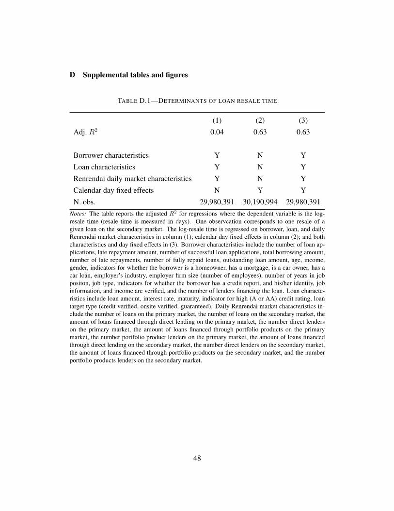
D Supplemental tables and figures

TABLE D.1—DETERMINANTS OF LOAN RESALE TIME

(1) (2) (3)

Adj. R2 0.04 0.63 0.63

Borrower characteristics Y N Y

Loan characteristics Y N Y

Renrendai daily market characteristics Y N Y

Calendar day fixed effects N Y Y

N. obs. 29,980,391 30,190,994 29,980,391Notes: The table reports the adjusted R2 for regressions where the dependent variable is the log-resale time (resale time is measured in days). One observcation corresponds to one resale of agiven loan on the secondary market. The log-resale time is regressed on borrower, loan, and dailyRenrendai market characteristics in column (1); calendar day fixed effects in column (2); and bothcharacteristics and day fixed effects in (3). Borrower characteristics include the number of loan ap-plications, late repayment amount, number of successful loan applications, total borrowing amount,number of late repayments, number of fully repaid loans, outstanding loan amount, age, income,gender, indicators for whether the borrower is a homeowner, has a mortgage, is a car owner, has acar loan, employer’s industry, employer firm size (number of employees), number of years in jobpositon, job type, indicators for whether the borrower has a credit report, and his/her identity, jobinformation, and income are verified, and the number of lenders financing the loan. Loan characte-ristics include loan amount, interest rate, maturity, indicator for high (A or AA) credit rating, loantarget type (credit verified, onsite verified, guaranteed). Daily Renrendai market characteristics in-clude the number of loans on the primary market, the number of loans on the secondary market, theamount of loans financed through direct lending on the primary market, the number direct lenderson the primary market, the amount of loans financed through portfolio products on the primarymarket, the number portfolio product lenders on the primary market, the amount of loans financedthrough direct lending on the secondary market, the number direct lenders on the secondary market,the amount of loans financed through portfolio products on the secondary market, and the numberportfolio products lenders on the secondary market.

48

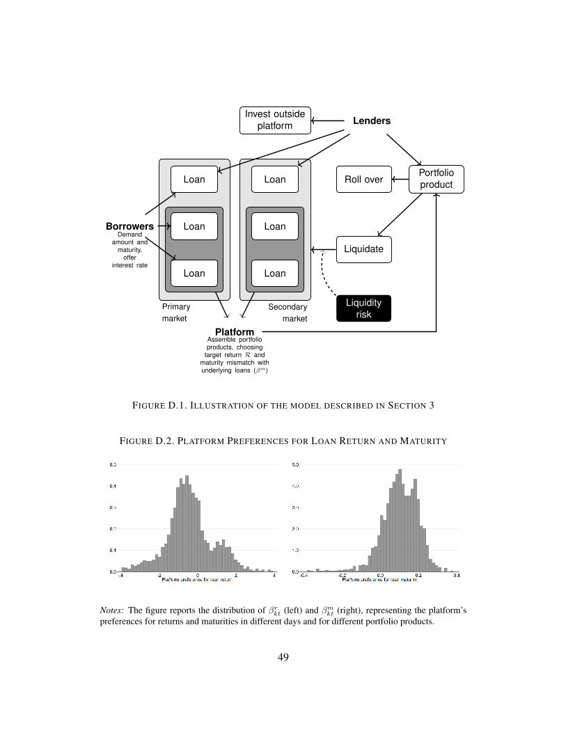
BorrowersDemand

amount andmaturity,

offerinterest rate

Primarymarket

Loan

Loan

Loan

Secondarymarket

Loan

Loan

LoanPortfolioproduct

LendersInvest outside

platform

PlatformAssemble portfolioproducts, choosing

target return R andmaturity mismatch withunderlying loans (βm)

Roll over

Liquidate

Liquidityrisk

FIGURE D.1. ILLUSTRATION OF THE MODEL DESCRIBED IN SECTION 3

FIGURE D.2. PLATFORM PREFERENCES FOR LOAN RETURN AND MATURITY

Notes: The figure reports the distribution of βrkt (left) and βmkt (right), representing the platform’spreferences for returns and maturities in different days and for different portfolio products.

49