Embed Size (px)
Citation preview
Review of Derivatives Research, 7, 241–266, 2004 2005 Kluwer Academic Publishers. Printed in the Netherlands.
The Unbiasedness Hypothesis in the FreightForward Market: Evidence from CointegrationTests
MANOLIS G. KAVUSSANOS ∗ [email protected] University of Economics and Business, 76 Patission St, TK 104 34, Athens, Greece
ILIAS D. VISVIKIS [email protected] of Piraeus, Department of Maritime Studies, 80 Karaoli & Dimitriou St, 185 34, Piraeus, Greece
DAVID MENACHOF [email protected] Business School, City University, 106 Bunhill Row, EC1Y 8TZ, London, UK
Abstract. The current paper investigates the unbiasedness hypothesis of Forward Freight Agreement (FFA)prices in the freight over-the-counter (OTC) forward market trades. Cointegration techniques are employed toexamine the hypothesis. The results indicate that: FFA prices one and two months before maturity are unbi-ased predictors of the realised spot freight rates for all investigated shipping routes; three months FFA prices forpanamax Pacific routes are unbiased predictors of spot prices, while FFA prices for panamax Atlantic routes arefound to be biased predictors of spot prices. This diverse evidence suggests that the validity of the unbiasednesshypothesis depends on the specific characteristics of the market under investigation, the selected trading routeand the time to maturity of the contract.
Keywords: forward markets, cointegration, unbiasedness, shipping.
JEL classification: G13, G14, C32
1. Introduction
According to the unbiasedness hypothesis, derivatives (futures/forward) contract pricesmust be unbiased estimators of spot prices of the underlying asset that will be realised atthe expiration date of the contract. The existence of derivatives markets therefore can helpdiscover prices, which are likely to prevail in the spot market. This paper investigates thishypothesis for the Forward Freight Agreements (FFA) market.
The aim of the formalisation (in 1992) of the FFA contract was to provide a mechanismfor hedging freight rate risk in the dry-bulk and wet-bulk sectors of the shipping industry,1
besides the Baltic International Freight Futures Exchange (BIFFEX) contract.2,3 The lat-ter was the alternative derivative contract available to agents in the shipping industry upuntil April 2002, when it ceased trading.4 Yet risk management for the agents in the ship-ping industry is very important as the sums involved are large and the volatility of freight
∗ Corresponding author.
242 KAVUSSANOS, VISVIKIS, AND MENACHOF
rates and ship prices is high, due to the strong cyclicality prevailing in these markets, seeKavussanos (2002).
To the best of our knowledge, there have not been any studies investigating the unbi-asedness hypothesis between spot and forward prices in the FFA market, due to the, untilnow, unavailability of data. A feature of this market is that the underlying commodity is aservice, which cannot be stored. The theory governing the relationship between spot andderivatives prices of continuously storable commodities is developed in Working (1970),amongst others. Thus, spot and derivatives prices for any storable commodity are thoughtto be related through a “cost-of-carry” relationship, which states that the price, at time t−n,of a derivatives contract for delivery at time t equals the price of the underlying asset attime t − n plus the total costs associated with purchasing and holding the underlying assetfrom time t − n to t . These costs include the financing costs associated with purchasingthe commodity, the storage costs (such as warehouse and insurance costs) as well as anyother costs involved in carrying the underlying asset forward in time. Mathematically, therelationship can be expressed as follows: Ft,t−n = St−n(1 + C). Where Ft,t−n is the priceof the derivatives contract at time t − n, for delivery at time t ; St−n is the spot price attime t − n; and C represents the carrying costs, expressed as a fraction of the spot price,necessary to carry the commodity forward from period t − n to the delivery date of thederivatives contract, at time t .
The cost-of-carry formula determines the price relationship between spot and derivativesprices and any deviations from this relationship will be restored in the market through risk-less arbitrage. For instance, if the derivatives price is above the cost-of-carry price thenmarket agents can exploit risk-less arbitrage profits by buying the underlying commodityand selling the derivatives contracts in what is known as the “cash-and-carry” arbitrage.Similarly, a reverse arbitrage opportunity arises when the derivatives price is below thecost-of-carry price (see (Kolb, 2000)). There are, however, a number of factors that maylead to a large deviation of spot prices from derivatives prices, thus resulting in the ex-istence of arbitrage opportunities. For instance, arbitrage opportunities may arise due tothe existence of regional supply and demand imbalances, regulatory changes, market dis-tortions created by market agents with large positions etc. Therefore, the aforementionedrelationship can be used to identify the existence of arbitrage opportunities in the market.However, in the case of spot freight rates and FFA contracts, which are written on a service(the transportation service the ship offers from port A to port B of the world, which is anon-storable commodity), the above issues do not hold, as spot and FFA prices are de-termined by supply and demand expectations and not through the cost-of-carry arbitrage.Thus, the identification of risk-less arbitrage opportunities, and therefore, market efficiencybecomes a more difficult research task.
The relationship between spot and derivatives prices for non-storable commodities isexamined in studies such as Brenner and Kroner (1995), Eydeland and Geman (1998), Ge-man and Vasicek (2001), and Bessembinder and Lemmon (2002) in the electricity deriva-tives markets. As explained above, the non-storable nature of the FFA market implies thatspot and FFA prices are not linked by a cost-of-carry (storage) relationship, as in financialand agricultural derivatives markets. Another feature of this derivative OTC market is theasymmetric transactions costs between spot and FFA markets. These costs are higher in
THE UNBIASEDNESS HYPOTHESIS IN THE FREIGHT FORWARD MARKET 243
the spot freight market (in relation to the FFA market), as it is the case for commodity spotversus futures markets.
FFA contracts are principal-to-principal contracts between a seller and a buyer to settlea freight (voyage) or hire (time-charter) rate, for a specified quantity of cargo or type ofvessel, for usually one, or a combination of the major trade routes.5 They are traded inover-the-counter (OTC) derivatives markets in any place of the world where two partiesagree to do business with each other. As trading takes place between ‘individuals’ eachparty accepts credit risk from the other party.6 To see how the process works, assume thata shipowner (or a charterer) feels that the freight market in a specific route and a specificvessel/cargo size might move against him/her. He/she approaches an approved broker tosell (buy) FFA contracts.7 The shipowner’s broker will search to find a charterer or anotherbroker who has a client with opposite expectations to the shipowner and they negotiate theterms of the contract. If an agreement is reached then the FFA contract is fixed. Settlementis made on the difference between the contracted price (forward price) and the averageprice for the route selected in the index over the last seven working days.
The FFA market is a private market in which the general public does not know that thetransaction was done. It can save money by not normally requiring initial, maintenanceand variation margins, common in the futures organised exchanges. Due to the natureof the OTC markets, there is no official institutional organisation, which assimilates allavailable information (common in futures exchanges) and reports the “best” daily pricefor the contracts. Thus, investigating whether derivatives prices informationally lead spotprices is easier in organised futures exchanges.
Several studies in the past have examined the unbiasedness hypothesis in various for-ward markets. The forward exchange rate market is investigated in studies such as those ofHakkio and Rush (1989), Barnhart and Szakmary (1991), Luintel and Paudyal (1998), Nor-rbin and Reffett (1996) and Barnhart, McNown, and Wallace (1999). Broadly, they exam-ine unbiasdness for the one-month forward exchange rates for the British pound, Germanmark, Swiss franc, Canadian dollar, French franc, US dollar and Japanese yen. The firstthree studies report evidence against unbiasdness while the last two find evidence in favourof the hypothesis. Various forward commodity prices are also investigated for unbiasdnessfor the London Metal Exchange (LME) in studies such as those of Chowdhury (1991) andMoore and Cullen (1995) and for the Commodity Exchange (COMEX) by Krehbiel andAdkins (1993). The hypothesis is rejected by the first study for quarterly lead, tin, zinc,and copper forward prices, but is not rejected by the second study for aluminium, lead,zinc, copper. The last study examines three- and four-month forward contract prices in thesilver, copper, gold and platinum market and report that unbiasedness holds only for theplatinum market. Overall then, the empirical evidence, based on cointegration techniques,is mixed; it seems that rejection or not of unbiasedness depends on the type of contract, thematurity of the contract, the market, and the time-period under investigation.
Investigation of the hypothesis for the freight forward market is interesting for the fol-lowing reasons. First, the underlying asset is a service. Second, the price discovery func-tion provides a strong and simple theory of the determination of spot prices that may prevailin the future. Third, if forward prices fulfil their price discovery role, they provide accu-rate forecasts of the realised spot prices, and consequently provide new information in the
244 KAVUSSANOS, VISVIKIS, AND MENACHOF
market and in allocating economic resources (Stein, 1981). Decisions in the physical mar-ket are thus facilitated and can help secure market agents’ cash-flow (transportation costs).On the other hand, the existence of inefficiency of forward prices in marking spot pricescan increase the cost of hedging, assuming that the market agents are fully informed whenthey set the forward price in FFA contracts.8 However, it must be noted that market agentscan initiate trade for several motives, such as heterogeneous expectations or heterogeneousincome/cost structures (Calvet, Gonzalez-Eiras, and Sodini, 2004). Finally, the apparentlack of research in the freight forward trades further motivates this investigation as this isthe only derivative instrument available to agents in the bulk shipping industry for hedgingpurposes. Evidence on whether agents in the shipping industry can use FFAs of differ-ent maturities and for different routes, as unbiased predictors of spot freight rates, is veryimportant and provides a free source of information for decision-making.
The remainder of this paper is organised as follows. Section two presents the methodol-ogy for testing the unbiasedness hypothesis. Section three takes a preliminary look at thedata and tests their statistical properties. Section four applies the cointegration methodsto the FFA freight derivatives market and tests the unbiasedness hypothesis. Section fivediscusses the results, while the last section concludes the paper.
2. The Unbiasedness Hypothesis and Cointegration
Theoretically, a forward price is equivalent to the expected spot price at maturity, underthe joint hypothesis of no risk-premium and rational use of information.9 The relationshipcan be tested empirically through the following equation (see, for example, (Moore andCullen, 1995; Barnhart, McNown, and Wallace, 1999)):
St = β1 + β2Ft,t−n + ut ; ut ∼ iid(0, σ 2), (1)
where Ft,t−n is the forward price at time t − n, for delivery at time t , St is the spot priceat the maturity of the contract and ut is a white noise error process. Unbiasedness holdswhen the following parameter restrictions (β1, β2) = (0, 1) are valid.
Because most macroeconomic (time series) variables are found to be non-stationary(they have a unit root) use of ordinary least squares (OLS) to estimate Equation (1), resultin inconsistent coefficient estimates and t- and F -statistics which do not follow standarddistributions (Granger and Newbold, 1974). The cointegration framework, developed byEngle and Granger (1987) and Johansen (1988, 1991) can be used to resolve the prob-lem and reliably test for unbiasedness.10 Engle and Granger (1987) demonstrate that iftwo non-stationary variables are cointegrated, the variables follow a well-specified error-correction model (ECM), where the coefficient estimates, as well as the standard errors ofthe coefficients are consistent.
The following vector error correction modelling (VECM) framework, proposed by Jo-hansen (1988), is used to test for unbiasedness:
�Xt = µ +p−1∑
i=1
�i�Xt−i + �Xt−1 + εt ; εt ∼ N(0,�), (2)
THE UNBIASEDNESS HYPOTHESIS IN THE FREIGHT FORWARD MARKET 245
where Xt is the 2 × 1 vector (St , Ft,t−n)′, µ is a 2 × 1 vector of deterministic components
which may include a linear trend term, an intercept term, or both, � denotes the first differ-ence operator, εt is a 2 × 1 vector of residuals (uS,t , uF,t )
′ and � the variance/covariancematrix of the latter. The VECM specification contains information on both the short- andlong-run adjustment to changes in Xt , via the estimates of �i and �, respectively.
Johansen and Juselius (1990), show that the coefficient matrix � contains the essentialinformation about cointegration between St and Ft,t−n. If rank(�) = 0, then � is 2 × 2zero matrix implying that there is no cointegrating relationship between St and Ft,t−n. Inthis case the VECM reduces to a Vector Autoregressive (VAR) model in first differences. If� has a full rank, that is rank(�) = 2, then all variables in Xt are I (0) and the appropriatemodelling strategy is to estimate a VAR model in levels. If � has a reduced rank, that isrank(�) = 1, then there is a single cointegration relationship between St and Ft,t−n andthe expression �Xt−1 is the error correction term. In this case, � can be factored intotwo 2 × 1 matrices a and β: � = aβ ′, where β ′ represents the vector of cointegratingparameters and α is the vector of error correction coefficients, measuring the speed ofconvergence to the long-run steady state.
Since rank(�) equals the number of characteristic roots (or eigenvalues) which are dif-ferent from zero, the number of distinct cointegration vectors can be obtained by estimatingthe number of these eigenvalues, which are significantly different from zero. The charac-teristic roots of the q ×q matrix �, are the values of λ which satisfy the following equation|� − λIq | = 0, where Iq is a q × q identity matrix.11
The choice of the deterministic components that should be included in the VECM is im-portant since the asymptotic distributions of the cointegration test statistics are dependentupon the presence of trends and/or constants in the VECM and is a task that must be sup-ported by some economic argument.12 Unbiasedness is tested by the following restrictionsβ1 = 0 and β2 = −1 on the cointegrating vector. The following statistic proposed byJohansen and Juselius (1990) may be used for that:
−T[ln
(1 − λ̂∗
1
) − ln(1 − λ̂1
)] ∼ χ2(2), (3)
where λ̂1 is the largest eigenvalue of the unrestricted model and λ̂∗1 is the largest eigenvalue
of the model with the imposed restrictions on the cointegrating vector. The asymptoticdistribution of the likelihood ratio test statistic is χ2 with degrees of freedom equal to thenumber of assumed parameter restrictions (r) placed on β ′.
The Fully Modified Least Squares (FM-LS) cointegration test, proposed by Phillips andHansen (1990), and the Bierens (1997) non-parametric test can also be used to test forunbiasedness. Their use is motivated by the overlapping observations problem, present inthe two- and three-months maturity periods, which may affect the Johansen (1988) test(Hansen and Hodrick, 1980). With overlapping contract periods, if the observation fre-quency of the sample data is, say h, where h < n (n is the maturity of the contract) inEquation (1), a moving average process of order n/h − 1 in the residuals may be gener-ated.
The Phillips and Hansen (1990) method applies a non-parametric correction to the OLScoefficient estimates and to their associated t-statistics to take into account the impact ofautocorrelation on the residual term when the right-hand side variables of Equation (1) are
246 KAVUSSANOS, VISVIKIS, AND MENACHOF
not weakly exogenous. The Phillips and Hansen (1990) method leads to fully modifiedestimates of both parameters and standard errors, which are asymptotically equivalent tomaximum likelihood estimates.13 The method of Phillips and Hansen (1990) does not suf-fer from the overlapping observations problem, since it only involves an adjustment to theOLS estimates of the cointegration vector without any reliance on the parameters govern-ing the short-run dynamics (the estimate of the long-run covariance is positive definite inevery case).
Bierens (1997) proposes a multivariate non-parametric method of estimation of Equa-tion (1), which is in the same spirit as Johansen’s method in that the test statistics areobtained from the solutions of a generalised eigenvalue problem and the hypotheses to betested are the same. Their main important difference is that the Bierens method estimatestwo random matrices, in the generalised eigenvalue problem, constructed independentlyof the data generating process. These matrices consist of weighted means of the sys-tem variables in levels and first differences and are constructed such that their generalisedeigenvalues share similar properties to those in the Johansen method.14 In contrast, theJohansen’s (1991) method constructs the (q × q) � matrix to be dependent on the datagenerating process in a parametric way.
3. Description of the Data and Their Statistical Properties
From the formulation of the FFA market on February 1st 1992 until November 1st 1999,the eleven panamax and capesize voyage and time-charter routes of the Baltic FreightIndex (BFI) served as the underlying assets of the FFA trades, in the dry-bulk sector ofthe shipping industry. After the latter date, with the exclusion of the capesize routes andwith the renamed index as BPI, the underlying assets of the FFA contracts are panamaxroutes. The composition of the BPI, as it stands on January 2001, is presented in Table 1.
Data for FFA rates on four panamax routes, namely routes 1, 1A, 2, and 2A, and threecontract maturities – one-, two-, and three-months, are obtained from Clarkson Securitiesfor the period 1996:01–2000:12.15 The reason for using only four routes out of seven, andJanuary 1996 as a starting date (instead of 1992), is due to the lack of FFA quotes of ship-brokers for the remaining routes (3, 3A, and 4) and for the years 1992–1995, respectively.It should also be noted that not all the investigated shipping routes attract high interest forFFA trading. Routes 1 and 1A fall in this category and as a result shipbrokers have stoppedpublishing daily FFA quotes for those routes (still if a market agent is interested in tradingon those routes, then shipbrokers can accommodate this need and draft a FFA contract).For instance, shipping routes located on the Pacific region (see Table 1 for more details)attract more than 80 percent of paper (FFA) trade according to market estimates, whereaspaper trade on shipping routes located on the Atlantic region is very modest. The reasonfor this phenomenon may be attributed to the historical increased interest of market agentsfor the spot (underlying) Pacific markets. Moreover, the correlation between spot and FFAPacific prices is higher than the relevant correlation between spot and FFA Atlantic prices.Hence, FFA prices for those routes may not incorporate new information at the same rateand/or quality as the other two investigated routes – routes 2 and 2A. A priori, unbiased-
THE UNBIASEDNESS HYPOTHESIS IN THE FREIGHT FORWARD MARKET 247
Table 1. Baltic Panamax Index (BPI)—Route, Cargo type and Vessel Size Definitions
Routes Route Description CARGO Vessel WeightingsSize (dwt) in BPI
1 1–2 safe berths/anchorages US Gulf (MississippiRiver not above Baton Rouge) to ARA (Antwerp,Rotterdam, Amsterdam).
Light Grain 55,000 10%
1A Transatlantic (including East Coast of South Amer-ica) round of 45–60 days on the basis of delivery andredelivery Skaw Passero range.
T/C 70,000 20%
2 1–2 safe berths/anchorages US Gulf (MississippiRiver not above Baton Rouge) / 1 no combo port toSouth Japan.
HSS 54,000 12.5%
2A Basis delivery Skaw Passero range, for a trip via Gulfto the Far East, redelivery Taiwan–Japan range, dura-tion 50–60 days.
T/C 70,000 12.5%
3 1 port US North Pacific / 1 no combo port to SouthJapan.
HSS 54,000 10%
3A Transpacific round of 35–50 days either via Australiaor Pacific (but not including short rounds such asVostochy/Japan), delivery and redelivery Japan/SouthKorea range.
T/C 70,000 20%
4 Delivery Japan/South Korea range for a trip via USWest Coast–British Columbia range, redelivery Skawrange, duration 50–60 days.
T/C 70,000 15%
Source: Baltic Exchange.Notes:
• From the formulation of the FFA market on February 1st 1992 until November 1st 1999, the eleven panamaxand capesize voyage and time-charter routes of the Baltic Freight Index (BFI) served as the underlying assetsof the FFA trades, in the dry-bulk sector of the shipping industry. After the latter date, with the exclusion ofthe capesize routes and with the renamed index as Baltic Panamax Index (BPI), the underlying assets of theFFA contracts are panamax routes. The composition of the BPI, as it stands on January 2001, is presented inthe table.
• In the first column of the table the different Panamax shipping routes are presented. Routes 1–4 are voyageshipping routes (which involve the carriage of cargo between specified ports for a predetermined freight rate),and routes 1A–3A are time-charter shipping routes (under which a shipowner agrees to hire out the vessel toa charterer (a party with cargo to transport) for a specified period of time, providing crew together with thevessel, voyage costs being paid by the charterer in this case).
• In the second column of the table the description of each of the seven shipping routes is presented.• In the third column of the table the cargos that are transported under each shipping route are presented. T/C
refers to Time-charter contracts. HSS stands for Heavy Grain, Soya and Sorghum.• In the fourth column of the table the vessel size is presented, which is measured by the carrying capacity of the
vessel (dwt—deadweight tones) and includes the effective cargo, bunkers, lubricants, water, food rations, crewand any passengers.
• In the fifth column of the table the individual weight of each route in the BPI is presented. When calculatingthe BPI each shipping route is given an individual weighting to reflect its importance in the worldwide freightmarket.
• Skaw Passero refers to the area that extends from Cape Skaw in Denmark to Cape Passero in Sicily (Italy).
248 KAVUSSANOS, VISVIKIS, AND MENACHOF
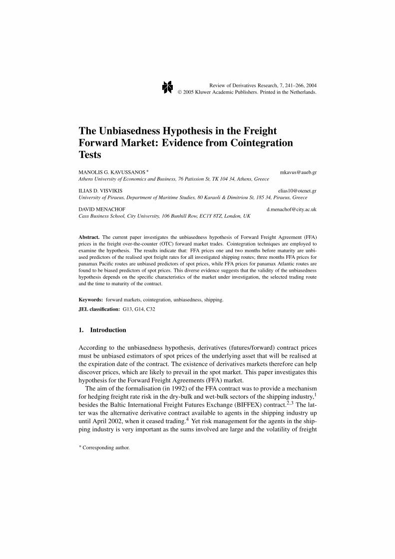
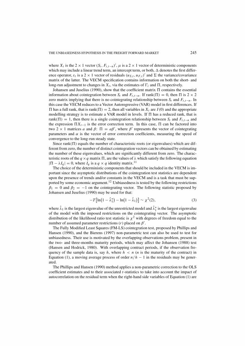
Figure 1. Spot freight rates (spot in $/ton) and one-month Forward Freight Agreement (FFA in $/ton) prices forRoute 1. Notes: The data sets used are spot freight rates and one-month FFA prices for Route 1 (US Gulf to ARA(Antwerp, Rotterdam, Amsterdam), expressed in $/ton). The FFA price series are the average (mid-point) of bidand offer quotes and are obtained from Clarkson Securities Ltd. Data for spot freight rates are obtained fromDatastream for the period 1996:01–2000:12. FFA prices are matched with realised spot prices at the contractmaturity (or prompt) date. The prompt date is normally the last trading day of each month, except for theDecember contract, which is the 20th of the month. If the prompt date falls on a non-business day, i.e., a Sundayor a holiday, it is relocated to the next available business day.
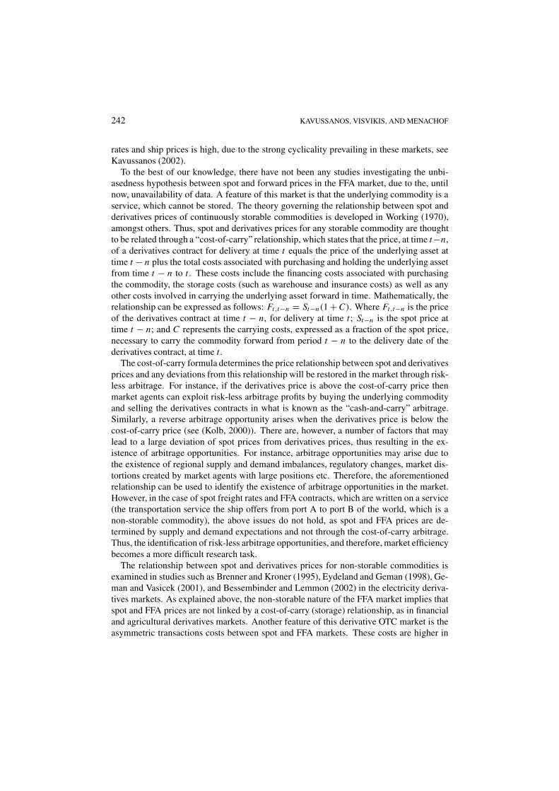
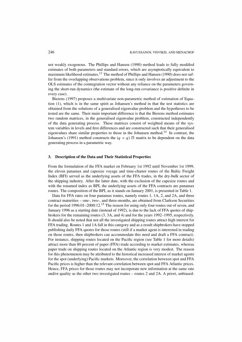
Figure 2. Spot freight rates (spot in $/ton) and two-months Forward Freight Agreement (FFA in $/ton) pricesfor Route 1. Notes: The data sets used are monthly spot freight rates and two-months FFA prices for Route 1.See also notes in Figure 1.
ness is expected to hold relatively well in a well functioning and liquid forward marketsin comparison to the less liquid ones. This has a bearing on the results presented in thesubsequent parts of the paper.
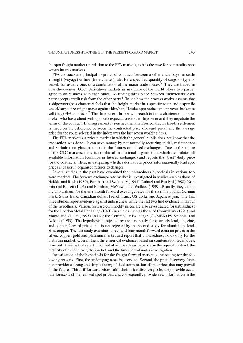
The FFA price series are the average (mid-point) of bid and offer quotes (as in(Moore and Cullen, 1995; Evans and Lewis, 1995; Luintel and Paudyal, 1998)). Datafor spot freight rates for the same routes are obtained from Datastream for the period1996:01–2000:12. To get an idea of what the data look like, the spot and FFA time se-ries for route 1, for the three contract maturities are shown in Figures 1–3. The rest of theseries are not shown in order to conserve space.
THE UNBIASEDNESS HYPOTHESIS IN THE FREIGHT FORWARD MARKET 249
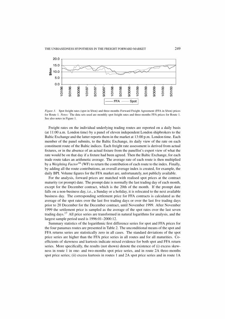
Figure 3. Spot freight rates (spot in $/ton) and three-months Forward Freight Agreement (FFA in $/ton) pricesfor Route 1. Notes: The data sets used are monthly spot freight rates and three-months FFA prices for Route 1.See also notes in Figure 1.
Freight rates on the individual underlying trading routes are reported on a daily basis(at 11:00 a.m. London time) by a panel of eleven independent London shipbrokers to theBaltic Exchange and the latter reports them in the market at 13:00 p.m. London time. Eachmember of the panel submits, to the Baltic Exchange, its daily view of the rate on eachconstituent route of the Baltic indices. Each freight rate assessment is derived from actualfixtures, or in the absence of an actual fixture from the panellist’s expert view of what therate would be on that day if a fixture had been agreed. Then the Baltic Exchange, for eachtrade route takes an arithmetic average. The average rate of each route is then multipliedby a Weighting Factor16 (WF) to return the contribution of each route to the index. Finally,by adding all the route contributions, an overall average index is created, for example, thedaily BPI. Volume figures for the FFA market are, unfortunately, not publicly available.
For the analysis, forward prices are matched with realised spot prices at the contractmaturity (or prompt) date. The prompt date is normally the last trading day of each month,except for the December contract, which is the 20th of the month. If the prompt datefalls on a non-business day, i.e., a Sunday or a holiday, it is relocated to the next availablebusiness day. The corresponding settlement price for FFA contracts is calculated as theaverage of the spot rates over the last five trading days or over the last five trading daysprior to 20 December for the December contract, until November 1999. After November1999 the settlement price is sampled as the average of the spot rates over the last seventrading days.17 All price series are transformed in natural logarithms for analysis, and thelargest sample period used is 1996:01–2000:12.
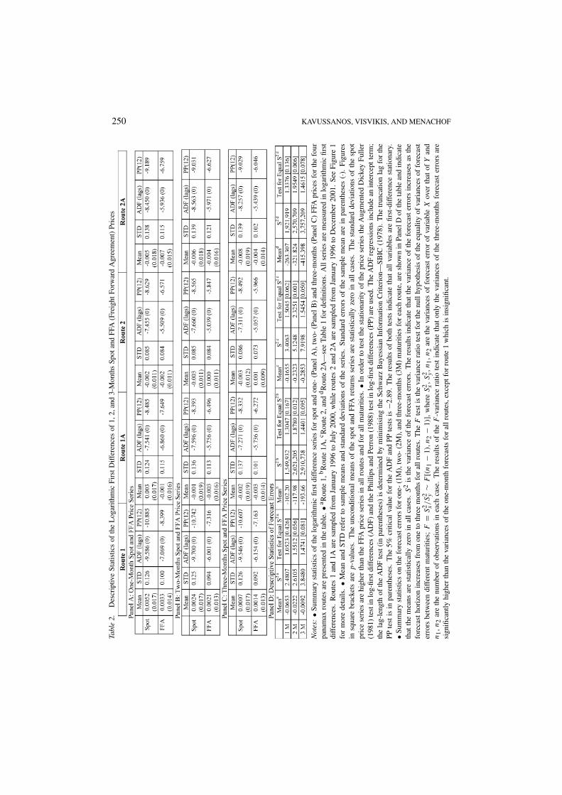
Summary statistics of the logarithmic first difference series for spot and FFA prices forthe four panamax routes are presented in Table 2. The unconditional means of the spot andFFA returns series are statistically zero in all cases. The standard deviations of the spotprice series are higher than the FFA price series in all routes and for all maturities. Co-efficients of skewness and kurtosis indicate mixed evidence for both spot and FFA returnseries. More specifically, the results (not shown) denote the existence of (i) excess skew-ness in route 1 in one- and two-months spot price series, and in route 2A three-monthsspot price series; (ii) excess kurtosis in routes 1 and 2A spot price series and in route 1A
250 KAVUSSANOS, VISVIKIS, AND MENACHOF
Tabl
e2.
Des
crip
tive
Stat
istic
sof
the
Log
arith
mic
Firs
tDif
fere
nces
of1,
2,an
d3-
Mon
ths
Spot
and
FFA
(Fre
ight
Forw
ard
Agr
eem
ent)
Pric
es
Not
es:
•Sum
mar
yst
atis
tics
ofth
elo
gari
thm
icfir
stdi
ffer
ence
seri
esfo
rsp
otan
don
e-(P
anel
A),
two-
(Pan
elB
)an
dth
ree-
mon
ths
(Pan
elC
)FF
Apr
ices
for
the
four
pana
max
rout
esar
epr
esen
ted
inth
eta
ble.
•a Rou
te1,
bR
oute
1A,c R
oute
2,an
ddR
oute
2A—
see
Tabl
e1
for
defin
ition
s.A
llse
ries
are
mea
sure
din
loga
rith
mic
first
diff
eren
ces.
Rou
tes
1an
d1A
are
sam
pled
from
Janu
ary
1996
toJu
ly20
00,w
hile
rout
es2
and
2Aar
esa
mpl
edfr
omJa
nuar
y19
96to
Dec
embe
r20
01.
See
Figu
re1
for
mor
ede
tails
.•M
ean
and
STD
refe
rto
sam
ple
mea
nsan
dst
anda
rdde
viat
ions
ofth
ese
ries
.St
anda
rder
rors
ofth
esa
mpl
em
ean
are
inpa
rent
hese
s(·)
.Fi
gure
sin
squa
rebr
acke
tsar
ep
-val
ues.
The
unco
nditi
onal
mea
nsof
the
spot
and
FFA
retu
rns
seri
esar
est
atis
tical
lyze
roin
all
case
s.T
hest
anda
rdde
viat
ions
ofth
esp
otpr
ice
seri
esar
ehi
gher
than
the
FFA
pric
ese
ries
inal
lrou
tes
and
for
allm
atur
ities
.•I
nor
der
tote
stth
est
atio
nari
tyof
the
pric
ese
ries
the
Aug
men
ted
Dic
key
Fulle
r(1
981)
test
inlo
g-fir
stdi
ffer
ence
s(A
DF)
and
the
Phill
ips
and
Perr
on(1
988)
test
inlo
g-fir
stdi
ffer
ence
s(P
P)ar
eus
ed.T
heA
DF
regr
essi
ons
incl
ude
anin
terc
eptt
erm
;th
ela
g-le
ngth
ofth
eA
DF
test
(in
pare
nthe
ses)
isde
term
ined
bym
inim
isin
gth
eSc
hwar
zB
ayes
sian
Info
rmat
ion
Cri
teri
on—
SBIC
(197
8).
The
trun
catio
nla
gfo
rth
ePP
test
isin
pare
nthe
ses.
The
5%cr
itica
lva
lue
for
the
AD
Fan
dPP
test
sis
−2.8
9.T
here
sults
ofbo
thte
sts
indi
cate
that
all
vari
able
sar
efir
st-d
iffe
renc
est
atio
nary
.•S
umm
ary
stat
istic
son
the
fore
cast
erro
rsfo
ron
e-(1
M),
two-
(2M
),an
dth
ree-
mon
ths
(3M
)m
atur
ities
for
each
rout
e,ar
esh
own
inPa
nelD
ofth
eta
ble
and
indi
cate
that
the
mea
nsar
est
atis
tical
lyze
roin
allc
ases
.S
2is
the
vari
ance
ofth
efo
reca
ster
rors
.T
here
sults
indi
cate
that
the
vari
ance
ofth
efo
reca
ster
rors
incr
ease
sas
the
fore
cast
hori
zon
incr
ease
sfr
omon
eto
thre
em
onth
sfo
ral
lrou
tes.
The
Fte
stis
the
vari
ance
ratio
test
for
the
null
hypo
thes
isof
the
equa
lity
ofva
rian
ces
offo
reca
ster
rors
betw
een
diff
eren
tm
atur
ities
;F
=S
2 x/S
2 y∼
F[(n
1−
1),n
2−
1)],w
here
S2 x,S
2 y,n
1,n
2ar
eth
eva
rian
ces
offo
reca
ster
ror
ofva
riab
leX
over
that
ofY
and
n1,n
2ar
eth
enu
mbe
rof
obse
rvat
ions
inea
chca
se.
The
resu
ltsof
the
F-v
aria
nce
ratio
test
indi
cate
that
only
the
vari
ance
sof
the
thre
e-m
onth
sfo
reca
ster
rors
are
sign
ifica
ntly
high
erth
anth
eva
rian
ces
ofth
eon
e-m
onth
fore
cast
sfo
ral
lrou
tes,
exce
ptfo
rro
ute
1w
hich
isin
sign
ifica
nt.
THE UNBIASEDNESS HYPOTHESIS IN THE FREIGHT FORWARD MARKET 251
three-months FFA price series; Jarque–Bera (1981) tests indicate that, with the exceptionof routes 1 and 2A spot prices and route 1A three-months FFA prices, the return seriesfollow normal distributions.
Results of the Augmented Dickey–Fuller (ADF) (Dickey and Fuller, 1981) and Phillips–Perron (1988) tests, in the same table, indicate that all variables are first-difference station-ary. ADF and PP tests are criticised for lack of power in rejecting the null hypothesis ofa unit root when it is false (Lee, Gleason, and Mathur, 2000). This lack of power is ad-dressed by the KPSS test proposed by Kwiatkowski et al. (1992), which has stationarity asthe null hypothesis.18 However, results from applying the KPSS test for the series confirmthe ADF and PP test findings.
Summary statistics on the forecast errors for one-, two-, and three-months maturities foreach route, shown in Panel D of the same table, indicate that their means are statisticallyzero in all cases. It seems that the variance of the forecast errors increases as the forecasthorizon increases from one to three months for all routes. The results of applying anF -variance ratio test to examine the above inference indicate that only the variances of thethree-months forecast errors are significantly higher than the variances of the one-monthforecasts for all routes, except for route 1 which is insignificant. Due to the small samplesize, we apply a bootstrap procedure to confirm the above findings, which yields the sameresults (not shown). These findings are in line with Samuelson (1965) who argued that thevolatility of a derivatives contract is a negative function of its time to maturity.
4. Empirical Results
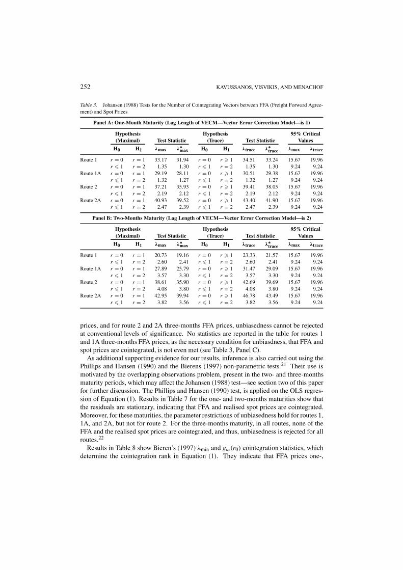
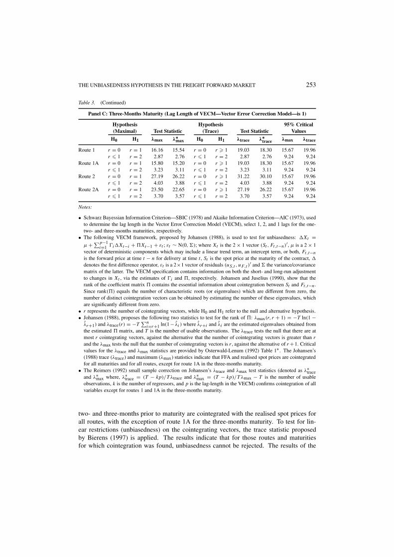
Having identified that spot and FFA prices are I (1) variables, Table 3 presents resultswhich test for cointegration of these series. Schwarz Bayessian Information Criterion(SBIC) (Schwartz, 1978) and Akaike Information Criterion (AIC) (Akaike, 1973), used todetermine the lag length in the VECM, select 1, 2, and 1 lags for the one-, two- and three-months maturities, respectively.19 Use of the Johansen (1991) LR test of Equation (5)select a restricted intercept in the cointegration vector in all cases. The Johansen’s (1988)trace (λtrace) and maximum (λmax) statistics of Equations (3) and (4), in Table 3, indicatethat FFA and realised spot prices are cointegrated for all maturities and for all routes, exceptfor route 1A in the three-months maturity. The Reimers (1992) small sample correction onJohansen’s λtrace and λmax test statistics (denoted as λ∗
trace and λ∗max) confirms cointegration
of all variables except for routes 1 and 1A in the three-months maturity.20 Therefore in theensuing analysis, for routes 1 and 1A investigation for unbiasedness comes to an end asthe necessary condition of cointegration is not satisfied.
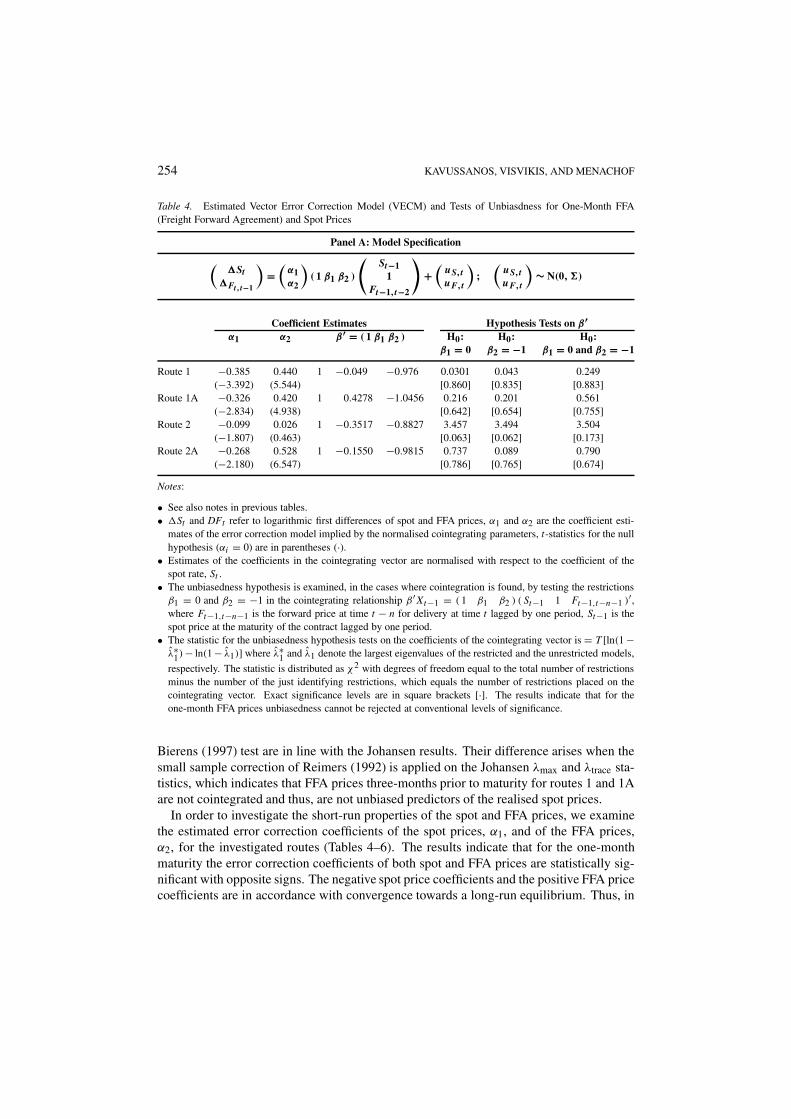
The unbiasedness hypothesis is examined next, in the cases where cointegration isfound, by testing the restrictions β1 = 0 and β2 = −1 in the cointegrating relationshipβ ′Xt−1 = (1 β1 β2)(St−1 1 Ft−1,t−n−1)
′. If these restrictions hold, then the price of theFFA contract is an unbiased predictor of the realised spot price. The estimated coefficientsof the cointegrating vectors, the hypothesis tests on β ′ using Equation (3), along with theresidual diagnostics of the models, are presented in Tables 4–6 for the one-, two- and three-months maturities, respectively. The results indicate that for the one- and two-months FFA
252 KAVUSSANOS, VISVIKIS, AND MENACHOF
Table 3. Johansen (1988) Tests for the Number of Cointegrating Vectors between FFA (Freight Forward Agree-ment) and Spot Prices
Panel A: One-Month Maturity (Lag Length of VECM—Vector Error Correction Model—is 1)
Hypothesis Hypothesis 95% Critical(Maximal) Test Statistic (Trace) Test Statistic Values
H0 H1 λmax λ∗max H0 H1 λtrace λ∗
trace λmax λtrace
Route 1 r = 0 r = 1 33.17 31.94 r = 0 r � 1 34.51 33.24 15.67 19.96r � 1 r = 2 1.35 1.30 r � 1 r = 2 1.35 1.30 9.24 9.24
Route 1A r = 0 r = 1 29.19 28.11 r = 0 r � 1 30.51 29.38 15.67 19.96r � 1 r = 2 1.32 1.27 r � 1 r = 2 1.32 1.27 9.24 9.24
Route 2 r = 0 r = 1 37.21 35.93 r = 0 r � 1 39.41 38.05 15.67 19.96r � 1 r = 2 2.19 2.12 r � 1 r = 2 2.19 2.12 9.24 9.24
Route 2A r = 0 r = 1 40.93 39.52 r = 0 r � 1 43.40 41.90 15.67 19.96r � 1 r = 2 2.47 2.39 r � 1 r = 2 2.47 2.39 9.24 9.24
Panel B: Two-Months Maturity (Lag Length of VECM—Vector Error Correction Model—is 2)
Hypothesis Hypothesis 95% Critical(Maximal) Test Statistic (Trace) Test Statistic Values
H0 H1 λmax λ∗max H0 H1 λtrace λ∗
trace λmax λtrace
Route 1 r = 0 r = 1 20.73 19.16 r = 0 r � 1 23.33 21.57 15.67 19.96r � 1 r = 2 2.60 2.41 r � 1 r = 2 2.60 2.41 9.24 9.24
Route 1A r = 0 r = 1 27.89 25.79 r = 0 r � 1 31.47 29.09 15.67 19.96r � 1 r = 2 3.57 3.30 r � 1 r = 2 3.57 3.30 9.24 9.24
Route 2 r = 0 r = 1 38.61 35.90 r = 0 r � 1 42.69 39.69 15.67 19.96r � 1 r = 2 4.08 3.80 r � 1 r = 2 4.08 3.80 9.24 9.24
Route 2A r = 0 r = 1 42.95 39.94 r = 0 r � 1 46.78 43.49 15.67 19.96r � 1 r = 2 3.82 3.56 r � 1 r = 2 3.82 3.56 9.24 9.24
prices, and for route 2 and 2A three-months FFA prices, unbiasedness cannot be rejectedat conventional levels of significance. No statistics are reported in the table for routes 1and 1A three-months FFA prices, as the necessary condition for unbiasdness, that FFA andspot prices are cointegrated, is not even met (see Table 3, Panel C).
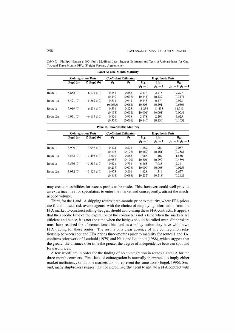
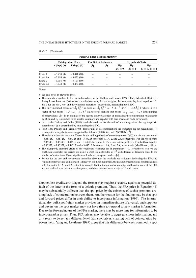
As additional supporting evidence for our results, inference is also carried out using thePhillips and Hansen (1990) and the Bierens (1997) non-parametric tests.21 Their use ismotivated by the overlapping observations problem, present in the two- and three-monthsmaturity periods, which may affect the Johansen (1988) test—see section two of this paperfor further discussion. The Phillips and Hansen (1990) test, is applied on the OLS regres-sion of Equation (1). Results in Table 7 for the one- and two-months maturities show thatthe residuals are stationary, indicating that FFA and realised spot prices are cointegrated.Moreover, for these maturities, the parameter restrictions of unbiasedness hold for routes 1,1A, and 2A, but not for route 2. For the three-months maturity, in all routes, none of theFFA and the realised spot prices are cointegrated, and thus, unbiasedness is rejected for allroutes.22
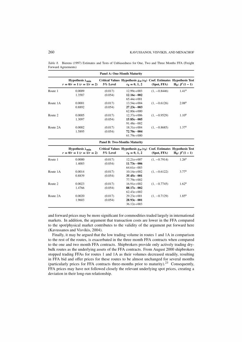
Results in Table 8 show Bieren’s (1997) λmin and gm(r0) cointegration statistics, whichdetermine the cointegration rank in Equation (1). They indicate that FFA prices one-,
THE UNBIASEDNESS HYPOTHESIS IN THE FREIGHT FORWARD MARKET 253
Table 3. (Continued)
Panel C: Three-Months Maturity (Lag Length of VECM—Vector Error Correction Model—is 1)
Hypothesis Hypothesis 95% Critical(Maximal) Test Statistic (Trace) Test Statistic Values
H0 H1 λmax λ∗max H0 H1 λtrace λ∗
trace λmax λtrace
Route 1 r = 0 r = 1 16.16 15.54 r = 0 r � 1 19.03 18.30 15.67 19.96r � 1 r = 2 2.87 2.76 r � 1 r = 2 2.87 2.76 9.24 9.24
Route 1A r = 0 r = 1 15.80 15.20 r = 0 r � 1 19.03 18.30 15.67 19.96r � 1 r = 2 3.23 3.11 r � 1 r = 2 3.23 3.11 9.24 9.24
Route 2 r = 0 r = 1 27.19 26.22 r = 0 r � 1 31.22 30.10 15.67 19.96r � 1 r = 2 4.03 3.88 r � 1 r = 2 4.03 3.88 9.24 9.24
Route 2A r = 0 r = 1 23.50 22.65 r = 0 r � 1 27.19 26.22 15.67 19.96r � 1 r = 2 3.70 3.57 r � 1 r = 2 3.70 3.57 9.24 9.24
Notes:
• Schwarz Bayessian Information Criterion—SBIC (1978) and Akaike Information Criterion—AIC (1973), usedto determine the lag length in the Vector Error Correction Model (VECM), select 1, 2, and 1 lags for the one-two- and three-months maturities, respectively.
• The following VECM framework, proposed by Johansen (1988), is used to test for unbiasedness: �Xt =µ + ∑p−1
i=1 �i�Xt−i + �Xt−1 + εt ; εt ∼ N(0, �); where Xt is the 2 × 1 vector (St , Ft,t−n)′, µ is a 2 × 1vector of deterministic components which may include a linear trend term, an intercept term, or both, Ft,t−n
is the forward price at time t − n for delivery at time t , St is the spot price at the maturity of the contract, �
denotes the first difference operator, εt is a 2×1 vector of residuals (uS,t , uF,t )′ and � the variance/covariance
matrix of the latter. The VECM specification contains information on both the short- and long-run adjustmentto changes in Xt , via the estimates of �i and �, respectively. Johansen and Juselius (1990), show that therank of the coefficient matrix � contains the essential information about cointegration between St and Ft,t−n.Since rank(�) equals the number of characteristic roots (or eigenvalues) which are different from zero, thenumber of distinct cointegration vectors can be obtained by estimating the number of these eigenvalues, whichare significantly different from zero.
• r represents the number of cointegrating vectors, while H0 and H1 refer to the null and alternative hypothesis.• Johansen (1988), proposes the following two statistics to test for the rank of �: λmax(r, r + 1) = −T ln(1 −
λ̂r+1) and λtrace(r) = −T∑n
i=r+1 ln(1− λ̂i ) where λ̂r+i and λ̂i are the estimated eigenvalues obtained fromthe estimated � matrix, and T is the number of usable observations. The λtrace tests the null that there are atmost r cointegrating vectors, against the alternative that the number of cointegrating vectors is greater than r
and the λmax tests the null that the number of cointegrating vectors is r , against the alternative of r +1. Criticalvalues for the λtrace and λmax statistics are provided by Osterwald-Lenum (1992) Table 1∗. The Johansen’s(1988) trace (λtrace) and maximum (λmax) statistics indicate that FFA and realised spot prices are cointegratedfor all maturities and for all routes, except for route 1A in the three-months maturity.
• The Reimers (1992) small sample correction on Johansen’s λtrace and λmax test statistics (denoted as λ∗trace
and λ∗max where, λ∗
trace = (T − kp)/T λtrace and λ∗max = (T − kp)/T λmax − T is the number of usable
observations, k is the number of regressors, and p is the lag-length in the VECM) confirms cointegration of allvariables except for routes 1 and 1A in the three-months maturity.
two- and three-months prior to maturity are cointegrated with the realised spot prices forall routes, with the exception of route 1A for the three-months maturity. To test for lin-ear restrictions (unbiasedness) on the cointegrating vectors, the trace statistic proposedby Bierens (1997) is applied. The results indicate that for those routes and maturitiesfor which cointegration was found, unbiasedness cannot be rejected. The results of the
254 KAVUSSANOS, VISVIKIS, AND MENACHOF
Table 4. Estimated Vector Error Correction Model (VECM) and Tests of Unbiasdness for One-Month FFA(Freight Forward Agreement) and Spot Prices
Panel A: Model Specification
(�St
�Ft,t−1
)=
(α1α2
)( 1 β1 β2 )
St−1
1Ft−1,t−2
+
(uS,t
uF,t
);
(uS,t
uF,t
)∼ N(0,�)
Coefficient Estimates Hypothesis Tests on β ′α1 α2 β ′ = ( 1 β1 β2 ) H0: H0: H0:
β1 = 0 β2 = −1 β1 = 0 and β2 = −1
Route 1 −0.385 0.440 1 −0.049 −0.976 0.0301 0.043 0.249(−3.392) (5.544) [0.860] [0.835] [0.883]
Route 1A −0.326 0.420 1 0.4278 −1.0456 0.216 0.201 0.561(−2.834) (4.938) [0.642] [0.654] [0.755]
Route 2 −0.099 0.026 1 −0.3517 −0.8827 3.457 3.494 3.504(−1.807) (0.463) [0.063] [0.062] [0.173]
Route 2A −0.268 0.528 1 −0.1550 −0.9815 0.737 0.089 0.790(−2.180) (6.547) [0.786] [0.765] [0.674]
Notes:
• See also notes in previous tables.• �St and DFt refer to logarithmic first differences of spot and FFA prices, α1 and α2 are the coefficient esti-
mates of the error correction model implied by the normalised cointegrating parameters, t-statistics for the nullhypothesis (αi = 0) are in parentheses (·).
• Estimates of the coefficients in the cointegrating vector are normalised with respect to the coefficient of thespot rate, St .
• The unbiasedness hypothesis is examined, in the cases where cointegration is found, by testing the restrictionsβ1 = 0 and β2 = −1 in the cointegrating relationship β ′Xt−1 = ( 1 β1 β2 ) ( St−1 1 Ft−1,t−n−1 )′,where Ft−1,t−n−1 is the forward price at time t − n for delivery at time t lagged by one period, St−1 is thespot price at the maturity of the contract lagged by one period.
• The statistic for the unbiasedness hypothesis tests on the coefficients of the cointegrating vector is = T [ln(1 −λ̂∗
1) − ln(1 − λ̂1)] where λ̂∗1 and λ̂1 denote the largest eigenvalues of the restricted and the unrestricted models,
respectively. The statistic is distributed as χ2 with degrees of freedom equal to the total number of restrictionsminus the number of the just identifying restrictions, which equals the number of restrictions placed on thecointegrating vector. Exact significance levels are in square brackets [·]. The results indicate that for theone-month FFA prices unbiasedness cannot be rejected at conventional levels of significance.
Bierens (1997) test are in line with the Johansen results. Their difference arises when thesmall sample correction of Reimers (1992) is applied on the Johansen λmax and λtrace sta-tistics, which indicates that FFA prices three-months prior to maturity for routes 1 and 1Aare not cointegrated and thus, are not unbiased predictors of the realised spot prices.
In order to investigate the short-run properties of the spot and FFA prices, we examinethe estimated error correction coefficients of the spot prices, α1, and of the FFA prices,α2, for the investigated routes (Tables 4–6). The results indicate that for the one-monthmaturity the error correction coefficients of both spot and FFA prices are statistically sig-nificant with opposite signs. The negative spot price coefficients and the positive FFA pricecoefficients are in accordance with convergence towards a long-run equilibrium. Thus, in
THE UNBIASEDNESS HYPOTHESIS IN THE FREIGHT FORWARD MARKET 255
Table 4. (Continued)
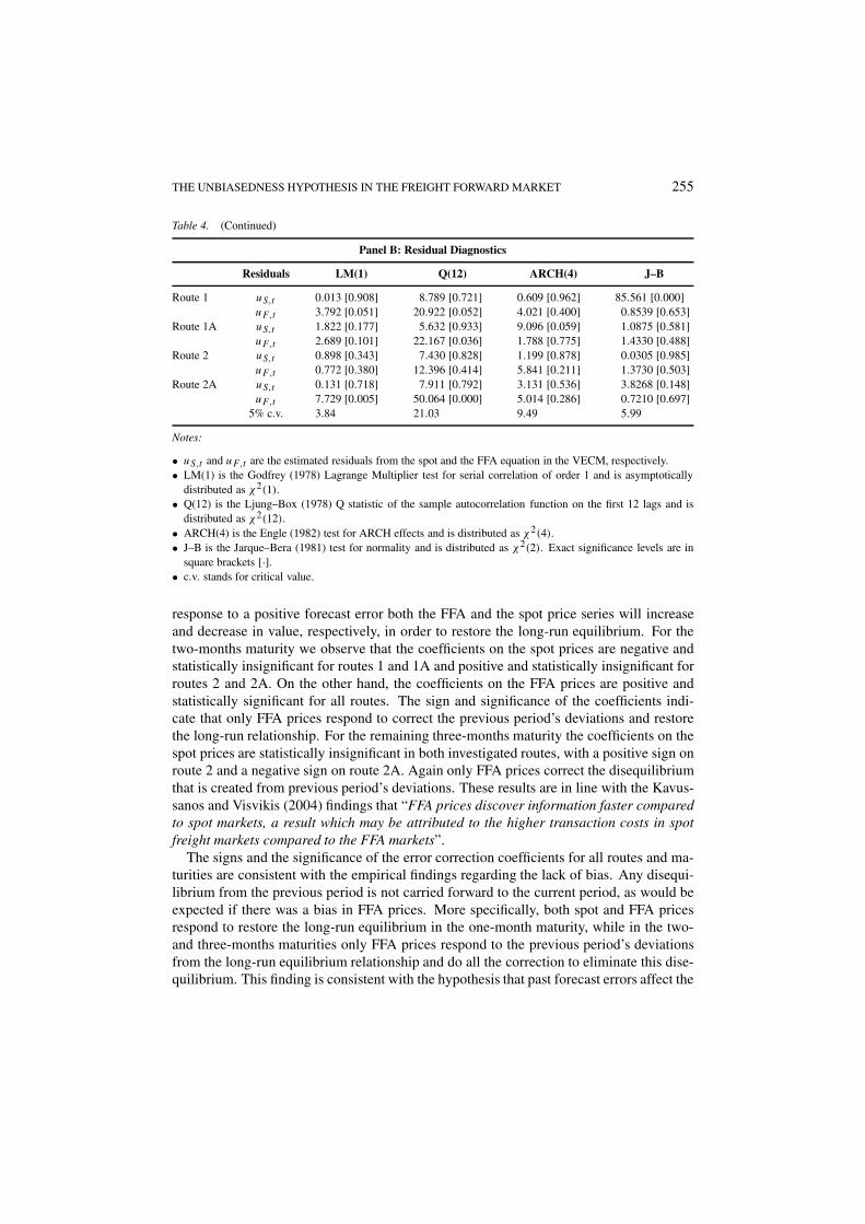
Panel B: Residual Diagnostics
Residuals LM(1) Q(12) ARCH(4) J–B
Route 1 uS,t 0.013 [0.908] 8.789 [0.721] 0.609 [0.962] 85.561 [0.000]uF,t 3.792 [0.051] 20.922 [0.052] 4.021 [0.400] 0.8539 [0.653]
Route 1A uS,t 1.822 [0.177] 5.632 [0.933] 9.096 [0.059] 1.0875 [0.581]uF,t 2.689 [0.101] 22.167 [0.036] 1.788 [0.775] 1.4330 [0.488]
Route 2 uS,t 0.898 [0.343] 7.430 [0.828] 1.199 [0.878] 0.0305 [0.985]uF,t 0.772 [0.380] 12.396 [0.414] 5.841 [0.211] 1.3730 [0.503]
Route 2A uS,t 0.131 [0.718] 7.911 [0.792] 3.131 [0.536] 3.8268 [0.148]uF,t 7.729 [0.005] 50.064 [0.000] 5.014 [0.286] 0.7210 [0.697]
5% c.v. 3.84 21.03 9.49 5.99
Notes:
• uS,t and uF,t are the estimated residuals from the spot and the FFA equation in the VECM, respectively.• LM(1) is the Godfrey (1978) Lagrange Multiplier test for serial correlation of order 1 and is asymptotically
distributed as χ2(1).• Q(12) is the Ljung–Box (1978) Q statistic of the sample autocorrelation function on the first 12 lags and is
distributed as χ2(12).• ARCH(4) is the Engle (1982) test for ARCH effects and is distributed as χ2(4).• J–B is the Jarque–Bera (1981) test for normality and is distributed as χ2(2). Exact significance levels are in
square brackets [·].• c.v. stands for critical value.
response to a positive forecast error both the FFA and the spot price series will increaseand decrease in value, respectively, in order to restore the long-run equilibrium. For thetwo-months maturity we observe that the coefficients on the spot prices are negative andstatistically insignificant for routes 1 and 1A and positive and statistically insignificant forroutes 2 and 2A. On the other hand, the coefficients on the FFA prices are positive andstatistically significant for all routes. The sign and significance of the coefficients indi-cate that only FFA prices respond to correct the previous period’s deviations and restorethe long-run relationship. For the remaining three-months maturity the coefficients on thespot prices are statistically insignificant in both investigated routes, with a positive sign onroute 2 and a negative sign on route 2A. Again only FFA prices correct the disequilibriumthat is created from previous period’s deviations. These results are in line with the Kavus-sanos and Visvikis (2004) findings that “FFA prices discover information faster comparedto spot markets, a result which may be attributed to the higher transaction costs in spotfreight markets compared to the FFA markets”.
The signs and the significance of the error correction coefficients for all routes and ma-turities are consistent with the empirical findings regarding the lack of bias. Any disequi-librium from the previous period is not carried forward to the current period, as would beexpected if there was a bias in FFA prices. More specifically, both spot and FFA pricesrespond to restore the long-run equilibrium in the one-month maturity, while in the two-and three-months maturities only FFA prices respond to the previous period’s deviationsfrom the long-run equilibrium relationship and do all the correction to eliminate this dise-quilibrium. This finding is consistent with the hypothesis that past forecast errors affect the
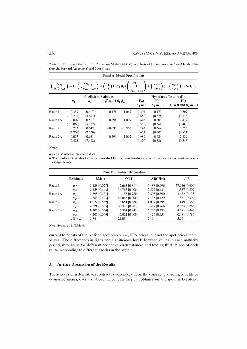
256 KAVUSSANOS, VISVIKIS, AND MENACHOF
Table 5. Estimated Vector Error Correction Model (VECM) and Tests of Unbiasdness for Two-Months FFA(Freight Forward Agreement) and Spot Prices
Panel A: Model Specification
(�St
�Ft,t−1
)= �1
(�St−1
�Ft−1,t−2
)+
(α1α2
)(1 β1 β2)
St−1
1Ft−1,t−2
+
(uS,t
uF,t
);
(uS,t
uF,t
)∼ N(0,�)
Coefficient Estimates Hypothesis Tests on β ′α1 α2 β ′ = ( 1 β1 β2 ) H0: H0: H0:
β1 = 0 β2 = −1 β1 = 0 and β2 = −1
Route 1 −0.359 0.417 1 0.178 −1.067 0.204 0.173 0.507(−0.271) (4.601) [0.652] [0.678] [0.776]
Route 1A −0.009 0.517 1 0.896 −1.097 0.846 0.809 2.434(−0.066) (5.377) [0.358] [0.368] [0.488]
Route 2 0.213 0.642 1 −0.099 −0.965 0.242 0.264 0.395(1.701) (7.209) [0.623] [0.607] [0.821]
Route 2A 0.057 0.631 1 0.591 −1.062 0.989 0.924 2.129(0.423) (7.482) [0.320] [0.336] [0.345]
Notes:
• See also notes in previous tables.• The results indicate that for the two-months FFA prices unbiasedness cannot be rejected at conventional levels
of significance.
Panel B: Residual Diagnostics
Residuals LM(1) Q(12) ARCH(4) J–B
Route 1 uS,t 3.128 [0.077] 7.663 [0.811] 0.188 [0.996] 57.946 [0.000]uF,t 2.158 [0.142] 36.767 [0.000] 2.577 [0.631] 1.357 [0.507]
Route 1A uS,t 2.695 [0.101] 4.157 [0.980] 2.808 [0.590] 3.482 [0.175]uF,t 2.383 [0.123] 44.042 [0.000] 7.135 [0.129] 1.861 [0.394]
Route 2 uS,t 0.027 [0.869] 6.654 [0.880] 1.097 [0.895] 1.149 [0.563]uF,t 4.521 [0.033] 33.336 [0.001] 3.577 [0.466] 0.535 [0.765]
Route 2A uS,t 0.206 [0.650] 5.364 [0.945] 6.226 [0.183] 4.781 [0.092]uF,t 4.206 [0.040] 45.022 [0.000] 4.426 [0.351] 0.481 [0.786]
5% c.v. 3.84 21.03 9.49 5.99
Note: See notes in Table 4.
current forecasts of the realised spot prices, i.e., FFA prices, but not the spot prices them-selves. The differences in signs and significance levels between routes in each maturityperiod, may lie in the different economic circumstances and trading fluctuations of eachroute, responding to different shocks in the system.
5. Further Discussion of the Results
The success of a derivatives contract is dependent upon the contract providing benefits toeconomic agents, over and above the benefits they can obtain from the spot market alone.
THE UNBIASEDNESS HYPOTHESIS IN THE FREIGHT FORWARD MARKET 257
Table 6. Estimated Vector Error Correction Model (VECM) and Tests of Unbiasdness for Three-Months FFA(Freight Forward Agreement) and Spot Prices
Panel A: Model Specification
(�St
�Ft,t−1
)=
(α1α2
)( 1 β1 β2 )
St−1
1Ft−1,t−2
+
(uS,t
uF,t
);
(uS,t
uF,t
)∼ N(0, �)
Coefficient Estimates Hypothesis Tests on β ′α1 α2 β ′ = (1 β1 β2) H0: H0: H0:
β1 = 0 β2 = −1 β1 = 0 and β2 = −1
Route 1 – – – – – – – –Route 1A – – – – – – – –Route 2 0.005 0.314 1 −0.399 −0.863 1.017 1.079 1.346
(0.068) (5.724) [0.313] [0.299] [0.510]Route 2A −0.088 0.287 1 −0.004 −0.997 0.0001 0.0005 0.456
(−0.978) (5.287) [0.998] [0.982] [0.796]
Notes:
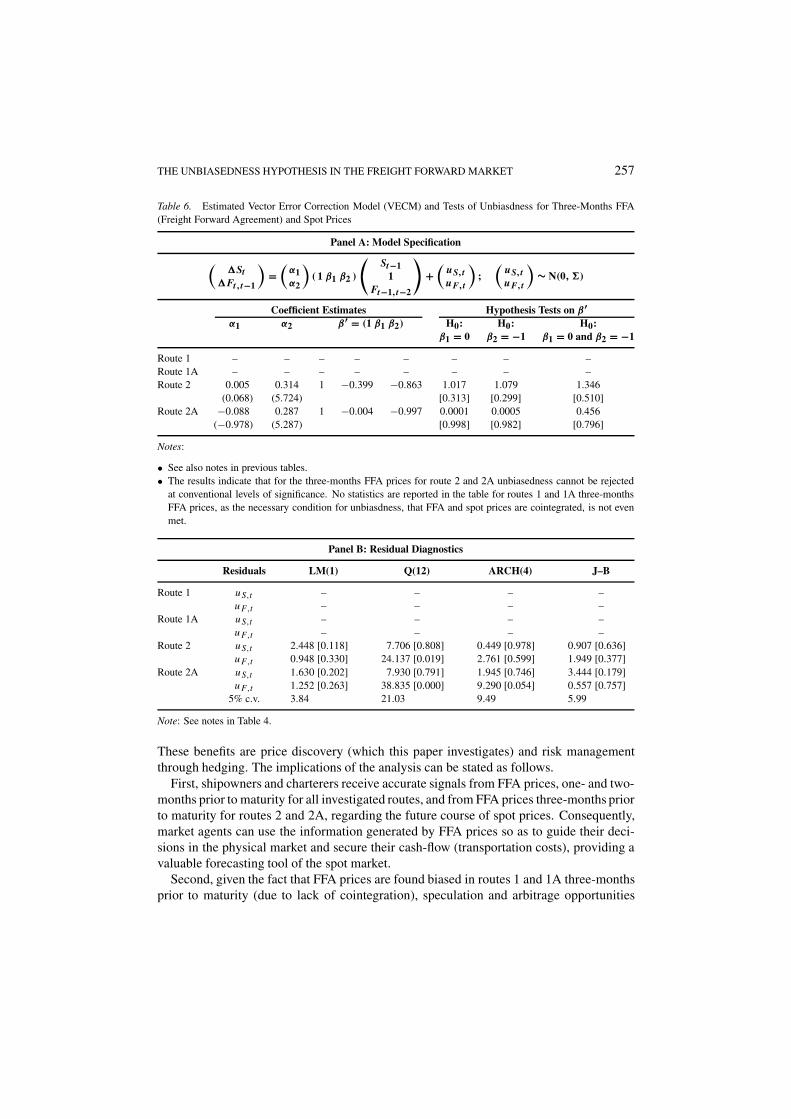
• See also notes in previous tables.• The results indicate that for the three-months FFA prices for route 2 and 2A unbiasedness cannot be rejected
at conventional levels of significance. No statistics are reported in the table for routes 1 and 1A three-monthsFFA prices, as the necessary condition for unbiasdness, that FFA and spot prices are cointegrated, is not evenmet.
Panel B: Residual Diagnostics
Residuals LM(1) Q(12) ARCH(4) J–B
Route 1 uS,t – – – –uF,t – – – –
Route 1A uS,t – – – –uF,t – – – –
Route 2 uS,t 2.448 [0.118] 7.706 [0.808] 0.449 [0.978] 0.907 [0.636]uF,t 0.948 [0.330] 24.137 [0.019] 2.761 [0.599] 1.949 [0.377]
Route 2A uS,t 1.630 [0.202] 7.930 [0.791] 1.945 [0.746] 3.444 [0.179]uF,t 1.252 [0.263] 38.835 [0.000] 9.290 [0.054] 0.557 [0.757]
5% c.v. 3.84 21.03 9.49 5.99
Note: See notes in Table 4.
These benefits are price discovery (which this paper investigates) and risk managementthrough hedging. The implications of the analysis can be stated as follows.
First, shipowners and charterers receive accurate signals from FFA prices, one- and two-months prior to maturity for all investigated routes, and from FFA prices three-months priorto maturity for routes 2 and 2A, regarding the future course of spot prices. Consequently,market agents can use the information generated by FFA prices so as to guide their deci-sions in the physical market and secure their cash-flow (transportation costs), providing avaluable forecasting tool of the spot market.
Second, given the fact that FFA prices are found biased in routes 1 and 1A three-monthsprior to maturity (due to lack of cointegration), speculation and arbitrage opportunities
258 KAVUSSANOS, VISVIKIS, AND MENACHOF
Table 7. Phillips–Hansen (1990) Fully Modified Least Squares Estimates and Tests of Unbiasedness for One,Two and Three Months FFAs (Freight Forward Agreements)
Panel A: One-Month Maturity
Cointegration Tests Coefficient Estimates Hypothesis Testsτ (lags) (a) Z (lags) (b) β1 β2 H0: H0: H0:
β1 = 0 β2 = 1 β1 = 0, β2 = 1
Route 1 −5.852 (0) −6.174 (10) 0.351 0.855 2.136 2.215 2.297(0.240) (0.098) [0.144] [0.137] [0.317]
Route 1A −5.421 (0) −5.362 (10) 0.511 0.942 0.448 0.474 0.923(0.7635) (0.084) [0.503] [0.491] [0.630]
Route 2 −5.919 (0) −6.234 (10) 0.531 0.823 11.234 11.433 11.513(0.158) (0.052) [0.001] [0.001] [0.003]
Route 2A −6.031 (0) −6.117 (10) 0.826 0.908 2.178 2.296 3.625(0.559) (0.061) [0.140] [0.130] [0.163]
Panel B: Two-Months Maturity
Cointegration Tests Coefficient Estimates Hypothesis Testsτ (lags) (a) Z (lags) (b) β1 β2 H0: H0: H0:
β1 = 0 β2 = 1 β1 = 0, β2 = 1
Route 1 −3.909 (0) −3.996 (10) 0.424 0.821 1.889 1.964 2.057(0.316) (0.128) [0.169] [0.161] [0.358]
Route 1A −3.563 (0) −3.493 (10) 1.019 0.885 1.068 1.109 1.556(0.987) (0.109) [0.301] [0.292] [0.459]
Route 2 −3.536 (0) −3.557 (10) 0.621 0.791 6.865 7.088 7.341(0.237) (0.078) [0.009] [0.008] [0.025]
Route 2A −3.932 (0) −3.826 (10) 0.973 0.891 1.428 1.516 2.677(0.814) (0.088) [0.232] [0.218] [0.262]
may create possibilities for excess profits to be made. This, however, could well providean extra incentive for speculators to enter the market and consequently, attract the much-needed volume.
Third, for the 1 and 1A shipping routes three-months prior to maturity, where FFA pricesare found biased, risk-averse agents, with the choice of employing information from theFFA market to construct rolling-hedges, should avoid using these FFA contracts. It appearsthat the specific time of the expiration of the contracts is not a time when the markets areefficient and hence, it is not the time when the hedges should be rolled over. Shipbrokersmust have realised the aforementioned bias and as a policy action they have withdrawnFFA trading for these routes. The results of a clear absence of any cointegration rela-tionship between spot and FFA prices three-months prior to maturity for routes 1 and 1A,confirms prior work of Leuthold (1979) and Naik and Leuthold (1988), which suggest thatthe greater the distance over time the greater the degree of independence between spot andforward prices.
A few words are in order for the finding of no cointegration in routes 1 and 1A for thethree-month contracts. First, lack of cointegration is normally interpreted to imply eithermarket inefficiency or that the markets do not represent the same asset (Engel, 1996). Sec-ond, many shipbrokers suggest that for a creditworthy agent to initiate a FFA contract with
THE UNBIASEDNESS HYPOTHESIS IN THE FREIGHT FORWARD MARKET 259
Table 7. (Continued)
Panel C: Three-Months Maturity
Cointegration Tests Coefficient Estimates Hypothesis Testsτ (lags) (a) Z (lags) (b) β1 β2 H0: H0: H0:
β1 = 0 β2 = 1 β1 = 0, β2 = 1
Route 1 −3.435 (0) −3.448 (10) – – – – –Route 1A −2.984 (0) −3.023 (10) – – – – –Route 2 −3.051 (0) −3.171 (10) – – – – –Route 2A −3.440 (0) −3.434 (10) – – – – –
Notes:
• See also notes in previous tables.• The estimation method to test for unbiasedness is the Phillips and Hansen (1990) Fully-Modified OLS (Or-
dinary Least Squares). Estimation is carried out using Parzen weights; the truncation lag is set equal to 1, 2,and 1 for the one-, two- and three-months maturities, respectively, minimising the SBIC.
• The fully modified estimator [β̃+1 β̃+
2 ]′ is given as [β̃+1 β̃+
2 ]′ = (X′X)−1[X′Y+ − e1k�̃+21], where, X is a
vector of FFA prices ([1, Ft ]t=1,...,T ), Y+ is a vector of realised spot prices ([S+t+1]t=1,...,T ), T is the number
of observations, �̃21 is an estimate of the second-order bias effect of estimating the cointegrating relationshipby OLS, and e1 is assumed to be strictly stationary and ergodic with zero mean and finite covariance.
• (a) τ is the Dickey and Fuller (1981) residual-based test for the null of no-cointegration; the lag length (inparentheses (·)) is determined by minimising the SBIC.
• (b) Z is the Phillips and Perron (1988) test for null of no-cointegration; the truncation lag (in parentheses (·))is computed using the formula suggested by Schwert (1989), i.e., int[12(T /100)0.25].
• The critical values for the τ and Z tests for the null hypothesis of no cointegration (I (1)) are: for the one-month−3.45128, −3.45128, −3.44325 and −3.44325 for routes 1, 1A, 2, and 2A, respectively. For the two-months−3.45348, −3.45348, −3.44515 and −3.44515 for routes 1, 1A, 2, and 2A, respectively. For the three-months−3.45577, −3.45577, −3.44712 and −3.44712 for routes 1, 1A, 2 and 2A, respectively (MacKinnon, 1991).
• The asymptotic standard errors of the coefficient estimates are in parentheses (·). Hypotheses tests on thecoefficient estimates are carried out using a Wald test distributed as χ2 with degrees of freedom equal to thenumber of restrictions. Exact significance levels are in square brackets [·].
• Results for the one- and two-months maturities show that the residuals are stationary, indicating that FFA andrealised spot prices are cointegrated. Moreover, for these maturities, the parameter restrictions of unbiasednesshold for routes 1, 1A, and 2A, but not for route 2. For the three-months maturity, in all routes, none of the FFAand the realised spot prices are cointegrated, and thus, unbiasedness is rejected for all routes.
another, less creditworthy, agent, the former may require a security against a potential de-fault of the latter in the form of a default-premium. Thus, the FFA price in Equation (1)may be substantially different than the spot price, by the existence of such a premium, cre-ating lack of cointegration between them. Another reason for the finding may be that spotand forward prices differ in their ability to incorporate information (1996). The interna-tional dry-bulk spot freight market provides an immediate fixture of a vessel, and suppliersand buyers on the spot market may not have time to respond to new market information.Due to the forward nature of the FFA market, there may be more time for information to beincorporated in prices. Thus, FFA prices, may be able to aggregate more information, andas a result to be set at a different level than spot prices, creating lack of cointegration be-tween them. Yang and Leatham (1999) argue that this difference between commodity spot
260 KAVUSSANOS, VISVIKIS, AND MENACHOF
Table 8. Bierens (1997) Estimates and Tests of Unbiasedness for One, Two and Three Months FFA (FreightForward Agreements)
Panel A: One-Month Maturity
Hypothesis λmin Critical Values Hypothesis gm(r0) Coef. Estimates Hypothesis Testr = 0/r = 1 (r = 1/r = 2) 5% Level r0 = 0, 1, 2 (Spot, FFA) H0: β ′(1 − 1)
Route 1 0.0009 (0.017) 12.99e+003 (1,−0.8446) 1.41a
1.3587 (0.054) 12.16e−00265.44e+001
Route 1A 0.0001 (0.017) 13.54e+004 (1,−0.6126) 2.08a
0.8892 (0.054) 27.23e−00362.80e+000
Route 2 0.0005 (0.017) 12.37e+006 (1,−0.9529) 1.10a
1.3097 (0.054) 15.85e−00591.48e−002
Route 2A 0.0002 (0.017) 18.31e+004 (1,−0.8685) 1.37a
1.5895 (0.054) 72.70e−00461.79e+000
Panel B: Two-Months Maturity
Hypothesis λmin Critical Values Hypothesis gm(r0) Coef. Estimates Hypothesis Testr = 0/r = 1 (r = 1/r = 2) 5% Level r0 = 0, 1, 2 (Spot, FFA) H0: β ′(1 − 1)
Route 1 0.0000 (0.017) 12.21e+007 (1,−0.7914) 1.26a
1.4003 (0.054) 11.73e−00664.61e−003
Route 1A 0.0014 (0.017) 10.14e+002 (1,−0.6122) 3.77a
0.8839 (0.054) 35.45e−00177.79e+002
Route 2 0.0023 (0.017) 16.91e+002 (1,−0.7745) 1.62a
1.4766 (0.054) 88.17e−00262.43e+002
Route 2A 0.0020 (0.017) 29.23e+001 (1,−0.7129) 1.85a
1.9603 (0.054) 28.93e−00136.12e+003
and forward prices may be more significant for commodities traded largely in internationalmarkets. In addition, the argument that transaction costs are lower in the FFA comparedto the spot/physical market contributes to the validity of the argument put forward here(Kavussanos and Visvikis, 2004).
Finally, it may be argued that the low trading volume in routes 1 and 1A in comparisonto the rest of the routes, is exacerbated in the three month FFA contracts when comparedto the one and two month FFA contracts. Shipbrokers provide only actively trading dry-bulk routes as the underlying assets of the FFA contracts. From August 2000 shipbrokersstopped trading FFAs for routes 1 and 1A as their volumes decreased steadily, resultingin FFA bid and offer prices for these routes to be almost unchanged for several months(particularly prices for FFA contracts three-months prior to maturity).23 Consequently,FFA prices may have not followed closely the relevant underlying spot prices, creating adeviation in their long-run relationship.
THE UNBIASEDNESS HYPOTHESIS IN THE FREIGHT FORWARD MARKET 261
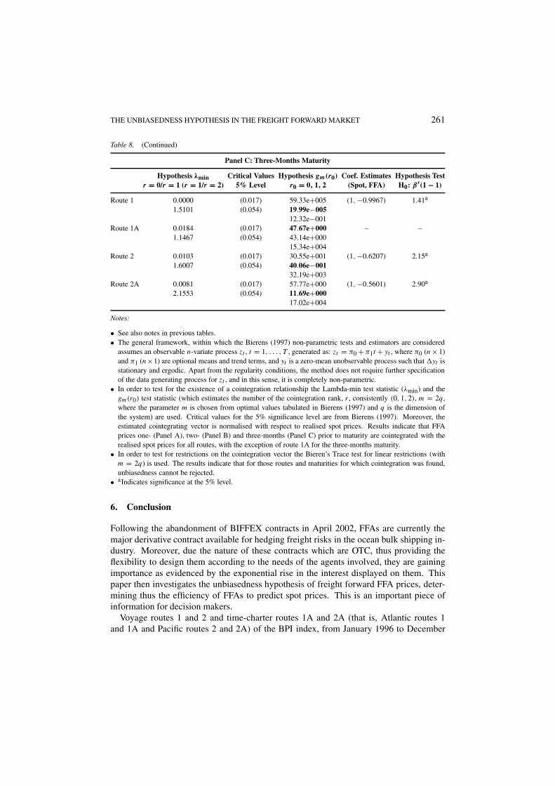
Table 8. (Continued)
Panel C: Three-Months Maturity
Hypothesis λmin Critical Values Hypothesis gm(r0) Coef. Estimates Hypothesis Testr = 0/r = 1 (r = 1/r = 2) 5% Level r0 = 0, 1, 2 (Spot, FFA) H0: β ′(1 − 1)
Route 1 0.0000 (0.017) 59.33e+005 (1,−0.9967) 1.41a
1.5101 (0.054) 19.99e−00512.32e−001
Route 1A 0.0184 (0.017) 47.67e+000 – –1.1467 (0.054) 43.14e+000
15.34e+004Route 2 0.0103 (0.017) 30.55e+001 (1,−0.6207) 2.15a
1.6007 (0.054) 40.06e−00132.19e+003
Route 2A 0.0081 (0.017) 57.77e+000 (1,−0.5601) 2.90a
2.1553 (0.054) 11.69e+00017.02e+004
Notes:
• See also notes in previous tables.• The general framework, within which the Bierens (1997) non-parametric tests and estimators are considered
assumes an observable n-variate process zt , t = 1, . . . , T , generated as: zt = π0 + π1t + yt , where π0 (n× 1)and π1 (n×1) are optional means and trend terms, and yt is a zero-mean unobservable process such that �yt isstationary and ergodic. Apart from the regularity conditions, the method does not require further specificationof the data generating process for zt , and in this sense, it is completely non-parametric.
• In order to test for the existence of a cointegration relationship the Lambda-min test statistic (λmin) and thegm(r0) test statistic (which estimates the number of the cointegration rank, r , consistently (0, 1, 2), m = 2q,where the parameter m is chosen from optimal values tabulated in Bierens (1997) and q is the dimension ofthe system) are used. Critical values for the 5% significance level are from Bierens (1997). Moreover, theestimated cointegrating vector is normalised with respect to realised spot prices. Results indicate that FFAprices one- (Panel A), two- (Panel B) and three-months (Panel C) prior to maturity are cointegrated with therealised spot prices for all routes, with the exception of route 1A for the three-months maturity.
• In order to test for restrictions on the cointegration vector the Bieren’s Trace test for linear restrictions (withm = 2q) is used. The results indicate that for those routes and maturities for which cointegration was found,unbiasedness cannot be rejected.
• aIndicates significance at the 5% level.
6. Conclusion
Following the abandonment of BIFFEX contracts in April 2002, FFAs are currently themajor derivative contract available for hedging freight risks in the ocean bulk shipping in-dustry. Moreover, due the nature of these contracts which are OTC, thus providing theflexibility to design them according to the needs of the agents involved, they are gainingimportance as evidenced by the exponential rise in the interest displayed on them. Thispaper then investigates the unbiasedness hypothesis of freight forward FFA prices, deter-mining thus the efficiency of FFAs to predict spot prices. This is an important piece ofinformation for decision makers.
Voyage routes 1 and 2 and time-charter routes 1A and 2A (that is, Atlantic routes 1and 1A and Pacific routes 2 and 2A) of the BPI index, from January 1996 to December
262 KAVUSSANOS, VISVIKIS, AND MENACHOF
2000, have been examined. Parameter restriction tests on the cointegrating relationship be-tween spot and FFA prices indicate that FFA prices one- and two-months prior to maturityare unbiased predictors of the realised spot prices in all investigated routes. The efficiencyof FFA prices in providing unbiased predictions of spot prices three-months prior to matu-rity gives mixed evidence, with routes 2 and 2A being unbiased estimators while routes 1and 1A are biased estimators of the realised spot prices.
Results are in line with the studies by Moore and Cullen (1995) and Barnhart, McNown,and Wallace (1999), which find unbiasedness for the one- and two-months commodity andforeign exchange forward prices, respectively. However, rejection of unbiasedness for thethree-months FFA prices, for routes 1 and 1A, is not in line with the study of Norrbinand Reffett (1996) which provides evidence in favour of unbiasedness in the three-monthforeign exchange forward prices, but is in line with the study of Krehbiel and Adkins(1993) which find three-months commodity forward prices biased estimators of the realisedspot prices. Thus, it seems that unbiasedness depends on the market and type of contractunder investigation. For the investigated routes and maturities for which unbiasednessholds, market agents can use the FFA prices as indicators of the future course of spotprices, in order to guide their physical market decisions.
Acknowledgements
The authors would like to thank Mr. Robin King from Clarkson Securities Ltd. for pro-viding the data on FFA prices, and the participants in the 2nd International Conferenceon Safety of Maritime Transport, June 2001, Greece, and in the 12th Annual Meetingand Conference of International Association of Maritime Economists, November 2002,Panama City, Panama, for their helpful comments on an earlier draft of this paper. Thepaper has also benefited from the constructive comments of the editor and an anonymousreviewer. Naturally, all remaining errors are those of the authors.
Notes
1. As this paper deals with the dry bulk sector of the shipping industry a few explanations are in order. Thereare distinct markets in the dry bulk sector of the shipping industry, distinguished by vessel size, which in turndefine the type of cargo transported as well as the shipping route (loading and destination area) that vesselsare operating in. Three vessel categories are distinguished in ocean tramp shipping. Handysize vessels(around 30,000 deadweight—dwt henceforth; that is, they carry approximately 30,000 tons of cargo), whichare mainly engaged in transportation of grain commodities from North and South America and Australiato Europe and Asia, and minor dry bulk commodities (such as bauxite and alumina, fertilisers, rice andsugar) around the world. Panamax vessels (around 65,000 dwt) are used primarily in coal and grain and tosome extent in iron ore transportation, from North America and Australia to Japan and West Europe. Themajority of the Capesize fleet (around 120,000 dwt) is engaged in transportation of iron ore from SouthAmerica and Australia to Japan, West Europe and North America and to some extent coal from Australia andNorth America to Japan and West Europe. More details on the structure of these markets may be found inKavussanos (1996).
THE UNBIASEDNESS HYPOTHESIS IN THE FREIGHT FORWARD MARKET 263
2. The Baltic Exchange is the world’s leading international shipping market. Two-thirds of all the world’s openmarket bulk cargo movement is at some stage handled by Baltic members. In addition, it is calculated thatabout half of the world’s sale and purchase of vessels is dealt with through firms represented at the Baltic.
3. Freight fixtures (rentals) come in two main types: Voyage charters, which involve the carriage of cargobetween specified ports for a predetermined freight rate; time-charters, under which a shipowner agrees tohire out the vessel to a charterer (a party with cargo to transport) for a specified period of time, providingcrew together with the vessel, voyage costs being paid by the charterer in this case. Both voyage (spot)and time-charter markets are international, perfectly competitive markets, with a large number of vessel andcargo owners competing for cargo.
4. The BIFFEX freight futures contract was available as a hedging instrument to agents (shipowners and char-terers) operating in ocean freight markets between May 1985 and April 2002. It was listed in the LondonInternational Financial Futures and Options Exchange (LIFFE). When it ceased trading, its underlying assetwas the index basket of the seven routes of the Baltic Panamax Index (BPI) shown in Table 1.
5. A full description of these underlying “commodities” appears in the data section of the paper and in Table 1.6. In futures markets, the trader is required to place with the clearing-house an initial margin, which is an
amount of money on a per contract basis and is set at a size to cover the clearing-house against any loseswhich the trader’s new position might incur during the day. Moreover, futures contracts are mark-to-marketat the end of each trading day. That is, the resulting profit or loss is settled on that day. Traders are requiredto post a variation margin in order to cover the extent to which their trading positions show losses. FFAtransactions costs are 1% of the contract price, shared equally between the buyer and the seller.
7. The major FFA brokers are those in the panel of shipbrokers of the Forward Freight Agreements BrokersAssociation (FFABA), created in 1997. They are: Clarksons Securities Ltd., Fearnleys A/S, Howe Robinson& Co Ltd., GNI Ltd., Ifchor S.A., Mallory Jones Lynch Flynn & Associates Inc, Simpson Spence & YoungLtd., Pasternak, Baum & Company Inc. and Yamamizu Shipping Co. Ltd. London has established itself asthe major FFA market. Currently, FFA contracts have as the underlying asset spot freight rates in routes ofthe Baltic Panamax Index (BPI), the Baltic Handymax Index (BHMI), the Baltic Capesize Index (BCI), andthe Baltic International Tanker Index (BITR).
8. When forward prices are well above (below) the expected spot prices, long (short) hedgers are obliged to buy(sell) the forward contracts at a premium (discount) over the price they expect to prevail on expiration.
9. It is assumed that forward prices are unbiased estimators of expected spot prices (no risk premium) andthat expectations in the market are formed rationally, where market participants are fully informed and theirforecasts when forming their predictions have no systematic mistakes.
10. If a stochastic process must be differenced once in order to become stationary, then the series contains one unitroot and is said to be integrated of order one [I (1)]. If St and Ft,t−n are I (1) series, any linear combinationamong these two series will also be I (1). However, there may be a number b such that St − bFt,t−n = εt
is stationary. In this special case the two price series, St and Ft,t−n, are said to be cointegrated of orderCI(1, 1), implying that they cannot drift apart, but return to the long-run equilibrium level.
11. Johansen (1988), proposes the following two statistics to test for the rank of �: the λtrace(r) =−T
∑ni=r+1 ln(1−λ̂i ) and the λmax(r, r+1) = −T ln(1−λ̂r+i ), where λ̂i and λ̂r+i are the estimated eigen-
values obtained from the estimated � matrix, and T is the number of usable observations. The λtrace teststhe null that there are at most r cointegrating vectors, against the alternative that the number of cointegratingvectors is greater than r and the λmax tests the null that the number of cointegrating vectors is r , againstthe alternative of r + 1. Critical values for the λtrace and λmax statistics are provided by Osterwald–Lenum(1992).
12. The following test proposed by Johansen (1991) is employed to test the most appropriate specification:−T [ln(1 − λ̂∗
2) − ln(1 − λ̂2)] distributed as χ2(1), where λ̂∗2 and λ̂2 represent the smallest eigenvalues
of the model that includes an intercept term in the cointegration vector and an intercept term in the short-runmodel, respectively.
13. The fully modified estimator [β̃+1 β̃
+2 ]′ is given as: [β̃+
1 β̃+2 ]′ = (X′X)−1[X′Y+ − e1k�̃
+21], where, X is a
vector of FFA prices ([1, Ft ]t=1,...,T ), Y+ is a vector of realised spot prices ([S+t+1]t=1,...,T ), T is the num-
ber of observations, �̃21 is an estimate of the second-order bias effect of estimating the cointegrating rela-tionship by OLS, and e1 is assumed to be strictly stationary and ergodic with zero mean and finite covariance.
264 KAVUSSANOS, VISVIKIS, AND MENACHOF
14. The general framework, within which the Bierens (1997) non-parametric tests and estimators are consideredassumes an observable n-variate process zt , t = 1, . . . , T , generated as: zt = π0 + π1t + yt , where π0(n × 1) and π1 (n × 1) are optional means and trend terms, and yt is a zero-mean unobservable processsuch that �yt is stationary and ergodic. Apart from the regularity conditions, the method does not requirefurther specification of the data generating process for zt , and in this sense, it is completely non-parametric.In order to test for the existence of a cointegration relationship the Lambda-min test statistic (λmin) and thegm(r0) test statistic (which estimates the number of the cointegration rank, r , consistently (0, 1, 2), m = 2q,where the parameter m is chosen from optimal values tabulated in Bierens (1997) and q is the dimension ofthe system) are used. Critical values for the 5% significance level are from Bierens (1997). Moreover, theestimated cointegrating vector is normalised with respect to realised spot prices. Finally, in order to test forrestrictions on the cointegration vector the Bieren’s Trace test for linear restrictions (with m = 2q) is used.
15. For routes 1 and 2 (voyage routes) the prices are quoted in $/ton, and for routes 1A and 2A (time-charterroutes) the prices are quoted in $/day.
16. The WF is a constant, unique for each route, and reflects the importance of each route to the index. Forexample, the WF for each BPI route is: 11.185 (route 1), 0.027 (route 1A), 7.067 (route 2), 0.015 (route 2A),9.307 (route 3), 0.031 (route 3A), 0.023 (route 4).
17. Using the freight rate of each route on the maturity day for our analysis, rather than the average of the lastfive/seven trading days, did not change our results qualitatively.
18. The test statistic of the Kwiatkowski et al. (1992) test is calculated as: nt = T −2 ∑Tt=1 K2
t /K2(L), whereL is the lag parameter, Kt is the cumulative sum of the residuals (et ) from a regression of the series on aconstant and a linear trend and K2(L) = T −1 ∑T
t=1 e2t + 2T −1 ∑L
K=1(1 − K/(L + 1))∑T
t=K+1 et et−k .
19. The lag length corresponds to an unrestricted VAR in levels: Xt = ∑pi=1 AiXt−i + et . A VAR with p
lags of the dependent variable can be reparameterised in a VECM with p − 1 lags of first differences of thedependent variable plus the levels terms.
20. Reimers (1992) small sample correction consists of using the factor T − kp instead of T in the calculation ofthe λmax and λtrace, where T is the number of observations, k is the number of regressors, and p is the laglength of the VECM.
21. Use of the Phillips and Hansen (1990) test and the Bierens (1997) test is motivated by the overlappingobservations problem, present in the two- and three-months price series, which may affect the Johansen(1988) test (Hansen and Hodrick, 1980).
22. The discrepancy in our results from the Johansen (1988) test may be attributed to the low power of residual-based cointegration tests compared to the Johansen (1988) test. Another reason is the small-sample correctionof Reimers (1992) in the Johansen (1988) test.
23. This information comes from face to face interviews of the authors with shipbrokers.
References
Akaike, H. (1973). “Information Theory and an Extension of the Maximum Likelihood Principle.” In B. Petrovand F. Csake (eds.), 2nd International Symposium on Information Theory, Budapest: Akademiai Kiado.
Barnhart, S.W., R. McNown, and M.S. Wallace. (1999). “Non-Informative Tests of the Unbiased Forward Ex-change Rate,” Journal of Financial and Quantitative Analysis 34(2), 265–291.
Barnhart, S.W. and A.C. Szakmary. (1991). “Testing the Unbiased Forward Rate Hypothesis: Evidence on UnitRoots, Cointegration, and Stochastic Coefficients,” Journal of Financial and Quantitative Analysis 26(2), 245–267.
Bera, A.K. and C.M. Jarque. (1981). “An Efficient Large-Sample Test for Normality of Observations and Regres-sion Residuals,” Working Papers in Econometrics, Vol. 40, Australian National University, Canberra.
Bessembinder, H. and M.L. Lemmon. (2002). “Equilibrium Pricing and Optimal Hedging in Electricity ForwardMarkets,” Journal of Finance 57, 1347–1382.
Bierens, H.J. (1997). “Nonparametric Cointegration Analysis,” Journal of Econometrics 77, 379–404.Brenner, R. and K. Kroner. (1995). “Arbitrage, Cointegration and Testing the Unbiasedness Hypothesis in Finan-
cial Markets,” Journal of Financial and Quantitative Analysis 30, 23–42.
THE UNBIASEDNESS HYPOTHESIS IN THE FREIGHT FORWARD MARKET 265
Calvet, L., M. Gonzalez-Eiras, and P. Sodini. (2004). “Financial Innovation, Market Participation and AssetPrices,” Journal of Financial and Quantitative Analysis 39(3), September.
Chowdhury, A. (1991). “Futures Market Efficiency: Evidence from Cointegration Tests,” Journal of FuturesMarkets 11, 577–589.
Dickey, D. and W. Fuller. (1981). “Likelihood Ratio Statistics for Autoregressive Time Series with a Unit Root,”Econometrica 49, 1057–1072.
Diebold, F.X., J. Gardeazabal, and K. Yilmaz. (1994). “On Cointegration and Exchange Rate Dynamics,” Journalof Finance 49, 727–735.
Engel, C. (1996). “The Forward Discount Anomaly and the Risk Premium: A Survey of Recent Evidence,”Journal of Empirical Finance 3, 123–192.
Engle, R.F. (1982). “Autoregressive Conditional Heteroskedasticity with Estimates of the Variance of UnitedKingdom Inflation,” Econometrica 50, 987–1008.
Engle, R.F. and C.W. Granger. (1987). “Cointegration and Error Correction: Representation, Estimation, andTesting,” Econometrica 55, 251–276.
Evans, M.D.D. and K.K. Lewis. (1995). “Do Long–Term Swings in the Dollar Affect Estimates of the RiskPremia?” Review of Financial Studies 8, 709–742.
Eydeland, A. and H. Geman. (1998). “Pricing Power Derivatives,” Risk 11(October), 71–74.Fama, E.F. (1970). “Efficient Capital Markets: A Review of Theory and Empirical Work,” Journal of Finance 25,
383–417.Geman, H. and O. Vasicek. (2001). “Plugging into Electricity,” Risk 14(August), 93–97.Granger, C.W.J. and P. Newbold. (1974). “Spurious Regressions in Econometrics,” Journal of Econometrics 2,
1045–1066.Hakkio, C.S. and M. Rush. (1989). “Market Efficiency and Cointegration: An Application to the Sterling and
Deutschemark Exchange Rates,” Journal of International Money and Finance 8, 75–88.Hansen, L. and R. Hodrick. (1980). “Forward Exchange Rates as Optimal Predictors of Futures Spot Rates: An
Econometric Analysis,” Journal of Political Economy 88, 829–853.Johansen, S. (1988). “Statistical Analysis of Cointegration Vectors,” Journal of Economic Dynamics and Control
12, 231–254.Johansen, S. (1991). “Estimation and Hypothesis Testing of Cointegration Vectors in Gaussian Vector Autore-
gressive Models,” Econometrica 59, 1551–1580.Johansen, S. and K. Juselius. (1990). “Maximum Likelihood Estimation and Inference on Cointegration—with
Applications to the Demand for Money,” Oxford Bulletin of Economics and Statistics 52, 169–211.Kavussanos, M.G. (1996). “Comparisons of Volatility in the Dry-Cargo Ship Sector: Spot Versus Time-Charters,
and Small Versus Larger Vessels,” Journal of Transport Economics and Policy, January, 67–82.Kavussanos, M.G. (2002). “Business Risk Measurement and Management in the Cargo Carrying Sector of the
Shipping Industry.” In The Handbook of Maritime Economics and Business, Chapter 30. London: Lloyds ofLondon Press, pp. 661–692.
Kavussanos, M.G. and I.D. Visvikis. (2004). “Market Interactions in Returns and Volatilities between Spot andForward Shipping Freight Markets,” Journal of Banking and Finance 28, 2015–2049.
Kolb, R. (2000). Futures, Options & Swaps, 3rd ed. London: UK, Blackwell Business Publishers.Krehbiel, T. and L. Adkins. (1993). “Cointegration Tests of the Unbiased Expectations Hypothesis in Metals
Markets,” Journal of Futures Markets 13(7), 753–763.Kwiatkowski, D.P., C.B. Phillips, P. Schmidt, and Y. Shin. (1992). “Testing the Null Hypothesis of Stationarity
Against the Alternative of a Unit Root: How Sure Are We that Economic Time Series Have a Unit Root?”Journal of Econometrics 54, 159–178.
Lee, C.I., K.C. Gleason, and I. Mathur. (2000). “Efficiency Tests in the French Derivatives Market,” Journal ofBanking and Finance 24, 787–807.
Leuthold, R.M. (1979). “An Analysis of the Futures-Cash Price Basis for Live Beef Cattle,” North Central Journalof Agricultural Economics 1, 47–52.
Luintel, K.B. and K. Paudyal. (1998). “Common Stochastic Trends between Forward and Spot Exchange Rates,”Journal of International Money and Finance 17, 279–297.
266 KAVUSSANOS, VISVIKIS, AND MENACHOF
MacKinlay, C. and K. Ramaswamy. (1988). “Index-Futures Arbitrage and the Behavior of Stock Index FuturesPrices,” Review of Financial Studies 1, 159–172.
MacKinnon, J.G. (1991). “Critical Values for Cointegration Tests.” In R. Engle and C. Granger (eds.), Long-RunEconomic Relationships. Oxford University, pp. 267–276.
Moore M.J. and Cullen. (1995). “Speculative Efficiency on the London Metal Exchange,” The Manchester School63, 235–256.
Naik, G. and R.M. Leuthold. (1988). “Cash and Futures Price Relationships for Non-Storable Commodities: AnEmpirical Analysis Using a General Theory,” Western Journal of Agricultural Economics 13, 327–338.
Norrbin, S.C. and K.L. Reffett. (1996). “Exogeneity and Forward Rate Unbiasedness,” Journal of InternationalMoney and Finance 15(2), 267–274.
Osterwald-Lenum, M. (1992). “A Note with the Quantiles of the Asymptotic Distribution of the ML CointegrationRank Test Statistics,” Oxford Bulletin of Economics and Statistics 54, 461–472.
Phillips, P.C.B. and B. Hansen. (1990). “Statistical Inference in Instrumental Variables Regression with I (1)
Processes,” Review of Economic Studies 57, 99–125.Phillips, P.C.B. and P. Perron. (1988). “Testing for a Unit Root in Time Series Regressions,” Biometrica 75,
335–346.Reimers, H. (1992). “Comparisons of Tests for Multivariate Cointegration,” Statistical Papers 33, 335–359.Samuelson, P.A. (1965). “Proof that Properly Anticipated Prices Fluctuate Randomly,” Industrial Management
Review 6, 41–49.Schwartz, G. (1978). “Estimating the Dimension of a Model,” Annals of Statistics 6, 461–464.Stein, J.L. (1981). “The Simultaneous Determination of Spot and Futures Prices,” American Economic Review
51(5), 1012–1025.Vasicek, O. (1977). “An Equilibrium Characterization of the Term Structure,” Journal of Financial Economics 5,
177–188.Working, H. (1970). “Economic Functions of Futures Markets.” In H. Bakken (ed.), Futures Trading in Live-
Stock—Origins and Concepts. Chicago: Chicago Mercantile Exchange.Yang, J. and D.J. Leatham. (1999). “Price Discovery in Wheat Futures Markets,” Journal of Agricultural and
Applied Economics 31, 359–370.


