Embed Size (px)
Citation preview
The Review of Regional Studies, Vol. 33, No. 2, 2003, pp. 164− 183
Determining Regional Structure Through Cointegration∗
Harvey Cutler Department of Economics, Colorado State University
Fort Collins, Colorado 80523, email: [email protected]
Scott England Department of Economics, California State University – Fresno Fresno, California 93740-8001, email: [email protected]
Stephan Weiler
Center for the Study of Rural America, Federal Reserve Bank of Kansas City Kansas City, MO 64198, email: [email protected]
Abstract Evaluating regional industrial structures remains an inexact process as traditional aggregation schemes often lump superficially similar but behaviorally distinct industries together. We use pairwise cointegration methods to apply econometric criteria to aggregate detailed industries into behaviorally similar sectors. Based on these aggregations, cointegration guides the proper specification of a regional system to analyze the export versus local nature of core sectors. These methodologies are applied to Denver metropolitan data to demonstrate their utility. The findings indicate previous aggregation schemes are statistically inferior to those generated by this paper’s approach. ∗ The authors thank Stephen Davies, two anonymous referees, and the editor for helpful comments. Any remaining errors are the responsibility of the authors. The views are those of the authors and do not necessarily reflect the positions of the Federal Reserve Bank of Kansas City or the Federal Reserve System.
Cutler, England, and Weiler / The Review of Regional Studies, Vol. 33, No. 2, 2003, pp. 164 − 183 165
1. INTRODUCTION
Sufficient data now exists to pursue time-series analysis of regional economies at the same level of rigor as has been the norm in macroeconomics for several years. However, grouping regional data into manageable aggregated sectors remains a problem. At the widely used SMSA and county levels, data for employment and income can be readily obtained for up to 76 two-digit sectors. Yet estimating such a large system can be difficult. Two approaches have thus far been used to deal with this problem. The first aggregates industries into basic and non-basic components, then conducts empirical analyses using the two series. Other researchers have used standard one-digit SIC aggregates to estimate as many as eight sectors in a time series model. Both approaches have significant drawbacks. This paper first reconsiders the aggregation problem and suggests that a more systematic approach is needed when aggregating sectors. Specification of a cointegration system using these constructed sectors is then addressed, as well as the potential problems arising from incorrect system estimates.
Simple aggregations of basic and non-basic industries ignore the likely idiosyncratic responses
and interactions between sectors. Brown, Coulson, and Engle (1992) examined monthly employment data from Philadelphia from 1975-1987 using location quotient estimates to aggregate industries into basic and non-basic groupings. They used cointegration to estimate the basic multipliers but obtained only limited success. Shoesmith (1992) aggregated employment across all sectors into one aggregate and tested for whether state-level employment was cointegrated with national employment levels. We maintain that there is no reason to assume a priori that all the local sectors will respond in the same way to a shock to a basic sector. In addition, there could be variation of responses of different sectors within a state to a national shock.
More recent efforts have implicitly addressed such issues by using more disaggregated
approaches, such as applying the one-digit SIC taxonomy. Carlino, Defina, and Sill (2001) and Chang and Coulson (2001) used such data to examine the relative importance of local and aggregate shocks in regional economic activity. Yet one-digit SIC aggregates are blunt classifications that may in fact not reflect a region’s more complex industrial structure. Furthermore, such groupings have not been rigorously tested to determine whether industry behavior in fact supports such aggregations. As an example, it is not at all clear that the two-digit sectors of finance, insurance, and real estate can legitimately be grouped together in a broader sector called FIRE. The key question is whether employment variations in these three sectors move together; only in such a case would it in fact be statistically justified to aggregate three otherwise unique industries.
While several methods of aggregation have been developed in the regional literature, the
profession needs to explore the statistical implications of applying different aggregation schemes. Hoen (2002) uses a cluster-based analysis to aggregate multiple two-digit SIC industries into a smaller manageable group of sectors. Input-output matrices are used to identify the connection between industries in terms of intermediate purchases. When one industry purchases a large amount of inputs from another, those two industries can hypothetically be grouped together.1 The key issue in such an approach is determining the benchmark for the amount of intermediate purchases at which sectors should be aggregated together. Interestingly, Hoen’s aggregated groups look very 1 Carlino, Defina, and Sill (2001) use relative sizes of input-output coefficients to impose the needed restrictions to identify a structural VAR model.
Cutler, England, and Weiler / The Review of Regional Studies, Vol. 33, No. 2, 2003, pp. 164 − 183 166
different from the standard one-digit SIC aggregates. Harris, Shonkwiler, and Ebai (1999) use confirmatory factor analysis to aggregate industries into basic and non-basic components for five counties in Nevada. This approach essentially uses a signal extraction technique of decomposing observed employment into basic and non-basic groups.
This paper proposes a time-series-based alternative using cointegration techniques to construct
statistically justified aggregated sectors from two-digit industries. Gonzalo (1993) and Ghose (1994) use pairwise cointegration tests to determine whether two or more series have similar common trends and therefore can be aggregated together. When two series are not cointegrated, they conclude that aggregation will lead to biased parameter values and large standard errors. It is our contention that this pre-testing needs to be performed before any aggregation and eventual empirical analysis can take place, precisely to avoid such potential aggregation biases. Since we are examining time-series employment data in our analysis, which are by their nature non-stationary, we believe the pairwise cointegration method is especially relevant since the other aggregation methods are not consistent with our data. Indeed, Hoen (2002) noted that while his input-output method is useful for cross-sectional analysis, the method does not easily generalize over multiple periods. A critical limitation with the confirmatory factor analysis is that such an approach assumes only one basic and one non-basic sector.
Once a statistically appropriate aggregation structure has been developed, the proper
specification of a regional system becomes the next important challenge. Phillips (1991) and Johansen (1992) demonstrate theoretically that excluding important variables in cointegration analysis can lead to an incorrect number of vectors and biased estimates of coefficients.
These problems surfaced in the money demand literature when a number of researchers had difficulty estimating a stable money demand function. Friedman and Kuttner (1992) and Stock and Watson (1993) each had difficulty estimating a stable money demand function that consisted of real money balances, real income, and an interest rate. Baba, Hendry, and Starr (1992) concluded the problem was due to omitted variable bias. When a larger set of variables was included in the money demand function, a stable relationship could be estimated. Cutler, Davies, and Schmidt (1997) demonstrate that when the simple money demand relation is estimated jointly with consumption, investment, and import markets, the money demand relation appears to be stable over a number of sub-periods from 1960-1993. As will be shown, specification has also been a problem in the regional literature.
We investigate aggregation and specification issues by examining annual data for the Denver Metropolitan Area (DMA). The data set consists of 56 two-digit SIC sectors that are first decomposed into basic and non-basic sectors. Using the pairwise cointegration technique, we obtain five local sectors and three basic sectors, which vary considerably from the standard one-digit SIC groupings. A five-vector system is estimated, with the Vector Error Correction Model (VECM) then being used to determine whether the local sectors adjust to clear their respective markets. To better assess the precision and reliability of the model, we also estimate cointegration systems using both one-digit SIC aggregates as well as aggregated basic and non-basic sectors. Neither of the alternative approaches performs well statistically.
Cutler, England, and Weiler / The Review of Regional Studies, Vol. 33, No. 2, 2003, pp. 164 − 183 167
Section 2 presents the pairwise aggregation method, while Section 3 illustrates the specification of a regional system along with empirical results from the DMA example. Section 4 concludes.
2. AGGREGATION OF A REGIONAL SYSTEM
Two distinct steps outline the sequence of the aggregation process. First, disaggregated industries are divided into basic and non-basic categories. Second, pairwise cointegration tests are used to aggregate each of the industries within the basic and non-basic categories into a manageable number of sectors. After a final aggregation is achieved, Section 3 specifies, estimates, and analyzes a system of multiple cointegrated vectors based on this sectoral structure.
2.1 Determining the Basic and Non-Basic Sectors
Our analysis applies the proposed cointegration-based techniques to the Denver Metropolitan Area (DMA) consisting of Adams, Arapahoe, Denver, Douglas, and Jefferson counties. The state demographer provided annual employment data for 1969-1998 on 56 industries corresponding roughly to the two-digit SIC level.2 Table 1 presents the original 56 industries provided by the Colorado State Demographer's Office. We initially list each industry under its respective one-digit SIC sector.
The first objective is to categorize each industry as predominantly basic or non-basic. As
discussed above, one can use a range of techniques, including location quotient estimates and confirmatory factor analysis, to decompose a group of industries into basic and non-basic groups.3 Nichols and Mushinski (2003) recently developed another technique by using the distribution of regional employment shares to determine the export or local nature of industries. For our case, the State Demographer’s Office conducted an exhaustive survey of Denver industries to determine their basic versus non-basic orientation.4 The State Demographer’s Office combined both survey and nonsurvey (e.g., location quotient) techniques to divide the 56 industries into basic and non-basic groups. The results seemingly provide affirmation for the SIC aggregation as basic and non-basic industries clustered within the broader traditional one-digit sectors. The industries determined to be basic are those within manufacturing, mining, wholesale, and government while the remaining sectors house non-basic “local” industries.
2.2 Aggregating Regional Time Series Through Pairwise Cointegration Tests
This section’s two objectives are to argue for the value of the pairwise cointegration technique as a tool for grouping time series data and then apply the method to aggregate Denver industries into statistically sound sectors.
2 While the standard source for such data is the BEA’s Regional Economic Information Systems (REIS) website (www.bea.doc.gov/bea/regional/reis), it is not possible to obtain all 56 sectors as the data are only at the one digit SIC level. If one is interested in obtaining the disaggregated data for counties in other states, it will be necessary to contact the Demographer’s office or the Department of Labor for that state. We would like to thank Jim Westkott, the state demographer, and Cindy DeGroen for their help in obtaining the disaggregated data, for which confidentiality agreements needed to be signed. 3 See Isserman (1980) for a survey of methods. 4 This survey was part of a larger study performed by the Demographers Office as they attempted to understand the role of export industries in determining Colorado’s economic structure and activity.

Cutler, England, and Weiler / The Review of Regional Studies, Vol. 33, No. 2, 2003, pp. 164 − 183 168
TABLE 1 List of the 56 Sectors in SIC One-Digit Categories
SERVICES MINING TCU Agricultural Services Metal Railroad Transportation Personal Services Coal Local & Suburban Transit Auto Repair & Pkg., Repair Services Oil and Gas Extraction Motor Freight Trans. & Warehousing Amusement & Recreation Services Non-Metallic Minerals Transportation by Air Private Households, & Misc. Services
Transportation Services
Hotels & Other Lodging Places MANUFACTURING Communications Business Services Food & Kindred Products Electric, Gas & Sanitary Health Services Textile Mill Products & Apparel Legal Services Lumber & Wood Prod. incl. Furniture RETAIL Private Education Services Paper & Allied Products Building Material, Hardware, Garden Social Services Printing & Publishing Furniture, Apparel, General Merch. Membership Organizations Chemicals, Plastics, Drugs, Cleaning Agents Food Stores Engineering & Management Services Petroleum Refining, Asphalt, & Roofing Automotive Dealers & Service Stations Rubber, Plastics, and Leather Eating & Drinking Places FIRE Stone, Clay, & Glass Products Miscellaneous Retail Trade Real Estate Primary and Fabricated Metals Finance Industrial, Commercial or Electrical
Machinery WHOLESALE Insurance Transportation Equipment Wholesale Trade Instruments, including Photography CONSTRUCTION Miscellaneous: Jewelry, Toys, Musical GOVERNMENT Building Construction Federal – Civilian Maintenance Federal – Military Heavy Construction State Local
2.2.1 General Approach
The work of Gonzalo (1993) and Ghose (1994) can be used as a template for a practical aggregation methodology. Using Monte Carlo analysis, Ghose investigates the conditions under which two or more series can be aggregated into one composite series. Ghose concludes that if a pair of I(1) variables are cointegrated, then they may be aggregated into one series. However, when two series are not cointegrated, then aggregation will lead to biased parameter values and large standard errors. In the case of more than two series, ensuring that at least significant subsets of aggregated series are cointegrated is thus a desirable objective.
An example provides useful intuition.5 Take xt = (yt zt), a vector containing two non-stationary variables. The equations for both yt and zt are as follows:
(1) yt = µyt + ε yt
(2) zt = µzt + εzt
where µit is a random walk (or the trend component for variable i in time t) and εit is the stationary component of variable i in time t. Thus, yt and zt are cointegrated if (β1yt + β2zt) equals a stationary
5 The following presentation is taken from Enders (1995).
Cutler, England, and Weiler / The Review of Regional Studies, Vol. 33, No. 2, 2003, pp. 164 − 183 169
series. Once these two parameters are applied, then the random walk components for yt and zt will offset one another, yielding only the stationary components, εit. This implies that
(3) β1µyt + β2µzt = 0.
This situation will hold for all t if and only if
(4) µyt = -β2µzt/β1.
Since the common trends for yt and zt are linear combinations of one another, there is only one unique non-stationary process that makes both variables non-stationary. Given that yt and zt both have the same common trend, summing these two series preserves the unique non-stationary characteristics of each series.6
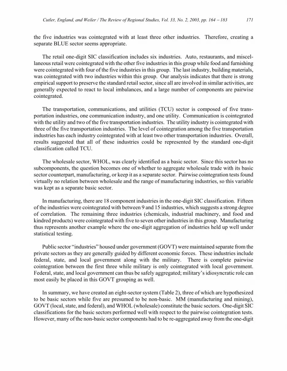
2.2.2 Aggregating Denver Industries
Since our 56 industries have already been divided into two categories, 22 in basic and 34 in non-basic, the process of using the pairwise cointegration approach is simplified. First, the 34 local industries underwent cointegration tests for all combinations. We used the trace and maximum eigenvalue tests to determine whether the sectors are pairwise cointegrated.7 We then repeated the exercise for the 22 basic sectors. It is not likely that we can develop an aggregated scheme where all the industries within a given sector are pairwise cointegrated, but at least a substantial subset of the sectoral components should share this property to minimize potential aggregation biases. We used the one-digit groupings as initial reference points, but in many cases had to explore alternative groupings.
We first consider the construction sector, which consists of building and heavy construction
along with maintenance. Trace tests indicate that heavy construction is cointegrated separately with maintenance and building construction, and maintenance is cointegrated with heavy construction. Overall, it seems appropriate from a statistical perspective to aggregate these three industries into a single sector.
In the FIRE grouping, finance and real estate are not cointegrated with insurance, which raises doubt about this standard one-digit sector. Interestingly, the more recent NAICS classification scheme also splits real estate from its traditional placement in FIRE. We found, however, that finance is cointegrated with real estate, and both of these series are cointegrated with each of the three construction series. Given that real estate services are largely based on the fortunes of construction, combining real estate with the already-evaluated construction industries is plausible theoretically as well as statistically. Finance is also related to the construction sector, given the sizeable role of mortgages and commercial property loans within finance. Our conclusion is to aggregate the three construction series, finance, and real estate into one sector referred to as CRF. 6 Jung, Krutilla, and Boyd (1997) concluded that the four stumpage prices were not pairwise cointegrated, which indicated that individual prices should be used and not a composite price index. Martin-Alvarez, Cano-Fernandez, and Caceres-Hernandez (1999) concluded that a Spanish farm composite price index was not appropriate since all the subcomponents were not pairwise cointegrated. 7 While we do not report all the results of the eigenvalue tests since there are numerous tests, our general objective is to evaluate whether two series were cointegrated at least at the 10 percent significance level. Lag lengths were also explored; in general, results were consistent over multiple lag lengths.

Cutler, England, and Weiler / The Review of Regional Studies, Vol. 33, No. 2, 2003, pp. 164 − 183 170
TABLE 2 Components of the Eight Aggregated Sectors
BLUE MM TCU Agricultural Services Metal Railroad Transportation Personal Services Coal Local & Suburban Transit Auto Repair & Pkg., Repair Services Oil and Gas Extraction Motor Freight Trans. & Warehousing Amusement & Recreation Services Non-Metallic Minerals Transportation by Air Private Households, & Misc. Services Food & Kindred Products Transportation Services Textile Mill Products & Apparel Communications WHITE Lumber & Wood Prod. incl. Furniture Electric, Gas & Sanitary Hotels & Other Lodging Places Paper & Allied Products Business Services Printing & Publishing RET Health Services Chemicals, Plastics, Drugs, Cleaning Agents Building Material, Hardware, Garden Legal Services Petroleum Refining, Asphalt, & Roofing Furniture, Apparel, General Merchandise. Private Education Services Rubber, Plastics, and Leather Food Stores Social Services Stone, Clay, & Glass Products Automotive Dealers & Service Stations Membership Organizations Primary and Fabricated Metals Eating & Drinking Places Engineering & Management Services Industrial, Commercial or Electrical Machinery Miscellaneous Retail Trade Insurance Transportation Equipment Instruments, including Photography GOVT CRF Miscellaneous: Jewelry, Toys, Musical Federal - Civilian Building Construction Federal - Military Maintenance WHOL State Heavy Construction Wholesale Trade Local Finance Real Estate
This newly aggregated sector appears in Table 2, which effectively summarizes the results of the pairwise exercise.
Insurance, the remaining industry, is not cointegrated with building construction, maintenance, or finance, although it is cointegrated with heavy construction, indicating that insurance does not belong with CRF. In contrast, given the service orientation of the insurance industry, it seems possible that insurance would be cointegrated with components of the service sector.
The service sector is likely to be particularly susceptible to aggregation biases when analyzed at
its traditional one-digit summary level, given the diversity of its component industries. For that reason, services are a principal focus in this industry triage process. One of the major NAICS revisions was in fact to split the formerly monolithic service sector into seven more cohesive units. We performed pairwise cointegration tests on all combinations of industries in the service sector. Our tests resulted in dividing services into two groups that can generally be referred to as blue-collar and white-collar, since, legal and medical services are likely to follow different employment patterns than amusement services.
In terms of the white-collar (WHITE) sector, business services, legal, and membership services are cointegrated with all of the other industries within WHITE. Health, private education, membership, and engineering services are cointegrated with at least three other industries. These findings indicate that these seven industries could be aggregated into one sector called WHITE. The insurance industry is also cointegrated with four of the white-collar services, so insurance is integrated into WHITE. Aggregating blue-collar industries was slightly less successful, but each of
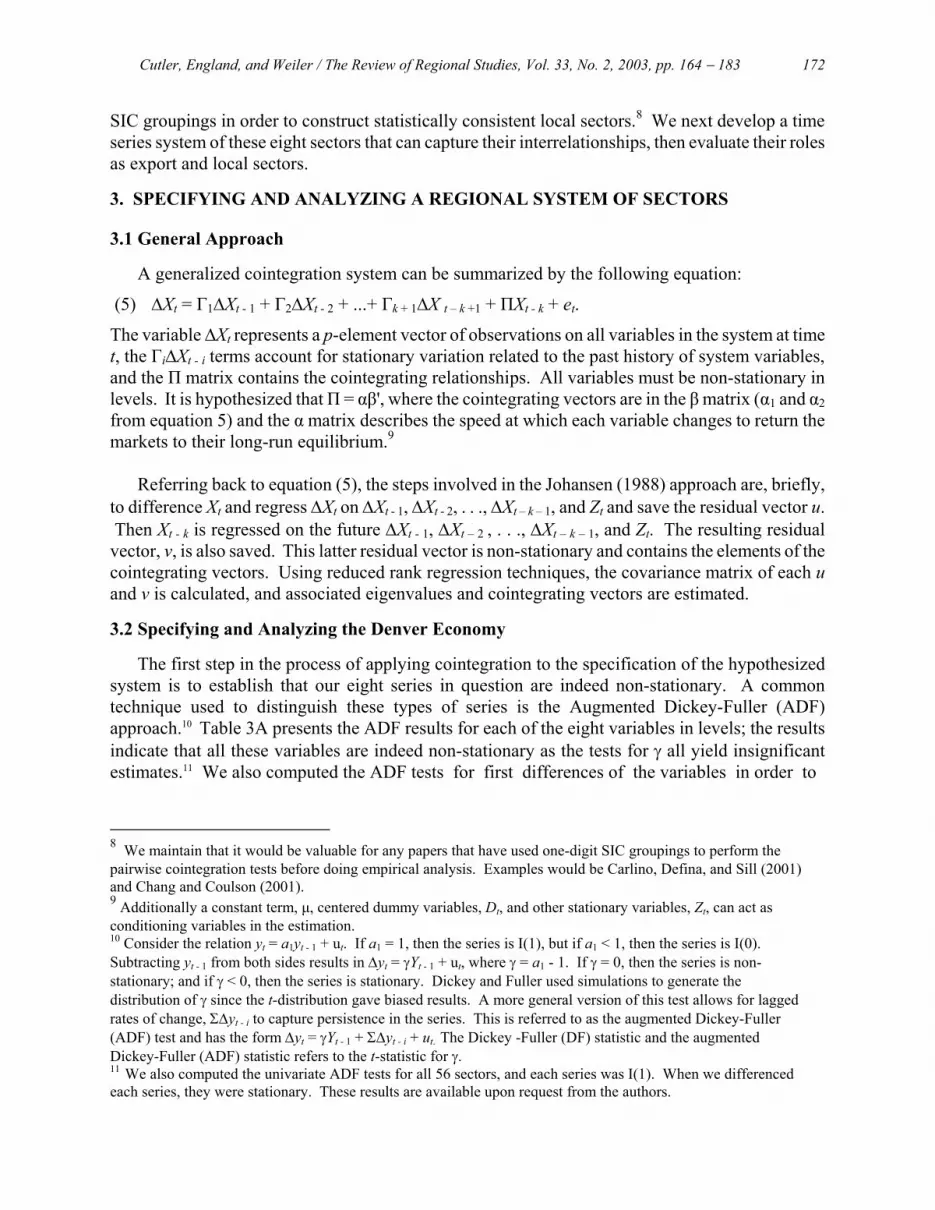
Cutler, England, and Weiler / The Review of Regional Studies, Vol. 33, No. 2, 2003, pp. 164 − 183 171
the five industries was cointegrated with at least three other industries. Therefore, creating a separate BLUE sector seems appropriate.
The retail one-digit SIC classification includes six industries. Auto, restaurants, and miscel-
laneous retail were cointegrated with the other five industries in this group while food and furnishing were cointegrated with four of the five industries in this group. The last industry, building materials, was cointegrated with two industries within this group. Our analysis indicates that there is strong empirical support to preserve the standard retail sector, since all are involved in similar activities, are generally expected to react to local imbalances, and a large number of components are pairwise cointegrated.
The transportation, communications, and utilities (TCU) sector is composed of five trans-
portation industries, one communication industry, and one utility. Communication is cointegrated with the utility and two of the five transportation industries. The utility industry is cointegrated with three of the five transportation industries. The level of cointegration among the five transportation industries has each industry cointegrated with at least two other transportation industries. Overall, results suggested that all of these industries could be represented by the standard one-digit classification called TCU.
The wholesale sector, WHOL, was clearly identified as a basic sector. Since this sector has no
subcomponents, the question becomes one of whether to aggregate wholesale trade with its basic sector counterpart, manufacturing, or keep it as a separate sector. Pairwise cointegration tests found virtually no relation between wholesale and the range of manufacturing industries, so this variable was kept as a separate basic sector.
In manufacturing, there are 18 component industries in the one-digit SIC classification. Fifteen
of the industries were cointegrated with between 9 and 15 industries, which suggests a strong degree of correlation. The remaining three industries (chemicals, industrial machinery, and food and kindred products) were cointegrated with five to seven other industries in this group. Manufacturing thus represents another example where the one-digit aggregation of industries held up well under statistical testing.
Public sector “industries” housed under government (GOVT) were maintained separate from the
private sectors as they are generally guided by different economic forces. These industries include federal, state, and local government along with the military. There is complete pairwise cointegration between the first three while military is only cointegrated with local government. Federal, state, and local government can thus be safely aggregated; military’s idiosyncratic role can most easily be placed in this GOVT grouping as well.
In summary, we have created an eight-sector system (Table 2), three of which are hypothesized to be basic sectors while five are presumed to be non-basic. MM (manufacturing and mining), GOVT (local, state, and federal), and WHOL (wholesale) constitute the basic sectors. One-digit SIC classifications for the basic sectors performed well with respect to the pairwise cointegration tests. However, many of the non-basic sector components had to be re-aggregated away from the one-digit
Cutler, England, and Weiler / The Review of Regional Studies, Vol. 33, No. 2, 2003, pp. 164 − 183 172
SIC groupings in order to construct statistically consistent local sectors.8 We next develop a time series system of these eight sectors that can capture their interrelationships, then evaluate their roles as export and local sectors.
3. SPECIFYING AND ANALYZING A REGIONAL SYSTEM OF SECTORS
3.1 General Approach
A generalized cointegration system can be summarized by the following equation:
(5) ∆Xt = Γ1∆Xt - 1 + Γ2∆Xt - 2 + ...+ Γk + 1∆X t – k +1 + ΠXt - k + et.
The variable ∆Xt represents a p-element vector of observations on all variables in the system at time t, the Γi∆Xt - i terms account for stationary variation related to the past history of system variables, and the Π matrix contains the cointegrating relationships. All variables must be non-stationary in levels. It is hypothesized that Π = αβ', where the cointegrating vectors are in the β matrix (α1 and α2 from equation 5) and the α matrix describes the speed at which each variable changes to return the markets to their long-run equilibrium.9
Referring back to equation (5), the steps involved in the Johansen (1988) approach are, briefly, to difference Xt and regress ∆Xt on ∆Xt - 1, ∆Xt - 2, . . ., ∆Xt – k – 1, and Zt and save the residual vector u. Then Xt - k is regressed on the future ∆Xt - 1, ∆Xt – 2 , . . ., ∆Xt – k – 1, and Zt. The resulting residual vector, v, is also saved. This latter residual vector is non-stationary and contains the elements of the cointegrating vectors. Using reduced rank regression techniques, the covariance matrix of each u and v is calculated, and associated eigenvalues and cointegrating vectors are estimated.
3.2 Specifying and Analyzing the Denver Economy
The first step in the process of applying cointegration to the specification of the hypothesized system is to establish that our eight series in question are indeed non-stationary. A common technique used to distinguish these types of series is the Augmented Dickey-Fuller (ADF) approach.10 Table 3A presents the ADF results for each of the eight variables in levels; the results indicate that all these variables are indeed non-stationary as the tests for γ all yield insignificant estimates.11 We also computed the ADF tests for first differences of the variables in order to
8 We maintain that it would be valuable for any papers that have used one-digit SIC groupings to perform the pairwise cointegration tests before doing empirical analysis. Examples would be Carlino, Defina, and Sill (2001) and Chang and Coulson (2001). 9 Additionally a constant term, µ, centered dummy variables, Dt, and other stationary variables, Zt, can act as conditioning variables in the estimation. 10 Consider the relation yt = a1yt - 1 + ut. If a1 = 1, then the series is I(1), but if a1 < 1, then the series is I(0). Subtracting yt - 1 from both sides results in ∆yt = γYt - 1 + ut, where γ = a1 - 1. If γ = 0, then the series is non-stationary; and if γ < 0, then the series is stationary. Dickey and Fuller used simulations to generate the distribution of γ since the t-distribution gave biased results. A more general version of this test allows for lagged rates of change, Σ∆yt - i to capture persistence in the series. This is referred to as the augmented Dickey-Fuller (ADF) test and has the form ∆yt = γYt - 1 + Σ∆yt - i + ut. The Dickey -Fuller (DF) statistic and the augmented Dickey-Fuller (ADF) statistic refers to the t-statistic for γ. 11 We also computed the univariate ADF tests for all 56 sectors, and each series was I(1). When we differenced each series, they were stationary. These results are available upon request from the authors.

Cutler, England, and Weiler / The Review of Regional Studies, Vol. 33, No. 2, 2003, pp. 164 − 183 173
TABLE 3A Augmented Dickey-Fuller Tests, in Levels
Variable ADF: Intercept ADF: Intercept & Trend ADF: None BLUE -2.44 -1.93 1.22 WHITE -1.56 -2.88 3.94 RET -1.76 -2.38 3.02 CRF -0.79 -2.07 1.73 TCU -0.35 -1.85 3.96 GOVT -2.13 -2.52 1.67 WHOL -1.16 -1.50 1.81 MM -3.64 -2.58 1.20 Critical Values: Intercept:
1%: -3.70 5%: -2.98 10%: -2.63
Intercept & Trend: 1%: -4.34 5%: -3.59 10%: -3.23
None: 1%: -2.65 5%: -1.95 10%: -1.62
TABLE 3B
Augmented Dickey-Fuller Tests, in First Differences Variable ADF: Intercept ADF: Intercept & Trend ADF: None BLUE -2.87 -2.97 -2.54 WHITE -4.52 -4.83 -1.15 RET -4.19 -4.43 -2.49 CRF -4.09 -3.93 -3.56 TCU -4.64 -4.55 -1.89 GOVT -2.70 -3.28 -2.05 WHOL -3.08 -3.08 -2.38 MM -3.45 -4.65 -3.24 Critical Values: Intercept:
1%: -3.70 5%: -2.98 10%: -2.63
Intercept & Trend: 1%: -4.34 5%: -3.59 10%: -3.23
None: 1%: -2.65 5%: -1.95
10%: -1.62
determine whether the series were truly I(1). These results appear in Table 3B. All tests indicated at least at the ten percent level that the first differences are stationary.
To determine the optimal lag length for the cointegration, we used the Akaike Information Criteria (AIC) test and the Schwarz Bayesian Criterion (SBC), tests that emphasize minimizing the sum of square residuals. Both tests indicated that two lags should be used.
Pairwise cointegration tests produced five non-basic or local sectors in the DMA. While we are interested in how local sectors respond to basic sector evolutions, it is also important to allow for the distinct possibility that each of the local sectors will have a unique relationship with respect to each of the basic sectors. Therefore, our hypothesis is that there should be five cointegrating vectors in the DMA, with each vector representing a local sector’s relationship to the basic sectors.
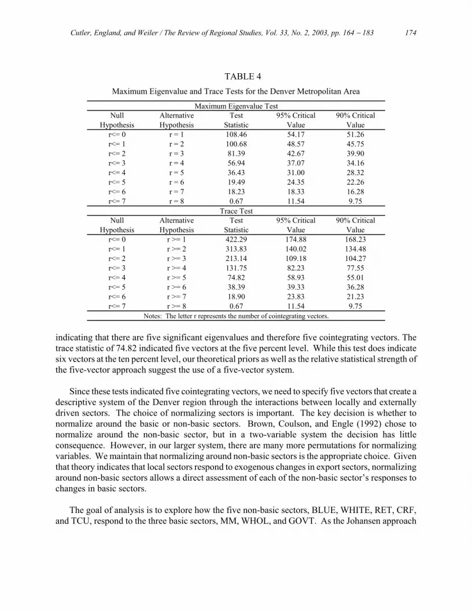
The maximum eigenvalue and trace tests were used to determine the number of cointegrating vectors. These results appear in Table 4. The maximum eigenvalue statistic was 36.43 and significant at the five percent level when testing for four cointegrating vectors versus five vectors,
Cutler, England, and Weiler / The Review of Regional Studies, Vol. 33, No. 2, 2003, pp. 164 − 183 174
TABLE 4 Maximum Eigenvalue and Trace Tests for the Denver Metropolitan Area
indicating that there are five significant eigenvalues and therefore five cointegrating vectors. The trace statistic of 74.82 indicated five vectors at the five percent level. While this test does indicate six vectors at the ten percent level, our theoretical priors as well as the relative statistical strength of the five-vector approach suggest the use of a five-vector system.
Since these tests indicated five cointegrating vectors, we need to specify five vectors that create a descriptive system of the Denver region through the interactions between locally and externally driven sectors. The choice of normalizing sectors is important. The key decision is whether to normalize around the basic or non-basic sectors. Brown, Coulson, and Engle (1992) chose to normalize around the non-basic sector, but in a two-variable system the decision has little consequence. However, in our larger system, there are many more permutations for normalizing variables. We maintain that normalizing around non-basic sectors is the appropriate choice. Given that theory indicates that local sectors respond to exogenous changes in export sectors, normalizing around non-basic sectors allows a direct assessment of each of the non-basic sector’s responses to changes in basic sectors.
The goal of analysis is to explore how the five non-basic sectors, BLUE, WHITE, RET, CRF,
and TCU, respond to the three basic sectors, MM, WHOL, and GOVT. As the Johansen approach
Trace TestNull Alternative Test 95% Critical 90% Critical
Valuer<= 0 r >= 1 422.29 174.88 168.23
Hypothesis Hypothesis Statistic Value
134.48r<= 2 r >= 3 213.14 109.18 104.27r<= 1 r >= 2 313.83 140.02
77.55r<= 4 r >= 5 74.82 58.93 55.01r<= 3 r >= 4 131.75 82.23
36.28r<= 6 r >= 7 18.90 23.83 21.23r<= 5 r >= 6 38.39 39.33
r<= 7 r >= 8 0.67 11.54 9.75Notes: The letter r represents the number of cointegrating vectors.
Maximum Eigenvalue TestNull Alternative Test 95% Critical 90% Critical
Hypothesis Hypothesis Valuer<= 0 r = 1 108.46 54.17 51.26
Statistic Value
45.75r<= 2 r = 3 81.39 42.67 39.90r<= 1 r = 2 100.68 48.57
34.16r<= 4 r = 5 36.43 31.00 28.32r<= 3 r = 4 56.94 37.07
22.26r<= 6 r = 7 18.23 18.33 16.28r<= 5 r = 6 19.49 24.35
9.75r<= 7 r = 8 0.67 11.54
Cutler, England, and Weiler / The Review of Regional Studies, Vol. 33, No. 2, 2003, pp. 164 − 183 175
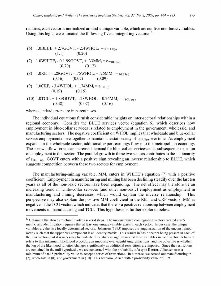
requires, each vector is normalized around a unique variable, which are our five non-basic variables. Using this logic, we estimated the following five cointegrating vectors:12
(6) 1.0BLUEt + 2.7GOVTt - 2.4WHOLt = εBLUE(t) (1.1) (0.20)
(7) 1.0WHITEt - 0.1.99GOVTt + .33MMt = εWHITE(t) (0.70) (0.12)
(8) 1.0RETt - .28GOVTt - .75WHOLt + .26MMt = εRET(t) (0.16) (0.07) (0.09)
(9) 1.0CRFt - 3.4WHOLt + 1.74MMt = εCRF (t) (0.19) (0.15)
(10) 1.0TCUt + 1.89GOVTt - .28WHOLt - 0.76MMt = εTCU (t) , (0.48) (0.07) (0.16)
where standard errors are in parentheses.
The individual equations furnish considerable insights on inter-sectoral relationships within a regional economy. Consider the BLUE services vector (equation 6), which describes how employment in blue-collar services is related to employment in the government, wholesale, and manufacturing sectors. The negative coefficient on WHOL implies that wholesale and blue-collar service employment move together to maintain the stationarity of εBLUE(t) over time. As employment expands in the wholesale sector, additional export earnings flow into the metropolitan economy. These new inflows create an increased demand for blue-collar services and a subsequent expansion of employment in this sector. The parallel growth in these two sectors contributes to the stationarity of εBLUE(t). GOVT enters with a positive sign revealing an inverse relationship to BLUE, which suggests competition between these two sectors for employment.
The manufacturing-mining variable, MM, enters in WHITE’s equation (7) with a positive
coefficient. Employment in manufacturing and mining has been declining steadily over the last ten years as all of the non-basic sectors have been expanding. The net effect may therefore be an increasing trend in white-collar services (and other non-basic) employment as employment in manufacturing and mining decreases, which would explain the inverse relationship. This perspective may also explain the positive MM coefficient in the RET and CRF vectors. MM is negative in the TCU vector, which indicates that there is a positive relationship between employment movements in manufacturing and TCU. This hypothesis is further explored below. 12 Obtaining the above structure involves several steps. The unconstrained cointegrating vectors created a 8×5 matrix, and identification requires that at least one unique variable exists in each vector. In our case, the unique variables are the five locally determined sectors. Johansen (1995) imposes a triangularization of the unconstrained matrix such that the upper 5×5 component is an identity matrix. This results in basic sectors being present in each of the four vectors, but it is necessary to evaluate the statistical significance of these variables in each vector. Johansen refers to this maximum likelihood procedure as imposing over-identifying restrictions, and the objective is whether the log of the likelihood function changes significantly as additional restrictions are imposed. Since the restrictions are contained in the null hypothesis, we are concerned with the probability of a type II error; Johansen uses a minimum of a 0.15 probability value to accept a series of restrictions. In our case, we zeroed out manufacturing in (7), wholesale in (8), and government in (10). This scenario passed with a probability value of 0.19.
Cutler, England, and Weiler / The Review of Regional Studies, Vol. 33, No. 2, 2003, pp. 164 − 183 176
The other four vectors, equations (8) – (10), depict the industrial structure for the remainder of
the Denver metropolitan economy through the RET, CRF, and TCU vectors, respectively. The WHOL variable consistently enters the vectors with a negative sign, which is consistent with wholesale trade’s export orientation. WHOL exists in each vector but WHITE and is negative in all except TCU.
The combination of pairwise aggregation along with the regional system’s specification and
cointegration results can shed considerable light on a regional economy. For example, in the case of Denver, the linkages between the otherwise disparate construction, real estate, and finance industries not only led to their being grouped in a single non-basic sector, but also suggest that the industries surrounding construction in this rapidly growing metropolitan area have achieved an unusually high degree of integration. Such a situation hints at potential efficiencies in the rapid provision of new residential and non-residential development in the area. The fact that non-basic sectors did not follow traditional one-digit SIC categories indicates that internal linkages among local industries are likely to vary across different regions, in part demonstrating different stages of the agglomeration process.
The system specification and analysis provide further insights on the local economy. The
Denver results suggests that government employment expansions tend to promote white-collar services and retail jobs in the area, but may crowd out some blue-collar services and TCU positions. Such a result could be due to public provision of previously privately-provided goods or services (e.g., transit) or public sector competition for overlapping supplies of labor. In this sense, a careful statistical systems analysis can guide researchers and local officials towards productive further inquiries on specific industries and their interrelationships.
3.3 Speeds of Adjustment
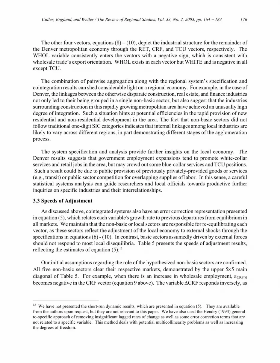
As discussed above, cointegrated systems also have an error correction representation presented in equation (5), which relates each variable's growth rate to previous departures from equilibrium in all markets. We maintain that the non-basic or local sectors are responsible for re-equilibrating each vector, as these sectors reflect the adjustment of the local economy to external shocks through the specifications in equations (6) - (10). In contrast, basic sectors assumedly driven by external forces should not respond to most local disequilibria. Table 5 presents the speeds of adjustment results, reflecting the estimates of equation (5).13
Our initial assumptions regarding the role of the hypothesized non-basic sectors are confirmed. All five non-basic sectors clear their respective markets, demonstrated by the upper 5×5 main diagonal of Table 5. For example, when there is an increase in wholesale employment, εCRF(t) becomes negative in the CRF vector (equation 9 above). The variable ∆CRF responds inversely, as
13 We have not presented the short-run dynamic results, which are presented in equation (5). They are available from the authors upon request, but they are not relevant to this paper. We have also used the Hendry (1993) general-to-specific approach of removing insignificant lagged rates of change as well as some error correction terms that are not related to a specific variable. This method deals with potential multicollinearity problems as well as increasing the degrees of freedom.
Cutler, England, and Weiler / The Review of Regional Studies, Vol. 33, No. 2, 2003, pp. 164 − 183 177
TABLE 5 Speeds of Adjustment Analysis (standard errors in parentheses)
Variable εBLUE(t - 1) εWHITE(t - 1) εRET(t - 1) εCRF(t - 1) εTCU(t - 1)
∆BLUE -1.60*** (0.86)
-2.46 (1.65)
3.07 (1.99)
0.01 (0.59)
1.21 (0.95)
∆WHITE
-0.23**(0.11)
-0.31 (0.45)
0.17 (0.14)
-0.002 (0.18)
∆RET 0.42* (0.16)
0.75* (0.32)
-0.73* (0.33)
-0.10 (0.13)
0.33 (0.20)
∆CRF (0.01) (0.13)
-0.49* (0.12)
0.57*** (0.32)
∆TCU -0.42** (0.21)
-1.43* (0.40)
-0.93** (0.48)
0.47* (0.14)
-1.00* (0.23)
∆GOVT 0.20 (0.17)
0.55 (0.32)
-0.65 (0.38)
0.08 (0.11)
-0.01 (0.18)
∆WHOL -0.12 (0.40)
0.02 (0.76)
-0.01 (0.92)
0.22 (0.27)
0.97** (0.44)
∆MM -0.12 (0.46)
-0.45 (0.89)
0.98 (1.07)
-0.28 (0.32)
0.12 (0.51)
Notes: *** significant at the 10% level ** significant at the 5% level
* significant at the 1% level
indicated by the significant coefficient of -0.49 attached to εCRF(t - 1), and causes an increase in εCRF(t) to offset the initial wholesale-induced shock. Re-equilibration of this market thus occurs through expanding employment in the CRF sector. Similar results are obtained across the other local sectors, BLUE, WHITE, RET, and TCU, as their coefficients along the main diagonal are -1.60, -0.23, -0.73, and -1.00, respectively. All parameters are significant at least at the 10 percent level and indicate that each local sector re-equilibrates their respective vector. Our aggregation scheme appears to have performed well as the hypothesized local sectors all respond to local disequilibria conditions.14
The manufacturing and mining sector, which is assumed to be basic, does not respond at all to
local disequilibria conditions since its estimated coefficients are not statistically distinguishable from zero. As expected, manufacturing employment should be influenced by the external demand patterns based on national and international sales. Therefore, the combination of manufacturing and mining appears to be a good approximation of a basic sector. Similarly, GOVT does not respond to disequilibrium in any of the cointegrating relations either. WHOL responds to disequilibrium with the TCU sector only, indicating that a distinct component of WHOL appears to be involved in local activity. Unfortunately, it is not possible at this stage to dissect this dynamic any further, given current data limitations.
While only having 30 observations is not optimal for time-series analysis, even such relatively
limited data can be leveraged using Johansen’s method, which can effectively mitigate potential degrees of freedom problems. The unconstrained vectors contain 40 parameters, but are quickly reduced to 15 using the techniques described in footnote 12. Further parameter reductions are 14 It is interesting that Harris, Shonkwiler, and Ebai (1999) examine their bivariate cointegration system in a similar manner but do not emphasize the use of the VECM in the way described in our paper.
Cutler, England, and Weiler / The Review of Regional Studies, Vol. 33, No. 2, 2003, pp. 164 − 183 178
obtained by statistically eliminating several of the basic sectors in equations (6) – (10). The fact that the remaining variables are all significant and the results furthermore strongly reflect existing regional theory reinforces confidence in the noted techniques and resultant system.
3.4 Comparing Alternative Aggregation Schemes and Specification Issues
Comparing our results to previous systems analyses in the literature underscores the value of our approach. As discussed above, Brown, Coulson, and Engle (1992) estimated a simplified system of aggregated industries divided into a single non-basic sector and a single basic sector. Nishiyama (1997) uses a similar approach for data from California, Massachusetts, and Texas, conducting cointegration tests for each state. Nishiyama concludes that cointegration generally does not exist in these series and proceeds to estimate the data in first differences. Crane and Nourzad (1998) maintain that this limited success raises doubt about the use of cointegration analysis in the regional area. Using the same approach with our data, the eigenvalue tests for such a two-variable system rejected the presence of the predicted single cointegrating vector. One would therefore have to conclude that there is no long-run stable relationship between basic and non-basic sectors in the Denver economy. Yet our results above clearly indicate that such a conclusion would be incorrect.
We also examined the standard one-digit SIC classifications as the relevant sectors in our multiple vector approach. For example, instead of combining construction with real estate as the pairwise cointegration tests suggested, we specified construction industries in their traditional separate sectoral category. We estimated a variety of systems using such standard one-digit SIC classifications and had difficulty finding significant statistical results. There were problems reconciling the eigenvalue tests with estimating significant coefficients in the cointegrating vectors. These systems were also plagued with a large number of insignificant estimated coefficients. Furthermore, the speeds of adjustment results did not find much support for the local sectors clearing their respective vectors. These experiments support our contention that both proper aggregation and proper system specification are crucial to meaningful regional time-series analysis.
Estimating a multiple vector system with properly aggregated sectors may still not be sufficient
to yield useful results if one does not normalize around the correct variables. Theory implies that normalizing around the local variables is appropriate. If one normalizes around the basic sectors, estimation results will inevitably be affected. Using the latter approach with our data, many more of the cointegrating coefficients were insignificant compared to equations (6) – (10). In fact, it was difficult even to identify a consistent system. Many combinations of variables could be zeroed out, offering little support for a system predicated on basic sector normalization.
3.5 Impulse Response Functions
An important topic in regional time series analysis is the estimation of the relative importance of local and aggregate shocks in causing regional business cycles. Two of the more important papers in this area are Coulson (1999) and Carlino, Defina, and Sill (2001), who use multiple one-digit sectors in a SVAR model and conclude that local shocks are more important than aggregate shocks. Coulson uses national employment while Carlino, Defina, and Sill use the T-bill rate along with an estimate of aggregate productivity as proxies for aggregate shocks. These authors use impulse response functions as their method of analysis.
Cutler, England, and Weiler / The Review of Regional Studies, Vol. 33, No. 2, 2003, pp. 164 − 183 179
Impulse response functions operating through VECM mechanisms can be used to similarly assess the systemic impact of sectoral shocks, as they sketch the effect of a one standard error impulse for a particular variable on all of the system variables. In our modeling, the manufacturing sector could be considered as a proxy for aggregate shocks, in keeping with our export- versus local-sector distinctions. Since a SVAR model uses differenced data, only short-run dynamics will be revealed through such approaches as the unit root properties have been purged from the system. However, a VECM, as represented by equation (5), can account for both the short-run dynamics in the ∆Xt - i terms as well as the long-run disequilibrium properties that are contained in the ΠXt - k term. Thus, VECM inquiries are likely to provide broader insights than SVAR techniques.
Since we have basic and non-basic sectors in our system, there are subtle but important
differences in the interpretation of shocks in the two respective groups. Employment shocks in the basic sectors represent an increase in export activity, introducing new money into the regional economy and thus impacting local sectors, following traditional economic base logic. In a sense, the impulse response function of a base sector can be viewed as an aggregate demand shock. In contrast, shocking a local sector can perhaps be better understood as an exogenous increase in the worker population of a particular sector. As an example, a one standard error shock to the WHITE sector implies that more lawyers and doctors are moving into the region. We believe that such an evolution can be viewed as a supply shock contributing to the underlying growth of an economic system.
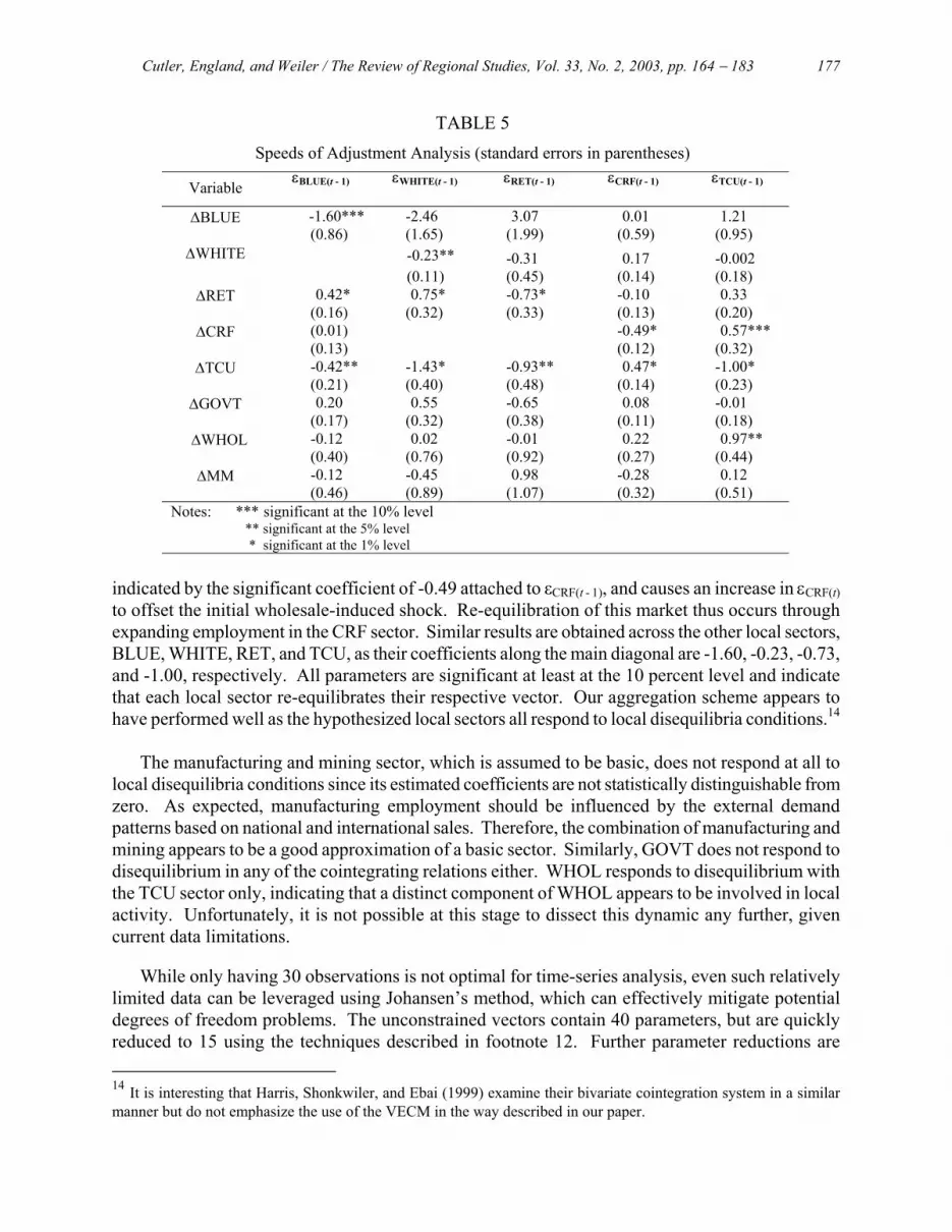
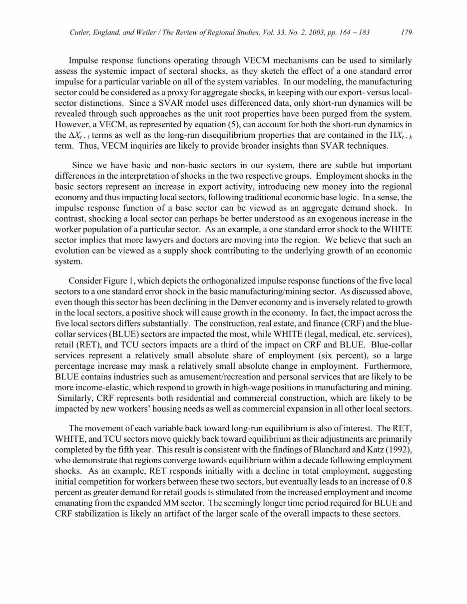
Consider Figure 1, which depicts the orthogonalized impulse response functions of the five local
sectors to a one standard error shock in the basic manufacturing/mining sector. As discussed above, even though this sector has been declining in the Denver economy and is inversely related to growth in the local sectors, a positive shock will cause growth in the economy. In fact, the impact across the five local sectors differs substantially. The construction, real estate, and finance (CRF) and the blue-collar services (BLUE) sectors are impacted the most, while WHITE (legal, medical, etc. services), retail (RET), and TCU sectors impacts are a third of the impact on CRF and BLUE. Blue-collar services represent a relatively small absolute share of employment (six percent), so a large percentage increase may mask a relatively small absolute change in employment. Furthermore, BLUE contains industries such as amusement/recreation and personal services that are likely to be more income-elastic, which respond to growth in high-wage positions in manufacturing and mining. Similarly, CRF represents both residential and commercial construction, which are likely to be impacted by new workers’ housing needs as well as commercial expansion in all other local sectors.
The movement of each variable back toward long-run equilibrium is also of interest. The RET,
WHITE, and TCU sectors move quickly back toward equilibrium as their adjustments are primarily completed by the fifth year. This result is consistent with the findings of Blanchard and Katz (1992), who demonstrate that regions converge towards equilibrium within a decade following employment shocks. As an example, RET responds initially with a decline in total employment, suggesting initial competition for workers between these two sectors, but eventually leads to an increase of 0.8 percent as greater demand for retail goods is stimulated from the increased employment and income emanating from the expanded MM sector. The seemingly longer time period required for BLUE and CRF stabilization is likely an artifact of the larger scale of the overall impacts to these sectors.
Cutler, England, and Weiler / The Review of Regional Studies, Vol. 33, No. 2, 2003, pp. 164 − 183 180
FIGURE 1
Orthogonalized Impulse Response(s) to one S.E. shock in the equation for
LMM
LBLUE
LWHITE
LRET
LCRF
LTCU
Horizon
-0.01
0.00
0.01
0.02
0.03
0.04
0 5 10 15 20 25 30 35 40 45 5050
FIGURE 2
Orthogonalized Impulse Response(s) to one S.E. shock in the equation for
LWHIT
LBLUE
LWHITE
LRET
LCRF
LTCU
Horizon
0.00
0.05
0.10
0.15
0 5 10 15 20 25 30 35 40 45 5050
FIGURE 3
Orthogonalized Impulse Response(s) to one S.E. shock in the equation forLRET
LBLUE
LWHITE
LRET
LCRF
LTCU
Horizon
-0.005
-0.010
-0.015
0.000
0.005
0.010
0.015
0 5 10 15 20 25 30 35 40 45 5050

Cutler, England, and Weiler / The Review of Regional Studies, Vol. 33, No. 2, 2003, pp. 164 − 183 181
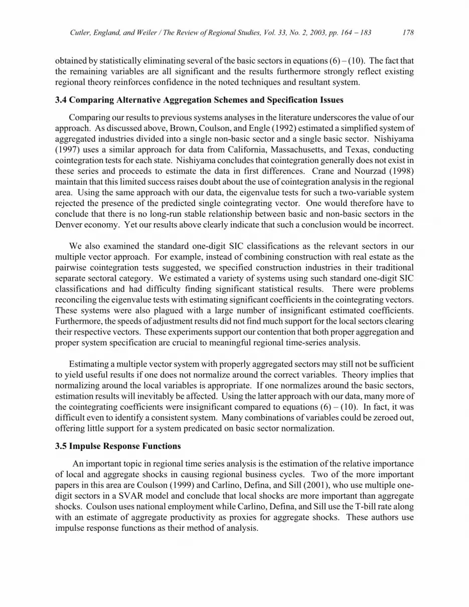
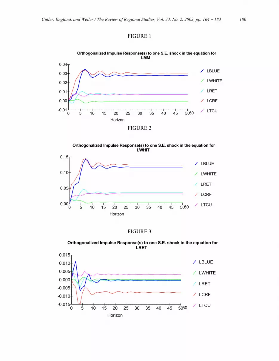
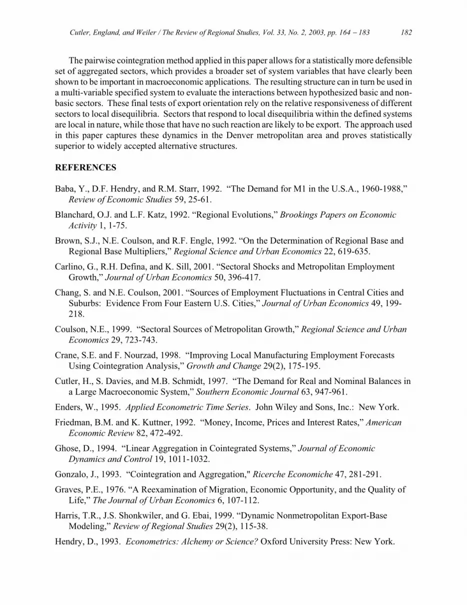
Figures 2 and 3 represent the impulse responses of the five local sectors stemming from shocks to WHITE and RET. As argued above, it may be appropriate to consider these as supply shocks. As expected, a shock to the WHITE sector has a much greater impact to the local sectors than does a shock to the RET sector. Since wages are much higher for legal, medical, and business services than for retail jobs, typical household induced spending effects understandably cause WHITE’s local sector impacts to be at least three times larger than comparable RET impacts. In addition, WHITE makes up approximately 31 percent of the work force, so a one standard error shock is relatively large, highlighting the likely substantial impacts of a shock to this sector.
One additional comparison is worth noting. The long-run impacts of a manufacturing shock are
smaller than that of the WHITE sector, which appears to be contrary to traditional economic base conclusions. However, this finding may reflect the unusually large role of high-skill, high-income services in the rapidly evolving Denver metropolitan area, alongside the noted relative senescence of traditional manufacturing and mining sectors during the same period. The former dynamic is consistent with amenity-driven high-income migration discussed in Graves’ (1976) seminal work.
Our results are also consistent with Coulson’s seminal (1999) findings. Coulson examines five
SMSAs, including Denver, and concludes generally that the service sector has a greater impact than the manufacturing sector in causing business cycle behavior. In addition, he finds that the impact of manufacturing is greater than that of the trade sector. Carlino, Defina, and Sill (2001) find more variation across five different SMSAs, with aggregate (i.e., manufacturing) and local (i.e., trade) having similar impacts for three of the five SMSAs examined. They maintain that using annual data results reduces the impact of local shocks relative to aggregate shocks; the importance of local shocks is only apparent in higher frequency (monthly or quarterly) data. However, both our annual results and Coulson’s monthly results yield similar conclusions regarding the relative impact of local and aggregate shocks. These findings offer contrary evidence to the Carlino, Defina, and Sill claim. A tentative hypothesis that emerges from this contrast is that proper aggregation can produce consistent results across a range of data periodicities.
4. CONCLUSIONS
While previous research has hinted at the potential utility of cointegration techniques in assessing regional systems, these studies’ limited success has slowed regional cointegration applications. This paper proposes that the lessons drawn from macroeconomic applications can help solve regional research’s cointegration struggles. In particular, the joint hurdles of sufficient disaggregation and proper specification of systems are critical to achieving a useful system for statistical analysis.
Categorizing export and local industrial bases is a standard technique in regional economic
analysis. Yet the procedure for such determinations is often surprisingly loose, with few criteria to test particular dichotomies. Furthermore, the reliance on standard aggregations such as the one-digit SIC structure could lead to significant aggregation biases, as industrial structures are likely to differ across regions. This paper proposes that cointegration can provide a useful set of techniques to not only properly aggregate and specify the industrial structure of a region, but also assess the export versus local character of sectors.
Cutler, England, and Weiler / The Review of Regional Studies, Vol. 33, No. 2, 2003, pp. 164 − 183 182
The pairwise cointegration method applied in this paper allows for a statistically more defensible set of aggregated sectors, which provides a broader set of system variables that have clearly been shown to be important in macroeconomic applications. The resulting structure can in turn be used in a multi-variable specified system to evaluate the interactions between hypothesized basic and non-basic sectors. These final tests of export orientation rely on the relative responsiveness of different sectors to local disequilibria. Sectors that respond to local disequilibria within the defined systems are local in nature, while those that have no such reaction are likely to be export. The approach used in this paper captures these dynamics in the Denver metropolitan area and proves statistically superior to widely accepted alternative structures. REFERENCES Baba, Y., D.F. Hendry, and R.M. Starr, 1992. “The Demand for M1 in the U.S.A., 1960-1988,”
Review of Economic Studies 59, 25-61.
Blanchard, O.J. and L.F. Katz, 1992. “Regional Evolutions,” Brookings Papers on Economic Activity 1, 1-75.
Brown, S.J., N.E. Coulson, and R.F. Engle, 1992. “On the Determination of Regional Base and Regional Base Multipliers,” Regional Science and Urban Economics 22, 619-635.
Carlino, G., R.H. Defina, and K. Sill, 2001. “Sectoral Shocks and Metropolitan Employment Growth,” Journal of Urban Economics 50, 396-417.
Chang, S. and N.E. Coulson, 2001. “Sources of Employment Fluctuations in Central Cities and Suburbs: Evidence From Four Eastern U.S. Cities,” Journal of Urban Economics 49, 199-218.
Coulson, N.E., 1999. “Sectoral Sources of Metropolitan Growth,” Regional Science and Urban Economics 29, 723-743.
Crane, S.E. and F. Nourzad, 1998. “Improving Local Manufacturing Employment Forecasts Using Cointegration Analysis,” Growth and Change 29(2), 175-195.
Cutler, H., S. Davies, and M.B. Schmidt, 1997. “The Demand for Real and Nominal Balances in a Large Macroeconomic System,” Southern Economic Journal 63, 947-961.
Enders, W., 1995. Applied Econometric Time Series. John Wiley and Sons, Inc.: New York.
Friedman, B.M. and K. Kuttner, 1992. “Money, Income, Prices and Interest Rates,” American Economic Review 82, 472-492.
Ghose, D., 1994. “Linear Aggregation in Cointegrated Systems,” Journal of Economic Dynamics and Control 19, 1011-1032.
Gonzalo, J., 1993. “Cointegration and Aggregation," Ricerche Economiche 47, 281-291.
Graves, P.E., 1976. “A Reexamination of Migration, Economic Opportunity, and the Quality of Life,” The Journal of Urban Economics 6, 107-112.
Harris, T.R., J.S. Shonkwiler, and G. Ebai, 1999. “Dynamic Nonmetropolitan Export-Base Modeling,” Review of Regional Studies 29(2), 115-38.
Hendry, D., 1993. Econometrics: Alchemy or Science? Oxford University Press: New York.
Cutler, England, and Weiler / The Review of Regional Studies, Vol. 33, No. 2, 2003, pp. 164 − 183 183
Hoen, A.R., 2002. “Identifying Linkages with a Cluster-Based Methodology,” Economic Systems Research 14(2), 131-146.
Isserman, A.M., 1980. “Estimating Export Activity in a Regional Economy: A Theoretical and Empirical Analysis of Alternative Methods,” International Regional Science Review 5(2), 155-184.
Johansen, S., 1988. “Statistical Analysis of Cointegration Vectors,” Journal of Economic Dynamics and Control 12, 231-254.
_______, 1992. “Cointegration in Partial Systems and the Efficiency of Single-Equation Analysis,” Journal of Econometrics 52, 389-402.
_______, 1995. Likelihood-Based Inference in Cointegrated Vector Auto-Regressive Models. Oxford University Press: New York.
Jung, C., K. Krutilla, and R. Boyd, 1997. “Aggregation Bias in Natural Resource Price Composites: The Forestry Case,” Resource and Energy Economics 20, 65-73.
Martin-Alvarez, F.J., V.J. Cano-Fernandez, and J.J. Caceres-Hernandez, 1999. “The Introduction of Seasonal Unit Roots and Cointegration to Test Index Aggregation Optimality: An Application to a Spanish Farm Price Index,” Empirical Economics 24, 403-414.
Nichols, D. and D. Mushinski, 2003. “Identifying Export Industries Using Parametric Density Functions,” International Regional Science Review 26, 68-85.
Nishiyama, Y., 1997. “Exports’ Contribution to Economic Growth: Empirical Evidence for California, Massachusetts, and Texas, Using Employment Data,” Journal of Regional Science 37(1), 99-125.
Phillips, P.C.B., 1991. “Optimal Inference in Cointegrated Systems,” Econometrica 59, 283-306.
Shoesmith, G.L., 1992. “Non-cointegration and Causality: Implications for VAR Modeling,” International Journal of Forecasting 8(2), 187-99.
Stock, J.H. and M.W. Watson, 1993. “A Simple Estimator of Cointegrating Vectors in Higher Order Integrated Systems,” Econometrica 61, 783-820.