Inference on the Cointegration Rank inFractionally Integrated Processes∗

Jorg BreitungHumboldt University Berlin

Uwe HasslerFree University Berlin

Abstract

For univariate time series we suggest a new variant of efficient scoretests against fractional alternatives. This test has three importantmerits. First, by means of simulations we observe that it is superiorin terms of size and power in some situations of practical interest.Second, it is easily understood and implemented as a slight modifica-tion of the Dickey-Fuller test, although our score test has a limitingnormal distribution. Third and most important, our test generalizesto multivariate cointegration tests just as the Dickey-Fuller test does.Thus it allows to determine the cointegration rank of fractionally in-tegrated time series. It does so by solving a generalized eigenvalueproblem of the type proposed by Johansen (1988). However, the li-miting distribution of the corresponding trace statistic is χ2, wherethe degrees of freedom depend only on the cointegration rank underthe null hypothesis. The usefulness of the asymptotic theory for finitesamples is established in a Monte Carlo experiment.

∗The first author gratefully acknowledges financial support from the Sonderforschungs-bereich 373 of the DFG. We thank Luis Gil-Alana, Eiji Kurozumi, three anonymous refer-ees and the participants of the Cardiff Conference on Long Memory and Nonlinear TimeSeries, July 9th-11th 2000, for helpful comments and suggestions.

1

1 Introduction

With his seminal paper introducing fractional integration and cointegration

Granger (1981) opened a productive research avenue. Since then cointe-

gration techniques have become standard in the econometrician’s tool kit.

Fractional cointegration techniques, however, are still to be developed, see

Robinson (1994a) and Baillie (1996) for overviews on fractional integration

in econometrics. A vector of time series variables is called fractionally cointe-

grated if the variables are integrated of order d > 0.5 and there exists a linear

combination of the variables with a smaller degree of integration d− b. The

properties of fractionally cointegrated systems are analyzed by Cheung and

Lai (1993), Jeganathan (1999), Robinson and Marinucci (1998), and Tsay

(2000). Empirical applications can be found in, e.g., Cheung and Lai (1993),

Booth and Tse (1995) and Masih and Masih (1995, 1998), Baillie and Boller-

slev (1994) and Dueker and Startz (1998). Recently, Andersson and Greden-

hoff (1999) investigated experimentally the behaviour of the likelihood ratio

statistic suggested by Johansen (1988). Given observations integrated of or-

der one and fractional cointegration they observe that the likelihood ratio

test has a fairly high power. In contrast, Gonzalo and Lee (1998, 2000) show

that the true null of no cointegration will be rejected spuriously more often

than the nominal level given the observed series are fractionally integrated

of order d = 1. This is one motivation for our present paper.

The starting point of our analysis is a univariate score test for integration

against fractional alternatives. We propose a regression variant of the score

statistic suggested by Robinson (1991, 1994b), Agiakloglou and Newbold

(1994), and Tanaka (1999). This test can be understood and implemented

as a slight modification of the Dickey-Fuller test (Dickey and Fuller 1979),

although it has a limiting normal distribution. To test against fractional

cointegration we generalize the test in the same manner as Johansen’s like-

lihood ratio test for the cointegration rank can be seen as a generalisation

of the Dickey-Fuller test. By solving a generalized eigenvalue problem ana-

logous to that by Johansen (1988) we suggest to determine the cointegration

2

rank of fractionally integrated time series. The limiting distribution depends

neither on the order of integration of the series nor on the order of integration

of the deviations from the long-run relationships. Instead, the asymptotic

distribution is χ2, where the degrees of freedom depend on the cointegration

rank under the null hypothesis. This result is also valid in case of classi-

cal cointegration where the series are integrated of order d = 1 with linear

combinations integrated of order zero.

The rest of this paper is organized as follows. Section 2 introduces our

variant of the univariate score statistic that can be implemented as a modifi-

cation of the Dickey-Fuller test. Section 3 extends the analysis to multivari-

ate processes that are not cointegrated, whereas in the fourth section a test

for the fractional cointegration rank is suggested. The fifth section presents

some Monte Carlo evidence on the performance of our tests in finite samples

relative to competing procedures. Concluding remarks can be found in the

final section. All proofs are relegated to the Appendix.

2 Testing against fractional alternatives

Assume that we want to test the hypothesis that a univariate time series is

an I(d) process, (1−L)dyt = εt, t = 1, 2, . . . , T , where εt is white noise with

E(εt) = 0 and E(ε2t ) = σ2, against the alternative that yt is I(d + θ). This

test is equivalent to a test of the hypothesis that xt ≡ (1 − L)dyt is white

noise against the alternative that xt is I(θ) with θ = 0.

Robinson (1991, 1994b) and Tanaka (1999) derive score statistics for this

test problem. We adopt their model, which corresponds to so-called fraction-

ally integrated noise, see Hosking (1981),

(1− L)d+θyt = εt , t = 1, . . . , T , (1)

where L denotes the lag operator and (1 − L)d+θ is given by the usual ex-

pansion. It is assumed that εt ∼ i.i.d.(0, σ2) and yt = 0 for t ≤ 0. The

null hypothesis in this framework is given by H0 : θ = 0. We further follow

Robinson (1991, 1994b) and Tanaka (1999) and assume that εt is normally

3

distributed in order to obtain the score statistic, although the asymptotic

theory does not require this assumption. The log-likelihood function is given

by

L(θ, σ) = −T

2log(2πσ2)− 1

2σ2

T∑t=1

[(1− L)d+θyt

]2.

The derivative of the log-likelihood function with xt ≡ (1− L)dyt evaluated

at θ = 0 is obtained as, cf. Tanaka (1999, (40)),

∂L(θ, σ)

∂θ

∣∣∣∣θ=0

=1

σ2

T∑t=2

xt

(t−1∑j=1

j−1xt−j

)

=1

σ2

T∑t=2

xtx∗t−1 , (2)

where

x∗t−1 =

t−1∑j=1

j−1xt−j . (3)

Using limT→∞E(x∗T )2 = σ2π2/6, Tanaka (1999) suggests the test statistic

τT =6T

π2

[T−1∑j=1

j−1j

]2

,

where j =∑T

t=j+1 xtxt−j/∑T

t=1 x2t . The same test statistic was proposed by

Robinson (1991) to test against fractionally integrated noise, while Robinson

(1994b) favours a frequency domain approach.

Following Agiakloglou and Newbold (1994) we consider the corresponding

regression statistic that is obtained as the squared t-statistic for φ = 0 in the

regression1

xt = φx∗t−1 + et . (4)

1Agiakloglou and Newbold (1994) suggest to use x(m)t−1 =

∑mj=1 j−1xt−j instead of x∗

t−1,where m is some pre-specified truncation parameter. In our test we avoid the somehowarbitrary specification of m and choose m = t− 1 to be time dependent which gives a teststatistic that is asymptotically equivalent to the tests suggested by Robinson (1994b) andTanaka (1999).

4

This test statistic is obtained by using the outer product of gradients as an

estimate of the Fisher information:

τ ∗T =

(T∑

t=2

xtx∗t−1

)2

σ2e

T∑t=2

x∗2t−1

, (5)

where σ2e is the usual regression estimate for the variance of et.

It is interesting to compare the test statistic τ ∗T with the well known

Dickey-Fuller test. If d = 1 define xt = yt − yt−1 and xt−1 = yt−1 = xt−1 +

xt−2+ · · ·+x1, and the Dickey-Fuller regression corresponding to (4) is given

by

xt = φxt−1 + et .

The only difference between our statistic in (5) and the Dickey-Fuller statistic

is the introduction of the weights j−1 in (3). A similar generalization of the

Dickey-Fuller test to a fractional framework has recently been proposed by

Dolado, Gonzalo and Mayoral (1999). Let d∗ = d + θ∗ be some prespecified

value for the fractional parameter. Then Dolado et al. (1999) define xt =

(1− L)dyt and xt−1 = (1− L)d∗yt−1, where the latter is given by expansion

of the fractional filter. The Dickey-Fuller test results as a special case with

d = 1 and d∗ = 0. For 0 ≤ d∗ < 0.5 the test has a nonstandard limiting

distribution (cf. Dolado et al. 1999). In contrast, the score statistic (5) is

asymptotically χ2 distributed with one degree of freedom.

Theorem 1: Let yt be given in (1), where εt is white noise with E(ε2t ) < ∞.

Then, for θ = 0, it holds that τ ∗T = τT + op(1) and, therefore, τ ∗Td→ χ2(1) as

T → ∞.

To allow for short memory dynamics of xt we adopt the approach of the

REG test suggested by Agiakloglou and Newbold (1994). Assume that xt

is a stable AR(p) process. In this case, one computes the residuals from an

5

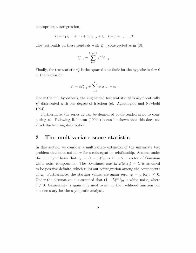
appropriate autoregression,

xt = a1xt−1 + · · ·+ apxt−p + εt , t = p+ 1, . . . , T.

The test builds on these residuals with ε∗t−1 constructed as in (3),

ε∗t−1 =

t−p−1∑j=1

j−1εt−j .

Finally, the test statistic τ ∗T is the squared t-statistic for the hypothesis φ = 0

in the regression

εt = φε∗t−1 +

p∑i=1

ψi xt−i + et .

Under the null hypothesis, the augmented test statistic τ ∗T is asymptotically

χ2 distributed with one degree of freedom (cf. Agiakloglou and Newbold

1994).

Furthermore, the series xt can be demeaned or detrended prior to com-

puting τ ∗T . Following Robinson (1994b) it can be shown that this does not

affect the limiting distribution.

3 The multivariate score statistic

In this section we consider a multivariate extension of the univariate test

problem that does not allow for a cointegration relationship. Assume under

the null hypothesis that xt = (1 − L)dyt is an n × 1 vector of Gaussian

white noise components. The covariance matrix E(xtx′t) = Σ is assumed

to be positive definite, which rules out cointegration among the components

of yt. Furthermore, the starting values are again zero, yt = 0 for t ≤ 0.

Under the alternative it is assumed that (1 − L)d+θyt is white noise, where

θ = 0. Gaussianity is again only used to set up the likelihood function but

not necessary for the asymptotic analysis.

6

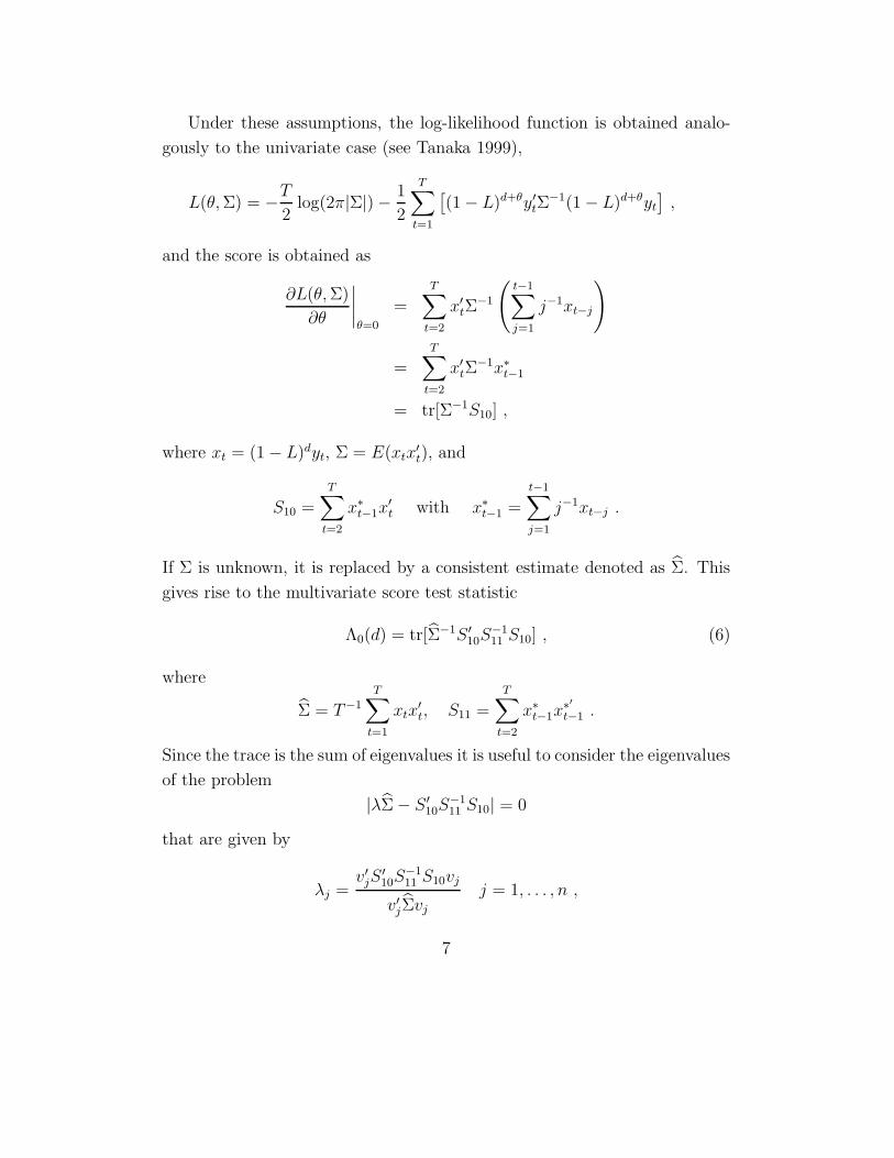
Under these assumptions, the log-likelihood function is obtained analo-

gously to the univariate case (see Tanaka 1999),

L(θ,Σ) = −T

2log(2π|Σ|)− 1

2

T∑t=1

[(1− L)d+θy′tΣ

−1(1− L)d+θyt

],

and the score is obtained as

∂L(θ,Σ)

∂θ

∣∣∣∣θ=0

=

T∑t=2

x′tΣ−1

(t−1∑j=1

j−1xt−j

)

=T∑

t=2

x′tΣ−1x∗t−1

= tr[Σ−1S10] ,

where xt = (1− L)dyt, Σ = E(xtx′t), and

S10 =

T∑t=2

x∗t−1x′t with x∗t−1 =

t−1∑j=1

j−1xt−j .

If Σ is unknown, it is replaced by a consistent estimate denoted as Σ. This

gives rise to the multivariate score test statistic

Λ0(d) = tr[Σ−1S ′10S

−111 S10] , (6)

where

Σ = T−1

T∑t=1

xtx′t, S11 =

T∑t=2

x∗t−1x∗′t−1 .

Since the trace is the sum of eigenvalues it is useful to consider the eigenvalues

of the problem

|λΣ− S ′10S

−111 S10| = 0

that are given by

λj =v′jS

′10S

−111 S10vj

v′jΣvj

j = 1, . . . , n ,

7

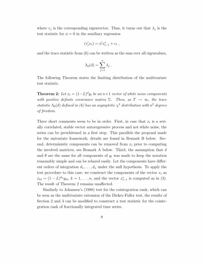
where vj is the corresponding eigenvector. Thus, it turns out that λj is the

test statistic for φ = 0 in the auxiliary regression

(v′jxt) = φ′x∗t−1 + et ,

and the trace statistic from (6) can be written as the sum over all eigenvalues,

Λ0(d) =n∑

j=1

λj .

The following Theorem states the limiting distribution of the multivariate

test statistic.

Theorem 2: Let xt = (1−L)dyt be an n×1 vector of white noise components

with positive definite covariance matrix Σ. Then, as T → ∞, the trace

statistic Λ0(d) defined in (6) has an asymptotic χ2 distribution with n2 degrees

of freedom.

Three short comments seem to be in order. First, in case that xt is a seri-

ally correlated, stable vector autoregressive process and not white noise, the

series can be prewhitened in a first step. This parallels the proposal made

for the univariate framework; details are found in Remark B below. Sec-

ond, deterministic components can be removed from xt prior to computing

the involved matrices, see Remark A below. Third, the assumption that d

and θ are the same for all components of yt was made to keep the notation

reasonably simple and can be relaxed easily. Let the components have differ-

ent orders of integration d1, . . . , dn under the null hypothesis. To apply the

test procedure to this case, we construct the components of the vector xt as

xkt = (1− L)dkykt, k = 1, . . . , n, and the vector x∗t−1 is computed as in (3).

The result of Theorem 2 remains unaffected.

Similarly to Johansen’s (1988) test for the cointegration rank, which can

be seen as the multivariate extension of the Dickey-Fuller test, the results of

Section 2 and 3 can be modified to construct a test statistic for the cointe-

gration rank of fractionally integrated time series.

8

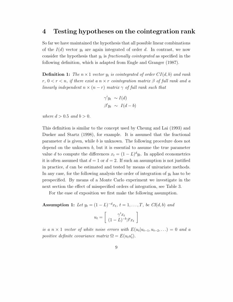
4 Testing hypotheses on the cointegration rank

So far we have maintained the hypothesis that all possible linear combinations

of the I(d) vector yt are again integrated of order d. In contrast, we now

consider the hypothesis that yt is fractionally cointegrated as specified in the

following definition, which is adapted from Engle and Granger (1987).

Definition 1: The n× 1 vector yt is cointegrated of order CI(d, b) and rank

r, 0 < r < n, if there exist a n× r cointegration matrix β of full rank and a

linearly independent n× (n− r) matrix γ of full rank such that

γ′yt ∼ I(d)

β ′yt ∼ I(d− b)

where d > 0.5 and b > 0.

This definition is similar to the concept used by Cheung and Lai (1993) and

Dueker and Startz (1998), for example. It is assumed that the fractional

parameter d is given, while b is unknown. The following procedure does not

depend on the unknown b, but it is essential to assume the true parameter

value d to compute the differences xt = (1− L)dyt. In applied econometrics

it is often assumed that d = 1 or d = 2. If such an assumption is not justified

in practice, d can be estimated and tested by means of univariate methods.

In any case, for the following analysis the order of integration of yt has to be

prespecified. By means of a Monte Carlo experiment we investigate in the

next section the effect of misspecified orders of integration, see Table 3.

For the ease of exposition we first make the following assumption.

Assumption 1: Let yt = (1− L)−dxt, t = 1, . . . , T , be CI(d, b) and

ut =

[γ′xt

(1− L)−bβ ′xt

]is a n × 1 vector of white noise errors with E(ut|ut−1, ut−2, . . .) = 0 and a

positive definite covariance matrix Ω = E(utu′t).

9

The assumption that ut is white noise is made to facilitate the proof of the

main result, and it will be relaxed below (see Remark B).

Following Johansen (1995) we test hypotheses on the cointegration rank

based on the sum of the n− r smallest eigenvalues of the problem:

|λS11 − S10Σ−1S ′

10| = 0 ,

or, equivalently,

|λΣ− S ′10S

−111 S10| = 0 , (7)

where Σ, S10 and S11 are defined as in (6). As in the univariate case, we

replace the partial sum yt−1 = x1 + · · ·+xt−1 used in Johansen (1988) by the

weighted sum x∗t−1 =∑t−1

j=1 j−1xt−j . Furthermore, for the special case r = 0

(no cointegration) the corresponding trace statistic turns out to be identical

to the multivariate score statistic Λ0(d) defined in (6).

In the following theorem, the null distribution of the test statistic for the

cointegration rank is given.

Theorem 3: Let yt be CI(d, b) with d > 0.5 and b > 0. Under Assumption

1 and the hypothesis H0 : r = r0 the trace statistic

Λr0(d) =

n−r0∑j=1

λj ,

where λ1 ≤ · · · ≤ λn are the ordered eigenvalues of problem (7), has an

asymptotic χ2 distribution with (n − r0)2 degrees of freedom. Under the al-

ternative H1 : r0 < r the test statistic diverges to infinity at rate T .

Remark A: To allow for a non-zero mean we assume E(xt) = θ′dt, where

dt is a k× 1 vector of deterministic functions like a constant, a time trend or

dummy variables, and θ is a k×n matrix of parameters. Since xt = (1−L)dyt

is assumed to be stationary, the least-squares regression of xt on dt yields a√T−consistent estimate of θ. The test statistic can be constructed by using

the adjusted series xt = xt − θ′dt instead of the original observations xt.

Following Robinson (1994b) it can be shown that the limiting distribution is

10

not affected when the time series is adjusted for deterministic terms like a

constant or a linear time trend.

Remark B: To allow for possible short run dynamics, the approach of Agiak-

loglou and Newbold (1994) can be adapted. Assume that γ′xt has a VAR(p)

representation.2 In this case the test statistic is constructed by using the

prewhitened series, that is, the residuals εt from a vector autoregression of

xt on xt−1, . . . , xt−p:

xt = A1xt−1 + · · ·+ Apxt−p + εt , t = p+ 1, . . . , T.

Analogously to the univariate case we compute

ε∗t−1 =

t−p−1∑j=1

j−1εt−j ,

which is used to define ε∗t−1 = [ε∗′

t−1, x′t−1, . . . , x

′t−p]

′. Now, εt and ε∗t−1 are

employed when computing the matrices in (7),

Σ = T−1T∑

t=1

εtε′t , S10 =

T∑t=2

ε∗t−1ε′t , S11 =

T∑t=2

ε∗t−1ε∗t−1

′ .

Finally, the corresponding eigenvalues are determined from

|λΣ− S ′10S

−111 S10| = 0 ,

and the resulting trace statistic has the same asymptotic χ2 distribution as

in Theorem 3.

Remark C: The assumuption that b is one and the same for all r cointegrat-

ing vectors was made only for notational convenience. Indeed, the procedure

allows for different values b1, . . . , br. Since the null distribution of the test

statistic does not depend on b the results of Theorem 3 are also valid for the

case of different values b1, . . . , br.

2In the proof of Theorem 3 it is shown that asymptotically the test statistic doesnot depend on the component β′xt. Therefore, we do not need to specify the short rundynamics for β′xt.

11

5 Finite sample properties

Since our multivariate test is based on a generalization of the regression

variant of the univariate score statistic, it is interesting to compare the per-

formance of our variant with other univariate tests against fractional alterna-

tives. We consider the two-sided test problem with the null hypothesis d = 1

against the alternative d1 = d+ θ = 1.

For our Monte Carlo experiments we simulated fractionally integrated

noise according to Hosking (1984),

(1− L)d1−1zt = εt, εt ∼ iidN (0, 1), and 0.7 ≤ d1 ≤ 1.3 . (8)

The final series are obtained by computing the partial sum yt =∑t

j=1 zj .

The Monte Carlo comparison includes Robinson’s (1994b) frequency do-

main score statistic RT , Tanaka’s (1999) time domain statistic τT , the REG(m)

statistic by Agiakloglou and Newbold (1994) relying on x(m)t−1 =

∑mj=1 j

−1xt−j

instead of x∗t−1, and our variant τ ∗T defined in (5). With the REG test we tried

m = 10 and m = 20 and observed only marginal differences. Here, only the

slightly more powerful case m = 10 is reported. Furthermore, the fractional

Dickey-Fuller (FDF) test suggested by Dolado, Gonzalo and Mayoral (1999)

is applied using d∗ = d1 under the alternative, and d∗ = 0.9 under the null

hypothesis. All tests are computed by using demeand series xt.

For the two-sided test problem all statistics are asymptotically χ2 dis-

tributed with one degree of freedom. In Table 1 we report the rejection

frequencies using a nominal significance level of 0.05. All results rely on 5000

Monte Carlo replications.

The results presented in Table 1 can be summarized as follows. The

actual sizes of RT and τT are slightly below the nominal size, while the other

tests are only slightly above. For T = 250, REG(10) and τ ∗T are closest to

the nominal level. Our findings with respect to the power are as follows.

For T = 100 and d1 < 1 our Dickey-Fuller type score test dominates all

other tests. The REG(10) test is only slightly less powerful. For T = 100

and d1 > 1, Tanaka’s (1999) test performs best, the other score tests behave

12

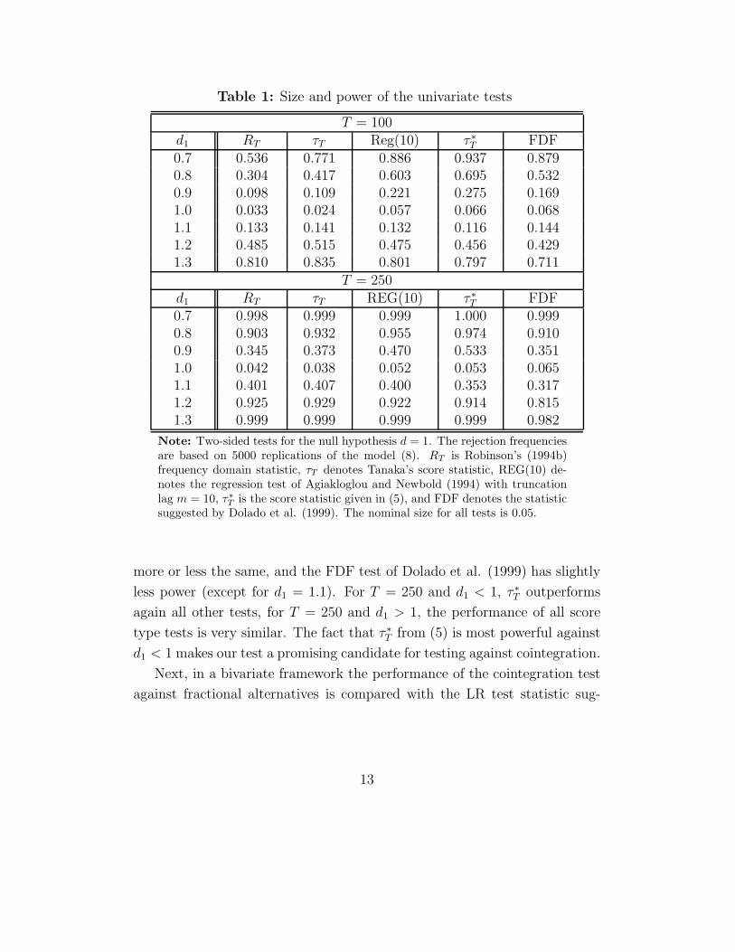
Table 1: Size and power of the univariate tests

T = 100d1 RT τT Reg(10) τ ∗T FDF0.7 0.536 0.771 0.886 0.937 0.8790.8 0.304 0.417 0.603 0.695 0.5320.9 0.098 0.109 0.221 0.275 0.1691.0 0.033 0.024 0.057 0.066 0.0681.1 0.133 0.141 0.132 0.116 0.1441.2 0.485 0.515 0.475 0.456 0.4291.3 0.810 0.835 0.801 0.797 0.711

T = 250d1 RT τT REG(10) τ ∗T FDF0.7 0.998 0.999 0.999 1.000 0.9990.8 0.903 0.932 0.955 0.974 0.9100.9 0.345 0.373 0.470 0.533 0.3511.0 0.042 0.038 0.052 0.053 0.0651.1 0.401 0.407 0.400 0.353 0.3171.2 0.925 0.929 0.922 0.914 0.8151.3 0.999 0.999 0.999 0.999 0.982

Note: Two-sided tests for the null hypothesis d = 1. The rejection frequenciesare based on 5000 replications of the model (8). RT is Robinson’s (1994b)frequency domain statistic, τT denotes Tanaka’s score statistic, REG(10) de-notes the regression test of Agiakloglou and Newbold (1994) with truncationlag m = 10, τ∗

T is the score statistic given in (5), and FDF denotes the statisticsuggested by Dolado et al. (1999). The nominal size for all tests is 0.05.

more or less the same, and the FDF test of Dolado et al. (1999) has slightly

less power (except for d1 = 1.1). For T = 250 and d1 < 1, τ ∗T outperforms

again all other tests, for T = 250 and d1 > 1, the performance of all score

type tests is very similar. The fact that τ ∗T from (5) is most powerful against

d1 < 1 makes our test a promising candidate for testing against cointegration.

Next, in a bivariate framework the performance of the cointegration test

against fractional alternatives is compared with the LR test statistic sug-

13

gested by Johansen (1988). The data is generated according to the model

y1t = αy1,t−1 + ut , ut = ρut−1 + ε1t , |ρ| < 1y2t = y1t + vt , (1− L)1−bvt = ε2t ,

(9)

where ε1t and ε2t are uncorrelated white noise processes distributed asN(0, 1).

For α = 1 and b > 0, the process has a cointegration relationship with coin-

tegration vector [1,−1]. If α = 0, then y1t is stationary; if in addition

b = 0, then the cointegration rank is one with the “cointegration vector”

[1, 0], whereas for b > 0 the cointegration rank r = 2 results. Furthermore,

for ρ = 0 the process has a VAR(1) representation, whereas for ρ = 0 a

VAR(2) representation is required. In the latter case Johansen’s LR test

includes a lagged difference and the statistic Λr(1) from Theorem 3 against

fractional alternatives (FRAC) is based on the prewhitened series resulting

from the residuals of a VAR(1) model for the first differences (see Remark

B). The sample size is T = 100, and 5000 Monte Carlo replications are used

to compute the rejection frequencies. A nominal significance level of 0.05 is

used for all experiments.

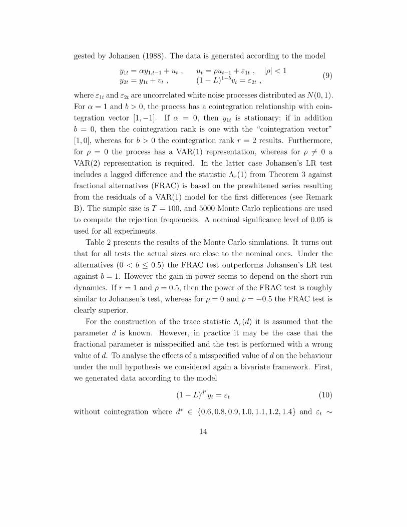
Table 2 presents the results of the Monte Carlo simulations. It turns out

that for all tests the actual sizes are close to the nominal ones. Under the

alternatives (0 < b ≤ 0.5) the FRAC test outperforms Johansen’s LR test

against b = 1. However the gain in power seems to depend on the short-run

dynamics. If r = 1 and ρ = 0.5, then the power of the FRAC test is roughly

similar to Johansen’s test, whereas for ρ = 0 and ρ = −0.5 the FRAC test is

clearly superior.

For the construction of the trace statistic Λr(d) it is assumed that the

parameter d is known. However, in practice it may be the case that the

fractional parameter is misspecified and the test is performed with a wrong

value of d. To analyse the effects of a misspecified value of d on the behaviour

under the null hypothesis we considered again a bivariate framework. First,

we generated data according to the model

(1− L)d∗yt = εt (10)

without cointegration where d∗ ∈ 0.6, 0.8, 0.9, 1.0, 1.1, 1.2, 1.4 and εt ∼

14

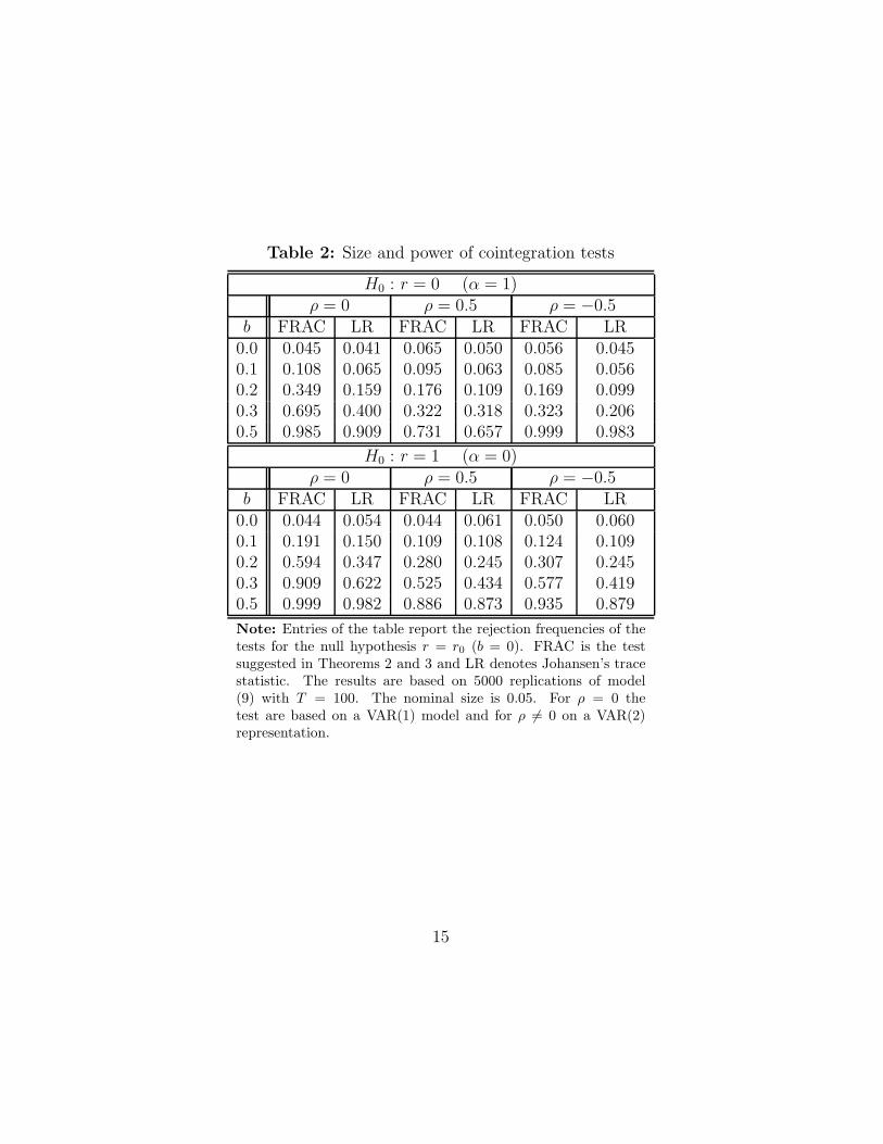
Table 2: Size and power of cointegration tests

H0 : r = 0 (α = 1)ρ = 0 ρ = 0.5 ρ = −0.5

b FRAC LR FRAC LR FRAC LR0.0 0.045 0.041 0.065 0.050 0.056 0.0450.1 0.108 0.065 0.095 0.063 0.085 0.0560.2 0.349 0.159 0.176 0.109 0.169 0.0990.3 0.695 0.400 0.322 0.318 0.323 0.2060.5 0.985 0.909 0.731 0.657 0.999 0.983

H0 : r = 1 (α = 0)ρ = 0 ρ = 0.5 ρ = −0.5

b FRAC LR FRAC LR FRAC LR0.0 0.044 0.054 0.044 0.061 0.050 0.0600.1 0.191 0.150 0.109 0.108 0.124 0.1090.2 0.594 0.347 0.280 0.245 0.307 0.2450.3 0.909 0.622 0.525 0.434 0.577 0.4190.5 0.999 0.982 0.886 0.873 0.935 0.879

Note: Entries of the table report the rejection frequencies of thetests for the null hypothesis r = r0 (b = 0). FRAC is the testsuggested in Theorems 2 and 3 and LR denotes Johansen’s tracestatistic. The results are based on 5000 replications of model(9) with T = 100. The nominal size is 0.05. For ρ = 0 thetest are based on a VAR(1) model and for ρ = 0 on a VAR(2)representation.

15

Table 3: The effect of misspecified values of d

Augmentation lag: p = 1r = 0 r = 1

d∗ FRAC LR FRAC LR0.6 0.901 0.717 0.793 0.6860.8 0.318 0.157 0.288 0.2400.9 0.108 0.066 0.111 0.1151.0 0.054 0.047 0.047 0.0611.1 0.111 0.095 0.091 0.0771.2 0.282 0.212 0.226 0.1531.4 0.384 0.505 0.287 0.354

Augmentation lag: p = 4r = 0 r = 1

d∗ FRAC LR FRAC LR0.6 0.378 0.270 0.265 0.3690.8 0.137 0.093 0.100 0.1460.9 0.097 0.071 0.055 0.0951.0 0.090 0.074 0.046 0.0691.1 0.119 0.100 0.051 0.0751.2 0.154 0.148 0.071 0.1031.4 0.197 0.243 0.091 0.158

Note: The table displays the empirical sizes for a bivariate systemwith elements integrated of order I(d∗). The tests are based onthe assumption that the series are integrated of order d = 1. Theaugmentation lag p is the number of lagged differences in the VARequations. The nominal size for all tests is 0.05 and T = 100.

16

iidN (0, I2). In this specification, the elements of yt are I(d∗) and there is no

cointegration relationship (r = 0). Second, to test the true null hypothesis

r = 1, we generated the first component as (1−L)d∗y1t = ε1t and the second

one as y2t = y1t+ε2t, where ε1t and ε2t are mutually uncorrelated white noise

sequences.

The tests are performed by assuming d = 1. From the simulation results

presented in Table 3 it turns out that in particular for a test of r = 0 a

misspecified value of d can lead to substantial size distortions of the tests.

For a test of r = 0 the Johansen’s LR test appears to be more robust against

a misspecified fractional parameter, whereas for a test of r = 1 with four

lagged differences, the FRAC test turns out to be more robust.

It is important to note that a misspecification of the integration parameter

implies that the errors of the system are serially correlated. Thus, the effect of

misspecification on the null distribution of the test is reduced by accounting

for short-run dynamics of the errors. Comparing the results in Table 3 for

p = 1 (upper panel) and p = 4 (lower panel), it turns out indeed that the

size distortions can be reduced by choosing a large lag order of the VAR

representation. However, a large lag order will lead to a loss of power so that

it is important to carefully specify the fractional parameter. To this end, the

univariate tests discussed in Section 2 can be used to test the supposed value

of the fractional parameter d.

6 Concluding remarks

We modified the efficient score tests by Robinson (1991, 1994b), Agiakloglou

and Newbold (1994) and Tanaka (1999) for the fractional order of integration

of univariate time series in such a way that the statistic can be computed from

a Dickey-Fuller type regression. The test relies on a limiting χ2 distribution

with one degree of freedom.

In this paper we suggest a straightforward extension of the univariate

test to a multivariate setup. It allows to determine the cointegration rank

of possibly fractionally integrated series, where the error correction terms

17

may be fractionally integrated as well. Just like Johansen’s (1988) LR test

statistic can be seen as a generalization of the univariate Dickey-Fuller test,

our test is a multivariate version of the regression based score statistic.

In the multivariate framework the statistic builds on eigenvalues from

a generalized eigenvalue problem, however, under the null hypothesis of r

linearly independent cointegrating vectors the limiting distribution is χ2.

The asymptotic null distribution only depends on the cointegration rank

under the null hypothesis and is affected neither by the potentially fractional

order of integration of the series (which must be known, however) nor by

the possibly fractional order of integration for the deviations of the long-run

relationship.

Although the new procedure is quite general in that it allows for fractional

integration and cointegration, our test is based on a severe restriction. It

requires that all n series are integrated of some known order d (or dk, k =

1, . . . , n). In applied work it is often justified to assume that d = 1 or d = 2. If

this is not the case, d can be estimated and tested in a univariate framework.

This may, of course, result in some misspecification of d, which implies that

the errors of the multivariate system are serially correlated. Thus, the effect

of misspecified orders of integration on the null distribution of the test can be

reduced by accounting for short-run dynamics by means of lagged variables.

However, a large lag order will reduce power as well. Therefore, our test

relies on a careful specification of the order of integration. One possibility to

relax this assumption of known d might be to compute the test statistic with

an estimated order d and use bootstrap critical values (see Davidson 2000).

It seems worthwhile to study such a strategy in future.

18

Appendix

Proof of Theorem 1:

There are two differences between the test statistics τ ∗T and τT , which can be

rewritten as

τT =6

Tπ2σ4

(T∑

t=2

xtx∗t−1

)2

, σ2 = T−1T∑

t=1

x2t .

First, the statistic τ ∗T uses T−1∑

(x∗t−1)2, whereas Tanaka’s test statistic τT is

based on the expected value σ2π2/6. Second, the estimators for the variance

σ2 are different.

Notice that the square summability∑∞

j=1 j−2 = π2/6 implies that x∗t−1 is

asymptotically stationary with V (x∗t−1) → σ2 π2/6 for t → ∞, and ergodic,

see Hannan (1970, p. 204). Thus T−1∑

(x∗t−1)2 converges in probability to

σ2 π2/6, see Hannan (1970, p. 203).

Furthermore it is easy to verify that

σ2e = T−1

T∑t=2

(xt − φx∗t−1)2 = T−1

T∑t=2

x2t + op(1) = σ2 + op(1) .

It follows that τ ∗T = τT + op(1).

Proof of Theorem 2:

Let S10 = Σ−1/2S10, so that the test statistic can be rewritten as Λ0(d) =

tr[S ′10S

−111 S10]. It is not difficult to show that

Λ0(d) = tr[S ′10S

−111 S10]

= vec(S10)′(In ⊗ S−1

11 )vec(S10) .

Since vt = vec(Σ−1/2xtx∗t−1

′) is a martingale difference sequence with E(vt|vt−1,

vt−2, . . .) = 0 it follows from Theorem 5.24 of White (1984) that

T−1/2vec(S10) = T−1/2T∑

t=2

vtd−→ N

(0, In ⊗ lim

T→∞E(x∗Tx

∗T′)).

19

Since Σ is a consistent estimator for Σ and T−1S11 converges weakly to the

limit of E(x∗Tx∗T′) , as T → ∞ (see Hannan 1970), it follows that Λ0(d) has

a χ2 limiting distribution with n2 degrees of freedom.

Proof of Theorem 3:

Let γ be a n× (n− r) matrix such that γ′xt is white noise. Furthermore we

multiply γ′xt by the Choleski factor of the inverse of γ′Σγ such that z1t =

(γ′Σγ)−1/2γ′xt has an identity covariance matrix. Under the null hypothesis,

there exists a matrix β such that β ′xt is I(−b). We define

z2t = β ′xt − β ′Σγ(γ′Σγ)−1γ′xt

so that z2t is uncorrelated with z1t. Furthermore, we multiply z2t by the

Choleski factor of the inverse of Σ2 = E(z2tz′2t) so that z2t = Σ

−1/22 z2t has an

identity covariance matrix.

It is convenient to define the matrices Z1 = [z12, · · · , z1T ]′, Z2 = [z22, · · · , z2T ]

′,Z∗

1 = [z∗11, . . . z∗1,T−1]

′, Z∗2 = [z∗21, . . . , z

∗2,T−1]

′, Z∗ = [Z∗1 , Z

∗2 ], and Z = [Z1, Z2],

where

z∗kt =

t−1∑j=1

j−1zk,t−j for k = 1, 2.

The following Lemma presents some asymptotic properties of the moments

that will be used in what follows. Since in some cases the expected values

are complicated expressions, which are not needed to prove the result, we do

not derive the formulae here.

Lemma A.1: Let Zki and Z∗ki denote the i’th columns of Zk and Z∗

k (k =

1, 2). As T → ∞ we have

(i) T−1/2Z ′1iZ

∗1j

d−→ N(0, π2/6) (ii) T−1/2Z ′1iZ2j

d−→ N(0, 1)

(iii) T−1/2Z ′1iZ

∗2j

d−→ N(0, vjj) (iv) T−1Z ′2iZ

∗1j

p−→ τij(v) T−1Z∗

1i′Z∗

1i

p−→ π2/6 (vi) T−1Z ′2iZ

∗2j

p−→ ρij

(vii) T−1Z∗2i′Z∗

2i

p−→ vii (viii) T−1Z∗1i′Z∗

2j

p−→ cij

20

where τij, ρij, vij and cij are the (i, j) elements of the matrices limT→∞E(z2T z∗1T

′),limT→∞E(z2T z

∗2T

′), limT→∞E(z∗2tz∗′2t) and limT→∞E(z∗1tz

∗2t′), respectively.

Proof: (i) Let zki,t and z∗kj,t denote the t’th element of the vectors Zki and

Z∗kj. The sequence ct = z1i,tz

∗1j,t−1 is a martingale difference sequence with

E(ct|xt−1, xt−2, . . .) = 0 and limt→∞E(c2t ) = π2/6. Using the central limit

theorem for martingale difference sequences (e.g. White 1984, p. 128f), it

follows that T−1/2Z ′1iZ

∗1j = T−1/2

∑ct converges to a normally distributed

random variable with expectation zero and variance π2/6. (ii) Since z1i,t and

z2j,t are mutually uncorrelated asymptotically stationary and ergodic time

series (cf. Hannan 1970) it follows from the respective central limit theorem

(cf. White 1984, p. 118f) that T−1/2Z ′1iZ2j is asymptotically normal with

zero mean and unit variance. (iii) Since ct = z1i,tz∗2j,t−1 is a martingale

difference sequence with E(ct|xt−1, xt−2, . . .) = 0, it follows from the central

limit theorem for martingale difference sequences (e.g. White 1984, p. 128f)

that T−1/2∑

ct = T−1/2Z ′1iZ

∗2j has a normal limiting distribution with finite

variance wij. (iv) Since limt→∞E(z2i,tz∗1j,t) = τij is finite, the law of large

numbers for stationary ergodic time series (White 1984, p.42) implies that

T−1Z ′2iZ

∗1j converges in probability to τij . (v) From the proof of Theorem 1

it follows that T−1∑T

t=2(z∗1i,t)

2 converges in probability to π2/6. (vi) Since

limt→∞E(z2i,tz∗2j,t) = ρij is finite, the law of large numbers for stationary

ergodic time series (White 1984, p.42) implies that T−1Z ′2iZ

∗2j converges in

probability to ρij. In a similar manner (vii) and (viii) can be shown.

Now consider the eigenvalue problem (7) which is equivalent to

|λT−1Z ′Z − Z ′Z∗(Z∗′Z∗)−1Z∗′Z| = 0

Using the results of Lemma A.1 it is not difficult to verify that

Z ′Z∗(Z∗′Z∗)−1Z∗′Z =

[Op(1) Op(T

1/2)Op(T

1/2) Op(T )

].

It follows from rule (6) of Sec. 5.3.1 in Lutkepohl (1996) that n−r eigenvaluesare Op(1) and the other r eigenvalues are Op(T ). Let v∗ = [v∗1, . . . , v

∗n−r] =

21

[In−r,−Φ′]′ denote the matrix of re-normalized eigenvectors corresponding

to the smallest n − r eigenvalues that result from the normalization v∗ =

v(v(1))−1, where v(1) is the upper (n−r)× (n−r) block of the original matrix

of eigenvectors v. As the original eigenvectors, the re-normalized eigenvectors

fulfill the equation

[λT−1Z ′Z − Z ′Z∗(Z∗′Z∗)−1Z∗′Z]v∗j = 0

where v∗j = [ı′j,−φ′j ]′ and ıj is the j’th column of In−r and φj is the j’th

column of Φ. From the lower r equations we obtain

λT−1Z ′2(Z(j) − Z2φj)− Z ′

2Z∗(Z∗′Z∗)−1Z∗′(Z1j − Z2φj) = 0 , (11)

where Z1j denotes the j’th column of Z1. Since for j = 1, . . . , n− r the first

term in (11) is Op(1), it follows that

Z ′2Z

∗(Z∗′Z∗)−1Z∗′(Zij − Z2φj) = Op(1) .

Hence,

φj = [Z ′2Z

∗(Z∗′Z∗)−1Z∗′Z2]−1Z ′

2Z∗(Z∗′Z∗)−1Z∗′Z1j +Op(T

−1)

and it is seen that φj is asymptotically equivalent to a 2SLS estimator of φ∗j

in the equation Z1j = Z2φ∗j + ej using the instrumental matrix Z∗. Define

ej = Z1j − Z2φj ,

then the respective eigenvalue results as

λj =e′jZ

∗(Z∗′Z∗)−1Z∗′ej

T−1e′j ej

+ op(1) .

This shows that the eigenvalue is asymptotically equivalent to Sargan’s (1958)

test of over-identifying restrictions. It follows that the numerator can be re-

written as

e′jZ∗(Z∗′Z∗)−1Z∗′ej = Z ′

1jZ∗M∗

ZZ∗′Z1j

22

where

M∗Z = (Z∗′Z∗)−1

−(Z∗′Z∗)−1Z∗′Z2[Z′2Z

∗(Z∗′Z∗)−1Z∗′Z2]−1Z ′

2Z∗(Z∗′Z∗)−1 .

Note that T−1e′j ej converges to one in probability. Since T−1/2Z∗′Z1j has

a limiting standard normal distribution (cf. Lemma A.1 (i) and (iii)), and

T M∗Z is an idempotent matrix with rank n − r, it hence follows that λj is

asymptotically χ2 distributed with n−r degrees of freedom (see Hansen 1982,

Lemma 4.2).

Furthermore, as T−1/2Z∗′Z1j is asymptotically normal and uncorrelated

with T−1/2Z∗′Z1 for j = 8, it follows that Z ′1jZ

∗M∗ZZ

∗′Z1j and Z′1Z

∗M∗ZZ

∗′Z1

are asymptotically independent for j = 8. Thus, the eigenvalues are asymp-

totically independent as well and∑n−r

j=1 λj has a χ2 limiting distribution with

(n− r)2 degrees of freedom.

Under the alternative ej and Z∗ are correlated so that

limT→∞

E(T−1e′jZ∗) = µ∗

eZ = 0 .

Thus, the eigenvalues λj and hence the test statistic are Op(T ) under the

alternative.

23

References

Agiakloglou, Ch., and Newbold, P. (1994), Lagrange Multiplier Tests

for Fractional Difference, Journal of Time Series Analysis 15, 253-262.

Andersson, M.K., and Gredenhoff, M.P. (1999), On the Maximum Like-

lihood Cointegration Procedure under a Fractional Equilibrium Error,

Economics Letters 65, 143-147.

Baillie, R.T. (1996), Long Memory Processes and Fractional Integration in

Econometrics, Journal of Econometrics 73, 5-59.

Baillie, R.T., and Bollerslev, T. (1994), Cointegration, Fractional Coin-

tegration, and Exchange Rate Dynamics, The Journal of Finance 49,

737-745.

Booth, G.G., and Tse, Y. (1995), Long Memory in Interest Rate Future

Markets: A Fractional Cointegration Analysis, The Journal of Future

Markets 15, 563-54.

Cheung, Y.-E., and Lai, K.S. (1993). A Fractional Cointegration Anal-

ysis of Purchasing Power Parity, Journal of Business and Economic

Statistics 11, 103-122.

Davidson, J. (2000), A Model of Fractional Cointegraion, and Tests for

Cointegration Using the Bootstrap, Cardiff Working Paper at

http://www.cf.ac.uk/carbs/davidsonje.

Dickey, D.A., and Fuller, W.A. (1979), Distribution of the Estimators

for Autoregressive Time Series with a Unit Root, Journal of the Amer-

ican Statistical Association 74, 427-431.

Dolado, J.J., Gonzalo, J., and Mayoral, L. (1999), A Fractional Dickey-

Fuller Test, mimeo Universidad Carlos III de Madrid.

24

Dueker, M., and Startz, R. (1998), Maximum-Likelihood Estimation of

Fractional Cointegration with an Application to U.S. and Canadian

Bond Rates, The Review of Economics and Statistics 80, 420-426.

Engle, R.F. and C.W.J. Granger, C.W.J. (1987), Co-integration and

Error Correction: Representation, Estimation, and Testing, Economet-

rica, 55, 251–276.

Gonzalo, J., and Lee, H.-T. (1998), Pitfalls in Testing for Long Run Re-

lationships, Journal of Econometrics 86, 129-154.

Gonzalo, J., and Lee, H.-T. (2000), On the Robustness of Cointegration

Tests when Time Series are Fractionally Integrated, Journal of Applied

Statistics 27, 821-827.

Granger, C.W.J. (1981), Some Properties of Time Series Data and their

Use in Econometric Model Specification, Journal of Econometrics 16,

121-130.

Hannan, E.J. (1970), Multiple Time Series, Wiley, New York.

Hansen, L.P. (1982), Large Sample Properties of Generalized Method of

Moments Estimators, Econometrica 50, 1029-1054.

Hosking, J.R.M. (1981), Fractional Differencing, Biometrika 68, 165-176.

Hosking, J.R.M. (1984), Modeling Persistence in Hydrological Time Series

using Fractional Differencing, Water Resources Research 20, 1898-1908.

Jeganathan, P. (1999), On Asymptotic Inference in Cointegrated Time Se-

ries with Fractionally Integrated Errors, Econometric Theory 15, 583-

621.

Johansen, S. (1988), Statistical Analysis of Cointegration Vectors, Journal

of Economic Dynamics and Control 12, 231-254.

25

Johansen, S. (1995), Likelihood-Based Inference in Cointegrated Vector

Autoregressive Models, Oxford University Press.

Lutkepohl, H. (1996), Handbook of Matrices, John Wiley.

Masih, R. and Masih, A.M.M. (1995), A Fractional Cointegration Ap-

proach to Empirical Tests of PPP: New Evidence and Methodological

Implications from an Application to the Taiwan/US Dollar Relation-

ship, Review of World Economics 131, 673-694.

Masih, A.M.M. and Masih, R. (1998), A Fractional Cointegration Ap-

proach to Testing Mean Reversion Between Spot and Forward Ex-

change Rates: A Case of High Frequency Data with Low Frequency

Dynamics, Journal of Business Finance and Accounting 25, 987-1003.

Robinson, P.M. (1991), Testing for Strong Serial Correlation and Dynamic

Conditional Heteroskedasticity in Multiple Regressions, Journal of Econo-

metrics 47, 67-84.

Robinson, P.M. (1994a), Time Series with Strong Dependence, in C.A.

Sims (ed.), Advances in Econometrics. Sixth World Congress, Vol. I,

Cambridge University Press, Cambridge, 47-95.

Robinson, P.M. (1994b), Efficient Tests of Nonstationary Hypotheses, Jour-

nal of the American Statistical Association 89, 1420-1437.

Robinson, P.M., and Marinucci, D. (1998), Semiparametric Frequency

Domain Analysis of Fractional Cointegration, STICERD working pa-

per, EM/98/350, LSE.

Sargan, J.D. (1958), The Estimation of Economic Relationships Using In-

strumental Variables, Econometrica, 26, 393–415.

Tanaka, K. (1999), The Nonstationary Fractional Unit Root, Econometric

Theory 15, 549-582.

26

Tsay, W.-J. (2000), Estimating Trending Variables in the Presence of Frac-

tionally Integrated Errors, Econometric Theory 16, 324-346.

White, H. (1984), Asymptotic Theory for Econometricians, Academic Press.

27