Embed Size (px)
Citation preview
The Linear Theory of AnisotropicPoroelastic Solids†
Florian K. LehnerDepartment of Geography and Geology, University of Salzburg, Austria
Abstract This chapter offers a comprehensive derivation of theconstitutive equations of linear poroelasticity. A main purpose ofthis survey is to assist with the formulation of experimental strate-gies for the measurement of poroelastic constants. The complete setof linearized constitutive relations is phrased alternatively in termsof undrained bulk parameters or drained skeleton parameters. Dis-played in the form of a mnemonic diagram, this can provide a rapidoverview of the theory. The principal relationships between alter-native sets of material parameters are tabulated, among them thewell-known Gassmann or Brown-Korringa fluid substitution rela-tions that are rederived here without any pore-scale considerations.The possibility of an isotropic unjacketed response is pointed out,which - if verified experimentally - will make for an interesting andpractically useful special case of anisotropic poroelasticity.
1 Introduction
This chapter offers a comprehensive review of the constitutive equations oflinear poroelasticity theory or Biot Theory, as it is sometimes named afterits founder Biot (1941). Special attention is given to anisotropic materialsand to alternative formulations in terms of drained and undrained coeffi-cients, bringing out the well-known analogy (Biot, 1956; Geertsma, 1957a;Rice and Cleary, 1976) with isothermal and adiabatic coefficients in linearthermoelasticity theory (see, for example, Nye (1957) or Weiner (1983)).The parallelism of these theories sheds light on the relations between var-ious material parameters, for example that between storage capacities atconstant stress and constant strain, which mirrors the relation between theheat capacities at constant stress and constant strain, respectively.
†Published as Chapter 1 of “Mechanics of Crustal Rocks” - CISM Courses and
Lectures No. 533, Y.M. Leroy & F.K. Lehner (eds.), SpringerWienNewYork 2011.
1
In order to display this analogy in full, only isothermal conditions areconsidered in this section, and readers interested in non-isothermal poroe-lasticity are directed to a paper by McTigue (1986) and to the monographby Coussy (2004). The outcome of the present survey is a complete set oflinearized constitutive relations, phrased alternatively in terms of undrainedbulk parameters or drained skeleton parameters and displayed in the form ofa mnemonic diagram. This affords a rapid overview that should assist in theformulation of experimental strategies for the measurement of poroelasticconstants. The principal relationships between alternative sets of materialparameters are also tabulated. Following a discussion of unjacketed tests,we consider the possibility of an isotropic unjacketed response of otherwiseanisotropic materials, and in the subsequent review of the fully isotropiccase we discuss and compare different parameter definitions. The last sec-tion focusses on Gassmann’s well-known fluid substitution relation and itsgeneralization, i.e., the relationship between the rank-4 constitutive coeffi-cients of a drained and an undrained description, which may be expressed interms the rank-2 and rank-0 constitutive coefficients. This review is basedon an unpublished report written for Shell Research in 1997 as a detailedand explicit guide to experimental studies of anisotropic poroelastic mate-rials. The subject of this review has of course been dealt with repeatedlyin the past, beginning with a paper by Biot (1955) up to recent treatmentssuch as, for example, by Thompson and Willis (1991) and by Cheng (1997).None of these, however, appeared to us quite as systematic and compre-hensive as called for by the theory’s inherent structure. In general, and inthe interest of revealing this structure in a consistent and concise manner,we have therefore dealt with earlier work only in direct connection with aparticular aspect or point of controversy.
2 Work Potentials for Isothermal Deformation
The linear theory of poroelasticity1 was first proposed by Biot (1941) andapparently conceived primarily as a generalization of an already existingone-dimensional theory of soil consolidation by Terzaghi and Frohlich (1936).Biot’s theory was modeled after the much older Duhamel-Neumann theoryof thermoelasticity and its more recent thermodynamic foundation. Thisanalogy has also suggested a proper point of departure for more general,nonlinear theories (Biot, 1972); see also Coussy (2004).
In keeping with this thermodynamic approach, we now focus, as in Riceand Cleary (1976) and in Rudnicki (1985, 2001), on a material element
1The term was coined by Geertsma (1966).
2
of a porous, fluid-saturated solid that occupies a volume V0 in a chosenreference state. One may think of this element as being defined by theset of material points of the solid skeleton that constitute an imagined cutby which the volume element is separated from its surroundings. On themacroscopic scale of the porous body under consideration, this volume ele-ment is now viewed as an infinitesimal element that is subject to a locallyhomogeneous deformation, in the course of which it is brought from thereference state to the current state. Here we shall consider only isothermalchanges of state in which the solid skeleton of the porous solid experiencesbut infinitesimal elastic deformations, such that macroscopic displacementgradients remain numerically much smaller than one. If V be the bulk vol-ume of the chosen material volume element in the current state, Vφ willdenote the pore volume, i.e., the part of V taken up by the interconnectedpore space; then φ = Vφ/V represents the porosity of the material element.And if p0 and p be the pressures and ρ0(p0) and ρ(p) the mass densities of ahomogeneous pore fluid in the reference and current state, respectively, thenm = ρVφ/V0 = ρJφ denotes the current fluid mass per unit bulk volume inthe reference configuration and is therefore a referential partial mass den-sity of the pore fluid, J = V/V0 being the Jacobian of the deformation fromthe reference to the current state (see, e.g., Coussy (2004), Chap. I). In theconceptual frame of thermodynamics, the surroundings of our infinitesimalvolume element are treated as a ‘reservoir’ with which it can exchange porefluid reversibly in the course of which the fluid pressure will perform posi-tive or negative work on the infinitesimal material element. An incrementof this hydraulic work, as one may call it, can be expressed as the productµV0dm of an incremental fluid mass and the pressure function
µ =
p∫p0
dpρ, (1)
whose reference value at p0 is set equal to zero. To see this, we first notethat
p∫p0
dpρ
= −p0
ρ0−
p∫p0
p d(
1ρ
)+p
ρ.
This provides an interpretation of µ as the isothermal work done on a unitmass of fluid in three consecutive steps, which together amount to a changefrom the reference state (p0, ρ0) to the current state (p, ρ) of the fluid. Inthermodynamics, this reversible change is pictured in terms of two verylarge fluid reservoirs that are maintained in these two states, and a small
3
cylinder equipped with a frictionless piston that is used to (a) extract aunit mass of fluid at the constant pressure p0 from the first reservoir byperforming the (negative) work −p0
∫ 1/ρ00
d(1/ρ) = −p0/ρ0 on the fluid, (b)compress the fluid in the cylinder to the current state (p, ρ) of the secondreservoir by performing the (positive) work −
∫ pp0p d(1/ρ), and (c) to inject
the fluid at the constant pressure p into the second reservoir by performingthe (positive) work −p
∫ 0
1/ρd(1/ρ) = p/ρ. As shown by Biot (1972), the
product µdm therefore represents the work performed per unit volume intransferring a differential fluid mass across the imagined material boundaryof a volume element, the quantity µ playing the role of a chemical potentialof the percolating pore fluid.
If, on the other hand, the volume element is imagined to be sealed orkept undrained at constant m, the increment of reversible work absorbedor given out by the element must be given - as with an ordinary elasticmaterial - by the product V0σijdεij of the increment dεij in infinitesimalstrain and the total (Cauchy) stress σij , the latter being defined so that theforce per unit area of an imagined cut through the porous medium is niσijwhere ni are the components of the local unit normal of this cut.
In bringing the element from a given reference state to some currentstate, the total work performed per unit reference volume during a reversiblechange is now required to depend solely on the final state. This impliesthe existence of an isothermal work potential ψ = ψ(εij ,m) such that anyinfinitesimal change
dψ = σijdεij + µdm (2)
becomes an exact differential; the function ψ(εij ,m) is thus seen to beidentical with a Helmholtz free energy per unit reference volume.
Next we consider the Helmholtz free energy density of the pore fluid ψfper unit bulk volume in the reference state, which is defined in terms of theGibbs free energy density ρµ, the pressure p and the pore volume fractionv = Vφ/V0 = φJ by
ψf = v(ρµ− p). (3)
We are assuming here that the fluid mass content m depends solely on thefluid density ρ and the pore volume fraction v; the increment of the latteris therefore given by
dv = d(m
ρ
). (4)
The free energy ψf may now be subtracted from ψ to form the free energyψ = ψ − ψf , whose differential is found to satisfy the Gibbs equation2
2M. Biot, in 1941, developed poroelasticity theory from this potential, writing U(εkl, θ)
4
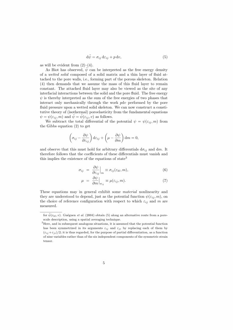
dψ = σij dεij + pdv, (5)
as will be evident from (2)–(4).As Biot has observed, ψ can be interpreted as the free energy density
of a wetted solid composed of a solid matrix and a thin layer of fluid at-tached to the pore walls, i.e., forming part of the porous skeleton. Relation(4) then demands that we assume the mass of this fluid layer to remainconstant. The attached fluid layer may also be viewed as the site of anyinterfacial interactions between the solid and the pore fluid. The free energyψ is thereby interpreted as the sum of the free energies of two phases thatinteract only mechanically through the work pdv performed by the porefluid pressure upon a wetted solid skeleton. We can now construct a consti-tutive theory of (isothermal) poroelasticity from the fundamental equationsψ = ψ(εij ,m) and ψ = ψ(εij , v) as follows.
We subtract the total differential of the potential ψ = ψ(εij ,m) fromthe Gibbs equation (2) to get(
σij −∂ψ
∂εij
)dεij +
(µ− ∂ψ
∂m
)dm = 0,
and observe that this must hold for arbitrary differentials dσij and dm. Ittherefore follows that the coefficients of these differentials must vanish andthis implies the existence of the equations of state3
σij =∂ψ
∂εij
∣∣∣m≡ σij(εkl,m), (6)
µ =∂ψ
∂m
∣∣∣σij
≡ µ(εij ,m). (7)
These equations may in general exhibit some material nonlinearity andthey are understood to depend, just as the potential function ψ(εij ,m), onthe choice of reference configuration with respect to which εij and m aremeasured.
for ψ(εkl, v). Gueguen et al. (2004) obtain (5) along an alternative route from a pore-
scale description, using a spatial averaging technique.3Here, and in subsequent analogous situations, it is assumed that the potential function
has been symmetrized in its arguments εij and εji by replacing each of them by
(εij+εji)/2; it is thus regarded, for the purpose of partial differentiation, as a function
of nine variables rather than of the six independent components of the symmetric strain
tensor.
5
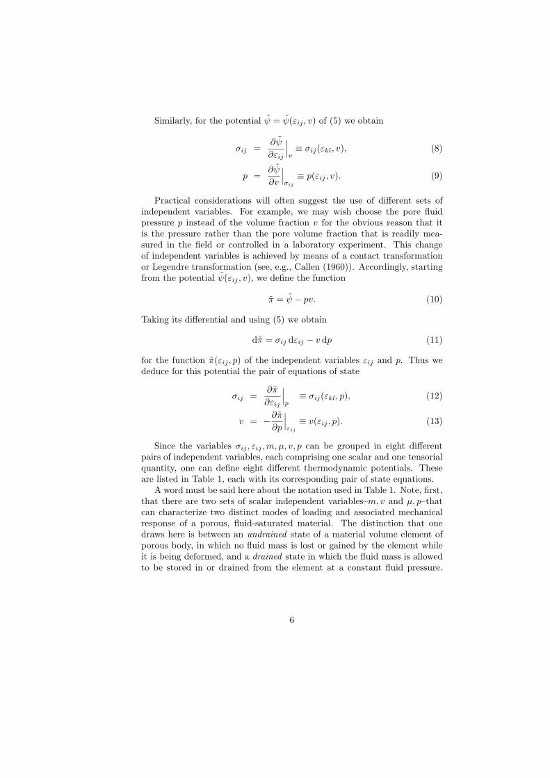
Similarly, for the potential ψ = ψ(εij , v) of (5) we obtain
σij =∂ψ
∂εij
∣∣∣v≡ σij(εkl, v), (8)
p =∂ψ
∂v
∣∣∣σij
≡ p(εij , v). (9)
Practical considerations will often suggest the use of different sets ofindependent variables. For example, we may wish choose the pore fluidpressure p instead of the volume fraction v for the obvious reason that itis the pressure rather than the pore volume fraction that is readily mea-sured in the field or controlled in a laboratory experiment. This changeof independent variables is achieved by means of a contact transformationor Legendre transformation (see, e.g., Callen (1960)). Accordingly, startingfrom the potential ψ(εij , v), we define the function
π = ψ − pv. (10)
Taking its differential and using (5) we obtain
dπ = σij dεij − v dp (11)
for the function π(εij , p) of the independent variables εij and p. Thus wededuce for this potential the pair of equations of state
σij =∂π
∂εij
∣∣∣p≡ σij(εkl, p), (12)
v = −∂π∂p
∣∣∣εij
≡ v(εij , p). (13)
Since the variables σij , εij ,m, µ, v, p can be grouped in eight differentpairs of independent variables, each comprising one scalar and one tensorialquantity, one can define eight different thermodynamic potentials. Theseare listed in Table 1, each with its corresponding pair of state equations.
A word must be said here about the notation used in Table 1. Note, first,that there are two sets of scalar independent variables–m, v and µ, p–thatcan characterize two distinct modes of loading and associated mechanicalresponse of a porous, fluid-saturated material. The distinction that onedraws here is between an undrained state of a material volume element ofporous body, in which no fluid mass is lost or gained by the element whileit is being deformed, and a drained state in which the fluid mass is allowedto be stored in or drained from the element at a constant fluid pressure.
6
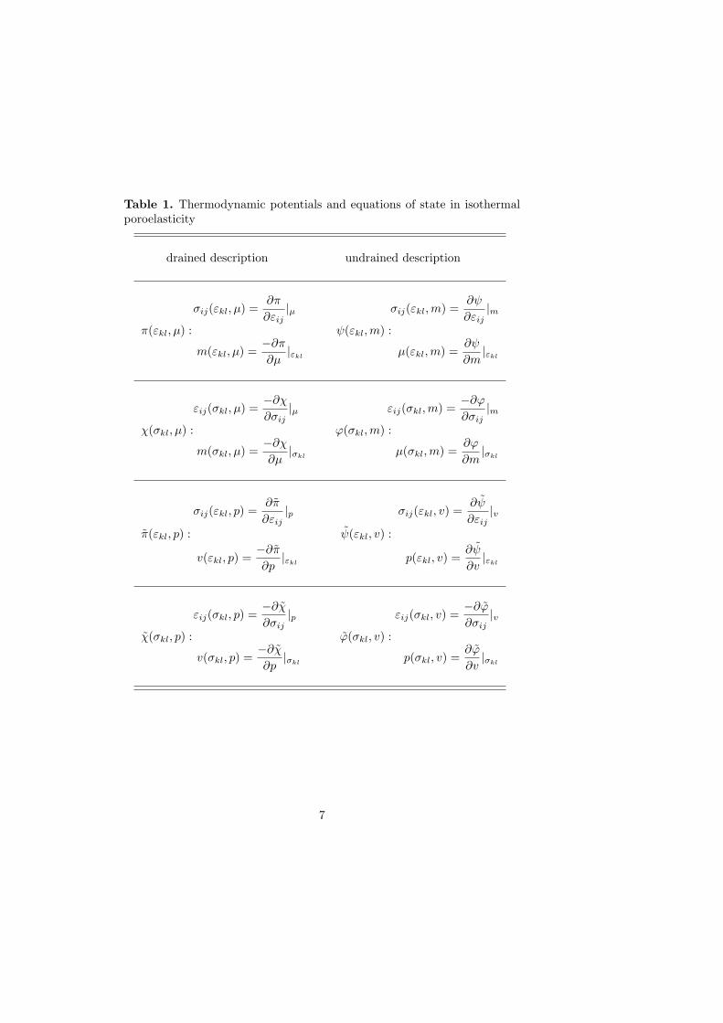
Table 1. Thermodynamic potentials and equations of state in isothermalporoelasticity
drained description undrained description
σij(εkl, µ) =∂π
∂εij|µ σij(εkl,m) =
∂ψ
∂εij|m
π(εkl, µ) : ψ(εkl,m) :
m(εkl, µ) =−∂π∂µ|εkl
µ(εkl,m) =∂ψ
∂m|εkl
εij(σkl, µ) =−∂χ∂σij
|µ εij(σkl,m) =−∂ϕ∂σij
|mχ(σkl, µ) : ϕ(σkl,m) :
m(σkl, µ) =−∂χ∂µ|σkl
µ(σkl,m) =∂ϕ
∂m|σkl
σij(εkl, p) =∂π
∂εij|p σij(εkl, v) =
∂ψ
∂εij|v
π(εkl, p) : ψ(εkl, v) :
v(εkl, p) =−∂π∂p|εkl
p(εkl, v) =∂ψ
∂v|εkl
εij(σkl, p) =−∂χ∂σij
|p εij(σkl, v) =−∂ϕ∂σij
|vχ(σkl, p) : ϕ(σkl, v) :
v(σkl, p) =−∂χ∂p|σkl
p(σkl, v) =∂ϕ
∂v|σkl
7
Since, under isothermal conditions, µ is uniquely determined by the pres-sure p, a constitutive formulation employing either p or µ as independentscalar variable will be referred to a drained description, which is to say:a description in terms of parameters obtained from experiments that wereperformed under drained conditions. On the other hand, when the fluidmass content m is held fixed in an experiment during loading, the samplewill exhibit an undrained response and this will reflect the response of boththe solid and the fluid phase. Accordingly, we shall speak of an undraineddescription, if it is phrased in terms of parameters that were obtained fromexperiments performed under undrained conditions in which either m or vwere held fixed. The case v = constant is somewhat special. Here the con-templated way of controlling the pore volume fraction in an experiment, atleast in principle, is to employ an incompressible pore fluid. For this reasonthe choice of v as an independent variable corresponds to a special case ofan undrained description.
Secondly, we shall adopt a notation that distinguishes between the ther-modynamic potentials of a fluid-saturated bulk volume element, and poten-tials that are unaffected by properties of the mobile pore fluid, i.e., charac-terize only the wetted solid skeleton of Biot. An example of the latter is thepotential ψ(εij , v) and the same superimposed tilde is used in Table 1 todenote the other three potentials for the wetted solid. Note, therefore, thatthe linear constitutive theories constructed from the four potentials listed inthe upper half of Table 1 presuppose a constant compressibility of the porefluid and for this reason will have a more restricted range of applicabilitythan their counterparts that derive from the potentials of the lower half ofthe table and which contain no reference to the equations of state of the porefluid. This difference can become important, for example in dealing with ahighly compressible pore fluid, such as natural gas, but an approximatelylinear elastic skeleton response over substantial pressure differentials. Adrained description based on the potentials π(εkl, p) or χ(σkl, p) will be theappropriate choice in such cases.
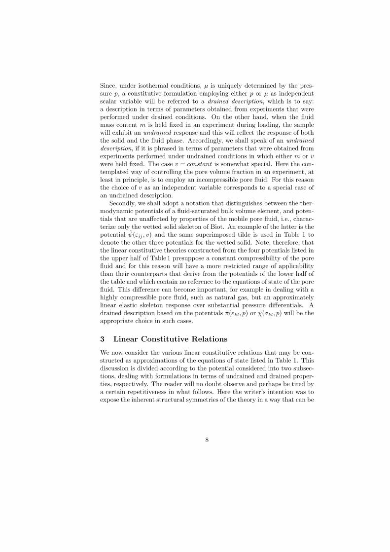
3 Linear Constitutive Relations
We now consider the various linear constitutive relations that may be con-structed as approximations of the equations of state listed in Table 1. Thisdiscussion is divided according to the potential considered into two subsec-tions, dealing with formulations in terms of undrained and drained proper-ties, respectively. The reader will no doubt observe and perhaps be tired bya certain repetitiveness in what follows. Here the writer’s intention was toexpose the inherent structural symmetries of the theory in a way that can be
8
summarized succinctly in a final table and diagram, the individual entriesof which should nevertheless remain easy to trace back to their sources ina sufficiently organized text. In the end, Table 2 and Figure 1 could thusbecome the only things to be looked at as the occasion arises.
3.1 Undrained Description
The potential ψ(εkl,m). The formal linearization procedure that weshall adopt here is to truncate a Taylor series expansion about a given refer-ence state of a set of state equations derived from a chosen thermodynamicpotential. Accordingly, in linearizing the state equations (6),(7), we specifythe reference configuration of the porous solid under consideration as onein which the strain εij vanishes throughout the body and the pore fluid hasthe density ρ0(x1, x2, x3), the volume fraction m/ρ therefore being equal tov0, and by requiring that when the body is in this state, equations (6) and(7) satisfy the relations
σ0ij = σij(0, ρ0v0) and 0 = µ(0, ρ0v0).
Here the initial stress σ0ij is understood to form an equilibrium system
of stresses in a gravitational field, satisfying the equations of equilibrium∂σ0
ij/∂xj + ρ0gi = 0, where ρ0 denotes the bulk density of the (fluid-saturated) porous solid in the reference state and gi the component of theacceleration of gravity in the direction of the coordinate xi (only rectangularCartesian coordinates are considered).
In expanding (6) & (7), we continue to assume small displacement gra-dients. In addition, so as to obtain a fully linear undrained description, weshall permit only such changes in fluid mass content as will be compati-ble with the assumption of a constant fluid compressibility. We shall seepresently, however, that linear poroelasticity is not contingent upon this lastassumption.
The linear approximations of (6) & (7) thus become
σij(εkl,m0 + ∆m;R) = σij |0 +∂σij∂εkl
∣∣∣0mεkl +
∂σij∂m
∣∣∣0εkl
∆m
andµ(εij ,m0 + ∆m) = µ|0 +
∂µ
∂εij
∣∣∣0mεij +
∂µ
∂m
∣∣∣0εij
∆m,
where the superscript ‘0’ denotes evaluation at the reference state, σij |0 =σ0ij denotes the initial stress as specified above, and µ|0 = 0. We now
express these linear relationships in the form
σij = σ0ij + Cuijkl εkl − aij∆m/ρ0, (14)
9
andµ = −ρ−1
0 aij εij + ρ−10 Mε∆m/ρ0, (15)
by defining the following constant coefficients: The rank-4 tensor of undrainedelastic constants or undrained stiffnesses with components
Cuijkl =∂σij∂εkl
∣∣∣0m
=∂2ψ
∂εkl∂εij
∣∣∣0, (16)
a rank-2 tensor with components
aij = −ρ0∂σij∂m
∣∣∣0εkl
= −ρ0∂2ψ
∂m∂εij
∣∣∣0
= −ρ0∂µ
∂εij
∣∣∣0m, (17)
expressing the change in stress with fluid mass content when the strain isheld fixed and equal to zero (or the change in the pressure function withstrain when the mass content is held fixed), and the scalar
ρ−10 Mε = ρ0
∂µ
∂m
∣∣∣0εij
= ρ0∂2ψ
∂m2
∣∣∣0. (18)
Note the appearance of the same coefficient aij in both (14) and (15),which is implied by a Maxwell-type reciprocity relation that derives fromthe interchangeability of the order of differentiation in the mixed derivativesof the potential ψ in (17).
It is not difficult to see, that a change in fluid mass content at constantstrain will, in general, evoke a non-hydrostatic stress response and that thisdemands a tensorial coefficient aij . One only has to think of a porosity thatis at least partly due to the presence of low-aspect ratio, crack-like poresthat display a certain measure of preferred orientation.
A straightforward interpretation of the coefficient Mε will be given fur-ther below in terms of its reciprocal 1/Mε, which has the significance ofa specific storage capacity at constant strain. We note here that Mε isidentical with the modulus M of Biot and Willis (1957). In the presentcontext the subscript ‘ε’ serves to distinguish Mε from a similar modulusMσ (cf. Eq. 26) that is defined at constant stress rather than strain.
The symmetry of εij and σij implies the symmetries of aij and Cuijklwith respect to the interchanges i ↔ j and k ↔ l of indices, and a furthersymmetry of Cuijkl with respect to the pairwise interchange ij ↔ kl followsfrom the interchangeability in (16) of the order of differentiation of thepotential function ψ(εkl,m) with respect to the strain components. Thesymmetries
aij = aji and Cuijkl = Cujikl = Cuijlk = Cuklij (19)
10
must therefore apply, so that there are at most 6 independent components ofaij and 21 independent components of Cuijkl. These numbers will be reducedfor any a particular poroelastic material by further, material symmetries.
The potential ϕ(σkl,m). Consider the set of state equations
εij = − ∂ϕ
∂σij
∣∣m≡ εij(σkl,m) (20)
µ =∂ϕ
∂m
∣∣εij≡ µ(σkl,m) (21)
that derives from the potential ϕ(σkl,m) = ψ(εkl,m)− σijεij . We linearizethese equations about a reference state in which σkl = σ0
kl and m = ρ0v0,and in which (22) & (21) satisfy the conditions
0 = εij(σ0kl, ρ0v0) and µ0 = µ(σ0
kl, ρ0v0).
With ∆m = m− ρ0v0 the resulting linear constitutive relations are
εij = Suijkl (σkl − σ0kl) + bij ∆m/ρ0, (22)
andµ = −ρ−1
0 bij (σij − σ0ij) + ρ−1
0 Mσ∆m/ρ0. (23)
The constant coefficients in (22) and (23) are the components of therank-4 tensor of undrained elastic compliances
Suijkl =∂εij∂σkl
∣∣∣0m
= − ∂2ϕ
∂σkl∂σij
∣∣∣0, (24)
the components of a symmetric rank-2 tensor
bij = ρ0∂εij∂m
∣∣∣0σkl
= −ρ0∂2ϕ
∂m∂σij
∣∣∣0
= −ρ0∂µ
∂σij
∣∣∣m, (25)
expressing the change in strain with fluid mass content when the stressesare held fixed at their initial values (or the change in the pressure functionwith stress when the mass content is held fixed), and the scalar
ρ−10 Mσ = ρ0
∂µ
∂m
∣∣∣0σij
= ρ0∂2ϕ
∂m2
∣∣∣0, (26)
which we shall interpret presently through its reciprocal 1/Mσ.We note here that coefficient defined by (25) is the same as Thompson
and Willis (1991) coefficient bij ; it represents, as we shall see, an appro-priate generalization of Skempton’s scalar pore pressure coefficient B, such
11
that bij = bδij = 13Bδij for an isotropic medium. The appearance of this
coefficient in both (22) and (23) is implied by a Maxwell-type reciprocity re-lation that derives from the interchangeability of the order of differentiationin the mixed derivatives of the potential ϕ in (25).
Two comments are now in order. The first applies to each of the variousrenderings in this section of the linear theory. It is the observation that thecoefficients Cuijkl, aij ,Mε and Suijkl, bij ,Mσ may be interpreted as specifyingtangent directions in εij ,m- respectively σij ,m-space at the reference state,on which they depend. The linearization procedure we have just describedis therefore general enough to allow for an incrementally linear descriptionnear any suitably selected reference state.
Secondly, Cuijkl and Suijkl were referred to as undrained coefficients, be-cause they are defined in terms of partial derivatives taken at fixed fluidmass content. This terminology does not imply, however, that the use ofthese constants is restricted to conditions of constant fluid mass content,although it will be a natural choice in such circumstances.4
The potential ψ(εkl, v). The choice of this potential, which satisfiesthe Gibbs equation (5), is primarily of theoretical interest, since the stateequations (8) & (9) are linearized in this case in the displacement gradientand in the change in volume fraction, i.e., in the two kinematic variables.Although the volume fraction v remains an impractical choice of indepen-dent variable, the condition |∆v| = |v − v0| � 1 represents nonetheless themost appropriate among the constraints that may be imposed on the var-ious possible scalar independent variables. For while it is consistent withthe idea of infinitesimal elastic deformations of the solid skeleton materialof a porous body, it imposes no direct constraint on the magnitude of porepressure changes. This also explains why Biot (1941) chose to develop histheory from the potential ψ(εkl, v).
A reference configuration is now defined for the porous body under con-sideration such that the strain εij vanishes and that its pore volume fractionequals v0(x1, x2, x3) in this configuration, while equations (8) and (9) satisfy
σ0ij = σij(0, v0) and p0 = p(0, v0).
A truncated Taylor series expansion of (8) & (9) now yields the linear
4An undrained response may be expected, for example, for the propagation of low-
frequency (ω) seismic waves, where the relaxation time for pore pressure diffusion
(which is proportional to the square of the distance between rarefied and compressed
regions over which fluid transport must take place) is large in comparison with 1/ω.
12
constitutive relations
σij = σ0ij + Cuijkl εkl − aij∆v. (27)
andp = p0 − aij εij + Mε∆v, (28)
Here
Cuijkl =∂σij∂εkl
∣∣∣0v
=∂2ψ
∂εkl∂εij
∣∣∣0
(29)
are the components of a rank-4 tensor of undrained elastic constants orstiffnesses, pertaining to the special case of an incompressible pore fluid,
aij = −∂σij∂v
∣∣∣0εkl
= − ∂2ψ
∂v∂εij
∣∣∣0
= − ∂p
∂εij
∣∣∣0v
(30)
are the components of a symmetric rank-2 tensor that expresses the changein stress with the pore volume fraction when the strain is held fixed andequal to zero (or the change in pore pressure when the pore volume fraction–or incompressible fluid mass content–is held fixed), and
Mε =∂p
∂v
∣∣∣0εij
=∂2ψ
∂v2
∣∣∣0. (31)
Note again the appearance of the same coefficient aij in both (27) and (28),which is implied by a Maxwell-type reciprocity relation that derives fromthe interchangeability of the order of differentiation in the mixed derivativesof the potential ψ in (30). This enables us to identify the volume fractioncoefficient in (27) with the strain coefficient in (28) and allows us to interpretSuijkl and aij as coefficients pertaining to an undrained description, albeitone of a special kind for which the fluid density remains constant and equalto ρ0.
The potential ϕ(σkl, v). As a last set of state equations providing anundrained description, we consider the pair
εij = − ∂ϕ
∂σij
∣∣∣0v≡ εij(σkl, v), (32)
p =∂ϕ
∂v
∣∣∣0εij
≡ p(σkl, v), (33)
which can be derived from the potential ϕ(σkl, v) = ψ(εkl, v)− σijεij . Lin-earizing about a reference state in which σkl = σ0
kl and v = v0, and in which(32) & (33) satisfy the conditions
0 = εij(σ0kl, v0) and p0 = p(σ0
kl, v0),
13
we obtainεij = Suijkl (σkl − σ0
kl) + bij ∆v, (34)
andp = p0 − bij (σij − σ0
ij) + Mσ∆v. (35)
Here
Suijkl =∂εij∂σkl
∣∣∣0v
= − ∂2ϕ
∂σkl∂σij
∣∣∣0
(36)
denote the components of the tensor of undrained elastic compliances,
bij =∂εij∂v
∣∣∣0σkl
= − ∂2ϕ
∂v∂σij
∣∣∣0
= − ∂p
∂σij
∣∣∣0v
(37)
expresses the change in strain with the pore volume fraction when thestresses are held fixed at their initial values (or the change in pore pres-sure with stress when the volume fraction is held fixed it its initial value),and
Mσ =∂p
∂v
∣∣∣0σij
=∂2ϕ
∂v2
∣∣∣0. (38)
The appearance of the same coefficient bij in both (34) and (35) is impliedby the reciprocity relation expressed in (37). This enables us to identifythe volume fraction coefficient in (27) with the strain coefficient in (28)and allows us to interpret both, Cuijkl and bij as coefficients pertaining toa special undrained description in which the pore fluid is assumed to beincompressible.
Relationships between undrained coefficients. From (16) and (24)it follows by an application of the chain rule that
Suijkl Cuklmn =
∂εij∂σkl
∣∣∣0m
∂σkl∂εmn
∣∣∣0m
=12
(δimδjn + δinδjm) . (39)
Making use of this result in (14), after multiplication by Suijkl, we get
Suijkl Cuklmn εmn = εij = Suijkl(σkl − σ0
kl) + Suijkl akl∆m/ρ0
and, upon comparing this with (22),
bij = Suijkl akl. (40)
Similarly, one finds that
Cuijkl Suklmn =
12
(δimδjn + δinδjm) . (41)
14
Using this property in (22), after multiplication by Cuijkl, gives
σij − σ0ij = Cuijkl εkl − Cuijkl bkl∆m/ρ0
and, upon comparing this with (14),
aij = Cuijkl bkl. (42)
Further, it is seen from (15) and (23) that
(Mσ −Mε)∆m/ρ0 = bij(σij − σ0ij)− aijεij ,
hence it follows from (14), (40) and (42) that
Mε −Mσ = aij bij = aij Suijkl akl = bij C
uijkl bkl. (43)
The same relationships evidently exist among the coefficients that aredistinguished by a tilde as pertaining to an undrained description for in-compressible pore fluids.
3.2 Drained Description
The potential π(εkl, p). The equations of state (12) & (13) associatedwith this potential are linearized about a reference state in which the strainεij vanishes and by demanding that they satisfy
σ0ij = σij(0, p0) and v0 = v(0, p0).
when the pore pressure equals p0(x1, x2, x3) throughout a given porousbody.
In truncating the series expansion (12) & (13) about this reference stateafter the linear terms, we shall as usual assume all components of displace-ment gradient to remain much smaller than one. Note, however, that weneed not impose the same constraint on the relative change in pore pressure.The only constraint that we impose on pore pressure changes is that theyremain consistent with the kinematic assumption of small changes in thepore volume fraction. The resulting linear constitutive relations are nowwritten
σij = σ0ij + Cijkl εkl − αij∆p (44)
andv = v0 + αij εij + Sε∆p, (45)
with the drained stiffnesses
Cijkl =∂σij∂εkl
∣∣∣0p
=∂2π
∂εkl∂εij
∣∣∣0, (46)
15
the pore pressure coefficient or Biot coefficient
αij = −∂σij∂p
∣∣∣0εkl
= − ∂2π
∂p∂εij
∣∣∣0
=∂v
∂εij
∣∣∣0p, (47)
and the specific storage capacity or specific storage coefficient at constantstrain5
Sε =∂v
∂p
∣∣∣0εij
= −∂2π
∂p2
∣∣∣0. (48)
We recall here that in Biot (1941) the change ∆v in the void volumefraction is denoted by θ; also, the coefficients αij and Sε correspond toBiot’s αδij and Q−1, respectively, for isotropic porous media.
An immediate consequence of (44) is that the quantity
∆σ′ij = σij − σ0ij + αij ∆p (49)
furnishes an appropriate generalization for anisotropic poroelastic materialsof the familiar Biot-Willis effective stress (Biot and Willis, 1957; Geertsma,1957b; Nur and Byerlee, 1971). The existence of an effective stress principlein poroelasticity is in fact a necessary consequence of linearization alone andis contingent upon no additional requirements. It is independent, in partic-ular, of micro-mechanical properties other than the elastic skeleton responseimplied by the above formulation based on work potentials, although it iswell known (Nur and Byerlee, 1971; Carroll, 1979) that the coefficient αijis more directly related to the pore-scale elastic constants of the solid phasewhen these remain uniform throughout a representative elementary volumeof the porous medium (see the discussion further below). However, inde-pendent of any micro-mechanical interpretation, the coefficient αij retainsthe straightforward significance given to it by (47) of a quantity that canbe determined directly from suitable macroscopic experiments.
We note further that since the potentials π and ψ are related by thecontact transformation π = ψ − pv, the pair (44),(45) of linear consti-tutive relations could in fact have been obtained directly by rearranging(27),(28) so as to resemble (44),(45) in form, and by determining the coef-ficients Cijkl, αij , Sε in terms of the given coefficients Cuijkl, aij , Mε. Thus,by rewriting (28) as
∆v =1Mε
aklεkl +1Mε
∆p
5We consider storage capacity more telling than the customary storage coefficient ; it
is also suggestive of the scalar nature of this quantity. The qualification ‘specific’ is
commonly understood to mean ‘per unit mass’, but a specific storage capacity can
obviously express a capacity to store so many kg per kg per unit pressure change or
so many m3 per m3 per unit pressure change.
16
and substituting this expression for ∆v in (27), we obtain
σij = σ0ij + (Cuijkl −
1Mε
aij akl)εkl −1Mε
aij∆p.
Therefore the following relationships between the coefficients of the formu-lations (44),(45) and (27),(28) must hold:
Cijkl = Cuijkl −1Mε
aij akl, αij =1Mε
aij , Sε =1Mε
. (50)
These provide a first set of relationships between the coefficients of a drainedand those of an undrained description, albeit for the special case of anincompressible pore fluid.
The potential χ(σkl, p). Observing that χ(σkl, p) = π(εkl, p)− σijεijis obtained by a contact transformation from the previous potential, weavoid further repetition and write down the linear constitutive relations
εij = Sijkl (σkl − σ0kl) + βij ∆p (51)
andv = v0 + βij (σij − σ0
ij) + Sσ∆p, (52)
where
Sijkl =∂εij∂σkl
∣∣∣0p
= − ∂2χ
∂σkl∂σij
∣∣∣0
(53)
are the drained elastic compliances,
βij =∂εij∂p
∣∣∣0σkl
= − ∂2χ
∂p∂σij
∣∣∣0
=∂v
∂σij
∣∣∣0p
(54)
are the components of a symmetric hydraulic expansion tensor, and
Sσ =∂v
∂p
∣∣∣0σij
= −∂2χ
∂p2
∣∣∣0
(55)
is a hydraulic void expansion coefficient at constant stress.We note here that the parameter H−1 in Biot’s 1941 paper represents
the equivalent of the trace 3β of the tensor βij for the case of isotropy, whileBiot’s parameter R−1 is our Sσ.
From (52) it is apparent that the pore volume change is controlled bythe effective stress quantity
σij − σ0ij + Sσβ
−1ij ∆p (56)
17
where β−1ij is the inverse of βij .
The coefficients αij , Cijkl and βij , Sijkl are referred to as drained co-efficients, because they are defined in terms of partial derivatives taken atfixed pore pressure. This terminology does not imply, however, that theuse of these constants is restricted to conditions of constant pore pressure.Indeed, the full description of any poroelastic process may always be cast interms of the variable sets σij , p or εij , p. The drained constants are of coursethe natural choice for the description of drained processes, i.e., poroelasticprocesses in which the pressure appears merely in the role of a constantparameter.
We note further that since the potentials χ and ϕ are related by thecontact transformation χ = ϕ − pv, the pair (51),(52) of linear consti-tutive relations could in fact have been obtained directly by rearranging(34),(35) so as to resemble (51),(52) in form, and by determining the coef-ficients Sijkl, βij , Sσ in terms of the given coefficients Suijkl, bij , Mσ. Thus,by rewriting (35) as
∆v =1Mσ
bklεkl +1Mσ
∆p
and substituting this expression for ∆v in (34), we obtain
σij = σ0ij + (Suijkl −
1Mσ
bij bkl)εkl −1Mσ
bij∆p.
From these we deduce the following relationships between the coefficientsof the formulations (51),(52) and (34),(35)
Sijkl = Suijkl −1Mσ
bij bkl, βij =1Mσ
bij , Sσ =1Mσ
. (57)
This represents a second set of relationships between the coefficients of adrained and those of an undrained description for the special case of anincompressible pore fluid.
The potential π(εkl, µ). An alternative drained description, based onthe potential π(εkl, µ) = ψ(εkl,m)−µm, is obtained directly upon rewritingthe linear relationships (14),(15) in terms of the independent varible µ. Sincethe latter is a unique function of the pressure p, this will indeed correspondto another drained description6. Thus we write
σij = σ0ij + Cijklεkl − αijρ0µ, (58)
6Note, however, that the present description will involve the assumption of a constant
fluid compressibility, which is why the above linear drained descriptions based on the
potentials π(εkl, p) and χ(σkl, p) are the preferred ones for highly compressible pore
fluids.
18
and∆m/ρ0 = αij εij + Sερ0µ, (59)
observing that the stiffness tensor must be the same as in (44), and that
αij = − 1ρ0
∂σij∂µ
∣∣∣0εkl
= − 1ρ0
∂2π
∂µ∂εij
∣∣∣0
=1ρ0
∂m
∂εij
∣∣∣0µ
= −∂σij∂µ
dµdp
∣∣∣0εkl
= −∂σij∂p
∣∣∣0εkl
,
the latter on account of (47). Further, in the linearised theory under con-sideration, the change in fluid mass content per unit reference volume maybe written in terms of the changes in fluid density and void volume fractionas
∆m = m−m0 = ρ0(v − v0) + (ρ− ρ0)v0, (60)
so that one has
1ρ0
∂m
∂p
∣∣∣0εkl
=1ρ0
∂m
∂µ
dµdp
∣∣∣0εkl
=∂v
∂p
∣∣∣0εkl
+ v01ρ0
∂ρ
∂p
∣∣∣0,
that isSε = Sε + v0cf , (61)
where cf = (1/ρ0)(∂ρ/∂p)|0 = (ρ − ρ0)/ρ0∆p is a constant compressibilityof the fluid for the small changes in the fluid density implied by (60).
We return here for a moment to relation (45), adding a term (ρ −ρ0)v0/ρ0 = v0cf∆p on both sides to note that the result can be written∆m/ρ0 = αij εij + (Sε + v0cf )∆p. Evidently, therefore, the independentvariable ρ0µ may be replaced by the pore pressure change ∆p in the aboveconstitutive relations (58),(59), so that we recover (44) together with
∆m/ρ0 = αij εij + Sε∆p. (62)
as an alternative set of constitutive relations. From this Sε is seen to havethe simple interpretation of a specific storage capacity at fixed strain andthis also explains the nature of its reciprocal Mε.
Putting now (15) into the form
∆m/ρ0 =1Mε
akl εkl +1Mε
ρ0µ
and introducing this in (14), we find
σij = σ0ij + (Cuijkl −
1Mε
aijakl)εkl −1Mε
aijρ0µ.
19
A comparison with (58),(59) or (44),(62) then shows that the coefficients inthese descriptions are related to those of the undrained description (14),(15)by
Cijkl = Cuijkl −1Mε
aijakl, αij =1Mε
aij , Sε = Sε + v0cf =1Mε
. (63)
In particular, the relationship between the drained and the undrained stiff-nesses may be expressed in the following ways
Cuijkl − Cijkl = αijakl = Mεαijαkl = Sεaijakl. (64)
The same relationship between Cuijkl and Cijkl, expressed in terms ofMε and αij was recorded earlier by Rudnicki (1985). It is of course ananticipated result, bearing in mind the formally analogous relations thatexist in thermoelasticity between isothermal and adiabatic moduli7.
Note also that the relations (63) will reduce to (50), as they must, if thefluid compressibility vanishes.
The potential χ(σkl, µ). Finally, a further alternative drained de-scription, based on the potential χ(σkl, µ) = ϕ(σkl,m) − µm, is obtainedby rewriting the linear relationships (22),(23) in terms of the independentvarible µ as
εij = Sijkl(σkl − σ0kl) + βijρ0µ, (65)
and∆m/ρ0 = βij(σij − σ0
ij) + Sσρ0µ, (66)
observing that the compliance tensor must be the same as in (51), and that
∂εij∂p
∣∣∣0σkl
=∂εij∂µ
dµdp
∣∣∣0σkl
=1ρ0
∂εij∂µ
∣∣∣0σkl
= βij
on account of (54). Assuming, as before, that the change in fluid masscontent per unit reference volume can be approximated by (60), one has
1ρ0
∂m
∂p
∣∣∣0σkl
=1ρ0
∂m
∂µ
dµdp
∣∣∣0σkl
=∂v
∂p
∣∣∣0σkl
+ v01ρ0
∂ρ
∂p
∣∣∣0,
that isSσ = Sσ + v0cf , (67)
from which it is apparent that Sσ represents a specific storage capacityat constant stress. This interpretation of Sσ also clarifies the nature of
7Excellent discussions may be found in Nye (1957) and in Weiner (1983).
20
its reciprocal Mσ. We note further that Sσ is identical with the “storagecompressibility” S of Kumpel (1991).
Again, we find that the constitutive relations (65),(66) may be cast al-ternatively in terms of the pore pressure change, yielding (51) and
∆m/ρ0 = βij(σij − σ0ij) + Sσ∆p. (68)
as an alternative set.We now put (23) into the form
∆m/ρ0 =1Mσ
bkl(σkl − σ0kl) +
1Mσ
ρ0µ
and introduce this in (22) to obtain
εij = (Suijkl −1Mσ
bijbkl)(σkl − σ0kl)−
1Mσ
bijρ0µ.
The coefficients of the drained descriptions (65),(66) or (51),(68) and theundrained description (22),(23) are therefore related by
Sijkl = Suijkl −1Mσ
bijbkl, βij =1Mσ
bij , Sσ = Sσ + v0cf =1Mσ
. (69)
In particular, the relationship between the drained und the undrained com-pliances may be expressed in the following ways
Sijkl − Suijkl = βijbkl = Mσβijβkl = Sσbijbkl. (70)
Note that the relations (69) reduce to (57), as they must, if the fluidcompressibility vanishes.
A further observation, concerning equation (68), is that the quantity
σij − σ0ij + Sσβ
−1ij ∆p (71)
plays the role of an effective stress governing the change in fluid mass content(here β−1
ij denotes the inverse of βij). For isotropic materials, Sσ/β−1ij =
b−1ij = b−1δij = (3/B)δij , so that in this case (68) takes the form
∆m/ρ0 = β
(σkk − σ0
kk +3B
∆p)
(72)
in terms of Skempton’s coefficient B, which is thus seen to govern the porepressure response to changes in mean stress under undrained conditions
∆p = −Bσkk − σ0kk
3. (73)
21
As was shown by Rice and Cleary (1976), the fluid mass content (72) ofa slightly compressible fluid satisfies the homogeneous diffusion equation8
c∇2m = ∂m/∂t, (74)
in which c is a coefficient of consolidation or hydraulic diffusivity that isgiven by (cf. Eq. 17 in Rice and Cleary (1976))
c =k
η
[2GB2(1 + νu)2(1− ν)
9(1− νu)(νu − ν)
], (75)
and where k is the absolute permeability9 of the (isotropic) medium (in m2)and η is the viscosity of its pore fluid (in Pa s). Also, ν and νu denote thedrained and undrained Poisson ratio, respectively, as defined and discussedfurther below. Making use of the relationships given there for isotropicmaterials and the above definitions of the storage parameters Sσ and Sε, itis easily seen that the hydraulic diffusivity can be defined alternatively bythe following expressions in terms of the parameters α, β, ν and Sσ or Sε(see Eqs. 112–117 further below)
c =k/η
Sσ − [2(1− 2ν)/(1− ν)]αβ=
k/η
Sε + [(1 + ν)/(1− ν)]αβ. (76)
The quantity in brackets in (75) thus represents the reciprocal of
S = Sσ − [2(1− 2ν)/(1− ν)]αβ = Sε + [(1 + ν)/(1− ν)]αβ, (77)
which provides two of several equivalent expressions for a specific storagecapacity or storage coefficient10. Note, however, that elsewhere in the litera-ture the symbol S is often used to denote a different storage parameter (see,e.g., Wang (2000). Also, Green and Wang (1990) define a specific storagecoefficient Ss = ρfgS as the product of (77) and the unit weight of water.
8Note that (74) becomes a rigorous result for incompressible pore fluids, when in effect
it reduces to a diffusion equation for the change ∆v in pore volume fraction.9In order to avoid any confusion with the elastic bulk modulus K, we denote the absolute
permeability by the lower-case symbol k; we thereby depart from the standard notation
K in the hydrological literature, where the lower-case letter is usually reserved for the
so-called coefficient of permeability k = ρgK/η with the dimension of a velocity; ρ and
η then denote the uniformly constant density and viscosity of the groundwater.10See also Jaeger et al. (2007, chap. 7) on this point.
22
Relationships between drained coefficients. From (46) and (53) itfollows by an application of the chain rule that
Sijkl Cklmn =∂εij∂σkl
∣∣∣0p
∂σkl∂εmn
∣∣∣0p
=12
(δimδjn + δinδjm) . (78)
Substitution of this result in (44) also yields
Sijkl Cklmn εmn = εij = Sijkl(σkl − σ0ijkl) + Sijkl αkl∆p
and, upon comparing this with (51),
βij = Sijkl αkl. (79)
In particular, if the porous medium is isotropic, its response is characterizedby the isotropic tensors αij = αδij , βij = βδij and Sijkl = 1
4G (δikδjl +δilδjk) + ( 1
9K −1
6G )δijδkl, where K is the drained bulk modulus and G isthe shear modulus of the of the porous solid. The last relation thereforereduces to (cf. Biot (1941), Eq. 2.11)
β =13Siikk α =
α
3K. (80)
Similarly, one finds that
Cijkl Sklmn =12
(δimδjn + δinδjm) (81)
Using this property in (51), after multiplication by Cijkl, gives
σij − σ0ij = Cijkl εkl − Cijkl βkl∆p
and, upon comparing this with (44),
αij = Cijkl βkl. (82)
In the case of isotropy, with Cijkl = G(δikδjl + δilδjk) + (K − 2G/3)δijδkland Ciikk = 9K, this again reduces to (80).
From (44),(45), and (82), it also follows that
v − v0 = Cijkl βkl εij + Sε∆p = βij(σij − σ0ij) + (αijβij + Sε)∆p
and hence, from (52),(61),(67),(79), and (82),
Sσ − Sε = Sσ − Sε = αij βij = αij Sijkl αkl = βij Cijkl βkl. (83)
For an isotropic porous medium one obtains (cf. Biot (1941), Eq. 2.12)
Sσ − Sε = Sσ − Sε = 3αβ = K−1α2 = 9Kβ2. (84)
23
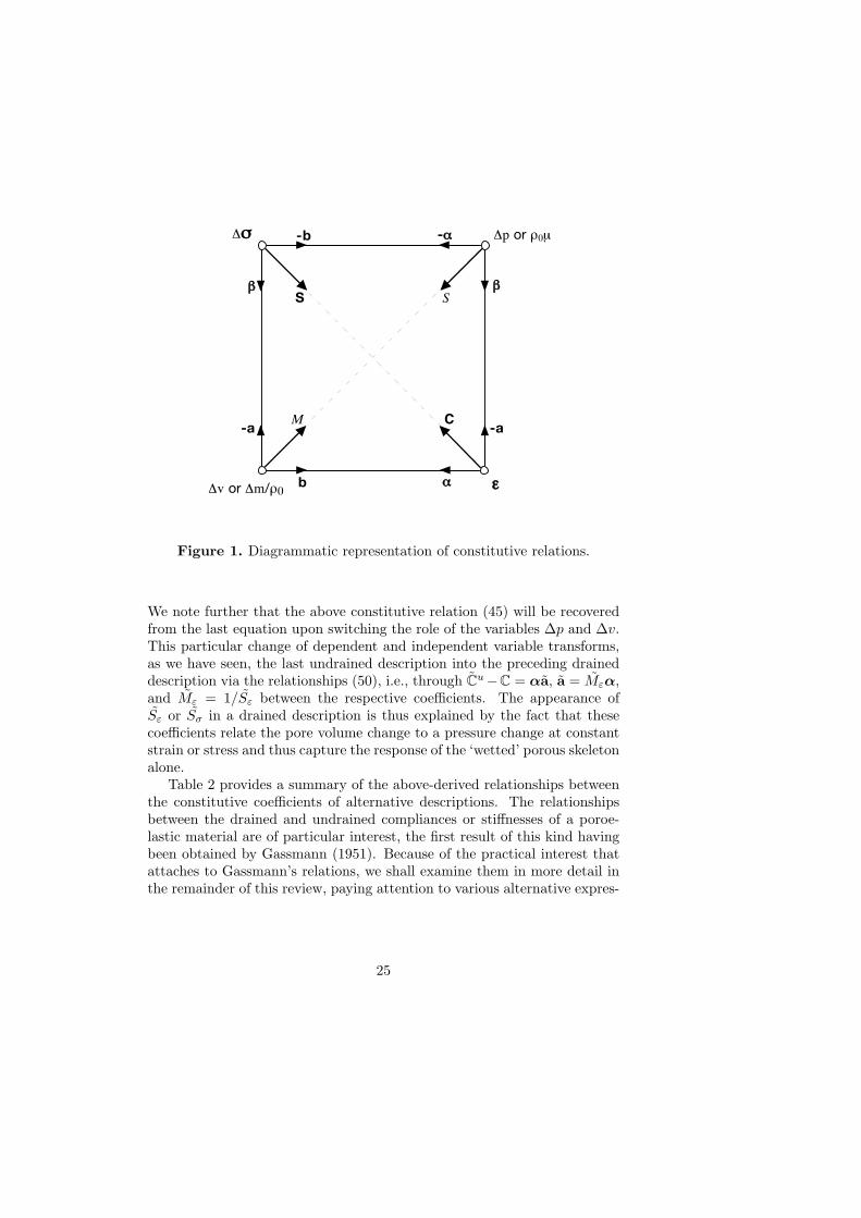
3.3 Diagrammatic Representation of Constitutive Relations; Sum-mary of Relationships Between Constitutive Coefficients
The entire set of linear constitutive relations derived in the above canbe displayed in the form of a diagram by positioning the two tensorial fieldvariables ∆σij and εij and the two pairs of (alternative) scalar field variables∆p, ρ0µ and ∆v,∆m/ρ0 at diagonally opposite corners of a square (Fig. 1).Every pair of constitutive relations comprises one tensor- and one scalar-valued equation in one tensorial and one scalar independent variable, as forexample the set formed by (44) & (45), which we may write
∆σ = C : ε−α∆p,∆v = α : ε+ Sε∆p,
in direct tensor notation11. These equations are extracted from Figure 1 byselecting the pair of dependent variables ∆σ,∆v and the pair of independentvariables ε,∆p and by factoring the latter with the coefficients C,α, Sε thatlabel the arrows pointing from the independent to the dependent variablealong a connecting line.
Here the following rules must be observed: A subscript ε or σ must beattached to the scalar coefficient S and its reciprocal M = 1/S in all cases asan indication of the chosen independent tensorial variable. If ∆p or ρ0µ areselected as dependent variables, the rank-4 tensors C or S are to be viewedas drained coefficients and these carry no superscript. On the other hand,if ∆m/ρ0 or ∆v are selected as dependent variables, then the undrainedcoefficients Cu or Su apply. Accordingly, for example, one recovers (22) &(23)
ε = Su : ∆σ + b ∆m/ρ0,
ρ0µ = −b : ∆σ +Mσ∆m/ρ0,
upon selecting ∆σ and ∆m/ρ0 as independent variables. However, choosing∆v as independent variable will require a tilde to be placed upon all coeffi-cients for such special undrained descriptions, yielding for example (27) &(28)
∆σ = Cu : ε− a ∆v,∆p = −a : ε+ Mε∆v.
11Here the double-dot product α : ε = αijεij denotes the scalar product of two rank-2
tensors, C : ε the double contraction of rank-4 tensor C with rank-2 tensor ε giving the
rank-2 tensor with components Cijklεkl.
24
S
C
-b
-a
β
-αΔσ
βS
αb
-a
εΔv or Δm/ρ0
Δp or ρ0µ
M
Figure 1. Diagrammatic representation of constitutive relations.
We note further that the above constitutive relation (45) will be recoveredfrom the last equation upon switching the role of the variables ∆p and ∆v.This particular change of dependent and independent variable transforms,as we have seen, the last undrained description into the preceding draineddescription via the relationships (50), i.e., through Cu−C = αa, a = Mεα,and Mε = 1/Sε between the respective coefficients. The appearance ofSε or Sσ in a drained description is thus explained by the fact that thesecoefficients relate the pore volume change to a pressure change at constantstrain or stress and thus capture the response of the ‘wetted’ porous skeletonalone.
Table 2 provides a summary of the above-derived relationships betweenthe constitutive coefficients of alternative descriptions. The relationshipsbetween the drained and undrained compliances or stiffnesses of a poroe-lastic material are of particular interest, the first result of this kind havingbeen obtained by Gassmann (1951). Because of the practical interest thatattaches to Gassmann’s relations, we shall examine them in more detail inthe remainder of this review, paying attention to various alternative expres-
25
sions in terms of particular set of material parameters that can be obtainedfrom so-called unjacketed tests.
The pair-structure of the constitutive theory of poroelasticity, compris-ing one tensorial and one scalar relation and three constitutive coefficients ofdifferent tensorial rank, is not always brought out clearly in the literature.Thompson and Willis (1991), for example, derive a relationship for ∆m/ρ0
(their equation 32), in which the coefficient of the pore fluid pressure be-comes Sjjklαkl/bii − αijSijklαkl. But this is simply an expression for thescalar coefficient Sε, as is easily seen from the relationships listed in Table 2,so that their equation 32 is the same as (62); its existence could thus havebeen inferred directly from the relevant thermodynamic potential π(εkl, µ).
Table 2 and Figure 1 provide readers with a summary of the informationneeded to gain a rapid overview over the various possible alternative for-mulations of linear poroelasticity. As has been emphasized in the aboveat various places, the fundamental choice that one faces in practice is be-tween a formulation in terms of the properties of Biot’s “wetted solid” anda formulation that will include properties of the pore fluid, viz. a constantfluid compressibility, in the constitutive description. Looking again at Ta-ble 1 one would, after all that has been said in the above, most likely comeup with a choice of either a drained description based on the potentialsπ(εkl, p) or χ(σkl, p) or an undrained description based on the potentialsψ(εkl,m) or φ(σkl,m). As a linear theory, the latter would demand a con-stant fluid compressibility, as we have seen. If one wished to preserve thelinear elastic response of a wetted porous solid, but at the same time allowfor the presence of a highly compressible fluid phase and large changes influid pressure, then a drained description will be the appropriate choice,since it allows us to defer any account of fluid behaviour to the formulationof the final field equations of the theory. An undrained description in termsthe potential ψ(εkl, v) would offer the same advantage, were it not for theimpractical choice of the volume fraction as independent variable. The po-tential ψ(εkl, v) nevertheless furnishes the appropriate point of departure inconstructing a linear theory, as we have seen. It was selected by Biot (1941)for this purpose. Biot however rewrote the resulting constitutive relationsin terms of the stress and the pore pressure as independent variables, whichamounts to writing the (isotropic) equivalent of our Eqs. (51),(52) ratherthan (34),(35).
26
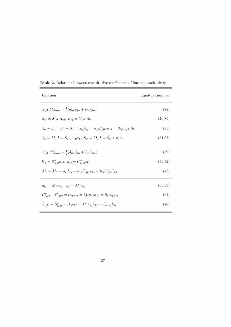
Table 2. Relations between constitutive coefficients of linear poroelasticity
Relation Equation number
SijklCklmn = 12 (δimδjn + δinδjm) (78)
βij = Sijklαkl, αij = Cijklβkl (79,82)
Sσ − Sε = Sσ − Sε = αijβij = αijSijklαkl = βijCijklβkl (83)
Sε = M−1ε = Sε + v0cf , Sσ = M−1
σ = Sσ + v0cf (61,67)
SuijklCuklmn = 1
2 (δimδjn + δinδjm) (39)
bij = Suijklakl, aij = Cuijklbkl (40,42)
Mε −Mσ = aijbij = aijSuijklakl = bijC
uijklbkl (43)
aij = Mεαij , bij = Mσβij (63,69)
Cuijkl − Cijkl = αijakl = Mεαijαkl = Sεaijakl (64)
Sijkl − Suijkl = βijbkl = Mσβijβkl = Sσbijbkl (70)
27
4 Elastic Bulk Moduli from Unjacketed Tests
The sets of coefficients Cijkl, αij , Sε and Sijkl, βij , Sσ which have been intro-duced along with the pairs of state variables εij , p and σij , p, respectively,provide alternative characterizations of linear poroelastic behaviour. Cer-tain of these parameters may however be difficult to determine experimen-tally. It is therefore important to consider other, possibly more accessibleparameters as primary parameters that are defined by certain combinationsof the above coefficients, these combinations being suggested by a particulartype of experiment.
Here we shall consider one such possibility that arises naturally with theidea of a so-called unjacketed compression test, which has occupied a promi-nent position in discussions of poroelastic constants(Geertsma, 1957b; Nurand Byerlee, 1971; Biot, 1973; Brown and Korringa, 1975; Rice and Cleary,1976; Carroll, 1979; Zimmerman et al., 1986; Kumpel, 1991; Detournay andCheng, 1993; Berge and Berryman, 1995; Coussy, 2004; Wang, 2000). Inan unjacketed test, a macroscopically homogeneous, saturated sample issubjected to a change ∆p in pore fluid pressure and simultaneous change∆σij ≡ σij−σ0
ij = −∆p δij of total stress on its faces12. Such an experimentwill yield changes V − V0 and Vφ − Vφ0 in the bulk and pore volume of thesample that are linked through the relation V −V0 = Vφ−Vφ0 +Vs−Vs0 tothe change Vs−Vs0 in solid skeleton volume. One may therefore distinguishthree different compressibilities or bulk moduli13 for such an unjacketedtest which, in the linear approximation, must be related by (Brown andKorringa, 1975)
1K ′s
=v0
K ′′s+
1− v0
Ks, (85)
where
12This type of hydrostatic loading of a porous solid is also referred to as Π-loading in
the literature on the subject (Detournay and Cheng, 1993).13We use the notation introduced by Rice and Cleary (1976) for these moduli. Their
modulus K′′s is identical with the modulus Kφ as defined by Brown and Korringa
(1975), Berge and Berryman (1995), Wang (2000), and others. Mavko et al. (1998),
on the other hand, define Kφ differently as dry pore space stiffness, the reciprocal of
which corresponds to 3β = 1/K − 1/K′s in our notation; the same authors usually
assume microscopic homogeneity and equate all three moduli in (86)–(88) to a mineral
bulk modulus Ks which they chose to denote by K0. Gueguen et al. (2004) also make
this assumption. Detournay and Cheng (1993) use yet another definition, putting
1/Kφ = 1/K − 1/(K′svs), where vs is the volume fraction of the solid phase.
28
1K ′s
= − 1V0
∂V
∂p
∣∣∣∆σij=−∆pδij
= −εkk∆p
, (86)
1K ′′s
= − 1Vφ0
∂Vφ∂p
∣∣∣∆σij=−∆pδij
= − 1v0
v − v0
∆p, (87)
1Ks
= − 1Vs0
∂Vs∂p
∣∣∣∆σij=−∆pδij
= − 11− v0
vs − vs0∆p
. (88)
The fact that these moduli are defined as properties of a representativemacroscopic rock sample implies in particular that Ks is to be viewed asan average bulk modulus of a skeleton body which in general may be quiteheterogeneous and may also contain fluid inclusions.
The relationships between the moduli Ks,K′s,K
′′s and the earlier defined
poroelastic constants are now readily established by introducing the stresschange ∆σij = −∆p δij , appropriate for the unjacketed test, in relation (51)and (52). Making use of (86) and (87) this gives
βii =1K− 1K ′s
(89)
andSσ = βii −
v0
K ′′s, (90)
and consequently
Sσ =1K− 1K ′s− v0
K ′′s. (91)
Here we have written Siikk = 1/K for the drained bulk volume compress-ibility. Although the notation K is usually reserved for the bulk modulusof elastically isotropic materials, its use for anisotropic materials is justifiedby the invariance of the sum Siikk under changes of coordinate axes.
The interest in the above relationships stems from the possibility todetermine the coefficients in the linear constitutive relations (44),(45) or(51),(52) at least partly in terms of properties obtained from unjacketedtests. It would of course be preferable to measure the scalar parameter Sσdirectly, but the practical difficulty of such a measurement suggests the useof expression (91) in terms of other parameters.
In the special situation of a strictly homogeneous and isotropic solidskeleton Π-loading will induce a uniform pressure ∆p throughout the solidphase, which will therefore undergo a spatially uniform volume change equalto the relative change in bulk volume and the relative change in pore volume,this change being quite independent of pore shape and volume fraction. It
29
follows that K ′s = K ′′s = Ks in this case, where Ks is the uniform bulkmodulus of the solid phase (Geertsma, 1957b; Nur and Byerlee, 1971). Toreach this conclusion, it suffices to add the term −(1−v0)/K ′s to both sidesof equation 85 and thereafter to use the defining relations (86)–(88) to write
v0
(1K ′s− 1K ′′s
)= (1− v0)
(1Ks− 1K ′s
)=(VφVφ0− V
V0
)(Vφ0
V0
)(∆p)−1 =
(V
V0− VsVs0
)(Vs0V0
)(∆p)−1.
We conclude that K ′s = K ′′s = Ks whenever V/V0 = Vφ/Vφ0 = Vs/Vs0.That the latter conditions must be satisfied for Π-loading of a microscop-ically homogeneous and isotropic porous solid (with interconnected poresonly) follows from a Gedankenexperiment in which one envisages at first ahydrostatically loaded, uniformly compressed non-porous solid from whichthe pore-space is subsequently cut out (Gassmann, 1951; Nur and Byerlee,1971; Brown and Korringa, 1975). If the uniform pressure along these imag-ined cuts is restored after the cutting operation by the application of a porefluid pressure of equal magnitude, then the initially homogeneous state ofstrain in the solid phase will remain the same before and after the cutting,as will the shape of the pore space. Π-loading therefore leads to the samerelative change in all linear dimensions of the skeleton, the pore space, andthe bulk of the porous continuum14.
Carroll (1979) has subsequently generalized this argument, assuming thesolid skeleton to be microscopically homogeneous but anisotropic. Carroll’sanalysis leads to the following result (in our notation) for the pore pressurecoefficient αij in (14) and (49):
αij = δij − CijklSsklmm (92)
where Ssklmn denotes the tensor of elastic compliances of the microscopicallyhomogeneous solid material.
It is clear, however, that the assumption of microscopic homogeneitywill be rather restrictive and artificial in most cases. Thompson and Willis(1991) have therefore proposed a reformulation of the theory in which thepore pressure coefficient βij is expressed in terms of some average elasticcompliance S′ijkl of the solid skeleton material, which is defined to satisfythe relation
S′ijkk = Sijkk − βij , (93)
14An unjacketed compression test on an elastically homogeneous porous skeleton there-
fore produces no change in porosity.
30
so that on account of (82) αij is given by
αij = δij − CijklS′klmm. (94)
This is of the same form as (92), but the microscopically uniform complianceSsijkl is now replaced by an effective average solid matrix compliance S′ijkl.Note that S′iikk = 1/K ′s, by virtue of (89), and this compressibility differsin general from Ssiikk = 1/Ks.
Each of the moduli K ′s, K′′s , and Ks has been defined operationally in
the above by a certain macroscopic experiment. In the general case of a mi-croscopically heterogeneous and macroscopically anisotropic skeleton, thesemoduli are therefore still well-defined by (86)–(88), but remain related, inthe first place, through (85) only. Micro-mechanical considerations enter,for example, with the homogeneity requirement in the above demonstrationof the equalities K ′s = K ′′s = Ks (Nur and Byerlee, 1971). If a porousskeleton is composed of one very stiff solid component and a second verycompressible component, then a uniform increase in the external and inter-nal (pore fluid) pressure may lead to an increase in the pore volume at theexpense of the volume of the very compressible component, in which caseK ′′s will be negative (Berge and Berryman, 1995) (see also Zimmerman et al.(1986) and Berryman (1995) for discussions of bounds on the magnitudesof various poroelastic constants).
5 Isotropic Response
5.1 Isotropic Unjacketed Response
The significance of the compliance S′ijkl is further clarified by consideringthe special case of Π-loading, when ∆σij = −∆pδij and equation 51 yields
εij = −(Sijkk − βij)∆p = −S′ijkk∆p. (95)
From this it is apparent that Π-loading constitutes an experimental strat-egy by which the average anisotropy of the skeleton material, as embodiedin the compliance S′ijkl, may be separated and isolated from the textural(microstructure-induced) anisotropy of the rock, although it is the compo-nent sums S′ijkk rather than the full tensor S′ijkl that will be obtained inthis way.
The special case of an isotropic unjacketed response merits some atten-tion at this point because of its potential practical importance. This typeof response to Π-loading produces the isotropic bulk strain
εij =13εkk δij = −(Sijkk − βij)∆p = −S′ijkk∆p. (96)
31
From (86) it then follows that
S′ijkk =1
3K ′sδij . (97)
In the case of an isotropic unjacketed response, one therefore has the rela-tionship
βij = Sijkk −1
3K ′sδij , (98)
and, after substitution in (82) and use of (81),
αij = δij −1
3K ′sCijkk. (99)
Expressions of the same form for the pore pressure coefficients could ofcourse have been obtained directly from Carroll’s result by putting Ssklmm =(1/Ks)δkl in (92). However, the modulus K ′s would then have to be equatedto the bulk modulus Ks of a homogeneous and isotropic skeleton material,while its interpretation in (98) and (99) is that of a bulk modulus of apossibly heterogeneous and locally anisotropic matrix that is sufficientlydisordered to display, on average, an isotropic strain response to Π-loading.
We note further that the off-diagonal components of βij are entirelydetermined by the component sums Sijkk of the compliance, while the traceβii assumes the same form (89) as in the general case of anisotropy. Also,according to (99), the components αij are all expressible in terms of acomponent sum Cijkk multiplied by the same scalar factor 1/3K ′s.
An isotropic unjacketed response to Π−loading implies that (45) be-comes
∆v = αii13εkk + Sε∆p. (100)
Dividing this by ∆p, making use of definitions (86),(87) and substitutingthe appropriate expression for αii from (99), we obtain
Sε =1K ′s
(1− K
K ′s
)− v0
K ′′s, (101)
having put Ciikk = 9K.
5.2 Fully Isotropic Macroscopic Response
For the isotropic forms of the rank-2 and rank-4 tensor coefficients, whichwe recorded in deriving (80) and (84), relations (64) and (70) reduce to
(Gu −G)(δikδjl + δilδjk −23δijδkl) + (Ku −K)δijδkl = αa δijδkl (102)
32
and(1
4G− 1
4Gu
)(δikδjl + δilδjk −
23δijδkl) +
(1
9K− 1
9Ku
)δijδkl = βb δijδkl,
(103)respectively, and these differences vanish, whenever we have i 6= j, k 6= l orboth. In particular, for any fixed pair of subscripts r, s, such that i = k = r,j = l = s and r 6= s, we obtain
Cursrs−Crsrs = Gu−G = 0 (not summed over repeated subscripts) (104)
Thus the elastic shear modulus is the same for drained and undrained de-formations. On the other hand, letting i = j and k = l in (102) and (103),it is found that
Ku −K = αa =α2
Sε(105)
and1K− 1Ku
= 9βb =9β2
Sσ, (106)
where we have made use of (63) and (69). Moreover, dividing (106) by (105)and using (80), we obtain
Ku
K=SσSε
(107)
as a further useful relationship and counterpart of the well-known thermo-dynamic relation cp/cv = κT /κS between the ratio of the specific heats atconstant pressure and volume and the ratio of the isothermal and adiabaticcompressibilities.
Corresponding results for the differences between the Poisson ratios νand νu and Young’s moduli E and Eu may now be obtained by expressingK (Ku) in terms of G and ν (νu) in (106)15. This gives
νu =3ν + (1− 2ν)αB3− (1− 2ν)αB
(108)
in agreement with the result of Rice & Cleary (1976). For Young’s modulus,one uses the relationship E = 2(1 + ν)G, together with (104), to deduce
EuE
=1 + νu1 + ν
(109)
15The expression used is 3K = 2G(1 + ν)/(1− 2ν).
33
Further, from (89) and (90) it is seen that in the case of isotropy
β =13
(1K− 1K ′s
)(110)
and henceSσ = 3β − v0
K ′′s=
1K− 1K ′s− v0
K ′′s(111)
must hold; consequently one has
1Mσ
= Sσ = Sσ + v0cf =1K− 1K ′s
+ v0
(1Kf− 1K ′′s
), (112)
where we have introduced the notation Kf for the bulk modulus c−1f of the
fluid phase. For fully isotropic materials (69)2, (110), and (112) thus leadto the following expressions for the Skempton coefficient (Rice and Cleary,1976)
B = 3b = 3Mσβ =3β
Sσ + v0cf=
1/K − 1/K ′s1/K − 1/K ′s + v0(1/Kf − 1/K ′′s )
(113)
From (106) and (110) also follows the expression for B in terms of the bulkmoduli
B =1/K − 1/Ku
1/K − 1/K ′s(114)
which has been recorded by several authors, albeit with K ′s equated to Ks.Substitution of (110) for β in (80) now yields the familiar isotropic form
of the Biot coefficientα = 1− K
K ′s. (115)
Using this in (84) together with (111), one gets
Sε =α
K ′s− v0
K ′′s=
1K ′s
(1− K
K ′s
)− v0
K ′′s(116)
and therefore
1Mε
= Sε = Sε + v0cf =1K ′s
(1− K
K ′s
)+ v0
(1Kf− 1K ′′s
). (117)
The scalar coefficient a can thus be expressed in the following forms
a = Mεα =α
Sε + v0cf=
1−K/K ′s(1/K ′s)(1−K/K ′s) + v0(1/Kf − 1/K ′′s )
. (118)
34
5.3 Comparison of Parameter Definitions for Fully Isotropic Ma-terials
At certain points in the above we have already identified the constitutivecoefficients defined by Biot in his 1941 paper with corresponding parametersof our formulation. This comparison is carried somewhat further in Table 3for the special case of isotropy, by including equivalent quantities as definedby Rice and Cleary (1976) whose formulation has frequently been comparedwith others; readers should be able to construct further equivalences usingsuch sources together with the information provided by Table 3.
In his early work, Biot conceived the variable θ as increment of watervolume per unit volume of soil, calling it “variation in water content”. Biot’s1941 paper is essentially a linear theory for a wetted poroelastic skeleton, in-volving the variation in water content θ and the increment in water pressureσ as work-conjugate variables. Biot’s θ should therefore be interpreted asthe equivalent of the relative volume change v−v0 in the formulation of Riceand Cleary (1976) as well as in the present one. This implies that Biot’s pa-rameter 1/R should be interpreted as the equivalent of our Sσ rather thanthat of Sσ.16 As shown in Table 3, this interpretation is consistent withthat of Rice and Cleary, but differs from the “corrected” interpretation ofGreen and Wang (1986) and Wang (2000) that would equate Biot’s 1/R toour Sσ and demand the addition of a “missing term” v0/K
′s to the origi-
nal expression in Rice and Cleary (1976). Here we suggest to reverse this“correction”, i.e., to restore the original interpretation by Rice and Clearyand in this way to recover a drained description of linear poroelasticity thatmakes no reference to fluid properties. The need for such a description ariseswith the formulation of non-linear field equations for poroelastic materialsthat are saturated by highly compressible pore fluids. It is clear that Greenand Wang’s “correction” follows from their view of Biot’s potential U as afunction of the strain and fluid mass content m, rather than of the strainand the pore volume change, contrary to Biot’s explicit statement (see, e.g.,his Eq. 2.7).17 Green and Wang’s formulation remains of course a possibleone and in the present context implies the choice of (68) rather than (52) asa scalar constitutive relation to go along with (51). In consequence, how-ever, one must assume a constant fluid compressibility that will enter intoexpression (67) for Sσ.
16This agrees with the interpretation of Detournay and Cheng (1993), who use R′, H′,
and Q′ to denote R,H, and Q as defined by Biot (1941). Subsequently, however, Biot
(1955) used the same symbols for different quantities.17It is unfortunate that Wang (2000) also fails to distinguish clearly between constitutive
relations involving the variable m from those involving the variable v.
35
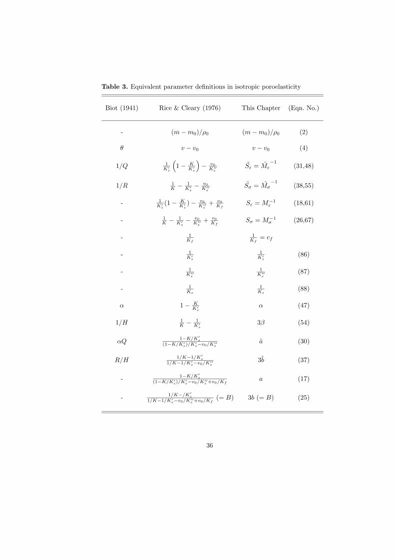
Table 3. Equivalent parameter definitions in isotropic poroelasticity
Biot (1941) Rice & Cleary (1976) This Chapter (Eqn. No.)
- (m−m0)/ρ0 (m−m0)/ρ0 (2)
θ v − v0 v − v0 (4)
1/Q 1K′
s
(1− K
K′s
)− v0
K′′s
Sε = Mε−1
(31,48)
1/R 1K −
1K′
s− v0
K′′s
Sσ = Mσ−1
(38,55)
- 1K′
s(1− K
K′s)− v0
K′′s
+ v0Kf
Sε = M−1ε (18,61)
- 1K −
1K′
s− v0
K′′s
+ v0Kf
Sσ = M−1σ (26,67)
- 1Kf
1Kf
= cf
- 1K′
s
1K′
s(86)
- 1K′′
s
1K′′
s(87)
- 1Ks
1Ks
(88)
α 1− KK′
sα (47)
1/H 1K −
1K′
s3β (54)
αQ1−K/K′
s
(1−K/K′s)/K′
s−v0/K′′s
a (30)
R/H1/K−1/K′
s
1/K−1/K′s−v0/K′′
s3b (37)
- 1−K/K′s
(1−K/K′s)/K′
s−v0/K′′s +v0/Kf
a (17)
- 1/K−/K′s
1/K−1/K′s−v0/K′′
s +v0/Kf(= B) 3b (= B) (25)
36
6 Gassmann’s Relation; Generalization andAlternative Forms
The most direct way to relate the drained and undrained moduli Cijkl andCuijkl is the following. We formally express the stress σij as a functionof εkl and m by writing the equation of state (12) or its linearized form(58) as σij = σij(εkl, µ(εkl,m)), assuming the function µ = µ(εkl,m) to begiven, e.g. in the form of the linear relation ρ0µ = −Mεαijεij +Mε∆m/ρ0,obtained by rewriting (59). Differentiating this function one gets
∂σij∂εkl
∣∣∣0m
= Cuijkl =∂σij∂εkl
∣∣∣0µ
+∂σij∂µ
∣∣∣0εkl
∂µ
∂εkl
∣∣∣0m
= Cijkl + αijakl,
where the derivatives have been evaluated as in (58) and (59); thus we arriveat (64).
Similarly, in establishing the relationship between drained and undrainedcompliances, one regards the strain as a function εij = εij(σkl, µ(σkl,m)).Making use of the definitions in (65) and (66), one obtains (70)
∂εij∂σkl
∣∣∣0m
= Suijkl =∂εij∂σkl
∣∣∣0µ
+∂εij∂µ
∣∣∣0εkl
∂µ
∂σkl
∣∣∣0m
= Sijkl − βijbkl.
In applications of poroelasticity theory one often desires to relate drainedto undrained properties, or undrained properties for an aqueous pore fluidto undrained properties for hydrocarbon pore fluids.18 This is the fluid sub-stitution problem that continues to be of great interest, in particular to ex-ploration seismologists studying 4-D seismic time-lapse methods (Carcioneand Tinivella, 2001). The classical problem considered in this context is es-sentially the derivation of a relationship between the drained and undrainedcompliances. This problem is solved by (70)1, but there are a number pointsto be made here. Consider first the form
Sijkl − Suijkl = Mσβijβkl =βijβkl
Sσ + v0cf(119)
of this result. This tells us that the two compliances can be calculatedin terms of each other, once the tensorial coefficient βij and the scalar
18The drained compliances are often referred to as dry compliances in this context, in
reference to the fact that the pore pressure remains constant in a drained deformation.
Note, however, that Biot’s notion of a wetted porous medium, as discussed in the above,
would be a more appropriate description of the state of a fluid-saturated material that
undergoes a drained deformation.
37
coefficient Mσ are known. Instead of measuring the latter directly, onecould also determine Sσ and cf independently. This also suggests a wayto account for a change of pore fluid. Although it would thus be desirableto perform a direct measurement of the coefficient Sσ by determining thechange in pore volume with pore fluid pressure of a sample at constant stress,the difficulty of such a measurement suggests an appeal to expression (91)as an alternative. Proceeding in this way, we also express the componentsβij by use of (93) in terms of the components S′ijkk; (119) then assumes theform
Sijkl − Suijkl =(Sijmm − S′ijmm)(Sklnn − S′klnn)1/K − 1/K ′s + v0(1/Kf − 1/K ′′s )
. (120)
This result was first given by Brown and Korringa (1975) and sometimesreferred to a ‘Brown-Korringa equation’ or ‘Brown-Korringa relation’. (Seealso Mavko et al. (1998) and Gueguen et al. (2004) for discussions of thisimportant relationship.) A particularly important point to bear in mindis that the components S′ijkk are understood to have been measured underΠ−loading conditions in accord with (95), unless of course one is dealingwith the special case of a micro-homogenous skeleton, such as a poroussingle crystal, with known compliances Ssijkl.
Much earlier, the first result of this kind was derived by Gassmann (1951)for isotropic materials. Gassmann’s relation is in fact identical with (106),but by use of (110) and (112) this may be brought into the form
1K− 1Ku
=(1/K − 1/K ′s)
2
1/K − 1/K ′s + v0(1/Kf − 1/K ′′s )(121)
which represents the isotropic version of (120).In the interesting more general case of an isotropic unjacketed response,
we have
Sijkl − Suijkl =[Sijmm − (1/3K ′s)δij ][Sklnn − (1/3K ′s)δkl]
1/K − 1/K ′s + v0(1/Kf − 1/K ′′s ). (122)
This may often be an acceptable approximation of relation (120), but it isone that must be verified experimentally in each case.
An alternative generalized Gassmann’s relation is given by (64), whichmay be written
Cuijkl − Cijkl =αijαkl
Sε + v0cf(123)
and here the possibility of a direct measurement of the Biot coefficient αijand of the specific storage capacities Sε or Sε = Sε + v0cf seems worth
38
considering. Where this proves impractical, there remains always the optionof bringing (123) into the form
Cuijkl − Cijkl =(δij − CijmnS′mnrr)(δkl − CklpqS′pqss)1/K ′s(1−K/K ′s) + v0(1/Kf − 1/K ′′s )
(124)
by substituting the expressions (94) and (117) for αij and Sε. In the caseof isotropy (123) reduces to (105) and this can now be expressed as
Ku −K =(1−K/K ′s)2
1/K ′s(1−K/K ′s) + v0(1/Kf − 1/K ′′s ), (125)
which is just another way of writing (121). Finally, in the special case ofan isotropic unjacketed response we may substitute (99) for αij in (124), toobtain
Cuijkl − Cijkl =(δij − Cijmm/3K ′s)(δkl − Cklnn/3K ′s)1/K ′s(1−K/K ′s) + v0(1/Kf − 1/K ′′s )
. (126)
Bibliography
Berge, P.A., and J.G. Berryman (1995). Realizability of negative pore com-pressibility in poroelastic composites. J. Appl. Mech. 62, 1053–1062.
Berryman, J.G. (1995). Mixture theories for rock properties. In: RockPhysics and Phase Relations. A Handbook of Physical Constants, editedby T.J. Ahrens, Am. Geophys. Union, Washington D.C., pp. 205–228.
Biot, M.A. (1941). General theory of three-dimensional consolidation.J. Appl. Phys. 12, 155–164.
Biot, M.A. (1955). Theory of elasticity and consolidation for a porousanisotropic solid. J. Appl. Phys. 26, 182–185.
Biot, M.A. (1956). Thermoelasticity and irreversible thermodynamics.J. Appl. Phys. 27, 240–253.
Biot, M.A. (1972). Theory of finite deformation of porous solids. IndianaUniv. Math. J. 21(7), 597–620.
Biot, M.A. (1973). Nonlinear and semilinear rheology of porous solids.J. Geophys. Res. 78, 4924–4937.
Biot, M.A., and D.G. Willis (1957). The elastic coefficients of the theory ofconsolidation. J. Appl. Mech. 24, 594–601.
Brown, R.J.S., and J. Korringa (1975). On the dependence of the elasticproperties of a porous rock on the compressibility of the pore fluid. Geo-physics 40, 608–616.
39
Callen, H.B. (1960). Thermodynamics, John Wiley, New York.Carcione, J.M., and U. Tinivella (2001). The seismic response to overpres-
sure: a modelling study based on laboratory, well and seismic data.Geophysical Prospecting 49, 523–539.
Carroll, M.M. (1979). An effective stress law for anisotropic elastic defor-mation. J. Geophys. Res. 84, 7510–7512.
Cheng, A.H.D. (1997). Material coefficients of anisotropic poroelasticity.Int. J. Rock Mech. Min. Sci. 34, 199–205.
Coussy, O. (2004). Poromechanics, John Wiley & Sons Ltd., Chichester UK.Detournay, E., and A.H.D. Cheng (1993). Fundamentals of poroelasticity.
In: Comprehensive Rock Engineering Vol. 2, edited by J. A. Hudson,Pergamon Press, Oxford, Chap. 5, pp. 113–171.
Gassmann, F. (1951). Uber die Elastizitat poroser Medien. Vierteljahrs-schr. Naturforsch. Ges. Zurich 96, 1–23.
Geertsma, J. (1957a). A remark on the analogy between thermoelasticityand the elasticity of saturated porous media. J. Mech. Phys. Solids 6,13–16.
Geertsma, J. (1957b). The effect of fluid pressure decline on volumetricchanges in porous rocks. Trans. AIME 210, 331–340.
Geertsma, J. (1966). Problems of rock mechanics in petroleum productionengineering. Proc. 1st Congr. Int. Society of Rock Mechanics, 585–594.
Green, D.H., and H.F. Wang (1986). Fluid pressure response to undrainedcompression in saturated sedimentary rocks. Geophysics 51, 948–956.
Green, D.H., and H.F. Wang (1990). Specific storage as a poroelastic coef-ficient. Water Resources Res. 26, 1631–37.
Gueguen, Y., L. Dormieux, and M. Bouteca (2004). Fundamentals ofPoromechanics. In: Mechanics of Fluid-Saturated Rocks, edited byY. Gueguen and M. Bouteca, Elsevier Academic Press, Burlington MA,pp. 1–54.
Jaeger, J.C., N.G.W. Cook, and R.W. Zimmerman (2007). Fundamentalsof Rock Mechanics (4th edition), Blackwell Publishing Ltd, Oxford, etc.
Kumpel, H-J. (1991). Poroelasticity: parameters reviewed. Geophys. J. Int.105, 783–799.
Mavko, G., T. Mukerji, and J. Dvorkin (1998). The Rock Physics Hand-book. Tools for Seismic Analysis in Porous Media. Cambridge U. Press,Cambridge UK.
McTigue, D.F. (1986). Thermoelastic response of fluid-saturated porousrock. J. Geophys. Res. 91, 9533–9542.
40
Nur, A., and J.D. Byerlee (1971). An exact effective stress law for elasticdeformation of rock with fluids. J. Geophys. Res. 76, 6414–6419.
Nye, J.F. (1957). Physical Properties of Crystals. Oxford University Press,Oxford etc., (reprinted in 1979).
Rice, J.R., and M.P. Cleary (1976). Some basic stress diffusion solutionsfor fluid-saturated elastic porous media with compressible constituents.Rev. Geophys. Space Phys. 14, 227–241.
Rudnicki, J.W. (1985). Effect of pore fluid diffusion on deformation andfailure of rock. In: Mechanics of Geomaterials, edited by E. Bazant,John Wiley & Sons Ltd., New York, Chap. 15, pp. 315–347.
Rudnicki, J.W. (2001). Coupled deformation-diffusion effects in the mechan-ics of faulting and failure of geomaterials. Appl. Mech. Rev. 54, 1–20.
Terzaghi, K., and O.K. Frohlich (1936). Theorie der Setzung von Ton-schichten, F. Deutike, Wien.
Thompson, M., and J.R. Willis (1991). A reformulation of the equations ofanisotropic poroelasticity. J. Appl. Mech. 58, 612–616.
Wang, H.F. (2000). Theory of Linear Poroelasticity with Applications toGeomechanics and Hydrogeology. Princeton University Press, Princetonand Oxford.
Weiner, J.H. (1983). Statistical Mechanics of Elasticity, John Wiley & Sons,New York.
Zimmerman, R.W., W.H. Somerton, and M.S. King (1986). Compressibilityof porous rocks. J. Geophys. Res. 91, 12,765–12,777.
41


