Embed Size (px)
Citation preview


Unit Operations ofParticulate Solids
Theory and Practice


Michelle Poliskie
Solar ModulePackagingPolymeric Requirementsand Selection
CRC Press is an imprint of theTaylor & Francis Group, an informa business
Boca Raton London New York
Unit Operations ofParticulate Solids
Enrique Ortega-Rivas
Theory and Practice
CRC Press is an imprint of theTaylor & Francis Group, an informa business
Boca Raton London New York

The Open Access version of this book, available at www.taylorfrancis.com, has been made available under a Creative Commons Attribution-Non Commercial-No Derivatives 4.0 license.
CRC PressTaylor & Francis Group6000 Broken Sound Parkway NW, Suite 300Boca Raton, FL 33487-2742
© 2012 by Taylor & Francis Group, LLCCRC Press is an imprint of Taylor & Francis Group, an Informa business
No claim to original U.S. Government works
Printed in the United States of America on acid-free paperVersion Date: 20110608
International Standard Book Number: 978-1-4398-4907-1 (Hardback)
This book contains information obtained from authentic and highly regarded sources. Reasonable efforts have been made to publish reliable data and information, but the author and publisher cannot assume responsibility for the validity of all materials or the consequences of their use. The authors and publishers have attempted to trace the copyright holders of all material reproduced in this publication and apologize to copyright holders if permission to publish in this form has not been obtained. If any copyright material has not been acknowledged please write and let us know so we may rectify in any future reprint.
Except as permitted under U.S. Copyright Law, no part of this book may be reprinted, reproduced, transmitted, or utilized in any form by any electronic, mechanical, or other means, now known or hereafter invented, including photocopying, microfilming, and recording, or in any information stor-age or retrieval system, without written permission from the publishers.
For permission to photocopy or use material electronically from this work, please access www.copy-right.com (http://www.copyright.com/) or contact the Copyright Clearance Center, Inc. (CCC), 222 Rosewood Drive, Danvers, MA 01923, 978-750-8400. CCC is a not-for-profit organization that pro-vides licenses and registration for a variety of users. For organizations that have been granted a pho-tocopy license by the CCC, a separate system of payment has been arranged.
Trademark Notice: Product or corporate names may be trademarks or registered trademarks, and are used only for identification and explanation without intent to infringe.
Visit the Taylor & Francis Web site athttp://www.taylorandfrancis.com
and the CRC Press Web site athttp://www.crcpress.com

v
Contents
Preface ................................................................................................................... xiiiAuthor .................................................................................................................. xvii
Part I Characterization of Particulate Systems and Relation to Storage and Conveying
1 Introduction .....................................................................................................31.1 Definitions of Unit Operations ............................................................31.2 Powder and Particle Technology ........................................................61.3 The Solid State: Main Distinctive Properties ....................................7
1.3.1 Primary Properties ..................................................................81.3.1.1 Particle Size and Shape ............................................91.3.1.2 Particle Density....................................................... 18
1.3.2 Packing Properties .................................................................231.3.2.1 Bulk Density ............................................................231.3.2.2 Other Packing Properties ...................................... 26
References ....................................................................................................... 29
2 Bulk Solids: Properties and Characterization ........................................ 312.1 Introductory Aspects .......................................................................... 312.2 Classification of Powders ................................................................... 32
2.2.1 Jenike’s Classification ............................................................332.2.2 Geldart’s Classification..........................................................34
2.3 Sampling............................................................................................... 372.4 Failure Properties ................................................................................48
2.4.1 Introduction ............................................................................482.4.2 Description of Failure Properties ........................................502.4.3 Experimental Determinations .............................................502.4.4 Other Important Properties .................................................. 61
2.5 Laboratory Exercise: Determination of Some Failure Properties of Powders ...........................................................652.5.1 Introduction ............................................................................652.5.2 Instrument and Materials .....................................................662.5.3 Shear Tester Operation ..........................................................662.5.4 Calculations and Report ....................................................... 67
2.6 Particle Size Analysis ......................................................................... 672.6.1 Introduction ............................................................................ 672.6.2 Definitions of Characteristic Linear Dimension ...............682.6.3 Types of Distributions ...........................................................68
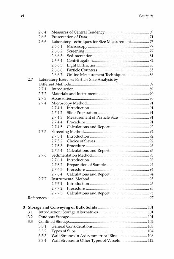
vi Contents
2.6.4 Measures of Central Tendency............................................. 692.6.5 Presentation of Data .............................................................. 712.6.6 Laboratory Techniques for Size Measurement .................. 76
2.6.6.1 Microscopy ..............................................................772.6.6.2 Screening .................................................................772.6.6.3 Sedimentation ......................................................... 812.6.6.4 Centrifugation......................................................... 822.6.6.5 Light Diffraction .....................................................852.6.6.6 Particle Counters ....................................................852.6.6.7 Online Measurement Techniques ........................86
2.7 Laboratory Exercise: Particle Size Analysis by Different Methods ............................................................................... 89
2.7.1 Introduction ............................................................................ 892.7.2 Materials and Instruments ...................................................902.7.3 Accessories ..............................................................................902.7.4 Microscopy Method ............................................................... 91
2.7.4.1 Introduction ............................................................ 912.7.4.2 Slide Preparation .................................................... 912.7.4.3 Measurement of Particle Size ............................... 912.7.4.4 Procedure ................................................................ 912.7.4.5 Calculations and Report ........................................ 92
2.7.5 Screening Method .................................................................. 922.7.5.1 Introduction ............................................................ 922.7.5.2 Choice of Sieves ...................................................... 922.7.5.3 Procedure ................................................................ 932.7.5.4 Calculations and Report ........................................ 93
2.7.6 Sedimentation Method.......................................................... 932.7.6.1 Introduction ............................................................ 932.7.6.2 Preparation of Sample ........................................... 942.7.6.3 Procedure ................................................................ 942.7.6.4 Calculations and Report ........................................ 94
2.7.7 Instrumental Method ............................................................ 952.7.7.1 Introduction ............................................................ 952.7.7.2 Procedure ................................................................ 952.7.7.3 Calculations and Report ........................................ 95
References ....................................................................................................... 97
3 Storage and Conveying of Bulk Solids .................................................. 1013.1 Introduction: Storage Alternatives ................................................. 1013.2 Outdoors Storage ............................................................................... 1013.3 Confined Storage ............................................................................... 102
3.3.1 General Considerations ....................................................... 1033.3.2 Types of Silos ........................................................................ 1043.3.3 Wall Stresses in Axisymmetrical Bins .............................. 1083.3.4 Wall Stresses in Other Types of Vessels ........................... 112

Contents vii
3.3.5 Natural Discharge from Silos ............................................ 1123.3.5.1 Flow Theories ........................................................ 1133.3.5.2 Hopper Opening for Coarse Bulk Solids .......... 1163.3.5.3 Hopper Opening for Fine Bulk Solids .............. 120
3.3.6 Assisted Discharge .............................................................. 1233.3.6.1 Types of Discharge ............................................... 1233.3.6.2 Passive Devices ..................................................... 1233.3.6.3 Active Devices ...................................................... 123
3.3.7 Feeders for Discharge Control ........................................... 1273.3.7.1 Feeders Description ............................................. 1273.3.7.2 Charge and Power Calculations ......................... 1283.3.7.3 Discharge Control in Feeders ............................. 130
3.3.8 Other Design Factors ........................................................... 1303.4 Laboratory Exercise: Evaluation of Wall Loads in Silos .............. 134
3.4.1 Introduction .......................................................................... 1343.4.2 Equipment and Materials ................................................... 1343.4.3 Instruments and Apparatuses ........................................... 1343.4.4 Procedure .............................................................................. 1343.4.5 Calculations and Report ..................................................... 135
3.5 Bulk Solids Conveying ..................................................................... 1353.5.1 Introduction .......................................................................... 1353.5.2 Belt Conveyors ...................................................................... 1363.5.3 Chain Conveyors .................................................................. 143
3.5.3.1 Scraper and Apron Conveyors ........................... 1453.5.3.2 Bucket Elevators ................................................... 148
3.5.4 Screw Conveyors .................................................................. 1513.5.5 Pneumatic Conveying ......................................................... 155
3.5.5.1 Introduction: Types of Conveyors ...................... 1553.5.5.2 Dense-Phase Systems .......................................... 1573.5.5.3 Dilute-Phase Systems ........................................... 1593.5.5.4 Design and Selection of Dilute-Phase Systems ........................................... 163
3.6 Laboratory Exercise: Pneumatic Conveying Characteristics of Different Granules ............................................ 1713.6.1 Introduction .......................................................................... 1713.6.2 Equipment and Materials ................................................... 1713.6.3 Procedure .............................................................................. 1713.6.4 Calculations and Report ..................................................... 172
References ..................................................................................................... 173
II Part Bulk Solids Processing
4 Size Reduction ............................................................................................. 1794.1 Fundamental Principles of Comminution ..................................... 179

viii Contents
4.1.1 Introductory Aspects........................................................... 1794.1.2 Forces Involved in Size Reduction..................................... 1804.1.3 Properties of Comminuted Materials ............................... 181
4.2 Energy Requirements in Comminution ........................................ 1824.2.1 Rittniger’s Law ..................................................................... 1834.2.2 Kick’s Law ............................................................................. 1834.2.3 Bond’s Law and Work Index .............................................. 184
4.3 Size Reduction Equipment ............................................................... 1844.3.1 Classification ......................................................................... 1844.3.2 Characteristics ...................................................................... 184
4.3.2.1 Crushers ................................................................. 1854.3.2.2 Rollers Mills .......................................................... 1884.3.2.3 Hammer Mills ...................................................... 1894.3.2.4 Disc Attrition Mills .............................................. 1894.3.2.5 Tumbling Mills ..................................................... 1914.3.2.6 Other Types of Mills ............................................ 192
4.3.3 Operation of Equipment ..................................................... 1954.4 Criteria for Selecting Size Reduction Processes ...........................200
4.4.1 Characteristics of Raw Materials ....................................... 2014.4.2 Feeding and Discharge Control ......................................... 2014.4.3 Moisture ................................................................................ 2024.4.4 Heat Generation and Removal ........................................... 2024.4.5 Summary of Criteria and Main Applications .................. 203
4.5 Laboratory Exercise: Determination of Reduction Relations Using a Hammer Mill .................................. 204
4.5.1 Introduction .......................................................................... 2044.5.2 Equipment and Materials ................................................... 2044.5.3 Instruments........................................................................... 2054.5.4 Screen Analysis .................................................................... 2054.5.5 Operation of the Hammer Mill .......................................... 2054.5.6 Calculations and Report ..................................................... 205
References ..................................................................................................... 206
5 Size Enlargement ........................................................................................ 2075.1 Introduction: Agglomeration Processes ........................................ 2075.2 Aggregation Fundamentals: Strength of Agglomerates ............. 2075.3 Agglomeration Methods .................................................................. 212
5.3.1 Tumbling Agglomeration ................................................... 2125.3.2 Pressure Agglomeration: Compaction .............................. 2145.3.3 Equipment Operation Variables ........................................ 216
5.4 Selection Criteria for Agglomeration Methods............................. 2195.4.1 Raw Materials Characteristics ........................................... 2195.4.2 Product Properties ............................................................... 2215.4.3 Technique Options............................................................... 221
5.5 Design Aspects of Agglomeration Processes ................................222

Contents ix
5.6 Applications ....................................................................................... 2245.7 Laboratory Exercise: Comparing Methods for
Tumbling Agglomeration of Powders ............................................ 2245.7.1 Introduction .......................................................................... 2245.7.2 Equipment and Materials ...................................................2255.7.3 Instruments...........................................................................2255.7.4 Measurement of Particle Size Distributions ....................2255.7.5 Operation of the Drum Agglomerator ..............................2255.7.6 Operation of the Pan (Disc) Agglomerator .......................2255.7.7 Friability Test ........................................................................ 2265.7.8 Calculations and Report ..................................................... 226
References ..................................................................................................... 226
6 Mixing ...........................................................................................................2296.1 Introduction .......................................................................................2296.2 Blending Mechanisms ......................................................................2306.3 Statistical Approach of Mixing Processes ..................................... 231
6.3.1 Sampling ............................................................................... 2326.3.2 Blending Quality: Mixing Indexes and Mixing Rate ......................................233
6.4 Mixing Equipment ............................................................................ 2396.4.1 Tumbling Mixers .................................................................. 2396.4.2 Horizontal Trough Mixers .................................................. 2406.4.3 Vertical Screw Mixers .......................................................... 241
6.5 Design and Selection Factors ........................................................... 2416.6 Laboratory Exercise: Determination of Blending
Indices for Different Tumbling Mixers .......................................... 2446.6.1 Introduction .......................................................................... 2446.6.2 Equipment and Materials ................................................... 2446.6.3 Instruments or Apparatuses .............................................. 2446.6.4 Operation of the Mixers ...................................................... 2456.6.5 Calculations and Report ..................................................... 245
References ..................................................................................................... 246
7 Fluidization .................................................................................................. 2497.1 Theoretical Fundamentals ............................................................... 249
7.1.1 Bulk Density and Porosity of Beds ....................................2507.1.2 Fluid Flow through Solids Beds ........................................2507.1.3 Mechanism of Fluidization: Aggregative and Particulate ............................................... 251
7.2 Fluidized Regimes ............................................................................2537.2.1 Pressure Drop–Velocity Relationship ...............................2547.2.2 Incipient Fluidization and Minimum Fluidizing Velocity ...........................................2567.2.3 Heterogeneous Fluidization: Bubbling ............................. 261

x Contents
7.2.4 Spouted Beds ........................................................................2647.3 Applications of Fluidization ............................................................ 267
7.3.1 Applications in the Petroleum and Chemical Industries ............................................................ 2687.3.2 Fluidized-Bed Combustion ................................................ 2687.3.3 Drying in Fluidized Beds ................................................... 2697.3.4 Coating of Particles and Particulates ................................ 272
7.4 Laboratory Exercise: Fluidized-Bed Coating of Food Particulates ............................................................................... 276
7.4.1 Introduction .......................................................................... 2767.4.2 Equipment and Materials ................................................... 2767.4.3 Instruments and Apparatuses ........................................... 2767.4.4 Operation of the Fluidized Bed ......................................... 2767.4.5 Evaluation of the Coating Thickness ................................2777.4.6 Friability Test ........................................................................2777.4.7 Calculations and Report .....................................................277
References ..................................................................................................... 278
Part III Separation Techniques for Particulate Solids
8 Introductory Aspects .................................................................................2838.1 Different Mixtures Relevant in Industry .......................................2838.2 Classification of Separation Techniques ........................................2838.3 Specific Techniques for Granular Materials ..................................284References ..................................................................................................... 286
9 Solid Mixtures ............................................................................................. 2879.1 Screening ............................................................................................ 287
9.1.1 Basic Principles ..................................................................... 2879.1.2 Design and Selection Criteria ............................................ 2899.1.3 Equipment Used ................................................................... 296
9.2 Electromagnetic Separation ............................................................. 3019.2.1 Basic Principles ..................................................................... 3019.2.2 Equipment and Applications .............................................3039.2.3 Selection Criteria ..................................................................306
9.3 Electrostatic Separation .................................................................... 3079.3.1 Basic Principles ..................................................................... 3079.3.2 Equipment and Applications .............................................3099.3.3 Applications in Fine Particulate Systems ......................... 312
9.4 Laboratory Exercise: Efficiency of Separation on Single-Stage Screening ..................................................................... 312
9.4.1 Introduction .......................................................................... 3129.4.2 Equipment and Materials ................................................... 313

Contents xi
9.4.3 Instruments or Apparatuses .............................................. 3139.4.4 Screening Procedure ........................................................... 3139.4.5 Calculations and Report ..................................................... 314
References ..................................................................................................... 316
10 Solid–Fluid Systems .................................................................................. 31710.1 Introduction: Simultaneous Flow of Fluids and Solids ............... 317
10.1.1 Classification of Fluids ........................................................ 31710.1.2 Dynamics of Particles Submerged in Fluids .................... 320
10.2 Separation Efficiency ........................................................................ 32410.2.1 Evaluation of Efficiency ...................................................... 32410.2.2 Total Gravimetric Efficiency ............................................... 32510.2.3 Partial Gravimetric Efficiency ............................................ 32710.2.4 Grade Efficiency and Cut Size ............................................ 329
10.3 Solid–Gas Separations ......................................................................33310.3.1 Introduction ..........................................................................33310.3.2 Use of Cyclones ....................................................................334
10.3.2.1 Description of the Process...................................33410.3.2.2 Theoretical Aspects ..............................................33610.3.2.3 Operating Variables ............................................. 33710.3.2.4 Applications ..........................................................340
10.3.3 Air Classifiers .......................................................................34010.3.3.1 Description of the Technique .............................34010.3.3.2 Theoretical Aspects .............................................. 341
10.3.3 Operation and Applications ...............................................34310.3.4 Gas Filters ..............................................................................345
10.3.4.1 Description of the Process...................................34510.3.4.2 Operation Characteristics and Applications ...... 348
10.3.5 Scrubbers ...............................................................................34810.3.5.1 Process Description ..............................................34910.3.5.2 Equipment and Applications ..............................349
10.3.6 Other Techniques ................................................................. 35110.3.6.1 Settling Chambers ................................................ 35110.3.6.2 Electrostatic Separators ....................................... 352
10.4 Solid–Liquid Separation Techniques ..............................................35310.4.1 Properties of Suspensions: Rheology and Flow ..............353
10.4.1.1 Laboratory Exercise: Rheograms of Suspensions ................................. 359
10.4.2 Pretreatment of Suspensions: Coagulation and Flocculation ...........................................................................360
10.4.3 Selection of Specific Techniques ........................................ 36210.4.3.1 Laboratory Exercise: Settling Tests to Select a Proper Technique ......36510.4.3.2 Calculations and Report ......................................366
xii Contents
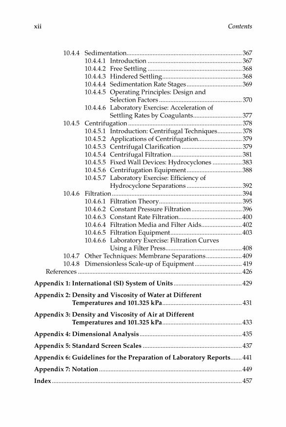
10.4.4 Sedimentation....................................................................... 36710.4.4.1 Introduction .......................................................... 36710.4.4.2 Free Settling ..........................................................36810.4.4.3 Hindered Settling .................................................36810.4.4.4 Sedimentation Rate Stages .................................. 36910.4.4.5 Operating Principles: Design and
Selection Factors ................................................... 37010.4.4.6 Laboratory Exercise: Acceleration of
Settling Rates by Coagulants .............................. 37710.4.5 Centrifugation ...................................................................... 378
10.4.5.1 Introduction: Centrifugal Techniques ............... 37810.4.5.2 Applications of Centrifugation........................... 37910.4.5.3 Centrifugal Clarification ..................................... 37910.4.5.4 Centrifugal Filtration ........................................... 38110.4.5.5 Fixed Wall Devices: Hydrocyclones ..................38310.4.5.6 Centrifugation Equipment ..................................38810.4.5.7 Laboratory Exercise: Efficiency of
Hydrocyclone Separations .................................. 39210.4.6 Filtration ................................................................................ 394
10.4.6.1 Filtration Theory ................................................... 39510.4.6.2 Constant Pressure Filtration ............................... 39610.4.6.3 Constant Rate Filtration.......................................40010.4.6.4 Filtration Media and Filter Aids.........................40210.4.6.5 Filtration Equipment ............................................40310.4.6.6 Laboratory Exercise: Filtration Curves
Using a Filter Press ...............................................40810.4.7 Other Techniques: Membrane Separations ......................40910.4.8 Dimensionless Scale-up of Equipment ............................. 419
References .....................................................................................................426
Appendix 1: International (SI) System of Units ..........................................429
Appendix 2: Density and Viscosity of Water at Different Temperatures and 101.325 kPa ................................................. 431
Appendix 3: Density and Viscosity of Air at Different Temperatures and 101.325 kPa .................................................433
Appendix 4: Dimensional Analysis ...............................................................435
Appendix 5: Standard Screen Scales ............................................................. 437
Appendix 6: Guidelines for the Preparation of Laboratory Reports ....... 441
Appendix 7: Notation ........................................................................................449
Index ..................................................................................................................... 457

xiii
Preface
The idea of writing this book was conceived many years ago when the author started teaching unit operations in the undergraduate program of chemical engineering at the Autonomous University of Chihuahua, even prior to attending the then Postgraduate School of Studies in Powder Technology at the University of Bradford. The importance, relevance and prevalence of the topic of particle technology remain up-to-date. Studies by the Rand Corporation in the 1980s identified substantial differences in the scale-up and start-up performance of plants processing powders versus those pro-cessing liquids or gases. Particularly, in 1985, the Rand Report surveyed 40 US plants and found out that start-up times were 200–300% of those pre-dicted (compared to 20% for fluid-based plants) and only achieved approxi-mately 50% of their designed throughput. By comparison, most fluid-based processes reached 90% of planned output over the same period. Some of the reasons described at the time of the report were related to an inadequate understanding of the behavior of particle systems, which is sensitive to pro-cess scale or process history in ways that would not be expected by engi-neers familiar with only liquid or gas systems.
The response to overcome these difficulties came by way of promoting research, programs of study, and other activities in the field of powder or particle technology worldwide. Substantial advancements have been achieved through all these initiatives but, apparently, many of the reported reasons for this unequal understanding of powder-based processes, as com-pared to fluid-based processes, remain up to today. This perception is implied by a current need of consultancy in the subject by different types of indus-tries worldwide. In a recent seminar at the Autonomous University of Chihuahua, Richard Farnish, consulting engineer at the Wolfson Centre for Bulk Solids Handling Technology of the University of Greenwich, strongly supported this perception by sharing with the audience the many examples of his consulting activities in the subject for at least a decade.
An obvious outcome of the upsurge of academic activities related to par-ticle technology that started in the 1980s but keep momentum to date is the production of scientific literature about this particular topic. Papers, book chapters, encyclopedia contributions, reports, reference books, and textbooks have been produced during these years. The contribution represented by this work intends to add to the literature on the subject by trying to provide a textbook aimed at training practicing engineers in bulk solids handling and processing who might be, apparently, on high demand for years to come. The idea of writing the book started realization of the need for complemen-tary literature on the subject, as already mentioned. The great opportunity that the author had was time to learn from an enviable academic staff

xiv Preface
of premium quality and who had an undisputable pioneering role in estab-lishing the discipline known as particle technology. This sparked in the author a vested interest and a great fascination for the subject. In presenting this work I took knowledge and inspiration directly from my PhD thesis supervisor, Lado Svarovsky, but had close contact with some of the other “big names” of the time: John Williams, Derek Geldart, Nayland Stanley-Wood, Arthur Hawkins, and a young Martin Rhodes, initiating his career focused on fluidization. Drawing an analogy, the senior academic staff of the University of Bradford at the time would resemble the pitching staff of the US baseball team, the Atlanta Braves of the 1990s, or the current tennis Spanish team competing for the Davis Cup.
The book deals with unit operations in chemical engineering involving handling and processing of particulate solids. In the literature, as well as in many higher-education study programs, unit operations have been classi-fied as heat transfer and mass transfer unit operations with excellent text-books written following such criteria. There are a number of unit operations, which have been left out of these mentioned classifications, related to mechanical operations and fluid flow phenomena, but mostly coinciding with the subjects studied by the engineering discipline of particle technol-ogy. Commonly, most traditional unit operations books cover in great detail those unit operations involving heat and mass transfer, leaving the opera-tions dealing with particulate solids at a mere introductory level. Most of these books are normally written as textbooks. On the other hand, books classified in the disciplines of powder technology, particle techno logy, or bulk solids handling, cover in great detail all unit operations involving particulate solids and granular materials, but are generally written as refer-ence books and not as textbooks.
This work is aimed at filling a gap in the topic of unit operations involv-ing particulate solids as it is written as a textbook but may be considered a reference book also. It is presented in the chemical engineering unit opera-tions fashion of many textbooks, but with the additional feature of includ-ing suggested laboratory experiments. It has been written for students, undergraduates and postgraduates, as well as for educators and practicing chemical engineers. Readers will find it useful because it represents a suit-able textbook for a series of courses related to particle technology taught worldwide in universities and higher-education institutions.
The work is divided into three main themes: characterization of particu-late systems and relation to storage and conveying, bulk solids processing, and separation techniques for particulate solids. In the first part of the book, primary and secondary properties of particles and particulate systems are reviewed and analyzed thoroughly, focusing on their characterization and the effects on selection and design of silos and conveyors. The main purpose is to provide the student with theoretical and practical tools to understand the behavior of powders and pulverized systems. The second part deals with the main industrial operations of dry solids processing in order to give

Preface xv
insight into the operation principles of the most important technologies to handle dry solids in bulk. The theoretical principles are coupled with labora-tory exercises to provide information and skills to operate, optimize, and innovate particle processing technologies. The third segment of the book refers to applications of a very interesting subject, which sometimes has not been properly covered in higher education engineering programs: two-phase and multiphase flow. Many engineering processes deal with these types of systems but, since the topic may be considered part of fluid mechanics, rheol-ogy, or particle technology, it is often left out of educational programs. All the relevant systems in industrial processes combining two different compo-nents of the state of matter are described, and the technologies involved in separating phases by purely mechanical means, are studied in the final part of the book. The emphasis is, again, on providing balanced theoretical and practical components to learn and understand the operation of machinery and equipment to carry out relevant industrial operations such as centrifu-gation, filtration, and membrane separations.
This work was originally written in Spanish, but publishers in this lan-guage from Spain to Argentina and Mexico, did not find the project suitable or attractive. Some time passed, however, in the process of promoting the book with publishers in the Spanish language. The decision was thus made to translate the work into English and the response from publishers in English was prompt and positive. The whole project, from its origins in Spanish to its transformation into English has, therefore, taken time and involved extra work. Indeed, no man is an island, and many people at differ-ent times have contributed, voluntarily or involuntarily, to this project.
The author takes great pleasure in acknowledging the different partici-pants in the project of writing this book. The main reason and inspiration for planning, developing, and concluding the work are, of course, the students of the last decades sitting at the course of Unit Operations I in the Chemical Engineering Program of the Autonomous University of Chihuahua. The first draft, from handwritten notes prepared to teach this undergraduate course, was created using first versions of the current word processors by Carmelita Gonzalez, then secretary of the postgraduate program in Food Technology of the Autonomous University of Chihuahua. Many students from both the undergraduate program in chemical engineering and the postgraduate pro-gram in food technology have prepared excellent laboratory reports at dif-ferent times and some of them were used in preparing several of the laboratory exercises for the book. It would be impossible to mention all of them by name but their contribution is valued. Jocelyn Sagarnaga-Lopez and Hugo Omar Suarez-Martinez, MSc supervisees of the author and recent recipients of a State Award on Scientific Merit for their degree theses, wrote a chapter along with him on solid–liquid separations for a book on food pro-cessing and some aspects of the theoretical part of it were used in preparing the last chapter of this book. A useful hand in the task of translating the book and making sense of such translation was given by Israel Marquez, a student

xvi Preface
in the chemical engineering program at the sister institution of the Chihuahua Institute of Technology.
Last, but not least, sincere and fondest appreciation is given to my wife Sylvia, my daughters Samantha and Christina, who suffer the inevitable reduction of time shared with them due to the extra investment of time for the book writing project.
Enrique Ortega-RivasChihuahua, Mexico

xvii
Author
Professor Enrique Ortega-Rivas holds an MSc in food process engineering from the University of Reading and a PhD in chemical engineering from the University of Bradford. He is currently a professor at the Autonomous University of Chihuahua, México, and has held a visiting scientist appoint-ment at Food Science Australia and a visiting lectureship at Monash University, Australia. He was also a Fulbright scholar, acting as adjunct associate professor, at Washington State University. He has been awarded the status of national researcher, the maximum recognition that the Mexican government confers on academics based on their research achievements. He was shortlisted for the 2009 IChemE Innovation and Excellence Award in Food and Drink Processing and he is recipient of the 2010 Chihuahua Award in Technological Sciences. He has taught food process engineering in Chihuahua, Washington State and Monash, while other teaching topics have included unit operations involving particulate materials, as well as heat and mass transfer operations. His research interests include food engi-neering, particle technology, and solid–fluid separation techniques. He has focused his research efforts on the biological applications of hydrocyclones, in food powder processing, and in the employment of pulsed electric fields to pasteurize fluid foods.
Dr. Ortega-Rivas has served on many committees for international scien-tific events and performed peer reviews for national and international research funding organizations. He has also published numerous papers in international indexed journals, in addition to chapters in books and contri-butions to encyclopedias. He is the coauthor of the book Food Powders: Physical Properties, Processing, and Functionality published by Springer and editor of the book Processing Effects on Safety and Quality of Foods published by CRC Taylor & Francis. He is a member of the editorial boards of Food and Bioprocess Technology: An International Journal, Food Engineering Reviews, and The Open Food Science Journal. He reviews manuscripts for different inter national journals.

Part I
Characterization of Particulate Systems
and Relation to Storage and Conveying


3
1Introduction
1.1 Definitions of Unit Operations
The term unit operation has been used to describe a physical and/or mechan-ical procedure occurring parallel to a chemical reaction known as unit pro-cess, which happens in diverse materials processing industries. In order to understand this term properly, one should bear in mind that modernly struc-tured industries were shaped during the great industrial revolution that started in England in the eighteenth century. With the invention of the steam engine, some industries developed and grew in complexity as other energy sources, such as oil and electricity, were incorporated (Valiente and Stivalet, 1980). In modern economics, there are four main components in economic activities of a nation or region:
Primary sector:• extraction of natural resources (agriculture, fishing, mining, etc.)Secondary sector:• transformation of primary products (industry)Tertiary sector:• services (commerce, banking, transportation, etc.)Quaternary sector:• technological exploitation (research, design, and development)
The industrial sector needs to be further classified, but that would be a difficult task. A broad general categorization could be considered, however, as follows:
Manufacturing industry (assembled goods, automotive industry, •etc.)Construction industry (building construction, industrial construc-•tion, etc.)Materials processing industry•
The materials processing industry receives diverse raw materials to be trans-formed directly from the primary sector, either for direct consumption as

4 Unit Operations of Particulate Solids
finished products or for further transformation in some other types of indus-tries. The materials processing industry may be divided into four categories:
Chemical industry•Pharmaceutical industry•Food industry•Metallurgy industry•
In many industrial plants that process materials, a fundamental aspect of their operation is a chemical reaction known as unit process, such as oxygen-ation, hydrogenation, or polymerization. In order for a particular reaction to be carried out, a series of controlled steps to create optimal conditions are required. These steps or maneuvers are the physical and/or mechanical pro-cesses mentioned before (evaporation, distillation, pulverization, etc.) and are known as unit operations. The term unit operation arose from the need to standardize and systematize the teaching of chemical engineering as a discipline, due to the growth of the industry activity generated by the indus-trial revolution. A sort of tailor-made appropriate professional was required to operate chemical processing plants and promote a harmonic development of the materials processing industry. In 1887 George E. Davis proposed, in a famous series of 12 lectures at Manchester Technical School in England, the creation of a special career to cater for the growing chemical processing industry. Davis worked as an inspector for the Alkali Act of 1863, a very early piece of environmental legislation that required soda manufacturers to reduce emissions to the atmosphere. Davis also identified broad features common to all chemical factories, and he published his influential Handbook of Chemical Engineering (Davis, 1904) that roughly defined chemical engineer-ing as a profession. His lectures were criticized for being common place know-how observed around operating practices used by British chemical industries at the time. Davis’ ideas were, however, fundamental in initiating new thinking in the US chemical industry and sparking, eventually, the launching of chemical engineering study programs at several US universi-ties. Chemical engineering courses, organized by Lewis M. Norton, were taught by 1888 at the Massachusetts Institute of Technology (MIT). In 1891, the Department of Chemistry at MIT granted seven Bachelor’s degrees for Chemical Engineering, the first of their kind to be bestowed in the world. Almost at the same time, chemical engineering courses were offered at Pennsylvania State University in 1892, at Tulane University in 1894, and at Michigan University in 1898 (Valiente and Stivalet, 1980).
The pioneering courses of the chemical engineering degree programs con-sisted of deep knowledge of chemistry and physics complemented by courses of mechanical engineering and descriptive courses about equipment and important industry processes. As soon as the graduates began practicing, they realized about flaws and inconsistencies in their formation. The courses

Introduction 5
they received were descriptive but in practice they needed to make engineer-ing. They needed to know how to design equipment, how to calculate the size of a new plant, and so on. This served to discuss the teaching of chemi-cal engineering again in the schools. From these discussions, the concept of unit operation was originated, attributed to Arthur D. Little (Brown, 2005) who acted as president of the Inspecting Committee of the Department of Chemistry and Chemical Engineering at MIT. Such concepts may be defined textually as: “Any chemical process, at any scale, may be reduced to a coordi-nated series of what may be called unit operations, such as pulverize, dry, roast, crystallize, filter, evaporate, electrolyze, and so on. The number of these operations is not big and only a few of them is involved in a particular process” (Valiente and Stivalet, 1980, p. 35). Unit operations nowadays are diverse, since new types of industries have arisen, some consisting of very specific features. A classification of unit operations is not an easy task and some can be found in literature. The criteria used to categorize unit opera-tions are varied and may include types of phases involved in a process, mass transfer or heat transfer possibility, governing force (e.g., physical or mechan-ical) in an operation, and so on.
In general terms, the book by Walker et al. (1937) could be recognized as the first formal text of chemical engineering and the original work of McCabe and Smith (1956) as the most widely recognized and used text for educational purposes. Also, Perry’s Chemical Engineers’ Handbook (Green and Perry, 2008) is considered as the classical reference chemical engineering. An inspection to all of these classical works would reveal that the most widely studied unit operations are those involving heat transfer such as evaporation, mass trans-fer, for example, extraction, and combined heat and mass transfer, for exam-ple, drying. This trend is reasonable since, as mentioned before, the first chemical engineers had to optimize processes of the main industries of the time (acids, alkalis, explosives, textiles, cellulose, paper, etc.) in which heat and mass transfer operations predominate. They had to evaluate the thermo-dynamic and kinetic constants required to be able to work with the immense number of fluids involved in those chemical processing industries.
As the first industrial processes grew more complex, the industry activity was multiplied and sophisticated and new and varied industries appeared. In such a changing reality, chemical engineers realized that, in practice, cer-tain processes previous or subsequent to the unit process that were previ-ously overlooked also had great importance in the overall efficiency of the operation. These previous and subsequent steps represent a series of physi-cal operations that participate, mainly, in the storage and distribution of materials through a whole processing line. It was also observed that a series of operations not involving fluids, but granular solids instead, had been neglected for lacking the same response to heat or phase change, common in fluids in traditional operations (evaporation, condensation, drying, etc.). Furthermore, it was recognized that numerous granular solids and particulate materials intervene in a series of industrial processes, both as raw material
6 Unit Operations of Particulate Solids
or as finished products. There was awareness that many of these processes, or part of them, involved bulk solids handling and processing of solids. The understanding of behavior of particulate materials and industrial powders, within chemical engineering, did not have the same degree of advancement showed by fluids. In such a way, a need emerged for adapting teaching prac-tice and research activities in chemical engineering, as a way to contribute to the advancement of knowledge in powder handling and processing.
1.2 Powder and Particle Technology
The negligence in the study of the bulk solid state of matter was serious by the 1960s, and hence there was a critical need of growth based on research direc-tions detected by an integrated interdisciplinary approach to problems in this subject. It has been argued that powder technology came out as an academic discipline in Germany during the 1960s (Tardos, 1995). Other European coun-tries, such as the United Kingdom and the Netherlands followed suit and, like Germany, promoted work in academic groups of the recently created disci-pline. By the same time, Japan and Australia joined the trend, while in the United States, it was not until the 1980s that awareness about the lack of pro-fessional training in the area arose (Ennis et al., 1994). Directives of DuPont emphasized that 60% of the 3000 products their industries handled were in the form of particles and, therefore, their process engineers required addi-tional and exhaustive training. Partly for this reason, the National Science Foundation assigned resources for the establishment of the discipline in the study plans of chemical engineering of some universities. Research efforts in powder technology initiated from the time the discipline was established. European and Asian professional association and societies recognized its importance since then. Some of these associations, such as the Institution of Chemical Engineers (IChemE) and the Society of Chemical Industry in the United Kingdom have included established research groups in the topic, and have organized meetings and conferences on a regular basis. In the United States it was only until 1992 when a division, known as the Particle Technology Forum, was formed within the American Institute of Chemical Engineers. In a more global context, diverse international associations organize conferences and congresses on powder technology with delegates from around the world attending to present the most advanced developments in the area. While in Europe, Japan, and Australia the discipline was known initially as powder technology, in the United States it was given the name of particle technology. Nowadays, this latter term is most commonly used.
Regardless of how it is denominated, powder or particle technology is a branch of engineering dealing with the systematic study of particulate materials in a broad sense, whether in dry form or suspended within some
Introduction 7
fluid. For this reason, the interests of this discipline are numerous and com-prise operations of characterization, storage, conveying, mixing, fluidization, classification, agglomeration, and so on, of powders and particulate systems. Since many biphasic and multiphasic fluids are handled in many materials processing industries, a series of separation techniques, such as filtration and centrifugation, are also relevant in the study of particle technology. Finely divided and pulverized solids possess certain characteristics that make them different from chunky solids and, so, they cannot be fully understood under the discipline of materials science. Also, although under certain conditions they may flow, they cannot be addressed either by classic rheology for their study and research. In such a way, this branch of engineering has been devel-oped alongside other related branches and the discoveries brought by the study of particulate systems focusing on the particle technology principles has resulted in benefits for different industrial processes, including manu-facturing of chemicals, pharmaceuticals, foodstuffs, ceramics, and so on.
The first book published in the powder technology field was possibly the one authored by Dallavelle (1943) in the early 1940s, which contained basically all of the topics related to particle technology previously mentioned. Orr (1966) published another text which widened the coverage of the topics in Dallavelle’s book. Beddow (1981) wrote a third known text in particle technology, which has been extensively used for teaching purposes for many years. Some other books have been published in the general area of powder technology (Rhodes, 1990), as well as in related topics of particle size measurement (Allen, 1997), fluidization (Geldart, 1986), and separation techniques (Svarovsky, 2000). An excellent treatise on powders and bulk solids is the book by Schulze (2007), which includes properties, handling and flow in a single volume. As far as it could be surveyed, the focus of treating the topics of powder technology as unit operations has only been presented by Orr (1966).
1.3 The Solid State: Main Distinctive Properties
The properties of the solid state may be approached from different points of view. Properties of solids in large pieces differ from properties of particulate solids. The most important properties of pieces of solids include density, hardness, fragility, and tenacity (Brown, 2005). The density is defined as the mass by volume unit, while the hardness measures the resistance of the sol-ids to be scratched. A solid hardness scale was proposed by Mohs (Brown, 2005) and can be listed as follows:
1. Talc 2. Gypsum 3. Calcite

8 Unit Operations of Particulate Solids
4. Fluorite 5. Apatite 6. Orthoclase feldspar 7. Quartz 8. Topaz 9. Corundum 10. Diamond
In the above scale, each mineral scratches the previous. It is used to make reference to this chart to evaluate the hardness of some other known materi-als. For example, the hardness of ordinary glass is 5.8. The fragility is a prop-erty representing how easy a substance may be crumbled or broken by impact. It does not necessarily have a direct relation with hardness. Gypsum, for instance, is soft but not fragile. Finally, the tenacity is known as the prop-erty the metals and alloys present to resist collisions.
The molecular structure of solids determines some other features, such as shape of particles. Pieces of solids fracture following exfoliation planes deter-mined by its inner molecular arrangement. For example, galena breaks into cubes, graphite into platelet shape, and magnetite into approximate rounded grains. It also depends on structure the resistance that certain material offers to slide onto another material, known as friction. The coefficient of friction is defined as the relation between the parallel force to the rubbing surface in the direction of the movement, and the perpendicular force to the rubbing surface and normal to the movement direction.
A material is considered a powder if it is composed of dry, discrete parti-cles with a maximum dimension of less than 1000 μm (British Standards Institution, 1993), while a particle is defined by the McGraw-Hill Dictionary of Scientific and Technical Terms (2003, p. 1537) as “any relatively small sub-division of matter, ranging in diameter from a few angstroms to a few milli-meters.” These two definitions present a diffuse perspective upon which collection of individual entities may be identified as a powder or, simply, as a system of particles. In any case both groups of individual entities represent bulk materials of relevance in many industrial processes and efficient and reliable methods for characterizing them are needed in research, academia and industry. For convenience, properties of powder and particulate materi-als have been divided into primary properties (those inherent to the intimate composition of the material) and secondary properties (those relevant when considering the systems as assemblies of discrete particles whose internal surfaces interact with a gas, generally air).
1.3.1 Primary Properties
Particle characterization, that is, description of primary properties of pow-ders in a particulate system, underlies all work in particle technology. Primary

Introduction 9
particle properties such as particle shape and particle density, together with the primary properties of a fluid (viscosity and density), and also with the concentration and state of dispersion, govern the secondary properties such as settling velocity of particles, rehydration rate of powders, resistance of filter cakes, and so on. It could be argued that it is simpler, and more reliable, to measure the secondary properties directly without reference to the primary ones. Direct measurement of secondary properties can be done in practice, but the ultimate aim is to predict them from the primary ones, as when deter-mining pipe resistance to flow from known relationships, feeding in data from primary properties of a given liquid (viscosity and density), as well as properties of a pipeline (roughness). As many relationships in powder tech-nology are rather complex and often not yet available in many areas, particle properties are mainly used for qualitative assessment of the behavior of sus-pensions and powders, for example, as an equipment selection guide.
1.3.1.1 Particle Size and Shape
There are several single-particle characteristics that are very important to product properties (Davies, 1984). They include particle size, particle shape, surface, density, hardness, adsorption properties, and so on. From all these mentioned features, particle size is the most essential and important one. The term “size” of a powder or particulate material is very relative. It is often used to classify, categorize, or characterize a powder, but even the term pow-der is not clearly defined and the common convention considers that for a particulate material to be considered powder, its approximate median size (50% of the material is smaller than the median size and 50% is larger) should be less than 1 mm. It is also common practice to talk about “fine” and “coarse” powders; several attempts have been made at standardizing particle nomen-clature in certain fields. For example, Table 1.1 shows the terms recommended by the British Pharmacopoeia referred to standard sieves apertures. Also, by convention, particle sizes may be expressed in different units depending on the size range involved. Coarse particles may be measured in centimeters or
Table 1.1
Terms Recommended by the British Pharmacopoeia for Use with Powdered Materials
BS Meshes
Powder Type All Passes Not More Than 40% Passes
Coarse 10 44Moderately coarse 22 60Moderately fine 44 85Fine 85 —Very fine 120 —

10 Unit Operations of Particulate Solids
millimeters, fine particles in terms of screen size, and very fine particles in micrometers or nanometers. However, due to recommendations of the International Organization for Standardization SI units have been adopted in many countries and, thus, particle size may be expressed in meters when doing engineering calculations, or in micrometers by virtue of the small range normally covered or when doing graphs.
The selection of a relevant characteristic particle size to start any sort of analysis or measurement often poses a problem. In practice, the particles forming a powder will rarely have a spherical shape. Many industrial pow-ders are of mineral (metallic or nonmetallic) origin and have been derived from hard materials by any sort of size reduction process. In such a case, the comminuted particles resemble polyhedrons with nearly plane faces, 4–7 faces, and sharp edges and corners. The particles may be compact, with length, breadth, and thickness nearly equal, but, sometimes, they may be plate-like or needle-like. As particles get smaller, and by the influence of attrition due to handling, their edges may become smoother and, thus, they can be considered to be spherical. The term “diameter” is, therefore, often used to refer to the characteristic linear dimension. All these geometrical features of an important number of industrial powders, such as cement, clay, and chalk, are related to the intimate structure of their forming elements, whose arrangements are normally symmetrical with definite shapes such as cubes, octahedrons, and so on.
Considering the aspects mentioned above, expressing a single particle size is not simple when its shape is irregular. This case would be quite frequent in many applications, mostly when dealing with powders of truly organic ori-gin. Irregular particles can be described by a number of sizes. There are three groups of definitions, as listed in Tables 1.2 through 1.4: equivalent sphere diameters, equivalent circle diameters, and statistical diameters, respectively. In the first group, the diameters of a sphere which would have the same prop-erty of the particle itself are found (e.g., the same volume, the same settling
Table 1.2
A List of Definitions of “Equivalent Sphere Diameters”
Symbol Name Equivalent Property of a Sphere
xv Volume diameter Volumexs Surface diameter Surfacexsv Surface volume diameter Surface-to-volume ratioxd Drag diameter Resistance to motion in the same fluid at the same
velocityxf Free-falling diameter Free-falling speed in the same liquid at the same
particle densityxst Stokes’ diameter Free-falling speed if Stokes’ law is used (Rep < 0.2)xA Sieve diameter Passing through the same square aperture

Introduction 11
velocity, etc.). In the second group, the diameters of a circle which would have the same property of the projected outline of the particle are considered (e.g., projected area or perimeter). The third group of sizes are obtained when a linear dimension is measured (usually by microscopy) parallel to a fixed direction. The most relative measurements of the diameters mentioned above would probably be the statistical diameters because they are practically deter-mined by direct microscopy observation. Thus, for any given particle, Martin’s and Feret’s diameters could be radically different and, also, both different from a circle of equal perimeter or equal area (Figure 1.1). In practice, most of the equivalent diameters will be measured indirectly to a given number of particles taken from a representative sample and, therefore, it would be most practical to use a quick, less accurate measure on a large number of particles than a very accurate measure on very few particles. Also, it would be rather difficult to perceive the above-mentioned equivalence of the actual particles with an ideal sphericity. Furthermore, such equivalence would depend on the method employed to determine the size. For example, Figure 1.2 shows an approximate equivalence of an irregular particle depending on different equivalent properties of spheres.
Taking into account the concepts presented above, it is obvious that the measurement of particle size results dependent on the conventions involved in the particle size definition and also the physical principles employed in the determination process (Herdan, 1960). When different physical principles
Table 1.3
A List of Definitions of “Equivalent Circle Diameters”
Symbol Name Equivalent Property of a Circle
xa Projected area diameter Projected area if the particle is resting in a stable position
xp Projected area diameter Projected area if the particle is randomly orientatedxc Perimeter diameter Perimeter of the outline
Table 1.4
A List of Definitions of “Statistical Diameters”
Symbol Name Dimension Measured
xF Feret’s diameter Distance between two tangents on opposite sides of the particle
xM Martin’s diameter Length of the line which bisects the image of the particle
xSH Shear diameter Particle width obtained with an image shearing eyepiece
xCH Maximum cord diameter Maximum length of a line limited by the contour of the particle

12 Unit Operations of Particulate Solids
are used in the particle size determination, it can hardly be assumed that they should give identical results. For this reason it is recommended to select a characteristic particle size to be measured accordingly to the property or the process which is under study. Thus, for example, in pneumatic convey-ing or gas cleaning, it is more relevant to use choose to determine the Stokes’ diameter, as it represents the diameter of a sphere of the same density of the particle itself, which would fall in the gas at the same velocity as the real particle. In flow through packed or fluidized beds, on the other hand, it is the surface-to-volume diameter, that is, the diameter of a sphere having the same
Feret’s diameter
Martin’s diameter
Maximumlineardiameter
Minimumlineardiameter
Circle of equalperimeter
Circle of equalarea
Fixed direction
Figure 1.1Methods used to measure the diameter of nonspherical particles.

Introduction 13
surface-to-volume ratio as the particle, which is more relevant to the aero-dynamic process.
General definitions of particle shapes are listed in Table 1.5. It is obvious that such simple definitions are not enough to do the comparison of particle size measured by different methods or to incorporate it as parameters into equations where particle shapes are not the same (Herdan, 1960; Allen, 1997). Shape, in its broadest meaning, is very important in particle behavior and just looking at the particle shapes, with no attempts at quantification, can be beneficial. Shape can be used as a filter before size classification is performed. For example, as shown in Figure 1.3, all rough outlines could be eliminated by using the ratio: perimeter/convex perimeter, or all particles with an extreme elongation ratio.
The earliest methods of describing the shape of particle outlines used length L, breadth B, and thickness T in expressions such as the elongation ratio (L/B) and the flakiness ratio (B/T). The drawback with simple, one num-ber shape measurements is the possibility of ambiguity; the same single number may be obtained from more than one shape. Nevertheless, a mea-surement of this type which has been successfully employed for many years is the so-called sphericity, Φs, defined by the relation
Φs
p
p p=
6Vx s
(1.1)
Volume
DragSurface
Irregular particle
Figure 1.2Equivalent spheres.

14 Unit Operations of Particulate Solids
where xp is the equivalent diameter of particle, sp is the surface area of one particle, and Vp is the volume of one particle. For spherical particles Φs equals unity, while for many crushed materials its value lies between 0.6 and 0.7. Since direct measurement of particle volume and surface is not possible, to evaluate such variables, a specific equivalent diameter should be used to per-form the task indirectly. For example, when using the mean projected dia-meter xa, as defined in Table 1.3, volume and surface of particles may be calculated using
V xp v p3= α (1.2)
and
s xp s p2= α (1.3)
Table 1.5
General Definitions of Particle Shape
Shape Name Shape Description
Acicular Needle shapeAngular Roughly polyhedral shapeCrystalline Freely developed geometric shape in a fluid mediumDentritic Branched crystalline shapeFibrous Regularly or irregular thread-likeFlaky Plate-likeGranular Approximately equidimensional irregular shapeIrregular Lacking any symmetryModular Rounded irregular shapeSpherical Global shape
(a) (b)
Figure 1.3Relation between (a) perimeter and (b) convex perimeter of a particle.

Introduction 15
where αv and αs are the volume and surface factors respectively, and their numerical values are all dependent on the particle shape and the precise definition of the diameter (Parfitt and Sing, 1976). The projected diameter xP is usually transferred into the volume diameter xv of a sphere particle, as defined in Table 1.2, which is used as a comparison standard for the irregular particle size description, thus the sphere with the equivalent diameter has the same volume as the particle. The relationship between the projected and the equivalent diameters in terms of volume is expressed as follows:
x xv p
v=
6 1 3απ
/
(1.4)
where xv is the equivalent diameter of the sphere of the same volume as the particle. When the mean particle surface area is known, the relationship between those two diameters is
x xv p
s=
απ
1 2/
(1.5)
where all the variables have been previously defined.Unambiguous shape representation involves collection and manipulation
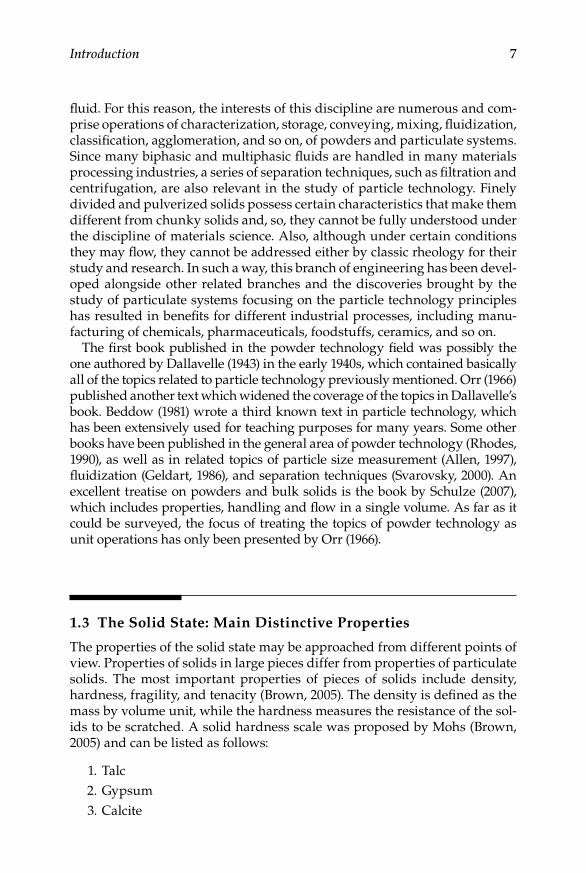
of a great deal of data. In view of this fact, consideration should be given to mechanical shape sorting before shape analysis. If shape is believed to be the cause of a particular problem or of powder behavior, then the use of sized and shaped-sorted material may provide the confirmation sought (Riley, 1968/1969; Shinohava, 1979). In some cases, however, this alternative route is not possible and, particularly in investigative work, detailed measure is nec-essary. Sebestyen (1959) suggested characterization of silhouettes by polar coordinates of their peripheries with the center of gravity of the figure as origin, as shown in Figure 1.4. When the R and θ readings are plotted, it is possible to represent the trace by a truncated harmonic series (Hatton, 1978). The value of the radius vector R as it is rotated about the origin is expressed as a function of the angle of rotation θ, in the truncated harmonic series of the form
R A A nn
n
M
n( ) cos( )θ θ ϕ= + −=
∑0
1 (1.6)
where φn is the phase angle of the nth harmonic and An = [(Bn)2 + (Cn)2]1/2. Each term of the harmonic series represents a particular shape and the silhouette is represented by different amplitudes and phases of these indi-vidual shapes (Figure 1.5). Clearly the system is not ideal because fine detail
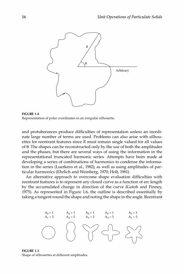
16 Unit Operations of Particulate Solids
and protuberances produce difficulties of representation unless an inordi-nate large number of terms are used. Problems can also arise with silhou-ettes for reentrant features since R must remain single valued for all values of θ. The shapes can be reconstructed only by the use of both the amplitudes and the phases, but there are several ways of using the information in the representational truncated harmonic series. Attempts have been made at developing a series of combinations of harmonics to condense the informa-tion in the series (Luerkens et al., 1982), as well as using amplitudes of par-ticular harmonics (Ehrlich and Weinberg, 1970; Holt, 1981).
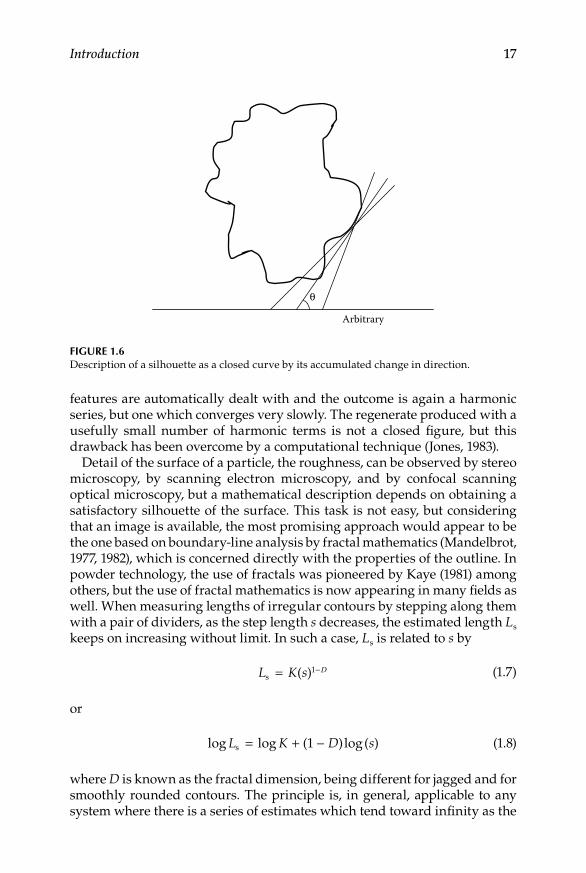
An alternative approach to overcome shape evaluation difficulties with reentrant features is to represent any closed curve as a function of arc length by the accumulated change in direction of the curve (Gotoh and Finney, 1975). As represented in Figure 1.6, the outline is described essentially by taking a tangent round the shape and noting the shape in the angle. Reentrant
A0 = 1A1 = 5
A0 = 1A2 = 5
A0 = 1A3 = 5
A0 = 1A4 = 5
A0 = 1A5 = 5
Figure 1.5Shape of silhouettes at different amplitudes.
θ
R
Arbitrary
Figure 1.4Representation of polar coordinates in an irregular silhouette.
Introduction 17
features are automatically dealt with and the outcome is again a harmonic series, but one which converges very slowly. The regenerate produced with a usefully small number of harmonic terms is not a closed figure, but this drawback has been overcome by a computational technique (Jones, 1983).
Detail of the surface of a particle, the roughness, can be observed by stereo microscopy, by scanning electron microscopy, and by confocal scanning optical microscopy, but a mathematical description depends on obtaining a satisfactory silhouette of the surface. This task is not easy, but considering that an image is available, the most promising approach would appear to be the one based on boundary-line analysis by fractal mathematics (Mandelbrot, 1977, 1982), which is concerned directly with the properties of the outline. In powder technology, the use of fractals was pioneered by Kaye (1981) among others, but the use of fractal mathematics is now appearing in many fields as well. When measuring lengths of irregular contours by stepping along them with a pair of dividers, as the step length s decreases, the estimated length Ls keeps on increasing without limit. In such a case, Ls is related to s by
L K ss = −( )1 D (1.7)
or
log log ( )log( )L K D ss = + −1 (1.8)
where D is known as the fractal dimension, being different for jagged and for smoothly rounded contours. The principle is, in general, applicable to any system where there is a series of estimates which tend toward infinity as the
Arbitrary
θ
Figure 1.6Description of a silhouette as a closed curve by its accumulated change in direction.
18 Unit Operations of Particulate Solids
resolution of the estimate improves. The emphasis is changed from the mag-nitude to the rate at which it is increasing toward infinity.
1.3.1.2 Particle Density
The density of a particle is defined as its total mass divided by its total vol-ume. It is considered quite relevant for determining other particle properties such as bulk powder structure and particle size, and so it requires careful definition (Okuyama and Kousaka, 1991). Depending on how the total vol-ume is measured, different definitions of particle density can be given the true particle density, the apparent particle density, and the effective (or aero-dynamic) particle density. Since particles usually contain cracks, flaws, hol-lows, and closed pores, it follows that all these definitions may be clearly different. The true particle density represents the mass of the particle divided by its volume excluding open and closed pores, and is the density of the solid material of which the particle is made. For pure chemical substances, organic or inorganic, this is the density quoted in reference books of physical/chemi-cal data. Since most inorganic materials consist of rigid particles, while most organic substances are normally soft, porous particles, true density of many biological powdered materials would be considerably low than those of min-eral and metallic powders. Typical non metallic minerals would have true particle densities well over 2000 kg/m3, while some metallic powders can present true densities of the order of 7000 kg/m3. The apparent particle den-sity is defined as the mass of a particle divided by its volume excluding only the open pores, and is measured by gas or liquid displacement methods such as liquid or air pycnometry. The effective particle density is referred as the mass of a particle divided by its volume including both open and closed pores. In this case, the volume is within an aerodynamic envelope as “seen” by a gas flowing past the particle and, as such, this density is of primary importance in applications involving flow round particles like in fluidiza-tion, sedimentation, or flow through packed beds.
Any of the three particle densities defined above should not be confused with bulk density of materials, which includes the voids between the par-ticles in the volume measured. The different values of particle density can be also expressed in a dimensionless form, as relative density, or specific gravity, which is simply the ratio of the density of the particle to the density of water. It is easy to determine the mass of particles accurately but difficult to evaluate their volume because they have irregular shapes and voids between them. The apparent particle density, or if the particles have no closed pores also the true density, can be measured by fluid displacement methods, that is, pycnometry, which are in common use in industry. The displacement can be carried out using either a liquid or a gas, with the gas employed normally being air. Thus, the two known techniques to deter-mine true or apparent density, when applicable, are liquid pycnometry and air pycnometry.
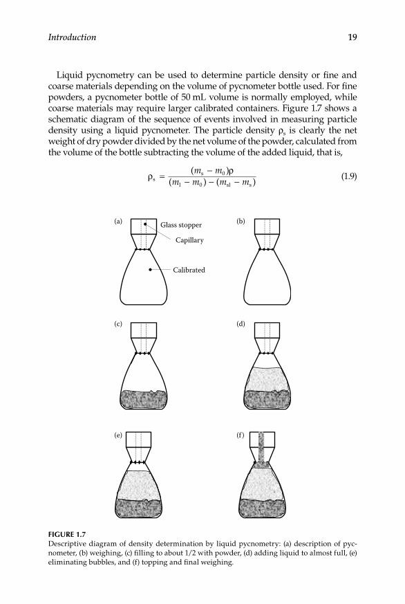
Introduction 19
Liquid pycnometry can be used to determine particle density or fine and coarse materials depending on the volume of pycnometer bottle used. For fine powders, a pycnometer bottle of 50 mL volume is normally employed, while coarse materials may require larger calibrated containers. Figure 1.7 shows a schematic diagram of the sequence of events involved in measuring particle density using a liquid pycnometer. The particle density ρs is clearly the net weight of dry powder divided by the net volume of the powder, calculated from the volume of the bottle subtracting the volume of the added liquid, that is,
ρ ρ
ss 0
l 0 sl s= ( )
( ) ( )m m
m m m m−
− − − (1.9)
Capillary
Glass stopper(a) (b)
(c) (d)
(e) (f )
Calibrated
Figure 1.7Descriptive diagram of density determination by liquid pycnometry: (a) description of pyc-nometer, (b) weighing, (c) filling to about 1/2 with powder, (d) adding liquid to almost full, (e) eliminating bubbles, and (f) topping and final weighing.

20 Unit Operations of Particulate Solids
where ms is the weight of the bottle filled with the powder, m0 is the weight of the empty bottle, ρ is the density of the liquid, ml is the weight of the bottle filled with the liquid, and msl is the weight of the bottle filled with both the solid and the liquid. Air bubbles adhering to particles and/or liquid absorbed by the particles can cause errors in density measurement. Therefore, a slowly particle absorbed liquid with low surface tension should be selected. Sometimes, when heating or boiling procedure is needed to do the gas evac-uation, the liquid that has high boiling point and does not dissolve the par-ticle should be used (Okuyama and Kousaka, 1991).
When the density of larger irregular shaped solid objects, such as com-pressed or aggregated bulk powders is needed, a method available to evalu-ate fruit or vegetable volumes might be used. A schematic diagram of a top-loading platform scale for volume and density measurement is shown in Figure 1.8. A beaker big enough to host the solid is partially filled with some kind of liquid which will not dissolve the solid. The weight of the beaker with the liquid in it is recorded and the solid object is completely immersed and suspended at the same time, using a string, so that it does not touch either the sides or bottom of the beaker. The total weight of this arrangement is recorded again, and the volume of the solid Vs can be calculated (Ma et al., 1997) by
V
m ms = −LCS LC
ρ (1.10)
where mLCS is the weight of the container with liquid and submerged solid, mLC is the weight of the container partially filled with liquid, and ρ is the density of the liquid.
Sinker rod
Liquid
Platform scale
Stand
Sample
Beaker
Figure 1.8Top-loading platform scale for density determination of irregular shaped objects.

Introduction 21
Air pycnometry can be performed in an instrument which usually consists of two cylinders and two pistons, as shown in Figure 1.9. One is a reference cylinder, which is always empty, and the other has a facility for inserting a cup with the sample powder. With no sample present, the volume in each cylinder is the same so that, if the connecting valve is closed and one of the pistons is moved, the change must be duplicated by an identical stroke in the other as to maintain the same pressure on each side of the differential pres-sure indicator. Referring to Figure 1.9, if a sample is introduced in cylinder B, and the piston in cylinder A is advanced all the way to the stop, to equalize the pressures, the measuring piston will have to be moved by a smaller distance because of the extra volume occupied by the sample. The difference in the distance covered by the two pistons, which is proportional to the sam-ple volume, can be calibrated to read directly in cubic centimeters, usually
Volume in mLSample volume
Readingscale
Valves
Measuringpiston
Referencepiston
ΔP indicator(a) (b)
(c) (d)
Stop
Cup
End Start
Pistons moving
Powder
Figure 1.9Descriptive diagram of density determination by air pycnometry: (a) description of instru-ment, (b) filling of cup, (c) pistons displacement, and (d) reading.

22 Unit Operations of Particulate Solids
with a digital counter. The method will measure the true particle density if the particles have no closed pores or the apparent particle density if there are any closed pores, because the volume measured normally excludes any open pores. If, however, the open pores are filled either by wax impregnation or by adding water, the method will also measure the envelope volume. By differ-ence between the two volumes measured the open-pore volume will be obtained, and can be used as a measure of porosity. Materials that are not surface-active and incompressible, can be measured using room air and fol-lowing the standard procedure that exposes the sample to air pressures from 1 to 2 bar. Compressible materials, however, would need to be tested at lower pressures (1/2 to 1 bar), while surface-reactive materials may be tested using helium or another inert gas, because they tend to absorb some or all of the air constituents. Considering all the aspects involved in the operation of air pyc-nometers, densities of most inorganic materials can be reliable determined using the standard procedure with normal air because their particles are normally hard and rigid.
The effective particle density is based on the average density within an aerodynamic envelope around it, including, therefore, any open or closed pores in the considered volume. One obvious way to measure the volume of the open pores is using a mercury porosimeter, but this is only suitable for coarse solids and the necessary equipment is very expensive. Alternative choices include the bed voidage method, the bed pressure drop method, and the sand displacement method. The bed voidage method (Abrahamsen and Geldart, 1980) is based on the observation that the minimum packed voidage is virtually the same for particles of similar size and particle shape. The pro-cedure consists on pouring a small amount (0.2–0.25 kg) of a control powder of known particle effective density into a measuring cylinder and tapping it to its minimum volume, corresponding to the maximum bulk density. This procedure is repeated with the unknown powder, or several control powders in an ideal context. If the porosity after tapping is assumed to be the same for the control and unknown powders, then their effective densities are in the same ratio as their bulk densities. The bed pressure method is based on mak-ing measurements of bed pressure drop as a function of gas velocity at two voidages, when gas is passed through the bed of powder in the laminar flow regime. The bed is first fluidized to get it well mixed and then gently settled to its maximum voidage. Pressure drop is measured for at least four veloci-ties; the bed is then tapped in order to reach as low voidage as possible and more measurements are made. Calling the set of measurements conditions 1 and 2 respectively, s the gradient of pressure drop, ρb the bulk density, and ρp the particle density, it can be shown (using the well-known Carman–Kozeny equation) that a basic relationship can be derived as follows:
ss
1
2
3
=
−−
ρρ
ρ ρρ ρ
b1
b2
p b2
p b1
( )( )
(1.11)

Introduction 23
where ρp is the only unknown variable and can be readily found by trial and error. The sand displacement method uses fine sand into which a known amount of coarse particles of the sample are mixed. The density of the sam-ple is determined from the difference of the bulk density of the sand alone and that of the mixture. This method is sometimes used for density determi-nations of coarse bone particles, for example, and it gives lower density than that of the solid bone as measured by pycnometry. The use of effective par-ticle density is largely restricted to fluidization and pneumatic conveying applications.
1.3.2 Packing Properties
As already stated, a powder is a complex form of solid material and it is made up of a very large number of individuals, each different from its neigh-bor. Individual, or inherent, properties have been already discussed in the previous section under the common term of primary properties. However, every time a particular powder sample is poured into a receptacle, the indi-vidual particles are located in different places from before and the structure of the powder is different. It is clear that it is not possible to predict quantita-tively how a powder will behave from a knowledge of the measured proper-ties of individual particles, and so direct measurement of bulk properties is, therefore, necessary. Because each repeated measurement on a sample will be upon a rearrangement of its population, there will be an inevitable scatter of readings. This difficulty has the consequence that the powder should be handled in as identical a manner as reasonably possible each time a mea-surement procedure is performed. Moreover, it would seem logical that there would be a development of standardized testing and characterization meth-ods, but this has not happened.
1.3.2.1 Bulk Density
The measurement of the bulk density of powders in no exception to the gen-eral situation outlined above, but it is so fundamental to their storage, pro-cessing, and distribution that it does merit particular consideration. The bulk density of a powder is its mass divided by the bulk volume it occupies. The volume includes the spaces between particles and the envelope volume of the particles themselves. The spaces between particles are denoted as poros-ity or voidage, and can be defined as the volume of the voids within the bulk volume divided by the total bulk volume. Bulk density and porosity are related by
ρ ρ ε ρ εb s g= − +( )1 (1.12)
where ρb is the powder bulk density, ρs is the particle density, ε is the poros-ity, and ρg is the gas density.

24 Unit Operations of Particulate Solids
The value of the bulk density depends on the state of the powder, particu-larly on its state of compaction. The bulk is a mixture of air (or other gas) and the solid particles, so that the bulk density can be anywhere between the density of the two phases involved. Thus, in the order of increasing bulk density, the following different definitions of this type of density that have been identified over the years are aerated bulk density, poured bulk density, tap density, and compacted bulk density. Each of these depends on the treat-ment to which the sample was subjected and, although there is a move toward standard procedures, these are far from universally adopted. There is still some confusion in the open literature in the sense of how these terms are interpreted. Some people consider the poured bulk density as loose bulk density, while others refer to it as apparent density. The actual meaning of aerated density can also be considered quite a confusing term. Strictly speak-ing, it should mean that the particles are separated from each other by a film of air and that they are, on the whole, not in direct contact with each other. Some authors, however, interpret the term as it would mean the bulk density after the powder has been aerated. Such an interpretation yields, in fact, the most loosely packed bulk density when, for cohesive materials, the strong inter-particle forces prevent the particles from rolling over each other. Considering this second interpretation, aerated and bulk densities could both be simply regarded as loose bulk density, and this approach is implied in many investigations when dealing with cohesive powders. For many fine and ultrafine powders, which are more likely cohesive in behavior, the terms more commonly used to express bulk density are loose bulk density, as poured and tapped bulk density, after vibration. Another way to express bulk density is in the form of a fraction of its particles’ solid density, which is sometimes referred as the “theoretical density.” This expression, as well as the use of porosity instead of density, enables and facilitates the unified treat-ment and meaningful comparisons of powders having considerably differ-ent particle densities.
The aerated bulk density is, in practical terms, the density when the pow-der is in its most loosely packed form. Such a form can be achieved by drop-ping a well-dispersed “cloud” of individual particles down into a measuring vessel. Alternatively, gas fluidization can sometimes be used with the gas turned slowly off and the particles allowed to settle quietly into place. The structure within the vessel is held by the cohesive forces between the parti-cles, and can be extremely fragile. Leveling off the surface of the powder at the top of the vessel is difficult to achieve without causing particle movement leading to error, as some structure collapses. Determination of aerated bulk density can be performed using an apparatus such as the one illustrated in Figure 1.10. As shown, an assembly of a screen cover, a screen, a spacer ring, and a chute is attached to a mains-operated vibrator of variable amplitude. A stationary chute is aligned with the center of a preweighed 100 mL cup. The powder is poured through a vibrating sieve and allowed to fall a fixed height of 25 cm approximately through the stationary chute into the cylindrical cup.
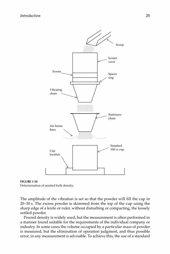
Introduction 25
The amplitude of the vibration is set so that the powder will fill the cup in 20–30 s. The excess powder is skimmed from the top of the cup using the sharp edge of a knife or ruler, without disturbing or compacting, the loosely settled powder.
Poured density is widely used, but the measurement is often performed in a manner found suitable for the requirements of the individual company or industry. In some cases the volume occupied by a particular mass of powder is measured, but the elimination of operation judgment, and thus possible error, in any measurement is advisable. To achieve this, the use of a standard
Standard100 cc cup
Scoop
Screencover
ScreenSpacerring
Vibratingchute
Stationarychute
Air-bornefines
Cuplocation
Figure 1.10Determination of aerated bulk density.

26 Unit Operations of Particulate Solids
volume and the measurement of the mass of powder to fill it are needed. Certain precautions which should be taken are clear, for example, the mea-suring vessel should be thick rather than thin, the powder should always be poured from the same height, and the possibility of bias in the filling should be made as small as possible. Although measuring of poured bulk density is far form standardized, many industries use a sawn-off funnel with a trap door or stop, to pour the powder through into the measuring container. Some decide on a standard volume, usually a measuring cylinder, to be used for the volume measurement and that varies from 50 to 1000 mL depending on the product and its size; 1 L is now accepted by many as preferred. It is also better to use a density cylinder with a 2:1 length-to-diameter ratio than the much slimmer measuring cylinder. Few people standardized the height of fall as well, realizing that the height will affect the compaction state of the powder. Finally, it is also the practice in some industries to allow the powder, after pouring it into the container, to settle to its stable density for about 10 min before scraping off the top.
The tap bulk density, as is implied by its name, is the bulk density of a powder which has been settled into a closer packing than existed in the poured state by tapping, jolting, or vibrating the measuring vessel. As with poured bulk density, the volume of a particular mass of powder may be observed, but it is generally better to measure the mass of powder in a fixed volume. Although many people in industry measure the tap density by tap-ping the sample manually, it is best to use a mechanical tapping device so that the conditions of sample preparation are more reproducible. An instru-ment useful to achieve such reproducibility is the Hosokawa powder charac-teristic tester, which has a standard cup (100 mL) and a cam-operated tapping device which moves the cup upward and drops it periodically (once in every 1.2 s). A cup extension piece has to be fitted and powder added during the sample preparation so that at no time the powder packs below the rim of the cup. After the tapping, excess powder is scraped from the rim of the cup and the bulk density is determined by weighing the cup.
The compacted bulk density would refer to the density of a powder com-pacted over and above what can be attained by tapping. There are no stan-dard procedures for determining the compacted bulk density, other than the rather specialized soil compaction tests and density determinations, quoted in a British Standard for soils (British Standards Institution, 1975).
1.3.2.2 Other Packing Properties
Compressibility can be defined as the compaction of a powder by tapping or mechanical compression. These processes can occur either unintentionally as a result of handling or transporting, or intentionally as when producing tablets or agglomerates. In the materials processing industry, unintentional compression is normally undesirable, while operations aimed at obtaining defined shapes are usually required in some processes. The former will be
Introduction 27
discussed in this section, whereas the latter will be included under the gen-eral scope of processing operations, in a subsequent part of this text.
Sone (1972) reported the following compressibility relationship, by tap-ping, for food powders:
γ n
nV VV
abnbn
= − = +0
0 1 (1.13)
where γn is the volume reduction fraction, V0 is the initial volume, Vn is the volume after n taps, and a and b are constants.
The applicability of Equation 1.13 was tested through its fit to the following linear form:
nab
nanγ = +1
(1.14)
The constant a in Equations 1.13 and 1.14 represents the asymptotic level of the volume change or, in other words, the level obtained after a large number of tappings or a long time in vibration. The constant b is representative of the rate at which this compaction is achieved, that is, 1/b is the number of vibra-tions necessary to reach half of the asymptotic change. In general, this form of data presentation is very convenient for systems comparisons since it only involves two constants.
A very common undesirable aspect of compressibility is its negative influ-ence on flowing capacity. Compression tests have been used widely in phar-maceutics, ceramics, metallurgy, civil engineering, and in the food powder field, as a simple and convenient technique to powder compressibility and flowability.
The pressure–density for powders in a compression test at low-pressure range can be described by the following equation (Barbosa-Canovas et al., 1987):
ρ σ ρρ σ( ) 0
0
− = +a b log
(1.15)
where ρ(σ) is the bulk density under the applied normal stress σ, ρ0 is the initial bulk density, and a and b are constants. The constant b represents, specifically, the compressibility of a given powder. Compression tests are useful in characterizing the flowability of powders because the interparticle forces that enable open structures in powder beds succumb under relatively low pressures. As shown in Equation 1.15, the constant b representing the change in bulk density by the applied stress is referred to as the powder compressibility. It has been found that b can be correlated with cohesion of a variety of powders and therefore could be a simple parameter to indicate
28 Unit Operations of Particulate Solids
flowability changes (Peleg, 1977). Generally, the higher the compressibility the poorer the flowability, but if quantitative information about flowability is required, shear tests are necessary (Schubert, 1987).
One of the standard methods to evaluate the flowability of a particulate system is to calculate the Hausner ratio after tapping. The Hausner ratio is defined as the ratio of a powder system’s initial (loose) bulk density to its tapped bulk density (i.e., the ratio of loose volume to tapped volume). It is easy to calculate the Hausner ratio and evaluate the flowability when the loose and tapped volumes of the test material are known. For a Hausner ratio of 1.0–1.1, the powder is classified as free flowing; 1.1–1.25, medium flowing; 1.25–1.4, difficult flowing; and >1.4, very difficult flowing (Hayes, 1987).
Adding small amounts of fine powders is often used to improve the flow properties of powdered materials in the chemical, pharmaceutical, and food industries. In this case, the fine particles coat the coarser particles of the main constituent and prevent them sticking together. Damp or sticky solids, which are difficult to handle, may be converted into free-flowing after the added fine powders absorb small quantities of liquids. Another way to improve flowability of food powders is by using the agglomeration process, which is accomplished by wetting the fine particles in an atmosphere of water or suit-able solvent droplets, causing them to collide and stick together, and then drying the agglomerated material in an air stream. Apart from improving flowability, agglomerated powders may show better wettability and dispers-ibility in liquids, and tend to be dust-free (Hoseney, 1994). Agglomeration will be discussed further in Chapter 5 of this text.
Reconstitutability is the term used to describe the rate at which dried materials pick up and absorb water reverting to a condition which resembles the undried material, when put in contact with an excessive amount of this liquid (Masters, 1976). In the case of powdered dried biological materials, a number of properties may influence the overall reconstitution characteris-tics. For instance, wettability describes the capacity of the powder particles to absorb water on their surface, thus initiating reconstitution. Such a prop-erty depends largely on particle size. Small particles, representing a large surface area-to-mass ratio, may not be wetted individually. In fact, they may clump together sharing a wetted surface layer. This layer reduces the rate at which water penetrates into the particle clump. Increasing particle size and/or agglomerating particles can reduce the incidence of clumping. The nature of the particle surface can also affect wettability. For example, the presence of free fat in the surface reduces wettability. The selective use of surface active agents, such as lecithin, can sometimes improve wettability in dried powders containing fat. Another important property is the sinkability, which describes the ability of the powder particles to sink quickly into the water. This depends mainly on the size and density of the particles. Larger, more dense particles sink more rapidly than finer, lighter ones. Particles with a high content of occluded air may be relatively large but exhibit poor sink-ability because of their low density. Finally, dispersibility describes the ease

Introduction 29
with which the powder may be distributed as single particles over the sur-face and throughout the bulk of the reconstituting water, while solubility refers to the rate and extent to which the components of the powder particles dissolve in the water. Dispersibility is reduced by clump formation and is improved when the sinkability is high, whereas solubility depends mainly on the chemical composition of the powder and its physical state.
References
Abrahamsen, A. R. and Geldart, D. 1980. Behaviour of gas fluidized beds of fine pow-der. Part I: Homogeneous expansion. Powder Technology 26: 35–46.
Allen, T. 1997. Particle Size Measurement. Vol. 1: Powder Sampling and Particle Size Measurement. London: Chapman & Hall.
Barbosa-Canovas, G. V., Málave-López, J., and Peleg, M. 1987. Density and compress-ibility of selected food powders mixture. Journal of Food Process Engineering 10: 1–19.
Beddow, J. K. 1981. Particulate Science and Technology. New York, NY: Chemical Publishing Co.
British Standards Institution. 1975. BS 1377: 1975. Methods of Tests for Soils for Civil Engineering Purposes. London: BSI.
British Standards Institution. 1993. BS 2955: 1993. Glossary of Terms Related to Particle Technology. London: BSI.
Brown, G. G. 2005. Unit Operations. Delhi: CBS Publishers & Distributors.Dallavelle, J. M. 1943. Micromeritics: The Technology of Fine Particles. New York, NY:
Pitman Publishing.Davies, R. 1984. Particle size measurement: Experimental techniques. In Handbook of
Powder Science and Technology. Fayen, M. E. and Otten, L. (eds.). New York, NY: Van Nostrand Reinhold.
Davis, G. E. 1904. A Handbook of Chemical Engineering. Manchester: Davis Bros.Ehrlich, R. and Weinberg, B. 1970. An exact method for characterization of grain
shape. Journal of Sedimentary Petrology 40: 205–212.Ennis, B. J., Green, J., and Davies R. 1994. Particle technology: The legacy of neglect in
the U.S. Chemical Engineering Progress 90: 32–43.Geldart, D. 1986. Gas Fluidization Technology. New York, NY: John Wiley & Sons.Gotoh, K. and Finney, J. L. 1975. Representation of size and shape of a single particle.
Powder Technology 12: 125–130.Green, D. W. and R. H. Perry. 2008. Perry’s Chemical Engineer’s Handbook, 8th Ed. New
York, NY: McGraw-Hill.Hayes, G. D. 1987. Food Engineering Data Handbook. New York, NY: John Wiley &
Sons.Herdan, G. 1960. Small Particle Statistics. London: Butterworths.Hoseney, R. C. 1994. Principles of Cereal Science and Technology. St. Paul, MN: American
Association of Cereal Chemists.Jones, S. 1983. The problem of closure in the Zahn–Roskies method of shape descrip-
tion. Powder Technology 34: 93–94.

30 Unit Operations of Particulate Solids
Kaye, B. H. 1981. Small Characterization of Fine Particles. New York, NY: John Wiley & Sons.
Luerkens, D. W., Beddow, J. K., and Vetter, A. F. 1982. Morphological Fourier descrip-tors. Powder Technology 31: 209–215.
Ma, L., Davis, D. C., Obaldo, L. G., and Barbosa-Canovas, G. V. 1997. Mass and spatial characterization of biological materials. In Engineering Properties of Foods and Other Biological Materials. Pullman, WA: Washington State University Publisher.
Mandelbrot, B. B. 1977. Fractals, Form, Chance and Dimension. San Francisco, CA: Freeman.
Mandelbrot, B. B. 1982. The Fractal Geometry of Nature. San Francisco, CA: Freeman.Masters K. 1976. Spray Drying Handbook. New York, NY: John Wiley & Sons.McCabe, W. L. and J. C. Smith. 1956. Unit Operations of Chemical Engineering. New
York, NY: McGraw-Hill.McGraw-Hill Dictionary of Scientific and Technical Terms, 6th Ed. 2003. New York, NY:
McGraw-Hill Professional.Okuyama, K. and Kousaka, Y. 1991. Particle density. In Powder Technology Handbook.
Iinoya, K., Gotoh, K. and Higashitani, K. (eds.). New York, NY: Marcel Dekker.Orr, C. 1966. Particulate Technology. New York, NY: Macmillan.Parfitt, G. D. and Sing, K. S. W. 1976. Characterization of Powder Surfaces. New York,
NY: Academic Press.Peleg, M. 1977. Flowability of food powders and methods for its evaluation—A
review. Journal of Food Process Engineering 1: 303–328.Rhodes, M. J. 1990. Principles of Powder Technology. New York, NY: John Wiley &
Sons.Riley, G. S. 1968/1969. An examination of the separation of differently shaped parti-
cles. Powder Technology 2: 315–319.Schubert, H. 1987. Food particle technology part I: Properties of particles and particu-
late food systems. Journal of Food Engineering 6: 1–32.Schulze, D. 2007. Powders and Bulk Solids: Behavior, Characterization, Storage and Flow.
New York, NY: Springer.Sebestyen, G. S. 1959. On Pattern Recognition with Application to Silhouettes. DSc Thesis.
Cambridge, MA: Massachusetts Institute of Technology.Shinohava, K. 1979. Mechanism of segregation of differently shaped particles in fill-
ing containers. Industrial Engineering Chemical Process Design and Development 18: 223–227.
Sone, T. 1972. Consistency of Foodstuffs. Dordrecht, The Netherlands: D. Reidel.Svarovsky, L. 2000. Solid–Liquid Separation. Oxford: Butterworth-Heinemann.Tardos, G. I. 1995. Development of a powder technology option at CCNY. Chemical
Engineering Education (Summer 1995): 172–177, 181.Valiente, A. and R. P. Stivalet, 1980. El Ingeniero Químico, ¿Qué Hace? México City:
Alahambra Mexicana.Walker, W. H., Lewis, W. K., and W. H. McAdams. 1937. Principles of Chemical
Engineering. New York, NY: McGraw-Hill.

31
2Bulk Solids: Properties and Characterization
2.1 Introductory Aspects
Taking into account all the sizes and shapes that may be found in solids, the most important from the standpoint of chemical engineering is the small particle. An understanding of the characteristics and features of minute sol-ids populations is needed for designing processes and equipment dealing with streams containing such solids. As opposed to chunk solid pieces, finely divided solids can be referred to by denominations as varied as particulate solids, pulverized solids, granular materials, and so on. In process engineer-ing literature (chemical engineering, mechanical engineering, chemistry, physics, materials science, etc.), a generic term having been used to describe a huge population of small particles forming a defined material, is simply “powder” or “industrial powder.” Powders present some characteristics so distinctive that make them practically different, by comparison, with any other state of matter. Intrinsically, molecules forming a solid piece are joined by chemical bonds and interactions stronger than those forming liquid or gases. Externally, however, there are no interactions of the chemical bond type keeping together small particles forming a powder batch. It has been suggested that the individual entities within masses of particulate solids are so kept only by geometrical accommodation. In this chapter, the most important distinctive characteristics of industrial powders are described and discussed, in the context of their importance and relevance within the discipline of Powder Technology or Particle Technology.
Some of the distinctive characteristics of powders, that have made them subject of research efforts to understand their behavior are
Powders are not solids, but may deform under compression.•Powders are not liquids, but they may flow under certain •circumstances.Powders are not gases, but they may be compressed up to a degree.•
Considering the powders’ features listed above, it becomes clear that even a definition of powder would be difficult to establish. A first approach could

32 Unit Operations of Particulate Solids
be as follows: “A powder is a group of solid particles not filling completely the space they occupy; the space not filled by particles is filled by gas.” This definition results somewhat inappropriate since nobody will call powder to a pile of rocks. In searching for a more appropriate definition, it has been observed for quite a while that dry powders possess many properties com-mon to fluids, such as exerting pressure on container vessels and flowing through channels or orifices. There are, nonetheless, important differences such as
A powder does not exert uniform pressure on all directions in con-•finement. The exerted pressure is minimal at the perpendicular direction of the applied pressure.An applied shear force on the surface of a mass of powder is trans-•mitted through all the static mass, unless a fracture occurs.The density of a mass of powder varies depending on its degree of •packaging; it increases if the powder is compacted by vibration, shaking, taping, and so on.
The above-listed characteristics originated, from the 1960s, a special focus of attention on the fluid-related properties that a powder may acquire under certain conditions. If powders would be able to follow some of the typical behavior of fluids, it would be possible to study them making use of modi-fied fluid mechanics theoretical models. A suitable manner of making a powder behave as a fluid is to suspend its individual particles within a stream of gas. When any stable suspension of solid particles of a powder in a gas stream is achieved, it is said that the powder has been fluidized. A powder that is able to be fluidized would be most properly defined as: “Disperse diphasic system in which the disperse phase consists on particles of a finely divided solid and the continuous phase consists of a gas.” The solid particles conform to a sort of mechanical network due to certain inter-particle forces. The net can be expanded under some conditions, but will reassume its packed state under the influence of gravity. The packed, station-ary state of a mass of powder presents mechanical resistance and some degree of elasticity. The interaction particle–gas is fundamental, and deter-mines primarily the flowing capacity of the powder.
2.2 Classification of Powders
The different ways of classifying powders is closely related to the applications in which bulk properties play an important role. Since most applications in powder technology are relevant when considering powders as dispersion sys-tems, they can be classified into different categories according to their particular

Bulk Solids 33
behavior in dynamic situations. For this reason, powders or dry particulate materials can be categorized according to their handling properties. The clas-sification depends on the type of handling in question, with the cases of deaerated state and aerated state being most important. The classification of powders in the deaerated state is known as Jenike’s classification, while the classification of powders in the aerated state is called Geldart’s classification.
2.2.1 Jenike’s Classification
In the deaerated state, powders can be classified using a shear cell tester or a compression tackiness tester. A precise definition of the flowability of a pow-der is only possible with several number of curves derived from a family of yield loci of the powder, measured with a shear cell. There are several designs of shear cells that are also used to measure other properties of powders, and so they will be discussed in detail in a further section, but basically they measure different shearing forces for corresponding normal forces on con-solidated powder samples. The curve representing the relation between the maximum shear and normal stresses is called the yield locus. Each yield locus also gives one pair of values for the unconfined yield stress σc and major consolidation stress σ1. The ratio of the consolidation stress to the unconfined yield strength is called the flow factor ff. Jenike (1964) proposed a classification according to the position of one point of the failure function at a fixed value of the unconfined yield stress with respect to the flow factor line. Figure 2.1 shows a schematic representation of classification of powders following this criterion. As can be seen, at a fixed value of the unconfined yield strength of 22.3 N, the straight lines through the origin at a slope 1/ff would represent the categories of very cohesive, cohesive, easy flowing, and
Cohesive
ff = 10ff = 2 ff = 4(22N)
Verycohesive
Easyflowing
Freeflowing
σ1
σc
Figure 2.1Graphical representation of classification of powders according to Jenike.

34 Unit Operations of Particulate Solids
free flowing, as represented in the mentioned figure, as well as in Table 2.1. In addition to Jenike’s classification, Williams et al. (1970/1971) has also defined simple powders as those whose failure function is a straight line through the origin, providing that the slope of the line is less than 1/ff.
Another way of classifying powders is on the basis of the results obtained with a compression tackiness tester. This tester is a simplified version of the uniaxial compression test, on a cylindrical briquette of the powder, where the compression force at failure is a direct measure of the powder tackiness. The consolidation stresses used to form this briquette are generally greater than those used with the Jenike shear test. The total compression force is supposed to simulate pressures greater than that of the bottom of a 180 cm high pile of bags in storage. Tackiness values above 27 N usually indicate powders that can cause problems due to their sticky characteristics and the shape of a curve of tackiness value against initial compression load is also an indication of tackiness: nontacky powders give essentially a horizontal line while tacky products show the effect of increasing compression.
2.2.2 geldart’s Classification
With regard to the aerated state, a widely accepted classification of powders is the one proposed by Geldart (1973), which takes the two most important particle properties into account: particle size and particle density. Geldart’s classification is basically derived from the behavior of powders when fluid-izing by air at ambient conditions. In the fluidizing state, a bed of powder starts expanding when the fluidizing air reaches a critical velocity known as minimum fluidizing velocity. Considering the different ways of powders in expansion, Geldart suggested four types of powders. Figure 2.2 illustrates the four general manners in which different powders behave when subjected to these described conditions of fluidization. According to such figure, pow-ders can be termed as A, B, C, and D type and may be described as follows. A powders are sometimes referred to as slightly cohesive or catalyst type and exhibit large bed expansion after minimum fluidization and before ini-tiation of bubbling. The air velocity at which bubbling begins is known as the minimum bubbling velocity. Increasing this velocity will increase num-ber and size of bubbles. B powders are known as sand like and present
Table 2.1
Classification of Powders According to Jenike
Type of Powder ff Value at σc = 22.3 N
Very cohesive Less than 2Cohesive Between 2 and 4Easy flow Between 4 and 10Free flow More than 10

Bulk Solids 35
bubbling at the minimum fluidization velocity with a small bed expansion. In this type of powders the minimum fluidizing velocity equals the mini-mum bubbling velocity so that bubbles appear immediately with bed expan-sion. This bed expansion is said to be due to bubbling only. C powders are called cohesive and are difficult to fluidize at all. When the minimum expan-sion velocity is surpassed, these powders do not expand or form bubbles. The air is released through cracks forming irregular channel paths within their mass volume. They do not show any kind of expansion because the pressure drop through the bed is considerably lower than its weight over the cross-sectional area. D powders are simply known as large and can form stable spouted beds if the air is admitted only through a centrally positioned hole. Over the minimum fluidizing velocity these powders form large bub-bles, which burst when reaching the surface so that air is released and spout-ing is observed. Geldart’s classification can also be represented in a plot of particle fluid density difference versus particle size, as shown in Figure 2.3. As can be observed, D powders are extremely large to even be considered powders. It has been observed that their behavior is determined exclusively by hydrodynamics and that interparticle forces do not play a role.
The above-mentioned classification of powders may be useful even when fluidization as such is not of interest. For example, in the filling of containers and in the residence time needed in hoppers to avoid flooding out when the discharge valve is opened, the bed expansion and the rate of deaeration are of concern. There is a striking difference between A, B, and C powders in the way they behave in deaeration: A-type powders collapse at a constant rate, B-type powders deaerate almost instantaneously, while C-type powders col-lapse initially much faster than those in group A but may remain in a slightly aerated state for a considerable period, with the pressure at the bottom of the bed decaying very slowly. The deaeration rate can, therefore, also be used to characterize powders, but Geldart and Wong (1985) found this to be insuffi-ciently sensitive and developed a standardized deaeration time test.
A B C D
Figure 2.2Behavior of powder beds when fluidized.

36 Unit Operations of Particulate Solids
Geldart’s classification has been well accepted by powder technologists since its release. Some powders, however, may present behavior variations when certain conditions may change. For example, an A powder could show the behavior of a B powder if effective gravity would increase by using a gas with viscosity lower than air viscosity. Rietema et al. (1980) have suggested a generic classification by using dimensionless groups, which takes into account important variables such as cohesion, gas viscosity, and acceleration due to gravity. According to this approach, dimensionless groups may be used to represent the behavior limit between powders A and B, as well as between powders A and C. This approach does not consider, as previously mentioned, D systems of particles as powders. For the limit of behavior of powders A and B, theoretical principles discussed elsewhere (Rietema and Mutsers, 1973; Mutsers and Rietema, 1977) have shown that homogeneous bed expansion is possible when
Fl < −
−
150(1 )(3 2 )
2εε ε2
(2.1)
where Fl is the fluidization number and ε is the porosity or voidage of the bed.
The limit of behavior between A and B powders is, therefore, represented by
Fl = −
−
150(1 )(3 2 )
2εε ε2
(2.2)
Mean particle size (μm)100 1000
1
10
C
Cohesive
A
Catalyst
B
Sand-like
D
LargePa
rtic
le-fl
uid
dens
ity d
iffer
ence
(g/c
m3 )
Figure 2.3Graphical representation of classification of powders according to Geldart.

Bulk Solids 37
In terms of the limit of behavior between A and C powders, a dimensionless Group known as cohesion number Coh, is defined as
Coh
s= C
x g( )( )ρ (2.3)
where C is a constant known as the constant of powder cohesion, ρs is the powder density, x is an equivalent diameter of the particle, and g is the accel-eration due to gravity.
In the compacted (or consolidated) state the elasticity module of a powder has a value approximately equal to the value the cohesion constant. The flu-idization number for a powder at its consolidated state can be, therefore, modified as
Fl s
3
g2*4 2
=ρ x g
Cµ
(2.4)
where Fl* is the fluidization number for consolidated powders, and μg is the gas viscosity.
Equation 2.4 is, actually, the product of the inverse of the cohesion number and another dimensionless group known as the Archimedes number Ar, and thus
Fl Ar(Coh)* 1= − (2.5)
The Archimedes number Ar is defined as
Ar s
2 3
g=
ρµx g
(2.6)
When values of Coh versus Ar are plotted, the resulting graph will show the behavior limits of powders A and B and powders A and C, as represented in Figure 2.4. As can be observed, the behavior limits of powders A and B are function of the bed voidage.
2.3 Sampling
Sampling is an important element of powder handling that demands careful scientific design and operation of the sampling systems. The general pur-pose of sampling is to collect a manageable mass of material which must be

38 Unit Operations of Particulate Solids
representative of the total mass of the sampled powder. This action is achieved by taking many small samples from all parts of the total which, when combined, will represent this total with an acceptable degree of accu-racy. All particles in the total must have the same probability of being included in the final sample, so all of them must be equally accessible. To satisfy these requirements, the following basic “golden rules” of sampling should be applied whenever possible:
Sampling should be done preferably from a moving stream (for both •powders and suspensions) but powder on a stopped belt can be sampled.A sample of the whole of the stream should be taken for many •(equally spaced) periods of time, rather than part of the stream for the whole of the time.
The first rule recommends that the sample should be taken from flowing powder stream, such as discharging from a belt conveyor or a feeding flow from one storage container to another. Also, as the second rule mentions, the sampling process should continue for a long series of short time intervals (Masuda, 1997). It is very likely that the recombined, primary sample taken
103
104
105
106
100101
Geldart’s powder B
Geldart’spowder C
Geldart’s powder A
0.350.400.450.50
ε
Cohesion number (Coh)
Arc
him
edes
num
ber (
Ar)
Figure 2.4Dimensionless representation of Geldart’s classification for powders A, B, and C.

Bulk Solids 39
from the whole will be too large for most powders tests. It will be, therefore, necessary to subdivide the original sample into secondary, or even tertiary, subsamples. This subdivision may be built into the primary sampler or it may be achieved with a separate sampling divider.
If a sampled material is perfectly homogeneous with respect to its proper-ties, any fraction of the bulk would be exactly the same as far as those prop-erties are concerned. For instance, if a certain powder is heterogeneous on size but homogeneous on density, it would be considered homogeneous if it is sampled to determine density. This is the reason why it is often eas-ier to obtain a representative sample from liquid materials, where all their properties are, generally, homogeneous. For example, when sampling ionic solutions for component concentration, any variation in results would be normally attributed to experimental error. However, when the material is heterogeneous, as it virtually happens with industrial powders, it is expected to find difference in some measured properties. The source of these varia-tions, in addition to variations caused by the assaying process, could be attributed to the fact that the smaller fragments of particulate material are themselves heterogeneous and to segregation of certain types of fragments due to handling of the bulk material (Gy, 1982). The probability of obtaining a perfect unbiased sample from the parent material is remote. If several sam-ples are taken and they are representative, the expected variation may be estimated from statistical analysis (Allen, 1981).
The statistical theory of sampling considers a sample of size N (N speci-mens) selected randomly and independently. A random selection process must be such that every member of the population being sampled would have the same chance to be selected. The independency of specimens implies that the selection of one specimen does not influence the selection of another in the whole mass of the sampled powder. These requirements are not usu-ally met in practice, either due to the two sources of variations previously mentioned or to the nature of the sampling technique, or both. For example, a perfectly blended batch of a binary mixture of powders may become segre-gated during the sampling process due to the nature of the mechanical han-dling system. The act of sampling can be considered a process that allows observing the realizations of a random variable whose statistical properties are determined by the inherent characteristics of the sampled population and the sampling process. Naturally, the apparent variability of the deter-mined values can be greatly influenced by the sampling and measurement techniques. In statistics, a random variable is defined as a function which assigns real numbers to the outcomes of a random experiment. For particu-late materials, the random experiment consists of: the selection of a fraction of a given volume of bulk by giving equal chance to all other fractions in the lot, further reduction of volume and selection of a fraction of the specimen for testing, and testing of a final fraction for different properties. The ran-dom variable being observed is defined by the sampling process. A change in the volume of the specimen in the sampling process will correspond to a
40 Unit Operations of Particulate Solids
different experiment, and so it will result in the realization of a different random variable. When sampling from a well-mixed bulk of particulate material, it can be postulated that the random variables observed by choos-ing different specimen volumes would possess the same distribution func-tion and the same mean, but different variances. The theoretical and experimental studies indicate that, keeping other things constant, reduction of specimen volume increases the variance. A practical relationship has been proposed by Gy (1982), which is useful in determining the minimum accept-able specimen weight as a function of the diameter of the coarsest fraction in the total mass of sampled powder. Such relationship can be represented as
M
Cxs
3
≥σ2
(2.7)
where σ2 is the variance of the tolerated sampling error, C is a constant char-acterizing the material to be sampled, x is the diameter of the coarsest frag-ment, and Ms is the weight of the specimen.
The arithmetic average of random independent observations of a normally distributed random variable is known to be the best estimator of the unknown population mean. The Central Limit Theorem (Kennedy and Neville, 1986) asserts that the arithmetic average of random independent observations of a random variable will be distributed normally when the sample size is infi-nitely large. Even for moderately sample sizes, the statistical behavior if the sample average is acceptably close to that of the Normal distribution. Also, by increasing the number of specimens (sample size), sample averages closer to the unknown value of the population mean are obtained. The Law of Large Numbers (Larson, 1995) establishes that when the sample size is infi-nitely large, the sample mean becomes equal to the population mean. In practice, however, small sample amounts are handled for obvious practical and economic reasons, and so it is practically impossible for the sample aver-age to become equal to the unknown population mean. For this reason, it is used to establish an interval around the sample average, called a confidence interval, which will contain the unknown mean with a certain predeter-mined probability. Given the probability (1–α), the length of the confidence interval becomes a function of the population variance and the sample size. This relationship is derived from the following probability statement:
Prob (1- ) (1- )X Z
N
X Z
N
−≤ ≤
+
= −α ασ
µσ
α/ /2 2 1
(2.8)
where X is the sample arithmetic average, σ is the population standard deviation, μ is the population mean and N is the sample size, and Z(1–α)/2 is the (1–α)/2 percentile of standard Normal variable.
Bulk Solids 41
The length L of the confidence interval is
L
Z
N= −2 2(1 )α σ/
(2.9)
It is clear from Equation 2.9 that the length of the confidence interval is lin-early proportional to the population standard deviation, and inversely related to the square root of the sample size. If σ were known, Equation 2.9 could be used to determine the minimum sample size required to obtain a confidence interval which will contain the unknown mean μ, with a (1–α) probability. An expression for the minimum sample size will, therefore, be
N
ZL
≥ −4 22
2(1 )2
α σ/
(2.10)
Since σ is usually unknown and the sampling process has normally the aim of estimating the standard deviation as well as the mean, Equation 2.10 has limited applicability but indicates, however, an important relationship between the sample size, the inherent variability of the sampled population, and the precision at which the mean μ is to be estimated. Such precision will be increased by reducing L and/or increasing (1–α), both resulting in larger sample sizes. Also, as indicated by the power of σ in Equation 2.10, its vari-ability will increase the sample size quadratically. Reduction of σ is only possible by employing a different sampling method, further crushing or grinding the bulk to be sampled, or increasing the specimen volume. Considering that all these measures are not very practical for real purposes, an alternative would be the use of an estimator for σ, which is a well-known practice in statistics. A relationship for estimating the population standard deviation can be represented as follows:
S
NX Xi
i
N2 2
1
11
= − −=∑ ( )
(2.11)
where S is the estimator for σ, and Xi is the assay value.Since the variance is not known, but estimated by S, the following proba-
bility statement can be established:
Prob (1 ) (1 )X t S
N
X t S
NN N−
≤ ≤+
= −− − − −α α α/ , / ,2 1 2 1 1µ
(2.12)
where S is the sample standard deviation, and t(1–α)/(2, N−1) is the (1–α)/2 per-centile of the Student’s t distribution with N–1 degrees of freedom.
42 Unit Operations of Particulate Solids
The length of the confidence interval can be expressed by
L
t S
NN= − −2 2 1(1 )α / ,
(2.13)
An expression for the minimum sample size can be derived from Equation 2.13, similarly to the one derived from Equation 2.11, that is,
N
t SL
N≥ − −4 2 12 2
2(1 )α / ,
(2.14)
By inspecting Equations 2.11 and 2.14, it can be noticed that the values of S and t are not independent of N. Also, a sample of a certain size is needed, for example, N’, to obtain S initially. This value will change as new specimens are sampled, assayed, and their values used in recalculating S. When the population variance is unknown, it is not possible to determine exactly the minimum sample size. An approach can be achieved by taking several sam-ples and calculating successive approximations of N. To accomplish this, using a small sample size the estimator S is determined by means of Equation 2.11 and a new value for N is calculated with appropriate values of t(1–α)/(2, N−1), S, and L using Equation 2.11. If this value is larger than the actual sample size, additional sampling is done and the procedure repeated. As the sample size increases the value of S will approach the unknown population standard deviation with decreasing error. However, the successive values of S as sample size increases may fluctuate around σ with decreasing error and, thus, the calculated values of N will also fluctuate. For this reason, it is advis-able to increase the sample size by smallest possible increments, and con-tinually calculate N until its value and the actual sample size are sufficiently close.
A practical approximation can be done considering the ratio L2/S2 in Equation 2.14 and estimating the population mean for a given confidence interval, such that its length be equal to a certain multiple of S. In such a manner, an initial determination of the sample size is possible. By rearrang-ing terms in Equation 2.14, the following relationship can be obtained:
U
tN
N≥ − −4 2 12(1 )α / ,
(2.15)
where U = L2/S2.Equation 2.15 can be used to calculate different values of U determined
by certain values of α and N. The value of the percentiles of Student’s t distribution, are available in most of the standard textbooks on statistics. The results of such calculations for different confidence levels can be pre-sented in graphical or tabular form. Table 2.2 lists U values for sample

Bulk Solids 43
sizes from 2 to 500 for confidence levels of 0.90, 0.95, and 0.99. It can be used to read directly the required minimum sample size for a predetermined value of U. Table 2.2 shows that, in agreement with probability principles, as the confidence interval length L shortens with respect to the estimator of the standard deviation S, the unknown mean and standard deviation
Table 2.2
Sample Size as a Function of U
U = L2/S2
Sample Size N 1–α = 0.90 1–α = 0.95 1–α = 0.99
2 79.63 323.09 8105.193 11.37 24.65 131.214 5.52 10.11 34.115 3.63 6.18 16.936 2.69 4.40 10.837 2.15 3.43 7.878 1.81 2.78 6.139 1.54 2.37 5.0210 1.34 2.04 4.2311 1.19 1.81 3.6512 1.08 1.61 3.2213 0.97 1.46 2.8814 0.90 1.33 2.5915 0.83 1.22 2.3716 0.77 1.13 2.1817 0.72 1.06 1.8918 0.67 0.99 1.7719 0.63 0.93 1.6620 0.60 0.87 1.6421 0.56 0.83 1.5422 0.54 0.79 1.4623 0.51 0.75 1.3824 0.49 0.71 1.3225 0.47 0.68 1.2526 0.45 0.65 1.2027 0.43 0.63 1.1428 0.41 0.60 1.1029 0.40 0.58 1.0530 0.39 0.55 1.0240 0.28 0.41 0.7350 0.22 0.32 0.5760 0.19 0.27 0.4780 0.14 0.20 0.35100 0.11 0.16 0.28200 0.05 0.08 0.14500 0.02 0.03 0.05
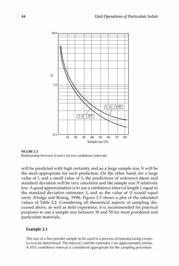
44 Unit Operations of Particulate Solids
will be predicted with high certainty and so a large sample size N will be the most appropriate for such prediction. On the other hand, for a large value of L and a small value of S, the predictions of unknown mean and standard deviation will be very uncertain and the sample size N relatively low. A good approximation is to use a confidence interval length L equal to the standard deviation estimator S, and so the value of U would equal unity (Dodge and Romig, 1998). Figure 2.5 shows a plot of the tabulated values of Table 2.2. Considering all theoretical aspects of sampling dis-cussed above, as well as field experience, it is recommended for practical purposes to use a sample size between 30 and 50 for most powdered and particulate materials.
example 2.1
The size of a fine powder sample to be used in a process of manufacturing ceram-ics is to be determined. The interval L and the estimator S are approximately similar. A 95% confidence interval is considered appropriate for the sampling procedure.
10 20 30 40 50 60 70 80Sample size (N)
0.1
1.0
10.0
U
1–α = 0.95
1–α = 0.9
Figure 2.5Relationship between U and L for two confidence intervals.

Bulk Solids 45
SoluTion
Since L and S are approximate equal, the value of U (L2/S2) will approach unity. Consequently, the interception of U = 1 with the curve for 1–α = 0.95 in Figure 2.5 will read the value of 18 directly. Alternatively, reading from Table 2.2 for U = 0.99 and 1–α = 0.95, the size sample is 18.
Sampling methods are normally designed or selected for collection of primary samples from large-scale processes. In many applications, samplers have to be designed specifically for a particular material and duty. Usually, there are two main stages in any sampling scheme. A gross sample, which represents the parent batch, is initially collected and, then, a representative laboratory sample is prepared from this gross sample. These two operations are generally per-formed by different techniques. Gross samples can range up to 50 kg or more, depending of the size of the bulk quantity, while laboratory samples rarely exceed 1 or 2 kg, or even less considering the wide array of state-of-the-art instrumental methods currently available for powder characterization. This small amount of sample may require further subdivision, as to use an appro-priate number of specimens determined by the minimum sample size previ-ously discussed.
Segregation is one of the main troubles encountered in the sampling of solid particles. In conical heaps of material, for instance, a large proportion of the coarser particles will generally be found in the lower levels of the pile. On the other hand, coarse particles tend to migrate toward the top of the contents of a container, especially after transportation. Any selected sampling method must take into account these irregularities. Grab sampling with scoops or shovels is considered a common alternative for obtaining bulk samples. A large number of random samples may be taken from a heap of the material, or regular sam-ples (e.g., every nth shovelful) can be scooped into a sample container when the bulk material is transported manually from one location to another. Regular sampling is most often favored for materials packed in containers. A common sampling implement for this purpose is a piece of metal tubing with a sharp bottom edge and fixed to a long handle, known as sampling “thief.” This sam-pler is pushed gently, firmly, and vertically into the full depth of the material, and then withdrawn for sample removal. When sampling from stored powders the samples have to be withdrawn from small spaces of equal volume within the total, in an effort to try to give a chance to every member of the population to be sampled. Since this is very difficult to achieve as not all of the material is equally accessible, sampling from stationary places is generally to be avoided.
For material flowing down chutes or from hoppers, a sample collector may be placed in the path of the outlet stream. Open-ended scoops or shovels are unsuitable in this case because they allow coarser particles to roll out of the sample and thus bias the sample toward the finer fractions. A ladle is the only recommended device for such sampling (Plowman, 1985) since it does not allow this rolling out to happen, unless overfilled. The falling stream is traversed with the laden to collect the sample, and if the whole of the stream

46 Unit Operations of Particulate Solids
cannot be sampled in one pass, it is divided into several equal areas with the sample being collected from those incrementally. In agreement with the golden rules of sampling mentioned before, the collector should sample the whole of the outflow stream at regular time intervals.
Stopped belt sampling is considered the best manual sampling method. It is often taken as a reference method with others being compared against it. It follows the two golden rules of sampling in that it samples from a moving stream (with the movement momentarily stopped for taking the sample) and it takes the whole of the stream many times. It is carried out with a suitable profiled sampling frame which is inserted through the material on a stopped belt conveyor until it comes in contact with the conveyor belt over its full width. The material within the frame is then collected from the belt and it represents one increment in the manual sampling series.
At the laboratory level, gross samples can be subdivided into one or more smaller samples manually or mechanically. The most common manual method is the one known as “coning and quartering,” which consists in mix-ing the sample and pile it into a conical heap, flatten it about one quarter of its original height, divide the flatten heap into four equal quarters, and reject two opposite quarters while remixing the remaining pair. This remaining amount is piled again into a new heap, and the procedure is repeated until the required sample quantity is obtained. As mentioned before, sampling methods have sometimes to be designed for specific purposes. Also, the many stages of a sampling scheme often required, makes sampling a tech-nique which has to be carried out very carefully, and taking many samples is normally involved in the whole process.
Sample dividers are used to reduce the size of the primary sample and can be classified as intermittent and reciprocating cutters, as well as continuous and rotational dividers. The rotational dividers are usually considered more suitable than linear cutters. A common type of divider, shown in Figure 2.6, is a box with an open top divided into a number of compartments with their bottoms sloping toward opposite sides of the box. When a quantity of mate-rial is poured evenly into the hopper, it is split into equal portions. Thus, by successive repetitions of the procedure, the sample can be reduced to the minimum amount required to perform an assay. An alternative to reduce a sample to a given proportion in a single step can be performed with a sample reducer, such as the one illustrated in Figure 2.7. As can be seen, by pouring the sample through the hopper at the top of the inclined plane, a fixed reduc-tion of the whole amount of sample can be obtained. A very efficient sample divider is the spinning riffler (Allen and Khan, 1970), which follows quite well both golden rules of sampling. As can be seen in Figure 2.8, such sam-pling splitter comprises a hopper mounted above a vibratory feeder, and a rotating carousel divided into many compartments. In operation, the sample is slowly conveyed from the hopper by the feeder onto sampling containers fixed to the compartments. The subsamples are collected into such contain-ers, and the feed rate is controlled by varying the gap under the hopper, as

Bulk Solids 47
Figure 2.6Sample divider or chute sample splitter.
Figure 2.7Diagram of a sample reducer.
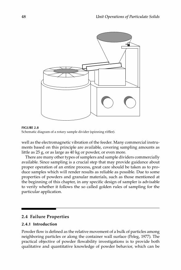
48 Unit Operations of Particulate Solids
well as the electromagnetic vibration of the feeder. Many commercial instru-ments based on this principle are available, covering sampling amounts as little as 25 g, or as large as 40 kg or powder, or even more.
There are many other types of samplers and sample dividers commercially available. Since sampling is a crucial step that may provide guidance about proper operation of an entire process, great care should be taken as to pro-duce samples which will render results as reliable as possible. Due to some properties of powders and granular materials, such as those mentioned at the beginning of this chapter, in any specific design of sampler is advisable to verify whether it follows the so called golden rules of sampling for the particular application.
2.4 Failure Properties
2.4.1 introduction
Powder flow is defined as the relative movement of a bulk of particles among neighboring particles or along the container wall surface (Peleg, 1977). The practical objective of powder flowability investigations is to provide both qualitative and quantitative knowledge of powder behavior, which can be
Figure 2.8Schematic diagram of a rotary sample divider (spinning riffler).

Bulk Solids 49
used in equipment design and in equipment performance prediction (Sutton, 1976). The flow characteristics of powders are of great importance in many problems encountered in bulk material handling processes in diverse types of industries, such as the agricultural, ceramic, chemical, food, mineral, min-ing, and pharmaceutical industries, because the ease of powder conveying, blending, and packaging depends on them (Chen, 1994). Practically, for all fine and very fine powders, the attractive forces between particles are large when compared with the weight of individual particles and so they are said to be cohesive and normally present flow problems. For example, such mate-rials can fail to flow out of a container in which there is a hole, thousand of times larger than the diameter of the particle. To guarantee steady and reli-able flow, it is crucial to accurately characterize the flow behavior of powders. The forces involved in powder flow are gravity, friction, cohesion (interpar-ticle attraction), and adhesion (particle-wall attraction). The first requirement is to identify the properties which characterize the flowability of a particular material and to specify procedures for measuring them. The common belief that the flowability of a powder is a direct function of the angle of the repose is misleading and should be avoided because, as stated earlier, most indus-trial powders show different grades of cohesiveness. The angle of repose of a cohesive material is indeterminate, being dependent on the previous story of a given sample, and is irrelevant to the flow behavior of the material in any particular situation. The behavior of the material depends on the manner in which its strength varies with its state of compaction. For example, a slightly cohesive powder may be able to flow and be poured through a hole (forming a pile with a slope equal to the angle of repose), but after being compressed by simple tapping the flow would not develop due to the formation of a sta-ble cohesive arch over the hole. A very small change in the bulk density of the powder would have, therefore, caused a dramatic change in its flowabil-ity. The important feature of a particulate material is the way its shear strength varies with the consolidating stress, and the properties used to identify and quantify such interactions are commonly known as the failure properties of a powder.
The requirement for getting powders to flow is for their strength to be less than the load put on them, that is, they must fail. The basic properties describing this condition are known as “failure properties” and they are the following: (a) the effective angle of internal friction, (b) the angle of wall friction, (c) the failure function, (d) the cohesion, and (e) the ultimate tensile strength. The failure properties take into account the state of compaction of the powder as this strongly affects its flowability unless the powder is cohe-sionless, like dry sand, and it gains no strength on compression. The time of consolidation can also have an effect on failure properties of powders. It is, therefore, important to test such properties under controlled conditions using sealed powder samples or air-conditioned rooms or enclosures. Also, time-consolidating samples must be tested to simulate storage conditions.
50 Unit Operations of Particulate Solids
2.4.2 Description of Failure Properties
The effective angle of internal friction δ is a measure of the friction between particles and depends on their size, shape, roughness, and hardness. The angle of wall friction ϕ is equivalent to the angle of friction between two solid surfaces except that one of the two surfaces is a powder. It describes the friction between the powder and the material of construction used to confine the powder, for example, a hopper wall. The wall friction causes some of the weight to be supported by the walls of a hopper. The failure function FF is a graph showing the relationship between unconfined yield stress (or the strength of a free surface of the powder) and the consolidating stress, and gives the strength of the cohesive material in the surface of an arch as a func-tion of the stress under which the arch was formed. The cohesion C is, as mentioned earlier, is a function of interparticle attraction and is due to the effect of internal forces within the bulk that tend to prevent planar sliding of one internal surface of particles upon another. The ultimate tensile strength T of a powder compact is the most fundamental strength mechanism, repre-senting the minimum force required to cause separation of the bulk struc-ture without major complications of particle disturbances within the plane of failure.
There are several ways, direct or indirect, of testing the five failure proper-ties defined above. Basically, all of them can be determined using a shear cell, but simplified or alternative procedures can be adopted when the aim is to monitor the flowability of the output from a process or compare a number of materials.
2.4.3 experimental Determinations
There are basically three types of shear cells available for powder testing: (a) the Jenike shear cell, also known as the translational shear box; (b) the annu-lar or ring shear cell, also called the rotational shear box; and (c) the rota-tional shear cell, which is a fixture of a powder rheometer.
The Jenike shear cell is circular in cross section, with an internal diameter of 95 mm. A vertical cross section through the cell is shown in Figure 2.9. It consists of a base, a ring which can slide horizontally over the base, and a cover. The Jenike test sequence simulates the changes in stresses acting on an element of materials flowing through bin. The ring and base are filled with the powder and a lid is placed in position. By means of a weight carrier, which hangs from a point at the center of the lid, a vertical compacting load can be applied to the powder sample. The lid carries a bracket with a project-ing pin and a measured horizontal force is applied to such bracket, causing the ring and its content, as well as the lid, to move forward at a constant speed. The procedure to carry out a test on a powder consists of three steps: preconsolidation to ensure uniformity of samples, consolidation to repro-duce flow with a given stress under steady-state conditions, and shearing to

Bulk Solids 51
measure shear stress at failure. The preconsolidation consists in filling the assembly of base, ring and a packing mold ring over it, with a sample pow-der. A twisting top is placed on the sample and a force is applied to the top while giving it a number of oscillating twists. The force is released, the twist-ing top removed, and the powder surface is carefully scraped level with the upper half of the cell. In the consolidation step a shear cover is placed over the powder sample and a selected normal force is applied on it. A shear force is then continuously applied until it reaches a steady-state value indicating plastic flow. The shear force is then interrupted and the stem retracted. The shearing step comprises replacing the normal force of consolidation by a smaller force and reapplying the shearing force until the stress/strain peaks and falls off indicating failure plane in the sample and a point in the yield locus. The procedure is repeated with five or six different vertical loads, pro-gressively smaller, applied to a set of identical samples and the shear force needed to initiate flow is found in each case. The forces are divided by the cross-sectional area of the cell to give stresses and the shear stress is plotted against the normal stress. The resulting graph is a yield locus (Figure 2.10), and it is a line that gives the stress conditions needed to produce flow for the powder when compacted to a fixed bulk density.
If the material being tested is cohesive, the yield locus is not a straight line and does not pass through the origin. It can be shown that the graph when extrapolated downward cuts the horizontal axis normally. As shown in Figure 2.10, the intercept T is the tensile strength of the powder compacts
τ
W1
Lid
Ring
Base
Powder(a)
(b) W0
Consolidation Shear
Figure 2.9Diagram of Jenike’s shear cell.

52 Unit Operations of Particulate Solids
tested and the intercept C is called the cohesion of the powder; the yield locus ends at the point A. The yield locus represents the results of a series of tests on samples which have the initial bulk density. More yield loci can be obtained by changing the sample preparation procedure and, in this way a family of yield loci can be obtained (Figure 2.11). This family of yield loci contains all the information needed to characterize the flowability of a par-ticular material; it is not, however, in a convenient form. For many powders, yield locus curves can be described by the empirical Warren–Spring equa-tion (Chasseray, 1994):
τ σC T
n
= + 1
(2.16)
Shea
r str
ess (τ)
Normal stress (σ)
Figure 2.11A family of yield loci.
T Normal stress (σ)
Shea
r str
ess (τ)
A
C
Figure 2.10The Jenike yield locus.

Bulk Solids 53
where τ is the shear stress, C the material’s cohesion, σ the normal stress, T the tensile stress, and n the shear index (1 < n < 2).
Apart from the cohesion and the tensile stress, the effective angle of inter-nal friction can also be determined using the yield locus derived from test-ing a particular powder in a shear cell. The effective angle of internal friction is the resulting angle from drawing a tangent line to the Mohr circle inscribed in the yield locus, and passing through the origin (as shown in Figure 2.12).
The angle of wall friction can be measured by replacing the base of a Jenike shear cell by a plate of the material of which the hopper (or any sort of con-tainer) is to be made. The ring from the shear cell is placed on the plate and filled with powder and the lid is put in position. The shear force needed to maintain uniform displacement of the ring is found for different vertical loads on the lid. The slope of the graph of shear force against normal force gives the angle of friction between the particles and the wall, or angle of wall friction. This measure would complete the testing of a particulate material using only a Jenike shear cell.
The Jenike shear cell has been considered for long time the testing cell for establishing standard procedures in industrial applications and research. It has been recognized as one of the standards for testing bulk solids in the United States and in Europe, being especially focused on cohesive powders. The complexity of this method is such that errors due to poor technique can easily arise. A reference material has therefore been produced with which laboratories can verify both their equipment and experimental technique. The reference material consists of 3 kg of limestone powder packed in a poly-ethylene jar. It is accompanied by a certificate giving shear stress as a func-tion of normal applied stress for four different powder compaction stresses.
δ
Mohr circle
Normal stress, σ
Shea
r str
ess, τ
Figure 2.12Graphical determination of the effective angle of internal friction.
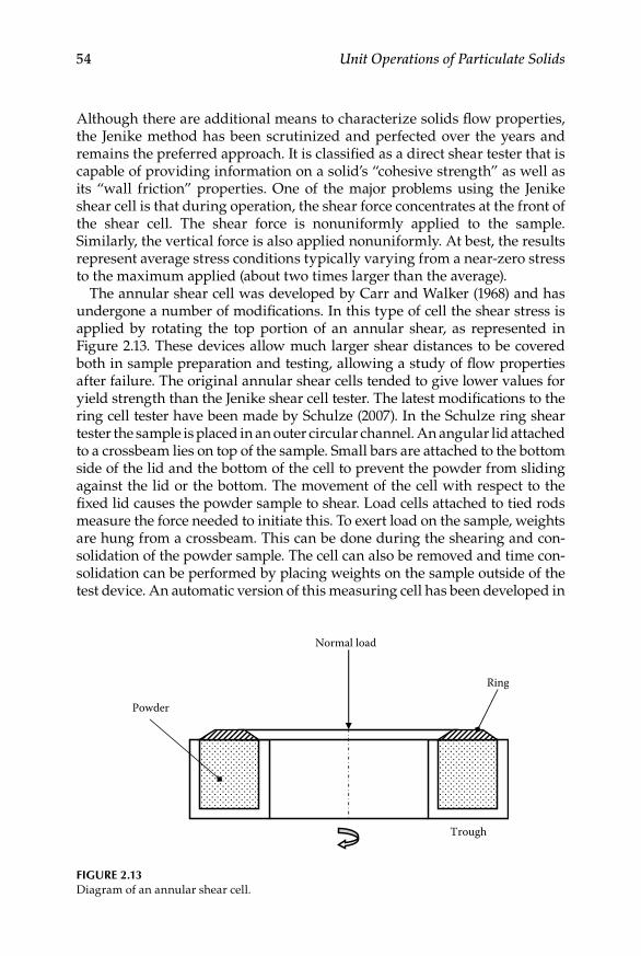
54 Unit Operations of Particulate Solids
Although there are additional means to characterize solids flow properties, the Jenike method has been scrutinized and perfected over the years and remains the preferred approach. It is classified as a direct shear tester that is capable of providing information on a solid’s “cohesive strength” as well as its “wall friction” properties. One of the major problems using the Jenike shear cell is that during operation, the shear force concentrates at the front of the shear cell. The shear force is nonuniformly applied to the sample. Similarly, the vertical force is also applied nonuniformly. At best, the results represent average stress conditions typically varying from a near-zero stress to the maximum applied (about two times larger than the average).
The annular shear cell was developed by Carr and Walker (1968) and has undergone a number of modifications. In this type of cell the shear stress is applied by rotating the top portion of an annular shear, as represented in Figure 2.13. These devices allow much larger shear distances to be covered both in sample preparation and testing, allowing a study of flow properties after failure. The original annular shear cells tended to give lower values for yield strength than the Jenike shear cell tester. The latest modifications to the ring cell tester have been made by Schulze (2007). In the Schulze ring shear tester the sample is placed in an outer circular channel. An angular lid attached to a crossbeam lies on top of the sample. Small bars are attached to the bottom side of the lid and the bottom of the cell to prevent the powder from sliding against the lid or the bottom. The movement of the cell with respect to the fixed lid causes the powder sample to shear. Load cells attached to tied rods measure the force needed to initiate this. To exert load on the sample, weights are hung from a crossbeam. This can be done during the shearing and con-solidation of the powder sample. The cell can also be removed and time con-solidation can be performed by placing weights on the sample outside of the test device. An automatic version of this measuring cell has been developed in
Ring
Trough
Normal load
Powder
Figure 2.13Diagram of an annular shear cell.

Bulk Solids 55
which a computer can automatically add loading to the sample and condition it. The instrument can be operated in a manual, semiautomatic, or totally automatic mode. Both, the original shear cells or the latest modified ones offer several important advantages over the Jenike-type shear cell. The area of shear is constant while the handling is easier, because consolidation and shear are quicker. After the sample is consolidated, a full locus can be generated with-out need of reconsolidating after each load. The consolidation process becomes more automated and uniform, eliminating much of the operator variability in the measurement process, characteristic of the Jenike-type tester.
Rotational shear cells, or powder rheometers, are relatively new testing instruments that can sensitively measure how flowability changes under a wide range of processing conditions, including various speeds, levels of entrapped air, and degrees of attrition. Powder rheometers also can condition the sample before testing, reducing the variability produced by differences in storage and handling. These instruments automatically rotate a blade through a cylindrical column of powder measuring the energy or force it needs to move through the sample and relating these measurements to vari-ous characteristics of the powder. The powder is placed in a circular vessel with a closed bottom. The blade is introduced into the powder and moves downward or upward in a helical motion, while the force on the blade shaft is recorded. The helical path along which the blade moves is dependant on the axial and rotational speeds, as well as in the direction of the blade rota-tion. The angle of approach the blade makes with the powder can be varied, so that the direction and angle of the measurement will allow one to measure compaction, shear, and slicing of the powder sample within the vessel. The torque data are treated to determine the largest theoretical torque exerted by the whole powder column on the rotor blade for any defined test condition. Therefore, powder shear can be measured under different shear conditions, including various downward compaction modes and upward expansion modes. The blade is interchangeable and different designs are used for dif-ferent needs, including a rotating shear cell that can be used in a shallow column of powder. An arrangement as this is shown in Figure 2.14, and is called an open shear cell. As can be observed, the operations of this cell would be analogous to a rotational viscometer used in characterizing highly consistent non-Newtonian fluids. In congruence with this analogy, the open shear cell will measure both the force and the torque, and so these variables could be related to the shear stress and the normal stress to obtain the yield locus of a powder. Satisfactory results using rotational shear cells have been reported in different applications and with diverse industrial powders (Freeman and Cook, 2006; Freeman et al., 2009). Powder rheometers can pro-vide simple and sensitive testing as they are relatively operator independent and yield quantitative values.
The angle of internal friction can be measured directly by the “grooved plate” method. The base of the Jenike shear cell is replaced by a metal plate in which a number of saw-toothed grooves are cut (Figure 2.15). These
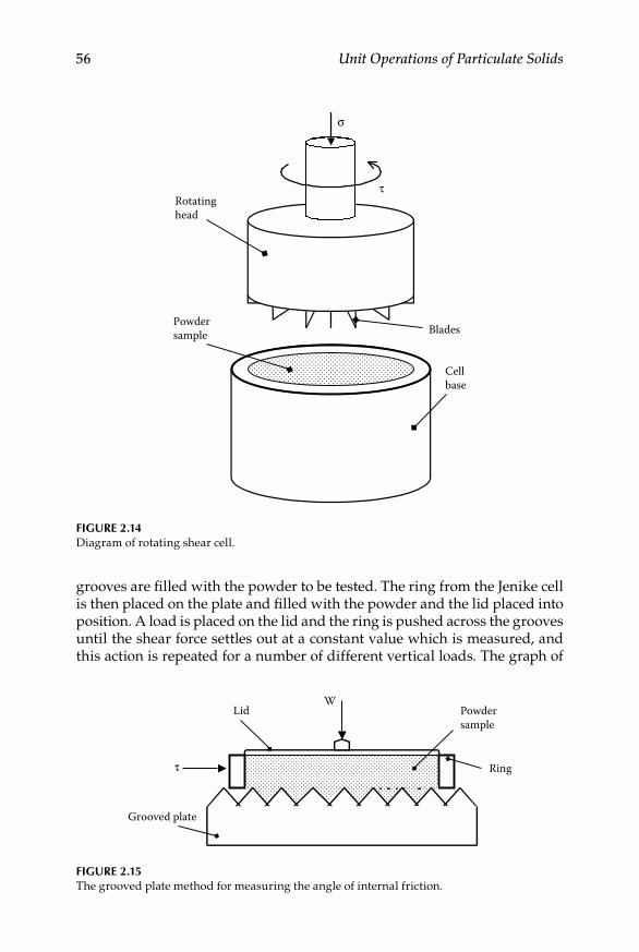
56 Unit Operations of Particulate Solids
grooves are filled with the powder to be tested. The ring from the Jenike cell is then placed on the plate and filled with the powder and the lid placed into position. A load is placed on the lid and the ring is pushed across the grooves until the shear force settles out at a constant value which is measured, and this action is repeated for a number of different vertical loads. The graph of
Grooved plate
W
τ
Lid
Ring
Powdersample
Figure 2.15The grooved plate method for measuring the angle of internal friction.
τ
σ
Blades
Rotatinghead
Powdersample
Cellbase
Figure 2.14Diagram of rotating shear cell.

Bulk Solids 57
shear force against normal force will be a straight line with its slope being the angle of internal friction of the powder.
For direct measurement of the failure function a split cylindrical die as shown in Figure 2.16 is used. The bore of the cylinder may conveniently be about 50 mm and its height should be just more than twice the bore. The cylinder is clamped so that the two halves cannot separate and it is filled with the powder to be tested, which is then scraped off level with the top face. By means of a plunger the specimen is subjected to a known consoli-dating stress. The plunger is then removed and the two halves of the split die are separated, leaving a free standing cylinder of the compacted pow-der. A plate is then placed on top of the specimen and an increasing vertical load is applied to it until the column collapses. The stress at which this occurs is the unconfined yield stress, that is, the stress that has to be applied to the free vertical surface on the column to cause failure. If this is repeated for a number of different compacting loads and the unconfined yield stress is plotted against the compacting stress, the failure function of the powder will be obtained.
A graph of a failure function of a powder is given in Figure 2.17. Although the results of this method can be used for monitoring or for comparison,
Figure 2.16Device for direct measurement of failure function.

58 Unit Operations of Particulate Solids
the failure function obtained will not be the same as that given by shear cell tests, due to the effect of die wall friction when forming the compact. A method of correcting for friction has been described by Williams et al. (1971). They proposed to compact the powder in a series of short incre-ments and extrapolate results to estimate the unconfined yield stress for an infinite number of increments, that is, for a uniformly consolidated pow-der. Figure 2.18 shows a schematic diagram of the apparatus devised for the corrected method described. The cylinder is sectioned, not only into two halves, but also into 13 horizontal segments. The lower section at the base is 25.4 mm high, while the remaining 12 are half as high as this (12.7 mm high). The effect of the relationship length–diameter, used to adjust the values of the indirect method, is best evaluated using a single section at a time, that is, repeating the method of the complete cylinder section by section.
Two methods can be used for direct measurement of tensile strength. In the first, a mould of the same diameter as the Jenike cell is split across its diameter. The base of the cell is roughened by sticking sandpaper to it. The two halves are clamped together, the cell is filled with the powder, and then a lid is placed in position. The specimen is compacted by the application of a known vertical force to the lid and this, along with the clamp, is removed. The two halves of the cell, containing the specimen, rest on a base plate in which slots have been cut to form an air bearing. Air is introduced so that the cell can move horizontally without friction and the force needed to pull the two halves of the specimen are determined (Hong and Watanabe, 2000). Knowing the cross-sectional area of the specimen the tensile strength can be found. Measurements are made for a number of compacting loads and
Consolidation stress, σ1
Unc
onfin
ed yi
eld
stre
ss, σ
c
Figure 2.17Failure function of a powder.

Bulk Solids 59
Figure 2.18Scheme of the device for measuring a corrected failure function.

60 Unit Operations of Particulate Solids
tensile strength is plotted against compacting stress. This method is quite difficult to perform properly, requiring careful attention to details. The sec-ond method is easier to use and gives results with less scatter. In this case a mould of the same diameter as the Jenike shear cell, and a lid which just fits inside it, are used. The base of the cell and the lower face of the lid are cov-ered with sticking tape on which glue is spread. The cell is filled with the powder which is scraped off level with the top of the cell and the lid is placed in position. A compacting load is applied to the lid by means of a weight hanger and left in position until the glue has hardened. The lid is then attached through a tensile load cell to an electric motor, by which the lid is slowly lifted. The stress required to break the specimen is thus obtained. After failure, the lid and the base of the cell are examined and the result is accepted only if both are completely covered with powder, showing that tensile failure has occurred within the powder specimen and not at the surface. Figure 2.19 presents a diagram of these two methods for direct mea-suring of tensile strength.
The two methods described above for measuring the tensile strength of a lightly compacted powder do not give the same results, providing evidence that a bed of a particulate material will generally not be isotropic (i.e., its properties, including tensile strength, will be different in different direc-tions). Since the second method is easier to use, while the compacting stress
a1
(a)
(b)
a2
b1 b2
Figure 2.19Methods for measuring tensile strength: (a) horizontal split cell, (b) lifting lid cell.
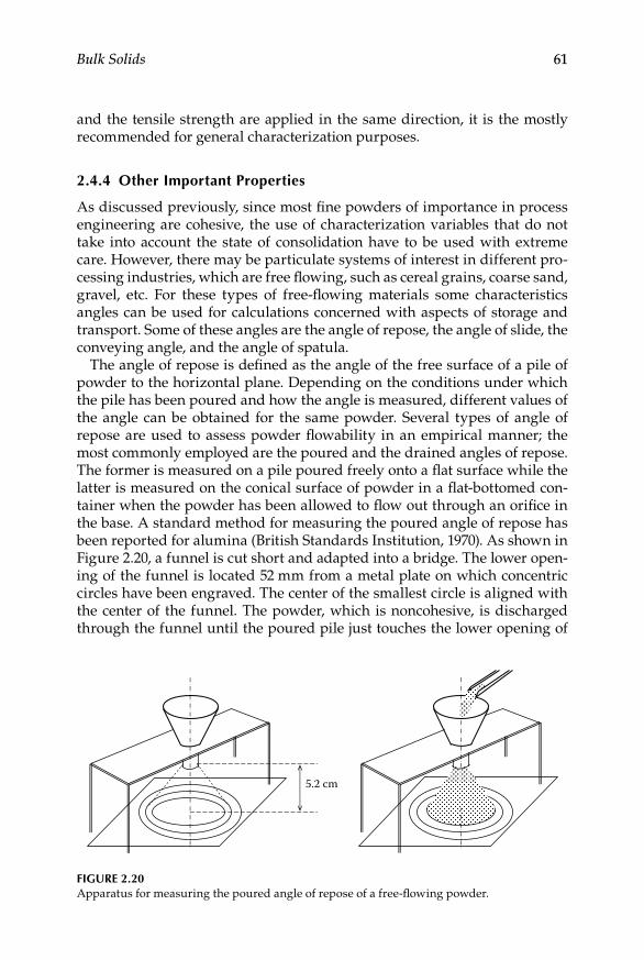
Bulk Solids 61
and the tensile strength are applied in the same direction, it is the mostly recommended for general characterization purposes.
2.4.4 other important Properties
As discussed previously, since most fine powders of importance in process engineering are cohesive, the use of characterization variables that do not take into account the state of consolidation have to be used with extreme care. However, there may be particulate systems of interest in different pro-cessing industries, which are free flowing, such as cereal grains, coarse sand, gravel, etc. For these types of free-flowing materials some characteristics angles can be used for calculations concerned with aspects of storage and transport. Some of these angles are the angle of repose, the angle of slide, the conveying angle, and the angle of spatula.
The angle of repose is defined as the angle of the free surface of a pile of powder to the horizontal plane. Depending on the conditions under which the pile has been poured and how the angle is measured, different values of the angle can be obtained for the same powder. Several types of angle of repose are used to assess powder flowability in an empirical manner; the most commonly employed are the poured and the drained angles of repose. The former is measured on a pile poured freely onto a flat surface while the latter is measured on the conical surface of powder in a flat-bottomed con-tainer when the powder has been allowed to flow out through an orifice in the base. A standard method for measuring the poured angle of repose has been reported for alumina (British Standards Institution, 1970). As shown in Figure 2.20, a funnel is cut short and adapted into a bridge. The lower open-ing of the funnel is located 52 mm from a metal plate on which concentric circles have been engraved. The center of the smallest circle is aligned with the center of the funnel. The powder, which is noncohesive, is discharged through the funnel until the poured pile just touches the lower opening of
5.2 cm
Figure 2.20Apparatus for measuring the poured angle of repose of a free-flowing powder.

62 Unit Operations of Particulate Solids
the funnel. The concentric circles help in measuring easily the diameter of the poured pile and, since the height is fixed, by simple trigonometry the angle of repose is determined. Although, as mentioned, the method was developed for alumina, there is no reason why it may be applied for any other noncohesive, easily flowing, or free-flowing particulate system.
The drained angle of repose is always greater than the poured angle of repose, because in the first case the powder sliding or rolling down the slope is separating, while in the second it is converging. Although, as has been already discussed, the angle of repose could be considered meaningless in many practical applications, it can be used as a rough flowability indicator (Geldart et al., 1990). According to Carr (1976) angles of up to 35° indicate free flowability, angles of 35–45° indicate some cohesiveness, angles of 45–55° indicate cohesiveness (loss of free flowability), and angles 55° and above indicate very high cohesiveness and, therefore, very limited (or none) flowability.
The angle of slide is closely related to the drained angle of repose (Wilkinson et al., 1983). It is the minimum angle to the horizontal of a flat, inclined, surface that will allow bulk solid to flow from rest under its own weight. This angle is supposed to be useful in designing stationary chutes but its measurement has not been described as standardized. The value measured is expected to be highly influenced by the material of construction of the chute, the amount of material on it, and by humidity. It has been shown (Augenstein and Hogg, 1978) that the motion of individual particles strongly depends on the nature of the surface over which they flow: highly rough-ened surfaces cause shear within the flowing stream while smooth ones cause slip at the surface.
The conveying angle, also called the maximum angle of rise, is the angle at which a smooth belt conveyor can operate without the bulk powder running back down. There is a need for a standard test method to be developed for determination of this angle, to allow designers of belt conveying systems to have a reliable design criterion. A rough guide given in the literature (Wilkinson et al., 1983) establishes that the angle of rise used in such systems should not exceed about half the poured angle of repose.
The angle of spatula is measured by spooning out powder with a 22 mm wide flat-blade spatula that is inserted into the bulk powder parallel to the bottom of the container (Carr, 1965). The spatula is lifted straight up and out of the powder, keeping it parallel to a horizontal plane. The spatula is vibrated or tapped in a specified manner and the angle of the tangent to the powder surface at the edge of the spatula is measured, to the horizontal plane. The average angle of several measures is taken and, except for very free-flowing materials, its value is always greater than that of the poured angle of repose, since it is taken from a consolidated material. The angle of spatula is consid-ered useful as a very simple and rough estimate of flowability; a value under 40° indicates that the material is free flowing.
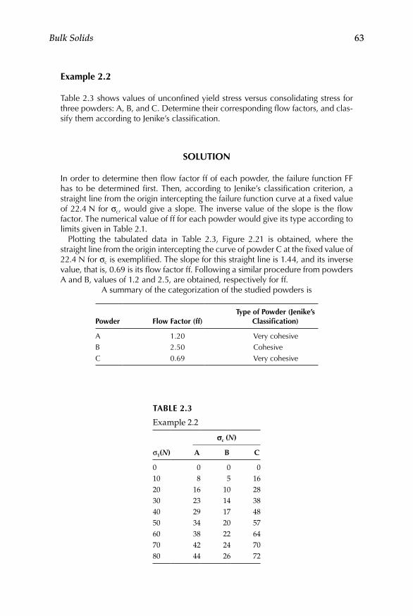
Bulk Solids 63
example 2.2
Table 2.3 shows values of unconfined yield stress versus consolidating stress for three powders: A, B, and C. Determine their corresponding flow factors, and clas-sify them according to Jenike’s classification.
SoluTion
In order to determine then flow factor ff of each powder, the failure function FF has to be determined first. Then, according to Jenike’s classification criterion, a straight line from the origin intercepting the failure function curve at a fixed value of 22.4 N for σc, would give a slope. The inverse value of the slope is the flow factor. The numerical value of ff for each powder would give its type according to limits given in Table 2.1.
Plotting the tabulated data in Table 2.3, Figure 2.21 is obtained, where the straight line from the origin intercepting the curve of powder C at the fixed value of 22.4 N for σc is exemplified. The slope for this straight line is 1.44, and its inverse value, that is, 0.69 is its flow factor ff. Following a similar procedure from powders A and B, values of 1.2 and 2.5, are obtained, respectively for ff.
A summary of the categorization of the studied powders is
Powder Flow Factor (ff)Type of Powder (Jenike’s
Classification)
A 1.20 Very cohesiveB 2.50 CohesiveC 0.69 Very cohesive
Table 2.3
Example 2.2
σc (N)
σ1(N) A B C
0 0 0 010 8 5 1620 16 10 2830 23 14 3840 29 17 4850 34 20 5760 38 22 6470 42 24 7080 44 26 72

64 Unit Operations of Particulate Solids
example 2.3
A powder is characterized running an experiment in a Jenike’s shear cell. The results are given in Table 2.4. Determine the failure properties that can be derived from the yield locus of the powder.
SoluTion
According to discussion presented in Sections 2.4.2 and 2.4.3, the failure proper-ties that can be read off directly from a yield locus are the cohesion C and the ultimate tensile strength T (Figure 2.10). Also, by drawing a Mohr circle and follow-ing the procedure described to modify the yield locus as illustrated in Figure 2.12,
Table 2.4
Example 2.3
τ (kPa) σ (kPa)
0.75 0.41.05 0.91.30 1.41.50 2.01.55 2.4
0
10
20
30
40
50
60
70
80
90
0 10 20 30 40 50 60 70 80 90
ABC
m = 1.44
σ1 (N)
σ c (N
)
Figure 2.21Graph for Example 2.2.
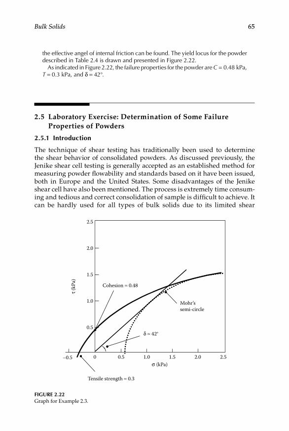
Bulk Solids 65
the effective angel of internal friction can be found. The yield locus for the powder described in Table 2.4 is drawn and presented in Figure 2.22.
As indicated in Figure 2.22, the failure properties for the powder are C = 0.48 kPa, T = 0.3 kPa, and δ = 42°.
2.5 Laboratory Exercise: Determination of Some Failure Properties of Powders
2.5.1 introduction
The technique of shear testing has traditionally been used to determine the shear behavior of consolidated powders. As discussed previously, the Jenike shear cell testing is generally accepted as an established method for measuring powder flowability and standards based on it have been issued, both in Europe and the United States. Some disadvantages of the Jenike shear cell have also been mentioned. The process is extremely time consum-ing and tedious and correct consolidation of sample is difficult to achieve. It can be hardly used for all types of bulk solids due to its limited shear
2.5
2.0
1.5
1.0
τ (kP
a)
δ ≈ 42°
σ (kPa)
Cohesion ≈ 0.48
Tensile strength ≈ 0.3
0
0.5
Mohr’ssemi-circle
–0.5 0.5 1.0 1.5 2.0 2.5
Figure 2.22Graph for Example 2.3.

66 Unit Operations of Particulate Solids
displacement, which is at most twice the thickness of the upper ring. Some bulk solids need a greater shear displacement to reach steady-state flow con-ditions. Perhaps the two critical practical disadvantages of the Jenike shear cell are its operator skillful dependence, and the extremely long time taken to perform a test under some specific conditions. Teunou and Fitzpatrick (2000) reported on an experimental stage of a project to take eight months to complete using one consolidating bench.
Alternatives to the Jenike shear cell are the annular shear cell and the rotational shear cell, also called the powder rheometer. It has been reported (Freeman and Cooke, 2006) that powder rheometers are reliable, fast, and give results comparable to standard methods based on the Jenike shear cell. The objective of the exercise is to compare the standard Jenike method for limestone CRM 116 powder with a method using a powder rheometer.
2.5.2 instrument and Materials
A rotational shear cell instrument, such as the FT4® Powder Rheometer, equipped with a 48 mm rotational shear cell and a 30 mL shear measure-ment vessel. A batch of reference limestone powder (CRM 116), produced and sold by the Commission of European Communities.
2.5.3 Shear Tester operation
Follow the directions given in the instrument manual for shear testing methodology. The routine procedure can be summarized as follows:
Condition the sample using the test blade slicing downward through •the powder followed by an upward traverse to lift the powder and drops it over the blade. This process helps to remove the effect of different sampling methodologies and powder storage times.Compact the sample by using a ventilated compaction piston (allow-•ing entrained air to escape), with a force equal to that of the preshear normal stress.Shear the sample continuously until a steady-state flow is achieved, •to complete the preshearing state.Reduced the normal stress, so that the sample is now over consoli-•dated with respect to the normal stress now applied. Restart shear-ing and measure the point of incipient failure.For each preshear normal stress, take five measurements at the five •normal stresses defined by the standard. Take also a measurement of shear stress at the preshear normal stress level, that is, at 3, 6, 9, and 15 kPa.The five measurements taken make up the yield loci for each pre-•shear normal stress level.

Bulk Solids 67
2.5.4 Calculations and report
Obtain the yield loci by plotting shear stress versus normal stress at •the different preshear normal stresses.Draw Mohr’s circles on the graphs of the yield loci derived, to extra-•polate the failure properties, such as the effective angle of internal friction. Determine the remaining failure properties that can be read from the graph.Perform a search to obtain the standard yield loci from Jenike’s test-•ing on CRM 116 limestone powder, in order to compare the results obtained with such standard.Present a complete written report, according to scientific report guide-•lines, either given by instructor or consulted in the literature. Include graphs, charts, and calculations carried out, as well as discussion on own data. Compare and discuss, as much as possible, agreements or discrepancies based on literature survey from studies and investiga-tions on the subject.
2.6 Particle Size Analysis
2.6.1 introduction
Particle size distribution measurement is a common method in any physical, mechanical, or chemical process because it is directly related to material behavior and/or physical properties of products. The bulk density, com-pressibility, and flowability of an industrial powder are highly dependent on particle size and its distribution. Segregation will take place in a free-flowing powder mixture because of the differences in particle sizes. There are many other properties of particulate systems that strongly depend on particle size, for example, activity of drugs, setting time of cement, and hid-ing power of pigments. Characterization of solid particles, which are in practice mostly irregular in shape, is usually done by analyzing particle size and its distribution. Other characteristic properties of the solid material may be included in the type of size measured; for example, Stoke’s diameter combines size, density, and shape all in one parameter. Quantitative mea-sure of particle shape can be obtained indirectly by analyzing two or more types of particle size and looking at different “shape coefficients” that relate to those sizes. There are many different types of instruments available for measuring particle size distribution but most of them would fall into four general methods: sieving, microscope counting techniques, sedimentation, and stream scanning.
68 Unit Operations of Particulate Solids
2.6.2 Definitions of Characteristic linear Dimension
In particle size measurement two most important decisions have to be made before a technique is to be selected for the analysis; these are concerned with the two variables measured, the type of particle size and the occurrence of such size. An irregular particle can be described by a number of sizes depend-ing on dimension or property is measured. Particle size was previously discussed in Chapter 1 and definitions of equivalent sphere diameters, equiv-alent circle diameters, and statistical diameters have been provided (Tables 1.2, 1.3, and 1.4). Emphasizing what was already presented, is important to bear in mind that great care must be taken when making a selection of par-ticle size, as an equivalent diameter, in order to choose the most relevant to the property or process which is to be controlled. For example, in solid–liquid separations where particle motion relative to the fluid is the governing mechanism for separation (gravity or centrifugal sedimentation, hydrocy-clones) it is of course most relevant to use a method that measures the free-falling diameter or, more often, the Stoke’s diameter. In filtration, on the other hand, it is the surface-volume diameter (measured, e.g., by permeametry), which is more relevant to the principle of separation in question.
The occurrence of amount of particle matter which belongs to specified size classes may be classified or arranged by diverse criteria as to obtain tables or graphs. In powder technology the use of graphs is convenient and customary for a number of reasons which will be mentioned and discussed as this topic is developed. For example, a particular size which is to be used as the main reference of a given material is easily read from a specific type of plot.
2.6.3 Types of Distributions
There are four different particle size distributions for a given particulate material, depending on the quantity measured: by number fN(x), by length fL(x), by surface fS(x), and by mass (or volume) fM(x). From all these, the second mentioned is not used in practice as the length of a particle by itself is not a complete definition of its dimensions. These distributions are related but conversions from one another is possible only in cases when the shape factor is constant, that is, when the particle shape is independent of the particle size. The following relationships show the basis of such conversions:
f x k x f xL N( ) ( )= ⋅ ⋅1 (2.17)
f x k x f xS N( ) ( )= ⋅ ⋅22
(2.18)
f x k x f xM N( ) ( )= ⋅ ⋅33
(2.19)
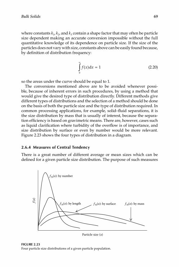
Bulk Solids 69
where constants k1, k2, and k3 contain a shape factor that may often be particle size dependent making an accurate conversion impossible without the full quantitative knowledge of its dependence on particle size. If the size of the particles does not vary with size, constants above can be easily found because, by definition of distribution frequency:
f x x( )d =
∞
∫ 10
(2.20)
so the areas under the curve should be equal to 1.The conversions mentioned above are to be avoided whenever possi-
ble, because of inherent errors in such procedures, by using a method that would give the desired type of distribution directly. Different methods give different types of distributions and the selection of a method should be done on the basis of both the particle size and the type of distribution required. In common processing applications, for example, solid–fluid separations, it is the size distribution by mass that is usually of interest, because the separa-tion efficiency is based on gravimetric means. There are, however, cases such as liquid clarification where turbidity of the overflow is of importance, and size distribution by surface or even by number would be more relevant. Figure 2.23 shows the four types of distribution in a diagram.
2.6.4 Measures of Central Tendency
There is a great number of different average or mean sizes which can be defined for a given particle size distribution. The purpose of such measures
f N(x): by surface f N(x): by massf N(x): by length
f N(x): by number
f(x)
Particle size (x)
Figure 2.23Four particle size distributions of a given particle population.
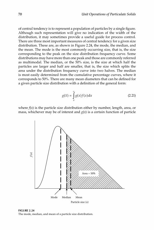
70 Unit Operations of Particulate Solids
of central tendency is to represent a population of particles by a single figure. Although such representation will give no indication of the width of the distribution, it may sometimes provide a useful guide for process control. There are three most important measures of central tendency for a given size distribution. These are, as shown in Figure 2.24, the mode, the median, and the mean. The mode is the most commonly occurring size, that is, the size corresponding to the peak on the size distribution frequency curve. Some distributions may have more than one peak and those are commonly referred as multimodal. The median, or the 50% size, is the size at which half the particles are larger and half are smaller, that is, the size which splits the area under the distribution frequency curve into two halves. The median is most easily determined from the cumulative percentage curves, where it corresponds to 50%. There are many mean diameters that can be defined for a given particle size distribution with a definition of the general form:
g x g x f x x( ) ( ) ( )=
∞
∫ d0
(2.21)
where f(x) is the particle size distribution either by number, length, area, or mass, whichever may be of interest and g(x) is a certain function of particle
Area = 50%
Mode Median MeanParticle size (x)
f(x)
Figure 2.24The mode, median, and mean of a particle size distribution.

Bulk Solids 71
size x, and depending on the form of this function there are different mean diameters x as listed in Table 2.5.
Evaluation of the various means required for a given particle size distribu-tion is based on Equation 2.21, which may also be written as
g x g x F( ) ( )= ∫ d
0
1
(2.22)
because
f x
Fx
( ) = dd
(2.23)
If either f(x) or F(x) are available as analytical functions, the desired mean diameters are evaluated by integration following Equation 2.21. If, how-ever, no analytical function is fitted and the particle size distribution is in a form of a graph or a table, evaluation of mean diameters can best be done graphically. Most particle size measurement techniques result in cumulative percentage F(x) and, thus, according to Equation 2.23 if F(x) is plotted against g(x) for a number of corresponding sizes, g(x) is then represented by the area under the curve with respect to the F(x) axis, as illustrated in Figure 2.25. The mean is evaluated from this area using the corresponding relation for g(x), as given in Table 2.5, being immaterial whether F(x) is plotted as percentage oversize or undersize. It is always best to represent a population of particles by the actual size distribution curve and only in cases when this is not pos-sible or feasible, resort to using a single number, a measure of central ten-dency, for characterizing a particulate system. In such cases, care must be taken to select the type of mean size most relevant to the given application.
2.6.5 Presentation of Data
The common way of presenting particle size data of different powders is in form of a plot. Normally, the particle size axis is the “x” or horizontal and
Table 2.5
Mean Diameters as a Function of g(x)
Form of g(x) Name of Mean Diameter, x
g(x) = x Arithmetic mean, xa
g(x) = x2 Quadratic mean, xq
g(x) = x3 Cubic mean, xc
g(x) = log x Geometric mean, xg
g(x) = 1/x Harmonic mean, xh

72 Unit Operations of Particulate Solids
the particle amount axis is the “y” or vertical. What is plotted on the par-ticle size axis is a matter of which quantity used to represent size of indi-vidual particles suits better to a specific problem. The amount of particle matter, which belongs to specified size classes on the particle axis, may also be represented in several ways. Number of particles and mass of par-ticles are the most common ones, but surface area and volume are used as well. In general, particle size distributions can be presented as frequencies f(x) or cumulative frequencies F(x), which are related to each other by the following equation:
f x
F xx
( )( )= d
d (2.24)
The graphical representation of a particle size distribution is usually plot-ted in a cumulative form. In a typical cumulative plot, points are entered showing the amount of particulate material contributed by particles below or above a specified size. Hence, the curve presents a continuously rising or decreasing character. These oversize and undersize distributions, as illus-trated in Figure 2.26, are simply related by
F x F x( ) ( )oversize undersize= −1 (2.25)
A cumulative plot will, therefore, include a broad range of particle sizes. It is often convenient, however, to refer to a single characteristic size for the system. Many characteristic sizes have been proposed, most of them
Area = g (x)
g (x)
F(x)
Figure 2.25Evaluation of a mean xa from the cumulative percentage F(x).

Bulk Solids 73
involving a mathematical formula. An important one, which can be read off any cumulative plot of the particle size data, is the median particle size. It is defined as that particle size for which the particle amount equals 50% of the total. If the particle amount is represented by number, such point is called the number median size. If mass is used as the measure of particle amount, this variable is known as the mass median size. The distinction between number and mass median is very important, since they differ generally by a consider-able amount. Such difference means that number and mass cumulative plots do not agree for the same system of particles. The weight of a particle, which varies as the cube of its diameter, account for this mentioned disagreement. For practical purposes, it is reasonable to fit an analytical function to experi-mental particle size distribution data, and then handle this function mathe-matically in further treatment. It is, for example, very much easier to evaluate mean sizes from analytical functions than from experimental data. Several different distribution functions can be found in the literature. All of them should be treated as empirical equations as they very rarely have any theo-retical relation to the process in which the particles were produced.
There are many different types of size distribution functions, either in cumulative or relative percentage frequency form. These include the normal distribution, log-normal distribution, and Rosin–Rammler functions (Allen, 1981); the Gates–Gaudin–Schuhmann, Bennett’s form, Gaudin–Meloy, and modified Gaudin–Meloy functions (Bergstrom, 1966; Harris, 1968); the Roller and Svenson functions (Beke, 1964); the error function (Herdan, 1960); the modified beta function (Peleg et al., 1986; Peleg and Normand, 1986); and the Griffith and Johnson’s SB function (Yu and Standish, 1990).
Undersize
50%
Oversize
Cumulativedistribution
Area = 100%
Differentiation
f (x) F (x)
Integration
Particle size (x)
Frequencydistribution
Figure 2.26Relationship between frequency and cumulative distributions.

74 Unit Operations of Particulate Solids
The Gates–Gaudin–Schuhmann function is expressed as (Harris, 1968)
Y
xk
m
=
(2.26)
where Y is the cumulative weight fraction under size x, k the characteristic size of the distribution, and m the measurement of the distribution spread, also called the Schuhmann slope.
The Rosin–Rammler function is widely used in particle size distribution characterization. It was introduced in comminution studies in 1933 (Harris, 1971/1972), but was also used to describe the particle size distribution of moon dust (Allen, 1981). Usually, it is a two-parameter function given as a cumulative percentage undersize (Svarovsky, 2000):
Y
xx
n
= − −
1 expR
(2.27)
where Y is the weight fraction of material finer than size x, xR is a constant giving a measure of the present particle size range, and n another constant characteristic of the analyzed material that gives a measure of the steepness of the cumulative curve. The xR can easily be found from the plot in the Rosin–Rammler graph because it is the size corresponding to 100/e = 36.8%, and n is the slope of the line (Svarovsky, 2000). Lower values of n are associ-ated with a more scattered distribution, while higher values of n will imply an increasingly uniform particle structure.
The modified Gaudin–Meloy function is expressed as (Bergstrom, 1966; Harris, 1968)
y
xx
r m
= − −
1 10
(2.28)
where Y is the cumulative weight fraction under size x, x0 the parameter related to the maximum particle size, m is called the Schuhmann slope, and r is the ratio of x0 to the size modulus.
Materials with a normal distribution of particle size are relatively rare and are found chiefly among the particulate produced by chemical processes like condensation or precipitation. The importance of this function, however, is that provides an idealized error distribution built upon the assumption that elementary errors or small causes combine at random to produce the observed effect (Herdan, 1960). The normal distribution function is given by
y
x a= − −
12
exp 2σ π σ( )2
2
(2.29)

Bulk Solids 75
where y is the probability density, x the diameter of the particle, a the arith-metic mean, and σ the standard deviation. From the normal function, if the arithmetic mean a is zero, the probability of occurrence within the interval form the mean (zero) to the value x, that is, F(x), is given by the error function (Herdan, 1960):
F x
xx
x
( ) exp= −
∫1
2
2
2
0σ π2
dσ
(2.30)
where σ and x have the same meaning as described in the normal function.
As descried by Herdan (1960), if a powder is obtained by comminution processes, such as milling, grinding, or crushing, its distribution appears to be governed very often by the log-normal law. Furthermore, the log-normal function is the most useful one among the different types of functions (Beddow and Meloy, 1980). It can be given in this form:
f x
x
x x( )
lnexp
(ln ln )ln
= −−
12 2
2
2σ π σg
g
g
(2.31)
where f(x) is the size distribution function for particle size x, xg is the geomet-ric mean of the distribution, and σg the geometric standard deviation of ln x (Peleg et al., 1986).
For many processes in which the population mode and spread vary inde-pendently and the size distributions have a finite range, the modified beta distribution function is more appropriate than the log-normal function because it has a finite range and the ability to describe symmetric as well as asymmetric distributions skewed to the right or left (Peleg and Normand, 1986). The modified beta distribution fam(x) is defined as
f xx x
x x xam
am m
am m( )
( )
( )= −
−∫1
10
1
d
(2.32)
where a and m are constants, and x is the normalized length given by
x
x xx x
= −−
min
max min (2.33)
where xmin and xmax are the smallest and largest particle sizes, respectively, and therefore:
x x x xmin max ,< < < <0 1

76 Unit Operations of Particulate Solids
2.6.6 laboratory Techniques for Size Measurement
There is an abundance of methods available for measurement of particle size distributions and several textbooks, such as some referred in this chapter (Allen, 1981; Kaye, 1981), are available and review the field in great depth. Table 2.6 gives a schematic review of the methods available, size ranges cov-ered and types of particle size and size distribution measured. This informa-tion is given in order to assist an engineer faced with the problem of selection of the best method for a given application. Only a preliminary selection can be attempted using Table 2.6, because it is impossible to list all the important factors influencing the choice, such as type of equivalent diameter required, quantity to be measured, size range, quantity of sample available, degree of automation required, and so on. It should be noted that many of these factors are interrelated and their relative importance varies in different applications. As mentioned in Section 2.6.1, most of the analytical techniques currently available for particle size measurement can be categorized into four main methods, namely, sieving, microscope counting techniques, sedimentation, and stream scanning. The most representative techniques following this classification will be reviewed in this section.
Table 2.6
Analytical Techniques for Particle Size Measurement
TechniqueApproximate Size
Range (μm)Type of Particle
SizeType of Size Distribution
Sieving Woven wire 37–4 000 xA By mass Electro formed 5–120 xA By massMicroscopy Optical 0.8–150 xa, xF, xM By number Electron 0.001–5 xSH, xCH
Gravity sedimentation Incremental 2–100 xst, xf By mass Cumulative 2–100 xst, xf By massCentrifugal sedimentation Two layer-incremental 0.01–10 xst, xf By massCumulative Homogeneous-incrementalFlow classification xst, xf
Gravity elutriation (dry) 5–100 xst, xf By mass Centrifugal elutriation (dry) 2–50 xst, xf By mass Impact separation (dry) 0.3–50 xst, xf By mass or number Cyclonic separation (wet or dry) 5–50 xst, xf By massParticle counters Coulter principle (wet) 0.8–200 xv By number

Bulk Solids 77
2.6.6.1 Microscopy
Microscopy counting is the most direct method of particle size evaluation as the particles are actually counted using an optical microscope. Optical microscopy is used to perform such as task while electron microscopy is more often used to characterize shape and morphology of particles due to its range and resolution. Counting particles by the use of a microscope is quite tedious so the practical limit only reaches the value of 50 μm, although it may be used for limit sizes of the order of 150 μm (Table 2.6).
For microscope counting a sample is prepared by suspending particles in a liquid medium (normally with added dispersant) and put them on slide for examination. The recommended suspension concentration is, like in some other techniques, of about 0.1% by volume in order to avoid overlapping of particles. Once the slides have been prepared it is necessary to decide whether or not the particles should rest in their most stable position under gravity or should be held in the orientation in which they fell by coating the slides with some sticky substance. The counting is the done bearing in mind to impor-tant aspects, namely, first, a statistical diameter, such as the Martin’s or Feret’s diameter (Table 1.4), should be measured keeping the same direction for all counts in every slide and, second, at least six particles in every one of a hun-dred slides ought to be counted. Because of the nature of the technique, the data are normally collected in tabular form, but final graphical representation is recommended.
2.6.6.2 Screening
Screening, or sieving, is known as one of the most useful, simple, reproduc-ible, and inexpensive methods of particle size analysis, and belongs to the techniques using the principle of geometry similarity. It is considered the only method giving a particle size distribution based on the mass of particles in each size range. The particle size is defined by the sieve aperture by which a particle may, or may not pass through. As presented in Table 2.6, all types of sieving cover a range from 5 μm to 4 mm. This lower limit can be achieved using micromesh sieves, while the upper limit can be extended to the centi-meter range by punched-plate sieves. The minimum applicable particle size range is limited by two main reasons: first, it is not possible to produce sieve cloth fine enough for it and, second, very small powders do not have strong enough gravity force to resist its tendency to adhere to one another and to the sieve cloth (Allen, 1981; Herdan, 1960).
A standard sieve series usually consists of a set of sieves with apertures covering a wide range from microns to centimeters. The sieve size is defined as the minimum square aperture through which the particles can pass. Sieves are often referred to by their mesh size, that is, the number of wires per linear inch. Mesh size and the wire diameter determine the aperture size. The ratio of aperture of a given sieve to the aperture of the next one in a

78 Unit Operations of Particulate Solids
sieve series is a constant. Mesh size M, screen aperture a, and wire diameter w, are related by the following equations (Figure 2.27):
M
a w= +
1
(2.34)
a
Mw= −1
(2.35)
Equations 2.34 and 2.35 allow for transformations between mesh number and aperture size. Both features of sieves are listed in standard screen scales. Standardized sieve apertures were first proposed by Rittinger (1867). Modern standards are based on either a 2 or 24 progression. In the United States, the series of sieves with standard opening sizes are called “Tyler” sieves and the openings of successive sieves are based on a 2 progression starting at 45 μm.
Sieving analysis consists on stacking the sieves in an ascending order of aperture size, placing the material concerned on the top sieve, vibrating them by machine or hand for a fixed time, and determining the weight fraction retained on each sieve. Wet sieving method is useful for very fine powders or when the material is originally suspended in a liquid. It represents an excel-lent alternative for powders forming aggregates when dry sieving is used. There are two main forms in which the results of a sieve test can be pre-sented: tabular and graphical. As previously discussed, graphical methods are preferred in particle size analysis as they provide with a simple way of identifying a representative size of the powder being analyzed. In sieving, like in all size measurement techniques, cumulative percentages of oversize or undersize material against particle size is plotted to obtain graphs of useful information for powder characterization. The convention would
w
a
a
1 in.
Figure 2.27Dimensions of sieve on a screen.

Bulk Solids 79
command to use the sieve diameter xA, as defined in Table 1.2, to be the par-ticle size plotted on cumulative percentage graphs, but it is still customary to use mesh number instead. Sometimes the mesh number is plotted progres-sively, and so the normally obtained oversize graph, would present the typi-cal rising character of an undersize graph, since mesh number gets larger as the particle size actually gets smaller.
example 2.4
A sample of 200 g of an industrial powder is screened through a series of sieves and the results of the run are presented in Table 2.7. Elaborate a histo-gram, a frequency curve, and an oversize cumulative percentage graph, and determine the median size of the powder. Identify clearly such median size in the corresponding graph.
SoluTion
Consulting the British Standards Screen Scale in Appendix 5, the nominal aperture sizes in micrometers are tabulated versus the weight retained. Then, the fractions retained on each of the sieves used in the test can be listed as percentage of the original test sample weight, and finally as the oversize cumulative percentages (i.e., running totals). The results of these calculations can be tabulated on a second table (Table 2.8).
The histogram can then be plotted as the limits of the size aperture versus the weight retained on each of the sieves. Plotting these two values, would give a histogram, as shown in Figure 2.28.
The vertical columns in the histogram extend between the various adjacent sieves used in the test. The points in the histogram may be plotted in between two sieve sizes. For example, for the peak fraction which passed through an 850 μm sieve and was retained on a 600 μm sieve, the mean particle size could be taken as the average of 850 and 600 = 725 μm. By doing this procedure, the frequency curve in Figure 2.29 can be obtained.
Table 2.7
Example 2.4
Mesh Number (BS) Weight Retained (g)
10 2.214 11.218 41.225 52.836 37.052 21.672 11.8100 7.8150 5.4−150 9.0
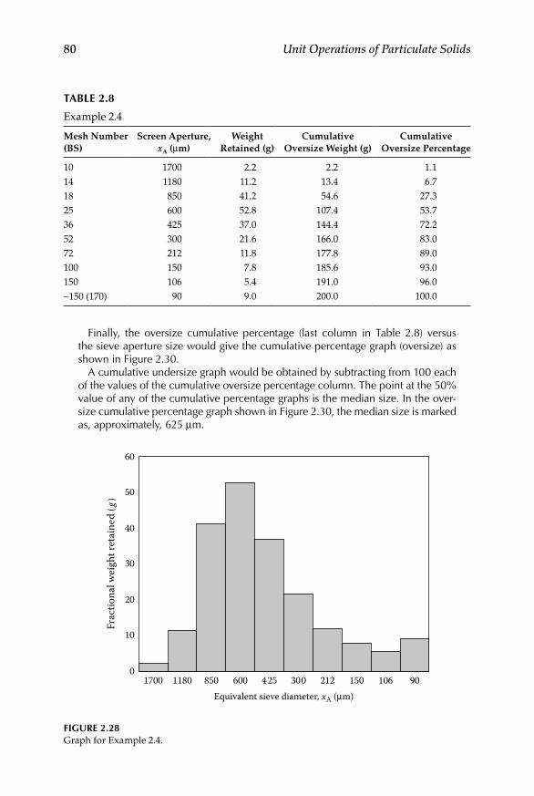
80 Unit Operations of Particulate Solids
Finally, the oversize cumulative percentage (last column in Table 2.8) versus the sieve aperture size would give the cumulative percentage graph (oversize) as shown in Figure 2.30.
A cumulative undersize graph would be obtained by subtracting from 100 each of the values of the cumulative oversize percentage column. The point at the 50% value of any of the cumulative percentage graphs is the median size. In the over-size cumulative percentage graph shown in Figure 2.30, the median size is marked as, approximately, 625 μm.
0
10
20
30
40
50
60
1700 1180 850 600 425 300 212 150 106 90Equivalent sieve diameter, xA (μm)
Frac
tiona
l wei
ght r
etai
ned
(g)
Figure 2.28Graph for Example 2.4.
Table 2.8
Example 2.4
Mesh Number (BS)
Screen Aperture, xA (μm)
Weight Retained (g)
Cumulative Oversize Weight (g)
Cumulative Oversize Percentage
10 1700 2.2 2.2 1.114 1180 11.2 13.4 6.718 850 41.2 54.6 27.325 600 52.8 107.4 53.736 425 37.0 144.4 72.252 300 21.6 166.0 83.072 212 11.8 177.8 89.0100 150 7.8 185.6 93.0150 106 5.4 191.0 96.0−150 (170) 90 9.0 200.0 100.0

Bulk Solids 81
2.6.6.3 Sedimentation
The methods based on sedimentation are probably the most numerous and varied of all particle sizing techniques. They measure the Stokes’ diameter of the particle and, therefore, measure the variable which is often most required to describe the behavior of the particles in suspension. There are some limi-tations with respect to particle shape in sedimentation analysis as particles that diverge grossly from spheres would not fall in a vertical pattern and, hence, the results when compared with other methods will tend to show
0
10
20
30
40
50
60
1700 1180 850 600 425 300 212 150 106 90Equivalent sieve diameter, xA (μm)
Frac
tiona
l wei
ght r
etai
ned
(g)
Figure 2.29Graph for Example 2.4.
0102030405060708090
100
200 400 600 800 1000 1200 1400 1600 18000
Cum
ulat
ive w
eigh
t per
cent
ove
rsiz
e
Equivalent sieve diameter, xA (μm)
Figure 2.30Graph for Example 2.4.
82 Unit Operations of Particulate Solids
oversize material. The two most common methods of particle size measure-ment by sedimentation are gravimetric and centrifugal sedimentation.
Gravity sedimentation is normally carried out by using the “Andreasen” pipette technique. In its simplest form, a suspension of approximately 0.1% by volume of particles is placed in a measuring cylinder, and a pipette used to withdraw 10 mL from a fixed depth below the surface. Such an apparatus is shown in Figure 2.31. The concentration of samples are measured and compared with the initial one. Since all the particles will settle at their termi-nal velocities, the ratio of the two concentrations is the fractional weight of particles to have reached a depth of H cm. Excluded will be the particles with a diameter smaller than xst (Table 1.2) as given in the relationship:
x
Hgtst
s= −
18µρ ρ( )
(2.36)
where μ is the liquid viscosity, ρs is the particle density, ρ is the liquid den-sity, g is the acceleration due to gravity, and t is the time.
From the fractional weight evaluated by Equation 2.36 the fraction under-size of a given powder can be determined. Allen (1981) has shown that varia-tions in concentration within a settling suspension can be related to cumulative percentage undersize F(x) by the equation
F x
C H tC H
( )( , )( , )
=0
(2.37)
where C(H, t) is the concentration in weight by volume at a depth H and time t, and C(H, 0) is the concentration in weight by volume at depth H and time zero. The timescale recommended for sample withdrawal (Allen, 1981) is the first sample at 1 min and then continuing in a geometric progression at a ratio equal to 2, that is, 2 min, 4 min, 8 min, and so on, as to obtain a smooth curve when plotting cumulative percentage undersize against Stokes’ diam-eter because of the inherent skewed distribution of most powders.
2.6.6.4 Centrifugation
Centrifugal sedimentation can be used to extend the range of applicability of sedimentation to the submicron size. Centrifugal sedimentation can be car-ried out using a pipette centrifuge that consists of a bowl centrifuge equipped with a withdrawal device connected to a pipette. The principle of particle size evaluation is similar to that used in the Andreasen Pipette, except that the particle is subjected to centrifugal acceleration, instead of gravity force, giving thus the possibility of detecting particles well below the submicron range at reasonably short periods of time. A diagram of the apparatus is

Bulk Solids 83
20
10
0
cm
Figure 2.31Andreasen’s sedimentation pipette.
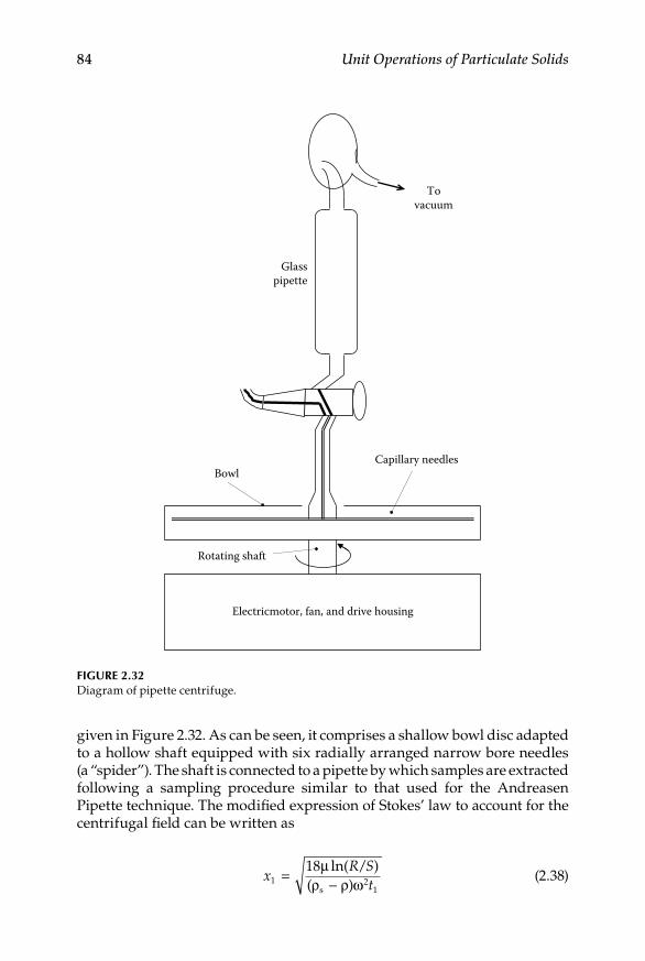
84 Unit Operations of Particulate Solids
given in Figure 2.32. As can be seen, it comprises a shallow bowl disc adapted to a hollow shaft equipped with six radially arranged narrow bore needles (a “spider”). The shaft is connected to a pipette by which samples are extracted following a sampling procedure similar to that used for the Andreasen Pipette technique. The modified expression of Stokes’ law to account for the centrifugal field can be written as
x
R St1 2
1
18= −
µρ ρ ω
ln( )( )
/s
(2.38)
Glasspipette
Tovacuum
Capillary needlesBowl
Rotating shaft
Electricmotor, fan, and drive housing
Figure 2.32Diagram of pipette centrifuge.
Bulk Solids 85
where x1 is the largest particle present in the initial sample with-drawn at time t1, when the measurement radius is R and the surface is at radius S, while ω is the angular velocity. Allen (1981) presents a procedure for particle size evaluation, analogous to that of the Andresen pipette, using Equation 2.33.
Gravity and centrifugal sedimentation can be combined for the same sample in order to directly determine Stokes’ diameter for a wide range of particle sizes. In such a way conversion are avoided and a mass distributions, appli-cable to processes where gravimetric efficiencies are relevant, can be properly derived. Ortega-Rivas and Svarovsky (1994) determined particle sizes distri-butions of fines powders using a combined Andreasen Pipette-pipette centri-fuge method. They derive relations useful to model hydrocyclone separations, which were later employed to describe apple juice clarification.
Another alternative to speed up a sedimentation particle size measure-ment is by using an instrument known as photosedimentometer. It operates by exposing the stream flow of a suspension containing the particles to be sized, through a cell across which a light beam is passed. As each particle passes through the beam it blocks a proportion of this according to the cross-sectioned arch of the particle. The number of particles in preset size levels is, thus, easily recorded. Instruments like the photosedimentometer, using a light-blocking technique will, however, have problems in measur-ing particles whose refractive indices are close to those of the carrier liq-uid. In general terms, they run into problems with particles smaller than 2 μm size.
2.6.6.5 Light Diffraction
Another way of taking advantage of light sources is the use of laser diffrac-tion as a means of detecting particles both in liquid or air streams. The basic principle on which these instruments work is shown in Figure 2.33. In essence, the presence of particles in a light beam causes light diffraction. This action results in a set of light rings at various radii to the incident beam. Each set of diffraction rings is spaced radially at a distance funda-mentally related to a specific particle diameter. The size range covered by instruments employing this principle is approximately 2–500 μm. They are ideally suited to process control operations where results are required quickly with a minimum operator attention. Recent developments in the use of laser diffraction techniques have enabled particles in the submicron range to be analyzed.
2.6.6.6 Particle Counters
In instrumental particle counters, such as the well-known Coulter coun-ter, the stream containing the particles is forced to pass through a flow

86 Unit Operations of Particulate Solids
restriction which is subjected to an electrical field. The normal flow of elec-trical current between the poles is altered by the particles passing through the restriction. These electrical flow changes, function of size of particle passing, are registered as pulses, then counted and grouped according to size. These sort of counters will count and size particles over a range from 800 μm down to 0.5 μm and, as the basic response is related directly to par-ticle volume, the instruments are for all practical purposes independent of problems associated with particle shape, color, or density, which affect most other methods.
2.6.6.7 Online Measurement Techniques
Automation of process control has created a need for continuous monitor-ing of particle size of particulate matter in process streams. Some online particle size analysis instrumentation has been developed recently to meet this need. It can initiate regulatory or shutdown signals in control systems. The basic requirements for such instrumentation are that it must operate automatically and continuously under preset instructions, and the response time from observations to readout must be so short as to be nearly instanta-neous. This relatively new range of techniques follows the general pattern found in the whole subject of particle size measurement. Some just give a measure of central tendency (mean diameter), others give one or more points on the size distribution. They may be truly online in operating on the whole process stream, they may need a partial sample stream taken off the main
Laser beamSmall
particle
Largeparticle
Ring detector
Figure 2.33Principle of operation of a laser diffraction particle counter.

Bulk Solids 87
one, or they may merely be automated rapid response batch techniques. Online measurement is a buoyant area that is undergoing fast growth. Equipment may be broadly divided into two categories: stream scanning and field scanning. Stream scanning would include different techniques following the basic principle described in the previous section adapted online to various processes. Field scanning usually applies to concentrated systems in which some size dependent behavior of the bulk material is monitored and particle size deduced from theoretical or calibrated relation-ships. Ultrasonic attenuation, echo measurements, laser attenuation, online viscometry, electric noise correlation techniques, x-ray attenuation, and x-ray fluorescence are examples of such field scanning methods. Most relevant to solid–liquid separation problems are those field scanning instruments which deduce particle size from separation efficiency of some separational equipment using the concept of the analytical cut size. Within these methods, wet sieving machines and separation performance hydrocyclones can be mentioned.
example 2.5
A sample of calcium carbonate is poured into water to make a test using an Andreasen Pipette. Dispersant is added at a concentration of 0.093% by weight. The density of the calcium carbonate is 2774 kg/m3. Fifteen samples are extracted starting at one minute and following a geometric progression at a 2 ratio. The initial height of the suspension in the Andreasen apparatus is 19.8 cm, and it is observed that every extraction decreases the level 0.4 cm. A container is weighed to determine the initial concentration of the powder in the suspension. Its initial weight (empty) is 1.31275 g, and after drying a 10 mL sample its final weight is 1.43655 (the sample contains the dispersant). Determine the powder median size using a cumulative percentage graph derived from data presented in Table 2.9.
SoluTion
Since extractions are done following a 2 progression ratio, the sampling times would be at 1 min, 2 min, 4 min, 8 min, and so on until reaching the 15th sample. On the other hand, the initial level in the Andreasen container is 19.8 cm, then in the second extraction it would drop to 19.4 cm, in the third extraction would drop to 19.0 cm, and so on, until reaching the last extraction. In each extraction the frac-tion of particles having a definite size, function of height, and time as expressed in Equation 2.36 can be related to the initial concentration including all the range of particle sizes, according to Equation 2.37. For example, the fraction of particles having the diameter corresponding to 19.8 height and 1 min time (sample 1), can be calculated by weight difference between the final weight of the container and the initial weight of the container (bearing in mind that the weight of dispersant, which form a solution with the suspending water, has to be subtracted from each sample). Since the dispersant has 0.093% by weight, there will be 0.0093 g of dispersant in each 10 mL sample. Thus, the weight fraction of the first extracted sample
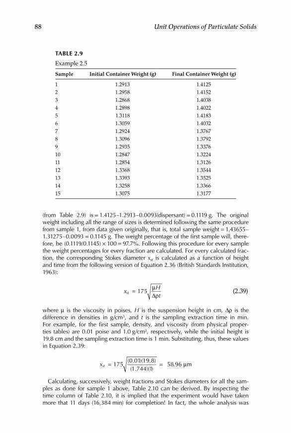
88 Unit Operations of Particulate Solids
(from Table 2.9) is = 1.4125–1.2913–0.0093(dispersant) = 0.1119 g. The original weight including all the range of sizes is determined following the same procedure from sample 1, from data given originally, that is, total sample weight = 1.43655–1.31275–0.0093 = 0.1145 g. The weight percentage of the first sample will, there-fore, be (0.1119/0.1145) × 100 = 97.7%. Following this procedure for every sample the weight percentages for every fraction are calculated. For every calculated frac-tion, the corresponding Stokes diameter xst is calculated as a function of height and time from the following version of Equation 2.36 (British Standards Institution, 1963):
x
Ht
st = 175µ
ρ∆ (2.39)
where μ is the viscosity in poises, H is the suspension height in cm, Δρ is the difference in densities in g/cm3, and t is the sampling extraction time in min. For example, for the first sample, density, and viscosity (from physical proper-ties tables) are 0.01 poise and 1.0 g/cm3, respectively, while the initial height is 19.8 cm and the sampling extraction time is 1 min. Substituting, thus, these values in Equation 2.39:
xst 58 96 m= =175
0 01 19 81 744 1
( . )( . )( . )( )
. µ
Calculating, successively, weight fractions and Stokes diameters for all the sam-ples as done for sample 1 above, Table 2.10 can be derived. By inspecting the time column of Table 2.10, it is implied that the experiment would have taken more that 11 days (16,384 min) for completion! In fact, the whole analysis was
Table 2.9
Example 2.5
Sample Initial Container Weight (g) Final Container Weight (g)
1 1.2913 1.41252 1.2958 1.41523 1.2868 1.40384 1.2898 1.40225 1.3118 1.41836 1.3059 1.40327 1.2924 1.37678 1.3096 1.37929 1.2935 1.337610 1.2847 1.322411 1.2854 1.312612 1.3368 1.354413 1.3393 1.352514 1.3258 1.336615 1.3075 1.3177
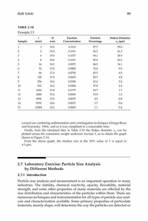
Bulk Solids 89
carried out combining sedimentation and centrifugation techniques (Ortega-Rivas and Svarovsky, 1994), and so it was completed in a reasonable time.
Finally, from the tabulated data in Table 2.10 the Stokes diameter xst can be plotted versus the cumulative weight undersize fraction F, as to obtain the graph shown in Figure 2.34.
From the above graph, the median size at the 50% value of F is equal to 4.5 μm.
2.7 Laboratory Exercise: Particle Size Analysis by Different Methods
2.7.1 introduction
Particle size analysis and measurement is an important operation in many industries. The stability, chemical reactivity, opacity, flowability, material strength, and some other properties of many materials are affected by the size distribution and characteristics of the particles within them. There are numerous techniques and instrumentation for all types of particle size anal-ysis and characterization available. Some primary properties of particulate materials, mainly shape, will determine the way the particles are detected or
Table 2.10
Example 2.5
Samplet
(min)H
(cm)Fraction
ConcentrationFraction
PercentageStokes Diameter
xst (μm)
1 1 19.8 0.1119 97.7 59.0
2 2 19.4 0.1101 96.2 41.3
3 4 19.0 0.1077 94.1 28.9
4 8 18.6 0.1031 90.0 20.2
5 16 18.2 0.0972 84.9 14.1
6 32 17.8 0.0880 76.8 9.9
7 64 17.4 0.0750 65.5 6.9
8 128 17.0 0.0603 52.7 4.8
9 256 16.6 0.0348 41.4 3.4
10 512 16.2 0.0284 37.8 2.4
11 1024 15.8 0.0179 24.7 1.7
12 2048 15.4 0.0083 10.8 1.2
13 4096 15.0 0.0039 4.9 0.8
14 8192 14.6 0.0015 1.7 0.6
15 16384 14.2 0.0009 1.1 0.4

90 Unit Operations of Particulate Solids
categorized by different particle size distribution measurement techniques. The objective of the exercise is to determine particle size distributions of industrial powders. At least two methods will be carried out with the same powder, in order to find out possible differences in the whole distribution as well as in the determination of the mean size.
2.7.2 Materials and instruments
A sample of medium-sized dolomite with particle sizes ranging from approx-imately 8–80 μm, and a second sample of coarse-sized dolomite having par-ticles in a range about 40–400 μm.
An optical microscope, a standard set of sieves, an Andreasen Pipette, and any versatile instrumental particle sizer, such as a laser diffraction equip-ment or an electrical sensing zone particle counter.
2.7.3 accessories
A hairline eyepiece, an ocular micrometer or standard graticule, and a stage micrometer, provided for microscopy. Routine laboratory material and ancil-lary instruments to carry out gravimetric testing, that is, balance, oven, des-iccator, measuring cylinders, stop watch, watch glasses, and so on.
0
10
20
30
40
50
60
70
80
90
100
0 10 20 30 40 50 60
Cum
ulat
ive w
eigh
t per
cent
und
ersiz
e
Equivalent stokes diameter, xst (μm)
Figure 2.34Graph for Example 2.5.

Bulk Solids 91
2.7.4 Microscopy Method
2.7.4.1 Introduction
Microscopic examination is one of the oldest, most direct, and simplest means for determining the size and size distribution of fine particles. Microscopic examination is tedious but gives reliable and reproducible results if careful measurements are made. As indicated in Table 2.6, micros-copy is applicable to particles sizes ranging from about 0.5 to 500 μm if an optical system is used.
2.7.4.2 Slide Preparation
Place a small sample of the powder onto a watch glass. Add a few drops of water containing a little teepol or other dispersing agent, except if the pow-der is water soluble, in which case an appropriate solvent should be used. Work the suspension with a small camel hair brush or glass rod. Add more or less liquid, so as to adjust the concentration of the suspension to give a representative selection of well-dispersed particles. Using the end of the brush or rod, transfer a drop of the suspension to a clean microscope slide. Cover with a slip taking care to avoid air bubbles.
2.7.4.3 Measurement of Particle Size
Once the particles are on the slide their diameters may be measured. However, since the particles are very likely to be irregular in shape, the meaning of “particle diameter” needs stating. Common equivalent diame-ters used in microscopy are the projected area diameter (Table 1.3) and statis-tical diameters, such as Feret’s or Martin’s diameters (Table 1.4). Feret’s and Martin’s diameter measurements must be taken in the same direction for all the particles. For the results to be statistically significant, measurements must be made on many particles. Counting of six particles in each of one hundred fields of view is often regarded as minimum.
2.7.4.4 Procedure
Using the stage micrometer, calibrate the eyepiece for a particular •object selected.
Make up the sample as outlined in Section 2.7.1.4. Use coarse-sized •dolomite.
Using the calibrated eyepiece measure a selected statistical diameter •(Feret’s or Martin’s diameter). Measure the diameters of 10 particles in, as many fields of view as possible, but not less than 10.

92 Unit Operations of Particulate Solids
Replace the calibrated hairline by the globe and circle graticule pro-•vided and with the stage micrometer, calibrate either the globe or the circles. Using the calibrated graticule measure the projected area diameter of 10 particles in, as many fields of view as possible, but not less than 10.
2.7.4.5 Calculations and Report
Tabulate range of size versus the number of particles counted within •the most convenient range of sizes selected.
Follow a procedure similar to that of Example 2.4, in order to elabo-•rate a histogram, a frequency curve, and an undersize cumulative percentage graph, and determine the median size of the powder (note that the particle size distribution obtained will be by num-ber, while in Example 2.4 the particle size distribution obtained was by mass).Perform a literature search to find out particle size distributions of •similar materials and compare type of graphs shown and median sizes reported.Present a complete written report, according to scientific report •guidelines, either given by instructor or consulted in the literature. Include graphs, charts, and calculations carried out.
2.7.5 Screening Method
2.7.5.1 Introduction
In a size analysis by screening, material is successively passed over a series of sieves having progressively smaller openings. Particles are passed or retained on a particular aperture size of sieve surface. The object of the experiment is to determine the size distribution of coarse-sized dolomite and compare the results with those of the microscopy counting method.
2.7.5.2 Choice of Sieves
Weight a sample of 200 g of powder to be tested. Take a sieve of the top range of openings and a sieve of the bottom range of opening. By visual judgment and trial and error, work out a pair or distant sieve opening so that not more than about 5% of the sample weight should pass the finest sieve or be retained on the coarsest, that is, 10 g passing through the finest sieve and 10 g retained on the coarsest sieve. Once the terminal sieves have been decided upon, the intermediate sieves can then be chosen. For most purposes the ratio of diam-eters of openings in two successive sieves is: 1: 2, for example, if the sieve range chosen is 16–60 mesh (BS Test Sieves Series), the choice to give a x series would be: 16, 22, 30, 44, 60.

Bulk Solids 93
2.7.5.3 Procedure
Weight a fresh sample of 200 g coarse-sized dolomite.•
Select the screens of the series determined by the procedure described •above in Section 2.7.5.2.
“Nest” the chosen sieves together with collection pan and lid.•
Place the weighed sample on the top sieve, assemble the nest on the •vibratory unit, and vibrate for about 5 min. carefully remove any fines from the pan at the bottom of the nest. Replace the pan and vibrate for another 2 min. Remove the pan again and take of any fines therein. Repeat the procedure until no more fines are collected in the pan.
Carefully disassemble the unit and weight the material left on each •sieve, making note of the sieve aperture size for each sieve.
2.7.5.4 Calculations and Report
Follow a procedure similar to that of Example 2.4, in order to elabo-•rate a histogram, a frequency curve, and an undersize cumulative percentage graph, and determine the median size of the powder.Compare the results with those from the exercise of the microscopy •method, and with results reported in the literature for similar mate-rial and same, or different, particle measurement techniques.Present a complete written report, according to scientific report •guidelines either given by instructor or consulted in the literature. Include graphs, charts, and calculations carried out. Discuss on the comparisons made above.
2.7.6 Sedimentation Method
2.7.6.1 Introduction
Different sizes of particle settle at different terminal velocities, and this property can be used in several ways to determine the size distribution of a sample. In the Andreasen Pipette a sample of the material is dispersed in a liquid and allowed to settle from time zero. At intervals a sample of fluid is extract from a depth H below the surface. These samples are evaporated to dryness and weighed to give concentrations. This produces a set of concen-trations Ct and the known initial concentration C0. At any time t the sample withdrawn will contain particles with terminal velocities equal to or less than H/t, at their original concentration, larger particles will have settled below the level of the pipette tip. The objective of the experiment is to determine the particle size distribution of dolomite powder, and compare
94 Unit Operations of Particulate Solids
the results obtained with an instrumental method of particle size measurement.
2.7.6.2 Preparation of Sample
Use the medium-sized dolomite sample to prepare a suspension of, approxi-mately, 0.5% by weight. Work out the weight of sample by using its density. For typical inert powders, 5–10 g in a liter of suspending medium will pro-duce a 0.5–2% by weight suspension. Use as suspending medium a 0.1%, by weight, aqueous solution (distilled water) of sodium hexametaphosphate as dispersant. Prepare a set of weighing containers for gravimetric determina-tion of sample concentration. Aluminum dishes, like those used for cup cakes, may be used for this purpose. It is advisable to prepare the dishes needed for each run by placing them in an oven at 100°C for about 2 h, and allow them to attain room temperature in a desiccator for another 2 h. The desiccator should contain only one layer of dishes. Weigh the dishes to 0.1 mg. Record their weights. Calculate gravimetrically the dispersant concentra-tion, as well as the initial sample concentration, using previously prepared and weighed aluminum dishes.
2.7.6.3 Procedure
Fill up the vessel of the Andreasen Pipette with the sample suspension. •Agitate thoroughly. Start the stop watch.Extract samples operating the two-way stopcock to fill the 10 mL •bulb by suctioning, and emptying the extracted sample by gravity or blowing on the corresponding weighed dish by turning to the sec-ond position of the stopcock.Continue sampling following a 2 progression ratio until the last pro-•grammed extraction.Take dishes with samples to an oven, in order to evaporate the sus-•pending medium until complete dryness.Allow the samples to cool down and attain room temperature in a •desiccator for, at least, 2 h.Weigh the dried and conditioned-to-room-temperature aluminum •dishes. Record the final container weights.
2.7.6.4 Calculations and Report
Follow the procedure described in solution of Example 2.5 to calcu-•late, successively, weight fractions and Stokes diameters for all the samples.Construct a table similar to Table 2.10, with the collected data of the •experiment.

Bulk Solids 95
From the tabulated data draw a graph of the Stokes diameter • xst ver-sus the cumulative weight undersize fraction F, as to obtain a plot like the one shown in Figure 2.34.From the graph obtained read the median size at the 50% value of • F.
2.7.7 instrumental Method
2.7.7.1 Introduction
Instrumental techniques for measurement of particle size distribution of powders have had a tremendous advancement in recent times. Numerous methods and procedures have been developed at a steady pace over the years, and there is the possibility of covering the wide spectrum from nanosystems, to ultrafine powders, and to coarse particulate assemblies. Many instruments offer nowadays quick, reliable results for a wide variety of powders and par-ticulate systems, and for a number of applications. There is still, however, the need to understand the basic principles under which sophisticated instru-ments operate, as well as to resource to direct measurements under some cir-cumstances. Some of the most modern instrumental techniques are based on an indirect measurement and carry out transformations among the different ways of expressing particles size distributions, that is, by number, surface, or mass. Sometimes it is advisable to avoid transformations because instru-ments assume a constant shape coefficient on such transformation, which is not necessarily the case, and overestimation or underestimations of size of certain particles may arise. Also, in very specific applications, or in cases of basic or applied research, is better to measure directly the most relevant par-ticle size and particle size distribution. For example, if research is carried out in modeling of solid–liquid separations, a direct measurement of the Stokes equivalent diameter would be most appropriate. The aim of the exercise is to measure the particle size distribution of a sample of medium-sized dolomite, and compare the results with those of the Andreasen Pipette method.
2.7.7.2 Procedure
Use any instrumental technique for measurement of particle size distribu-tion, to determine the particle size distribution of the medium-sized dolo-mite. Follow up the procedure described in the manual of the instrument.
2.7.7.3 Calculations and Report
Gather the information given by the instrument and compare graphs, median size, and any other details about the analysis provided by the instrument, with the corresponding values previously determined using the Andreasen Pipette method. Compare results, also, with data from a literature search and present a written report, including a thoughtful discussion on the compara-tive aspects mentioned.
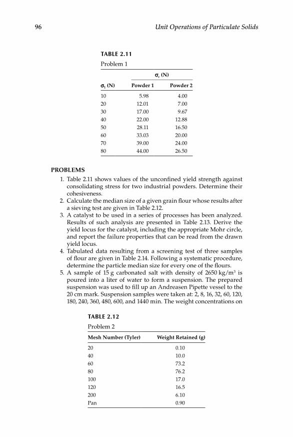
96 Unit Operations of Particulate Solids
PROBLEMS
1. Table 2.11 shows values of the unconfined yield strength against consolidating stress for two industrial powders. Determine their cohesiveness.
2. Calculate the median size of a given grain flour whose results after a sieving test are given in Table 2.12.
3. A catalyst to be used in a series of processes has been analyzed. Results of such analysis are presented in Table 2.13. Derive the yield locus for the catalyst, including the appropriate Mohr circle, and report the failure properties that can be read from the drawn yield locus.
4. Tabulated data resulting from a screening test of three samples of flour are given in Table 2.14. Following a systematic procedure, determine the particle median size for every one of the flours.
5. A sample of 15 g carbonated salt with density of 2650 kg/m3 is poured into a liter of water to form a suspension. The prepared suspension was used to fill up an Andreasen Pipette vessel to the 20 cm mark. Suspension samples were taken at: 2, 8, 16, 32, 60, 120, 180, 240, 360, 480, 600, and 1440 min. The weight concentrations on
Table 2.12
Problem 2
Mesh Number (Tyler) Weight Retained (g)
20 0.1040 10.060 73.280 76.2100 17.0120 16.5200 6.10Pan 0.90
Table 2.11
Problem 1
σc (N)
σ1 (N) Powder 1 Powder 2
10 5.98 4.0020 12.01 7.0030 17.00 9.6740 22.00 12.8850 28.11 16.5060 33.03 20.0070 39.00 24.0080 44.00 26.50

Bulk Solids 97
10 mL of the every extracted sample were: 0.1465, 0.0967, 0.0883, 0.0632, 0.0386, 0.0294, 0.0178, 0.0104, 0.0073, 0.0051, 0.0030, and 0.0008 g. If every extracted sample drops the height level in the vessel 0.5 cm, evaluate the median size of the carbonated salt particles.
References
Allen, T. 1981. Particle Size Measurement. London: Chapman & Hall.Allen, T. and Khan, A. A. 1970. Critical evaluation of powder sampling procedures.
Chemical Engineering 238: CE108–CE112.Augenstein, D. A. and Hogg, R. 1978. An experimental study of the flow of dry pow-
ders over inclined surfaces. Powder Technology 19: 205–215.Beddow, J. K. and Meloy, J. K. 1980. Testing and Characterization of Powders and Fine
Particles. London: Heyden and Son.Beke, B. 1964. Principles of Comminution. Budapest: Publishing House of the Hungarian
Academy of Science.
Table 2.13
Problem 3
Shear Stress (kPa) Normal Stress (kPa)
0.80 0.31.60 1.02.00 1.52.25 2.22.31 2.62.32 2.8
Table 2.14
Problem 4
Weight Retained (g)
Mesh Number (Tyler) A B C
20 6.00 0.10 0.4040 44.00 10.00 1.1060 29.00 73.20 2.0080 75.00 76.20 3.50
100 23.00 17.00 12.10120 2.00 16.50 61.80200 0.80 6.10 80.00PLT 0.20 0.90 39.10
98 Unit Operations of Particulate Solids
Bergstrom, B. H. 1966. Empirical modification of the Gaudin–Meloy equation. AIME Transactions 235: 45–45.
British Standards Institution. 1963. BS 3406: 1963. Part 2: Methods for the Determination of Particle Size of Powders—Liquid Sedimentation Methods. London: BSI.
British Standards Institution. 1970. BS 4140: 1970. Part 9: Determination of Angle of Repose. London: BSI.
Carr, R. L. 1965. Evaluating flow properties of solids. Chemical Engineering (January 1965): 163–168.
Carr, R. L. 1976. Powder and granule properties and mechanics. In Gas–Solids Handling in the Processing Industries, Marchello, J. M. and Gomezplata, A. (eds.). New York, NY: Marcel Dekker.
Carr, R. L. and Walker, D. M. 1968. Annular shear cell for granular materials. Powder Technology 1: 369–373.
Chasseray, P. 1994. Physical characteristics of grains and their byproducts. In Primary Cereal Processing, Godon, B. and Willm, C. (eds.). New York, NY: VCH Publishers.
Chen, X. D. 1994. Mathematical analysis of powder discharge through longitudinal slits in a slowly rotating drum: Objective measurements of powder flowability. Powder Technology 21: 421–437.
Dodge, H. F. and Romig, H. G. 1998. Sampling Inspection Tables. Single and Double Sampling. New York, NY: John Wiley and Sons.
Freeman, R. and Cooke, J. 2006. Testing powders in process relevant ways. Powder Handling & Processing 18: 84–87.
Freeman, R. E., Cooke, J. R., and Schneider, L. C. R. 2009. Measuring shear properties and normal stresses generated within a rotational shear cell for consolidated and non-consolidated powders. Powder Technology 190: 65–69.
Geldart, D. 1973. Types of gas fluidization. Powder Technology 7: 285–292.Geldart, D. and Wong, A. C. Y. 1985. Fluidization of powders showing degrees of
cohesiveness-II. Experiments on rates of de-aeration. Chemical Engineering Science 40: 653–661.
Geldart, D., Mallet, M. F., and Rolfe, N. 1990. Assessing the flowability of powders using angle of repose. Powder Handling and Processing 2: 341–345.
Gy, P. M. 1982. Sampling of Particulate Materials—Theory and Practice. Amsterdam: Elsevier.
Harris, C. C. 1968. The application of size distribution equations to multi-event comminution processes. AIME Transactions 241: 343–358.
Harris, C. C. 1971/1972. A multi-purpose Alyaudin–Rosin–Rammler–Weibull chart. Powder Technology 5: 39–42.
Herdan, G. 1960. Small Particle Statistics. London: Butterworths.Hong, G.-H. and Watanabe, K. 2000. Powder bed tester. An instrument for measuring
the powder yield locus. In: Processing. Part IV, Wöhlbier, R. H. (ed.). Clausthal-Zellerfeld, Germany: Trans Tech Publications.
Jenike, A. W. 1964. Storage and Flow of Solids. Bulletin No. 123 of the Utah Engineer Experiment Station. Salt Lake City, UT: University of Utah.
Kaye, B. H. 1981. Direct Characterization of Fine Particles. New York, NY: John Wiley and Sons.
Kennedy, J. and Neville, A. M. 1986. Basic Statistical Methods for Engineers and Scientists. New York, NY: Harper & Row.
Larson, H. J. 1995. Introduction to Probability. New York, NY: Addison-Wesley.

Bulk Solids 99
Masuda, H. 1997. Powder sampling. In Powder Technology Handbook, Gotoh, K., Masuda, H., and Higashitani, K. (eds.). New York, NY: Marcel Dekker.
Mutsers, S. M. P. and Rietema, K. 1977. The effect of interparticle forces on the expan-sion of a homogeneous gas-fluidized bed. Powder Technology 18: 239–242.
Ortega-Rivas, E. and Svarovsky, L. 1994. A direct combined method for measuring particle size distribution in obtaining grade efficiency curves. Powder Handling and Processing 6: 401–404.
Peleg, M. 1977. Flowability of food powders and methods for its evaluation—A review. Journal of Food Process Engineering 1: 303–328.
Peleg, M. and Normand, M. D. 1986. Simulation of size reduction and enlargement processes by a modified version of the beta distribution function. AIChE Journal 32: 1928–1930.
Peleg, M., Normand, M. D., and Rosenau, J. R. 1986. A distribution function for par-ticle populations having a finite size range and a mode independent of the spread. Powder Technology 46: 209–214.
Plowman, P. M. 1985. Practical aspects of sampling. Bulk Solids Handling 5: 1259–1265.Rietema, K. and Mutsers, S. M. P. 1973. The effect of interparticle forces on the expan-
sion of a homogeneous gas fluidized bed. Proceedings International Symposium of Fluidization and Its Applications. Tolouse, France.
Rietema, K., Boonstra, J., Schenk, G., and Verkooijen, A. H. M. 1980. The interaction between gas and dispersed solids and its effect on handling operation of solids. Proceedings of the European Symposium on Particle Technology. Amsterdam, the Netherlands.
Rittinger, P. R. 1867. Lehrbauch der Aufbereitungskunde. Berlin: Ernst and Korn.Schulze, D. 2007. Powders and Bulk Solids: Behavior, Characterization, Storage and Flow.
New York, NY: Springer.Sutton, H. M. 1976. Flow properties of powders and the role of surface character. In
Characterization of Powder Surfaces, Parfitt, G. D. and Sing, K. S. W. (eds.). New York, NY: Academic Press.
Svarovsky, L. 2000. Solid–Liquid Separation. Oxford: Butterworth-Heinemann.Teunou, E. and Fitzpatrick, J.J. 2000. Effect of storage time and consolidation of food
powder flowability. Journal of Food Engineering 43: 97–101.Wilkinson, H. N., Dufferll, C. H., Reed, A. R., and Bunting, J. 1983. Bulk Solids Physical
Property Guide. Ascot, UK: British Material Handling Board.Williams, T. C., Birks, A. H., and Bhattacharya, D. 1970/1971. The direct measurement
of the failure function of a cohesive powder. Powder Technology 4: 328–337.Yu, A. B. and Standish, N. 1990. A study of particle size distribution. Powder Technology
62: 101–118.


101
3Storage and Conveying of Bulk Solids
3.1 Introduction: Storage Alternatives
In the materials processing industries there are some particulate systems, such as gravel or ores, which may be stored outdoors in large piles or heaps unpro-tected from the weather. When taking to process, such materials may be removed by dragline or tractor shovel and delivered to a conveyor. Since many bulk materials are able to deteriorate with outside ambient conditions such as moisture, there is a need to provide for protection to these piled particulate systems. Several alternatives that have been used, like domes and cylindrical structures with conical tops, are normally known as silos. Some of these struc-tured forms of storage have been termed according to a particular application, such as corrugated-wall structures known as grain silos. The reclaiming sys-tems for these types of silos are similar to those used in outdoors storage, that is, draglines, scraper reclaimers, bucket wheel reclaimers, and so on.
There are, however, numerous examples in many materials processing industries where different types of solids are to be stored in confinement, with the intention of being directly connected to processing lines by any sort of conveying system. The vessels used for confined storage of particulate solids are generally known as bins or silos. Difficulties of flow in particulate systems, when needed to be recovered from confined storage, is a well-known operative problem and diverse industries such as mining, chemical, and food industry have invested considerable time and money over the years trying to overcome such situation. Systematic study of solids flow behavior in bins and silos to ensure proper discharge, has been intensive since the formal starting of Powder, or Particle, Technology as a discipline. The pio-neering studies of Andrew W. Jenike (Jenike, 1964), established the founda-tion of silo design and operation.
3.2 Outdoors Storage
Outdoor and structured storage systems are useful when huge amounts of materials need to be in inventory but direct connection to feed processing

102 Unit Operations of Particulate Solids
lines is somewhat difficult. For storage of thousands of tons of particulate materials, proper of some industries like the mining and metallurgy indus-try, this alternative seems to be the only feasible choice. Estimation of surface area for storage can be done by scaling-up from small samples of the particu-late material, using a property like its angle of repose. Space allowance can be done by estimating the volume of the pile through aerial or ground sur-veys and multiplying by the bulk density of the material. If, as previously pointed out, environment outdoors conditions may affect the integrity of the stored piles of materials, an alternative to protect them would be the use of storage domes (Mitman, 1991; South, 1991).
Material reclaiming and feeding to processing lines can be carried out by manual or mechanized handling. The obvious trend is to use mechanized handling whenever feasible and possible. Apart from substantial savings when using mechanized handling for material reclaiming, additional advan-tages like efficiency in utilization of storage space, reduction of material wastage, reduction of operator fatigue, and improving control and rotation of stock, can be mentioned. Mechanized reclaiming systems include dra-glines, scraper reclaimers, bucket wheel reclaimers, and so on. The technol-ogy of stockpile storage is a bit outside of the scope of this book, but the reader may refer to valuable literature on the subject (McLean, 1990; Roberts and Teo, 1990; Walker, 1990; Wohlbier, 1977).
3.3 Confined Storage
Open-yard or structured storage may be only a part of a bulk solids handling facility. Due to processing requirements, there is normally the need of having an intermediate storage system which may be directly connected to a processing line. In some other cases, the storage capacity would not involve large tonnages and, therefore, confined storage would be an obvious choice. Furthermore, considering finely divided solids that are subjected to erosion by wind or rain, piling cannot be taken as a feasible manner of storage and, therefore, all these particulate systems may be most properly kept in containers or vessels known also as silos, but alternatively termed as bins and hoppers. In this case, a silo is tall and rela-tively small in diameter, while a bin is usually not so tall and fairly wide. A hopper is a small bin with a sloping bottom, for temporary storage of solids prior to be fed into a particular process. Normally, the lower part of a silo in a shape of a cone or inverted pyramid is also called a hopper. Generally, all these containers are loaded from the top and discharged from the bottom. A major problem in bin design is related to proper and controllable discharge.

Storage and Conveying of Bulk Solids 103
3.3.1 general Considerations
The materials processing industries handle considerable amounts of pow-ders and particulate materials every year. Silos, bins, and hoppers used to store these materials vary in capacity from a few kilos to multiton-capacity vessels. Start-up delays and ongoing inefficiencies are common in solids pro-cessing plants. An important cause of these problems is the improper design of bulk solids handling equipment. A six-year study of 40 solids processing plants in the United States and Canada (Merrow, 1988) revealed that 80% of these plants experienced solids handling problems. The study also found that these plants were slow in smoothing operation, with an average start-up time for some plants averaging 18 months. Once start-up began, performance around 40–50% of design was commonly observed.
The common flow problems in hoppers and silos can be summarized as follows: (a) no flow, (b) segregation, (c) flooding, and (d) structural failure. Lack of discharge in the no-flow situation can be attributed to the forma-tion of a stable arch over the outlet, or a stable cavity called a “rathole” (Marinelli and Carson, 1992). With regard to segregation, many materials experience separation of fine and coarse particles (Carson et al., 1986) and such separation can seriously compromise the quality of the final product as well as the efficiency of the process. Flooding can be caused by the col-lapse of a rathole in a bin containing fine powder, resulting in uncontrol-lable flow of material, loss of product and clouds of dust (Royal and Carson, 1993), among other problems. Pertaining structural failure, each year over 1000 silos, bins and hoppers fail in North America alone. Most of these failures could have been prevented with proper and careful design, in which the loads imposed by the bulk solid being stored, had been well considered.
The design of bins, hoppers, and silos has never been given the attention it deserves. Approaches using properties such as angle of repose or angle of spatula in design considerations are ineffective, because the resulting val-ues bear no relation to the design parameters needed to ensure reliable flow, mainly because particulate solids tend to compact or consolidate when stored. The attempt of trying to model bulk solids as fluids also leads to a bottleneck, due to the fact that flowing bulk solids generate shear stresses and are able to maintain these stresses even when their flow rate is changed dramatically. It is also improper to consider bulk solids as having viscosity since almost all bulk solids exhibit flow properties that are flow-rate inde-pendent. The systematic approach for designing powder handling and pro-cessing plants started in the mid-1950s by the pioneering work of Andrew W. Jenike. His concept was to model bulk solids using the principles of con-tinuum mechanics. The resulting comprehensive theory (Jenike, 1964) describing the flow of bulk solids has been applied and perfected over the years, but is generally recognized worldwide as the only scientific guide to bulk solids flow.
104 Unit Operations of Particulate Solids
The procedures for the design of a bulk solids handling plant are well established and follow four basic steps: (a) determination of the strength and flow properties of the bulk solids for the worst likely flow conditions expected to occur in practice; (b) calculation of the bin, stockpile, feeder, or chute geometry to give the desired capacity to provide a flow pattern with accept-able characteristics, in order to ensure that discharge is reliable and predict-able; (c) estimation of the loadings on the bin and hopper walls and on the feeders and chutes under operating conditions; (d) design and detailing of the handling plant including the structure and equipment.
3.3.2 Types of Silos
As stated earlier, silo is recognized as the more generic term to refer to ves-sels for storage of particulate solids. A silo is a tall vessel with circular section and relatively small diameter ending in a slope bottom part, which is referred to as hopper. Since the early 1960s, mostly from the pioneering work of Jenike (1964), certain terms describing flow patterns started to become common in silo, bin and hopper design. The general theory pertaining to gravity flow of bulk solids has been documented through the years (Arnold et al., 1982; Roberts, 1988) and, from a standpoint of flow patterns there are basically three types of flow in symmetrical geometry: mass flow, funnel flow, and expanded flow.
In mass-flow bins (Figure 3.1a) the hopper is sufficiently steep and smooth to cause flow of all the solids in the bin without stagnant regions during discharge. The bulk solid is in motion at every point within the bin when-ever material is drawn from the outlet. The flow is uniform and the bulk density of the feed is practically independent of the head of solids in the bin. Mass flow guarantees complete discharge of the bin contents at predictable flow rates. When properly designed, a mass-flow bin can remix the bulk of the solid during discharge even if segregation is promoted during filling. Mass-flow bins are classified according to the hopper shape and associated flow pattern. The main types of hoppers are: conical, wedge or chisel-shaped hoppers. Only conical hoppers operate with axisymmetrical flow, the remain-ing types tend to present a plane-flow pattern. In plane-flow bin, the slope to the vertical of the hopper is, on average, 8–10° larger than the corresponding value for axisymmetrical bins with conical hoppers. Therefore, they offer larger storage capacity for the same head room than the axisymmetrical bin, but this advantage may somewhat be offset by the long slotted opening needed, which can cause feeding problems. Figure 3.2 shows some hopper geometries indicating the type of flow. Mass-flow bins are generally recom-mended for cohesive materials, for materials which degrade with time, for fine powders, and for particulate systems which need to be prevented from segregation.
Funnel flow occurs when the hopper is not sufficiently steep and smooth to force the bulk solid to slide along the walls (Figure 3.1b). It is also

Storage and Conveying of Bulk Solids 105
observed when the outlet of the bin is not fully effective, due to poor feeder or gate design. In a funnel-flow bin the stored material flows toward the outlet through a vertical channel forming within stagnant solids. The diameter of such channel approximates the largest dimension of the effec-tive outlet. Flow out of this type of bin is generally erratic and gives rise to segregation problems. However, flow will continue until the level of the bulk solids in the bin drops an amount equal to the draw-down. At this level the bulk strength of the contained material is sufficient to sustain a stable rathole as illustrated in Figure 3.1b. Once the level defined by HD in this figure is reached, there is no further flow and the material below this level represents dead storage. For complete discharge the bin opening needs to be at least equal to the critical rathole dimension, determined at the bottom of the bin corresponding to the bulk strength at this level. For many cohesive bulk solids, and for the normal consolidation heads
Hcr
θ
B
θ
B
D(a) (b)
H
H
HD
Deadcapacity
D
Figure 3.1Types of flow patterns in hoppers. (a) Mass-flow. (b) Funnel-flow. D: silo diameter, H: average depth of material in cylindrical part, Hcr: critical depth to initiate flow in mass flow, HD: dynamic flow depth in funnel flow, θ: hopper slope, B: bottom aperture dimension.

106 Unit Operations of Particulate Solids
occurring in practice, ratholes measuring several meters high are often observed. This makes control of the product discharge rate quite difficult and funnel flow somewhat impractical. Funnel flow has the advantage of providing wear protection of the bin walls as the material flows against stationary material. However, it is a “first-in last-out” flow pattern which is unsatisfactory for fine bulk solids of low permeability. Such materials can aerate during discharge through the flow channel and this can give rise to flooding problems or uncontrolled discharge. Also, funnel-flow bins are
θ
B
B (D)
(a)
(c)
(b)
θθ
B
Figure 3.2Common hopper geometries. (a) Axisymmetrical flow, (b) symmetrical plane flow, and (c) nonsymmetrical plane flow.

Storage and Conveying of Bulk Solids 107
more prone to cause arching of cohesive solids than mass-flow bins and so they usually require larger outlets for dependable flow. Furthermore, this type of bin may cause segregation of solids and are unsuitable for solids that degrade with time in the stagnant regions. Cleanout of a funnel-flow bin is often uncertain because solid in the stagnant region may pack and cake. For all these reasons, funnel-flow bins are only suitable for coarse, free-flowing, or slightly cohesive, nondegrading solids when segregation is unimportant.
In expanded flow bins the hopper combines characteristics of mass flow and funnel flow, as illustrated in Figure 3.3. The higher part of the hopper operates in funnel flow while the lower operates in mass flow. The mass-flow outlet usually requires a smaller feeder than would be the case for funnel flow. The mass-flow hopper should expand the flow channel to a diagonal or diameter equal to or greater than the critical rathole diameter, thus eliminating the likelihood of ratholing. Funnel-flow bins provide the wall protection of funnel flow, along with the reliable discharge of mass flow. Expanded flow is ideal where large tonnages of bulk solids need to be stored and is particularly suitable for storing large quantities of bulk solids while maintaining acceptable head heights. The concept of expanded flow may be used to advantage in the case of bins or bunkers with multiple out-lets. Expanded flow bins are recommended for the storage of large quanti-ties of nondegrading solids. This design is also useful as a modification of
D
β
θ
B
Funnel-flow
Mass-flow
Figure 3.3Expanded-flow hopper.

108 Unit Operations of Particulate Solids
existing funnel-flow bins to correct erratic flow caused by arching, ratholing, or flushing.
3.3.3 Wall Stresses in axisymmetrical bins
The prediction of wall loads in bins is an important piece of information for their design. It is necessary to estimate the pressures at the wall which are generated when the bin is operated, in order to design the bin structure efficiently and economically. The approaches to the study of bin wall loads are varied and involve analytical and numerical techniques, such as finite-element analysis. Despite these varied approaches, it is clear that the loads are directly related to the flow pattern developed in the bin. The flow pattern in mass-flow bins is reasonably easy to predict but in funnel-flow bins such prediction becomes quite a difficult task. For this reason, unless there are compelling causes to do otherwise, bin shapes should be kept simple and symmetric.
Research relating to wall stresses dates back to the 1800s when Janssen (1895) published his now famous theory. More recent investigations (Walker, 1966; Jenike and Johanson, 1968, 1969; Walters, 1973; Clague, 1973) have shown that the solution of the problem of stress distributions in bins is extremely complex. However, most researchers agree that the loads acting on a bin wall are different during the initial stage of filling and during the stage of flowing in discharge, as represented in Figure 3.4. When bulk solids are charged into an empty bin, with the gate closed or the feeder at rest, the bulk solids settle as the solids head rises. In this settlement, the solids contract vertically in the cylindrical section and partially vertically in the hopper section. The major principal stress tends to align with the direction of contraction of the solids, forming which is termed as an active or peaked stress field. It is assumed that the solids are charged into the bin without significant impact to cause packing, and powders are charged at sufficiently low rate so that they deaer-ate. It is also assumed that the bin and feeder have been designed correctly for the solids to flow without obstruction. When the gate is fully opened or the feeder operates so that the solids start flowing out of the outlet, there is vertical expansion of the solids within the forming flow channel and the flowing mass of solids contract laterally. The major principal stresses within the flow channel tend to align with the lateral contractions and the stress field is said to be passive or arched.
The region of switch from active to passive stress field originates at the outlet of the bin, when the gate is opened or the feeder started, and rapidly moves upward into the bin as the solids are withdrawn. At the switch level a fairly large overpressure may be present, and it is assumed to travel upward with the switch at least to the level at which the channel intersects the verti-cal section of the bin. For a typical bin consisting of a hopper plus a cylindri-cal section above it, five stress fields have been recognized during the fill and discharge sequences: (a) in the cylindrical section during initial filling, where

Storage and Conveying of Bulk Solids 109
the state of stress is peaked or active; (b) in the cylindrical section during emptying, where the state of stress is either peaked or changes to arched, depending on whether the switch level is assumed to be caught at the transi-tion; (c) in the converging hopper section during filling, where the state of stress is assumed to be peaked; (d) in the converging hopper section during emptying, where the state of stress is assumed to be arched; (e) the switch field, the region in the bin where the peaked stress field established during initial filling is transformed into the arched stress field. This switch starts at the outlet of the hopper, if newly filled from completely empty, and then travels up very quickly as emptying continues, generally to become caught in the transition. Most of the researchers mentioned agree upon a wall pres-sure or stress distribution as shown in Figure 3.5.
The previously mentioned Janssen theory (Janssen, 1895) includes, possi-bly, the oldest reported attempt to calculate pressures in silos. Janssen derived an equation for the calculation of vertical and horizontal pressures and wall shear stresses. He assumed a vertical force balance at a slice element span-ning the full cross section of a silo being filled with bulk solids, and deter-mined the wall friction coefficient with a shear tester as well as the horizontal pressure ratio from pressure measurements in a model bin. He also assumed
Filling Emptying
Activeor
peakedstressfield
Passive orarched field
Figure 3.4Stress distribution in silos.

110 Unit Operations of Particulate Solids
a constant vertical pressure across the cross section of the slice element and restricted his evaluation to vertical silo walls. The Janssen equation for the vertical pressure pv on dependence of the depth h below the bulk solids top level reads as follows for a cylindrical silo:
p
g DK
K hD
vb e= −
−
ρ µ
41
4
µ′ ′
′ ′
(3.1)
where g is the acceleration due to gravity, ρb is the bulk density of solids, D is the silo diameter, μ’ is the sliding friction coefficient along the wall, and K’ is the ratio of the horizontal to the vertical pressure, which can be expressed as
K′ =
−+
11
sinsin
δδ
(3.1b)
where δ is the angle of internal friction of solids.The advantage of Janssen equation is the simplicity of an analytical equa-
tion and its general good agreement with pressure measurements in silos for
Mass-flow bin Static or fillcondition
Dynamic ordischarge condition
Normal wall load
Hei
ght
Hei
ght
Nor
mal
wal
l loa
d
Figure 3.5Wall load distribution in silo.
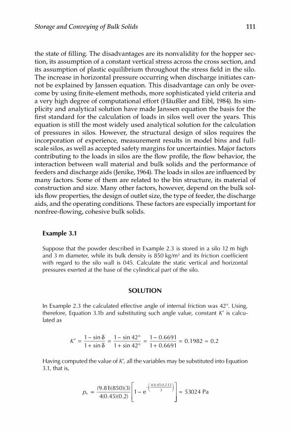
Storage and Conveying of Bulk Solids 111
the state of filling. The disadvantages are its nonvalidity for the hopper sec-tion, its assumption of a constant vertical stress across the cross section, and its assumption of plastic equilibrium throughout the stress field in the silo. The increase in horizontal pressure occurring when discharge initiates can-not be explained by Janssen equation. This disadvantage can only be over-come by using finite-element methods, more sophisticated yield criteria and a very high degree of computational effort (Häußler and Eibl, 1984). Its sim-plicity and analytical solution have made Janssen equation the basis for the first standard for the calculation of loads in silos well over the years. This equation is still the most widely used analytical solution for the calculation of pressures in silos. However, the structural design of silos requires the incorporation of experience, measurement results in model bins and full-scale silos, as well as accepted safety margins for uncertainties. Major factors contributing to the loads in silos are the flow profile, the flow behavior, the interaction between wall material and bulk solids and the performance of feeders and discharge aids (Jenike, 1964). The loads in silos are influenced by many factors. Some of them are related to the bin structure, its material of construction and size. Many other factors, however, depend on the bulk sol-ids flow properties, the design of outlet size, the type of feeder, the discharge aids, and the operating conditions. These factors are especially important for nonfree-flowing, cohesive bulk solids.
example 3.1
Suppose that the powder described in Example 2.3 is stored in a silo 12 m high and 3 m diameter, while its bulk density is 850 kg/m3 and its friction coefficient with regard to the silo wall is 045. Calculate the static vertical and horizontal pressures exerted at the base of the cylindrical part of the silo.
SoluTion
In Example 2.3 the calculated effective angle of internal friction was 42°. Using, therefore, Equation 3.1b and substituting such angle value, constant K’ is calcu-lated as
K′ δ °
°= −
+= −
+= −
+= ≈1
11 421 42
1 0 66911 0 6691
0 1982 0sinsin
sinsinδ
.
.. ..2
Having computed the value of K’, all the variables may be substituted into Equation 3.1, that is,
pv e= −
− ⋅ ⋅ ⋅
( . )( )( )
( . )( . )
. .9 81 850 34 0 45 0 2
14 0 45 0 2 12
3
≈ 53 24 Pa0

112 Unit Operations of Particulate Solids
Since K’ was defined as the ratio of the horizontal to the vertical pressure: ph = K’(pv), so that the horizontal pressure ph is
p K ph v a 1 6 5 Pa= = ≈( )( ) ( . )( )′ 0 2 53024 0 0P
The results are, thus vertical static pressure pv ~ 53 kPa, horizontal static pressure ph ~ 10.6 kPa.
3.3.4 Wall Stresses in other Types of Vessels
For the case of nonsymmetrical flow and some other complex flows like those presented in specific cases such as multioutlet silos, estimation of wall stresses is extremely difficult due to the absence of proximity of constant pressure on the vessels walls. Approaches for calculation in these types of vessels include modeling of a finite element for the interaction silo-solids (Mahmound, 1977) and a simplified theory consisting on describing flow of relatively small channels within a silo (Colijn and Peschl, 1981).
Adapting of silos has also been suggested to try to control pressures on the bins walls. A device for this purpose is known as the antidynamic discharge tube, used to minimize flow problems in tall grain silos. In this type of silo mass flow of grain occurs together with flow along the walls over a substan-tial height of the silo. This flow effect causes dynamic pressure generation of considerable higher magnitude (two- to threefold), than the static pressure developed in the silo after loading. It has been demonstrated (Thomson, 1997) that by using an antidynamic discharge tube is possible to control the flow pattern, so that funnel flow occurs without flow along the walls. The tube is located over the silo opening aligned to the geometric center and extended nearly all along the silo height. It contains perforations on its entire length to allow grain to enter the tube at different depth levels. On discharge the material flows through these orifices so that the solid only flows inside the tube, and over its top part, as shown in the diagram of Figure 3.6. Due to this flow pattern, the pressure exerted on the walls never exceeds the values of static pressure. A variation of the antidynamic discharge tube consists on a tube without perforations, place at a depth just below the half of the total silo height (Roberts, 1988b). Satisfactory results have been reported in silos with eccentric flow with multioutlet silos. Discharge tubes are only suitable for noncohesive, free-flowing solids such as grains and coarse sand. They should never be used with, even slightly, cohesive solids.
3.3.5 natural Discharge from Silos
Only fluids can flow; bulk solids under gravity forces can fall, slide or roll, but against gravity, they must be lifted by mechanical means. Solids cannot be pumped by centrifugal or reciprocating pumps; for pumping, bulk solids ought to be suspended in liquids or gases. There is no satisfactory term to

Storage and Conveying of Bulk Solids 113
describe “flow” of bulk solids as they do not follow strict definitions of fluid behavior, since a fluid is considered to be a continuum in which there are no voids. For a fluid, when the rate of shear is linearly proportional to the shear stress, it is said to be Newtonian and the coefficient of proportionality is called the absolute viscosity. Any deviation from this definition makes the fluid non-Newtonian. Solids in suspension can be referred to as non-Newto-nian mixtures to differentiate them from a number of non-Newtonian fluids which are a continuum or are perfectly homogeneous liquids. For all these reasons, bulk solids in suspension are occasionally referred to as “imperfect fluids.”
3.3.5.1 Flow Theories
The gravity flow of bulk solids occurs under the pressure corresponding to the equivalent of a “static head” of the material. Such head would be caused by the height of a solid column in a bin, but in practice is often not available to produce the flow due to phenomena known as “arching” or “bridging.” The velocity head at the discharge from the bin is usually a small fraction of the head, with the major part being consumed by the friction of the moving solids against the walls of the bin, as well as against like solids. Friction is the resistance which one body offers to the motion of a second body when the latter slides over the former. The friction force is tangent to the surfaces of
Figure 3.6Principle of antidynamic discharge tube.

114 Unit Operations of Particulate Solids
contact of the two bodies and always opposes motion. The coefficient of static friction for any two surfaces is the ratio of the limiting friction to the corre-sponding normal pressure. If a body rests on an inclined plane and if the angle of inclination of the plane to the horizontal is such that motion of the body impends, such angle is defined as the angle of repose. When two sur-faces move relative to each other, the ratio of the friction developed to the normal pressure is called the coefficient of kinetic friction and is indepen-dent of the normal pressure. The coefficient of kinetic friction is also less than the coefficient of static friction and independent of the relative velocity of the rubbing surfaces. There is experimental evidence suggesting that the value of the kinetic friction coefficient increases as the velocity is decreased, and passes without discontinuity into that of static friction. All these princi-ples would hold under conditions of a particular test, but must be modified in order to apply them to different conditions. It is, therefore, quite difficult to apply existing test data on a series of new tests because of the great variety of flowing conditions of bulk solids. The problem is particularly complicated since the properties of the flowing material depend on time and method of storage operation.
When granular solids are stored in an enclosed container, the lateral pres-sure exerted on the walls at any point is less than predicted from the head of the material above such point. There is usually friction between the wall and the solid particles, and the interlocking of these particles causes a frictional effect throughout the bulk solid mass. The frictional force at the wall tends to offset the weight of the solid and reduces the effect of the head of solids on the floor of the container. In an extreme case, such frictional force causes the mass of bulk solids to arch, or bridge, so that it would not fall even if the material below is discharged. For many granular solids, when the height of the solid bed reaches about three times the diameter of the bin, additional head of material shows virtually no effect on the pressure at the bin floor.
Solids tend to flow out of any opening near the bottom of a bin but are best discharged through an opening in the floor. The pressure at a side outlet is smaller than the vertical pressure at the same level and removal of solids from one side of a bin considerably increases the lateral pressure on the opposite side while the solids flow. When an outlet in the bottom of a bin containing free-flowing solids is opened, the material immediately above such opening begins to flow. A central column of solids moves downward without disturbing the material at the sides. Eventually lateral flow begins, starting from the top layer of solids and a conical depression forms in the surface of the mass of bulk solids being discharged. The material slides later-ally into the central column moving at an angle approaching the angle of internal friction of the solids and the solids at the bin floor are the last to leave. If additional material is added at the top of the bin, at the same rate as the material leaving through the bottom outlet, the solids near the bin walls remain stagnant and do not discharge as long as flow persists. The rate of flow of granular solids by gravity through a circular opening in the bottom

Storage and Conveying of Bulk Solids 115
of a bin is dependent on the diameter of the opening as well as on the proper-ties of the solid and is independent, within wide limits, on the head or height of the solids.
The amount of solids discharged through an opening in the bottom of a bin, and the failure to restart the flow after intermission, depend on the bin design, shape, and the location of the opening, apart from the flowing prop-erties of the solid. The flowing properties of the granular material include grain nature, size, moisture content, temperature, adhesion, cohesion, and, above all, time of consolidation at rest. There are very few solids that are free flowing and will restart flow after an extended period at rest. Examples of them include inert materials such as graded gravel and dry sand. Pressure distribution within a bin affects its design for strength, but does not enter into calculation of the solids flow from the hopper. It has been mentioned that the volume of bulk solids discharged is independent of the head above the orifice, due to the arching effect. Therefore, the design of bins or silos in terms of their ability to initiate flow without any aid, is based on solid mechanics theories considering only the hopper of the container.
The mass-flow and funnel-flow limits in silos are well known and have been used extensively in proper design. The limits for conical hoppers and plane hoppers depend on the hopper half-angle θ, the effective angle of inter-nal friction δ and the wall friction angle ϕ. Once the wall friction angle and effective angle of internal friction have been determined by experimental means, the hopper half angle θ may be determined. In function form it can be expressed as
θ ϕ δ= f ( , ) (3.2)
The bounds for conical and plane-flow hoppers are plotted for three values of δ in Figure 3.7. For the case of conical hoppers, it is recommended that the half-angle θ be chosen to be 3° less than the limiting value. For plane hoppers the bounds between mass-flow and funnel-flow are much less critical than for conical hoppers. In plane hoppers much larger hopper half-angles are possible, which means that the discharging bulk solids will undergo a significant change in direction as it moves from the cylindrical part to the hopper bottom.
Typically, flow in a hopper is based on the radial stress field theory, which does not take into account the influence of the surcharge head due to the cyl-inder on the flow pattern developed. It is, however, known that complete mass flow in a hopper is affected by the cylinder surcharge head. There is a mini-mum level Hcr (Figure 3.1), which is required to enforce mass flow in the hop-per. For a common mass-flow bin this level is from about 0.75D to 1.0D. Benink (1989) identified a third flow region, apart from mass flow and funnel flow, which has been known as intermediate flow. The three flow regions sug-gested by this author are illustrated in Figure 3.8. According to Benink (1989) the surcharge head has a significant influence on the flow pattern generated.

116 Unit Operations of Particulate Solids
In the study, fundamental relationships for Hcr in terms of the different bulk solids and hopper geometrical features are derived. These relationships are used to predict the critical height Hcr at which the flow changes.
3.3.5.2 Hopper Opening for Coarse Bulk Solids
Coarse bulk solids are those in which the particle size range is such that the air permeability is sufficiently high to allow air to percolate easily through
60
50Plane hopper
Funnel-flow
Mass-flow
δ = 60°δ = 50°δ = 40°
Conical hopperδ = 60°δ = 50°δ = 40°
40
30
20
10
10 20 30 40
Hopper half angle, θ (°)
Ang
le o
f wal
l fric
tion,
ϕ (°
)
50 60 70
Figure 3.7Limits for mass-flow in conical and plane-flow channels.
Mass-flow Funnel-flowIntermediateflow
Jenike’s limit(depends on δ)
Hopper half angle (θ)
Ang
le o
f wal
l fric
tion
(ϕ)
Limit dependson H/D and δ
Figure 3.8Flow regimes for plane-flow hopper defined by Benink (1989).

Storage and Conveying of Bulk Solids 117
the stored solids. According to the diagram shown in Figure 3.9, the acceler-ated flow of bulk solids in the region of the outlet of the hopper can be considered when the air pressure gradient Δpr equals zero. Analyzing the forces it may be shown that
σ
ρθ1 1= −
b gBH
ag( )
(3.3)
where σ1 is the stress acting in arch at angle 45°, ρb is the bulk density of solids, g is the acceleration due to gravity, B is the hopper opening, a is the acceleration of discharging bulk solids and H(θ) is a factor to account for variation in arch thickness, hopper half-angle, and hopper type, whether conical or plane. It has an approximate value of 2.2 for plane-flow hoppers and 2.4 for conical hoppers.
The minimum hopper opening to just prevent a cohesive arch from form-ing occurs when static equilibrium prevails, that is, when the acceleration of discharging bulk solids approaches zero, and thus, substituting a = 0 into Equation 3.3 and transposing:
B
Hgmin( )= σ θ
ρ1
b (3.4)
The hopper half-angle is chosen from the mass-flow limits as shown in Figure 3.7, while the condition for σ σ1 = c is obtained from the intersection
V0
Vav
Vs
ΔV
θT
σ1
B
ρg ΔV [1 – (a/g)]
ΔPr
Figure 3.9Flow channel and equilibrium of forces on the arch formed on a hopper.

118 Unit Operations of Particulate Solids
point of the flow factor ff line and failure function FF as illustrated in Figure 3.10. As discussed in the previous chapter, the failure function is a bulk solid parameter and represents bulk strength, while the flow factor is a flow channel parameter. The flow factor ff can be defined by the relationship:
ff 1
c= σ
σ (3.5)
The flow factor ff and function H(θ) are given as design curves (Jenike, 1964; Arnold et al., 1982; Roberts, 1988) like the one given in Figure 3.11. Following the work of Johanson (1965), it may be shown that the acceleration in Equation 3.4 may be expressed as
a g= −
1ffffa
(3.6)
where ff is the critical flow factor based on the minimum arching dimension and ffa is the actual flow factor based on the actual opening dimension. This actual flow factor may be represented as the relationship between stresses, according to Figure 3.10, by
ff =a
1
c
σσ
(3.7)
where σ1 is the major consolidation pressure at outlet corresponding to dimension B.
σ1
σ1 = σc
σc
FF
ffFlow No flow ffa
Figure 3.10Design graphic for hopper geometry.

Storage and Conveying of Bulk Solids 119
The acceleration has two components, that is,
a a a= +c v (3.8)
where ac is the convergence component due to flow channel and av is the component due to velocity increase as flow is initiated. This last component may be represented as a function by
a g
V mBv
a
ffff
= −
− +1
2 12( ) tan θ
(3.9)
where V is the discharge velocity and m is a constant which takes the value of zero for plane-flow hoppers and unity for axisymmetrical or conical hoppers.
Equation 3.9 shows that as the discharge velocity V increases, the compo-nent due to velocity increase as flow is initiated av tends to zero. Thus, an average terminal discharge velocity Va is reached when av = 0, that is,
V
Bgma
a= + −
2 1
1( )tan θ
ffff
(3.10)
The flow rate Q0 may be calculated by the following equation:
Q B L Vm m m0
1 1 4= + −ρ πb( ) ( ) ( / ) a (3.11)
40
30
20
10
ff = 1.4
1.5
1.6
1.8
10 20 30 40 50Hopper half angle (θ)
Ang
le o
f wal
l fric
tion
(ϕ)
23
4
Figure 3.11Flow factor graph for conical hopper and effective angle of internal friction, δ = 40°.

120 Unit Operations of Particulate Solids
where L is the length of slot for rectangular opening in plane-flow hoppers, in which case, B would represent the wide of slot. It can be easily seen that, for conical hoppers B would represent the diameter of the circular opening and, thus, Equation 3.10 above is applicable for both cases of plane-flow hoppers, either with square or slot opening, and axisymmetrical or conical hoppers.
For design purposes B and Q0 can be plotted as a function of θ, as presented in Figure 3.12. In such a way, several options of hopper geometry can be explored. In many cases the flow rate determined above the unim-peded discharge will be well in excess of the plant requirements. For this reason feeders may be used to control discharge rate to any required value.
3.3.5.3 Hopper Opening for Fine Bulk Solids
For the case of fine powders, discharge from a hopper will be rather diffi-cult due to the low permeability of the powder to the air flow. Flow rates much lower than those calculated by the method described above can be common in practice. The analysis of the flow process is much more com-plex and involves two-phase flow theory. The flow of fine powders has been studied over the years by several researchers such as McLean (1979), Arnold et al. (1982), and Arnold and Gu (1990). Larger hopper openings are required than for the equivalent coarse bulk solids and, sometimes, air permeation is needed to bias the pore pressure in the hopper in order to assist the discharge. Fine powders are prone to flooding and uncontrollable discharge, when allowed to aerate. For this reason extreme care should be taken in designing and installing any air permeation system. Care must also be exercised in ensuring that the interface between the hopper and feeder is correctly designed to prevent problems due to flooding.
000 B
Q0θ
Figure 3.12Hopper half-angle θ and mass flow rate versus hopper opening B.

Storage and Conveying of Bulk Solids 121
example 3.2
The powder characterized in Example 2.3 has the failure function given in Table 3.1 while its bulk density is 960 kg/m3. If the determined angle of wall friction is 18°, calculate the hopper opening and the discharge flow rate, considering that the term ff/ffa can be considered negligible.
SoluTion
The effective angle of internal friction determined in Example 2.3 was 42°, and so the design graph for 40° may be used for calculations. In such graph, the value of ϕ = 18 is prolonged until a distance 3° short from the limit line of funnel flow to read a value of ff = 1.5 (Figure 3.13). The inverse of ff will give the slope of the line to be drawn in the failure function graph, derived from Table 3.1. The slope of the line at a value of ff = 1.5 is 34°. Drawing a line of such slope in the graph of the failure function a value for σ1 would, therefore, be about 1180 N/m2 as indicated in Figure 3.14.
Substituting, thus, values in Equation 3.4:
B
Hg
min( ) ( )( . )
( )( . ). ~= = =σ θ
ρ1 1180 2 4
960 9 810 00 0
b
3 7 m 3 cm
To evaluate the discharge mass flow rate Q, the discharge velocity Va needs to be determined. The hopper half-angle is read of from Figure 3.13 as 28°, so that tan (28°) = 0.5317. For conical hoppers m = 1, and ff/ffa approaches zero. With all these figures and considerations, substituting into Equation 3.10:
VBg
ma
a
ffff
=+
−
=+
−[2 1
10 3 9 81
21 1 0 53171 0
( ) tan( . )( . )
( )( . )θ ]] = =2 9431 8652
..
.1176 m/s
Table 3.1
Example 3.2
σ1 (kPa) σc (kPa)
0.2 0.300.4 0.510.6 0.660.8 0.811.0 0.921.2 1.031.4 1.101.6 1.161.8 1.182.0 1.20

122 Unit Operations of Particulate Solids
Equation 3.11 for a value of m = 1 would reduce to the expression below. Substituting the derived value Va above and the hopper opening dimension calculated previously:
Q
BV0
2 2
4960
0 34
1 176=
=
=ρ π πb a 79 82 kg/s
( )( )
( . )( . ) .
40
30
20
10
ff = 1.4
ff = 1.5
ff = 1.6
ff = 1.8
10 20 30 40 50 Hopper half angle (θ)
Ang
le o
f wal
l fric
tion
(ϕ)
ff = 4
ff = 2ff = 3
Figure 3.13Flow factor graph (similar to Figure 3.11) showing the value of ff and the hopper half angle.
0
0.2
0.4
0.6
0.8
1
1.2
1.4
0 0.2 0.4 0.6 0.8 1 1.2 1.4 1.6 1.8 2 2.2 2.4
34°
~1.18 kPa
σ1 (kPa)
σ c (k
Pa)
Figure 3.14Failure function from Table 3.1 showing the critical stress defined by Equation 3.3.
Storage and Conveying of Bulk Solids 123
The optimum hopper opening dimension would therefore, be 30 cm approxi-mately and, with such an aperture, a discharge flow rate of about 80 kg/s can be obtained.
3.3.6 assisted Discharge
3.3.6.1 Types of Discharge
The above-mentioned procedures to determine optimum hopper outlet diameter might be taken only as an estimate, because in real applications problems due to flow blockages, such as arching and ratholing, may occur. In order to ensure flow from bins, even after the hopper geometry has been determined following careful calculations such as those previously dis-cussed, flow promotion may be necessary. Classification of flow promotion may be termed as passive and active involving energy. A third class of flow promotion may be considered the use of feeders, which are useful not only to promote flow, but also to control the flow rate.
3.3.6.2 Passive Devices
These types of devices for flow promotion do not require energy and are normally known as inserts. An insert is usually placed within the hopper section of a bin, with the purpose to expand the size of the active flow chan-nel in a funnel flow bin, as to approach mass flow. Another aim of an insert is to relieve pressure at the outlet region. Inverted cones and pyramids have been used for years in this regard, but with limited success. Apart from the typical inverted cone or pyramid insert, the cone-in-cone insert or Binsert® (Johanson, 1982), has also been tested as a flow promoter. As shown in Figure 3.15, the Binsert is actually a sort of funnel inside an expanded flow hopper, or a hopper within another hopper. In this insert, the material flows through the inner hopper, as well as through the annulus between the inner and the outer hopper. It has proved very effective and has the added advantage of promoting not only flow, but also mixing or blending capability, provided the bin geometry and insert are correctly selected. In such a way, a com-pletely uniform velocity with an absolute minimum degree of particle segre-gation can be achieved.
3.3.6.3 Active Devices
Vibrating hoppers by the use of electrical motors, pneumatic knockers, eccen-tric drives, or electromagnetic units, are one of the most important and ver-satile flow assisters. The application of mechanical vibrators to promote gravity flow of bulk solids has been studied in detail by Roberts et al. (1986). They developed a dynamic shear test apparatus, which permits the shear strength to be determined in the presence of vibrations which may be applied over a range of amplitudes and frequencies. The strength of bulk solids is

124 Unit Operations of Particulate Solids
measured in terms of the yield locus and Mohr diagram as shown in Figure 3.16a. This figure shows the two yield loci for vibration and no vibration conditions. The unconfined yield strengths σc and σcf in the mentioned fig-ure give one point in the respective flow functions shown in Figure 3.16b. A family of yield loci, for at least three consolidation conditions, need to be obtained for the complete flow functions in Figure 3.16b to be determined.
The dynamic shear strength decays exponentially with increase in vibration velocity in agreement with the following relation:
τ τ τ
τττ
πf fo
fo fo
r= + −
−
∞ ∞12
expX fU
(3.12)
where f is the frequency, while τ∞ and U are constants depending on the consolidation and applied normal stress pressure during shear, of a given bulk solid.
Figure 3.15BINSERT® system.
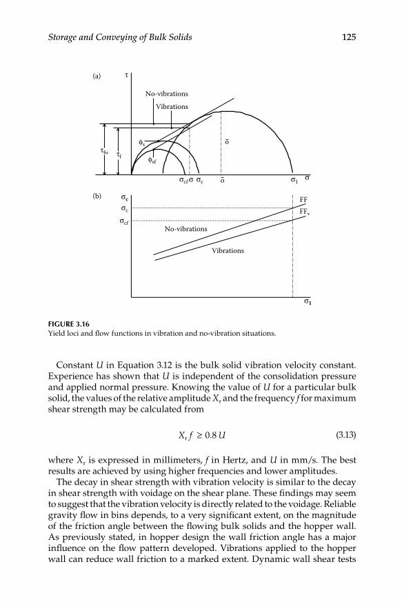
Storage and Conveying of Bulk Solids 125
Constant U in Equation 3.12 is the bulk solid vibration velocity constant. Experience has shown that U is independent of the consolidation pressure and applied normal pressure. Knowing the value of U for a particular bulk solid, the values of the relative amplitude Xr and the frequency f for maximum shear strength may be calculated from
X f Ur ≥ 0 8. (3.13)
where Xr is expressed in millimeters, f in Hertz, and U in mm/s. The best results are achieved by using higher frequencies and lower amplitudes.
The decay in shear strength with vibration velocity is similar to the decay in shear strength with voidage on the shear plane. These findings may seem to suggest that the vibration velocity is directly related to the voidage. Reliable gravity flow in bins depends, to a very significant extent, on the magnitude of the friction angle between the flowing bulk solids and the hopper wall. As previously stated, in hopper design the wall friction angle has a major influence on the flow pattern developed. Vibrations applied to the hopper wall can reduce wall friction to a marked extent. Dynamic wall shear tests
No-vibrations
(a)
(b)
τ
Vibrations
ϕsτfo
ϕsf
σcf
σcσc
σcf
σc σ1
σ1
σσ
oτf
o
No-vibrations
Vibrations
FFFFv
Figure 3.16Yield loci and flow functions in vibration and no-vibration situations.

126 Unit Operations of Particulate Solids
may be readily performed using the dynamic shear apparatus. The influence of mechanical vibration may induce flow by: (a) improving the mass-flow performance of an existing mass-flow bin by reducing the wall friction angle and critical arching dimension, (b) improving the funnel-flow performance of an existing funnel-flow bin by reducing the critical rathole dimension, (c) by lowering both the bulk strength and wall friction angle to convert an existing funnel-flow bin to a mass-flow bin.
Effective flow promotion depends on the ability of the stored bulk mass to transmit vibration energy to the region of the flow blockage. It is usual to install the vibrator on the hopper wall as to provide an immediate benefit through the resultant reduction in wall friction. If the flow blockage is in the form of an arch, vibration applied to the hopper wall at or near the outlet may cause the arch to fail and flow to occur. On the other hand, for stable ratholes, the vibration energy needs to be transmitted through the bulk mass in order to assist flow. The dynamic shear test apparatus, coupled with the theory of failure, provides information on the frequency and amplitude necessary to be applied at the zone of the flow blockage (Roberts et al., 1986). For best results, the higher modes of vibration should be used in flow promo-tion in order to create multiple tensile planes of failure as illustrated in Figure 3.17. Excitation frequencies in the order of 100 Hz, or higher, are necessary. Generally, the higher the frequency the higher the mode of vibration created in the bulk mass and, hence, the greater the number of failure zones. On the other hand, the vibration energy transmitted may have a higher attenuation at the higher excitation frequencies.
Air cannons or air blasters are also commonly used to promote gravity flow in bins. Terziovski and Arnold (1990) indicate that the sizing and placing of air blasters are normally carried out using techniques based on experience
TensionTension Tension
Compression
Silowall
(a)
(b)
Figure 3.17Formation of failure planes by vibration. (a) Static case and (b) dynamic case.
Storage and Conveying of Bulk Solids 127
and guesswork. Based on their own research on the use of air blasters, they provide a procedure for the correct selection of these devices for efficient performance using the measured flow properties of the bulk solid and the bin geometry. In general, air blasters are used in a retrofit situation to correct an inadequate design where flow blockages occur. However, in a new design where there is some uncertainty in the variations in bulk strength of a bulk solid for the full range of operating conditions, it is a good practice to make provision in the design for future installation of air blasters, in case it would become necessary.
3.3.7 Feeders for Discharge Control
In designing hoppers for silos, the procedure described so far would consist on making calculations to determine optimum hopper slope and outlet opening in order to ensure flow. In case flow does not occur, a flow promo-tion device can be selected after careful study of conditions and factors. Once flow out of a bin is guaranteed, the next step to complete the proper design of the bulk storage plant would consist on controlling the flow rate, as to provide adequate feed to any given food powder process. In order to do so, the use of a feeder will become necessary.
3.3.7.1 Feeders Description
A feeder is a device used to control the flow of bulk solids from a bin. Any feeder must be selected to suit a particular bulk solid and the range of feed rates required. It is particularly important to design the hopper and feeder as an integral unit, in order to ensure that the flow from the hopper is fully developed with uniform draw of material from the entire hopper outlet. There are several types of feeders but the most common are the belt or apron feeder, the screw feeder, the vibratory feeder, and the star feeder. Careful considerations, such as those described above, should be taken in selecting a feeder for a particular application.
An apron feeder consists on a conveyor belt positioned just below a tapered opening of a hopper. Due to the geometry of the conveyor, apron feeders are particularly suitable for slot opening hoppers. Care must be taken that dead spots are not produced in the flow channel above the feeder belt. The capacity of a belt feeder can be increased by tapering the outlet in the horizontal and vertical planes. In order to ensure proper flow of nonfree-flowing solids along the front bin wall, a sloping striker plate at the front of the hopper may be necessary. Belts have been used successfully under slot openings as long as 30 m with a constant slot width of 205 mm. Provisions should be made for field adjustment of the space between the skirt and the belt to provide uniform flow along the entire length. Since the minimum distance between the skirt and the belt should allow the largest particles to pass under, very long belt feeders are limited to the finer solids.

128 Unit Operations of Particulate Solids
A screw adapted to a hopper bin is known as a screw feeder. Screw feeders are quite useful in producing uniform feed rates for a variety of bilk solids. An important factor in this kind of feeder is the need for a variable pitch screw to produce a uniform draw of material across the entire hopper opening. For uniform flow to occur, the screw feeder opening-to-diameter ratio should not exceed a value of 6.
In a vibratory feeder, there is an inclined pan with different sort of motion located below a hopper opening. Vibratory feeders provide uniform flow along a slot opening of limited length. The distance between the feeder pan and the hopper is increased in the feed direction. Slot length is limited by the motion of the feeder. Because in long slots the upward component of motion is not relieved by the front opening, solids tend to pack. This can cause flow problems with sticky bulk materials, as well as large demand of power for free-flowing bulk solids. To overcome such difficulties, vibra-tory feeders and reciprocating-plate feeders are designed to feed across the slot. Although this type of feeder may require several drives to accom-modate extreme width, the drives are small due to the short length of the feeder.
Star feeders may provide highly uniform withdrawal along a slot hopper opening. They normally comprise six paddles whose ends converse in a common point forming a radial arrangement, or a six-point star when looking at its cross section. When the star rotates, withdrawal of bulk sol-ids is attained. A vertical section of at least one outlet width should be added above the feeder to ensure uniform discharge across the opening. Figure 3.18 presents schematic diagrams of the four types of feeders described, while Table 3.2 shows a preliminary guide for choosing a feeder.
3.3.7.2 Charge and Power Calculations
The estimation of feeders loads and drives powers requires knowledge of the stress fields generated in the hopper during the initial filling conditions, as well as during discharge. Under filling conditions, a peaked stress field is generated throughout the entire bin. As illustrated in Figure 3.19, once flow is initiated an arched stress field is generated in the hopper and a much greater proportion of the bin load is supported by the walls of the hopper. Consequently, the load acting on the feeder is reduced considerably. It is common for the load acting on the feeder under flow conditions to be in the order or 20% of the initial load. The arched stress field is quite stable and is maintained even if the flow is stopped. This means that once flow is initiated and then the feeder is stopped while the bin is still full, the arched stress field is retained and the load on the feeder remains at the reduced value. The load W on the feeder is given by
W q gL Bm m= − +ρb( ) ( )1 2
(3.14)
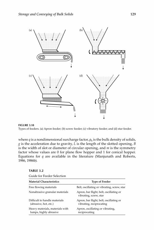
Storage and Conveying of Bulk Solids 129
where q is a nondimensional surcharge factor, ρb is the bulk density of solids, g is the acceleration due to gravity, L is the length of the slotted opening, B is the width of slot or diameter of circular opening, and m is the symmetry factor whose values are 0 for plane flow hopper and 1 for conical hopper. Equations for q are available in the literature (Manjunath and Roberts, 1986, 1986b).
(a) (b)
(c) (d)
Figure 3.18Types of feeders. (a) Apron feeder; (b) screw feeder; (c) vibratory feeder; and (d) star feeder.
Table 3.2
Guide for Feeder Selection
Material Characteristics Type of Feeder
Free flowing materials Belt, oscillating or vibrating, screw, star
Nonabrasive granular materials Apron, bar flight, belt, oscillating or vibrating, screw, star
Difficult to handle materials (abrasive, hot, etc.)
Apron, bar flight, belt, oscillating or vibrating, reciprocating
Heavy materials, materials with lumps, highly abrasive
Apron, oscillating or vibrating, reciprocating
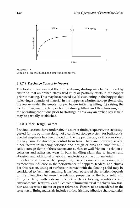
130 Unit Operations of Particulate Solids
3.3.7.3 Discharge Control in Feeders
The loads on feeders and the torque during start-up may be controlled by ensuring that an arched stress field fully or partially exists in the hopper prior to starting. This may be achieved by: (a) cushioning in the hopper, that is, leaving a quantity of material in the hopper as a buffer storage, (b) starting the feeder under the empty hopper before initiating filling, (c) raising the feeder up against the hopper bottom during filling and then lowering it to the operating conditions prior to starting; in this way an arched stress field may be partially established.
3.3.8 other Design Factors
Previous sections have underlain, in a sort of timing sequence, the steps sug-gested for the optimum design of a confined storage system for bulk solids. Special emphasis has been placed on the hopper design, as it is considered the key issue for discharge control from bins. There are, however, several other factors influencing selection and design of bins and silos for bulk solids storage. Some of these factors are: surface or wall friction in relation to cohesion and adhesion, wear in bulk handling plant due to impact and abrasion, and additional physical characteristics of the bulk material.
Friction and their related properties, like cohesion and adhesion, have tremendous influence in the performance of hoppers, feeders, and chutes. For this reason, lining of surfaces in contact with the flowing solid may be considered to facilitate handling. It has been observed that friction depends on the interaction between the relevant properties of the bulk solid and lining surface, with external factors such as loading conditions and environmental features. Careful choice of lining material to achieve low frac-tion and wear is a matter of great relevance. Factors to be considered in the selection of lining materials include surface friction, adhesive characteristics,
Feed
er lo
ad
EmptyingFilling
Time
Figure 3.19Load on a feeder at filling and emptying conditions.

Storage and Conveying of Bulk Solids 131
resistance to impact, anticorrosive properties, method of attachment, and cost. It is advisable to carry out appropriate tests to determine the relevant flow properties of the bulk solid and the proposed lining material. The fun-damental property of the solid to be considered would be the wall friction angle ϕ that can be determined as described in Section 2.4.3, or, alternatively, may be defined as follows:
ϕ τ
σ=
−tan 1
w (3.15)
where τ is the shear stress at wall surface and σw is the corresponding normal stress or pressure. The friction angle ϕ between the bulk solid and the bound-ary surface decreases as the normal pressure increases.
A common problem in bulk solids handling plants is the buildup of solids in surfaces of the discharging and conveying devices, due to cohesiveness and adhesiveness of the bulk solids being handled. If buildup is not con-trolled, blockages may eventually occur. In order to avoid buildup and blockages, it is necessary for the body forces generated in the bulk mass be sufficient to overcome the forces due to adhesion and shear. The body forces are normally those due to weight component of the bulk solid, but also may include inertia forces in dynamic systems such as in the case of belt conveyor discharge. The most suitable materials and the possibility of lining should be considered for feeders and chutes. In extreme cases, vibratory devices adapted to these components of the bulk solids handling plant, may be contemplated.
Wear of bulk solids handling plants is one of the major problems result-ing from routine processing activity. Wear may result from impact or abra-sion or, as is often the case, from a combination of both factors. Erosive type wear due to impact consists of plastic deformation and cutting wear. Excessive wear may occur in pipe bends of pneumatic conveying systems and at the discharge points of belt conveyors. Impact wear depends on fac-tors such as the relative hardness of the particles and the condition of the wall surface. Abrasive or rubbing wear occurs in storage bins and silos, particularly in hoppers, under mass-flow conditions. On such conditions, the pressures in a hopper will vary significantly over the whole surface, with the maximum pressure occurring at the transition and then decreas-ing toward the outlet. The velocity of the solids adjacent to the hopper wall increases nonlinearly from the transition to the outlet. The magnitude of the velocity at a particular point on the hopper wall depends on the bin discharge rate and the bulk solid velocities are low, with pure sliding tak-ing place. Abrasive wear also occurs in transfer chutes, feeders, belt con-veyors, vibratory conveyors, screw conveyors, and, in general, in any mechanical device involving the motion of bulk solids. Roberts et al. (1990) have suggested the use of a nondimensional Relative Wear Number NWR to

132 Unit Operations of Particulate Solids
allow for comparisons between the different bin and chute geometries. NWR is defined as
N
gBVVWR
w
b
s=
σρ ϕ
0tan
(3.16)
where σw is the normal pressure at boundary, ρb is the solid bulk density, g is the acceleration due to gravity, B is the outlet dimension of hopper or chute width, Vs is the velocity at the sliding wall, V0 is the sliding velocity at a refer-ence location, and ϕ is the wall friction angle.
Some other characteristics of the bulk solids can affect design and flowing capacity in a bulk solids handling plant. In terms of particle size, bulk solids will flow better at a coarser range of particle sizes and with minimum pres-ence of fines. Conditioning by agglomeration or any other process in order to minimize fines and improve flowability, is sometimes carried out in bulk solids handling plants. The alternative may be, however, time consuming and economically unfeasible. The moisture affects flow, with bulk solids flowing better at lower moisture content. Many inert industrial powders can absorb water up to a certain point, before presenting severe flow problems. Biological materials can be better water absorbents and may cause flow prob-lems, unless a treatment, like drying, is included in their handling. The cost incurred in drying may be offset by improving flow, minimizing shipping costs, and controlling deterioration losses. Moisture content can also be con-trolled by substituting the air in the voidage of the bed of stored particles, by a dry stable gas such as nitrogen. Regarding temperature, the flow may become difficult at high temperatures, mostly in biological materials that may release sticky substances of low melting points. In this case, a cooling system may be necessary to maintain stored solids free from releasing sub-stances. As with the drying alternative previously mentioned, consideration should be given to the possible compensation of the cost of cooling, in terms of flow improvement and some other advantages, such as quality preserva-tion of the stored material. Storing time may also affect flowability as attri-tion and erosion may smooth sharp edges of polyhedral particles rounding them and facilitating their flow.
As a final part of design factors in a bulk solids handling plant, ancillary accessories like gates and level gauges may be taken into account. Gates are used to control release of flow from bins and hoppers to feeders or conveyors. There are several gate designs, such as the hand-slide gate, the lever- operated quadrant gate, and the rack-and-pinion gate. The hand-slide gate could be, in fact, quite difficult to operate by hand, and so it is restricted to low-capacity vessels and light bulk solids. The lever-operated quadrant gate is not used to control the flow, but rather to allow the free discharge of lumpy materials with a quick opening turn. The rack-and-pinion gate is the most sophisti-cated design of the three gates listed. It is considered a precision gate, which is usually tightly sealed against dust and dribble, and can be operated either
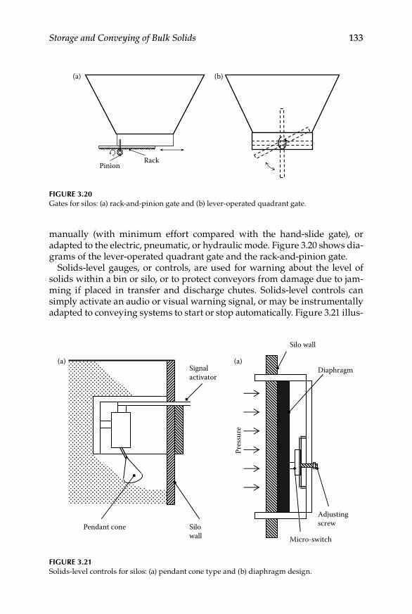
Storage and Conveying of Bulk Solids 133
manually (with minimum effort compared with the hand-slide gate), or adapted to the electric, pneumatic, or hydraulic mode. Figure 3.20 shows dia-grams of the lever-operated quadrant gate and the rack-and-pinion gate.
Solids-level gauges, or controls, are used for warning about the level of solids within a bin or silo, or to protect conveyors from damage due to jam-ming if placed in transfer and discharge chutes. Solids-level controls can simply activate an audio or visual warning signal, or may be instrumentally adapted to conveying systems to start or stop automatically. Figure 3.21 illus-
PinionRack
(a) (b)
Figure 3.20Gates for silos: (a) rack-and-pinion gate and (b) lever-operated quadrant gate.
Pendant cone Silowall
Signalactivator
Pres
sure
Silo wall
(a) (a)Diaphragm
Micro-switch
Adjustingscrew
Figure 3.21Solids-level controls for silos: (a) pendant cone type and (b) diaphragm design.

134 Unit Operations of Particulate Solids
trates two types of solids-level controls: the pendant cone level controller and the diaphragm level control unit.
3.4 Laboratory Exercise: Evaluation of Wall Loads in Silos
3.4.1 introduction
Silo design has been a big concern since the end of the nineteenth century. The physical phenomenon arising from the interactions between confined solids and the walls of its storage structures is poorly understood. The starting point to design may be the calculation of pressure of silo walls at different depths in order to choose silo building materials, structural sup-ports, and so on. The original theory of Janssen to estimate pressure on silo walls has been generally accepted and perfected over the years. This theory describes the friction between a layer of grain and the silo wall and estab-lishes the static two-dimensional mathematical equilibrium of the vertical forces. From the established vertical forces, the vertical pressure, and thus the horizontal pressures, can be obtained. The objective of the experiment is to calculate pressure loads on a model grain silo at different heights as to corroborate the applicability of Janssen’s equation.
3.4.2 equipment and Materials
A small-scale metal silo (1–1.2 m height and 0.5–0.6 m diameter) can be used for the experiment. The material to be stored can be any kind of available grain, like wheat or barley.
3.4.3 instruments and apparatuses
Strain gauges or pressure cells and electronic wall pressure indicator.
3.4.4 Procedure
Characterize the grain in terms of its main physical properties, such •as bulk density and angle of repose.Fix the strain gauges at different (at least four) equally spaced dis-•tances along the height of the silo.Connect the gauges to the electronic pressure indicator.•Fill up the silo to its complete height.•Record the pressure at the different levels and at different times, for •example, immediately after filling the silo, 1 h after filling, several hours after filling, and 24 h after filling.
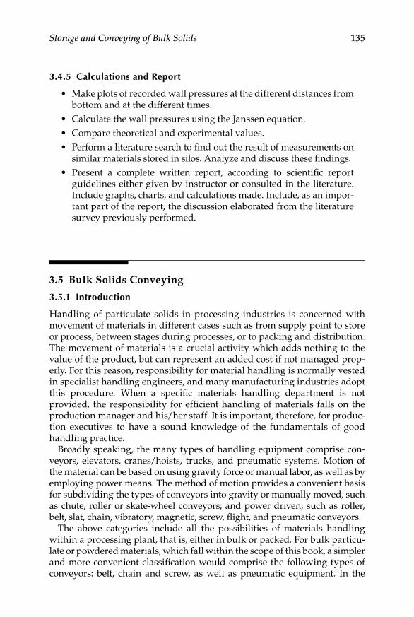
Storage and Conveying of Bulk Solids 135
3.4.5 Calculations and report
Make plots of recorded wall pressures at the different distances from •bottom and at the different times.Calculate the wall pressures using the Janssen equation.•Compare theoretical and experimental values.•Perform a literature search to find out the result of measurements on •similar materials stored in silos. Analyze and discuss these findings.Present a complete written report, according to scientific report •guidelines either given by instructor or consulted in the literature. Include graphs, charts, and calculations made. Include, as an impor-tant part of the report, the discussion elaborated from the literature survey previously performed.
3.5 Bulk Solids Conveying
3.5.1 introduction
Handling of particulate solids in processing industries is concerned with movement of materials in different cases such as from supply point to store or process, between stages during processes, or to packing and distribution. The movement of materials is a crucial activity which adds nothing to the value of the product, but can represent an added cost if not managed prop-erly. For this reason, responsibility for material handling is normally vested in specialist handling engineers, and many manufacturing industries adopt this procedure. When a specific materials handling department is not provided, the responsibility for efficient handling of materials falls on the production manager and his/her staff. It is important, therefore, for produc-tion executives to have a sound knowledge of the fundamentals of good handling practice.
Broadly speaking, the many types of handling equipment comprise con-veyors, elevators, cranes/hoists, trucks, and pneumatic systems. Motion of the material can be based on using gravity force or manual labor, as well as by employing power means. The method of motion provides a convenient basis for subdividing the types of conveyors into gravity or manually moved, such as chute, roller or skate-wheel conveyors; and power driven, such as roller, belt, slat, chain, vibratory, magnetic, screw, flight, and pneumatic conveyors.
The above categories include all the possibilities of materials handling within a processing plant, that is, either in bulk or packed. For bulk particu-late or powdered materials, which fall within the scope of this book, a simpler and more convenient classification would comprise the following types of conveyors: belt, chain and screw, as well as pneumatic equipment. In the

136 Unit Operations of Particulate Solids
literature all these forms of bulk material movement are known as conveyors and, thus, a proper categorization of the handling equipment for bulk par-ticulate food solids would comprise the following groups: (a) belt conveyors; (b) chain conveyors: scraper conveyors, apron conveyors and bucket eleva-tors; (c) screw conveyors; and (d) pneumatic conveyors: dense phase systems and dilute phase systems.
The above classification groups the different types of conveying systems in virtue of their operating principle. For example, regardless of whether a bulk material is being moved horizontally, inclined, or vertically, chain conveying can perform the duty based on the same principle of fixing an element (a paddle or a bucket) to a system of chains externally powered.
Bulk solids conveying represents one of those disciplines which have been neglected in terms of scientific research and development, when compared with other operations in particle technology directly related to processing, such as attrition or agglomeration. Conveying systems and supplies are normally provided by a large, capable manufacturing industry, which holds much of the engineering information in form of brochures, data sheets, and nomographs. Tables 3.3 and 3.4 present a general guide on conveying sys-tems selection.
3.5.2 belt Conveyors
The belt conveyor consists, essentially, of an endless belt operating between two or more pulleys, friction driven at one end and carried on an idler drum at the opposite end. Belt conveyors are used for movement of different types of bulk solids at distances varying from meters to kilometers and, thus, the belt and its load have to be supported on idlers on both conveying and return sections. Heavy-duty machines also have thick belts and these require larger diameter idler end drums. The construction of a belt conveying system requires a support structure, usually of steelwork. Belt conveyors have a high mechanical efficiency since, in larger installations, all the load is carried on antifriction bearings. Damage to the product in movement is slight because there is little or no relative motion, between the product being transported and the belt. The carrying capacity is high since relatively high speeds are possible when the whole system is operating. Bulk solid materials can be car-ried long distances mainly in horizontal plane, although there is a possibility of inclined conveying with certain limit to the angle of elevation. Inclination is usually limited to 15° or 20° and, in order to avoid excess spillage or “run-back,” special belts with corrugated sidewalks and lateral ribs are used for steeper inclination, up to a nominal 45°. A properly designed and maintained belt system has a long service life, but the initial cost is usually high, so installation is only advisable when amortization of the high initial cost can be assured.
The elements comprising a belt conveying system are: the belt, a drive system, some tension elements, the idlers, and appropriate loading and

Storage and Conveying of Bulk Solids 137
Tab
le 3
.3
Mai
n Fe
atu
res
of D
iffe
rent
Con
veyi
ng S
yste
ms
Sys
tem
Dir
ecti
onFr
equ
ency
Loc
atio
nS
ervi
ceH
eigh
tM
ater
ial S
tate
Vertical upward
Vertical downward
Inclined upward
Inclined downward
Horizontal
Continuous
Noncontinuous
Occasional
Spot
Path
Limited area
Unlimited area
Permanent
Temporary
Nondefined
Over head
Head level
Ground level
Underground
Packed
Bulk
Solid
Liquid
Con
veyo
rx
xx
xx
xx
xx
xx
xx
Ele
vato
rx
xx
xx
xx
xx
xC
rane
xx
xx
xx
xx
xx
xx
Truc
kx
xx
xx
xx
xx
xPn
eum
atic
xx
xx
xx
xx
xx
xx
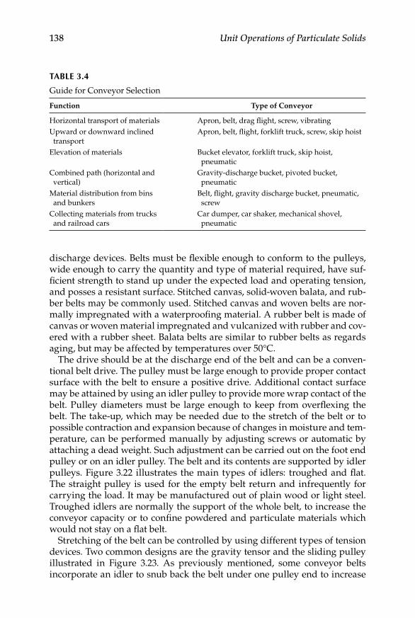
138 Unit Operations of Particulate Solids
discharge devices. Belts must be flexible enough to conform to the pulleys, wide enough to carry the quantity and type of material required, have suf-ficient strength to stand up under the expected load and operating tension, and posses a resistant surface. Stitched canvas, solid-woven balata, and rub-ber belts may be commonly used. Stitched canvas and woven belts are nor-mally impregnated with a waterproofing material. A rubber belt is made of canvas or woven material impregnated and vulcanized with rubber and cov-ered with a rubber sheet. Balata belts are similar to rubber belts as regards aging, but may be affected by temperatures over 50°C.
The drive should be at the discharge end of the belt and can be a conven-tional belt drive. The pulley must be large enough to provide proper contact surface with the belt to ensure a positive drive. Additional contact surface may be attained by using an idler pulley to provide more wrap contact of the belt. Pulley diameters must be large enough to keep from overflexing the belt. The take-up, which may be needed due to the stretch of the belt or to possible contraction and expansion because of changes in moisture and tem-perature, can be performed manually by adjusting screws or automatic by attaching a dead weight. Such adjustment can be carried out on the foot end pulley or on an idler pulley. The belt and its contents are supported by idler pulleys. Figure 3.22 illustrates the main types of idlers: troughed and flat. The straight pulley is used for the empty belt return and infrequently for carrying the load. It may be manufactured out of plain wood or light steel. Troughed idlers are normally the support of the whole belt, to increase the conveyor capacity or to confine powdered and particulate materials which would not stay on a flat belt.
Stretching of the belt can be controlled by using different types of tension devices. Two common designs are the gravity tensor and the sliding pulley illustrated in Figure 3.23. As previously mentioned, some conveyor belts incorporate an idler to snub back the belt under one pulley end to increase
Table 3.4
Guide for Conveyor Selection
Function Type of Conveyor
Horizontal transport of materials Apron, belt, drag flight, screw, vibratingUpward or downward inclined transport
Apron, belt, flight, forklift truck, screw, skip hoist
Elevation of materials Bucket elevator, forklift truck, skip hoist, pneumatic
Combined path (horizontal and vertical)
Gravity-discharge bucket, pivoted bucket, pneumatic
Material distribution from bins and bunkers
Belt, flight, gravity discharge bucket, pneumatic, screw
Collecting materials from trucks and railroad cars
Car dumper, car shaker, mechanical shovel, pneumatic

Storage and Conveying of Bulk Solids 139
friction and minimize sliding of the belt over the pulley, and such arrange-ment can also be considered a tension device.
The material can be fed onto the belt by hand or by a mechanism provid-ing continuous and steady flow. This may be a simple hopper with a gate valve or, if the material is not free flowing, coupled to an apron, screw, vibrat-ing, or any other type of feeder. The material may be discharged over the end of the belt, by a diagonal scraper, by titling one or more of the idler pulleys, or by a tripper. As shown in Figure 3.24, a tripper consists of two idler pulleys mounted in such a way that cause the belt to take the shape of an S.
Flat belt (return)
Troughed belt(loaded)
Troughedidlers
Flat idlers
Figure 3.22Idler pulleys for belt conveyors.
(a) (b)
Figure 3.23Tensors for belt conveyors: (a) gravity tensor and (b) sliding pulley.
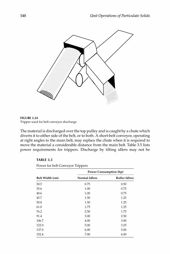
140 Unit Operations of Particulate Solids
The material is discharged over the top pulley and is caught by a chute which diverts it to either side of the belt, or to both. A short-belt conveyor, operating at right angles to the main belt, may replace the chute when it is required to move the material a considerable distance from the main belt. Table 3.5 lists power requirements for trippers. Discharge by tilting idlers may not be
Figure 3.24Tripper used for belt conveyor discharge.
Table 3.5
Power for belt Conveyor Trippers
Belt Width (cm)
Power Consumption (hp)
Normal Idlers Roller Idlers
30.5 0.75 0.5035.6 1.00 0.7540.6 1.00 0.7545.7 1.50 1.2550.8 1.50 1.2561.0 1.75 1.2576.2 2.50 1.7591.4 3.00 2.50106.7 4.00 3.00122.0 5.00 3.25137.0 6.00 5.00152.4 7.00 6.00

Storage and Conveying of Bulk Solids 141
advisable since the material is discharged over a considerable length of the belt and there is an additional strain placed upon the belt due to twisting. An angle scraper is the simplest discharging device and provides satisfactory discharge for many materials. The various discharge systems are designed so that they may be controlled remotely.
A large belt conveyor system is an expensive an intricate facility which should be designed and installed under the supervision of specially trained conveyor engineers. During the last decades, the knowledge about belt conveyor design has been enriched and new design procedures have been proposed based on the capabilities offered by modern computer systems. Foote et al. (1988) examine the payoff of simulation and network analysis in conveyor system design, while Roberts (1994) presents an overview of tech-nical and economical factors involved in conveyor design. Belt conveying design is far from standardized, and the following suggestions are only intended for preliminary approximations and calculations.
The horsepower required for movement of material by belt conveyors can be calculated by conventional engineering methods by considering the fric-tional resistance of the belt, the lift, and the frictional resistance of the differ-ent pulleys and trippers. However, the constants used in such procedure may vary with change in operating conditions. Also, flexing of the load and belt between supporting pulleys absorbs some energy. Power for standard installations can be consulted in tabulated data or, alternatively, calculated from the following equations:
Power to drive empty conveyor:
P
F L L W=
+( )( . )0 0 06270
v
(3.17)
Power to convey material on level:
P
F L L T=
+( )0
270 (3.18)
Power to lift material:
P
TH=270
(3.19)
Power to operate a tripper:
P Y ZT= +v (3.20)
where P is the power in horsepower, F is a friction factor taking values between 0.03 and 0.05, L is the conveyor length in meters, L0 is a constant tak-ing values between 30.5 and 45.7, W is the weight of all moving parts of the conveyor in kilograms per meter of overall length, v is the conveyor speed in m/min, T is the conveyor capacity in tons/h, and H is the height of lift in
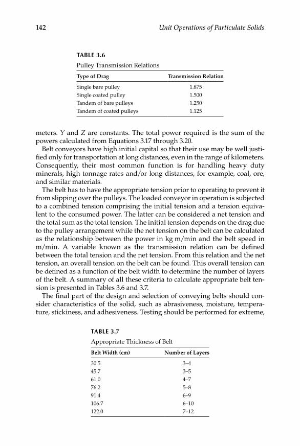
142 Unit Operations of Particulate Solids
meters. Y and Z are constants. The total power required is the sum of the powers calculated from Equations 3.17 through 3.20.
Belt conveyors have high initial capital so that their use may be well justi-fied only for transportation at long distances, even in the range of kilometers. Consequently, their most common function is for handling heavy duty minerals, high tonnage rates and/or long distances, for example, coal, ore, and similar materials.
The belt has to have the appropriate tension prior to operating to prevent it from slipping over the pulleys. The loaded conveyor in operation is subjected to a combined tension comprising the initial tension and a tension equiva-lent to the consumed power. The latter can be considered a net tension and the total sum as the total tension. The initial tension depends on the drag due to the pulley arrangement while the net tension on the belt can be calculated as the relationship between the power in kg m/min and the belt speed in m/min. A variable known as the transmission relation can be defined between the total tension and the net tension. From this relation and the net tension, an overall tension on the belt can be found. This overall tension can be defined as a function of the belt width to determine the number of layers of the belt. A summary of all these criteria to calculate appropriate belt ten-sion is presented in Tables 3.6 and 3.7.
The final part of the design and selection of conveying belts should con-sider characteristics of the solid, such as abrasiveness, moisture, tempera-ture, stickiness, and adhesiveness. Testing should be performed for extreme,
Table 3.6
Pulley Transmission Relations
Type of Drag Transmission Relation
Single bare pulley 1.875Single coated pulley 1.500Tandem of bare pulleys 1.250Tandem of coated pulleys 1.125
Table 3.7
Appropriate Thickness of Belt
Belt Width (cm) Number of Layers
30.5 3–445.7 3–561.0 4–776.2 5–891.4 6–9106.7 6–10122.0 7–12
Storage and Conveying of Bulk Solids 143
rather than average conditions, to verify appropriate tension and other oper-ating conditions of the conveyor.
Alternative designs to the conventional belt conveyors include steep-angle and vertical conveying systems with the surface worked into pockets formed by high sidewalls and scoop cleats, and hose-belt or tube conveyors in which the flat belt is shaped by means of concave idlers and guide rollers to overlap the belt edges (Bahke, 1991).
example 3.3
Calculate the power to move a load of 850 tons/h of a granular material on a conveyor belt, 1 m wide and 100 m long. The conveyor operates at 150 m/min and its moving parts weight 5000 kg approximately. Constants F and L0 have been evaluated as 0.04 and 38, respectively.
SoluTion
The overall power will include the power to operate the empty conveyor and the power to move the load. Equation 3.17 is used to calculate the power of the empty conveyor while Equation 3.18 is used to calculate the power needed to actually convey the load. Constant 0.06 on those equations is expressed in ton min/kg h, and constant 270 is expressed in ton m/hp h. The remaining constants are dimen-sionless. Substituting values in Equation 3.17 for the empty conveyor:
P = + =0 04 100 38 0 06 50 150
270. ( )[( . )( )( )]
.9 2 hp
For the load, using Equation 3.18:
P = + =0 04 100 38 850
270. ( )( )
.17 4 hp
The overall power will, therefore, be 26.6 hp.
3.5.3 Chain Conveyors
Compared to belt conveying systems, chain conveyors present a series of con-trasting characteristics such as cheaper construction, noisy operation, slower movement, mechanic inefficiency, and no specialized skill required for their design. Chain conveyors are very versatile in design being more easily adapt-able to different duties than belt conveyors. The main components of these types of conveying systems are the chains, the moving elements, and the drives. The types of chain available for conveying are extremely varied and a simple complete classification would be difficult to provide. Types of chain commonly used in chain conveyors are the malleable detachable, malleable pintle, steel, roller, and combination. The malleable detachable chain is, pos-sibly, the most common and is normally used for light intermittent service.
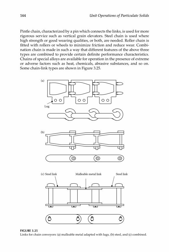
144 Unit Operations of Particulate Solids
Pintle chain, characterized by a pin which connects the links, is used for more rigorous service such as vertical grain elevators. Steel chain is used where high strength or good wearing qualities, or both, are needed. Roller chain is fitted with rollers or wheels to minimize friction and reduce wear. Combi-nation chain is made in such a way that different features of the above three types are combined to provide certain definite performance characteristics. Chains of special alloys are available for operation in the presence of extreme or adverse factors such as heat, chemicals, abrasive substances, and so on. Some chain-link types are shown in Figure 3.25.
Lug
Steel link Malleable metal link Steel link
(a)
(b)
(c)
Figure 3.25Links for chain conveyors: (a) malleable metal adapted with lugs, (b) steel, and (c) combined.
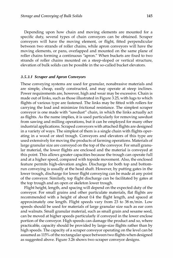
Storage and Conveying of Bulk Solids 145
Depending upon how chain and moving elements are mounted for a specific duty, several types of chain conveyors can be obtained. Scraper conveyors will have the moving element, or flight, fitted perpendicular between two strands of roller chains, while apron conveyors will have the moving elements, or pans, overlapped and mounted on the same plane of roller chains forming a continuous “apron.” When buckets are fixed to two strands of roller chains mounted on a steep-sloped or vertical structure, elevation of bulk solids can be possible in the so-called bucket elevators.
3.5.3.1 Scraper and Apron Conveyors
These conveying systems are used for granular, nonabrasive materials and are simple, cheap, easily constructed, and may operate at steep inclines. Power requirements are, however, high and wear may be excessive. Chain is made out of links, such as those illustrated in Figure 3.25, with lugs to which flights of various type are fastened. The links may be fitted with rollers for carrying the load and minimize frictional resistance. The simplest scraper conveyor is one made with “sawdust” chain, in which the links actually act as flights. As the name implies, it is used particularly for removing sawdust from sawing and milling operations, but it can be employed for many other industrial applications. Scraped conveyors with attached flights are designed in a variety of ways. The simplest of them is a single chain with flights oper-ating in a wood or steel trough. Conveyors and elevators of this type are used extensively for moving the products of farming operations. Materials of large granular size are conveyed on the top of the conveyor. For small granu-lar material, the lower flights are enclosed and the material is conveyed at this point. This allows greater capacities because the trough can operate full and at a higher speed, compared with topside movement. Also, the enclosed feature permits high-elevation angles. Discharge for both top and bottom-run conveying is usually at the head shaft. However, by putting gates in the lower trough, discharge for lower flight conveying can be made at any point of the conveyor. Similarly, top flight discharge can be facilitated by gates at the top trough and an open or skeleton lower trough.
Flight height, length, and spacing will depend on the expected duty of the conveyor. For small grains and other particulate materials, flat flights are recommended with a height of about 0.4 the flight length, and spaced at approximately one length. Flight speeds vary from 23 to 38 m/min. Low speeds should be used for materials of large granular size such as ear corn and walnuts. Small granular material, such as small grain and sesame seed, can be moved at higher speeds particularly if conveyed in the lower enclose portion of the conveyor. High speeds can damage the product and so, where practicable, capacity should be provided by large-size flights rather than by high speeds. The capacity of a scraper conveyor operating on the level can be assumed as 115% of the rectangular space between two flights when designed as suggested above. Figure 3.26 shows two scraper conveyor designs.
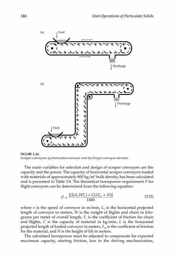
146 Unit Operations of Particulate Solids
The main variables for selection and design of scraper conveyors are the capacity and the power. The capacity of horizontal scraper conveyors loaded with materials of approximately 800 kg/m3 bulk density, has been calculated and is presented in Table 3.8. The theoretical horsepower requirement P for flight conveyors can be determined from the following equation:
P
vL WF C LF H= + +[( ) ( )]21400
c c m
(3.21)
where v is the speed of conveyor in m/min, Lc is the horizontal projected length of conveyor in meters, W is the weight of flights and chain in kilo-grams per meter of overall length, Fc is the coefficient of friction for chain and flights, C is the capacity of material in kg/min, L is the horizontal projected length of loaded conveyor in meters, Fm is the coefficient of friction for the material, and H is the height of lift in meters.
The calculated horsepower must be adjusted to compensate for expected maximum capacity, starting friction, loss in the driving mechanization,
Discharge
Feed
Discharge
Feed
(a)
(b)
Figure 3.26Scraper conveyors: (a) horizontal conveyor and (b) Z-type conveyor-elevator.

Storage and Conveying of Bulk Solids 147
variation in friction coefficients, type of power unit, and so on. The value of the coefficient Fc for chain dragging on metal can be taken as 0.33, while that for chain over wood can be approximated to 0.6. Friction coefficients for different materials are listed in Table 3.9.
For roller chains, Fc can be calculated from the following expression:
F X
dD
YDc = + + 2
(3.22)
Table 3.8
Capacity of Scraper Conveyorsa,b,c
Flight Size (cm) Flight Weight (kg)
10 × 25.4 6.80
10 × 30.5 8.62
12.7 × 30.5 10.43
12.7 × 38.1 14.06
15.24 × 45.7 18.14
20.30 × 45.7 27.21
20.30 × 50.8 31.75
20.30 × 61.0 40.82
25.40 × 61.0 52.16
a For 800 kg/m3 bulk density material and conveyor velocity of 30 m/min.
b For different density materials, capacity proportional to weight per cubic meter of material.
c Capacity of inclined conveyor compared with horizontal one:
Slope Degrees
Percent Capacity of Horizontal
20 7730 5540 33
Table 3.9
Friction Coefficient for Various Materials Sliding on Metal
Material Fm
Bituminous coal 0.590Anthracite 0.330Coke 0.355Damp ashes 0.530Dry sand 0.600Limestone 0.585
148 Unit Operations of Particulate Solids
where X is a constant (0.33 for metal on nonlubricated metal, and 0.2 for metal on lubricated metal), d is the diameter of the rod on which the roller rotates, D the roller diameter, and Y is a constant whose value can be taken as 0.03 for general purposes.
For inclined conveyors, the power can be calculated from
P WL F W L F WL F= + + + + −c m c c c msin sin sin( cos ) ( cos ) ( cos )α α α α α α1 (3.23)
where α is the slope angle and W1 is the load in kg per overall length of conveyor.
If the flights in the scraper conveyors are replaced with flat slats, steel plates or boards, a moving platform or apron is obtained and can be used for movement of sacked or large unit-sized materials. The typical design is a series of pans mounted between two strands of roller chain, with pans overlapping to eliminate dribble, and often equipped with end plates for deeper loads. Apron conveyors are not suitable for conveying of powdered and particulate materials. For such materials, their main application is feed-ing at controlled rates, with lump sizes large enough to minimize dribbling. Apron-feeder applications range from fairly light duties with light-gauge steel pans, up to extremely heavy duties requiring reinforced manganese steel pans with center supports. Capacity and power of apron conveyors can be found in tables and design graphs reported on text books (Badger and Banchero, 1955; Green and Perry, 2008).
3.5.3.2 Bucket Elevators
This type of conveying comprises high-capacity units primarily intended for bulk elevation of relatively free-flowing materials and may be considered a special adaptation of chain conveying. Bucket elevators are the simplest and most dependable equipment units for vertical lifting of different types of granular materials. They are available in a wide range of capacities and may operate either in the entire open or be totally enclosed. High efficiency in bucket elevators results from the absence of frictional loss from sliding of the material on the housing, and this feature distinguishes it from the vertical, or nearly vertical, scraper conveyor. The material carrying element of this sort of conveying is the bucket, which may be enclosed in a single housing called a leg, or two legs may be used. The return leg may be located some distance from the elevator leg. A single or double chain is used to attach the buckets. The more important considerations affecting the design and opera-tion of bucket elevators are: (a) the physical properties of the conveyed mate-rial, (b) the shape and spacing of the buckets, (c) the speed at which the elevator is driven, (d) the method of loading the elevator, and (e) the method of discharging the elevator.
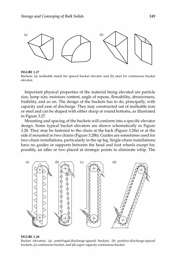
Storage and Conveying of Bulk Solids 149
Important physical properties of the material being elevated are particle size, lump size, moisture content, angle of repose, flowability, abrasiveness, friability, and so on. The design of the buckets has to do, principally, with capacity and ease of discharge. They may constructed out of malleable iron or steel and can be shaped with either sharp or round bottoms, as illustrated in Figure 3.27.
Mounting and spacing of the buckets will conform into a specific elevator design. Some typical bucket elevators are shown schematically in Figure 3.28. They may be fastened to the chain at the back (Figure 3.28a) or at the side if mounted in two chains (Figure 3.28b). Guides are sometimes used for two-chain installations, particularly in the up leg. Single-chain installations have no guides or supports between the head and foot wheels except for, possibly, an idler or two placed at strategic points to eliminate whip. The
(a) (b) (c) (d)
Figure 3.28Bucket elevators: (a) centrifugal-discharge-spaced buckets, (b) positive-discharge-spaced buckets, (c) continuous bucket, and (d) super capacity continuous bucket.
(a) (b)
Figure 3.27Buckets: (a) malleable metal for spaced bucket elevator and (b) steel for continuous bucket elevator.

150 Unit Operations of Particulate Solids
center spacing of buckets varies with their size, shape, speed, as well as head and foot wheel diameter. The buckets must be placed so that the centrifugal discharging grain does not hit the bucket ahead of the one dis-charging. For general purposes, the spacing will be from 2 to 3 times the projected width.
As shown diagrammatically in Figure 3.28, bucket elevators can be mainly loaded in three different ways. Spaced buckets receive part of the charge directly from a chute and part by scooping (Figure 3.28a), continuous buck-ets are filled as they pass through a loading leg with a feed spout above the tail wheel (Figure 3.28b) and, also, they can be loaded in a bottomless boot with a cleanout door (Figure 3.28c). In terms of discharge, spaced-bucket centrifugal-discharge elevators (Figure 3.28a) are the most common and are usually equipped with malleable-iron round-shaped buckets (Figure 3.27) spaced to prevent interference in loading or discharge. This type of elevator will handle almost any free-flowing fine or small-lump material. Speeds can be relatively high for fairly dense materials, but must be lowered consid-erably for aerated or low bulk-density materials to prevent fanning action. Spaced-bucket positive-discharge elevators (Figure 3.28b) are essentially the same as centrifugal-discharge units, except that the buckets are mounted on two strands of chain and are snubbed back under the head sprocket to invert them to allow positive discharge. These units are designed especially for materials which are sticky or tend to pack, and the slight impact of the chain seating on the snub sprocket, combined with complete bucket inversion, is generally sufficient to empty the buckets completely. Continuous-bucket elevators (Figure 3.28c) are generally used for larger-lump materials or for materials too difficult to handle with centrifugal-discharge elevators. Buckets used are of the steel type, such as those illustrated in Figure 3.27. They are closely spaced and the back of the preceding one serves as a discharge chute for the bucket which is dumping as it rounds the head pulley. Close bucket spacing reduces the speed at which the elevator oper-ates to maintain capacities comparable with the spaced-bucket units. Gentle discharge is, therefore, promoted to help preventing excessive degradation and making this type of elevator suitable for handling finely pulverized or aerated materials. Super-capacity continuous-bucket elevators (Figure 3.28c) are designed for high lifts and large-lump material. They handle high tonnages and are usually operated at an incline to improve loading, as well as discharge conditions. Running speeds are low and, due to the heavy loads, bucket-supporting chain is usually guided on the elevating and return parts.
Bucket elevator horsepower for spaced buckets and digging boots can be calculated using the following equation:
P
TH=152
(3.24)
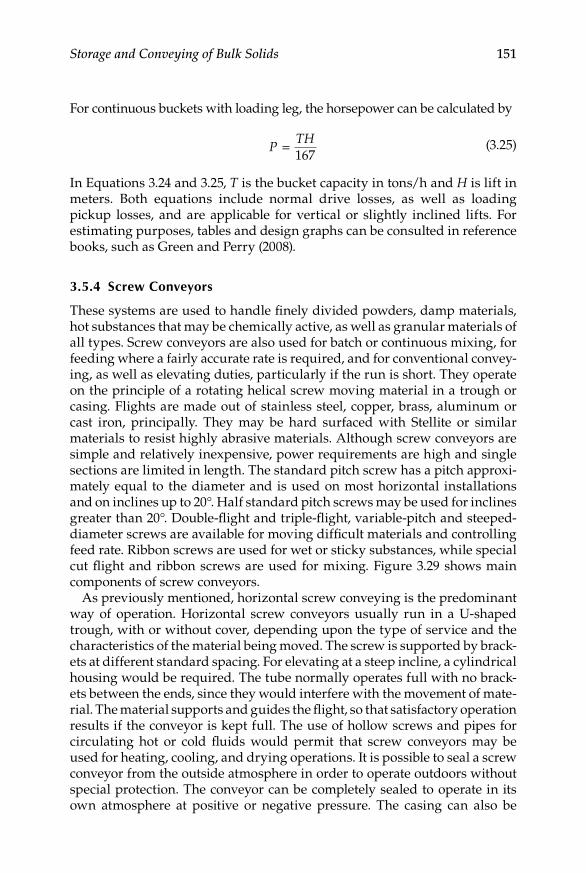
Storage and Conveying of Bulk Solids 151
For continuous buckets with loading leg, the horsepower can be calculated by
P
TH=167
(3.25)
In Equations 3.24 and 3.25, T is the bucket capacity in tons/h and H is lift in meters. Both equations include normal drive losses, as well as loading pickup losses, and are applicable for vertical or slightly inclined lifts. For estimating purposes, tables and design graphs can be consulted in reference books, such as Green and Perry (2008).
3.5.4 Screw Conveyors
These systems are used to handle finely divided powders, damp materials, hot substances that may be chemically active, as well as granular materials of all types. Screw conveyors are also used for batch or continuous mixing, for feeding where a fairly accurate rate is required, and for conventional convey-ing, as well as elevating duties, particularly if the run is short. They operate on the principle of a rotating helical screw moving material in a trough or casing. Flights are made out of stainless steel, copper, brass, aluminum or cast iron, principally. They may be hard surfaced with Stellite or similar materials to resist highly abrasive materials. Although screw conveyors are simple and relatively inexpensive, power requirements are high and single sections are limited in length. The standard pitch screw has a pitch approxi-mately equal to the diameter and is used on most horizontal installations and on inclines up to 20°. Half standard pitch screws may be used for inclines greater than 20°. Double-flight and triple-flight, variable-pitch and steeped-diameter screws are available for moving difficult materials and controlling feed rate. Ribbon screws are used for wet or sticky substances, while special cut flight and ribbon screws are used for mixing. Figure 3.29 shows main components of screw conveyors.
As previously mentioned, horizontal screw conveying is the predominant way of operation. Horizontal screw conveyors usually run in a U-shaped trough, with or without cover, depending upon the type of service and the characteristics of the material being moved. The screw is supported by brack-ets at different standard spacing. For elevating at a steep incline, a cylindrical housing would be required. The tube normally operates full with no brack-ets between the ends, since they would interfere with the movement of mate-rial. The material supports and guides the flight, so that satisfactory operation results if the conveyor is kept full. The use of hollow screws and pipes for circulating hot or cold fluids would permit that screw conveyors may be used for heating, cooling, and drying operations. It is possible to seal a screw conveyor from the outside atmosphere in order to operate outdoors without special protection. The conveyor can be completely sealed to operate in its own atmosphere at positive or negative pressure. The casing can also be

152 Unit Operations of Particulate Solids
insulated to maintain internal temperatures in areas or extreme ambient temperatures. The casing can be designed with a drop bottom for easy clean-ing to avoid contamination when different materials are to be conveyed through the same system.
Screw conveyors are usually made up of standard sections coupled together, and so special attention should be given to bending stresses in the couplings. Hanger bearings supporting the flights can obstruct the flow of material when the trough is loaded above its level. Thus, with difficult mate-rials, the load in the trough must be kept below this level. Alternatively, special hanger bearings which minimize obstruction should be selected. Since screw conveyors operate at relatively low rotational speeds, the fact that the outer edge of the flight may be moving at a relatively high linear speed is often neglected. This may create a wear problem, and if wear is too severe it can be reduced by the use of hard-surfaced edges, detachable hard-ened flight segments, rubber covering, or high-carbon steels. Screw convey-ors are well suited as feeders or metering devices under bins or hoppers. The portion of the screw under the container is usually designed with half or third pitch, the balance of the screw full pitch. Thus, the main portion of the screw operates half or third full, while the metering portion of the screw operates full.
(a)
(c)
(b)
Figure 3.29Screw conveyor components: (a) flight, (b) screw formed by mounting flights on an axle, and (c) trough.

Storage and Conveying of Bulk Solids 153
Concise data and formulae are normally not available for individual design problems and it is recommended to consult specialized engineers when designing and installing large screw conveying systems. Data that could be available to assist in selection and design are normally empirical in nature. Roberts (1999, 2000), presents analytical data to predict the performance of screw conveyors. The power requirement of a screw conveyor is a function of its length, elevation, type of hanger brackets, type of flights, the viscosity or internal resistance of the material, the coefficient of friction of the material on the flights and housing, and the weight of the material. Consideration must also be given to additional power needed to start a full screw, to free a jammed screw, or to operate with material which has a tendency to stick to the trough sides. The horsepower P required to drive a screw conveyor depends on the dimensions of the system and the characteristics of the material. A rough approximation for normal horizontal operation can be determined from the following relation:
P
CL F= ρb
4500 (3.26)
where C is the capacity in m3/min, L is the conveyor length in meters, ρb is the apparent density of material in kg/m3, F is a factor depending on the type of material, as appearing in Table 3.10. If horsepower is less than 1, it should be doubled; if it ranges from 1 to 2, it should be multiplied by 1.5; if it ranges from 2 to 4, it should be multiplied by 1.25; and if it ranges from 4 to 5, it should be multiplied by 1.1. No correction is necessary for values above 5 hp.
example 3.4
A measure of 200 ton/h of limestone is to be transported to a processing plant 4 m above its storing place. Two options need to be contemplated to move the mate-rial: a belt conveyor or a bucket elevator. The maximum slope for the belt con-veyor is said to be 15°, its moving parts weight 1550 kg, and at maximum capacity the velocity is 24 m/min. For the belt conveyor, minimum values of the constants F and L0 apply. Demonstrate which conveying system would suit best for the duty of transporting the limestone.
SoluTion
The obvious choice of system would be the one consuming less power. For the belt conveyor, it would be necessary to calculate the power to operate it empty and, then, add the power to overcome the lifting of the material. The length of the belt can be calculated considering the following diagram:
15°
4 m

154 Unit Operations of Particulate Solids
By using simple trigonometry the length of the belt corresponds to a side of a rectangle triangle:
length 15 5 m=
°=4
154
0 2588sin .~ .
Using the belt length, the weight of the moving pieces of the conveyor are deter-mined as 100 kg (i.e., 1550/15.5). Taking the minimum values of F and L0, as indicated above, substituting into Equation 3.17:
P = + =0 0315 5 30 5 0 06 100 24
2700
. ( . . )[( . )( )( )].736 hp
To calculate the power for lifting the material, Equation 3.19 can be used as follows:
P = =200 4
270( )
.2 963 hp
Table 3.10
Material Factors for Horizontal Screw Conveyors
Type a (F = 1.2) Light, Fine, Nonabrasive, Free-Flowing Materials ρb: 480 to 640 kg/m3
Type b (F = 1.4–1.8) Nonabrasive,
Granular or Fines Mixed with Lumps ρb: up to 830 kg/m3
Type c (F = 2.0–2.5) Non and Mildly
Abrasive, Granular or Fines Mixed with Lumps ρb: 640–1200 kg/m3
Type d (F = 3.0–4.0) Mildly Abrasive or
Abrasive, Fine, Granular or Fines
with Lumps ρb: 830–1600 kg/m3
Barley Cacao seeds Borax Bauxite
Corn flour Coffee seeds Brown coal Bone meal
Cotton seed flour Corn Charcoal Cement
Crushed coal Corn meal Cocoa Chalk
Crushed limestone Fine alum Dehydrated milk Cinders coal
Granular dried malt Flakes of graphite Fly ash Clay
Malt Hydrated lime Granular moist malt Dry sand
Rice Jelly granules Granulated cork Feldspar
Wheat Soy meal Starch Ground slate
Wheat flour Icing sugar Pebble lime
Lumpy alum Powdered gypsum
Paper pulp Powdered limestone
Salt Powdered sulfur
Soap powder Raw sugar
Soda ash Zinc oxide
Soft coal

Storage and Conveying of Bulk Solids 155
The total power to transport the material using a belt conveyor is, thus:
Ptotal = 0.736 + 2.963 = 3.699 hp
For the bucket elevator, power for lifting of the material by spaced and continu-ous buckets respectively, are calculated by Equations 3.23 and 3.24 as
P = =( )( )
.200 4152
5 26 hp
P = =( )( )
.200 4167
4 79 hp
The best option is, therefore, the use of the belt conveyor, since it would con-sume less power that either of the two bucket elevator systems.
example 3.5
A screw conveyor transports seeds of 500 kg/m3 in bulk density and consumes 0.45 hp in power. Calculate the capacity, in tons/h, if the screw is 3.5 m long.
SoluTion
The capacity can be transposed from Equation 3.25 to give
C
PL F
= ( )4500ρb
The annotation in Equation 3.25 states that the power is to be multiplied by 2 when less than unity. The power consumed (0.45 hp) should, therefore, be divided by two to substitute in the equation above. The constant F can be consulted in Table 3.10 in which, according to the density of the seeds, the material would be Class a, and F would equal 1.2. The units of numeric constant in Equation 3.25 are kg m/hp min. Substituting values into the equation above:
C = =( . )( )
( . )( )( . ). /
0 225 45003 5 500 1 2
0 4821m min3
Transforming using the density of the material and the equivalence between minutes and hours, the capacity is 14.46 ton/h.
3.5.5 Pneumatic Conveying
3.5.5.1 Introduction: Types of Conveyors
One of the most important bulk solids handling techniques in a solids han-dling plant is the movement of material suspended in a stream of air over horizontal, inclined or vertical surfaces, ranging from a few to several
156 Unit Operations of Particulate Solids
hundred meters. This type of conveying is one of the most versatile, han-dling materials that range from fine powders through 6.35-mm pellets and bulk densities of 16 to more than 3200 kg/m3. As compared with previously discussed methods, pneumatic conveying offers the containment and flexi-bility of pipeline transport for bulk solids that, otherwise, will be exposed to direct contact with moving mechanical parts. One of the earliest recorded uses of pneumatic conveying (Reed and Bradley, 1991) was for unloading wheat from barges to flour mills at the end of the nineteenth century in London. Some other grains, as well as different cargo such as alumina, cement, and plastic resins are still unloaded using the same basic methods. Other common applications include unloading trucks, railcars, and barges, transferring materials to and from storage vessels, injecting solids into reac-tors and combustion chambers, and collecting fugitive dust by vacuum. Advantages in cleanliness and low contamination are reflected in the fact that if properly constructed and maintained, pneumatic systems can be vir-tually dust free. Vacuum systems offer the advantage that leakage is into the pipeline, so that even damaged or leaky operations do not result in product loss. Sealed systems can prevent most forms of contamination, and contact with moving mechanical components is minimal. Pressure systems prevent inward leakage and can use dry, inert gas for conveying in order to exclude oxygen and moisture to handle very sensitive biological materials.
Pneumatic conveying has some drawbacks such as high power consump-tion, limitations in overall distance and capacity, as well as severe wear of equipment and attrition or degradation of the materials being conveyed. In terms of consumption, taken on the basis of cost per unit weight per unit distance conveyed, pneumatic conveying is by far the most expensive method of moving materials. In many practical cases, however, higher cost is justi-fied, because the alternatives are not practical due to layout limitations, con-tainment and cleanliness, as well as low maintenance of this way of conveying. With regard to distance and capacity, pneumatic conveyors are generally restricted to about 300 tons/h and 1000 m, although not simultane-ously. Pertaining wear and attrition, such problems normally arise only when systems are not properly designed and operated.
Despite the above-mentioned limitations, pneumatic conveying is an important and practical form of transporting bulk solids, with applications in numerous processing industries. The range of materials that can be han-dled is nearly unlimited, including powders and particulates of different types. The limitations on what can be conveyed depend more upon the physical nature of the material that on its generic classification. Particle size, hardness, resistance to damage, and cohesive properties are key factors in determining whether a material is suitable for this sort of conveying. Cohesive or sticky materials are often difficult to handle in a pneumatic conveyor. Moist substances that are wet enough to stick to the pipeline walls usually cannot be conveyed successfully. Materials with high oil or fat contents can also cause severe buildup in pipelines making conveying not practical.

Storage and Conveying of Bulk Solids 157
Pneumatic conveying systems can be categorized in a number of ways depending on their function, as well as type and magnitude of operating pressure. The solids loading is a useful criterion to classify pneumatic con-veyors, which can run over a wide range of conditions bounded on one end by gas alone with no entrained solids, and at the other end by a completely full pipe where the solids are plugging the line. Most industrial conveying systems operate somewhere in between these two extremes, being ranked broadly as either dense-phase or dilute-phase systems, depending upon the relative solids loading and velocity of the system. This is best described in a general state diagram, which is a plot of pressure per unit length of pipe as a function of conveying gas velocity, with constant solids flow rate. At higher velocities particles are generally suspended in the gas with low solids load-ing ratio, typically below 15, and termed as dilute-phase conveying. If the gas velocity is slowly decreased, the pressure required to convey a constant amount of solids also drops. After reaching a minimum, a further reduction in gas velocity results in an increase in pressure, as particles begin to fall out of suspension and interparticle collision increase. This region, with a solids loading ratio typically higher than 15 and the gas velocity below the saltation velocity, is that of dense-phase conveying. With many materials is difficult to establish a definite boundary separating dense-phase and dilute-phase regions, and conveying can occur over a continuous range from fully suspended to a slow moving bed. With other materials very distinct regions are observed and the conveying progresses in either a very stable or unstable way.
Dense-phase conveying, also termed “nonsuspension” conveying, is nor-mally used to discharge particulate solids or to move materials over short distances. There are several types of equipment such as plug-phase convey-ors, fluidized systems, blow tanks, and, more innovative, long-distance sys-tems. Dilute-phase, or dispersed-phase conveyors, are more versatile in use and can be considered the typical pneumatic conveying systems as described in the literature. The most accepted classification of dilute-phase conveyors comprises: pressure, vacuum, combined, and closed-loop systems.
3.5.5.2 Dense-Phase Systems
The development of dense-phase conveying technology has broadened sig-nificantly the potential for using these systems to cover longer moving dis-tances. Compared with conventional dilute-phase transport, these relatively high-pressure systems can be designed safely to operate at reduced convey-ing velocities which, in turn, lead to lower pipeline wear, smaller pipe sizes, and lower operation costs. Several types of dense-phase conveying have been identified as plug-phase conveyors, fluidized systems, blow tanks, and long-distance systems.
Plug-phase conveying basically involves the transportation of a limited batch of material per conveying cycle. The device functions by introducing
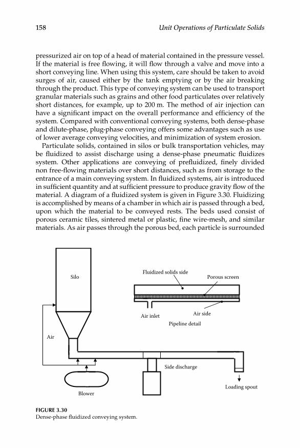
158 Unit Operations of Particulate Solids
pressurized air on top of a head of material contained in the pressure vessel. If the material is free flowing, it will flow through a valve and move into a short conveying line. When using this system, care should be taken to avoid surges of air, caused either by the tank emptying or by the air breaking through the product. This type of conveying system can be used to transport granular materials such as grains and other food particulates over relatively short distances, for example, up to 200 m. The method of air injection can have a significant impact on the overall performance and efficiency of the system. Compared with conventional conveying systems, both dense-phase and dilute-phase, plug-phase conveying offers some advantages such as use of lower average conveying velocities, and minimization of system erosion.
Particulate solids, contained in silos or bulk transportation vehicles, may be fluidized to assist discharge using a dense-phase pneumatic fluidizes system. Other applications are conveying of prefluidized, finely divided non free-flowing materials over short distances, such as from storage to the entrance of a main conveying system. In fluidized systems, air is introduced in sufficient quantity and at sufficient pressure to produce gravity flow of the material. A diagram of a fluidized system is given in Figure 3.30. Fluidizing is accomplished by means of a chamber in which air is passed through a bed, upon which the material to be conveyed rests. The beds used consist of porous ceramic tiles, sintered metal or plastic, fine wire-mesh, and similar materials. As air passes through the porous bed, each particle is surrounded
Air inlet
Air
Side discharge
Loading spoutBlower
Silo
Air side
Fluidized solids sidePorous screen
Pipeline detail
Figure 3.30Dense-phase fluidized conveying system.

Storage and Conveying of Bulk Solids 159
by a film of air. At the point of incipient fluidization, the material starts behaving as a free-flow powder or particulate. Fluidized solids may be forced through pipelines by air under pressure passed through a perforated flexible inner tube running the length of the pipeline. The fluidized material is then conveyed by establishing a pressure drop along the pipeline. Fluidized sys-tems are the most reliable and economical method of conveying certain pow-ders and bulk solids over distances ranging from few meters up to about 1 km. They take advantage of the fluidization and air-retention properties of the bulk solid (Mainwaring and Reed, 1987). The suitability of a given mate-rial to this mode of conveying, and the best type of feeder for these systems should be determined by test work.
A blow tank is a type of slow-motion, dense-phase pneumatic conveying that allows friable products to be conveyed with extremely low levels of product degradation or damage, because solids conveying velocities usually occur in the range of 0.25–2 m/s. Such features are very important for a wide variety of friable products, especially for those prone to attrition. Low-velocity systems operate at relatively high conveying pressures, for example, 200–500 kPa, and consequently must have reliable hardware. Also, due to the extremely high levels of concentration which occur during conveying, the subsequent operation conditions depend quite strongly on the nature and physical properties of the material being transported. It is important, for these reasons, that full-scale tests be exercised prior to the selection or design of such equipment.
One of the most interesting and innovative applications of dense-phase pneumatic conveying is the long-distance transportation. Conveying of fine and coarse materials over distances up to 3 or 4 km is possible with this sys-tem. This can be achieved by tandem arrangement of blow tanks. Long-distance systems operate at high pressures and particular attention must be given to the control of solids feeding into the pipeline. A manner of doing this is by using a cone-dosing system, in which the flow of solids is con-trolled by the movement of a double cone located near the blow tank outlet. The cone moves continuously up and down inside the vessel, but the stroke is adjusted by a proportional-integral controller, based on a conveying line back-pressure measuring signal and set point. The higher the conveying or operating pressure, the lower the cone set point inside the vessel. The flow of solids into the conveying pipeline is restricted on this manner, until a satis-factory conveying pressure is restored. Furthermore, the cone dosing system provides an additional and useful feature of mechanical agitation, as well as flow assistance of cohesive materials.
3.5.5.3 Dilute-Phase Systems
As stated earlier, dilute-phase conveying is the commonly employed method for transporting a wide variety of suspended solids using air flowing axially along a pipeline. The method is mainly characterized by the low solids to air
160 Unit Operations of Particulate Solids
ratio and by the fact that air and solids flow as a two-phase system inside a pipeline. The main components of dense-phase pneumatic conveying sys-tems basically include gas movers, solids feeders, pipelines, and solids sepa-rators. Their location within the system may vary from type to type but their functions are the same. The gas mover provides an appropriate flow rate of gas required for the transport at the right velocity and pressure. The solids feeder introduces the solids particles at a controlled rate into the pipeline where they are mixed with the conveying gas. The pipeline consists of straight sections, both horizontal and vertical, connected together with bends. At the end of the trajectory, in any type of solid–gas separator, the solids are decelerated and recovered from the gas stream to be stored in a silo or fed into another unit. The gas, which is typically air, is generally released into the atmosphere. Secondary components comprise controls, safety equipment, and instrumentation.
By far, the most common device for moving gas in a pneumatic conveying system is the Roots-type, rotary lobe blower. Such blower is preferred since it provides an economical source of gas flow that meets the pressure or vac-uum and flow requirements for the largest category of systems. An impor-tant feature of this type of blower is that it delivers a nearly constant volume over its operating pressure range. This is important because control of the gas in pneumatic conveying system is critical for stable operation. Single-stage blowers generate up to 200 kPa while double-stage blowers generate up to about 270 kPa. For low-pressure conveyors, centrifugal fans can be used as gas movers. High-speed, single-stage centrifugal fans deliver air at about 120 kPa and must be supplied with clean air if excessive abrasion of the light impellers is to be avoided. The slower-running, multistage, heavy-duty cen-trifugal fan can deliver up to 140 kPa and, being slower running, is relatively resistant to particle abrasion. Compressors deliver air at high pressures but require lubrication being, thus, potential contaminants of the solids in move-ment. They provide pressures up to 800 kPa so, with certain measures, they find applications in high-pressure systems, as well as in dense-phase conveying.
For proper operation of a dilute-phase, pneumatic conveying system the solids fed into the pipeline must be carefully controlled. Two common types of feeders are the venturi feeder and the rotary valve or star feeder, illus-trated in Figure 3.31. The venturi feeder is only suitable for low-pressure systems. The rotary valve feeder, also known as star feeder as described previously in this chapter is widely used for feeding medium-pressure conveyors. This feeder is efficient and simple in principle, but requires care-ful design in order to minimize air leakage. Excessive air loss from feeders, wastes power, causes dust, and leads to system instability. Rotary feeders work well on free-flowing, nonabrasive powders and special types are available for more difficult materials.
The number and type of bends used in the pipeline may constitute a criti-cal design problem. The difficulties that may arise by the use of bends are

Storage and Conveying of Bulk Solids 161
abrasive wear, product degradation, product buildup, and pressure loss. The latter is the problem primarily related to operation. In general terms, all the bend associated drawbacks are minimized by use of smooth, long-radius bends instead of short radius and blind tees types of bends. The system lay-out is also important. It is often more troublesome to have many bends in short distances than few bends in long distances. In the former case, the con-tribution of each bend will be more significant than in the latter. However, for systems handling nonabrasive, nondegradable materials, the number and type of elbow is not very critical and selection or design should probably be based on cost.
Separating the solids from the airstream when conveying concludes can be accomplished in a number of ways. For most of the cases, a single technique is insufficient to separate the conveyed material completely and satisfactory. The most common approach consists in using a cyclone followed by a bag filter. Both separating techniques will be discussed in a later chapter. The selection of a gas–solids separating system should be based on the material characteristics, degree of separation required, environmental regulations, concentration of solids, and cost.
Operating variables of dilute-phase conveying systems comprise gas (air) velocity, pressure drop, gas-solids ratio, and particle properties. Pertaining air velocity, most particulate materials may be conveyed satisfactorily at air speeds within the range of 15–25 m/s. Velocities above this may cause abra-sion of tube bends and product damage may represent difficulties. At extremely low speeds, solids tend to settle out and block horizontal pipe runs. In terms of pressure drop, if air at high pressure is used, its corre-spondingly high initial energy will enable more conveying to be accom-plished, per kilogram of air, than if low-pressure air is used. High-pressure systems are, however, proportionately more expensive than low-pressure ones. The maximum pressure recommended for general-purpose, dilute-phase conveying of solid particulate materials is about 170 kPa. With regard to solid–air ratio, for maximum efficiency this should be as high as possible, but without invading the range of dense-phase conveying. There is an upper
Air
Sliding gate
(a) (b)
Sliding gate
Air
Figure 3.31Feeders for dilute-phase conveying systems: (a) venture feeder and (b) star feeder.

162 Unit Operations of Particulate Solids
limit for this ratio for specific materials; exceeding it will cause blockage of the system due to saltation. Finally, material properties such as size, shape, density, and surface properties need to be carefully considered in operation and selection of dilute-phase conveying systems. Other important properties are friability, hygroscopicity, as well as susceptibility to impact, abrasion damage or oxidation.
Figure 3.32 shows the four main types of dilute-phase conveying systems previously mentioned. The pressure system, also called positive-pressure, or push system operates at super-atmospheric pressure and is used for delivery to several outlets from one inlet (Figure 3.32a). Although most applications of these systems lie within the scope of dilute-phase conveying, under certain arrangements they can also operate as high-pressure, dense-phase
Separators
Silos
Blower
Airfilter
(a)
(c)
(b)
(d)
Separator
Silo
Blower
Slidegates
Silos
Silo
Separators
Blower
Airfilter
Slide gates
Silos
Silos
Separators
Blower
Airfilter
Feed
Feed
Figure 3.32Dilute-phase pneumatic conveying systems: (a) pressure system, (b) vacuum system, (c) combined system, and (d) closed-loop system.

Storage and Conveying of Bulk Solids 163
conveyors. In general, pressure systems can hold higher capacities and longer conveying distances than negative-pressure systems. The vacuum, negative-pressure or pull system, works at subatmospheric pressure and is used for delivery to one outlet from several inlets (Figure 3.32b). Vacuum systems are usually limited to shorter distances than positive ones and are more restrained to operate with dilute, low solids loading than pressure systems. When both features of pressure and vacuum systems are combined in a unit, the advantages of each can be exploited (Figure 3.32c). This arrangement con-sists of two sections: a pull/push system with a negative-pressure front end, followed by a positive-pressure loop. The benefit is that they capitalize on the ease of feeding into a vacuum and combine this with the higher capacity and longer conveying distance when using positive pressure. Recirculation of the conveying air, as in the closed-loop system (Figure 3.32), reduces contamina-tion of product by the air and limits product dehydration. However, such systems are often difficult to control and an intercooler may be required to prevent the pump overheating the recirculated air.
3.5.5.4 Design and Selection of Dilute-Phase Systems
In contrast with those conveying methods previously discussed, pneumatic conveying can be perfectly identified as a case of two-phase flow, which is a topic well covered by fluid mechanics. Single-phase flow within a pipe can be described by basic equations that are considered the basic fundamentals to start calculations in order to design pneumatic conveying systems. However, while single-phase flow in a pipe is well understood, adding solids into the moving stream in the so-called two-phase flow complicates matters significantly. As solid particles are introduced in a moving stream of gas, the pressure drop in the line begins to increase because momentum is trans-ferred to the particles to accelerate them to the conveying velocity. The total pressure drop consists of two components: the one due to the gas flow alone, and that required for transporting the particles. Apart from the gas velocity, some other variables such as the amount of solids in the pipeline and the velocity of the solids relative to the gas also affect the pressure drop.
The moving gas stream applies drag and lift to the particles. For particles to be conveyed in such gas stream, the velocity of the gas must be sufficiently high to stop particles settling out. In flow through horizontal pipes the mini-mum air velocity to stop particles settling to the bottom of the pipe is called the saltation velocity. The equivalent velocity for flow through vertical pipes is known as the choking velocity. The saltation velocity is a function of the density of the gas and the solids, as well as particle and pipeline diameter (Cabrejos and Klinzing, 1994). There is also a direct relationship between the saltation velocity and the solids loading ratio. Generally, saltation occurs at higher velocities when the solids loading ratio is also high.
In terms of designing equipment for pneumatic conveying, there is another type of velocity, that is, the minimum conveying velocity, used to describe

164 Unit Operations of Particulate Solids
the correlation of gas velocity to the behavior of solid particles inside a pipe-line. This velocity is the lowest one necessary to prevent plugging the line in a given system for a given material. Some researchers have suggested the use of the saltation velocity with a safety factor, while others have developed empirical correlations. Some of these correlations, however, often predict widely differing velocities for the same set of conditions (Wypych, 1999).
The saltation velocity can be calculated based on the procedure presented by Zenz (1964), as follows:
Calculate the parameter xp∗ by the equation:
xx
gp
p
g g s g
∗ =− 3 2
1 3( ) ( )
/µ ρ ρ ρ4
(3.27)
where xp is the particle diameter, μg is the gas viscosity, ρg and ρs are the gas and solid densities, respectively. If there is a mixture of particle sizes, that is, a particle size distribution which is quite common in most industrial powders, calculate xp
∗ for the largest and smallest particle.From Figure 3.33 calculate uss
∗ from xp∗ and use the following relation to
determine the minimum conveying velocity uss for a single particle:
u u
gDss ss
g s g
gt=
−
∗0 19
43 2
1 3
0 4. ( )( )( )
( )/
.µ ρ ρ
ρ
(3.28)
where Dt is the pipe diameter in mm, but taken as dimensionless in the above equation.
Estimate n, the gradient of the curve in Figure 3.33 at xp∗ . For a particle size
distribution n is the slope of the line joining the values of uss∗ for the largest
and smallest particle.
10
Para
met
er (u
* ss)
1 10 100 10001
100
Parameter related to particle size (x*p)
Figure 3.33Minimum conveying velocity for a single particle for a pipe diameter Dt of 63.5 mm. (Adapted from Zenz, F. A. 1964. Industrial and Engineering Chemistry Fundamentals 3: 65–75.)

Storage and Conveying of Bulk Solids 165
Transpose us , the saltation velocity from the following equations:
G n u uu
s
s
s ss
ssρ =−0 214 1 5. ( ) ( ).
(3.29)
for n > 0.068, or
G u uu
s
s
s ss
ssρ =−0 003. ( )2
(3.30)
for −0.11 < n < 0.068.In Equations 3.28 and 3.29, Gs is the flux of solids. For particle size distribu-
tions, the largest particle size should be used in these equations in order to avoid underestimation of the saltation velocity.
Pressure drop is another key variable involved in design and operation of pneumatic conveying systems. Pressure drop requirement is closely associ-ated with gas flow and solids rate. The same amount of solids can be con-veyed in a line using a number of velocity and pressure drop combinations. Pressure drop in pneumatic conveying is determined by calculating poten-tial energy, kinetic energy, and frictional energy changes in horizontal and vertical sections, as well as in bends in the conveying line separately. The estimation of the overall pressure drop results from summing up all the individual contributions, depending on the specific layout of a pneumatic conveying system. The detailed procedure is as follows:
Take the initial air velocity as 10% above the saltation velocity, to minimize risk of settling of coarse particles.
In horizontal sections the potential energy loss is zero, the kinetic energy gain Ek is given by
E G uk s p= (3.31)
where Gs is the flux of solids and up is the particle velocity.If particle has accelerated to its maximum value, the particle velocity is
defined by
u u up t= −0 (3.32)
where u0 is the air velocity and ut is the terminal settling velocity of the particle.
The behavior of particles settling in a fluid is well understood, and the set-tling velocity depends on the flow regime, that is,
u
x gt
p s g
g=
−2
18( )ρ ρ
µ (3.33)

166 Unit Operations of Particulate Solids
for Rep < 0.4, which is the well-known Stokes’ law. Also:
u
gxt
s g
g gp=
−
4225
2 2 1 3( )
( )/ρ ρ
ρ µ
(3.34)
for Rep < 500. And, finally:
u
x gt
p s g
g=
−
3 1 1 2. ( ) /ρ ρρ
(3.35)
for Rep < 2 × 10⁵.In Equations 3.32 through 3.34, Rep refers to the particle Reynolds number,
which is defined by
Rep
p g t
g=
x uρµ
(3.36)
and all the variables have been previously defined.The frictional energy loss due to the gas flow Efg is given by
E
f u LDfg
g g=2 0
2ρ
(3.37)
where fg is a gas friction factor, L is the pipe length, and D is the pipe diam-eter. The gas friction factor fg, adopts values according to the system Reynolds number Re, that is,
fg = −0 0791 0 25. (Re) .
(3.38)
for 3 × 10³ < Re < 105. And
fg = + −0 0008 0 0552 0 237. . (Re) .
(3.39)
for 105 < Re < 108.As indicated above, the Reynolds number in Equations 3.37 and 3.38 is that
for the system, that is,
Re =
D uρµ
g
g
0
(3.40)
The frictional energy loss due to the particle flow Efp can be estimated by
E
ff
GG
Efpp
g
s
g
sfg8
=
π ρρ
1 2/
(3.41)

Storage and Conveying of Bulk Solids 167
where G is the flux of air and fp is the particle friction factor, which can be determined graphically, as a function of Re, from Figure 3.34.
The frictional loss in flow round bends Efb can be calculated from:
E f
GG
uufb b
s
pg=
2 0
3
ρ
(3.42)
where fb equals 0.375, 0.188, or 0.125 for bend radius: pipe diameter ratios of 2, 4, or 6 or more, respectively.
For vertical sections, there will be normally no kinetic energy change. The frictional energy losses are calculated as for the horizontal sections. The potential energy gain Ep is given by
E
GG
uu
ghps
ps=
0 ρ
(3.43)
where h is the height of the section.As stated earlier, the sum of all the energy losses described above, apply-
ing for a particular system layout, will give the total pressure drop through the conveyor. A practical approach for preliminary calculations in selection and design of pneumatic conveying systems is the use of nomographs, such as those presented by Green and Perry (2008).
example 3.6
Calculate the power required to convey pneumatically 1500 kg/h of a flour of 1300 kg/m3 density, with the particle size distribution given in Table 3.11. The
0.0003
0.0002
0.0001
0.00007
1 2 3 5 8 ×10⁴
System reynolds number (Re)
Part
icle
fric
tion
fact
or (
f p)
Figure 3.34Particle friction factor as a function of system Reynolds number, Re. (Adapted from Rose, H. E. and Barnacle, H. F. 1957. Engineer, London 203: 898, 939.)
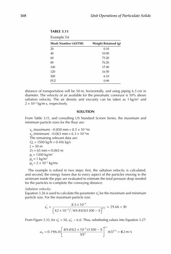
168 Unit Operations of Particulate Solids
distance of transportation will be 50 m, horizontally, and using piping 6.5 cm in diameter. The velocity of air available for the pneumatic conveyor is 10% above saltation velocity. The air density and viscosity can be taken as 1 kg/m3 and 2 × 10⁻⁵ kg/m s, respectively.
SoluTion
From Table 3.11, and consulting US Standard Screen Series, the maximum and minimum particle sizes for the flour are:
xp (maximum) ~0.850 mm = 8.5 × 10⁻⁴mxp (minimum) ~0.063 mm = 6.3 × 10⁻⁵mThe remaining relevant data are:Qs = 1500 kg/h = 0.416 kg/sL = 50 mDt = 65 mm = 0.065 mρs = 1300 kg/m3
ρg = 1 kg/m3
μg = 2 × 10⁻⁵ kg/ms
The example is solved in two steps: first, the saltation velocity is calculated, and second, the energy losses due to every aspect of the particles moving in the airstream inside the pipe are evaluated to estimate the total pressure drop needed for the particles to complete the conveying distance.
Saltation velocity:Equation 3.26 is used to calculate the parameter xp
∗ for the maximum and minimum particle size. For the maximum particle size:
xp*
/
.
( ) ( . )( )( ).= ×
× − = ≈
−
−
8 5 10
3 2 10 4 9 81 1 1300 129 66 0
4
5 2 1 3 3
From Figure 3.33, for xp∗ = 30, uss 6.0.∗ ~~ Thus, substituting values into Equation 3.27:
uss = × −
≈
−
0 19 6 04 9 81 2 10 1300 1
3165
5
2
1 3
0 4. ( . )( . )( )( )
( )( )
/
. 44 2 m s. /
Table 3.11
Example 3.6
Mesh Number (ASTM) Weight Retained (g)
20 0.1040 10.0060 73.2080 76.20100 17.00120 16.50200 6.10PLT 0.90

Storage and Conveying of Bulk Solids 169
To evaluate the slope in Figure 3.33, and continue solving the example, the value of xp
∗ minimum is needed, and it is calculated following the same procedure as above. Using, thus, Equation 3.26, a value of xp
∗ for the minimum particle size (6.3 × 10⁻⁵ m) of about 2.2 is obtained.
Using the plot in Figure 3.33 the values y2 and y1 corresponding to values x2 = 30 and x1 = 2 are, approximately, 6 and 4, so the slope of the line joining the points for the maximum and minimum particle sizes is
n = −
−≈6 4
30 20 0. 7
The slope n is, therefore, greater than 0.068, so that Equation 3.28 should be used to substitute values, as follows:
125 361300
0 214 0 07 4 24 2
1 5. . ( . ) ( . ).
.
= −us
where the flux of solids Gs is calculated from the relationship between the mass flow rate and the cross-sectional area of the pipe, that is:
G
QA
s2kg/s
mkg/m s= = =0 416
0 0033125 362
.
..
Transposing for us, the saltation velocity is
us = 106.4 m/s
Adding 10% to the saltation velocity, the initial air velocity in the pneumatic conveying is calculated as
u0 ≈ 117 m/s
The kinetic energy of the particles is defined by Equation 3.30, where the par-ticle velocity up is a function of the terminal settling velocity ut, depending itself on the settling regime, as explained in Section 3.5.5.4. Iterations are, therefore, needed. Assuming applicability of Equation 3.32 to calculate ut, it is found that the value of the particle Reynolds number Rep surpasses the limit of 0.4, so a second approach using Equation 3.33 is done, that is,
ut = −
×
× ≈−
−4 1300 1 9 812251 2 10
8 5 10 4 462 2
5
1 3
4( ) ( . )( )( )
( . ) ./
mm/s
verifying the applicability using Rep:
Re
( . )( . )( ).p = ×
×=
−
−8 5 10 4 46 1
2 10189 5
4
5

170 Unit Operations of Particulate Solids
agreement is found with the limiting values of Rep between 0.4 and 500, so the particle velocity is: up = 117 − 4.46 = 112.54, and the particle kinetic energy is
Ek214,1 8 N m= ≈( . )( . ) /125 36 112 54 0
The frictional energy lost due to the gas flow is determined by Equation 3.36, where the value of the friction factor fg depends on the system Reynolds number, that is,
Re
( . )( )( ),=
×=−
0 065 117 12 10
0 05 38 25
using, therefore, Equation 3.38:
fg 33 43 1= + ≈ ×− −0 0008 0 0552 380250 00 237. . ( ) ..
and the frictional energy lost due to the gas flow from Equation 3.36 is:
Efg
272,173N m= × ≈−2 3 43 10 1 117 50
0 065
3 2( . )( )( ) ( ).
/
The frictional energy lost due to the particle flow can be estimated using Equation 3.40. In such equation, the gas flux may be calculated as the product of the gas velocity by its density. Since the air density equals unity, the gas flux is: G = 117 kg/m2 s. Also, the particle friction factor fp to be substituted into Equation 3.40 can be determined from the system Reynolds number Re as in Figure 3.34. In such figure, for Re = 380,250, fp = 0.00007. Substituting, thus, all the values in Equation 3.40:
Efp =
π8
0 000070 00343
13001
125 36117
2..
. ≈( ) /72173 22365 N m2
The total pressure drop is the sum of all the above energy losses, that is,
∆P 1 9 kN mtotal k fg fp2= + + = + + = ≈E E E 14108 72173 22365 108646 0 /
The power can be calculated as the product of the volumetric flow rate of air and the total pressure drop. The volumetric flow rate of air Qair is the product of the air velocity and the cross-sectional area of the conveying pipe, that is, Qair = (117)(0.0033) = 0.3861 m3/s. The power would, therefore, be
(ΔPtotal)(Qair) = (108646N/m2)(0.3861m3/s) = 41948.22 ≈ 42000 WFinally, the horsepower can be determined as
Power = =41984 22735 4996
0.
..
Whp/W
57 8 hp

Storage and Conveying of Bulk Solids 171
3.6 Laboratory Exercise: Pneumatic Conveying Characteristics of Different Granules
3.6.1 introduction
Pneumatic conveying can be defined as the transport of solid materials, from one place to another, using a transporting gas. The materials can be moved through the pipe with air, but sometimes nitrogen is used for materials that could cause a chemical reaction with the air. One of the most important issues in pneumatic conveying is how to transport the materials with the lowest pressure drop and thus least amount of energy. The pressure drop behavior can be observed by preparing a state diagram. A state diagram is a plot of pressure difference versus the transport gas velocity at a fixed solid flow rate. The objective of the experiment is to derive a basic phase diagram using, at least, two different testing materials.
3.6.2 equipment and Materials
A laboratory or pilot-scale conveying system comprising: hoppers, air com-pressor, rotary feeder, polyvinyl chloride (PVC) conveying pipe, control valves, pressure transducers, rotameter, and electronic weight indicator. Polypropylene granules of different size, as testing material.
3.6.3 Procedure
Operate the compressor to introduce air into the conveying pipe •connected to the feed hopper by means of the rotary feeder, by open-ing the air control valve.Drive granules into the conveying line by the feed hopper using the •rotary feeder. Handle the valves in order to control solids and air flow rate.Control the air flow rate via the rotameter located after the air valve •controlling the airstream from the compressor and before the rotary feeder.Allow the granules to get into a recycle solids hopper, feed an inter-•mediate hopper by closing the valve after the recycle solids hopper to enable the mass solids flow rate to be measured using the elec-tronic weight indicator adapted to the intermediate hopper.Carry out two to three runs varying the solids fed, and the air and •solids flow rate by handling the control valves.Take readings of the air velocity, pressure at the different pressure •transducers, and the weight of solids passing through the intermedi-ate hopper.

172 Unit Operations of Particulate Solids
3.6.4 Calculations and report
Tabulate data on air superficial velocity, solids mass flux, and aver-•age pressure gradient between pressure transducers points, for all the experimental runs.Derive a plot of superficial air velocity for different values of solids •mass flux versus the pressure gradient, for the different granular solids studied. This plot represents the phase diagram for the con-veying process.Present a complete written report, according to scientific report •guidelines, either given by instructor or consulted in the literature. Include graphs, charts, and calculations carried out, as well as dis-cussion on own data. Compare results, also, with data from a litera-ture search and present a written report, including a thoughtful discussion on the comparative aspects mentioned.
PROBLEMS
1. A silo is to be designed to store granular material of 480 kg/m3 in bulk density. The material is kept on the open forming conical heaps 7.5 m long and 2 m high. A metal cylinder, 2.5 m diameter and 10 m long, may be adapted to construct the silo. The maxi-mum pressure on the base of the cylinder is 14 kPa and the friction coefficient μ’ for the granular material is 0.5. Suggest, supported by calculations, whether the cylinder could be adapted to build a silo to store the granular material.
2. Predict the basic dimensions of a silo to store 32 tons of a par-ticulate solid of 1600 kg/m3 density. The material has uniformly sized particulates of 1 mm. The angle of repose of the material is 32° while its friction coefficient μ’ is 0.48. The maximum pressure allowed at the bottom of the cylindrical part of the silo is 3.5 kPa.
3. Suggest the optimum outlet dimension of a conical hopper in a silo storing moist crushed limestone of 1350 kg/m3 density. The results of characterizing the limestone using in terms of failure properties are presented in Tables 3.12 through 3.14.
4. Calculate the saltation velocity for transporting grains with a lim-iting size of 2 mm and a density of 1300 kg/m3, through a pipe of 6.5 cm in diameter. Air density can be taken as 1 kg/m3 and air viscosity as 2 × 10⁻⁵ kg/m s.
Table 3.12
Wall Friction Angle of Crushed Limestone for Three Moisture Contents (Table for Problem 3)
2.5% 3.8% 5.0%
29° 28° 28.5°
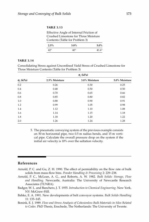
Storage and Conveying of Bulk Solids 173
5. The pneumatic conveying system of the previous example consists on 50 m horizontal pipe, two 0.5 m radius bends, and 15 m verti-cal pipe. Calculate the overall pressure drop on the system if the initial air velocity is 10% over the saltation velocity.
References
Arnold, P. C. and Gu, Z. H. 1990. The effect of permiability on the flow rate of bulk solids from mass-flow bins. Powder Handling & Processing 2: 229–238.
Arnold, P. C., McLean, A. G., and Roberts, A. W. 1982. Bulk Solids: Storage, Flow and Handling. Newcastle, Australia: The University of Newcastle Research Associates (TUNRA).
Badger, W. L. and Banchero, J. T. 1955. Introduction to Chemical Engineering. New York, NY: McGraw-Hill.
Bahke, E. A. 1991. New developments of belt conveyor systems. Bulk Solids Handling 11: 135–145.
Benink, E. J. 1989. Flow and Stress Analysis of Cohesionless Bulk Materials in Silos Related to Codes. PhD Thesis, Enschede, The Netherlands: The University of Twente.
Table 3.14
Consolidating Stress against Unconfined Yield Stress of Crushed Limestone for Three Moisture Contents (Table for Problem 3)
σ1 (kPa)
σc (kPa)
2.5% Moisture 3.8% Moisture 5.0% Moisture
0.2 0.26 0.30 0.250.4 0.48 0.50 0.500.6 0.70 0.65 0.660.8 0.85 0.80 0.821.0 0.88 0.90 0.911.2 0.99 1.05 0.981.4 1.12 1.10 1.081.6 1.14 1.15 1.181.8 1.18 1.20 1.222.0 1.26 1.24 1.28
Table 3.13
Effective Angle of Internal Friction of Crushed Limestone for Three Moisture Contents (Table for Problem 3)
2.5% 3.8% 5.0%
42° 40° 41.6°

174 Unit Operations of Particulate Solids
Cabrejos, F. J. and Klinzing, G. E. 1994. Minimum conveying velocity in horizontal pneumatic transport and the pickup and saltation mechanisms of solid parti-cles. Bulk Solids Handling 14: 541–550.
Carson, J. W., Royal, T. A., and Goodwill, D. J. 1986. Understanding and eliminating particle segregation problems. Bulk Solids Handling 6: 139–144.
Clague, K. 1973. The Effects of Stresses in Bunkers. PhD Thesis. Nottingham: University of Nottingham.
Colijn, H. and Peschl, A. S. Z. 1981. Non-symmetrical bin flow problems. Bulk Solids Handling 1: 377–384.
Foote, B. L., Bobbie, L., Radidran, A., and Badiru, A. B. 1988. Simulation and network analysis payoff in conveyor system analysis. Industrial Engineering 20: 48–53.
Green, D. W. and Perry, R. H. 2008. Perry’s Chemical Engineers’ Handbook, 8th Ed. New York, NY: McGraw-Hill.
Häußler, U. and Eibl, J. 1984. Numerical investigations of discharging silos. Journal of Engineering Mechanics 110: 957–971.
Janssen, H. A. 1895. Versuche über getreidedruck in silozellen. Zeitschrift des Vereins Deutscher Ingenieure 39: 1045–1049.
Jenike, A. W. 1964. Storage and Flow of Solids. Bulletin No. 123 of the Utah Engineer Experiment Station. Salt Lake City UT: University of Utah.
Jenike, A. W. and Johanson, J. R. 1968. Bin loads. Journal of Structural Division, ASCE 95: 1011–1015.
Jenike, A. W. and Johanson, J. R. 1969. On the theory of bin loads. Journal of Engineering for Industry, Transactions of the ASME Series B 91: 339–342.
Johanson, J. R. 1965. Method of calculating rate of discharge from hoppers and bins. AIME Transactions 232: 69–80.
Johanson, J. R. 1982. Controlling flow patterns in bins by the use of an insert. Bulk Solids Handling 2: 495–498.
Mahmound, M. H. 1977. Practical finite element modeling of silo-material interaction. Proceedings of the Technical Program, International Powder and Bulk Solids Handling & Processing Conference, Rosemont, IL, USA.
Mainwaring, N. J. and Reed, A. R. 1987. Permeability and air retention characteristics of bulk solid materials in relation to modes of dense-phase pneumatic conveyor performance. Bulk Solids Handling 7: 415–425.
Manjunath, K. S. and Roberts, A. W. 1986. Wall pressure-feeder load interactions in mass-flow hopper/feeder combinations: Part I. Bulk Solids Handling 6: 769–775.
Manjunath, K. S. and Roberts, A. W. 1986b. Wall pressure-feeder load interactions in mass-flow hopper/feeder combinations: Part II. Bulk Solids Handling 6: 903–911.
Marinelli, J. and Carson, J. W. 1992. Solve solids flow problems in bins, hoppers and feeders. Chemical Engineering Progress 88: 22–28.
McLean, A. G. 1979. Flow Rates of Simple Bulk Solids from Mass-Flow Bins. PhD Thesis. Wollongong, Australia: University of Wollongong.
McLean, A. G. 1990. Improved stockpile performance. Bulk Solids Handling 10: 19–22.Merrow, E. W. 1988. Estimating startup times for solids-processing plants. Chemical
Engineering 89: 89–92.Mitman, E. T. 1991. Dome silo storage systems. Bulk Solids Handling 11: 71–72.Reed, A. R. and Bradley, M. S. A. 1991. Advances in the design of pneumatic convey-
ing systems. A United Kingdom perspective. Bulk Solids Handling 11: 93–97.

Storage and Conveying of Bulk Solids 175
Roberts, A. W. 1988. Modern Concepts in the Design and Engineering of Bulk Solids Handling Systems. Newcastle, Australia: The University of Newcastle Research Associates (TUNRA).
Roberts, A. W. 1988b. Some aspects of grain silo wall pressure research-influence of moisture content on loads generated and control of pressures in tall multi-outlet silos. Proceedings of the 13th International Powder and Bulk Solids Conference, Chicago.
Roberts, A. W. 1994. Advances in the design of mechanical conveyors. Bulk Solids Handling 14: 255–281.
Roberts, A. W. 1999. The influence of granular vortex motion in the volumetric per-formance of enclosed screw conveyors. Powder Technology 104: 56–67.
Roberts, A. W. 2000. Predicting the performance of enclosed screw conveyors. From Powder to Bulk Conference. IMechE, London, June 2000.
Roberts, A. W. and Teo, L. H. 1990. Design considerations for maximum reclaim capacity of conical stockpiles. Bulk Solids Handling 10: 9–15.
Roberts, A. W., Ooms, M., and Scott, O. J. 1986. Influence of vibrations on the strength and boundary friction characteristics of bulk solids and the effect on bin design. Bulk Solids Handling 6: 161–169.
Roberts, A. W., Ooms, M., and Wiche, S. J. 1990. Concepts of boundary friction, adhe-sion and wear in bulk solids handling operations. Bulk Solids Handling 10: 189–198.
Rose, H. E. and Barnacle, H. E. 1957. Flow of suspensions of non-cohesive spherical particles in pipes. Engineer, London 203: 898, 939.
Royal, T. A. and Carson, J. W. 1993. How to avoid flooding in powder handling sys-tems. Powder Handling & Processing 5: 63–67.
South, D. B. 1991. Curved bin walls. Bulk Solids Handling 11: 75–76.Terziovski, M. and Arnold, P. C. 1990. On the effective sizing and placement of air
blasters. Bulk Solids Handling 10: 181–185.Thomson, F. M. 1997. Storage and flow of particulate solids. In: Handbook of Powder
Science and Technology, Fayed, M. E. and Otten, L. (eds.). New York, NY: Chapman & Hall.
Walker, D. M. 1966. An approximate theory for pressure and arching in hoppers. Chemical Engineering Science 21: 975–978.
Walker, K. 1990. Pendular bucket wheel stacker reclaimer system. Bulk Solids Handling 10: 25–26.
Walters, J. K. 1973. A theoretical analysis of stresses in silos with vertical walls. Chemical Engineering Science 28: 13–15.
Wohlbier, R. H. 1977. Stacking, Blending & Reclaiming of Bulk Materials. Zurich: Trans Tech Publications.
Wypych, P. W. 1999. The ins and outs of pneumatic conveying. International Symposium on Reliable Flow of Particulate Solids III. Porsgrunn, Norway, August 11–13, 1999.
Zenz, F. A. 1964. Conveyability of materials of mixed particle size. Industrial and Engineering Chemistry Fundamentals 3: 65–75.

Part II
Bulk Solids Processing


179
4Size Reduction
4.1 Fundamental Principles of Comminution
4.1.1 introductory aspects
In many applications of the material processing industry, frequently size reduction of solid materials for different purposes is necessary. For example, size reduction may be a specific requirement of a process or may aid other operations such as expression or extraction. Comminution is the generic term used for size reduction, although such a term includes operations such as crushing or pulverizing. The reduction mechanism consists of deforming the solid piece until it breaks or tears. Breaking of hard materials along cracks or defects in their structures is accomplished by applying diverse forces.
The objective of comminution is to produce small particles from larger ones. Smaller particles are the desired product either because of their large surface or because of their shape, size, and number. The energy efficiency of the operation can be related to the new surface formed by the reduction in size. The geometric characteristics of particles, both alone and in mix-tures, are important in evaluating a product from comminution. In an actual process, a given unit does not yield a uniform product, whether the feed is uniformly sized or not. The product normally consists of a mixture of particles, which may contain a wide variety of sizes and even shapes. In comminuted products, the term “diameter” is generally used to describe a characteristic dimension related to particle size. As described in Chapter 2, the shape of an individual particle is conveniently expressed in terms of the sphericity Φs, which is independent of particle size. For spherical particles, Φs equals unity, while for many crushed materials, its value lies between 0.6 and 0.7.
The different types of particle size distributions have been discussed extensively in Chapter 2. No single distribution applies equally well to all comminuted products, particularly in the range of coarser particle sizes. For finer particles, however, the most commonly found distribution follows a log-normal function (Herdan, 1960), which is the most useful one among the different types of functions (Beddow and Meloy, 1980).

180 Unit Operations of Particulate Solids
4.1.2 Forces involved in Size reduction
As previously mentioned, in comminution of solid materials, the reduction mechanism consists of deforming the solid piece until it breaks or tears and such breaking may be achieved by applying diverse forces. The types of forces commonly used in processing industries are compressive, impact, attrition or shear, and cutting. In a comminution operation, more than one type of force acts, usually. Compressive forces are used for coarse crushing of hard materials. Coarse crushing implies reduction to a size of about 3 mm. Impact forces can be regarded as general purpose forces and may be associ-ated with coarse, medium, and fine grinding of a variety of materials. Shear or attrition forces are applied in fine pulverization, when size of products can reach the micrometer range. Sometimes a term referred as ultrafine grinding is associated with processes in which the submicron range of particles is attained. Finally, cutting gives a definite particle size and may even produce a definite shape.
A good number of industrial powders have been produced by crushing of large size pieces. For example, metallic and nonmetallic minerals are extracted from the earth crust in the form of rocks and boulders, but in their final presentation, in products such as carbonates, limestone, or silicates, their appearance is that of fine powders containing particles whose equiva-lent diameters could well be in the order of micron fractions. It is not possible to reduce the size of a solid material in a single operation and with a single equipment from its macroscopic range of size (e.g., rocks) to its final form of fine powder. The processes of size reduction are carried out, consequently, in stages or defined ranges of reduction. Regularly, the size reduction within the limits of the macroscopic range of objects is named coarse reduction, which applied in the mesoscopic range is known as intermediate reduction, while the one corresponding to the microscopic range is defined as fine reduction. The kinds of forces commonly used in size reduction operations correspond, usually, to such specificity of ranges. Thus, predominating forces in coarse reduction are compressive forces, in intermediate reduction are impact forces, and in fine reduction are shearing forces. Table 4.1 summa-rizes the types of forces commonly used in size reduction processes.
Cutting forces produce exact and defined sizes and may, even, produce exact shapes. The cutting forces are used for soft materials in operations such
Table 4.1
Types of Forces Used in Size Reduction Equipment
Force Principle Example of Equipment
Compressive Nutcracker Crushing rollsImpact Hammer Hammer millAttrition File Disc attrition millCut Scissors Rotary knife cutter

Size Reduction 181
as dicing of vegetables, slicing of fruits, or mincing of meat. As such, the operations based in cutting forces do not generate products with distribution of sizes, and hence the theoretical principles of these differ from the pro-cesses typically considered comminution. The operations based on exact reduction by cutting are, therefore, out of the scope of this book, as they may constitute a number of relevant unit operations in more specific processes, for example, in food process engineering.
4.1.3 Properties of Comminuted Materials
The mechanical forces involved in comminution previously discussed are used to reduce the magnitude of the size of diverse hard materials either from inorganic origin (e.g., rocks and minerals) or from organic origin (e.g., grains and oilseeds). For a good number of these materials, independent of their origin, comminuted particles obtained after any size reduction opera-tion will resemble polyhedrons with nearly plane faces and sharp edges and corners. The number of major faces may vary, but will be usually between 4 and 7. A compact grain with several nearly equal faces can be considered as spherical so the term diameter is normally used to describe particle size of these comminuted products. Due to impact forces, but particularly to friction during the processes of reduction as well as in manipulation and transporta-tion afterwards, the angles are softened and the polyhedron shape tends to a spherical shape, and so the sphericity of crushed materials tends to unity, as previously mentioned.
The predictable shape of the crushed particles described in the previous paragraph has to do with the molecular structure of the diverse solid materi-als subjected to size reduction. The predominant key components of the crystal units which form the solid matrix of materials, both organic and inor-ganic, are silicon and carbon, respectively. As it is known, such elements belong to the same group in the periodic table, and their principal com-pounds are on a fundamental atomic structure of tetrahedral shape. When applying mechanical forces tending to reduce the size, the materials will fracture, therefore, forming polyhedral fractions such as the smithereens formed in shattered glass. An ideal size reduction pattern to achieve a high reduction ratio of hard brittle materials could be obtained firstly by com-pressing, then by using impact force, and finally by shearing or rubbing. Therefore, hard brittle materials would successfully produce powders by using different forces in a comminution operation, whereas tough ductile materials such as meat can only be satisfactorily reduced in size by applying cut forces. As previously stated, cutting is considered a process totally differ-ent from comminution because its operating principles are quite different to those governing the size reduction of hard materials.
In any particular comminution operation of hard materials, more than one type of the previously described forces is actually present. Regardless of the uniformity of the feed material, the product always consists of a mixture of
182 Unit Operations of Particulate Solids
particles covering a wide range of sizes. Some size reduction equipment is designed to control the size of the largest particles in its products, but the fine sizes are not under such control. In spite of the hardness of the comminuted materials, the above-mentioned shape of produced particles would be sub-jected to attrition due to interparticle and particle–equipment contacts within the dynamics of the operation. Thus, particle angles will smooth gradually with the consequent production of fines. In actual practice, any feed material will possess an original particle size distribution, while the obtained product will end with a new particle size distribution having a whole range finer than the feed distribution. A consequence of the progressive reduction to accom-plish high relations of reduction is the excessive accumulation of fines. The fines are presented both by initial edge breaking as for extreme friction in the fine reduction stages. For this reason, the crushed materials increase the num-ber of their particles following an exponential or logarithmic progression and not a linear progression. As the size of the particles is reduced, each mother particle produces a greater number of particles derived from it. The concen-tration of fines is, normally, uncontrollable and undesirable.
A product specification will commonly require a finished product not to contain particles greater than (or smaller than, depending on the application) some specified size. In comminution practice, particle size is often referred as screen aperture size (xA, as defined in Chapter 2). The reduction ratio, defined as the relation between average size of feed and average size of product, can be used as an estimate of the performance of a comminution operation. The values for average size of feed and product depend on the method of mea-surement but the true arithmetic mean, obtained from screen analyses on samples of the feed and product streams, is commonly used for this purpose. Reduction ratios depend on the specific type of equipment. As a general rule the coarser the reduction, the smaller the ratio. For example, coarse crushers have size reduction ratios below 8:1, while fine grinders may present ratios as high as 100:1. However, large reduction ratios, as those obtained when divid-ing relatively large solid lumps to ultrafine powders, are normally attained by several stages using diverse crushing and grinding machines. A good exam-ple of this is the overall milling of wheat grain into fine flour, in which crush-ing rolls in series of decreasing diameters are employed.
4.2 Energy Requirements in Comminution
As previously discussed, in the breakdown of hard and brittle solid materi-als, two stages of breakage are recognized: (a) initial fracture along existing fissures within the structure of the material and (b) formation of new fissures or crack tips followed by fracture along these fissures. It is also accepted that only a small percentage of the energy supplied to the grinding equipment is
Size Reduction 183
actually used in the breakdown operation. Figures of less than 2% efficiency have been quoted (Richardson et al., 2002) and, thus, grinding is a very inef-ficient process, perhaps the more inefficient of the traditional unit operations. Much of the input energy is lost in deforming the particles within their elastic limits and through interparticle friction. A large amount of this wasted energy is released as heat which, in turn, may be responsible for heat damage of thermal-sensitive materials.
Theoretical considerations suggest that the energy required to produce a small change in the size of unit mass of material can be expressed as a power function of the size of the material, that is,
dd
Ex
Kxn= −
(4.1)
where dE is the change in energy, dx is the change in size, K is a constant, and x is the particle size.
Equation 4.1 is often referred as the general law of comminution and has been used by a number of workers to derive more specific laws depending on the application.
4.2.1 rittniger’s law
Rittinger (1867) considered that for the grinding of solids, the energy required should be proportional to the new surface produced and gave to the power n the value of 2, obtaining thus the so called Rittinger’s law by integration of Equation 4.1:
E K
x x= −
1 12 1
(4.2)
where E is the energy per unit mass required for the production of a new surface by reduction, K is called Rittinger’s constant and is determined for a particular equipment and material, x1 is the average initial feed size, and x2 is the average final product size. Rittinger’s law has been found to hold better for fine grinding, where a large increase in surface results.
4.2.2 Kick’s law
Kick (1885) reckoned that the energy required for a given size reduction was proportional to the size reduction ratio and took the value of the power n as 1. In such a way, by integrating Equation 4.1, the following relation, known as Kick’s law is obtained:
E K
xx
=
ln 1
2 (4.3)

184 Unit Operations of Particulate Solids
where x1/x2 is the size reduction ratio. Kick’s law has been found to hold more accurately for coarser crushing where most of the energy is used in causing fracture along existing cracks.
4.2.3 bond’s law and Work index
A third version of the comminution law is the one attributed to Bond (1952, 1963), who considered that the work necessary for reduction was inversely proportional to the square root of the size produced. In Bond’s consideration, n takes the value of 3/2, giving the following version (Bond’s law) also by integration of Equation 4.1:
E K
x=
21 1
2 1x−
(4.4)
When X1 and X2 are measured in micrometers and E in kWh/ton, K = 5Ei, where Ei is the Bond Work Index, defined as the energy required to reduce a unit mass of material from an infinite particle size to a size such that 80% passes a 100 μm sieve. The Bond’s work index is obtained from laboratory crushing tests on the feed material. Bond’s law holds reasonably well for a variety of materials undergoing coarse, medium, and fine size reduction.
4.3 Size Reduction Equipment
4.3.1 Classification
As has been previously discussed, size reduction is a unit operation widely used in a number of processing industries. Many types of equipment are used in size reduction operations. In a broad sense, size reduction machines may be classified as crushers used mainly for coarse reduction, grinders employed principally in intermediate and fine reduction, ultrafine grinders utilized in ultrafine reduction, and cutting machines used for exact reduc-tion (McCabe et al., 2005). An equipment is generally known as crusher when it performs coarse reduction and mill when used for all other applications. The above-mentioned classification includes several categories of each type of machine; so, in total, a number of approximately 20 different designs are recognized in varied comminution processes. Table 4.2 presents a broad classification of size reduction equipment.
4.3.2 Characteristics
The list shown in Table 4.2 is not exhaustive, since there is a diversity of size reduction equipment and machinery used in a wide range of processing

Size Reduction 185
industries. Some size reduction units have very specific applications. The most common size reduction equipment will be reviewed as follows.
4.3.2.1 Crushers
The size reduction machines known as crushers are slow-speed units used for coarse reduction of large volumes of solids into pieces. The main types of crushers in use are jaw crushers, gyratory crushers, and roll crushers, which comprise smooth- as well as toothed-roll designs. Apart from the toothed-roll crushers, the three remaining crushing machines operate by compres-sion and can break large lumps of extremely hard materials, as in the primary and secondary reduction of metallic and nonmetallic minerals. Toothed-roll crushers perform a dual function of tearing and crushing the feed, and are used for softer materials such as coal, gypsum, limestone, clays, and so on.
In jaw crushers, the crushing elements are two very strong plates called jaws. One of them is vertical and is fixed to the machine frame, while the second is articulated to the equipment so that it can present a sway move-ment over the fixed one. The three possible forms of articulation constitute the three most popular models known as Dodge, Blake, and Denver crush-ers, which are illustrated in Figure 4.1. As can be observed, in every case, feeding is carried out by the upper section, the solids go through a narrow-ing thus the compression to perform the fracture increases, and discharging finishes the operation through the lower section. It can also be appreciated that the Dodge model will give more uniformity in product size as the lower opening is fixed but it will have a greater risk of jamming, which contrast to the opposite operative way of the Blake model. The Denver model, on the other hand, combines the advantages and disadvantages of the previously described models, since the displacement of the mobile jaw is developed in two planes (from left to right and up and down). In all of the models, the active faces of the jaws are flat or slightly bulged, and they may be provided
Table 4.2
Size Reduction Machines Used in Food Process Engineering
Range of ReductionGeneric Name of
Equipment Type of Equipment
Coarse Crushers Jaw crushersGyratory crushersCrushing rolls
Intermediate Grinders Roller millsHammer millsTumbling millsDisc attrition mills
Fine Ultrafine grinders Hammer mills with internal classificationFluid-energy millsAgitation mills

186 Unit Operations of Particulate Solids
with shallow grooves. All jaw crushers are large size units with large capaci-ties and upper openings of up to 3 m2 of section. They are able to produce up to 600 ton/h of crushed materials.
Rotary crushers consist of a funnel-shaped housing of very resistant interior surface, inside which a conical crushing head moves following a gyroscopic pattern. The crushing head is less tapered than the housing, and mounted in such way that the opening is bigger in the upper section of the equipment and smaller in the lower section. The movement of the crushing head is not a simple rotation, but the consequence of the axis translation adopting the extreme positions pointed in Figure 4.2. The head executes a
Feed
Product
Fixed jaw
Swingingjaw
Feed
Product
Fixed jaw (a)
(c)
(b)
Swingingjaw
Feed
Product
Fixed jaw
Swingingjaw
Figure 4.1Jaw crushers: (a) Dodge model, (b) Blake model, and (c) Denver model.

Size Reduction 187
full rotation every 300–500 gyroscopic translations. The crushing head is mounted on a heavy shaft pivoted at the top of the machine. An eccentric drives the bottom end of the shaft; so at any point of the periphery of the housing the bottom of the head moves towards and then away from, the sta-tionary wall. Feed is loaded on a side of the crusher, while in the opposite end, the crushing goes on, as illustrated in Figure 4.2. Solids caught in the V-shaped space between the crushing head and the stationary housing are broken and rebroken, until they pass out from the bottom to the discharge port. The size of the product may be varied between certain limits raising or lowering the position of the crushing head regarding the housing.
Crushinghead
Housing
Feed
Housing
Product
Crushing head
Figure 4.2Gyratory crusher diagram.

188 Unit Operations of Particulate Solids
4.3.2.2 Rollers Mills
As previously mentioned, depending on the level of reduction roller mills may be used for coarse and intermediate grinding mainly, although there are some applications in fine reduction like in the grinding of cereals. In these types of equipment, two or more heavy steel cylinders revolve toward each other, and hence fed particles are nipped and pulled through. The nipped particles are subjected to compressive force causing the reduction in size. In some designs, differential speed is maintained as to exert also shear-ing forces on the particles. The roller surface can be smooth or can carry cor-rugations, breaker bars or teeth, as a manner of increase friction, and facilitate trapping of particles between the rolls. Toothed-roll crushers can be mounted in pairs, such as the smooth-roll crushers, or with only one roll working against a stationary curved breaker plate. Toothed-roll crushers are much more versatile than smooth-roll crushers but have the limitation that they cannot handle very hard solids. They operate by compression, impact, and shear and not by compression alone, as do smooth-roll crushers. In order to avoid breakings and deformations of the mounting axes of the rollers, at least one of them is adapted over a slide and is kept in position by strong springs
Feed
Product
Reliefspring
Roll
Figure 4.3Diagram of crushing rolls.

Size Reduction 189
which act over the bearings and allow it to retreat lightly to give way to some coarse or unbreakable piece, or in case of jamming in the loading zone. Figure 4.3 shows a diagram of a typical roller mill.
When used as crushers, roller mills have diameters of up to 2 m with lengths of up to 1 m and operate at speeds between 50 and 300 rev/min. In optimal operation, they only produce low relations of reduction in the order of 3 or 4:1, meaning that the feed reduces its average size a fourth of its origi-nal size as a maximum. The diameter and spacing between the rollers may be modified in a great range, which allows considerable variations in the average sizes of feeds and products. This characteristic, along with the low installation cost, allows the roller mills to be employed in a diversity of appli-cations. For example, as previously mentioned, they are widely used in diverse stages of cereal grinding, mainly wheat. They are also used in order to reduce the size of diverse minerals such as calcite and kaolin, and for ceramic materials such as magnetite, zircon sand, silicon carbide, and so on.
4.3.2.3 Hammer Mills
Figure 4.4 shows a hammer mill, an equipment that contains a high-speed rotor turning inside a cylindrical case. The rotor carries a collar bearing a number of hammers around its periphery. By the rotating action, the ham-mers swing through a circular path inside the casing containing a toughened breaker plate. Feed passes into the action zone with the hammers driving the material against the breaker plate and forcing it to pass through a bottom mounted screen by gravity when the particles attain a proper size. Reduction is mainly due to impact forces, although under choking conditions, attrition forces can also play a part in such reduction. The hammers may be replaced by knives, or any other devices, as to give the mill the possibility of handling tough, ductile, or fibrous materials. The hammer mill is a very versatile piece of equipment, which gives high reduction ratios and may handle a wide variety of materials from hard and abrasive to fibrous and sticky. Hammer mills provide good performance, high capacity, and need little space, apart from attaining the highest reduction relations for single comminution units. Their disadvantages are the elevated noise and vibration they cause, and the accelerated wearing of their hammers and hardened walls.
The applications of hammer mills are numerous and cover diverse indus-trial processes. They are capable of grinding almost anything: tough fibrous solids such as bark or leather, steel turnings, soft wet pastes, sticky clay, hard rock, and so on.
4.3.2.4 Disc Attrition Mills
These types of mills, as those illustrated in Figure 4.5, make use of shear forces for size reduction, mainly in the fine size range of particles. There are several basic designs of attrition mills. The single disc mill (Figure 4.5a) has

190 Unit Operations of Particulate Solids
a high-speed rotating grooved disc leaving a narrow gap with its stationary casing. Intense shearing action results in comminution of the feed. The open-ing between the discs is adjustable between certain limits, and at least one of them, as in the case of the roller mills, is mounted on a sliding axis with tense spring action in order to avoid jamming. In the double-disc mill (Figure 4.5b), the casing contains two spinning discs, which rotate in opposite directions giving a greater degree of shear compared with the single-disc mill. The pin-disc mill carries pins or pegs on the rotating elements. In this case, impact forces also play an important role in particle size reduction. The Buhr mill (Figure 4.5c), which is the older type of attrition mill originally used in flour milling, consists of two circular stones mounted on a vertical axis. The upper stone is normally fixed and has a feed entry port, while the lower stone rotates. The product is discharged over the edge of the lower stone. The discs are generally made of iron or steel for materials of a certain toughness, or stone for softer materials. The rubbing face of the discs includes different
Feed
Product
Screen
Hammers
Figure 4.4A hammer mill.

Size Reduction 191
patterns of grooves, corrugations, or teeth, and thus they can carry out a variety of operations including grinding, cracking, granulation, and shred-ding. Due to the high speed of disc rotation, a considerable amount of heat may be generated, requiring, sometimes, of cooling with water or refriger-ated brine. Applications of disc mills are numerous, including dry grinding of wheat, wet grinding of corn for separation of gluten, sugar crushing, cocoa pulverization, and production of fish flour.
4.3.2.5 Tumbling Mills
A tumbling mill is used in many industries for fine grinding. It basically consists of a horizontal slow-speed rotating cylinder partially filled with
Feed (a) (b)
(c)
Product
Fixeddisc
Rotating disc Feed
Rotatingdisc
Rotatingdisc
Product
Feed
ProductProduct
Figure 4.5Disc attrition mills: (a) single-disc mill, (b) double-disc mill, and (c) Buhr mill.

192 Unit Operations of Particulate Solids
either balls or rods. The cylinder shell is usually of steel, lined with carbon steel plate, porcelain, silica rock, or rubber. The balls are normally made of steel or flint stones, while the rods are usually manufactured by high- carbon steel. The reduction mechanism is carried out as follows: as the cylinder rotates, the grinding medium is lifted up the sides of the cylinder and drop on to the material being comminuted, which fills the void spaces between the medium. The grinding medium components also tumble over each other, exerting a shearing action on the feed material. This combination of impact and shearing forces brings about a very effective size reduction. Since a tumbling mill basically operates in a batch manner, different designs have been developed to make the process continuous.
As illustrated in Figure 4.6a, in a trunnion overflow mill, the raw mate-rial is fed in through a hollow trunnion at one end of the mill and the ground product overflows at the opposite end. Putting slotted transverse partitions in a tube mill converts it into a compartment mill (Figure 4.6b). One compartment may contain large balls, a second one small balls, and a third one pebbles, achieving thus a segregation of the grinding media with the consequent rationalization of energy. A very efficient way of segregat-ing the grinding medium is the use of the conical ball mill shown in Figure 4.6c. While the feed solid enters from the left into the primary grinding zone where the diameter of the shell is a maximum, the comminuted prod-uct leaves through the cone at the right end where the diameter of the shell is a minimum. As the shell rotates, the large balls move toward the point of maximum diameter, and the small balls migrate toward the discharge outlet. Therefore, the initial breaking of feed particles is performed by the largest balls dropping the greatest distance, whereas the final reduc-tion of small particles is done by small balls dropping a smaller distance. In such an arrangement, the efficiency of the milling operation is greatly increased.
Applications of ball mills are varied and may be used in calcite and kaolin grinding, as well as in grinding of diverse ceramic materials employed in processes of the refractory industry.
4.3.2.6 Other Types of Mills
For ultrafine grinding, some designs previously described may be used at smaller scales. For example, high-speed hammer mills provided with inter-nal or external classification can handle a variety of very fine dry powders with great efficiency. Another alternative for grinding of ultrafine dry powders would be the fluid-energy or jet mills. Agitation mills are used for ultrafine wet grinding.
A hammer mill for ultrafine grinding with intermediate classification is known as the Mikro-Atomizer. In this model, a set of swing hammers is mounted between two rotor discs in the same fashion used in conventional hammer mills. In addition to the hammers, the rotor shaft carries two fans in
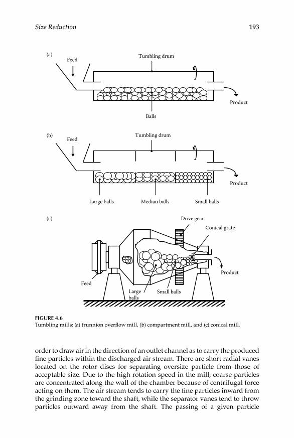
Size Reduction 193
order to draw air in the direction of an outlet channel as to carry the produced fine particles within the discharged air stream. There are short radial vanes located on the rotor discs for separating oversize particle from those of acceptable size. Due to the high rotation speed in the mill, coarse particles are concentrated along the wall of the chamber because of centrifugal force acting on them. The air stream tends to carry the fine particles inward from the grinding zone toward the shaft, while the separator vanes tend to throw particles outward away from the shaft. The passing of a given particle
Product
Feed (a)
(b)
(c)
Tumbling drum
Balls
Product
Feed Tumbling drum
Large balls Median balls Small balls
Small balls Largeballs
Product
Conical grate Drive gear
Feed
Figure 4.6Tumbling mills: (a) trunnion overflow mill, (b) compartment mill, and (c) conical mill.

194 Unit Operations of Particulate Solids
between the separator vanes and out to be discharged depends on which force predominates: the drag exerted by the air or the centrifugal force exerted by the vanes. Finer particles are carried through and discharged, whereas coarser particles return to be reduced even more in the grinding chamber. The particle size of the product may be varied changing the rotor speed and the size or number of the separator fins.
In fluid-energy (jet) mills, the particles of the solid are suspended in a stream of gas and driven along a circular or elliptical duct at high speed. The size reduction of the particles is accomplished, in part, by particle–particle impact and friction. The particles pass through a classifier nozzle when they reach a determined size. The suspending gas is, usually, compressed air or superheated steam, admitted at a pressure of approximately 6900 Pa. Solids are fed near the bottom of the loop through a Venturi injector. Classification of ground particles takes place at the upper bend of the loop. The gas flows around this bend at high-speed projecting coarser particles toward the outer wall and congregating the fines in the vicinity of the inner wall. A discharge opening against the inner wall at this upper part of the loop leads to cyclone separator and a bag collector. Fluid-energy mills are highly efficient when the fed particles are no larger than 150 μm.
Agitation mills are vessels of capacities between 4 and 1000 L, which con-tain a liquid with crushing elements such as balls or sand grains in suspen-sion. The solid to be ground is fed by the upper section and some kind of agitation is applied, while the product is taken by the lower section through a sieve.
Cutting machines that are similar to grinding equipments and produce fine systems with uniform size distributions are known as rotary knife cut-ters. They are used for materials that are too tenacious or too resilient to be broken by compression, impact, or attrition such as rubbers, plastics, or leaves of vegetables and spices. The rotary knife cutters have a very similar design to the hammer mills, since they have a horizontal rotor that spins between 200 and 900 rev/min inside a cylindrical chamber. The rotor has mounted from 2 to 12 hardened steel or stellite knives that pass leaving a very narrow clearing in front of a series of stationary knives. Feed is introduced by the upper section and the product passes through a sieve in a lower opening in order to be collected and withdrawn. The cutting elements are exchangeable according to the specific needs of a process.
example 4.1
A crusher is fed with limestone having particles of 2 cm median equivalent diameter and discharges a product consisting of particles of 0.5 cm median equivalent diam-eter. The equipment operates at a capacity of 1.2 × 10⁴ kg/h consuming a power of 10 hp. If the requirements of the process demand a finer size of the product (0.4 cm of median equivalent diameter) decreasing the capacity to 1.0 × 10⁴ kg/h, determine the theoretical power consumption under the new conditions.

Size Reduction 195
SoluTion
The feed particles can be considered very coarse, and so Kick’s law would be the most appropriate. The starting and final sizes, in average, are of 0.02 and 0.005 m, respectively, while the power is equivalent to 7.46 kW. It is known, also, that the energy of operation is derived from the relation between power and flow rate, that is, E = P/Q, therefore, the constant K for Equation 4.3 may be calculated as follows:
K =
=
7 4612000
0 020 005
0
.
ln.
.
.4 48 1 kWh kg4× /−
Since the new conditions are not significantly different, the constant K may be used in the same relationship to find for the new conditions the power as
P =
( )( . )ln.
..10000 0 000448
0 020 004
= 7 21 kW
Thus, the theoretical power for the new conditions of the comminution operation will be 7.2 kW approximately.
4.3.3 operation of equipment
The diversity of designs of the above-described machinery implies that their operating variables differ quite considerably. While energy require-ments are generally governed by the comminution laws previously dis-cussed, as illustrated in Example 4.1, some other features such as capacity and rotational velocity are particular for each unit and may be related, in some way, to the predominant force performing the reduction action. Two types of equipment with critical particularities of operation would be roller mills and tumbling mills.
In crushing rolls, the angle formed by the tangents to the roll faces at the point of contact between a particle and the rolls is called the angle of nip. It is an important variable for specifying the size of a pair of crushing rolls for a specific duty and is found as follows. Figure 4.7 shows a pair of rolls and a spherical particle just being gripped between them. The radii of rolls and particle are R and r, respectively. The clearance between the rolls is 2d. Line AB passes through the centers of the left-hand roll and the particle, as well as through point C, which is the point of contact between the roll and the par-ticle. As shown in Figure 4.7, if α is the angle between line AB and the hori-zontal, line OE is a tangent to the roll at point C and it makes the same angle α with the vertical. Neglecting gravity, two forces act at point C: the tangen-tial frictional force Ft, having a vertical component Ft cos α, and the radial force Fr, having a vertical component Fr sin α. Force Ft is related to force Fr through the coefficient of friction μ, so Ft = μ′Fr. Force Fr sin α tends to expel

196 Unit Operations of Particulate Solids
the particle from the rolls, while force μ′Fr cos α tends to pull it into the rolls. If the particle is to be crushed:
F Fr r µ α α′ ≥cos sin (4.5)
or
µ α′ ≥ tan (4.6)
When μ′ = tan α, the angle α is half the angle of nip. A simple relationship exists between the radius of the rolls, the size of the feed, and the gap between the rolls. Thus, from Figure 4.7,
cosα = +
R dR r
+
(4.7)
The largest particles in the product would have a diameter 2d and Equation 4.7 provides a relationship between the roll diameter and the size reduction that can be expected in the mill.
From Figure 4.7, it follows that 2R will represent the diameter of the roll Dr, 2r will be the diameter of the feed Df (when the feeding pieces have a proper sphericity Φs), and 2d will be considered the product diameter Dp. Con sidering these definitions, the theoretical volumetric capacity Q of crushing
C
d
O
α
B
E
α FtFt (cos α)
αFr
(sin α)A
Fr
r
α
R + r
R + d
d
R
Figure 4.7Diagram of forces and angle of nip in crushing rolls.
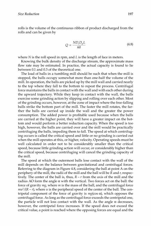
Size Reduction 197
rolls is the volume of the continuous ribbon of product discharged from the rolls and can be given by
Q
ND D L= r p
60 (4.8)
where N is the roll speed in rpm, and L is the length of face in meters.Knowing the bulk density of the discharge stream, the approximate mass
flow rate may be estimated. In practice, the actual capacity is found to lie between 0.1 and 0.3 of the theoretical one.
The load of balls in a tumbling mill should be such that when the mill is stopped, the balls occupy somewhat more than one-half the volume of the mill. In operation, the balls are picked up by the mill wall and carried nearly to the top where they fall to the bottom to repeat the process. Centrifugal force maintains the balls in contact with the wall and with each other during the upward trajectory. While they keep in contact with the wall, the balls exercise some grinding action by slipping and rolling over each other. Most of the grinding occurs, however, at the zone of impact where the free-falling balls strike the bottom part of the mill. The faster the mill rotates, the far-ther the balls are carried up inside the wall and the greater the power consumption. The added power is profitable used because when the balls are carried at the higher point, they will have a greater impact on the bot-tom and would perform a better reduction capacity. When the speed is too high, however, the balls are carried over and the mill would be practically centrifuging the balls, impeding them to fall. The speed at which centrifug-ing occurs is called the critical speed and little or no grinding is carried out when the mill operates at this, or higher, velocity. Operating speeds must be well calculated in order not to be considerably smaller than the critical speed, because little grinding action will occur, or considerably higher than the critical speed, because centrifuging will cancel the grinding capacity of the mill.
The speed at which the outermost balls lose contact with the wall of the mill depends on the balance between gravitational and centrifugal forces. Referring to the diagram in Figure 4.8, considering the ball at point A on the periphery of the mill, the radii of the mill and the ball will be R and r, respec-tively. The center of the ball is, thus, R – r from the axis of the mill and the radius AO form the angle α with the vertical. Two forces act on the ball: the force of gravity mg, where m is the mass of the ball, and the centrifugal force mu2/(R – r), where u is the peripheral speed of the center of the ball. The cen-tripetal component of the force of gravity is mg(cos α), which opposes the centrifugal force. As long as the centrifugal force exceeds the centripetal one, the particle will not loss contact with the wall. As the angle α decreases, however, the centripetal force increases. If the speed does not exceed the critical value, a point is reached where the opposing forces are equal and the

198 Unit Operations of Particulate Solids
particle is nearly to fall. The angle at which this occurs is found by equating the centrifugal and centripetal forces, that is,
mg
muR rcos ( )α = −
2
(4.9)
Transposing for cos α, Equation 4.9 transforms to
cos
( )α = u
R r g
2
− (4.10)
The speed u is related to the speed of rotation by the equation
u N R r= 2π ( )− (4.11)
and, thus, Equation 4.11 can be written as
cos
( )α π= −4 2 2N R rg
(4.12)
A
O
mg cos α
mu2
(R – r)
r
mg
R – r
R
α
Figure 4.8Diagram of forces on balls in a ball mill.

Size Reduction 199
At the critical speed, α = 0, consequently cos α = 1, and N becomes the critical speed Nc. With all these considerations, Equation 4.12 transforms into
N
gR rc = −
12π ( )
(4.13)
Rod mills can produce 5–200 ton/h of material reduced up to about 1 mm sizes, while ball mills can give 1–50 ton/h of fine powder with 70–90% sizes in the range of 70 μm. The total energy requirement for a typical rod mill grind-ing different hard materials is about 5 hp h/ton, whereas for a ball mill, it is approximately 20 hp h/ton. Tube mills and compartment mills normally need somewhat more power than these figures. As the product becomes finer, the capacity of a given mill diminishes and the energy requirement increases.
example 4.2
A roller mill is used to obtain 4900 kg/h of ground bentonite with 960 kg/m3 bulk density. The rollers spin both at 1.5 m/s and are 1.22 m long with 7.6 cm diameter. Empirical measurements have determined that the mill operates at 30% effi-ciency. Calculate the relation of reduction obtained in the operation if the friction coefficient is 0.52.
SoluTion
The relation of reduction is obtained as the relation between equivalent mean diameters of the feed and the product. In order to obtain the median size of the product, Equation 4.8 may be used to transpose the product diameter Dp, that is,
D
CND L
pr
= ( )( )60
It is known that the peripheral speed v and the rotation speed N are related by: v = πDrN, and, therefore, substituting in such relation the rotation speed can be calculated as 188.47 rev/min. On the other hand, since the equations are theoreti-cal, process theoretical capacity is determined as: (4900 kg/h)/0.3 = 16333 kg/h. Using the bulk density, mass flow rate could be transformed into volumetric flow rate, as (16,333 kg/h)/960 kg/m3 = 17.01 m3/h. Furthermore, considering the equiv-alence between seconds and hours, the volumetric capacity of 0.0047 m3/s would be taken to substitute in the above transposed equation. Thus, the product diam-eter Dp is obtained as
Dp 8 6 m 8 cm= = =( . )( )
( . )( . )( . ). .
0 0047 60188 47 0 152 1 22
0 00 0 0
In order to obtain the average median size of the feed, Equation 4.7 could be used, since, as it was previously mentioned, 2r = Df. By using the friction coefficient μ’,

200 Unit Operations of Particulate Solids
according to Equation 4.6 it could be assumed that: μ’ = tan α and the arc tangent of the friction coefficient would give the value of the angle α. By this procedure the value of the angle: α = 27.47°. Knowing this value, cos α can be also known as 0.8872. From Equation 4.7, the radius of the feed particle r is calculated as
rR d
R= + − = + − =cos
. ..
. .α
0 076 0 0040 8872
0 038 0 014 m
Since Da = 2r, Da = 0.028 m = 2.8 cm.Finally, the relation of reduction would, therefore, be
Relation of reduction a
p= = =D
D2 80 8
3 5..
.
Thus, the relation of reduction is 3.5:1, approximately.
example 4.3
Calculate the critical speed in revolution/minute, of a ball mill with an internal diameter of 1200 mm loaded with balls of 70 mm diameter.
SoluTion
Expressed in meters, the radius of the mill and the balls will be 0.6 and 0.035 m, respectively. Therefore, a direct substitution in the Equation 4.13 will lead to
Nc 6625 1 s 39 75 rev min=
−=1
29 81
0 6 0 0350
π.
( . . ). . / ./ =
4.4 Criteria for Selecting Size Reduction Processes
In deciding how to crush or grind a solid material, process engineers should consider factors such as the size distributions of feed and product, the hard-ness and mechanical structure of the feed, the moisture, and the temperature sensitivity of the feed. Regarding the size distributions of the materials, each type of crusher or grinder is intended for a certain size of feed and product. It is usually possible to exercise some control over the size of feed, but some-times it must be taken as it comes. As there is an upper limit on the size that can be accepted by a machine without jamming, if there is an oversized material, a guard screen is needed to keep too large pieces out of the crusher or grinder. In the case of too much undersized material, prescreening the feed can cut the amount which goes through the equipment. For a small-scale operation, such a cut is important as it decreases the capacity required; in a large-scale equipment, though, the undersized particles simply pass

Size Reduction 201
through the throat, where there is always ample room, and so removing them does not greatly affect capacity. Although many criteria and factors may be taken into consideration, paramount factors in designing comminu-tion processes would be
Characteristics of feed material: mechanical and structural; related •to hardness, abrasiveness, size, shape, and so onFeed and discharge control•Moisture•Heat removal or supply•
4.4.1 Characteristics of raw Materials
Regarding the main features of the feed material, the pieces or particles must be adequate in size and shape in order to avoid jamming, entrapment, or general malfunction of the equipment used to accomplish the size reduction. Prior knowledge of the particular structure of the feed material can indicate the type of force most likely to be used in performing the size reduction. If the material is friable or has a crystalline structure, fracture may occur easily along cleavage planes, with larger particles fracturing more easily than smaller ones. In these cases, crushing using compressive forces would be recommended. When few cleavage planes are present, and new crack tips have to be formed, impact and shear forces may be more advisable. There are some solid materials having fibrous structures and hence they are not easily reduced in size by compression or impact. In such cases, shredding or cut-ting may need forces to perform the desired size reduction.
One of the major factors that govern the choice and design of size reduc-tion machines is the hardness of the material to be processed. The greater the hardness, the highest energy consumption and the longer the time in the action zone of the reducing forces. Normally, very hard materials are also very abrasive; so the parts of the equipment in contact with them must be made of special materials. As a general guidance, the hardness is defined in accordance with Mohs’ scale, which is divided into 10 grades of hardness (Chapter 1). As a rule of thumb, using Mohs’ scale, any material would be considered soft when having a value between 1 and 3, medium-hard if pre-senting a value between 3.5 and 5, and hard when showing a value between 5 and 10.
4.4.2 Feeding and Discharge Control
In most comminution processes, maintaining continuous flow of feed and product is a requirement. For this purpose, a pretreatment of the feed by sieving or even by grinding (e.g., coarse crushing or breaking before passing to an intermediate reduction mill) is necessary. The discharge rate should

202 Unit Operations of Particulate Solids
match the feed rate as much as possible, which is normally guaranteed by the assistance of the force of gravity. Sometimes, however, the use of some sort of conveying system to aid either feed or raw materials or discharge of finished products could be necessary. Some comminution equipment may require a very specific discharge system, such as the peripheral discharge devices adapted to certain tumbling or friction mills. In some ultrafine grinding equipment the fine size of the product requires of a fluid, such as air or water, to assist product collection. A suspension stream is, inevitably, created so that a number of separation devices to recover the dry solids, such as cyclones or bag filters, would be required.
4.4.3 Moisture
The presence of moisture can be either beneficial or inconvenient in com-minution processes. It is well known that safety problems are caused by dust formation arising during the dry milling of many solid materials. It is known, for example, that a concentration of fine inert powders over 30 mg/L requires a spark of 100 mJ to cause an explosion. A spark of this magnitude may be caused by an electric failure or by metal–metal accidental colli-sions, common in handling tools. The presence of small quantities of water has been found useful in the suppression of dust. In applications where the presence of moisture is acceptable, water sprays are often used to reduce dust formation. Some other applications allow for large quantities of water to be introduced in the size reduction process; wet milling of corn is a good example of this. On the other hand, in many cases feed moisture content in excess of 2–3% can lead to clogging of the mill with the consequent effect on throughput and efficiency. Agglomeration can also be caused by mois-ture, being undesirable when a free-flowing powder is needed to control feed rate.
4.4.4 Heat generation and removal
As has been stated earlier, comminution is, possibly, the most inefficient unit operation in the material processing industry. The excessive friction presented in most size reduction machines causes increase in heat which can lead to a considerable increase in temperature of the material being processed. There are many materials of biological and organic origin that are normally heat sensitive, and may cause degradation reactions, release of sticky substances, and many other undesirable phenomena. Knowledge of the chemical stability of heat-sensitive materials, as well as some rele-vant physical properties such as their melting temperatures, should be taken into account before deciding the type of machine used for their size reduction. Many crushing and grinding machinery and equipment may, therefore, be equipped with cooling devices such as jackets, coils, and so on.
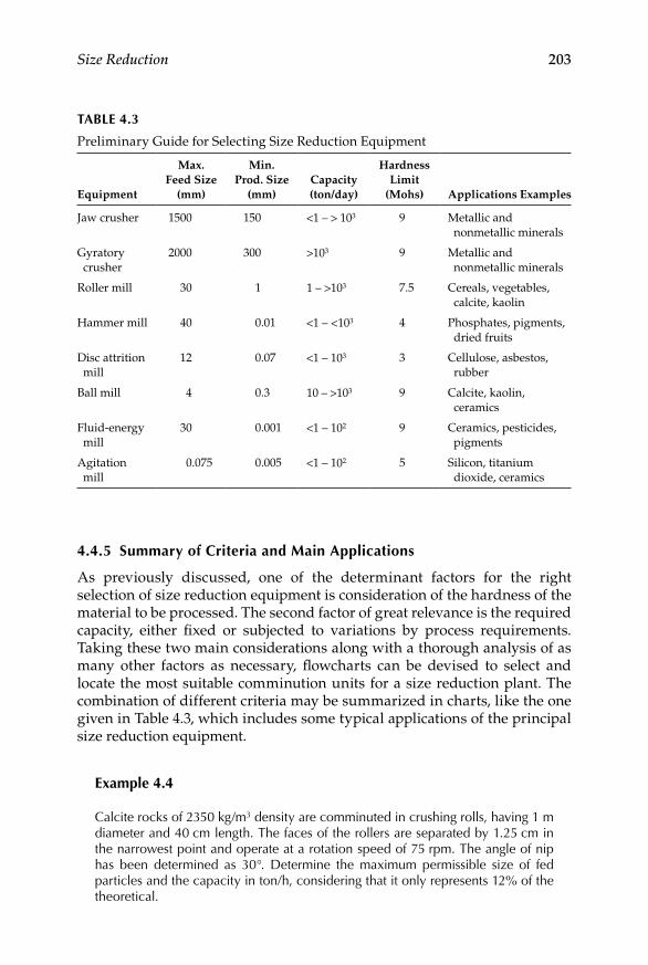
Size Reduction 203
4.4.5 Summary of Criteria and Main applications
As previously discussed, one of the determinant factors for the right selection of size reduction equipment is consideration of the hardness of the material to be processed. The second factor of great relevance is the required capacity, either fixed or subjected to variations by process requirements. Taking these two main considerations along with a thorough analysis of as many other factors as necessary, flowcharts can be devised to select and locate the most suitable comminution units for a size reduction plant. The combination of different criteria may be summarized in charts, like the one given in Table 4.3, which includes some typical applications of the principal size reduction equipment.
example 4.4
Calcite rocks of 2350 kg/m3 density are comminuted in crushing rolls, having 1 m diameter and 40 cm length. The faces of the rollers are separated by 1.25 cm in the narrowest point and operate at a rotation speed of 75 rpm. The angle of nip has been determined as 30°. Determine the maximum permissible size of fed particles and the capacity in ton/h, considering that it only represents 12% of the theoretical.
Table 4.3
Preliminary Guide for Selecting Size Reduction Equipment
Equipment
Max. Feed Size
(mm)
Min. Prod. Size
(mm)Capacity (ton/day)
Hardness Limit
(Mohs) Applications Examples
Jaw crusher 1500 150 <1 – > 103 9 Metallic and nonmetallic minerals
Gyratory crusher
2000 300 >103 9 Metallic and nonmetallic minerals
Roller mill 30 1 1 – >103 7.5 Cereals, vegetables, calcite, kaolin
Hammer mill 40 0.01 <1 – <103 4 Phosphates, pigments, dried fruits
Disc attrition mill
12 0.07 <1 – 103 3 Cellulose, asbestos, rubber
Ball mill 4 0.3 10 – >103 9 Calcite, kaolin, ceramics
Fluid-energy mill
30 0.001 <1 – 102 9 Ceramics, pesticides, pigments
Agitation mill
0.075 0.005 <1 – 102 5 Silicon, titanium dioxide, ceramics
204 Unit Operations of Particulate Solids
SoluTion
As in the case of Example 4.2, in order to calculate the maximum permissible size of feed, the transposed form of Equation 4.7 could be used, considering that the angle α represents half the angle of nip. Thus: cos α = cos(15°) = 0.9659. On the other hand, the radius of the roller, R, is 0.5 m, while the dimension d represents half the distance between rollers, that is, 0.00625 m. Substituting, then in the transposed form of Equation 4.7,
r r= + = = =0 5 0 006250 9659
0 5 0 0 0 0. .
.. . , : .− ∼24 m therefore Da 2 48 m 5 cm
Equation 4.8 can be used to compute the theoretical volumetric flow rate. Substituting all the terms,
Q = =( )( )( . )( . ). /
75 1 0 0125 0 3860
0 00625 m s3
Since real capacity only represents 12% of theoretical, in reality the capacity would only be 0.00075 m3/s. Also, the answer is required in ton/h, so using the density of the material in order to transform to mass flow: (0.00071 m3/s) (2350 kg/m3) = 1.7625 kg/s. Finally, transforming to kg/h and then to ton/h, the required capacity of 6.345 ton/h is obtained. Thus, the results are maximum permissible size of fed particles in average ≈ 5 cm; optimum capacity ≈ 6.3 ton/h.
4.5 Laboratory Exercise: Determination of Reduction Relations Using a Hammer Mill
4.5.1 introduction
It has been argued that hammer mills constitute the most efficient comminu-tion machines available for different size reduction purposes. Their relations of reduction are, therefore, considered among the top within the range of size reduction equipment. The object of this experiment is to study the fac-tors affecting the performance of a hammer mill using the reduction ratio obtained as criteria.
4.5.2 equipment and Materials
Laboratory-scale hammer mills are available from a number of equipment manufacturers. Any laboratory-scale unit would be suitable for the laboratory exercise. Suggested raw materials are granulated sugar and granulated salt.

Size Reduction 205
4.5.3 instruments
Standard set of sieves as particle size analyzers.
4.5.4 Screen analysis
Measure the particle size distributions of feed materials and final products performing a screen analysis, and determine the mean particle sieve diameter as described in Chapter 2 (Section 2.7).
4.5.5 operation of the Hammer Mill
Select an appropriate amount of a raw material according to mill size •and screen it through a set of sieves so as to determine the size of distribution and average size, according to the procedure mentioned in the previous section.Select one of the screen plates of the mill, perhaps one with the finest •holes, and screw it into position. Start the motor and read the watt-meter over a short period. This reading will give a measure of the power consumption with the machine running idle.Introduce a weighed quantity of the material, according to specific •instruction of the equipment, and keep a constant rate sufficient to maintain the ammeter reading constant, so as to guarantee efficient use of energy in the run.Collect the product for the entire run and carry out a screen analysis •of the product, similar to the one carried out before for the feed material.Repeat the experiment using the second feed material.•Determine the reduction relation ratio for the two experiments.•
4.5.6 Calculations and report
Compare the reduction relations for the tested materials and elabo-•rate a discussion on significant differences, if any, of these two materials.Perform a literature search to find out whether similar materials com-•minuted in different size reduction equipment, would present differ-ent reduction relations. Analyze and discuss on these findings.Present a complete written report, according to scientific report •guidelines, either given by the instructor or consulted in the litera-ture. Include graphs, charts, and calculations carried out. Include, as an important part of the report, the discussion elaborated from the literature survey previously performed.

206 Unit Operations of Particulate Solids
PROBLEMS
1. 150 ton/day of pyrite of 2 mm average size need to be milled to an average size of 0.1 mm, using any of three ball mills of 12.5, 25, and 50 cm in diameter, respectively, all with balls of 5 cm of diameter as the pulverizing medium. Which mill would be more adequate to perform the duty knowing that, everything included, 10 kW/rpm are approximately needed to operate? The value of K has been reported as 2.5 × 10⁻⁸ kW h m/kg, and the process is 30% efficient.
2. 120 ton/h of clay having an average size of 101.6 mm (4 in.) is going to be reduced to an average size of 3.175 mm (1/8 of an in.). If the work index Ei has been estimated as 16.4, calculate the power neces-sary to crush the material, as well as the power needed to crush it even more, and hence the final size would be of 1 mm average size.
3. A material is fed to a pair of crushing rollers, each one rotating at the same speed of 1.25 m/s. Each roller is 1.5 m long with 7.5 cm diameter. The product has a density of 1050 kg/m3 and is dis-charged at a flow of 5000 kg/h. If the measured flow is 30% of the theoretical value, calculate the relation of reduction of the process.
References
Beddow, J. K. and Meloy, J. K. 1980. Testing and Characterization of Powders and Fine Particles. London: Heyden and Son.
Bond, F. C. 1952. The third theory of comminution. AIME Transaction 193: 484–494.Bond, F. C. 1963. Some recent advances in grinding theory and practice. British
Chemical Engineering 8: 631–634.Herdan, G. 1960. Small Particle Statistics. London: Butterworths.Kick, F. 1885. Das Gesetz der Proportionalen Widerstande und Sein Enwendung. Leibzig:
Artuz Felix.McCabe, W. L., Smith, J. C., and Harriot, P. 2005. Unit Operations in Chemical Engi-
neering, 7th Ed. New York, NY: McGraw-Hill.Richardson, J. F., Harker, J. H., and Backhurst, J. R. 2002. Coulson & Richardson’s
Chemical Engineering, Vol. 2. Oxford: Butterworth-Heinemann.Rittinger, P. R. 1867. Lehrbauch der Aufbereitungskunde. Berlin: Ernst and Korn.

207
5Size Enlargement
5.1 Introduction: Agglomeration Processes
Size enlargement operations are used in the materials processing industry with different aims, such as improving handling and flow, reducing losses, producing specific shapes, boosting appearance, and so on. Processes involv-ing any kind of size enlargement receive diverse denominations including compaction, granulation, encapsulation, pelletizing, agglomeration, and sin-tering. Some of these terms may represent synonyms referring to the same operation but applied in different industries, while others define operations employed in very specific processes, such as sintering in metallurgy. A generic classification could divide size enlargement operations into two main categories: those operations in which the enlargement objective is to control functional properties such as rehydration, and those in which the enlargement objective is to produce defined forms such as tablets or pellets. In a broad sense the former could be defined as tumbling agglomeration, whereas the latter could be referred to as pressure compaction.
5.2 Aggregation Fundamentals: Strength of Agglomerates
Agglomeration may be defined as the process of bonding individual parti-cles in a random way, in order to end with an aggregate considerably larger in size and with a porous structure. As previously mentioned, agglomera-tion comprises a variety of operations in which particles are grouped for different purposes (Green and Perry, 2008). Figure 5.1 shows some common mechanisms of agglomerate binding that originate in coordination systems, much as those observed in crystallization arrangements (Pietsch, 1991). Each particle interacts with neighboring particles, while points of interaction may be kept together by physical contact or by attractive forces due to the proxim-ity of such points. The number of interaction sites of each particle within the agglomerate is known as coordination number. In reality, agglomerates

208 Unit Operations of Particulate Solids
consist of a huge number of particles, which makes it difficult to estimate their coordination number. Indirect measurement of the coordination number can be made as a function of other properties of the agglomerate. In regular packs of monosized spherical particles the coordination number k and the porosity or void volume ε, are related by
kε ≈ π (5.1)
Equation 5.1 gives an appropriate approximation of coordination numbers for ideal agglomerate structures. Table 5.1 lists coordination numbers calcu-lated from Equation 5.1 and compares them with coordination numbers of ideal structures, like some illustrated in Figure 5.2.
(a) (b) (c)
(d) (e) (f)
Figure 5.1Different binding mechanisms in agglomeration: (a) partial melting sinter bridges, (b) chemi-cal reaction hardening binders, (c) liquid bridges hardening binders, (d) molecular and like-type of forces, (e) interlocking bonds, and (f) capillary forces.
Table 5.1
Geometric Arrangement, Porosity, and Coordination Number of Packings of Monosized Particles
Geometric Arrangement Porosity (ε)Coordination Number (π/ε) k
Cubic 0.476 6.59 6Orthorhombic 0.395 7.95 8Tetragonal-spheroidal 0.302 10.39 10Rhombohedral (pyramidal) 0.260 12.08 12Rhombohedral (hexagonal) 0.260 12.08 12

Size Enlargement 209
A generic relationship to describe the tensile strength of agglomerates σt held together by binding mechanisms acting at the coordination points is
σ ε
πt = − =∑1 12k
A x
xi
i
n( , ...)
(5.2)
where Ai is the adhesive force due to a particular binding mechanism and x is the representative size of the particles forming the agglomerate.
Substituting Equation 5.1 into Equation 5.2, the following relation is obtained:
σ ε
εt = − =∑1 12
A x
xi
i
n( , ...)
(5.3)
A further simplification results because many binding mechanisms are a function of the representative particle size x and thus
σ ε
εt = − =∑1 1A x
xi
i
n( , ...)
(5.4)
The ellipses within parentheses in Equations 5.2 through 5.4 indicate that Ai is also a function of other, unknown, parameters.
(a) (b) (c)
(d) (e) (f)
Figure 5.2Packings of mono-sized spherical particles: (a) cubic, (b) and (c) orthorhombic, (d) tetragonal-spheroidal, (e) rhombohedral (pyramidal), (f) rhombohedral (hexagonal).
210 Unit Operations of Particulate Solids
When liquid bridges have formed at the coordination points, Ai depends on the bridge volume and the wetting characteristics represented by the wetting angle. There are models available for predicting adhesion forces of various types (Pietsch, 1991), but Ai might be of different magnitude at each of the many coordination points, due to roughness or microscope structure of particulates forming the agglomerates.
The representative particle size most appropriate to describe the agglom-eration process is the surface equivalent diameter, xsv (Table 2.5), because porosity is surface dependant. As described in Chapter 2, such diameter is the size of a spherical particle which, if the powder consisted of only these particles, would have the same specific surface area as the actual sample. When determining the specific surface area, methods must be chosen that only measure the outer particle surface excluding the accessible inner sur-face due to open particle porosity. One of these recommended methods is permeability, also discussed in Chapter 2.
From the previous paragraphs, it can be gathered that the strength of agglomerate structures held together by bonding mechanisms is highly dependent on porosity and particle size, or, more properly, specific surface area. The relationship would be inversely proportional in both cases, that is, higher strength at lower porosities and lower surface areas. Tumbling agglomeration is often aided by adding small quantities of liquids, generally water. Depending on the degree of moisture, three states of agglomerate sta-bility can be identified: pendular state when moisture is located only in the contact points of particles, funicular state when a layer of moisture covers the surface of particles, and capillary state when moisture fills the voids of a bed of particles (Green and Perry, 2008). Agglomerates that are completely filled with liquid obtain strength from the negative capillary pressure in the structure. When liquid bridges help maintaining the stability of an agglom-erate, its strength can be calculated by
σ ε
εα
δts
= −
cx f
1( )
(5.5)
where c is a correction factor, α is the surface tension of the liquid, xs is the surface equivalent diameter of the particle, and f (δ) is a constant related to the angle of contact of particles. Reported values of constant c vary between 2.8 and 8.0, depending on the degree of moisture trapped by agglomerates with the maximum value of 8.0 corresponding to the capillary state. Regarding values of f (δ), they also correlate to moisture content of agglomer-ates with a maximum value of unity corresponding to the capillary state.
For high-pressure agglomeration and the effect of matrix binders general formulas have not yet been developed. It can be considered, however, that the effects of variables would follow the trend described before, with poros-ity, particle surface, contact area, and adhesion, all playing an important role.
Size Enlargement 211
For nonmetallic powders, the following equation can be used to evaluate the needed applied pressure p to agglomerate:
log Rp mV b= + (5.6)
where VR represents the relationship V/Vs, being V the compacted volume at a given pressure and Vs the volume of the solid material to be compacted; m and b are correlation constants.
example 5.1
Particles of 0.1 μm diameter are going to be agglomerated by mobile liquid bridges mechanism using water as the bonding agent. Calculate the strength of the agglomerate when the voids of the aggregates are totally wet. The porosity of the agglomerates is 0.65 and the surface tension of water is 72.8 dyne/cm.
SoluTion
The agglomerate corresponds to the capillary state, with the voids completely wet. As previously mentioned, the values for such a case for c and f(δ) on Equation 5.5 are 8.0 and 1.0, respectively.
Substituting, thus, directly in Equation 5.5:
σ t dy= −
×
= ×−8 01 0 65
0 6572 8
1 10 13 92 105
6.( . )
( . ).
( )( ). nne cm/ 2
The strength of the agglomerate is, therefore, 3.92 × 10⁶ dyne/cm2.
example 5.2
Calculate the volume of a tablet made of compressed ceramic powder by pressing it in a 54 cm3 cavity applying a pressure of 316 MPa. The process of pressurization followed the model described by Equation 5.6, and the correlation constants m and b were determined as −4.402 and 4.1157, respectively.
SoluTion
Substituting values directly on Equation 5.6, and then transposing VR from such equation, the volumes relationship would be obtained as
log( ) . ( ) .316 4 402 4 1157= − +VR
VR = −
−=( . . )
..
2 4997 4 11574 402
0 367
212 Unit Operations of Particulate Solids
VR represents the volume of 1 compressed tablet of volume V, and so the solid before compression would be Vs. Assuming that the uncompressed solid occupies the total volume of the press cavity (54 cm3), the volume of the tablet can be calculated as
V V V= = × = ×− −R s m m( . )( . ) .0 367 5 4 10 1 98 105 3 5 3
Thus, the tablet volume would be 20 cm3 approximately.
5.3 Agglomeration Methods
With few exceptions, agglomeration methods can be classified into two groups: tumble/growth agglomeration and pressure agglomeration. Also, agglomerates can be obtained using binders or in a binderless manner. The tumble/growth method produces agglomerates of approximate spherical shape by buildup during tumbling of fine particulate solids, the resulting granules are at first weak and require binders to facilitate formation, and posttreatment is needed to reach final and permanent strength. On the other hand, products from pressure agglomeration are made from particulate materials of different sizes, and they are formed without the need of binders or posttreatment acquiring immediate strength.
5.3.1 Tumbling agglomeration
The mechanism of tumble/growth agglomeration is illustrated in Figure 5.3. As shown, the overall growth process is complex and involves both disinte-gration of weaker bonds and reagglomeration by abrasion transfer and coalescence of larger units (Cardew and Oliver, 1985). Coalescence occurs at the contact point when, at impact, a binding mechanism develops which is stronger than the separating forces. Additional growth of the agglomerate may proceed by further coalescence, or by layering, or both. The most impor-tant and effective separation force counteracting on the bonding mechanism is the weight of the solid particle. For particles below 10 μm approximately, the natural attraction forces, such as molecular, magnetic, and electrostatic, become significantly larger than the separation forces due to particle mass and external influences. In such a way, natural agglomeration occurs. The mechanism of tumble/growth agglomeration is similar to that of natural agglomeration. The particles to be agglomerated are larger, however, and so the particle-to-particle adhesion would need to be increased by addition of binders, such as water or other more viscous liquids, depending on the prop-erties of particles being agglomerated and the required strength of the agglomerate structure. On the other hand, the collision probability may be enhanced by providing higher particle concentration.
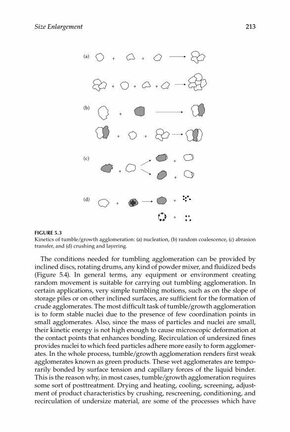
Size Enlargement 213
The conditions needed for tumbling agglomeration can be provided by inclined discs, rotating drums, any kind of powder mixer, and fluidized beds (Figure 5.4). In general terms, any equipment or environment creating random movement is suitable for carrying out tumbling agglomeration. In certain applications, very simple tumbling motions, such as on the slope of storage piles or on other inclined surfaces, are sufficient for the formation of crude agglomerates. The most difficult task of tumble/growth agglomeration is to form stable nuclei due to the presence of few coordination points in small agglomerates. Also, since the mass of particles and nuclei are small, their kinetic energy is not high enough to cause microscopic deformation at the contact points that enhances bonding. Recirculation of undersized fines provides nuclei to which feed particles adhere more easily to form agglomer-ates. In the whole process, tumble/growth agglomeration renders first weak agglomerates known as green products. These wet agglomerates are tempo-rarily bonded by surface tension and capillary forces of the liquid binder. This is the reason why, in most cases, tumble/growth agglomeration requires some sort of posttreatment. Drying and heating, cooling, screening, adjust-ment of product characteristics by crushing, rescreening, conditioning, and recirculation of undersize material, are some of the processes which have
+ +
+ + +
(a)
+
+ +
(b)
+
+
+
(c)
+ +
+
(d)
Figure 5.3Kinetics of tumble/growth agglomeration: (a) nucleation, (b) random coalescence, (c) abrasion transfer, and (d) crushing and layering.
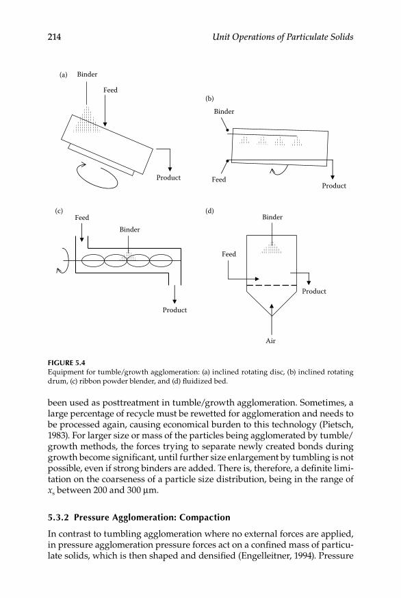
214 Unit Operations of Particulate Solids
been used as posttreatment in tumble/growth agglomeration. Sometimes, a large percentage of recycle must be rewetted for agglomeration and needs to be processed again, causing economical burden to this technology (Pietsch, 1983). For larger size or mass of the particles being agglomerated by tumble/growth methods, the forces trying to separate newly created bonds during growth become significant, until further size enlargement by tumbling is not possible, even if strong binders are added. There is, therefore, a definite limi-tation on the coarseness of a particle size distribution, being in the range of xs between 200 and 300 μm.
5.3.2 Pressure agglomeration: Compaction
In contrast to tumbling agglomeration where no external forces are applied, in pressure agglomeration pressure forces act on a confined mass of particu-late solids, which is then shaped and densified (Engelleitner, 1994). Pressure
Binder
Feed
Product
Binder
FeedProduct
FeedBinder
Product
Air
Feed
Binder
Product
(a)
(b)
(c) (d)
Figure 5.4Equipment for tumble/growth agglomeration: (a) inclined rotating disc, (b) inclined rotating drum, (c) ribbon powder blender, and (d) fluidized bed.

Size Enlargement 215
agglomeration is normally carried out in two stages. The first one comprises a force rearrangement of particles due to a little applied pressure while a second step consists on a steep pressure rise during which brittle particles break and malleable particles deform plastically (Pietsch, 1994). The mecha-nism of pressure agglomeration is illustrated in Figure 5.5. There are two important phenomena that may limit the speed of compaction and, there-fore, the capacity of the equipment: compressed air in the pores and elastic spring-back. Both can cause cracking and weakening which, in turn, may lead to destruction of the pressure-agglomerated products. The effect of these two phenomena can be reduced if the maximum pressure is main-tained for some time, known as dwell time prior to its release.
Pressure agglomeration can be performed employing a low-, a medium-, or a high-pressure mode. When utilizing low- or medium-pressure agglomera-tion, relatively uniform agglomerates can be obtained. Under these condi-tions, the porosity of the feed material is changed but no change in particle size or shape occurs. The feed mixture is often prepared with fine particles and binders giving, thus, a sticky mass which may be formed by forcing it through holes in differently shaped screens or perforated dies. Agglomeration and shaping are, therefore, due to pressure forcing the material through the holes, as well as by frictional forces. High-pressure agglomeration is charac-terized by a large degree of densification, resulting in low product porosity. Typically, the products from high-pressure agglomeration feature high strength immediately after discharge from the equipment. To increase strength a bit further, addition of small amounts of binders or use of post-treatment methods are possible. High-pressure agglomeration is considered
Elasticspringback
Compacted
(Plastic)(Brittle)
Bulk Densified
Time
Pres
sure
Figure 5.5Mechanism of pressure agglomeration.

216 Unit Operations of Particulate Solids
a versatile technique by which particulate material of any kind and size, that is, from nanometers to centimeters, can be successfully processed under certain conditions.
Pressure agglomeration can be carried out in different types of equipment. Generally, low- and medium-pressure agglomeration is achieved in extrud-ers including the screen extruder, the screw extruder, and the intermeshing gears extruder. On the other hand, high-pressure agglomeration is performed in presses such as the punch-and-die press, the compacting roller press, and the briquetting roller press. Low- and medium-pressure agglomeration yield relatively uniform agglomerates of elongated spaghetti-like or cylindrical shape, whereas high-pressure agglomeration produces pillow- or almond-like shapes. Figure 5.6 presents equipment used for low- and medium- pressure agglomeration, while Figure 5.7 illustrates some common machinery for high-pressure agglomeration.
5.3.3 equipment operation Variables
On tumbling agglomeration, an important factor in operation would be the quantity of bonding liquid to add to the process in order to obtain resistant and functional agglomerates. On the other hand, due to agglomerates being formed as a consequence of gentile particle contact in the tumbling process, rotation speed of the agglomerating units would also be crucial. Optimum rotation speed should guarantee sufficient time to promote interparticle contact, but not so much time as to risk agglomerate stability.
(a.1) (a.2)
(a.3)
(b.1) (b.2)
(b.3)
Figure 5.6Equipment used for (a) low- and (b) medium-pressure agglomeration: (a.1) screen extruder, (a.2) basket extruder, (a.3) cylindrical-die screw extruder, (b.1) flat-die extruder, (b.2) cylindrical -die extruder, (b.3) intermeshing-gears extruder.

Size Enlargement 217
Appropriate liquid content, expressed as fraction X, for an optimum agglomeration process, can be represented by the following relation:
X =
+ −
11 1( ) ( )( )ε ρ ε ρs
(5.7)
where ε is the porosity of the material, ρs is the solid density, and ρ is the liquid density.
In terms of optimum rotation speed of tumbling agglomeration units, normally rotating drums, this can be calculated by
N
D= 42 3.
(5.8)
where N is the rotational speed in rev/min, and D is the diameter of the drum in m.
For rotating discs used in agglomeration purposes, the power P and the mass flow rate Q can be calculated by the following equations:
P k D= 12( ) (5.9)
Q k D= 22( ) (5.10)
where k1 and k2 are empirical constants, while D is the disc diameter.
Screw
RollFeed
Product
(a)
Feed
Screw
Roll
Product
(b)
Figure 5.7Equipment used for high-pressure agglomeration: (a) compacting roller press, (b) briquetting roller press.
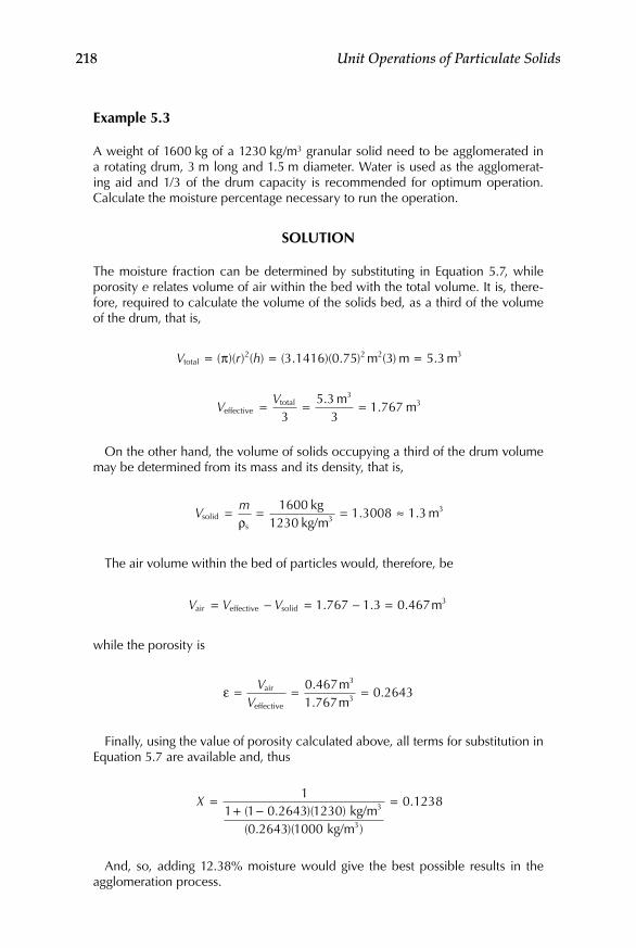
218 Unit Operations of Particulate Solids
example 5.3
A weight of 1600 kg of a 1230 kg/m3 granular solid need to be agglomerated in a rotating drum, 3 m long and 1.5 m diameter. Water is used as the agglomerat-ing aid and 1/3 of the drum capacity is recommended for optimum operation. Calculate the moisture percentage necessary to run the operation.
SoluTion
The moisture fraction can be determined by substituting in Equation 5.7, while porosity e relates volume of air within the bed with the total volume. It is, there-fore, required to calculate the volume of the solids bed, as a third of the volume of the drum, that is,
V r htotal m m m= = =( )( ) ( ) ( . )( . ) ( ) .π 2 2 2 33 1416 0 75 3 5 3
V
Veffective
total mm= = =
35 3
31 767
33.
.
On the other hand, the volume of solids occupying a third of the drum volume may be determined from its mass and its density, that is,
V
msolid
s
kgkg/m
m= = = ≈ρ
16001230
1 3008 1 333. .
The air volume within the bed of particles would, therefore, be
V V Vair effective solid m= − = − =1 767 1 3 0 467 3. . .
while the porosity is
ε = = =V
Vair
effective
mm
0 4671 767
0 26433
3
.
..
Finally, using the value of porosity calculated above, all terms for substitution in Equation 5.7 are available and, thus
X = =11 1 0 2643 1230
0 2643 1000
0 12383
3
+ −( . )( )( . )( )
.kg/m
kg/m
And, so, adding 12.38% moisture would give the best possible results in the agglomeration process.
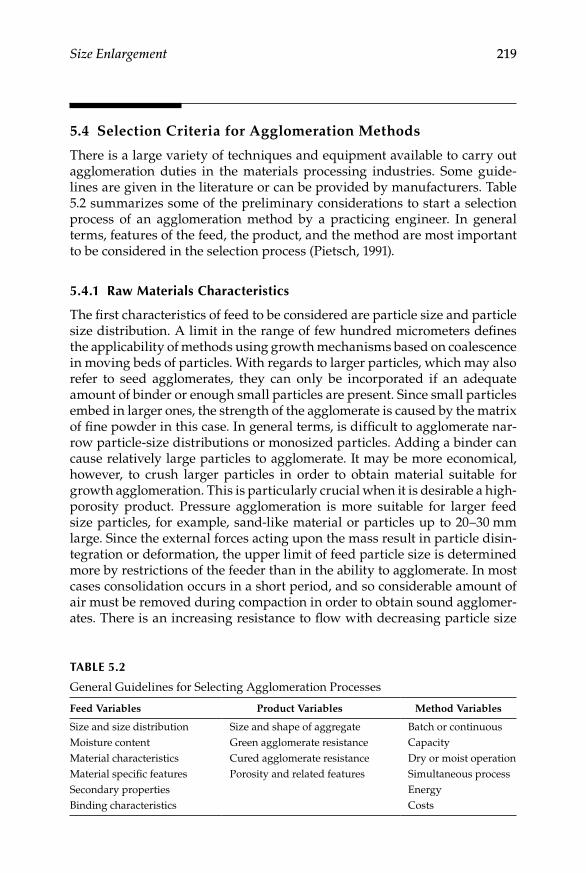
Size Enlargement 219
5.4 Selection Criteria for Agglomeration Methods
There is a large variety of techniques and equipment available to carry out agglomeration duties in the materials processing industries. Some guide-lines are given in the literature or can be provided by manufacturers. Table 5.2 summarizes some of the preliminary considerations to start a selection process of an agglomeration method by a practicing engineer. In general terms, features of the feed, the product, and the method are most important to be considered in the selection process (Pietsch, 1991).
5.4.1 raw Materials Characteristics
The first characteristics of feed to be considered are particle size and particle size distribution. A limit in the range of few hundred micrometers defines the applicability of methods using growth mechanisms based on coalescence in moving beds of particles. With regards to larger particles, which may also refer to seed agglomerates, they can only be incorporated if an adequate amount of binder or enough small particles are present. Since small particles embed in larger ones, the strength of the agglomerate is caused by the matrix of fine powder in this case. In general terms, is difficult to agglomerate nar-row particle-size distributions or monosized particles. Adding a binder can cause relatively large particles to agglomerate. It may be more economical, however, to crush larger particles in order to obtain material suitable for growth agglomeration. This is particularly crucial when it is desirable a high-porosity product. Pressure agglomeration is more suitable for larger feed size particles, for example, sand-like material or particles up to 20–30 mm large. Since the external forces acting upon the mass result in particle disin-tegration or deformation, the upper limit of feed particle size is determined more by restrictions of the feeder than in the ability to agglomerate. In most cases consolidation occurs in a short period, and so considerable amount of air must be removed during compaction in order to obtain sound agglomer-ates. There is an increasing resistance to flow with decreasing particle size
Table 5.2
General Guidelines for Selecting Agglomeration Processes
Feed Variables Product Variables Method Variables
Size and size distribution Size and shape of aggregate Batch or continuousMoisture content Green agglomerate resistance CapacityMaterial characteristics Cured agglomerate resistance Dry or moist operationMaterial specific features Porosity and related features Simultaneous processSecondary properties EnergyBinding characteristics Costs

220 Unit Operations of Particulate Solids
due to the smaller pore radii. For this reason, fine bulk solids of about 150 μm or less, can only be agglomerated by pressure methods if certain precondi-tions, such as low speed and dwell time, are established.
Free moisture can play an important role in growth agglomeration by coalescence. In such a case, moisture provides the binder or prevailing binder mechanism. The maximum volume of liquid must not be more than 95% of anticipated agglomerate porosity. Wet agglomeration is sensitive to this limit because a small excess of moisture will cause the entire mass to turn to mud. For the case of fluidized-bed agglomerators, which may also act as driers, the moisture content is less critical because it has to be high enough to make the feed pumpable. In pressure agglomeration moisture must be kept low being, sometimes, a precondition a completely dry feed. Due to the extreme com-pression forces in high-pressure agglomeration, crushing, rearrangement, and deformation of the solid take place and result in a considerable reduc-tion of porosity. Excess water is either squeezed out or remains in the mass as an incompressible component, with the effect of resultant low strength of the agglomerate.
Material characteristics such as chemical properties, particle density, brit-tleness, elasticity, plasticity, wettability, and abrasivity, all play important roles in the choice of an agglomeration method. Particular chemical charac-teristics may be necessary to bring about the required chemical bonding, or may be incompatible with certain conditions of a method, such as addition of water or other liquids in most growth agglomeration techniques. Density of the feed particles determines particle weight and other field forces which may be counteractive to addition by coalescence. Brittleness, elasticity, plas-ticity, and abrasivity are most important for pressure agglomeration and of less concern for growth methods. Wettability, on the other hand, is para-mount for all agglomeration methods using surface tension and capillary forces in the growth regime. Wetting of particle surfaces is a requirement for green strength.
Bulk properties, such as bulk density and flowability, as well as tempera-ture, can be adjusted prior to agglomeration in order to improve size enlarge-ment. High bulk density and unacceptable flowability are sometimes correlated by using two agglomeration methods in series. To reduce negative impact of these two factors, some sort of preconditioning should be neces-sary. For example, in some compacting processes fine feed powders are preagglomerated to reduce the compaction stroke and improve the flow of feed into a die. This increases the speed of the turret for rotary table tablet-ting machines. At the same time, this technique avoids segregation of the feed mix by stabilizing the blend in a granular form. Finally, the binding features of a given material must be considered for a possible agglomeration process. The binding characteristics should be assessed in order to decide whether agglomeration can be carried out binderless, due to the presence of an inherent binder in the material, or with the addition of binders such as water and some other liquids.
Size Enlargement 221
5.4.2 Product Properties
Some properties such as shape, dimensions, and particle size distribution of the agglomerated product, also influence proper selection of a suitable method. Agglomerated products are normally expected to improve in prop-erties such as free flowing characteristics or dust-free features. Granular, free-flowing, dust-free products can be manufactured using almost all meth-ods of size enlargement. The task of narrowing down the size distribution of the discharge is done by screening out under- and oversized components. While the fines are recirculated to the agglomeration unit, oversized parti-cles are crushed and either rescreened or directly recirculated with the fines. Granular products can also be obtained by crushing and screening large agglomerates using criteria such as product porosity, product density, solu-bility, or reactivity.
The shape of the product is another important property. Spherical prod-ucts are often desirable from an agglomeration operation, and such shape can be obtained using all growth agglomeration methods. Contrastingly, spherical products cannot normally be obtained with high-pressure agglom-eration, unless extremely accurate feed control can be established. By using some types of pressure agglomeration equipment, such as tabletting machines, approximations to the spherical shape such as pillow-, lens-, or almond-shaped compacts can be obtained.
In terms of strength, such property is relevant for the final product, but also plays a role during the size enlargement operation. In growth agglom-eration green agglomerates are formed first and then must be cured to obtain permanent bonding. A weak state could exist when the binding mechanism of the green agglomerate disappears before the permanent, cured bond sets in. Unless large amount of matrix binders are used, or agglomerates are cured at extremely high temperatures or by some chemical reaction, growth agglomeration products will be normally weaker than pressure agglomera-tion ones.
Pertaining porosity, different strength levels develop primarily because agglomerates growing by coalescence feature higher porosity than those from pressure agglomeration. Materials which may disperse easily, and are only agglomerated to improve handling of the intermediate product, should just have enough strength to survive their short existence. In some other cases a large specific surface is more important than high density and strength. Normally, an increase in external forces acting on the particulate matter during size enlargement will cause porosity and related characteris-tics to decrease, and density and strength to increase.
5.4.3 Technique options
Agglomeration processes can be carried out in a batch or a continuous man-ner, depending on specific requirements and applications. Batch modes are
222 Unit Operations of Particulate Solids
generally low in capacity, but are characterized by a better control than that exercised in a continuous process. Most large-volume applications operate in a continuous form, but may be accompanied by significant variations in quality. In growth agglomeration uncontrolled buildup must be removed, whereas in pressure agglomeration worn parts must be replaced. Most of the growth methods are wet processes using bind liquids for forming green agglomerates, while, normally, high-pressure techniques are operated as dry processes. Agglomeration can be sometimes carried out simultaneously with some other process. Simultaneous processing happens in mixer–gran-ulators, granulator–driers, or even mixer–granulator–driers. Mixers are often also granulators in which both processes occur in different zones. In fluidized-bed granulators, however, agglomeration and drying can take place simultaneously.
Agglomeration shows potential for diverse applications such as recycling of wastes containing valuable ingredients or disposal of particulate wastes without value in an environmentally safe and acceptable way. These applica-tions cannot always find economic justification as they must be typically per-formed in compliance with legislation. Finely divided particulate material is often released to the environs in many dry-operated processes. Often, these fines are precipitated or removed by pollution control devices, but recon-tamination of the environment is an obvious concern and is normally regu-lated. In these cases, agglomeration methods can be employed to obtain a size-enlarged material in order to handle and dispose it in a convenient way. Since, in most cases, one of the reasons for size enlargement is improvement of material handling, an agglomeration facility must be located near the par-ticulate solid source. A suitable method must consider, therefore, the avail-ability and cost of utilities and ancillary devices, such as binders or energy sources when wet granulation may need these requirements. Sometimes, since disposal may represent the main aim of the process, the same task may be accomplished using roller presses for dry compaction, and granulation by crushing and screening.
5.5 Design Aspects of Agglomeration Processes
Agglomeration processes consist on varied operations within a complete system aimed at obtaining a desired product. Mixing and screening are two common operations which are part of an agglomeration process. There are some other varied posttreatments, such as those previously mentioned that are used, mainly, to give strength to the agglomerate.
In tumble/growth agglomeration, if more than one feed powder is treated, the components must be metered and premixed. Homogenization may also be necessary due to the risk of selective agglomeration as the particulates
Size Enlargement 223
fed would involve many different sizes. During mixing, some of the liquid or dry binders could be added. It is also possible to feed all or part of the recycle into the mixer. Aeration of the premixed material is an important factor, so particles will be loose and able to move randomly, in order to pick up binder and agglomerate upon impact. A metered addition to the agglom-erating equipment improves and accelerates agglomerate growth by seed-ing the charge. This is because recycle, despite its representing undersize product, consists largely of somewhat preagglomerated material. Control of the growth mechanism also requires addition of some of the liquid or dry binders in the agglomeration unit. Tumbling equipment produces green agglomerates that are better bonded by liquids. The agglomerate sizes and shapes are very varied ranging within wide limits. Sometimes it is possible to screen the green agglomerates and feed only a narrow particle size distri-bution to the posttreatment stage. The moist recycle should be sent directly to the agglomeration unit. Green agglomerates are often weak and sticky, so they tend to blind screen quite easily. For this reason, separation of over- or undersized material at this step may be avoided. The discharge from the posttreatment may also be screened as to remove fines which may be formed by abrasion and breakage or, contrastingly, in order to retain oversized agglomerates which may have developed by secondary agglomeration of the still-moist and sticky green agglomerates. Oversized agglomerates could then be crushed to obtain a recycle which is normally dried, and so it should be returned directly to the mixer and incorporated back to the process. In this way, tumble/growth agglomeration is an efficient process because recy-cling is doing continuously and losses are minimal. The problem of attrition and fines production is normally presented in handling and distribution of agglomerated products after being released from the agglomeration pro-cess. Such problem is severe in food products and has been thoroughly dis-cussed in books dealing with the subject (Barbosa-Canovas et al., 2005; Onwulata, 2005).
With regard to pressure agglomeration, posttreatment is normally needed only for the case of low- and medium-pressure agglomeration. These meth-ods typically require liquid binders to ensure easy formability. High-pressure agglomeration, on the other hand, does not include posttreatment and, in most applications, only dry additives may be added. In contrast to tumble/growth agglomeration which requires fine particulates as well as dispersion and aeration features, pressure agglomeration operates well using particles of wide size distributions and without aeration. In fact, aeration of the feed prior to agglomeration must be avoided to facilitate the operation, and the maximum particle size that can be handled increases with increasing pres-sure. Large particles do not segregate and are easily incorporated during the forming of the agglomerate under pressure. When high forces are applied as previously mentioned, brittle disintegration and plastic deformation occur. Also, a considerable volume reduction takes place with densification ratios as high as 1:5. Agglomerate strength increase with higher pressures during

224 Unit Operations of Particulate Solids
densification and forming. Knives could be used to cut extrudates and diverse types of separators may be used to break strings of briquettes into single units. Pressure agglomeration can also be used to obtain granulate products. In this case, a separator is used as a prebreaker. The product is obtained between the two decks of double-deck screens. The oversized mate-rial is crushed and rescreened, while the undersized one is recirculated. Multiple step crushing and screening operations may be employed in order to improve the yield and obtain cleaner granular products.
5.6 Applications
Agglomeration applications are numerous and comprise a range of indus-tries. For example, in metallurgical processes, sintering is used for obtaining agglomerates of different metallic minerals such as aluminum, copper, iron, gold, and silver. Pertaining nonmetals, diverse products such as salt, cement, asbestos, and ceramics, are agglomerated in some way. In the chemical indus-try, detergents, fertilizers, oxides, sulfites, and some other products are com-mercialized in some sort of agglomerate or compact form. The pharmaceutical industry produces many and diverse products as pellets, tablets, capsules, granules, and so on. Specific shapes of different sorts are extensively obtained by extrusion in industries as diverse the grain processing industry and the polymers industry. There are many other important applications of size enlargement in the food and feed industries. Feed and pet foods are com-pacted in different shapes and forms by compaction, extrusion, and so on. In the food industry, tumbling agglomeration is used in the food processing to improve reconstitutability of a number of products including flours, cocoa powder, instant coffee, dried milk, sugar, sweeteners, fruit beverages pow-ders, instant soups, and diverse spices.
5.7 Laboratory Exercise: Comparing Methods for Tumbling Agglomeration of Powders
5.7.1 introduction
Perhaps the most critical property of powder agglomerates is their ability to withstand postprocessing handling. Most of the agglomerates produced by tumbling and related techniques are friable, hence attrition represents a real problem. The objective of the exercise is to compare two agglomeration meth-ods in terms of the strength of the aggregates they produce.
Size Enlargement 225
5.7.2 equipment and Materials
Horizontal rotating drum and rotating tilting pan, at laboratory or pilot plant scale. Feed materials: fine chemicals such as limestone powder or silica flour. Binding agent: water.
5.7.3 instruments
Light-scattering particle size distribution analyzer, and friability tester.
5.7.4 Measurement of Particle Size Distributions
Determine the particle size distributions of feed and product for the com-pared methods, preferably by light scattering, following principles and pro-cedures described in Chapter 2.
5.7.5 operation of the Drum agglomerator
Fill the drum with the recommended load, normally 5–15 kg, accord-•ing to size and characteristics of the equipment.Start the rotating cycle at a chosen constant speed, again in terms of •equipment capability. Typical rotation velocities are 10, 15, or 20 rpm.Operate the spraying system to moisten the load being tumbled.•Run the experiment for 20–30 min, as a maximum. If the drum •design allows, extract samples every 5 or 10 min to verify visually the progress of the agglomeration process.Stop the drum and collect two samples. Allow them to dry, either on •an open tray or using any type of drier. Use one sample to determine the particle size distribution, and the other to run the friability test.
5.7.6 operation of the Pan (Disc) agglomerator
Operate the pan at the recommended speed and continuously add •the feed material with the water spaying functioning. Laboratory pan agglomerators run at variable speeds but generally in the range of 15–25 rpm.Keep adding feed at a rate required for the green agglomerates to •start forming and maturing until reaching a size enough to be discharged.Collect two samples, like in the drum agglomerator experiment •and follow the same procedure, that is, use the first sample to deter-mine the particle size distribution and the second one to run the friability test.
226 Unit Operations of Particulate Solids
5.7.7 Friability Test
Weight the sample and introduce it in the drum of the tester.•Run the tester, according to specific instructions of the apparatus. A •number of applications give satisfactory results at 20–25 rpm for 20–30 min.Unload the drum (if not done automatically) and weigh the pro-•cessed sample.
5.7.8 Calculations and report
Measure the particle size distribution of the agglomerates from the •two methods being tested. Make calculations to determine which method worked best in terms of producing larger agglomerates.Pertaining strength of agglomerates, from friability testing deter-•mine friability as the difference of weighed sample before and after the test. Express the friability in percentage of weight loss.Present a complete written report, according to scientific report •guidelines, either given by instructor or consulted in the literature. Include graphs, charts, and calculations carried out. Include analysis from own data and, as much as possible, discussion based on litera-ture survey from studies and investigations on the subject.
PROBLEMS
1. Calculate the strength of an agglomerate of particles that may be considered spherical in shape with a mean equivalent diameter of 10.4 mm. The union strength per contact point is 2.4 × 10⁻⁷ kg, and the agglomerate is geometrically arranged in a simple cubic manner.
2. Determine the tensile strength of a fraction of detergent particles agglomerate retained in a 200 mesh (Tyler) sieve. The agglomerate packings tend to adopt an orthorhombic geometry and the bonds stabilize in a pendular state. Water has been used as the bonding agent, and an estimate of the constant related to the angle of con-tact of particles represents a third of its maximum value.
3. Compute the rate, in kg/h, of a 12 in. (30.48 cm) pan agglomerator. The empirical constant of the relationship describing the agglom-erator operation has been reported as 55.8 kg/s m2.
References
Barbosa-Cánovas, G. V., Ortega-Rivas, E., Juliano, P., and Yan, H. 2005. Food Powders: Physical Properties, Processing, and Functionality. New York, NY: Kluwer Academic/Plenum Publishers.

Size Enlargement 227
Cardew, P. T. and Oliver, R. 1985. Kinetics and mechanics in multiphase agglomera-tion systems. Notes of course on agglomeration fundamentals. 4th International Symposium on Agglomeration. Toronto University, Waterloo, Ontario, Canada.
Engelleitner, W. H. 1994. Method Comparison. Notes of Course on Briquetting, Pelletizing, Extrusion, and Fluid Bed/Spray Granulation. The Center for Professional Advancement. Chicago, IL.
Green, D.W. and Perry, R.H. 2008. Perry’s Chemical Engineers’ Handbook, 8th Ed. New York, NY: McGraw-Hill.
Onwulata, C. W. 2005. Encapsulated and Powdered Foods. Boca Raton, FL, USA: CRC Taylor & Francis.
Pietsch, W. 1983. Low-energy production of granular NPK fertilizers by compaction-granulation. Proceedings of Fertilizer ’83, pp. 467–479. London: British Sulphur Corp.
Pietsch, W. 1991. Size Enlargement by Agglomeration. Chichester, UK: John Wiley & Sons.
Pietsch, W. 1994. Parameters to be considered during the selection, design, and opera-tion of agglomeration systems. Preprints of 1st International Particle Technology Forum, Part I, pp. 248–257. New York, NY: AIChE.


229
6Mixing
6.1 Introduction
The unit operation in which two or more materials are interspersed in space with one another is one of the oldest and yet one of the least under-stood of the unit operations of process engineering. Mixing is used in the materials processing industry with the main objective of reducing differ-ences in properties such as concentration and color, between different parts of a system. Since the components being mixed can exist in any of the three states of matter, a number of mixing possibilities arise. The mixing cases involving a fluid, for example, liquid–liquid and solid–liquid, are most fre-quently encountered and so they have been extensively studied. Despite the importance of the mixing of granular and particulate materials in many processing areas, fundamental work of real value to either designers or users of solids mixing equipment is still relatively sparse. It is through studies in very specific fields, such as powder technology and multiphase flow that important advances in understanding of mixing of solids have been made.
Mixing is more difficult to define and evaluate with powders and par-ticulates than it is with fluids, but some quantitative measures of dry solids mixing may aid in evaluating mixer performance. In actual practice, how-ever, the proof of any mixing operation efficiency lies in the properties of the mixed material it produces. A significant proportion of research efforts are directed toward the development of new and novel mixing devices for finely divided solids. It is difficult, however, to generalize or standardize solids mixing operations for diverse equipment designs and specific appli-cations. There are neither many mathematical models, nor numerous scal-ing and design procedures developed for solid–solid mixing operations. Relationships between mixing operation variables and mixing quality indices are, therefore, difficult to derive for the case of solids blending (Niranjan and de Alwis, 1993; Niranjan, 1995).

230 Unit Operations of Particulate Solids
6.2 Blending Mechanisms
Three mechanisms have been recognized in solids mixing: convection, dif-fusion, and shear. In any particular process one or more of these three basic mechanisms may be responsible for the course of the operation. In convec-tive mixing masses or group of particles transfer from one location to another, in diffusion mixing individual particles are distributed over a surface devel-oped within the mixture, while in shear mixing groups of particles are mixed through the formation of slipping planes developed within the mass of the mixture. Shear mixing is sometimes considered as part of a convective mech-anism. Pure diffusion, when feasible, is highly effective producing very inti-mate mixtures at the level of individual particles but at an exceedingly slow rate. Pure convection, on the other hand, is much more rapid but tends to be less effective, leading to a final mixture that may still exhibit poor mixing characteristics on a fine scale. These features of diffusion and convective mixing mechanisms suggest that an effective operation may be achieved by combination of both, in order to take advantage of the speed of convection and the effectiveness of diffusion.
Compared with fluid mixing, in which diffusion can be normally regarded as spontaneous, particulate systems will only mix as a result of mechanical agitation provided by shaking, tumbling, vibration, or any other mechanical mean. Mechanical agitation will provide conditions for the particles to change their relative positions either collectively or individually. The move-ment of particles during a mixing operation, however, can also result in another mechanism which may retard, or even reverse, the mixing process and is known as segregation. Since two or more different powders would consist of particles differing in physical properties, particularly size and/or density, solids mixing would be normally accompanied by a tendency to unmix. Thus, in any mixing operation mixing and demixing may occur con-currently and the intimacy of the resulting mix depends on the predomi-nance of the former mechanism over the latter. Apart from the properties already mentioned, surface properties, flow characteristics, friability, mois-ture content, and tendency to cluster or agglomerate may also influence the tendency to segregate. The closer the feed materials are in size, shape, and density, the easier the mixing operation and the more intimacy of the final mix. A particular powdered solids mixing process can be considered analo-gous to a chemical reaction trying to reach an equilibrium state. Once the mixing and demixing mechanism reach a state of equilibrium, the condition of the final mix is determined and further mixing will not produce a better result.
When particles having significant different densities are mixed, it can be observed that the denser particles tend to settle to the bottom of the mixture to lower, presumably, the total potential energy of the system. On the other hand, if coarse and fine particles are set in motion, the fines tend to segregate

Mixing 231
to the bottom by a possible percolation mechanism, in which the fines can pass through the interstices between larger particles. Williams (1968/1969) also showed that a single large particle placed on a bed of smaller particles will, on vibrating the bed, tend to rise toward the bed top, even if its density is greater than that of the finer material. An explanation to this is that the large solid particle, which will be generally denser than the loosely packed bed, causes a compaction of the bed immediately beneath it. In consequence, the freedom of movement of such large particle, in response to vibration, will be restricted to the lateral and upward directions, and the net result will be a tendency to rise.
Due to unusual behavior in the mixing and segregation phenomena in solids blending, such as that discussed above, segregation theories would only be applicable to specific situations. A general theory of segregation, regardless of the particular circumstances in which the operation take place, has not yet been offered to explain the segregation phenomena in particulate systems. In any blending operation the mixing and demixing mechanisms will be acting simultaneously. The participation of each of these two sets of mechanisms will be dictated by the environment and the tendency of each component to segregate out of the system. The importance of segregation on the degree of homogeneity achieved in solids mixing cannot be overempha-sized. Any tendency for segregation to occur must be recognized when selecting solids mixing equipment. Segregation in a mixture of dry solids is readily detected by the use of a heap test. A well-mixed sample of the solids is poured through a funnel so as to form a conical heap. Samples taken from the central core and from the outside edge of the cone should have essen-tially the same compositions if segregation is not to be a problem. When the two samples have significantly different compositions, it can be assumed that segregation would be very likely to occur unless a very careful choice of equipment is made. It is generally accepted that the efficiency of a mixing process must be related to both the flow properties of the components, and to the selection or design of the mixer.
6.3 Statistical Approach of Mixing Processes
In the mixing of particulate solid materials the probability of getting an orderly arrangement of particles, which would represent the perfect mixing, is virtually zero. In practical systems the best mixture attainable is that in which there is a random distribution of the ingredients. An ideal random distribution of two solid components in equal proportions would resemble a chess board, that is, white and black squares in a perfect alternate pattern. In practice, however, a perfectly random mixture is commonly defined as one in which the probability of finding a particle of a constituent of the mixture

232 Unit Operations of Particulate Solids
is the same for all its points. Over the years many workers have attempted to establish criteria for the completeness and degree of mixture. In order to accomplish this, very frequent sampling of the mix is usually required and, tending to be statistical in nature, such an exercise is often of more interest to mathematicians than to process engineers. Thus, in practical mixing applica-tions, an ideal mixture may be regarded as the one produced at minimum cost and which satisfies the product specifications at the point of use.
6.3.1 Sampling
Sampling is a crucial step in the mixing process because any form of control of mixing operations involves sampling procedures. The sample must be representative of the mixture and postsampling handling must not alter it. As sampling has a statistical aspect, sampling procedures following a pure mathematician approach are not completely practical in industrial situations. The confidence that can be placed by any results obtained from the sampling and analysis of a mixture is greatly influenced by several factors including the method of sampling, the number of samples, the size of the sample, and the location in the bulk material from which the sample is taken. If sampling is not performed carefully, every mixture determination could be considered meaningless and mixing quality would be doubtful. Due to the crucial aspect of sampling in the different aspects of particle technology, some texts (Barbosa-Cánovas et al., 2005) include complete chapters on sampling. Sugge-stions for taking a representative sample when dealing with solid–solid mix-ing processes are practically the same given for sampling in characterization of particulate solids (Chapter 2). For the specific case of solid–solid mixing, Harnby (1985) has recommended collecting samples from the outflow of a mixer, in the moving stream, instead of taking them from a static mass inside the mixer. In such a way, the possibility of bias in sample retrieval is minimized.
It can be demonstrated by statistical means, that the larger the number of samples the more reliable the results. For example, using statistical theory of sampling, it is stated that a most representative sample would approach an infinite number of samples. In other words, the only way of including every member of a population being sampled is taking this whole population as a sample. Such an approach would be, of course, unfeasible and unreasonable for practical purposes in mixing of industrial powders. As discussed and described in Chapter 2 (Section 2.3), an optimum number of samples for many applications in particle technology would be between 20 and 50, so as to obtain representative results. The size of the sample is also important. If a simple particle is drawn from the mixture no mixing is evident. In contrast, if the whole mixture were to be analyzed, provided the ingredients were pres-ent in the correct proportions, complete homogeneity would appear to be achieved. As both of these extremes are impractical and unreliable, the rec-ommended sample volume, often called the scale of scrutiny or characteristic

Mixing 233
sample size, falls between them and it is defined as the size of sample that may be taken to correspond with the product usage. In animal feed manufac-ture, for instance, feed contains carbohydrates and proteins, balanced with added nutrients. In a particular feed, an animal must receive the correct bal-ance of components. Provided that the required quantities of the necessary ingredients are present in the food consumed at each feed, intimate mixing is not essential. Thus, the volume of sample that would give such a balance would be the useful one, regardless of its perfection in statistical terms.
6.3.2 blending Quality: Mixing indexes and Mixing rate
Considering some previously discussed aspects of the mixing process, it can be gathered that solid–solid mixing is a complicated task not easily described by mathematical modeling. Mixture quality results from several complex mechanisms operating in parallel which are hard to follow and fit to a par-ticular model. Dankwertz (1952) has defined the scale and intensity of segre-gation as the quantities necessary to characterize a mixture. The scale of segregation is a description of unmixed components, while the intensity of segregation is a measure of the standard deviation of composition from the mean, taken over all points in the mixture. In practice is difficult to deter-mine these parameters, since they require concentration data from a large number of points within the system. They provide, however, a sound theo-retical basis for assessing mixture quality. Establishing general criteria for mixing indices is a difficult task, due to the segregating trend of the solids mixing process. On the other hand, as previously discussed, an endpoint of a mixing process depends on many factors, such as the scale of scrutiny.
The degree of uniformity of a mixed product may be measured by analysis of a number of spot samples. Powder mixers act on two or more separate materials to intermingle them. Once a material is randomly distributed through another, mixing may be considered to be complete. Based on these concepts, the well-known statistical parameters mean and standard devia-tion of component concentration can be used to characterize the state of a mixture. If spot samples are taken at random from a mixture and analyzed, the standard deviation of the analyses s about the average value of the fraction of a specific powder x is estimated by the following relation:
s
x x
Nii
N
=−
−=∑ ( )2
1
1 (6.1)
where xi is every measured value of fraction of one powder and N is the number of samples.
The standard deviation value on its own may be meaningless, unless it can be checked against limiting values of either complete segregation s0, or com-plete randomization sr. The minimum standard deviation attainable with
234 Unit Operations of Particulate Solids
any mixture is sr and it represents the best possible mixture. Furthermore, if a mixture is stochastically ordered, sr would equal zero. Based on these lim-iting values of standard deviations, Lacey (1954) defined a mixing index M1 as follows:
M
s ss s1
02 2
02 2= −
− r (6.2)
The numerator on Equation 6.2 would be an indicator of how much mixing has occurred, while the denominator would show how much mixing can occur. In practice, however, the values of s, even for a very poor mixture, lie much closer to sr than to s0. Poole et al. (1964) suggested an alternative mixing index, that is,
M
ss2 =
r (6.3)
Equation 6.3 clearly indicates that for efficient mixing or increasing randomization the inverse of M2 would approach unity. The values of s0 and s can be determined theoretically. These values would be dependent on the number of components and their size distributions. Simple expressions can be derived for two-component systems, based on their fractions. For a binary mixture of two components of known volume an expression for sr would be
s
X Xnr
A A= −( )1
(6.4)
where XA is the weight fraction for a component, while n is the number of particles in the sample.
For a multicomponent particulate mixture Poole et al. (1964) demonstrated that
spq
w q f w p f wr2
a a p a a q
=∑ + ∑ /( ( ) ( ) )
(6.5)
where p and q are the proportions by weight of components within a total sample weight w, and fa is the size fraction of one component of average weight wa in a particle size range. For a given component in a multicompo-nent and multisized particulate system, Stange (1963) presented an expression for sr, as follows:
s
pw
pp
p f w q f w r f wr2
a ap
a aq
a ar
=−
⋅ ( ) + ( ) + ( ) + ⋅ ⋅ ⋅
∑ ∑ ∑
2 21
(6.6)

Mixing 235
Equations 6.2 and 6.3 can be used to calculate mixing indices defined by Equation 6.1. Another suggestion for the characterization of degree of homo-geneity in mixing of powders has been reviewed by Boss (1986), with the degree of mixing M3 defined as
M
ss3
01= −
(6.7)
Some other mixing indices have been reviewed by Fan and Wang (1975).McCabe et al. (2005) presented the following relationship to evaluate
mixing time t for solids blending:
t
kn
M=
−−
1 1 11 1 2
ln//
(6.8)
where k is a constant and n is the number of particles in a spot sample. Equation 6.8 can be used to calculate the time required for any required degree of mixing, provided k is known and segregating forces are not active.
Mixing times should not be very long due to the, unavoidable, segregation nature of most particulate solids mixtures. Instead of improving efficiency, long mixing times often result in poor blending characteristics. A graph of degree of mixing versus time is recommended to select the proper mixing time quantitatively. A plot of this sort may look like the one shown in Figure 6.1. Most cases of mixing of powders will attain maximum degree of homogeneity in less than 15 min, when the proper type of machine and the working capacity have been chosen.
example 6.1
Table 6.1 refers to a mixing process of sand and clay particles used to obtain a refractory material. Calculate the time needed for the mixing index to reach a value of 0.9. In every run the mixer is fed with a batch of 254 g clay poured over 300 g sand. Average number of particles in each sample is 120.
SoluTion
To estimate a mixing time using Equation 6.8 the value of constant k should be determined empirically. This determined constant will be, then, used to calculate an approximate time for the mixing process. In this case two experimental runs are reported so k will be determined twice and an average value of it will be used for an estimate of time. From data in Table 6.1 and using Equation 6.1 values of s are calculated as
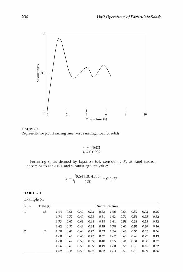
236 Unit Operations of Particulate Solids
s1 = 0.1603 s2 = 0.0992
Pertaining sr, as defined by Equation 6.4, considering XA as sand fraction according to Table 6.1, and substituting such value:
sr = =0 5415 0 4585120
0 0455. ( . )
.
Mixing time (h)
0
0.5
1.0M
ixin
g in
dex
2 4 6 8 100
Figure 6.1Representative plot of mixing time versus mixing index for solids.
Table 6.1
Example 6.1
Run Time (s) Sand Fraction
1 45 0.64 0.66 0.49 0.32 0.33 0.68 0.64 0.52 0.32 0.260.74 0.77 0.49 0.33 0.31 0.63 0.70 0.54 0.35 0.320.73 0.67 0.64 0.48 0.38 0.61 0.58 0.38 0.33 0.320.62 0.87 0.49 0.44 0.35 0.70 0.60 0.52 0.39 0.36
2 87 0.50 0.48 0.49 0.42 0.33 0.54 0.67 0.53 0.35 0.360.60 0.65 0.46 0.43 0.37 0.62 0.63 0.49 0.47 0.490.60 0.62 0.58 0.59 0.48 0.55 0.46 0.34 0.38 0.370.56 0.63 0.52 0.39 0.49 0.60 0.58 0.45 0.45 0.320.59 0.48 0.50 0.52 0.32 0.63 0.59 0.47 0.39 0.36

Mixing 237
Using, then, Equation 6.3 values of the mixing index M2 are calculated for each experimental run as
M
M
2 1
2 2
0 16030 0455
3 5321
0 09920 0455
2 1802
−
−
= =
= =
.
..
.
..
Using the corresponding values of the mixing index M2 calculated above, and substituting in Equation 6.8 for each experimental run:
k
k
1
2
145
1 1 120
1 1 3 52310 0053
187
1 1 120
1
=− −
=
=−
ln/
( / . ).
ln/
−−=
( / . ).
1 2 18020 0059
With average value of k = 0.0056 and the required optimum for the mixing index (1/M2) = 0.9, substituting again in Equation 6.8:
t = −−
=10 0056
1 0 09131 0 9
394 07.
..
.ln s
Consequently, an optimum mixing time would be 394 s, approximately.
example 6.2
In a mixing operation, 150 g wheat are blended with 250 g sorghum. Samples with an estimate number of 1500 particles are taken periodically to verify the progress of the operation. Calculate the optimum mixing time according to data reported in Table 6.2.
SoluTion
This example follows the same direction as the previous one. There is not a pre-established ideal mixing index to be attained in this case, however, and so the
Table 6.2
Example 6.2
Run Time (min) Wheat Fraction
1 1.0 0.52 0.56 0.38 0.33 0.59 0.48 0.28 0.22 0.62 0.60 0.68 0.51 0.55 0.54 0.30 0.33 0.50 0.28 0.38 0.53
2 1.5 0.44 0.47 0.55 0.50 0.51 0.40 0.41 0.46 0.55 0.60 0.58 0.55 0.67 0.63 0.50 0.69 0.49 0.51 0.60 0.67
3 2.0 0.50 0.53 0.48 0.45 0.54 0.47 0.55 0.50 0.40 0.42 0.51 0.44 0.41 0.41 0.42 0.57 0.43 0.42 0.50 0.51
238 Unit Operations of Particulate Solids
mixing index will be averaged just like the k value in Equation 6.8 will be also averaged from the experimental data given in Table 6.2. Therefore, using Equation 6.1, the three values for s from Table 6.2 are
s1 = 0.1343 s2 = 0.0855 s3 = 0.0529
The value of sr, considering XA the fraction of wheat as indicated in Table 6.2 is, thus
sr = =0 375 0 6251500
0 0125. ( . )
.
Mixing indices M2 corresponding to each experiment are then calculated from Equation 6.3 as
M
M
M
2 1
2 2
2 3
0 13430 0125
10 744
0 08550 0125
6 840
0 0529
−
−
−
= =
= =
=
.
..
.
..
.00 0125
4 232.
.=
Also, corresponding k values transposed from Equation 6.8 are
k
k
1
2
11
1 1 1500
1 1 10 7440 0715
11 5
1 1 1500
=− −
=
=−
ln
ln
/
/ ..
.
/ −
=
=− −
=
1 1 6 8400 0879
12
1 1 1500
1 1 4 23203
/ ..
ln/
/ .k ..1217
Using average values of k and M2 and substituting into the same Equation 6.8, an approximate mixing time is calculated as follows:
t =
− −
=10 0937
1 1 1500
1 17 2821 29
.
/
/ ..ln min
The calculated mixing time of about 1.3 min was obtained for an averaged 1/M2 value very low, that is (1/M2) ≈ 0.14, considering that the ideal value should approach unity. Since the estimates of k and mixing indices cannot be taken

Mixing 239
outside of the experimental data, the obvious conclusion is that experimental runs were all short in time, and more experimentation is needed at more pro-longed times. From the trend shown in determination of k and M2 values, it can be implied that an equilibrium mixing–segregation is far from being established within the reported times.
6.4 Mixing Equipment
In general terms, mixers for dry solids have nothing to do with mixers involving a liquid phase. According to the mixing mechanisms previously discussed, solids mixers can be classified into two groups: segregating mix-ers and nonsegregating mixers. The former operate mainly by a diffusive mechanism while the latter practically involve a convective mechanism. Segregating mixers are normally nonimpeller-type units, such as tumbler mixers, whereas nonsegregating mixers may include screws, blades and ploughs, in their designs, and examples of them include horizontal trough mixers and vertical screw mixers. Solids mixing can be carried out satis-factorily in equipment units serving other purposes in the materials processing industries. An example of this is the use of fluidized beds to perform solids mixing duties. Mixing times required in fluidized beds are significantly lower than those required in conventional powder mixers. Van Deemter (1985) discussed different mixing mechanisms prevailing in fluidized beds.
6.4.1 Tumbling Mixers
These mixing units operate by the principle of promoting blending by con-tact of masses of solids inside a revolving vessel. The vessels take various forms, such as those illustrated in Figure 6.2, and may be fitted with baffles or stays to improve their performance. The shells rotate at variable speeds (up to 100 rpm), and with working capacities around 50% to 60% of the total. They are manufactured using a wide variety of materials, including stain-less steel. This type of equipment is best suitable for gentle blending of powders with similar physical characteristics. Segregation can represent a problem if particles vary, particularly in size and shape. Rotation speed may be fixed between 50% and 80% of the critical rotation speed Ncr given by the following relationship:
N
Rcr
max
= 0 498.
(6.9)

240 Unit Operations of Particulate Solids
6.4.2 Horizontal Trough Mixers
Horizontal trough mixers consist of a semicylindrical horizontal vessel in which one or more rotating devices are located. For simple operations single or twin screw conveyors are appropriate and one passage through such a system may be good enough. For more demanding duties a ribbon mixer, like the one shown in Figure 6.3, may be used. A typical design of a ribbon mixer will consist of two counteracting ribbons mounted on the same shaft. One moves the solids slowly in one direction while the other moves it quickly in the opposite direction. There is a resultant movement of solids in one direction, and so the equipment can be used as a continuous mixer. Some other types of ribbon mixers operate on a batch basis. In these designs troughs may be closed, so as to minimize dust hazard, or may be jacketed to allow temperature control. Due to small clearance between the ribbon and the trough wall, this kind of mixers can cause particle damage and may consume high amounts of power.
(a)
(b)
(c)
(d)
Figure 6.2Tumbler mixers used in food powder blending: (a) horizontal cylinder, (b) double cone, (c) V-cone, and (d) Y-cone.

Mixing 241
6.4.3 Vertical Screw Mixers
In vertical screw mixers a rotating vertical screw is located in a cylindrical or cone-shaped vessel. The screw may be mounted centrally in the vessel or may rotate or orbit around the central axis of the vessel near the wall. Such mixers are schematically shown in Figure 6.4a and b, respectively. The latter arrangement is more effective and stagnant layers near the wall are elimi-nated. Vertical screw mixers are quick, efficient, and particularly useful for mixing small quantities of additives into large masses of material.
6.5 Design and Selection Factors
Before selecting solids-mixing equipment, a careful study ought to be made of several performance characteristics. As previously stated, mixing of
Feed
Product
Figure 6.3Plain view of an open ribbon mixer.
(a)
(b)
Figure 6.4Vertical screw mixers: (a) central screw and (b) orbiting screw.

242 Unit Operations of Particulate Solids
powdered solids is a complex operation and mathematical modeling can be hardly used. Many factors affect the operation of solids blending, and so process features such as mixing homogeneity and time, loading and discharging arrangements, power consumption, equipment wear, and so on need to be analyzed and properly weighed up in order to take the most convenient decision.
As has already been mentioned, blending uniformity and mixing rate are best evaluated using design graphs, bearing in mind the tendency to segre-gate and considering that long mixing times tend to worsen, rather than improving, efficiency. Solids mixing can be a batch or continuous operation. In batch mode, proper mixing design will produce the desired blend in few minutes. Determination of residence time in continuous operation is a more difficult task but, considering the main properties of solids blending, such times also tend to be short, in the order of few minutes or even seconds. The ribbon-type mixer is often used for continuous mixing, although it is also employed for batch mixing. Continuous mixing should be considered an option only if a single formulation can be run for an extended period, or when the fluctuations of the outgoing product are within process require-ments. When any of these factors are compromised, the batch mode of opera-tion would be preferred as to assure the most attainable mixing uniformity.
Loading and discharge are also important aspects, more critical in con-tinuous operation mode. The total handling system must be considered in order to obtain optimum charging and discharging conditions. This would include the efficient use of weight hoppers and surge bins, minor-ingredient premixing, location of discharge gates, and any other ancillary device used to aid the continuity of the process.
Power requirements are not a major concern when choosing solids mixers since other considerations usually predominate. Sufficient power must be provided in order to handle the maximum needs, as well as to prevent changes during the mixing operation. When materials and operating condi-tions are subjected to variation, enough power should be made available for the heaviest bulk-density materials and for the extreme conditions of opera-tion. If the loaded equipment is to be started from rest, there should be suf-ficient power for this. When speed variations may be desirable, this should be taken into account for power requirements planning.
The ease, frequency, and thoroughness of cleaning are crucial when batches of different nature are to be mixed alternatively in the same equipment. Plain tumbling vessels are easy to clean, provided that adequate openings are available. Areas which could be difficult to clean are seals or stuffing boxes, crevices at baffle support, any corners, and discharge arrangements. If clean-ing between different batches is time consuming, several small mixers should be considered instead of a large single unit.
Dust formation should be avoided for safety reasons and when loss of dust may significantly affect batch composition. When dust release to the sur-rounding atmosphere cannot be avoided, the use of solid–gas separation

Mixing 243
devices, such as cyclones or bag filters, should to be considered as part of the design. Minimization of dust formation can be achieved by using less dusty but equally satisfactory batch ingredients, by employing palletized forms of extremely dusty materials, by proper venting so as to enable filtering or dis-placed air rather than unregulated loss of dust-laden air, or by addition of liquids if tolerable. Water addition in small quantities would be effective in minimizing dust on discharge from the mixer, and it will also render the batch less dusty in subsequent handling stages. Water or any other liquid should be directed into the batch material instead of onto the bare surface of the mixer, since this could cause buildup. Spraying by using a nozzle would be the considered the most convenient way of incorporations moisture into the mixing batch. Nozzle spray pressure should be sufficient to penetrate the batch, but not so high as to cause heavy splashing. The liquid should be added to the well-mixed batch, particularly when premature addition of liq-uid could impair the adequacy of blending. Also, both time of addition and time of application are important and should be carefully considered. Quantity of added moisture should be carefully considered because an excessive amount may cause the solids being blended to deliver a product showing a paste-like consistency.
Equipment wear could be taken as a crucial issue especially with abrasive materials. Abrasion-resistant coatings, such as rubber coating, special alloys, or platings, need to be considered in these cases. Any internal agitator device may wear even when operating at slow speed. When high abrasive materials are to be mixed, the benefits of an agglomerated-breaking device must be weighed up against potential contamination and maintenance costs.
The capacity would be an important factor when the mixed batches vary considerably in size from time to time. There are some features of the mixing operation which are not flexible in terms of capacity. For example, certain agitation devices in tumbler mixers do not function properly unless a given capacity is kept. In general, the effect of percentage of mixer volume occu-pied by the batch on the adequacy of mixing should be considered when changing from recommended operating volumes are planned.
Dry powder mixers should be selected or designed for a particular opera-tion, firstly by analyzing and giving careful examinations to the applicable areas discussed above. Mixer selection should also involve consideration of the place of the mixer within the overall process. Possible integration of many steps within the overall processing of solids in a particular applica-tion deserves scrutiny at this time. If there is no machinery available including all the necessary requirements, consideration should be given to modifications in order to obtain the most desirable features combination of the equipment.
Pilot tests are relevant in the final decision of selection or design of any specific mixing process. In general larger pilot plant units would provide more reliable data for performance prediction of large-scale powder mixing plants. With geometrically similar tumblers, if the speeds are adjusted to

244 Unit Operations of Particulate Solids
give comparable motion and the mixer volume fraction occupied by the load is the same, scale-up of results will be straightforward. The presence of inter-nal rotating devices leads to difficulties in scaling-up clearances, blade area to mixture volume, and sizes as well as speeds of the rotating devices. The actual materials to be processes in the industrial operation should be used if possible in the scale-up procedure. If substitute materials need to be used, they should have the same mixing characteristics. Differences in materials of construction between the pilot and the production unit should be consid-ered, since these may have a bearing on caking, abrasion, and some other adverse effects.
6.6 Laboratory Exercise: Determination of Blending Indices for Different Tumbling Mixers
6.6.1 introduction
Solid–solid mixing processes normally start by pouring known quantities or two or more solids into a mixing unit. The overall proportion of any compo-nent is known by the relation between the mass of that component and the total mass of all components (i.e., the solids fraction). If two components are mixed in equal proportion, it would be expected that uniformity of mixing can be verified by sampling, and when all extracted samples present propor-tions of 0.5 for any of the components, a perfect mixing had been achieved. It is unrealistic, however, to expect all the samples to have an exact proportion of one component: some samples will have more, some less, but the overall mean average of one component as proportion, would tend to equal the orig-inal proportion due to the solids fractions combined initially. Most of the proposed models to determined mixing indices as an indicative of blending homogeneity are based on experimental determination of sample’s mean values and variances. The objective of the experiment is to determine mix-ing indices for a solids mixing operation using two types of tumbling equipment.
6.6.2 equipment and Materials
Two tumbling mixers (e.g., double cone mixer and V-cone mixer). Two batches of differently colored ballotini beads with a size range 0.8–1.2 mm each and the same density.
6.6.3 instruments or apparatuses
Set of standard sieves and sieve shaker as well as analytical balance.

Mixing 245
6.6.4 operation of the Mixers
Standardize the size of each solid sample by using a 1 mm sieve, as •to separate the fine fraction of Sample A and the coarse fraction of Sample B.Adjust the speed of rotation of one of the mixers.•Weight the same quantity of each standardized solid, for example, •500 g, and pour them into the mixer.Start the mixing operation at constant speed and record the time •(t = 0 min).Stop the mixer after two minutes (• t = 2 min).Collect five 30 g spot samples from different parts of the mixer.•Measure and record the weights.•Sieve them using the 1 mm screen and collect the fine and coarse •fractions of the sample.Record the weights of the fractions separated in the previous step.•Make an estimate of the number of particles in the sample, either by •counting (using the bear eye or a microscope) or relating properties like minimum weight detected with particles able to be counted.Continue the mixing operation for 2 more minutes and stop at this •third time (t = 4 min). Repeat the procedure for the t = 2 min sample.Continue, progressively, taking samples and repeating procedures •up to complete 10 min mixing.Repeat the experiment for the second mixer.•
6.6.5 Calculations and report
The recorded weight of the fractions separated from the spot sam-•ples will give an estimate of the proportion of one selected compo-nent. By determining these proportions, elaborate a table such as Tables 6.1 or 6.2.With the estimate of the number of particles in the spot samples, •make a development like the one given in the solution of Examples 6.1 and 6.2. Calculate values of k using Equation 6.8.Elaborate plots like the one shown in Figure 6.1 for both tumbling •methods.Recalculate an ideal time for the two tested processes, to reach a •value of 1/M2 of 0.95.Present a complete written report, according to scientific report •guidelines, either given by instructor or consulted in the literature.
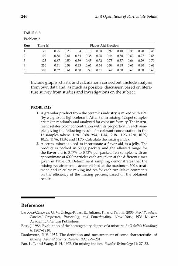
246 Unit Operations of Particulate Solids
Include graphs, charts, and calculations carried out. Include analysis from own data and, as much as possible, discussion based on litera-ture survey from studies and investigations on the subject.
PROBLEMS
1. A granular product from the ceramics industry is mixed with 12% (by weight) of a light colorant. After 3 min mixing, 12 spot samples are taken randomly and analyzed for color uniformity. The instru-ment relates color concentration with its proportion in each sam-ple, giving the following results for colorant concentration in the 12 samples taken: 11.28, 10.88, 9.94, 11.34, 12.18, 11.23, 12.91, 10.92, 10.22, 11.96, 11.87, and 11.75. Calculate the mixing index.
2. A screw mixer is used to incorporate a flavor aid to a jelly. The product is packed in 500 g packets and the allowed range for the flavor aid is 0.57% to 0.63% per packet. Ten samples with an approximate of 6000 particles each are taken at the different times given in Table 6.3. Determine if sampling demonstrates that the mixing requirement is accomplished at the maximum 500 s treat-ment, and calculate mixing indices for each run. Make comments on the efficiency of the mixing process, based on the obtained results.
References
Barbosa-Cánovas, G. V., Ortega-Rivas, E., Juliano, P., and Yan, H. 2005. Food Powders: Physical Properties, Processing, and Functionality. New York, NY: Kluwer Academic/Plenum Publishers.
Boss, J. 1986. Evaluation of the homogeneity degree of a mixture. Bulk Solids Handling 6: 1207–1210.
Dankwertz, P. V. 1952. The definition and measurement of some characteristics of mixing. Applied Science Research 3A: 279–281.
Fan, L. T. and Wang, R. H. 1975. On mixing indices. Powder Technology 11: 27–32.
Table 6.3
Problem 2
Run Time (s) Flavor Aid Fraction
1 75 0.95 0.25 1.04 0.15 0.88 0.92 0.18 0.35 0.20 0.482 100 0.58 0.81 0.84 0.38 0.78 0.46 0.50 0.60 0.27 0.683 125 0.67 0.50 0.59 0.45 0.72 0.75 0.57 0.66 0.29 0.704 250 0.61 0.58 0.63 0.62 0.54 0.59 0.68 0.62 0.60 0.635 500 0.62 0.61 0.60 0.59 0.61 0.62 0.60 0.60 0.58 0.60

Mixing 247
Harnby, N. 1985. The selection of powder mixers. In Mixing in the Process Industries, Harnby, N., Edwards, M. F., and Nienow, A. W. (eds.). London: Butterworths.
Lacey, P. M. C. 1954. Developments on the theory of particle mixing. Journal of Applied Chemistry 4: 257–268.
McCabe, W. L., Smith, J. C., and Harriot, P. 2005. Unit Operations in Chemical Engineering, 7th Ed. New York, NY: McGraw-Hill.
Niranjan, K. 1995. An appraisal of the characteristics of food mixing. In Food Process Design and Evaluation, Singh, R. K. (ed.). Lancaster, PA, USA: Technomics.
Niranjan, K. and de Alwis, A. A. 1993. Agitation and agitator design. In: Encyclopedia of Food Science, Food Technology and Nutrition, Vol. 1, Macrae, R., Robinson, R. K. and Sadler, M. (eds.). London: Academic Press.
Poole, K. R., Taylor, R. F., and Wall, G. P. 1964. Mixing powders to fine scale homoge-neity: studies of batch mixing. Transactions of the Institution of Chemical Engineers 42: T305–T315.
Stange, K. 1963. Die mischgute einer Zufallsmischung aus drei und mehr Komponenten. Chemie Ingenieur Techik 35: 580–582.
Van Deemter, J. J. 1985. Mixing. In Fluidization, 2nd Ed. Davidson, J. F., Clift, R. and Harrison, D. (eds.). London: Academic Press.
Williams, J. C. 1968/1969. The mixing of dry powders. Powder Technology 2: 13–20.


249
7Fluidization
7.1 Theoretical Fundamentals
Particulate solids, when packed within a container, form an arrangement allowing for the void space between particles to be filled by a gas, normally air. Such arrangement has generally been referred to as a bed, and the inter-actions between the solids particles and the voids filled with air are related by an important property known as porosity. Any particular fluid flowing at low velocities through a porous bed of solid particles, for example, in a packed tower, does not cause the particles to move. The fluid passes through the small, tortuous channels, losing pressure energy. The pressure drop in a stationary bed of solids can be described by fundamental fluid mechanics theory. However, if the fluid velocity is steadily increased a point is eventu-ally reached at which the particles no longer remain stationary but are fluid-ized under the influence of the fluid. Fluidization is a relevant property of particulate solids since, when fluidized, particulate solids within a fluid stream could behave somewhat as fluids and, therefore, they may be studied under the scope of fluid mechanics. Some fluid-like properties that fluidized bed present are, for example:
The surface of the bed becomes horizontal and, if disturbed, returns •quickly to horizontal.Like in a liquid, the pressure increases with depth.•Objects of lower density float on the surface of the fluidized bed, •whereas objects of higher density sink to the bottom of the fluidized bed.If a hole is opened on the wall of the containing vessel of the fluid-•ized bed, particles will pour out as a jet, similar to water from a puncture in a water container.Bubbles can rise through the fluidized bed and burst in the surface •as in a liquid. Moreover, the bubble shapes and rise velocities are similar to those of bubbles in liquids.

250 Unit Operations of Particulate Solids
The state of being fluidized, called “fluidization” as already done, turns out to be advantageous in numerous operations of the materials processing industry run, normally, by practicing chemical engineers.
7.1.1 bulk Density and Porosity of beds
When a powder just fills a vessel of known volume V and the mass of the powder is m then the bulk density of the powder is m/V. However, if the ves-sel is tapped in most cases the powder will settle leaving top empty space, so adding more powder would be necessary to end with the vessel completely filled. If the mass now filling the vessel is m′ then the bulk density is m′/V > m/V. Clearly, this change in density just described has been caused by the influence of the fraction of volume not occupied by a particle, known as porosity. The bulk density is, therefore, the mass of particles that occupies a unit volume of a bed, while porosity or voidage is defined as the volume of the voids within the bed divided by the total volume of the bed. These two properties are in fact related via the particle density in that, for a unit volume of the bulk powder, there must be the following mass balance:
ρ ρ ε ρ εb s a= − +( )1 (7.1)
where ρb is the powder bulk density, ρs is the particle density, ε is the porosity, and ρa is the air density. As the air density is small relative to the powder density, it can be neglected and the porosity can thus be calculated simply as
ε ρ ρ
ρ= −( )s b
s (7.2)
Equation 7.2 gives the porosity or voidage of the powder and whether or not this includes the pores within the particles depends on the definition of par-ticle density used in such evaluation.
7.1.2 Fluid Flow through Solids beds
Fluidization can be considered a special case of fluid–solids flow with a rather complex behavior (Jackson, 2000). The fluid flow resistance through the voids in a bed of solids is the resultant of the total drag of all the particles in the bed (McCabe et al., 2005). Depending on the particle’s Reynolds num-ber, laminar flow, turbulent flow, form drag, separation, and wake formation may occur. Similar to the drag of a single solid particle, there is no sharp transition between laminar and turbulent flow like that occurring in flow through conduits of constant cross section. Calculations of the total pressure drop through a bed of solids can be based on estimates of the total drag of the fluid on the solid boundaries of the tortuous channels through the bed of

Fluidization 251
particles (Zenz and Othmer, 1960). This can be done by assuming that the actual channels may be effectively replaced by a set of identical parallel con-duits, each of variable cross section, and that the mean hydraulic radius of the channels is appropriate to account for the variations in channel cross-sectional size and shape. The total drag per unit area of channel wall would be the sum of viscous drag forces and inertial forces, while a direct determi-nation of the total surface area of the bed would be the sum of the individual surface area of all particles within the bed. Since this latter approach would be unpractical and unattainable, total surface area could be derived from estimation of the relation surface volume for the solids in the bed. The vol-ume fraction of solids particles in a bed can be defined as 1–ε, being ε the porosity previously defined by Equation 7.2. The bed porosity can easily evaluated in situ by filling the bed with a liquid, draining, and comparing the volume of the liquid to the total volume of the bed as calculated from its depth and cross section.
The volumetric average velocity of the fluid through the channels within the bed u and the velocity of the fluid stream just before entering to the first layer of solids u0 are related by the porosity. The usual configuration of a packed bed is a large cylindrical vessel with a supporting grid some distance above the bottom of the tower. The velocity u0 is known as the superficial velocity or empty-tower velocity, and u is the upward or downward velocity in the open section below the grid or in the empty tower above the bed. The average free cross section of all the channels has the same ratio to the total cross section of the empty tower, while the volume of the channels has the same ratio to the total volume of the bed of solids. The above-mentioned rela-tion between u and u0 can be represented by
u
u= 0
ε (7.3)
7.1.3 Mechanism of Fluidization: aggregative and Particulate
The effect of flowing of a fluid through a bed of particles may cause three effects as a function of the fluid velocity: the bed may expand a little but remain fixed at lower fluid velocities, the particles may become freely sup-ported in the fluid al higher velocities, and the particles may become totally suspended by the fluid stream and may be transported within it as in pneu-matic transport. If the fluid flow rate is increased above the minimum required to produce a fluidized bed, this will continue to expand so that the average distance between particles will become greater, or the fluid excess will pass through the bed in the form of rising pockets of gas giving origin essentially to a two-phase system. From the earliest applications of fluidized beds it was noticed that liquid-fluidized beds presented a smooth appear-ance expending progressively as the fluid flow rate increased, while most

252 Unit Operations of Particulate Solids
gas-fluidized beds were typically heterogeneous containing the rising pock-ets of gas previously mentioned practically free from particles. These gas pockets were referred to as “bubbles” and the terms “particulate” and “aggregative” were introduced to describe the two types of fluidized behav-ior. Generally, particulate fluidization occurs with solid–liquid systems and with solid–gas systems when the particles are very fine and only over a lim-ited range of velocities. Aggregative fluidization occurs with all other solid–gas systems and, sometimes, with solid–liquid systems for high-density solids. The growth rate of a small bubble will generally be greater in solid–gas systems that in solid–liquid systems.
The type of fluidization occurring in a process will be related to the maxi-mum stable size of bubble that can exist within the fluidized bed. If the cir-culation velocity of gas within the bubble exceeds the terminal velocity of particles, these will be sucked in at the rear of the bubble, which will thus tend to be destroyed. Since the bubble rise velocity will increase with bubble volume, being substantially independent of the properties of the fluidized bed, the maximum stable bubble size will increase with the terminal falling velocity of the particles in the fluid. If this size exceeds by a large amount compared to the particle diameter, the bubble will appear obvious and the fluidization will be aggregative. On the other hand, when the bubble size is of the same order of the particle diameter, such bubble can no longer be dis-tinguished from the interstitial gas and the fluidization will appear to be particulate. On this basis, most solid–gas systems will give rise to aggrega-tive fluidization whereas most solid–liquid systems will originate particu-late fluidization.
An empirical criterion to distinguish the type of fluidization governing a process was proposed quite early by Wilhelm and Kwauk (1948). They sug-gested the use of the Froude number, that is (Fr mf= u xg2 / ) as the criterion for the type of fluidization observed. In general, aggregative fluidization occurs at values above unit and particulate fluidization at values below unity. In the Froude number umf denotes the minimum fluidization velocity and x a parti-cle equivalent diameter. Within the context of qualitative distinctions between particulate and aggregative fluidization, research efforts have been focused for a while into three avenues. One has consisted of lengthy mathematical analyses in which the bed has been treated as a homogeneous mass regard-less of its physical details. A second one has sought empirical correlations of associated heat and mass transfer, as well as bed expansion and other proper-ties necessary in equipment design. The third avenue has directed research in studying the lack homogeneities occurring in the more widely applicable aggregatively or gas-fluidized beds, that is, investigating fundamentally the bubble formation process from experimental and hydrodynamic viewpoints. The first of these directions was to distinguish between gas- and liquid-fluid-ized beds; the second provided necessary data sufficient for first-generation plant designs; and the third produced basic data on bubble shape, velocity of rise, effect on particle mixing, and related observations.

Fluidization 253
7.2 Fluidized Regimes
An understanding of the fluidized regimes within the bed should include criteria to distinguish the limits from the fixed to the fluidized, and to the suspended (transport) state of particles in a stream of fluid. The relation between the superficial velocity u of the fluid, calculated from the whole cross section of the containing vessel, and the pressure gradient is shown in Figure 7.1. If the flow is streamline a straight line of slope unity is obtained at low velocities. At the fluidizing point the pressure gradient begins to fall because the porosity of the bed increases, and the fall continues until the velocity is sufficient for transport of the solids to take place. The pressure gradient then starts to increase again because the frictional drag of the fluid at the walls of the tube starts to become significant. A minimum fluidizing velocity will mark a transition from the fixed to the fluidized state. At the minimum fluid-izing velocity it may be expected that flow relations for the fixed bed would be applicable to the fluidized bed. At the opposite limit when a bed is fully expanded so that its voidage approaches unity, it consists effectively of single isolated particles suspended in the fluid, and thus any relationship describ-ing a fluidized bed should extrapolate at unit voidage to one applicable to an individual particle. At intermediate conditions, the particulate fluidized bed is hydrodynamically similar to a sedimenting suspension.
In a fluidized bed the particles undergo no net movement as they are sup-ported by the upward fluid flow, whereas in a sedimenting suspension the particles are moving continuously downward and the only net movement of
Fixedbed
Fluidizedbed
Transport
Log u
Log
(ΔP B)
/H
Figure 7.1Pressure gradient in bed as a function of fluid velocity.
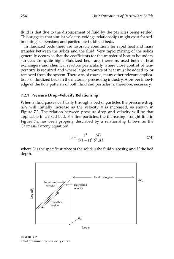
254 Unit Operations of Particulate Solids
fluid is that due to the displacement of fluid by the particles being settled. This suggests that similar velocity–voidage relationships might exist for sed-imenting suspensions and particulate-fluidized beds.
In fluidized beds there are favorable conditions for rapid heat and mass transfer between the solids and the fluid. Very rapid mixing of the solids generally occurs so that the coefficients for the transfer of heat to boundary surfaces are quite high. Fluidized beds are, therefore, used both as heat exchangers and chemical reactors particularly where close control of tem-perature is required and where large amounts of heat must be added to, or removed from the system. There are, of course, many other relevant applica-tions of fluidized beds in the materials processing industry. A proper knowl-edge of the flow patterns of both fluid and particles is, therefore, necessary.
7.2.1 Pressure Drop–Velocity relationship
When a fluid passes vertically through a bed of particles the pressure drop ΔPB will initially increase as the velocity u is increased, as shown in Figure 7.2. The relation between pressure drop and velocity will be that applicable to a fixed bed. For fine particles, the increasing straight line in Figure 7.2 has been properly described by a relationship known as the Carman–Kozeny equation:
u
PS H
=−ε
ε µ
3
2B
5(1 )∆2
(7.4)
where S is the specific surface of the solid, μ the fluid viscosity, and H the bed depth.
Fluidized region
Fixed bedregion
Increasingvelocity Decreasing
velocity
umf
Log u
ΔPeq
Log ΔP
B
Figure 7.2Ideal pressure drop–velocity curve.

Fluidization 255
As the velocity reaches a point in which the frictional pressure drop equals the buoyant weight per unit area of particles (ΔPeq), any further increase in velocity must result in a slight upward movement of the particles forming the bed. The particles will rearrange so that the resistance to fluid flow will decrease and, in general, the voidage of the bed will increase. In an idealized system, the pressure drop ΔPeq will remain constant, as represented by the plateau in Figure 7.2. Further increases in velocity will result in continuing expansion of the bed until, eventually, any further separation of the particles will only be possible if they become physically separated from one another and become free to move within the fluid. At this stage the bed is just fluid-ized, is said to be at the “point of incipient fluidization,” and the superficial fluid velocity there is known as the “minimum fluidizing velocity” umf. If the fluid velocity is further increased the pressure drop over the bed remains constant, but if the fluid velocity is progressively reduced the pressure remains constant at the point of incipient fluidization. Further reduction of velocity is accompanied by a progressive decrease in pressure drop and the pressure drop–velocity curve will generally be lower than the one obtained while the velocity was being increased, since in the absence of vibration the bed voidage will remain approximately at the value εmf corresponding to a bed at the point of incipient fluidization.
The behavior described above is an idealized one and the deviation from it, gives a good indication of the factors influencing the performance of the bed. Deviations from ideal behavior can be due to a number of reasons. For example, as the velocity approaches the minimum fluidizing velocity some normal expansion will occur before the pressure drop has reached the buoy-ant weight per unit area of bed. This effect would be most marked when the bed is initially highly consolidated. In addition, local variations in the per-meability of a randomly packed bed would tend to cause a gradual transition between the two sections of the curve. Also, the tendency of the particles to interlock with one another may cause partial bridging, particularly in small-diameter beds, with the results that frictional forces are exerted by the walls of the bed container. It is, therefore, possible for pressure drops in excess of the theoretical value to be obtained, so that the curve will pass through a point of maximum pressure drop, exhibiting a small characteristic “hump,” as shown in Figure 7.3. Furthermore, nonuniformity in the structure of the bed will result in preferential flow of fluid in particular areas, resulting in possible coexistence of fixed and fluidized regions within the bed. The bed may appear to be well fluidized, but part of its weight may still be borne by the bed distributor, resulting in a pressure drop below its expected value. The minimum velocity at which the bed weight is fully supported by the fluid appears as point ufs in Figure 7.4.
The form of the curve of pressure drop against velocity for the fixed and fluidized beds should provide considerable amount of information on the structure of the bed. Deviations from the idealized behavior are attributable to intraparticle forces and maldistribution of the fluid in the bed. For practical

256 Unit Operations of Particulate Solids
purposes, the minimum fluidized velocity is defined as shown in Figure 7.4 as the point of intersection of the pressure drop lines for the fixed and fluid-ized regimes.
7.2.2 incipient Fluidization and Minimum Fluidizing Velocity
Due to the complexity of interaction of fluid–solid systems is not possible to predict precisely the behavior of fluidized-bed operations. With solid–gas
Log u
ΔPeq
Log ΔP
B
Figure 7.3Pressure drop over fixed and fluidized beds as a function of fluid velocity.
Log u
umf ufs
Log ΔP
B
Figure 7.4Effect of presence of nonfluidized regions in bed.

Fluidization 257
systems there is a very marked contrast in the behavior of solid materials: some of them will fluidize extremely well, while some others will be virtually incapable of being fluidized. The following properties of the solid and the fluid will be determinant in achieving well-fluidized systems: (a) low particle den-sity, (b) small particle size, (c) small particle size range, (d) particle shape approaching spherical, and (e) high fluid density. The properties of the solids identified as the more influential in making it capable of giving a well-fluid-ized system are small particle size and low density. Unfortunately, those same properties have been observed to make the initiation of fluidization difficult. If surface forces between the particles are significant, they will be greater with small particles because of their high specific surface. If the particles possess low density, the gravitational forces tending to pull them apart will be small. Thus, small low-density particles can cause serious channeling even though they may fluidize pretty well once they have been brought into suspension.
In an idealized system the minimum fluidizing velocity is that at which the bed suddenly changes from a fixed to a fluidized state. In practice, how-ever, there may be a large transitional region so that the minimum fluidizing velocity will be difficult to determine. The problem of definition generally becomes greater for particles of a wide size range. The minimum fluidized velocity can be determined graphically or can be calculated analytically. In the graphical method, that determination can be conveniently done by using the plot of frictional pressure drop against velocity. If separate lines are drawn through the points for the fixed and fluidized regions, and the points in the intermediate region are ignored, the point of intersection of these two lines will give a reproducible value for the minimum fluidized velocity, just as shown in Figure 7.4.
An approximate analytical calculation of the minimum fluidizing velocity can be carried out by using an expression for the relation between pressure drop and superficial velocity for a fixed bed and putting the pressure drop equal to the buoyant weight of the particles. The pressure drop through the bed is then equal to its apparent weight per unit area, and the porosity at the onset of fluidization is the maximum that the fixed bed can attain. Previous knowledge of the voidage of the bed at the minimum fluidizing velocity (εmf) would be necessary, but this would depend on the shape and size range of the particles. A value of about 0.4 would be appropriate for approximately spherical particles. Taking into account the above considerations, an expres-sion for the pressure drop over the fluidized bed at incipient fluidization will be given by
∆PB s f= = − −
mgA
Hg( )( )ρ ρ ε1
(7.5)
where m is the mass of solids in the bed, g is the acceleration due to gravity, A is the cross-sectional area of the bed, ρs is the solids density, and ρf is the fluid density.

258 Unit Operations of Particulate Solids
If the bed expands the product (1 – ε) will remain constant. Using the val-ues of each term proper for the conditions of incipient fluidization:
∆P H gB s f mf mf= − −( )( )ρ ρ ε1 (7.6)
For fine particles the pressure drop–velocity relationship will be given by the Carman–Kozeny equation, which will take the following form for incipi-ent fluidization:
u
PS Hmf
mf3
mf
B
mf=
−ε
ε µ5 1 2 2( )∆
(7.7)
Substituting Equation 7.6 into Equation 7.7, the following expression results:
u
gSmf
mf3
mf
s f= −−ε
ερ ρ
µ5 1 2( )( )
(7.8)
For uniform spherical particles S = 6/x, where x is an equivalent particle diameter. Also, taking εmf = 0.4, Equation 7.8 would transform into
u
x gmf
s f=−
0 000592
.( )ρ ρ
µ (7.9)
For larger particles, a more general equation such as the Blake, Carman, or Ergun (1952) equation must be used for the pressure drop through the fixed bed. Using the Ergun equation:
∆PB
mf
mf
mf3
mf mf
mf3
f mf2
Hux
ux
= − + −150
11 75
12
2
( ).
( )εε
µ εε
ρ
(7.10)
Substituting for ΔPB/Hmf from Equation 7.6 and multiplying both sides by ρfx3/μ2(1 – εmf), the following expression will result:
ρ ρ ρµ
εε
ρµ
ρµ
f s f mf
mf3
mf f
mf3
mf f( ) .−= − +
gx u x u x3
2
2
1501 1 75
ε (7.11)
Identifying the following groups:
ρ ρ ρµ
ρµ
f s f mf fmfGa and
( )Re
−= =
gx u x3
2
where Ga is the Galileo number and Remf is the Reynolds number at incipient fluidization point.
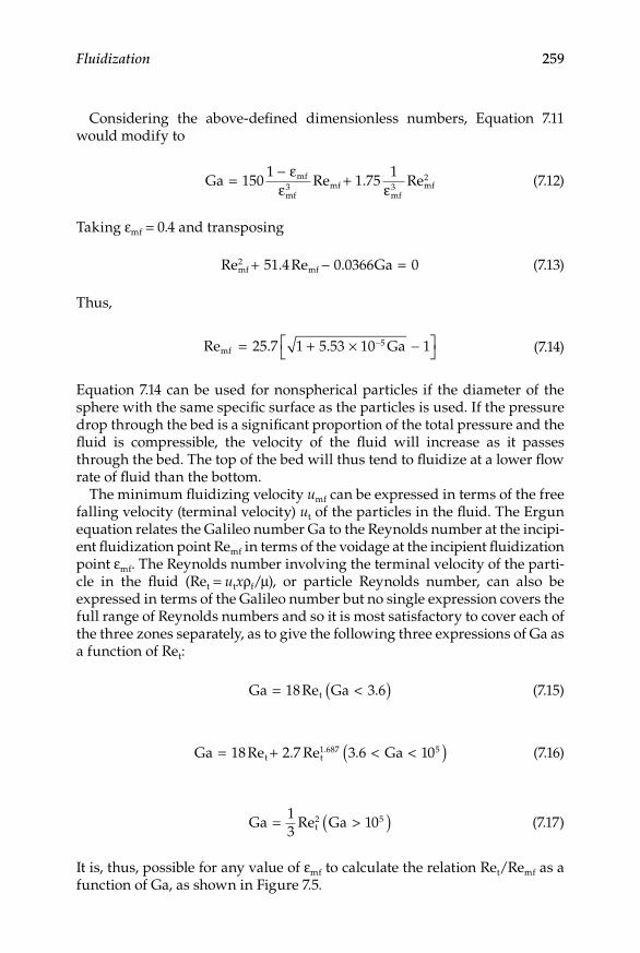
Fluidization 259
Considering the above-defined dimensionless numbers, Equation 7.11 would modify to
Ga mf
mf3 mf
mf3 mf= − +150
11 75
1 2εε ε
Re . Re
(7.12)
Taking εmf = 0.4 and transposing
Re . Re .mf2
mf Ga+ − =51 4 0 0366 0 (7.13)
Thus,
Re . .mf Ga= + × −
−25 7 1 5 53 10 15
(7.14)
Equation 7.14 can be used for nonspherical particles if the diameter of the sphere with the same specific surface as the particles is used. If the pressure drop through the bed is a significant proportion of the total pressure and the fluid is compressible, the velocity of the fluid will increase as it passes through the bed. The top of the bed will thus tend to fluidize at a lower flow rate of fluid than the bottom.
The minimum fluidizing velocity umf can be expressed in terms of the free falling velocity (terminal velocity) ut of the particles in the fluid. The Ergun equation relates the Galileo number Ga to the Reynolds number at the incipi-ent fluidization point Remf in terms of the voidage at the incipient fluidization point εmf. The Reynolds number involving the terminal velocity of the parti-cle in the fluid (Ret = utxρf/μ), or particle Reynolds number, can also be expressed in terms of the Galileo number but no single expression covers the full range of Reynolds numbers and so it is most satisfactory to cover each of the three zones separately, as to give the following three expressions of Ga as a function of Ret:
Ga Ga 3 6t= <( )18Re . (7.15)
Ga 3 6 Ga 1t t1.687 5= + < <( )18 2 7 0Re . Re . (7.16)
Ga Ga 1t
5= >( )13
02Re
(7.17)
It is, thus, possible for any value of εmf to calculate the relation Ret/Remf as a function of Ga, as shown in Figure 7.5.

260 Unit Operations of Particulate Solids
example 7.1
A bed of fractioned pulverized coal 65-mesh (Tyler) is fluidized by air at room-temperature conditions. The height of the static bed is 1.80 m. If the coal particles may be considered spherical, while their density is 1350 kg/m3, calculate the pres-sure drop required for fluidization.
SoluTion
Consulting a Tyler Standard Screen Scale Table, it can be read the value of the screen equivalent diameter as 0.208 mm, so the pulverized coal may be consid-ered a fine powder. Since the particles are taken as spherical, the ideal porosity ε = 0.4 can be used for calculation. Finally, from any reference book (or appendix of some engineering textbook) listing physical properties of materials, at approxi-mately 25°C the density of air is of the order of 1.2 kg/m3. Substituting directly into Equation 7.5:
∆PB2(1350 1.2)(1 0.4)(1.8)(9.81) 14,29 26 N m 14 3 kPa= − − = ≈0. / .
example 7.2
A bed of 100 kg dried peas is to be fluidized in chilled air at –5°C as a part of a process. The peas are 5 mm in size and their density approaches 1000 kg/m3.
10
20
30
40
50
60
70
80
90
100
110
10710610510410310210110010–110–20
εmf = 0.38
εmf = 0.40
εmf = 0.42
Ga: Galileo number
u t/u
mf o
r Re t
/Re m
f
Figure 7.5Ratio of terminal falling to minimum fluidization velocity as a function of Galileo number.
Fluidization 261
Calculate the air velocity, the pressure drop through the bed if the cross-sectional area is 0.3 m2, and the bed height at a voidage 20% above the minimum.
SoluTion
The peas can be considered spherical and homogeneous in size. The ideal void-age ε = 0.4, can therefore, be used. Consulting any reference book (or appendix of some engineering textbook) listing physical properties of materials, at approxi-mately –5°C the density of air is in the order of 1.3 kg/m3 while its viscosity is around 1.6 × 10⁻⁵ Pa s. The particulates are, obviously, large and so, the minimum fluidization velocity should be transposed from the expression of Refm in Equation 7.14:
ux
mf
g
f
Ga=
=
25 7 1 5 53 10 1
25 7 1 6 10 1 5 53 1
5
5
. ( ) .
. ( . .
µ
ρ
+ × −
× + ×
−
− 00 1
0 0051 3
5− −
Ga
. ( . )umf = 0.9692 m/s ≈ 1 m/s.
The pressure drop through the bed can be estimated substituting directly into the first right-hand term of Equation 7.5, that is;
∆PB 327 Pa= ( )( . )
.100 9 81
0 30=
The porosity at 20% above the minimum would be 0.48 and, thus, transposing for the height Hmf in Equation 7.6:
Hmf 64186m 64 m=
− −= ≈3270
1 0 48 1000 1 3 9 810 0
( . )( . )( . ). .
7.2.3 Heterogeneous Fluidization: bubbling
Bubbles or particle-free voids may appear in a fluidized bed once the mini-mum fluidization velocity has been surpassed. Bubbles in a gas-fluidized bed migrate upward, just like bubbles in a boiling liquid. Figure 7.6 shows the typical pattern followed by bubbles in many cases of fine particulate sol-ids fluidized by a gas. At superficial velocities above umf, fluidization may be either bubbling or nonbubbling. Some combinations of fluid and particles give rise to “only bubbling fluidization” while some other combinations give origin to “only non-bubbling fluidization.” Gas-fluidized systems will pres-ent only bubbling fluidization or nonbubbling fluidization starting at umf, followed by bubble fluidization as fluidizing velocity increases. Nonbubbling fluidization is also known as particulate or homogeneous fluidization,

262 Unit Operations of Particulate Solids
whereas bubbling fluidization is often referred to as aggregative or heteroge-neous fluidization.
The fluidization properties of a powder in air may be predicted by estab-lishing in which group of the Geldart’s classification (Chapter 2, Section 2.2.2) such powder lies. Since the range of gas velocities over which nonbubbling fluidization occurs in Group A powders is small, bubbling fluidization is the most commonly observed type in gas fluidized systems commercially in use. The superficial gas velocity at which bubbles first appear in a fluidized bed is known as the minimum bubbling velocity umb. Abrahamsen and Geldart (1980) correlated the maximum values of umb with gas and particle properties using the following equation:
u
xmb
F ge=
2 07 0 7160 06
0 347. ( ) ..
.
ρµ
(7.18)
where F is the fraction of powder less than 45 μm.In most solid–gas systems bubbling occurs when the gas velocity is
increased well over the minimum fluidizing velocity. The simplest descrip-tion of the expansion of a gas-fluidized bed comes from the two-phase the-ory of fluidization (Rhodes, 1998), originally attributed to Toomey and Johnstone (1952). This theory suggests that the bubbling fluidized bed is composed of two phases: the bubbling phase and the particulate phase (also known as the emulsion phase), and that all the gas in excess of that required to fluidize the system will pass through the bed in the form of bubbles.
The lower and upper limits of gas velocity at which a uniform particulate phase can exist are the minimum fluidizing velocity and the minimum bub-bling velocity, respectively. It is quite difficult to define the latter precisely, since it will depend critically on the previous history of the bed, on the nature
Coalescence
Eruption fromsurface
Rising ofbubbles
Bubbles reachingsurface and bursting
Figure 7.6Behavior of bubbles for a typical fluidized Group B powder (Geldart’s classification).

Fluidization 263
of the gas distributor, and on the presence of obstructions within the bed. The ratio umb/umf does give a measure of the degree to which the bed can be expanded, tending to be relatively high for fine low-density solids and high-density gas. There is a minimum stable size of bubbles that can exist within the particulate phase. Smaller bubbles tend to shrink and become assimi-lated in the dense phase, while large bubbles tend to grow at the expense of the gas in the continuous phase. If a bubble larger than the critical size is injected into an expanded bed, this will initially expand by an amount equal to the volume of injected gas. However, when the bubble breaks the surface, the bed level will fall back to a value below that before injection was effected. The transference of gas between dense and bubble phases within a fluidized bed is an important factor, which must be considered in designing fluidized beds as reactors.
Powders of small particle size and low density are difficult to fluidize ini-tially, but once they reach the fluidized state they can give origin to beds that can be expanded over a wide range before bubbling occurs. The formation of large bubbles in gas-fluidized systems is often prevented by introducing standard tower packings into the bed to produce what is known as a packed-fluidized bed.
The bed expansion can be expressed in terms of the fraction occupied by bubbles εB:
εB
mf mf
B
mf
B= − = − = −H H
HQ Q
Auu u
u (7.19)
where H is the bed depth at u and Hmf is the bed depth at umf; Q is the actual gas flow rate to the fluid bed and Qmf is the gas flow rate at incipient fluidi-zation; A is the bed section area; uB is the mean rise velocity of a bubble in the bed.
The voidage of the emulsion phase is taken to be that at minimum fluidiza-tion εmf. The mean bed voidage is then given by
( ) ( )( )1 1 1− = − −ε ε εB mf (7.20)
In practice, however, the two-phase flow theory overestimates the volume of gas passing through the bed as bubbles, that is, the visible bubble flow rate (Rhodes, 1998) and better estimates of bed expansion may be obtained by replacing (Q – Qmf) in Equation 7.19 with the following relationship for the bubble flow rate:
Q YA u uB mf= −( ) (7.21)
where: 0.8 < Y < 1.0 for Group A powders (Geldart’s classification) 0.6 < Y < 0.8 for Group B powders (Geldart’s classification) 0.2 < Y < 0.6 for Group D powders (Geldart’s classification)

264 Unit Operations of Particulate Solids
Strictly, the above equations should be written in terms of umb rather than umf, and Qmb rather than Qmf, so that they are valid for both Group A and Group B powders. Practically, however, it makes little difference, since both umb and umf are usually much smaller than the superficial fluidizing velocity u and, therefore: (u – umf) ≈ (u – umb).
7.2.4 Spouted beds
The spouted bed is a variant of the fluidized bed in which, instead of distrib-uting the upward-moving gas evenly across the solids bed by a gas distribu-tor, the gas enters as a jet at the center of the conical base of the chamber. Figure 7.7 shows a schematic diagram of a spouted bed. The solid particles are dispersed into the jet of gas, the spout, and the entrance of the fluidizing gas. In operation, a systematic cyclic movement of the solids is established: the particles travel upward in the axial jet zone and downward in the
Spout
Shell
Air inlet
Figure 7.7Schematic diagram of a spouted bed.
Fluidization 265
annular dense moving bed. The spouted-bed technique permits satisfactory agitation of solid materials that are too coarse and uniform in size for good fluidization. Spouted beds were originally designed for drying of granular materials, but they have proved to be of interest for a variety of processes including blending of polymer chips, coating of tablets, granulation of fertil-izers, carbonization of coal, and pyrolysis of shale.
Spouted beds feature special advantages compared with normal fluidized beds when the particles, or rather particulates, to be fluidized cover sizes over the few millimeters range. If such is the case, in conventional fluidized beds the fluidization may be sluggish and solids mixing, as well as gas–particle effective contact, would be difficult.
Unlike fluidization spouting displays a pressure gradient dP/dZ (being Z the vertical distance from gas inlet orifice), which is not uniform along the bed height; it is small near the base and increase to a maximum value at the bed surface. The pressure drop arises out of two parallel resistances: that of the spout in which dilute phase transport of particles is occurring and that of the annulus which is a downward-moving packed bed with countercur-rent flow of gas. The respective pressure drop gradients at various bed levels are in approximate balance, except in the vicinity of the gas inlet. At the top of a deep bed, the pressure gradient approaches that needed to support the solids and fluidize the material. When the gas velocity in the annulus becomes similar to the fluidization velocity, the spouted bed reaches the limit of its stability and such condition corresponds to the maximum spoutable bed depth. The pressure drop over an operating spouted bed is lower by about one-third for a similar fluidized bed, since the chamber wall support part of the weight of the particles. However, the pressure drop required to initiate spouting is considerable higher (Epstein and Mathur, 1982), which must be considered as an important factor when selecting the gas supply source. Similar to the minimum fluidizing gas velocity in con-ventional fluidized beds, there is a minimum gas velocity below which a spouted bed cannot be sustained. The value of this gas velocity is, however, dependent on both solid and fluid properties, along with bed geometry. Furthermore, it should be noted that there is a maximum spoutable bed depth beyond which the spouted bed may become a normal fluidized bed. The value of this depth is, also, dependent on solid and fluid properties, as well as on bed geometry.
The regime of stable spouting is critically dependent on certain conditions and, unless they are satisfied, the particles movement will become random leading to a state of aggregative fluidization and eventually to slugging if air flow is increased. The main variables involved are particle size, particle size distribution, gas-inlet diameter, column diameter, cone angle, gas flow rate, and bed height. The conditions for stable spouting are less critical for coarser particles and for wider columns. The minimum particle diameter for which the limits of stability become wide enough to be of practical interest appears to be in the 1–2 mm size range. Uniformity of particle size favors spouting

266 Unit Operations of Particulate Solids
stability because the lower permeability of a bed containing a range of sizes would tend to distribute the gas more effectively rather than produce a jet action. The tolerance for nonuniformity in size will increase with increasing average particle size.
As previously mentioned, the vertical pressure gradient in a spouting bed increases from zero at the base to a maximum near the top of the bed. A total spouting pressure drop ΔPSB at the maximum spoutable bed depth Hsm can be estimated by the following relation:
∆P
HSB
sm s 0= −2 1ρ επ( )
(7.22)
where ε0 is the voidage for the loosely packed bed.The minimum gas velocity at which a bed will remain in the spouting state
depends on solid and fluid properties, as well as on bed geometry. Unlike the minimum fluidization velocity, the minimum spouting velocity ums for a given material decreases with bed height and with increasing column diam-eter. In general, for a bed near its maximum spoutable depth, the minimum spoutable velocity is similar to the minimum fluidizing velocity of the mate-rial. Since the maximum spoutable bed depth in large diameter columns is much deeper than would normally be used in practice, the gas requirement for spouting in large columns would be lower than that for fluidization. The following correlation to estimate the minimum spouting velocity ums, was originally proposed by Mathur and Gishler (1955) for cylindrical columns with short conical base:
u
xD
DD
gHms
i s f
f=
−1 3 2/ ( )ρ ρρ
(7.23)
where x is an equivalent particle diameter, D is the column diameter, Di is the diameter of gas inlet orifice, H is the bed depth, ρs is the particle density, and ρf is the fluid density.
At a depth just above the maximum spoutable, a spouted bed changes into a fluidized state. Therefore, if the minimum fluidization velocity for a solid material is known, its maximum spoutable bed depth in a given column can be estimated by substituting umf for ums in the minimum spouting velocity equation. A general expression for the maximum spoutable bed depth is given as follows:
H K x n msm = −( ) 1
(7.24)
where K is an empirical constant, while n and m are empirical exponents.

Fluidization 267
The spout diameter ds for a wide range of materials, column diameter, ori-fice diameter, and bed depth, can be estimated by
d D
Gs
s= −14 5 0 115 0 192. ( . log . ) ρ
(7.25)
where D is the column diameter, and G is the gas mass flow rate.
example 7.3
A batch of rapeseed is fluidized in a spouted bed at a pressure drop through the bed of 315 Pa. The column diameter of the bed is 15 cm while the air inlet diam-eter is 1.25 cm. The granules of rapeseed are 1.8 mm in diameter and their density is 1100 kg/m3. Calculate the minimum spoutable velocity for rapeseed.
SoluTion
The rapeseed granules are practically spherical and relatively large. Thus, the voidage of the loosely packed bed can be taken as 0.4. The air density, con-sulted in tables of physical properties is around 1.2 kg/m3 at ambient temperature. Transposing the height of the bed from Equation 7.22:
H =−
= ≈( )( . )( )( . )
. .315 3 1416
21100 1 0 40 0 7496 75 m
Using this obtained bed height, along with the available data, substituting into Equation 7.23:
ums =
− =0 00180 15
0 01250 15
2 9 81 1100 11 2
1 3.
..
.( . )( )
.
/
7496 75 m0 0. .≈
7.3 Applications of Fluidization
The use of fluidization processing was developed mainly by the petroleum and chemical industries for operations where the very high heat transfer coefficients and the high degree of uniformity of temperature within the bed enabled the development of processes, which would otherwise be impracti-cable. Fluidization technologies are nowadays used quite extensively in many industries where it is desirable to bring about intimate contact between small solid particles and a gas stream.

268 Unit Operations of Particulate Solids
7.3.1 applications in the Petroleum and Chemical industries
The distillation of crude oil in the petroleum industry produce large surplus of high boiling materials. Cracking has been used to convert these materials into compound of lower molecular weight and lower boiling point, particu-larly petroleum spirit. The cracking was initially introduced in the industry by using a fixed catalyst, but local variations of temperature in the process led to a relatively inefficient operation. Also, the deposition of carbon on the surface of the catalyst particles created the need of taking the catalyst bed out of service periodically, in order to burn off the deposited carbon. Many of these difficulties are eliminated by the use of a fluidized catalyst, since it is possible to continuously remove the catalyst from the reaction vessel and to supply regenerated catalyst to the plant. The high heat transfer coefficients for fluidized systems account for the very uniform temperatures within the reactors, and make it possible to control conditions very closely.
Fluidized catalysts are also used in the synthesis of high-grade fuels from mixtures of carbon monoxide and hydrogen obtained either by coal carbon-ization or from partial oxidation of methane. An important application in the chemical industry is the oxidation of naphthalene to phthalic anhydride, which is an important reagent in the chemical industry used for large-scale production of plasticizers for plastics. It is also used in the chemical industry for the production of certain dyes.
7.3.2 Fluidized-bed Combustion
A relevant application of fluidization that has attracted considerable interest for some time is fluidized-bed combustion. The combustible material is held in a fluidized bed of inert material while the air for combustion is the fluid-izing gas. The system is being developed for steam raising on a very large scale, and it has been used for generation of electricity and for incineration of domestic refuse.
The particular features of fluidized combustion of coal that have risen interest are its suitability for use with very low-grade coals including those with high ash contents and sulfur concentrations, as well as its possibility of producing low concentrations of sulfur dioxide in the stack gases. This situ-ation is due to the very much lower temperatures in the fluidized bed than those obtained in conventional grate-type furnaces, and the possibility of reacting of the sulfur in the coal with limestone or dolomite to enable its discharge as part of the ash.
The bed material normally consists of sand or ash, of particle size between 500 and 1500 μm. These materials gradually become replaced by ash from the coal and additives used for the sulfur removal. Ash is continuously removed from the bottom of the bed and, in addition, there is a considerable carryover by elutriation and the flyash is collected using cyclone separators. Coal has a lower density than the bed material and, therefore, tends to float,
Fluidization 269
but in a vigorously bubbling bed it can become well mixed with the remain-der of the material and the degree of mixing determines the number of feed points required.
One of the major advantages of fluidized-bed combustion of coal is that it is possible to absorb the sulfur dioxide formed. Generally, limestone or dolo-mite is added and it breaks up in the bed to yield calcium oxide or magne-sium and calcium oxide, which then react with the sulfur dioxide. It is possible to regenerate the solid in a separate reactor using gas consisting of hydrogen and carbon monoxide. There is some evidence that the reactivity of the limestone or dolomite is improved by the addition of chloride, but its use is normally avoided because it causes corrosion. Fluidized-bed combustion decrease pollution levels compared to conventional grate-type furnaces, because less oxides of nitrogen are formed.
7.3.3 Drying in Fluidized beds
The principle of fluidized-bed dryers is that heated air is forced up through a bed of solids under such conditions that such solids are suspended in the air. The heated air acts both as fluidizing and drying medium. As a result, continuity of the drying process is possible and drying time may be short-ened. While fluidized-bed drying has many advantages, particularly the continuity of operation just mentioned, it must be borne in mind that it has certain special features that may render it difficult to operate. For example, polydisperse materials may not be dried uniformly, stability of hydro-dynamic conditions must be ensured, and dust must be trapped. The appli-cability of drying in a fluidized bed largely depends on the design of the equipment. It is accordingly very important to select the construction of drying equipment best suited to the aggregate state of the material and its physicochemical properties, as well as to the scale of production. A number of different designs of fluidized-bed dryers have given successful industrial service in recent years. Many new designs are undergoing laboratory test and field trials.
There is a great variety of designs of fluidized-bed dryers, and several criteria are used to classify them. From a technological standpoint they are divided into two groups: dryers for granular materials and dryers for pastes, solutions, suspensions and molten materials. With regard to operat-ing conditions, they can be classified into continuous, semicontinuous and batch dryers. In terms of construction, they comprise single and multi-chamber types. As the advantage of fluidized-bed drying is giving conti-nuity to a traditional batch process, continuous single- or multichamber operation for particulate materials is a regular option of operation in many applications.
One of the simplest and most widely used designs of fluidized-bed dryers is the continuously operated dryer in a cylindrical single chamber. As shown in Figure 7.8, wet material is continuously delivered from a hopper to the
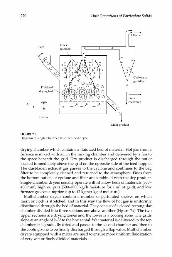
270 Unit Operations of Particulate Solids
drying chamber which contains a fluidized bed of material. Hot gas from a furnace is mixed with air in the mixing chamber and delivered by a fan to the space beneath the grid. Dry product is discharged through the outlet located immediately above the grid on the opposite side of the feed hopper. The dust-laden exhaust gas passes to the cyclone and continues to the bag filter to be completely cleaned and returned to the atmosphere. Fines from the bottom outlets of cyclone and filter are combined with the dry product. Single-chamber dryers usually operate with shallow beds of materials (300–400 mm), high outputs (500–1000 kg/h moisture for 1 m2 of grid), and low furnace gas consumption (up to 12 kg per kg of moisture).
Multichamber dryers contain a number of perforated shelves on which mesh or cloth is stretched, and in this way the flow of hot gas is uniformly distributed through the bed of material. They consist of a closed rectangular chamber divided into three sections one above another (Figure 7.9). The two upper sections are drying zones and the lower is a cooling zone. The grids slope at an angle of 2–3° to the horizontal. Wet material is delivered to the top chamber, it is gradually dried and passes to the second chamber and then to the cooling zone to be finally discharged through a flap valve. Multichamber dryers equipped with a mixer are used to ensure more uniform fluidization of very wet or finely divided materials.
Feed
Air
Heater
Fluidizeddrying bed
Finesreleased
Main product
Finesrecovered
Cyclone orgas filter
Clean air
Figure 7.8Diagram of single-chamber fluidized-bed dryer.

Fluidization 271
Design equations used to determine drying time and dimensions of the drying equipment are required in order to develop methods of drying diverse materials in a fluidized bed. These equations should be derived on the basis of theoretical analysis of a physical model of the process, as well as on experimental determinations of the influence of the most important factors on its kinetics. Drying is a complex heat and mass transfer process including a number of additional effects which may cause undesirable characteristics in the product, such as shrinkage or case hardening. Drying in a fluidized bed has special features: the particles of moist material receive heat from a flow of gas, which acts both as a heat transfer and a fluidizing medium. The gas bulk flow rate is limited because the gas velocity in the drying chamber must be limited to avoid excessive entrainment of material. Difficulties could also arise because motion of individual particles of mate-rial in the drying zone is indeterminate and they may rotate, change in size,
Hot gas
Hotgas
Cold air
Feed
Exhaust air
Chamber
Product
Coolingair
Figure 7.9Multichamber fluidized-bed dryer.

272 Unit Operations of Particulate Solids
and agglomerate. Furthermore, a proportion of the gas phase passes through the bed in the form of bubbles.
In fluidized-bed drying, normally the limiting kinetic factor is the process of external transfer of surface moisture from the material to the surrounding medium. In such a case, temperature gradients and variations in moisture content within the material are usually small and, thus, the material tempera-ture is assumed constant and equal to the wet bulb temperature. The mecha-nism of heat transfer of the process is, therefore, considered to be convective. Under these circumstances it is assumed that the quantity of heat supplied determines the quantity of moisture evaporated. In drying processes by convective mechanism, at least two drying periods are recognized: a constant rate period and a falling rate period. The duration of the constant rate period is generally calculated from an energy balance using heat transfer equations. The most difficult problem is to determine the duration of the falling rate period. In practice, experimental drying curves are often used to determine the critical moisture content of the material. The tests are carried out on a small model which must reproduce the drying conditions such as tempera-ture, air humidity, air velocity, and so on. During this falling rate period, the temperatures of the material and drying agent rise at all points in the fluidized bed. The distribution of the quantity of heat between evaporating moisture and heating the wet material is a function of the kinetics of internal heat and mass transfer. Equations that include the constant and falling rate periods have been proposed. For example, for drying grains in a spouted bed, an expression describing isothermal diffusion within grains is
w ww w n
n x
n
−− = −
=
∞
∑s
s2
12
1
2 2 26 19ππ
exp
(7.26)
where
x
SV
Dt= p
p (7.26b)
In Equations 7.26 and 7.26b w is the moisture content of the material at time t, ws is the surface moisture content of the material, w1 is the initial moisture content of the material, Sp is the surface area of particles, Vp is the particle volume, and D is the diffusion coefficient.
7.3.4 Coating of Particles and Particulates
Coating or encapsulation of particles, granules, or particulates can be carried out by a number of unit operations. Some of the operations used for mixing or dry powders can be equally applied for coating. Equipment that can be used for the purpose of mixing powders/coating particulates includes

Fluidization 273
rotating drums, ribbon mixers, and fluidized beds (Ortega-Rivas, 2005). Fluidized-bed coating was developed in the 1950s, and it is normally known as “Wurster process” (Arshady, 1993). The application of the fluidized-bed technique for the coating of particles aims to manufacture a product of uni-form quality and morphology, which is basically determined by the actual physical state of the droplets (Eichler, 1989). Droplet formation, contact, spreading, coalescence, and evaporation, are occurring almost simultane-ously during the process (Jones, 1985). The nozzles typically used in fluid-ized-bed coating are either binary or pneumatic; liquid is supplied at a low pressure and is sheared into droplets by air. Droplet size and distribution are more controllable with this type of nozzle than with a hydraulic one, espe-cially at low liquid flow rates (Filková and Mujumdar, 1995). Furthermore, the air used for atomization also contributes to evaporation of the coating solvent, increasing the droplet viscosity and inhibiting spreading and coales-cence on contact with the core material (Jones, 1985). There have been several designs of fluidized-bed configurations over the years. The conventional top-spray method (Figure 7.10) evolved from fluidized-bed dryers. The par-ticles are accelerated from the product container past the nozzle, and so they are sprayed counter-currently by the stream of atomized droplets. The coated particles travel through the coating zone into the expansion chamber, falling back into the product container and continue cycling throughout the process (Jones, 1988). In the bottom-spray method (Figure 7.11) the particles are recy-cled through the coating zone in seconds, as in the top-spray technique, but the fluidization pattern is much more controlled. The droplets and particles travel cocurrently, avoiding almost completely premature droplet evapora-tion. The film-forming droplets can spread out at lowest viscosity, producing a very dense film (Mehta and Jones, 1985). A relatively new approach to coat-ing is the tangential-spray method, with a rotary base, as shown in Figure 7.12. A combination of three forces occurs during fluidization, which has been described as spiralling helix. A centrifugal force by a rotating disc causes the product to move toward the wall of the chamber, the air velocity through an annular gap provides acceleration upward, while gravity cas-cades the product inwards and toward the disc once again. Beneath the sur-face of a rapidly tumbling bed, a nozzle is positioned to spray the coating tangentially to and concurrently with the flow of particles (Jones, 1988).
A way of evaluating coating efficiency is by determining the deposited coating mass mc, and relating it to the coating solution dry matter content DM. Dewettinck and Huyghbaert (1998) have suggested the following expres-sion for the evaluation of coating efficiency Ec:
E
mmc
c
cs DM= ⋅
(7.27)
where mcs is the mass of the coating solution.

274 Unit Operations of Particulate Solids
Coating solution
Nozzle
Fluidized particles
Inlet air
Figure 7.10Diagram of top-spray fluidized-bed equipment.
Inlet airCoating solution
Nozzle
Air distribution plate
Fluidized particles
Figure 7.11Diagram of the bottom-spray (Wurster) fluidized-bed coater.

Fluidization 275
Coating thickness dc is sometimes difficult to measure conveniently due to the fine size of some powders and to the unevenness of the surface of some granular materials. A reasonably estimate of the coating thickness for spher-ical microcapsules can be calculated using the following expression (Dewettinck, 1977):
dm m
mx
cs
c
s c
s=
⋅ + −
+
−
⋅
ρρ 1 1 1
2
1 3/
(7.28)
where ρs is the density of the core material, ρc is the density of the coating material, ms is the mass of the core material, mc is the mass of the coating material, and x is an equivalent diameter of the core material.
An important advantage of fluidized-bed coating is its ability to minimize attrition of the particles being processed. Attrition represents one of the major problems in food powder processing with many adverse effects such as segregation of fines from the bed structure, degradation of product qual-ity, changes in bulk flow behavior, and reduction of reconstitutability of the product (Ortega-Rivas, 2005). The segregated fines can be released to the sur-rounding atmosphere causing dust emissions and constituting a safety prob-lem. Among all the problems associated with dust emissions, such as health hazards, abrasion damage to equipment, impaired visibility, and so on, the risk of dust explosion is one of the greatest concerns in many dry powder operations, such as industrial grain and cereal processing (Barbosa-Canovas et al., 2005).
Inlet air
Coating solution
Nozzle
Fluidized particles
Rotating disc
Figure 7.12Diagram of tangential-spray, rotor, fluidized-bed coater.

276 Unit Operations of Particulate Solids
Reduction of attrition can be also used as an indicative of the coating effi-ciency. A manner to determine degree of attrition in coated materials can be done by performing a friability test, which is widely used in different agglomerated and compacted food and pharmaceutical products. A friabil-ity tester consists, simply, of a rotating disc or drum on which materials are subjected to tumbling at different times and rotation speeds. Friability is determined as the difference of weighed sample before and after the test. The tumbling action in a friability tester replicates typical handling situa-tions, to predict how well coated products will withstand handling during transportation and storage.
7.4 Laboratory Exercise: Fluidized-Bed Coating of Food Particulates
7.4.1 introduction
Coating with sweet coverings is used in product development in the food industry, particularly in obtaining ready-to-eat breakfast cereals. Different edible coatings in cereals are applied in order to obtain advantages such as to enhance flavor, protect the food particulate from oxygen and moisture, or improve quality and functionality. A well applied and thick enough coat will be determinant in accomplishing these attributes and, also, will provide resistance to attrition or erosion due to handling and distribution. The exer-cise is aimed at testing different variables in coating food granules and veri-fying uniformity, thickness, and firmness of the applied coat.
7.4.2 equipment and Materials
A batch fluidized bed of the type of a Glatt® laboratory unit. Unsweetened puffed cereal, such as puffed wheat or puffed rice. Ingredients to prepare the coating syrup: sugar, cocoa, and water.
7.4.3 instruments and apparatuses
Optical microscope, analytical balance, friability tester.
7.4.4 operation of the Fluidized bed
Prepare 2–3 L of syrup mixing 80 g cocoa and 430 g sugar in 400 mL •water.Load the fluidizing unit with a batch of 400–500 g of the particulates.•

Fluidization 277
Operate the unit at ambient conditions and at an air velocity enough •to fluidize the particulates (1–3 m/s).Spray the syrup, once the particulates are completely suspended, at •a rate of about 15 mL/min.Run the process for 10, 15, and 20 min.•Stop the fluidizing unit and discharge the product.•Dry the coated granules placing them on a tray at room temperature, •or proceeding to a mild drying in a tray drier.
7.4.5 evaluation of the Coating Thickness
Cut out, very carefully, several thin slices of several granules coated •at different times.Observe them at the microscope.•Estimate the coat thickness by using an appropriate eyepiece •graticulate.
7.4.6 Friability Test
Weigh the sample and introduce it in the drum of the tester.•Run the tester, according to specific instructions of the apparatus. A •number of applications give satisfactory results at 20–25 rpm for 20–30 min.Unload the drum (if not done automatically) and weigh the pro-•cessed sample.
7.4.7 Calculations and report
Determine the coating efficiencies, using Equation 7.27, for the three •different samples. Record observations for further analysis.Compare the observed coat thicknesses with calculated thicknesses •using Equation 7.28, for the three treatments of samples.From friability testing determine friability as the difference of •weighed samples at the different conditions before and after the test. Express the friability in weight loss percentage.Present a complete written report, according to scientific report •guidelines, either given by instructor or consulted in the literature. Include graphs, charts, and calculations carried out. Include analysis from own data and, as much as possible, discussion based on litera-ture survey from studies and investigations on the subject.
278 Unit Operations of Particulate Solids
PROBLEMS
1. The approach velocity of a gas (ρ = 1.3 kg/m3, μ = 1.65 × 10⁻⁵ kg/m s) flowing through a bed of spherical particles is 0.032 m/s. If the bed is 2.9 m thick, determine the pressure drop developed.
2. A reactor contains catalyst particles shaped into cylinders 1.25 cm diameter and 2 cm high. A gas having a density of 1.28 kg/m3 and a viscosity of 1.73 × 10⁻⁵ Pa s flows at a steady rate through the bed, which has a voidage of 0.4. If the superficial velocity established is 0.6 m/s and the pressure drop through the bed is 2.5 kPa, calculate the bed height.
3. Anthracite coal of 1500 kg/m3 density is to be fluidized with air at 140 kPa in a vessel 3 m in diameter. 48 tons of coal, ground to an average diameter of 70-mesh (US Standards) are placed in the vessel, which is filled to a height of 2 m. Calculate the static void fraction and the minimum void fraction at height for fluidization.
4. Calculate the air velocity required to fluidize 50 kg of a polymer consisting on spherical particles of 3 mm diameter and 700 kg/m3 density. The fluidized medium is air of 1 kg/m3 density and 1.6 × 10⁻⁵ kg/m s viscosity. Estimate also the pressure drop if the particles are contained in a 40 cm diameter vessel.
References
Abrahamsen, A. R. and Geldart, D. 1980. Behaviour of gas fluidized beds of fine pow-der. Part I: Homogeneous expansion. Powder Technology 26: 35–46.
Arshady, R. 1993. Microcapsules for food. Journal of Microencapsulation 10: 413–435.Barbosa-Canovas, G. V., Ortega-Rivas, E., Juliano, P., and Yan, H. 2005. Food Powders:
Physical Properties, Processing, and Functionality. New York, NY: Kluwer Academic/Plenum Publishers.
Dewettinck, K. 1977. Fluidized Bed Coating in Food Technology: Process and Product Quality. PhD Thesis. Ghent, Belgium: University of Ghent.
Dewettinck, K. and Huyghbaert, A. 1998. Top-spray fluidized bed coating: effect of process variables on coating efficiency. Lebensmittel-Wissenchaft und Technologie 31: 568–575.
Eichler, K. 1989. Principles of Fluid-bed Processing. Binzen, Germany: Glatt GmbH.Epstein, N. and Mathur, K. B. 1982. Applications of spouted beds. In Handbook of
Multiphase Systems, Hetsroni, G. (ed.). New York, NY: McGraw-Hill.Ergun, S. 1952. Fluid flow through packed columns. Chemical Engineering Progress 48:
89–94.Filková, I. and Mujumdar, A. S. 1995. Industrial spray drying systems. In Handbook of
Industrial Drying, Vol. 1, Mujumdar, A. S. (ed.) New York, NY: Marcel Dekker.Jackson, R. 2000. The Dynamics of Fluidized Particles. Cambridge, UK: Cambridge
University Press.Jones, D. M. 1985. Factors to consider in fluid-bed processing. Pharmaceutical Technology
9: 50–62.
Fluidization 279
Jones, D. M. 1988. Controlling particle size and release properties. In Flavor Encapsulation, Risch, S. J. and Reineccius, G. A. (eds.) Washington, DC: American Chemical Society.
Mathur, K. B. and Gishler, P. E. 1955. A technique for contacting gases with coarse solid particles. AIChE Journal 1: 157–164.
McCabe, W. L., Smith, J. C., and Harriot, P. 2005. Unit Operations in Chemical Engineering. 7th Ed. New York, NY: McGraw-Hill.
Mehta, A. M. and Jones, D. M. 1985. Coated pellets under the microscope. Pharmaceutical Technology 9: 52–60.
Ortega-Rivas, E. 2005. Handling and processing of food powders and particulates. In Encapsulated and Powdered Foods, Onwulata, C. (ed.) Boca Raton FL, USA: CRC Taylor & Francis.
Rhodes, M. 1998. Introduction to Particle Technology. Chichester, UK: John Wiley & Sons.
Toomey, R. D. and Johnstone, H. F. 1952. Gaseous fluidization of solid particles. Chemical Engineering Progress 48: 220–237.
Wilhelm, R. H. and Kwauk, M. 1948. Fluidisation of solid particles. Chemical Engineering Progress 44: 201–218.
Zenz, F. A. and Othmer, D. F. 1960. Fluidization and Fluid-Particle Systems. New York, NY: Reinhold.

Part III
Separation Techniques for Particulate Solids


283
8Introductory Aspects
8.1 Different Mixtures Relevant in Industry
In the material processing industry a great number of raw materials and products formed by several components are treated. Not only mixtures involving phases of the same state of matter, but also two-phase and multi-phase systems are normally encountered in a number of processes. Many mixtures or multiphase systems often need to be purified or depurate in order to obtain products, as free as possible, from impurities. For example, caustic soda and salt are treated in evaporators, an important number of food products are dehydrated, some ceramic and colorants are filtered, while sugars and fruit juices may be centrifuged. Depuration or separation of mixture components can be carried out in a number of ways, and tech-nologies to do so involve the use of some kind of energy. The ways to sepa-rate based on heat or mass transfer constitute a series of well-studied unit operations, while the ones known as mechanical separations were some-what neglected in higher-education programs for a long time (Svarovsky, 2000). A common problem facing process engineers in day-to-day practice in different materials processing industries is selecting, optimizing, or operating techniques involving the separation of one or more components of a mixture or a complex fluid.
8.2 Classification of Separation Techniques
A number of unit operations have as fundamental purpose the separation of two or more components within a system. Mixtures and multiphase fluids previously mentioned are varied in the materials processing industries and include solutions, suspensions, dispersions, and solid blends. The compo-nents within these systems may include any of the three common states of matter (i.e., solid, liquid, or gas), and so different combinations are possible. There are many criteria used to determine the most suitable strategy to

284 Unit Operations of Particulate Solids
perform a specific separation. Some factors that could be considered to define or select a method of separation are
Differences in physical properties of the compounds•
Differences in chemical properties of the compounds•
Possibility of mass transfer•
Possibility of phase changes in some of the compounds•
Use of natural forces to achieve the separation•
Use of external forces to achieve the separation•
Analyzing briefly the above-listed criteria, it is evident that classification of separation techniques is not an easy task, and that it is complicated to even consider a unified categorization. There are a number of separation tech-niques bearing little or no interest for certain industries, while there are tech-niques forming a minimal part of a more general unit operation. For example, magnetic separation is a separation technique encompassed by a unit opera-tion of great importance in food engineering: the cleaning of raw materials. Independently of referring to a general interest classification or one of inter-est exclusively for a branch of engineering, two commonly used criteria to propose a classification of separation techniques are
Classification of the separation techniques according to those involv-•ing phase change or mass transfer from one phase to another, known as diffusional operations, and those that are useful in the separation of solid particles or drops of a liquid and that are generally based in the application of an external physical force, known as mechanical separations.
Classification based on the separation techniques according to the •different combinations possible due to the states of matter (phases) found in any bicomponent or multicomponent system.
Two possible classifications of separation techniques based on the above criteria are given in Tables 8.1 and 8.2.
8.3 Specific Techniques for Granular Materials
Several separation techniques listed in the previous section are used to sepa-rate finely divided solids within a bicomponent system (Rushton et al., 2000). A thorough understanding of particle technology principles will therefore be useful not only to design storage and conveying systems (Part I) or

Introductory Aspects 285
optimally operate processing equipments (Part II), but also in order to have a greater chance of success in selecting, designing, or operating a system that involves separation techniques were one of the phases is a powder or par-ticulate solid (Cheremisinoff, 1995). In this context, only some of the previ-ously listed techniques, for example, liquid–liquid and liquid–gas systems would be particularly related to particle technology. Diffusional operations related to heat and/or mass transfer are based on principles out of the scope of particle technology and are widely addressed in classical chemical engi-neering texts. This final part of the book will be, therefore, dedicated to the study of operations known as mechanical separations, mechanical–physical separation processes, or physical separations. The two kinds of two-phase systems that will be studied are the solid–solid and solid–fluid mixtures. The usual way to separate the components of a solid–solid system is in dry, making use of differences in properties such as size, shape, density, as well as electric or magnetic characteristics. For the case of the solid–fluid mixtures
Table 8.1
Classification of Separation Techniques Based on Diffusion Properties
Diffusional Operations Mechanical Separations
Phase equilibrium SievingDistillation SedimentationLeaching and extraction CentrifugationOperations of multicomponents by stages FiltrationDiffusion and mass transfer between stagesGas absorptionHumidification operationsSolids drying
Table 8.2
Classification of Separation Techniques Based on Involved Phases
Liquid–Liquid Systems
Liquid–Solid Systems
Liquids with Dissolved Solids
Solid–Gas Systems Solid Mixtures
Distillation Sedimentation Separation by membranes
Cyclones separation
Sieving
Liquid extraction Centrifugation Hydrometallurgical extraction
Gas filtration Electromagnetic separation
Decantation Hydrocyclone separation
Evaporation Gravitational methods
Electrostatic separation
Ionic exchange Filtration Crystallization of solutions
Scrubbing
Dieresis and electro dialysis
Drying of wet solids
Flotation
286 Unit Operations of Particulate Solids
the most common case is when a fluid is a liquid, usually water, and techniques of great industrial importance, such as filtration and centrifuga-tion are included.
References
Cheremisinoff, P. N. 1995. Solids/Liquids Separation. Boca Raton, FL: CRC Press.Rushton, A., Ward, A. S., and Holdich, R. G. 2000. Solid–Liquid Filtration and Separation
Technology. Weinhem, Germany: Wiley-VCH.Svarovsky, L. (ed.) 2000. Solid–Liquid Separation. Oxford: Butterworth-Heinemann.

287
9Solid Mixtures
9.1 Screening
9.1.1 basic Principles
Screening is a separation technique of a mixture of various sizes of solids particles into several fractions, based on size difference. It consists of forcing the mixture through a screen of a specific size aperture. Small-capacity plane screens are often called sieves. By vibrating or oscillating a screen, particles smaller than a given aperture pass through this being thus separated from the remaining mixture. Screens are made from metal bars, perforated or slotted metal plates, woven wire cloth, or fabric, such as silk bolting cloth. Metals used include steel, stainless steel, bronze, copper, nickel, and monel. The screen surface may be plane (horizontal or inclined) or it may be cylin-drical. The size aperture of the screens, range from about 0.1 mm to approxi-mately 250 mm, with exceptional cases in which the aperture may be as large as 460 mm.
Screening has two main applications: laboratory technique for particle size analysis, and industrial operation for fractionation and classification of particulate solids. Although screen aperture, defined as the space between the individual wires of a wire mesh screen, is the preferred terminology for screening operations, the former designation of mesh number, defined as the number of wires per lineal inch, is still widely adapted. In both applica-tions, shape and size of particles may influence separation and efficiency. A combined shape–size effect may cause blinding or clogging of the screen openings, and is particularly likely to occur when particles have sizes very close in dimension to the screen aperture. In general terms, there would be three defined possibilities of a given particle facing a screen aperture: (a) the particle being too large in relation to the aperture so that it would be easily retained, (b) the particle being too small in relation to the aperture so that it would go through easily, (c) the particle having a critical dimension so that it would be trapped and promote blinding or clogging of the screen surface. This mentioned critical dimension has been defined when the particle has an approximate size of 1.1D (Figure 9.1), which happens if the angle θ between the particle and the screen aperture is less than tan−1 μ, μ being the
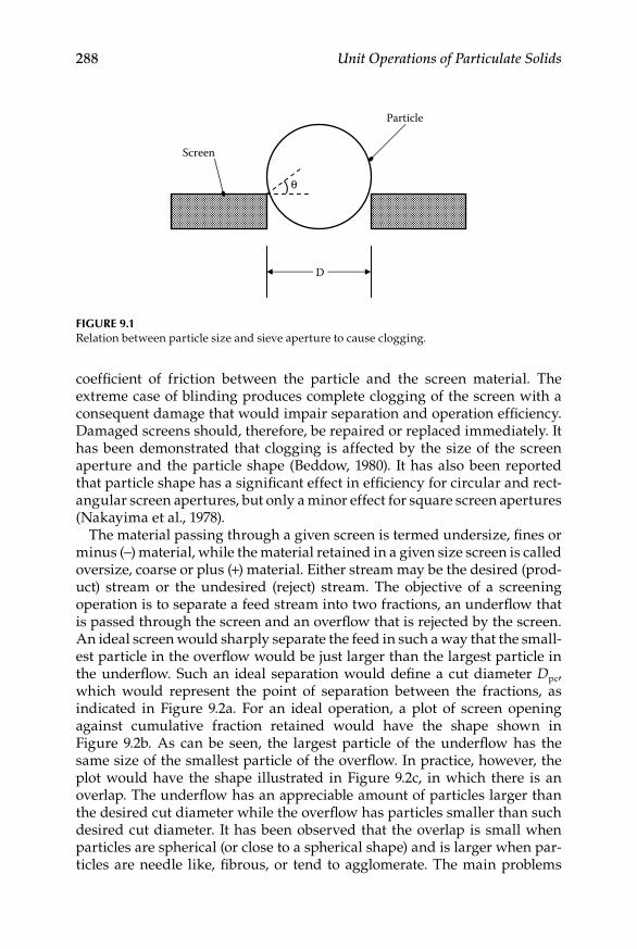
288 Unit Operations of Particulate Solids
coefficient of friction between the particle and the screen material. The extreme case of blinding produces complete clogging of the screen with a consequent damage that would impair separation and operation efficiency. Damaged screens should, therefore, be repaired or replaced immediately. It has been demonstrated that clogging is affected by the size of the screen aperture and the particle shape (Beddow, 1980). It has also been reported that particle shape has a significant effect in efficiency for circular and rect-angular screen apertures, but only a minor effect for square screen apertures (Nakayima et al., 1978).
The material passing through a given screen is termed undersize, fines or minus (−) material, while the material retained in a given size screen is called oversize, coarse or plus (+) material. Either stream may be the desired (prod-uct) stream or the undesired (reject) stream. The objective of a screening operation is to separate a feed stream into two fractions, an underflow that is passed through the screen and an overflow that is rejected by the screen. An ideal screen would sharply separate the feed in such a way that the small-est particle in the overflow would be just larger than the largest particle in the underflow. Such an ideal separation would define a cut diameter Dpc, which would represent the point of separation between the fractions, as indicated in Figure 9.2a. For an ideal operation, a plot of screen opening against cumulative fraction retained would have the shape shown in Figure 9.2b. As can be seen, the largest particle of the underflow has the same size of the smallest particle of the overflow. In practice, however, the plot would have the shape illustrated in Figure 9.2c, in which there is an overlap. The underflow has an appreciable amount of particles larger than the desired cut diameter while the overflow has particles smaller than such desired cut diameter. It has been observed that the overlap is small when particles are spherical (or close to a spherical shape) and is larger when par-ticles are needle like, fibrous, or tend to agglomerate. The main problems
θ
D
Particle
Screen
Figure 9.1Relation between particle size and sieve aperture to cause clogging.

Solid Mixtures 289
encountered in screening result from sample stickiness, sieve blockage, and agglomeration. According to Strumpf (1986), all these problems increase exponentially as the screen aperture decreases.
9.1.2 Design and Selection Criteria
The efficiency of a screening operation may be evaluated by simple mass balances. Let F be the mass flow rate of feed, O the mass flow rate of coarse fraction, and U the mass flow rate of fines; also, let XF be the coarse mass fraction in the feed, XO the coarse mass fraction in the overflow and XU the coarse mass fraction in the underflow. Furthermore, the fines fractions in the feed, the overflow and the underflow would be 1 − XF, 1 − XO, and 1 − XU,
DpcDpc
O
U
O
U
Aperture size
Cum
ulat
ive o
vers
ize f
ract
ion
0
1.0
1.0(a)
(b) (c)
0
Dpc
U
O
Aperture size
Cum
ulat
ive o
vers
ize f
ract
ion
Figure 9.2Diagram of cumulative frequency of oversized particles for: (a) feed, (b) ideal separation, and (c) real separation.
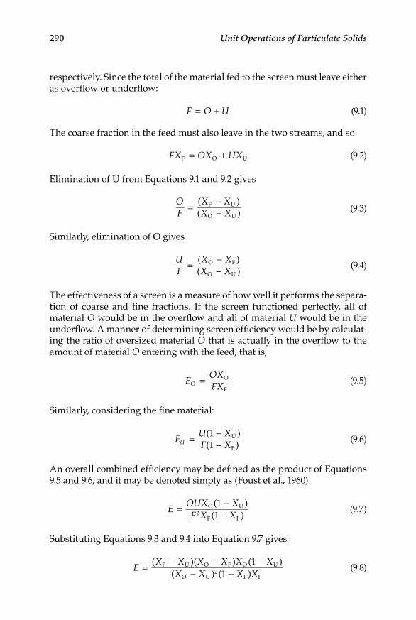
290 Unit Operations of Particulate Solids
respectively. Since the total of the material fed to the screen must leave either as overflow or underflow:
F O U= + (9.1)
The coarse fraction in the feed must also leave in the two streams, and so
FX OX UXF O U= + (9.2)
Elimination of U from Equations 9.1 and 9.2 gives
OF
X XX X
= −−
( )( )
F U
O U (9.3)
Similarly, elimination of O gives
UF
X XX X
= −−
( )( )
O F
O U (9.4)
The effectiveness of a screen is a measure of how well it performs the separa-tion of coarse and fine fractions. If the screen functioned perfectly, all of material O would be in the overflow and all of material U would be in the underflow. A manner of determining screen efficiency would be by calculat-ing the ratio of oversized material O that is actually in the overflow to the amount of material O entering with the feed, that is,
E
OXFXO
O
F=
(9.5)
Similarly, considering the fine material:
E
U XF XU = −
−( )( )11
U
F (9.6)
An overall combined efficiency may be defined as the product of Equations 9.5 and 9.6, and it may be denoted simply as (Foust et al., 1960)
E
OUX XF X X
= −−
O U
F F
( )( )
112
(9.7)
Substituting Equations 9.3 and 9.4 into Equation 9.7 gives
E
X X X X X XX X X X
= − − −− −
( )( ) ( )( ) ( )
F U O F O U
O U F F
112
(9.8)
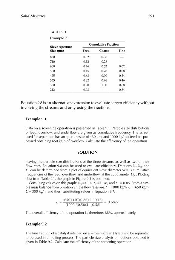
Solid Mixtures 291
Equation 9.8 is an alternative expression to evaluate screen efficiency without involving the streams and only using the fractions.
example 9.1
Data on a screening operation is presented in Table 9.1. Particle size distributions of feed, overflow, and underflow are given as cumulative frequency. The screen used for separation has an aperture size of 460 μm, and 1000 kg/h of feed are pro-cessed obtaining 650 kg/h of overflow. Calculate the efficiency of the operation.
SoluTion
Having the particle size distributions of the three streams, as well as two of their flow rates, Equation 9.8 can be used to evaluate efficiency. Fractions XF, XO, and XU can be determined from a plot of equivalent sieve diameter versus cumulative frequencies of the feed, overflow, and underflow, at the cut diameter Dpc. Plotting data from Table 9.1, the graph in Figure 9.3 is obtained.
Consulting values on this graph: XO = 0.14, XF = 0.58, and XU = 0.85. From a sim-ple mass balance from Equation 9.1 the flow rates are: F = 1000 kg/h, O = 650 kg/h, U = 350 kg/h, and thus, substituting values in Equation 9.7:
E = −−
=( )( )( . )( . )( ) ( . )( . )
.650 350 0 86 1 0 15
1000 0 58 1 0 580 68272
The overall efficiency of the operation is, therefore, 68%, approximately.
example 9.2
The fine fraction of a catalyst retained on a 7-mesh screen (Tyler) is to be separated to be used in a melting process. The particle size analysis of fractions obtained is given in Table 9.2. Calculate the efficiency of the screening operation.
Table 9.1
Example 9.1
Sieve Aperture Size (μm)
Cumulative Fraction
Feed Coarse Fine
850 0.02 0.06 —710 0.12 0.28 —600 0.26 0.52 0.02500 0.45 0.78 0.08425 0.68 0.90 0.24355 0.82 0.96 0.46300 0.90 1.00 0.68212 0.98 — 0.84
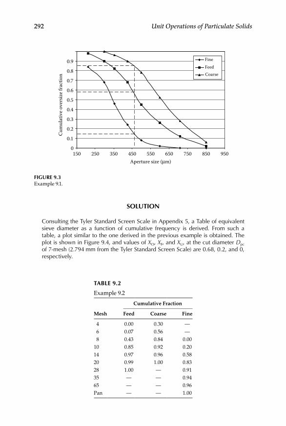
292 Unit Operations of Particulate Solids
SoluTion
Consulting the Tyler Standard Screen Scale in Appendix 5, a Table of equivalent sieve diameter as a function of cumulative frequency is derived. From such a table, a plot similar to the one derived in the previous example is obtained. The plot is shown in Figure 9.4, and values of XO, XF, and XU, at the cut diameter Dpc of 7-mesh (2.794 mm from the Tyler Standard Screen Scale) are 0.68, 0.2, and 0, respectively.
0
0.1
0.2
0.3
0.4
0.5
0.6
0.7
0.8
0.9
150 250 350 450 550 650 750 850 950Aperture size (μm)
Cum
ulat
ive o
vers
ize f
ract
ion
FineFeedCoarse
Figure 9.3Example 9.1.
Table 9.2
Example 9.2
Mesh
Cumulative Fraction
Feed Coarse Fine
4 0.00 0.30 — 6 0.07 0.56 — 8 0.43 0.84 0.0010 0.85 0.92 0.2014 0.97 0.96 0.5820 0.99 1.00 0.8328 1.00 — 0.9135 — — 0.9465 — — 0.96Pan — — 1.00
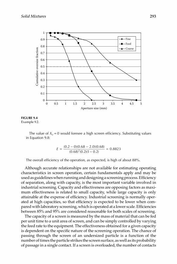
Solid Mixtures 293
The value of XU = 0 would foresee a high screen efficiency. Substituting values in Equation 9.8:
E = − −−
=( . )( . . )( . )( . ) ( . )( . )
.0 2 0 0 68 2 0 0 68
0 68 0 2 1 0 20 88232
The overall efficiency of the operation, as expected, is high of about 88%.
Although accurate relationships are not available for estimating operating characteristics in screen operation, certain fundamentals apply and may be used as guidelines when running and designing a screening process. Efficiency of separation, along with capacity, is the most important variable involved in industrial screening. Capacity and effectiveness are opposing factors as maxi-mum effectiveness is related to small capacity, while large capacity is only attainable at the expense of efficiency. Industrial screening is normally oper-ated at high capacities, so that efficiency is expected to be lower when com-pared with laboratory screening, which is operated at a lower scale. Efficiencies between 85% and 95% are considered reasonable for both scales of screening.
The capacity of a screen is measured by the mass of material that can be fed per unit time to a unit area of screen, and can be simply controlled by varying the feed rate to the equipment. The effectiveness obtained for a given capacity is dependent on the specific nature of the screening operation. The chance of passing through the screen of an undersized particle is a function of the number of times the particle strikes the screen surface, as well as its probability of passage in a single contact. If a screen is overloaded, the number of contacts
0
0.1
0.2
0.3
0.4
0.5
0.6
0.7
0.8
0.9
1
0 0.5 1 1.5 2 2.5 3 3.5 4 4.5 5Aperture size (mm)
Cum
ulat
ive o
vers
ize f
ract
ion
FineFeedCoarse
Figure 9.4Example 9.2.

294 Unit Operations of Particulate Solids
is small and the chance of passing on contact is reduced by particle interfer-ence. The improvement of effectiveness obtained at the expense of reduced capacity is a result of more contacts per particle and better chances for pass-ing through the screen aperture on each contact. A particle would have an ideal opportunity of passage when striking the surface perpendicularly, which would only be possible if it were oriented with its minimum dimen-sions parallel to the screen surface. Additional conditions would be no inter-ference by other particles, as well as not sticking to, or wedging into, the screen surface. None of these conditions apply to actual screening, but this ideal situation can be used as a basis for estimating the effect of mesh size and wire dimensions on screen performance. If the width of a screen would be negligible in comparison with the size of the openings, the wires would not interfere with particle passage and, practically, the entire screen surface would be active. In such a case, the probability of passage of a striking parti-cle would approach unity. In actual screening the diameter of the wire, or the fraction of the surface not constituting openings, is significant and the solid meshes strongly affect screen performance, especially by retarding the pas-sage of particles nearly as large as the screen openings. When large and small particles are present, the large ones tend to segregate in a layer next to the screen preventing the smaller particles from reaching the screen surface. All these factors tend to reduce capacity and lower efficiency.
Based on the information given and discussed above, a processing engi-neer should be able to evaluate capacity and efficiency for a particular screen-ing industrial operation. In order to avoid problems and come up with the most suiTable choice for a process involving screening, as important as these mentioned characteristics, other details can be equally important. Structural supports will be under varying conditions and so attention must be given to adequately sizing them, not only for the loads to be carried out but for the deflection and vibratory conditions that could prevail in operation. Feed and product chutes also deserve careful consideration. The feed to the screen must be delivered so as to cause minimal amount of abrasion or disturbance of the bed of material on the screen. The trajectory of material being dis-charged from feed conveyors or other units of equipment must be considered, and the force of the falling material directed against an abrasive-resistant wear plate, or a dead-bed of the material itself. The screening operation should be considered within the context of a whole process flow sheet. A description of the unit operations immediately preceding and following is quite relevant. Details of the equipment adjacent to the screening step must be carefully con-sidered. For example, there is little point in dry screening a dusty material if the succeeding stages are wet. The screening operation involved should also describe the methods used for controlling feed rate, product collection, required screen efficiency, number and size of products, and so on.
Several relevant properties of the material being separated are to be known or determined to properly select or design appropriate screening equipment. Some of these include: particle size distribution, particle shape, bulk density,

Solid Mixtures 295
moisture content, abrasiveness, and corrosiveness. The particle size distribu-tion is essential to correctly size the screening unit, as well as to specify the type of screen to be installed. As previously mentioned, particle shape is determinant in promoting, or avoiding, blinding or clogging of screen units. Long or splinter-like, round or oval, or cubic particles will have slightly differ-ent screening characteristics, and may have a great influence on choice of cloth opening. Bulk density permits the determination of the volume of flow, and a measure of the load to be carried by the screen. Moisture content may cause difficulties due to stickiness. Information on moisture content, along with data on the process following screening, will allow selection of dry, damp, or wet screening. In some dry-screening applications, when moisture content is low, the choice of a proper screen medium will eliminate problems. Predrying of materials using heated screen cloths, or going wet by adding water sprays, are all equally effective in damp screening. The abrasive characteristics of the material have great influence on choice of materials of construction, as well as in selection of methods of loading, collecting, and transporting products. Corrosive features will also influence materials of construction used in screen frames, media, chutes, feedboxes, and other elements of the system. This prop-erty is relevant for choosing between dry and wet screening.
example 9.3
A granular material has been analyzed giving the results presented in Table 9.3. The product from which the sample was taken is separated using a screen of 1 mm opening, and the fine fraction is to be used for a specific process. The screen is fed at a rate of 8660 kg/h, obtaining 1960 kg/h of coarse material and, practically, no particles smaller than 1 mm. Since the fraction of interest is the fine one, calculate the efficiency of the operation, expressed as separation of fines.
SoluTion
In this case, tabulated data include only the particle size distribution of feed. The retained fraction is given, rather than the cumulative fraction. Following a proce-dure similar to that in Example 2.4, a plot of cumulative frequency can be obtained. Since Dpc is 1 mm, the feed fraction XF can be read directly from Table 9.3, as
Table 9.3
Example 9.3
Particle Size Range Weight (g)
Larger than 2 mm 0.0Between 2 and 1 mm 19.8Between 1 and 0.5 mm 58.2Between 0.5 and 0.1 mm 10.2Smaller than 0.1 mm 11.8

296 Unit Operations of Particulate Solids
0.198. From a mass balance using Equation 9.1, U = 6700 kg/h. Since there are no fines within the coarse stream, fractions XO and XU are 1.0 and 0, respectively. Substituting into Equation 9.6:
EU = −−
=( )( )( )( . )
.6700 1 0
8660 1 0 1980 9646
The efficiency, expressed in terms of separation of fines is, thus, 96.5% approximately.
9.1.3 equipment used
Screening as a unit operation may be carried out in different types of equip-ment. Three types are more common: grizzlies (bar screens); shaking, vibra-tory or oscillating screens; and revolving screens or trommels. Grizzlies are used for screening larger particles (pieces greater than 25 mm). They consist of a set of parallel bars, spaced to the desired separation. The bars are often wedge shaped to minimize clogging. They may be used horizontally or inclined at angles up to 60°. Vibrating grizzlies are available, the feed mate-rial passing over the screening surface in a series of jerks.
The machines simply termed as screens can consist of many types: vibrat-ing, shaking, reciprocating, and oscillating, to name only a few. Industrial screening equipment is used over a wide range of particle sizes. For small particles woven cloth or wire screen are used, while for larger sizes perfo-rated metal plates or grids can be employed. Dynamic screening equipment can be classified according to the type of motion used to shake up and trans-port the material on the screen. Vibrating screens are used as standard prac-tice when large capacity and high efficiency are required. The capacity, particularly in the finer sizes, is greater by far when compared with any other of the screen types, so that they are normally preferred when efficiency of the screen is the governing factor of a given process. Other advantages of vibrating screens include accuracy of sizing, increased capacity per unit area, low maintenance costs, and saving in installation space. The screens used in this type of equipment can be mounted horizontally or inclined and their operating range of frequencies is high (1000–7000 Hz).
Shaking screens consist on a rectangular frame, holding wire cloth or per-forated plate, slightly inclined and suspended by loose rods or supported from a base frame by flexible flat springs. The frame is driven with a recipro-cating motion, and the material to be screened is fed at the upper end advanc-ing by the forward stroke of the screen. As the feed advances on the screen surface, finer particles pass through the screen openings. Shaking screens may be conventionally used for both screening and conveying of a num-ber of materials. Their advantages include the low headroom and power requirement, while some disadvantages are the high maintenance cost of the screen and the supporting structure due to vibration, and the low capacity compared to inclined high-speed vibrating screens.

Solid Mixtures 297
Reciprocating screens are operated with a shaking motion, long stroke, at frequencies between 20 and 200 Hz. They produce size fractions removing the coarse material first and the fines last. These machines contain several decks of screens, one above the other, held in a box or casing. The coarsest screen is located at the top while the finest is mounted at the bottom. Suitable discharge ducts allow proper removal of the several fractions. Figure 9.5 shows a diagram of a reciprocating screen. The feed is dropped on the top screen, and screens and casing are gyrated in order to sift the parti-cles through the screen openings. In the vertically gyrated design the casing is inclined at an angle of 16–30° to the horizontal plane. The gyrations are vertically about the horizontal axis. The screens are rectangular shaped and fairly long, with typical dimensions of 0.46 × 1.2 m to 1.5–4.3 m. The speed of gyration and the amplitude of throw are adjustable, and also is the angle of tilt. A particular combination of speed and throw would normally give the maximum yield of required product from a given speed. Satisfactory separa-tion into fine fractions usually requires an angle not more than 20°. A hori-zontally gyrated screen design contains rectangular slightly inclined screens, which are gyrated at the feed end. The discharge end reciprocates but does not gyrate. This combination of motions stratifies the feed, so that fine par-ticles travel downward on the screen surface, where they are pushed through the opening on the screen by the larger particles moving on top. The screen surface is often double, as shown in Figure 9.5. Between the two screen sur-faces rubber balls are positioned and held in separate compartments. As the screen operates, the rubber balls strike the screen surfaces, freeing the opening of any material that would tend to plug them.
Feed
Upper screen
Ball cleaners
Finefraction
Coarsefraction
Eccentric
Lower screen
Figure 9.5Horizontally gyrated reciprocating screen.

298 Unit Operations of Particulate Solids
Oscillating screens usually operate at gentle speeds, between 300 and 400 oscillations/min, and with a long linear stroke. The motion of the screen is of an orbital nature, practically on the plane to the screen deck, and may be transmitted by high-velocity eccentrics to the sieves. Vibration is accom-plished by eccentric weights on the upper and lower ends of the motion-generator shaft. Rotation of the top weight creates vibration in the horizontal plane, which causes the material to move across the screen cloth to the periphery. The lower weight acts to tilt the machine, causing vibration in the vertical and tangential planes. The angle of lead given the lower weight with relation to the upper weight provides variable control of the spiral screening pattern. Speed and spiral pattern of material travel over the screen cloth can be set by the operator for maximum throughput. Oscillating screen units are box-like machines, either round or square, with a series of screen nested atop one another. The sieves are made of wire mesh or perforated screen decks to separate relatively dense, dry, undersized materials, from less dense over-sized materials. A schematic diagram of an oscillating round screen is given in Figure 9.6.
Reels or trommels are revolving cylindrical screens mounted almost hori-zontally, with one extreme opened. Their screening surface may consist of wire mesh or perforated sheet. Hexagonal cross sections are also used since these lead to agitation which aids the separation of fine material. Figure 9.7 shows a simple design or revolving screen. The feed material, which travels through the openings increasing in size along the drum, is discharged by a chute on the lower extreme of the equipment. Several arrangements of
Coarsefraction
Feed
Screen
Finefraction
Figure 9.6Diagram of oscillating round screen.

Solid Mixtures 299
trommels can be made to accomplish separation according to specific process requirements. Figure 9.8 presents two of them. The simplest case is when the drum perforations are uniform all over the surface. In such a case, to sepa-rate different fractions of a given material, the drums are mounted in series. Two alternatives may arise, in that the drum with the larger perforations is located as the first or the last of the series. When the largest perforations drum is the first of the series, the most convenient arrangement is to place the drums on top of the other (Figure 9.8a), so as to send the finest fraction of material to the following screen and successively. On the other hand, if the largest perforations drum is the last of the series the coarsest fraction advance to the next drum, and a more convenient arrangement will be to have them mounted one right after the other as a series-consecutive drum screen. Some other arrangements include the concentric drum arrangement illustrated in Figure 9.8b. This particular mounting has the advantage of compactness but, since the feed enters at the center, the smallest screen area will handle the complete feed load while the smaller fines fractions will be progressively processed into the larger screen areas.
The capacity of a trommel increases with increasing speed of rotation until a critical speed is achieved. At speeds greater than this, the material does not cascade over the surface but is carried round and centrifugal force and sepa-ration is seriously impaired. The critical speed of a trommel is given by
N
D= 42 3
1 2
.( ) /
(9.9)
where N is the number of revolutions of the trommel per minute, and D is the diameter of the trommel in meters.
Feed
Screens
Discharge
Figure 9.7Single drum revolving screen.

300 Unit Operations of Particulate Solids
Feed(a)
(b)
Coarsest fraction
Finest fraction
Feed into centralscreen
Smallestperforations
Largestperforations
Finestfraction
Coarsestfraction
Figure 9.8Arrangements for revolving screens: (a) parallel type and (b) concentric drum.

Solid Mixtures 301
9.2 Electromagnetic Separation
9.2.1 basic Principles
A particle of a given material exposed to a magnetic field will become magnetized to some extent and may act as a magnetic dipole. When plotting the intensity of the applied magnetic field H and the magnetization induced in the particle M, the resulting graphs represent the three ways in which magnetized materials may behave (Kolm, 1975). The materials thus classified, as illustrated in Figure 9.9, are: ferromagnetic, paramagnetic (magnetically attracted), and diamagnetic. The relationship M/H is known as the suscepti-bility. Paramagnetic substances have positive susceptibilities, and induced magnetization increases the magnetic-flux density within the substance. Diamagnetic materials have negative susceptibilities, and an induced field in this case cancels part of the magnetic-field intensity. Permeability μ, which is often used somewhat imprecisely in referring to ferromagnetic substances, is the ratio of the magnetic-flux density to the magnetic-field density. Magneti-zation of different materials is dependent directly on the degree of magnetic susceptibility and the applied magnetic field intensity. As can be seen in Figure 9.9, ferromagnetic materials quickly become magnetically saturated so
Indu
ced
mag
netiz
atio
n (M
)
Magnetic field intensity (H )
Ferromagnetic
Dilute ferromagnetic
Paramagnetic
Diamagnetic
Figure 9.9Magnetic behavior of materials.

302 Unit Operations of Particulate Solids
that an increase in the intensity of the magnetic field bears no further effect after a certain point. Paramagnetic materials, on the other hand, follow a direct proportion for the magnetic-flux density and the magnetic-field inten-sity. Some of these substances cannot be, virtually, saturated.
Three types of magnetic fields can be identified: isodynamic, katadynamic, and anadynamic. As can be observed in Figure 9.10, in an isodynamic magnetic region the gradient of magnetic energy does not vary with an increase in the magnetic-field intensity. This type of magnetization is useful to concentrate particles according to slight differences in susceptibility. A katadynamic region is characterized by an increase in the gradient of mag-netic energy directly proportional to the magnetic-field intensity. In this region the higher gradients of magnetic energy, along with the higher inten-sity of the magnetic field, may be applied to a particle. The region of anady-namic field, in which the energy gradient is inversely proportional to the magnetic-field intensity, is particularly useful to separate particles of low paramagnetic susceptibility (Sun, 1976).
Magnetic separation processes work by establishing a specific equilibrium among magnetic forces, particle–particle forces, and inertial forces acting on the particle. All these forces compete in a given operation, and so the role of a design exercise consists on allowing interaction to act in such a way that separation of particles may become feasible. Feed on a magnetic separator can be divided into two or more streams. The “tailings” are the magnetic product, the “mags” are the magnetic concentrate, and the “middlings” are a product lower in magnetization that can also be obtained.
Magnetic filed intensity
Mag
netic
ener
gy g
radi
ent Anadynamic
Katadynamic
Isodynamic
Figure 9.10Types of magnetic fields.

Solid Mixtures 303
9.2.2 equipment and applications
Magnetic separators may be classified into conventional separators and high-gradient separators. Table 9.4 lists the main types of equipment available to perform electromagnetic separations. Conventional processes are based on concentrating the magnetic material while the desired product may be either part: the magnetic or the nonmagnetic. Typical applications of conventional separators include removal of small iron pieces (wire, rivets, diverse iron fractions) from varied materials and mineral beneficiation of highly mag-netic minerals. Some applications of conventional magnetic separators are given in Table 9.5. There are three main designs of conventional magnetic separators: the grate separator, the drum separator, and the belt separator. The drum separator, whose schematic diagram is shown in Figure 9.11, is probably the equipment most widely used.
High-gradient magnetic separation may be considered an alternative to flotation and extraction for treatment of fine solids suspended in water (Gaudin, 1974), which would categorize it as a solid–liquid separation tech-nique. There are, however, some applications for dry separations. A widely used high-gradient magnetic separator is the “Ferrofilter Franz.” A sche-matic diagram of this type of equipment is given in Figure 9.12. The equip-ment comprises a solenoid magnet, a magnetic return circuit, a stainless-steel filtration ribbon, and a large voidage magnetic matrix. The unit is operated discontinuously and the feed flow is parallel to the magnetic field. Although
Table 9.4
Electromagnetic Common Separators and Their Main Characteristics
Type Involved Forces
Approximate Value of Effective Magnetic Parameters
Strength Range (cm)
Field Gradient
(Gauss/cm)
Forcea (dyn/cm2)
Fe3O4 CuO
Grate Gravity 1 500 3 × 10⁵ 5Drum Gravity,
hydrodynamic drag5 500 3 × 10⁵ 5
Belt Gravity 1–10 100–1000 5–50 × 104 0.2–20Davis tube Gravity,
hydrodynamic drag1 4000 2 × 10⁶ 3 × 10²
Frantz: isodynamci
Gravity 1 2000 1 × 10⁶ 4 × 10²
Frantz: ferrofilter
Hydrodynamic drag 0.1 1 × 10⁵ 1 × 10⁸ 2 × 10⁴
Jones Hydrodynamic drag 0.1 2 × 10⁵ 1 × 10⁸ 8 × 10⁴
Kolm-Marston
Hydrodynamic drag 0.001 2 × 10⁶ 1 × 10⁹ 8 × 10⁵
a For a particle whose diameter is equal or smaller than the range of magnetic force.

304 Unit Operations of Particulate Solids
S N
N
Feed
Rotating drum
Magnets
“Mags”
Figure 9.11Conventional drum magnetic separator.
Table 9.5
Typical Applications of Magnetic Separators
Iron Pieces RemovalFood processing
Manufacture of Chemical products•Mineral beneficiation•Manufacture of pharmaceuticals•Cooling fluids treatment•
Mineral Beneficiation
Iron recoveryFrom solid waste•From heavy media•

Solid Mixtures 305
this equipment is exclusively used in the kaolin industry for slurry separa-tions, several designs based on it have been developed for dry separation applications. The high-gradient magnetic dry separators can be fed by gravity or within an airstream, and they can handle materials as fine as 325-mesh in size. An example of application of this type of equipment is the separation of paramagnetic impurities from finely pulverized dry minerals (Iannicelli, 1976).
Some other types of high-gradient magnetic separators include the car-rousel continuous separator and the superconductive separator. The carrou-sel-type separator consists on a wheel containing cells where iron fiber matrices are fixed. As the wheel turns, the cells pass continuously near a highly magnetized field region where feed is introduced. The magnetic par-ticles are trapped inside the matrices, and when the cell goes far from the magnetized region the particles are removed by washing. The supercon-ductive separator is based on the low electric resistance showed by some materials cooled at certain temperature. These materials are known as superconductors, and their resistance may be reestablished by applying a specific electrical current or by placing the material in a magnetic field with intensity over a critical value. The magnetic field can, thus, act as a solenoid
Feed
Screens
Nonmagneticmaterial
Figure 9.12High-gradient magnetic separator.

306 Unit Operations of Particulate Solids
for the superconductive material, without elevating the temperature more than a Joule (Watson, 1979).
9.2.3 Selection Criteria
High-gradient magnetic separations are very sensitive to process variables. When a paramagnetic particle is trapped by a ferromagnetic wire and exposed to a magnetic-field intensity H, it is interesting to know the relation among the particle radius b, the wire radius a, and the force exerted by the wire on the particle. Theoretical calculations suggest that the magnetic strength depends critically on the radii of particle and wire, as shown in Figure 9.13 (Kolm, 1975). The attractive force between the particle and the wire reaches a maximum when the relation a/b attains a value of 2.69. A system in which particle and wire radii are adjusted to a maximum mag-netic strength value is known as a fixed system, and is effective only on certain ranges of particle size.
Kolm (1975) has studied the effect of increasing particle radius for the case of cupric oxide exposed to magnetic fields, and some data are reported as a plot in Figure 9.14. The Figure shows the plot of the relation of the magnetic force to the added opposite (gravity and drag) forces against particle radius. Clearly, a particle within the size range of 100 μm is the most appropriate for
0.01b 0.1b 1b 10b 100b10–5
10–4
10–3
10–2
10–1
1
Particle radius = b
Cable radius (a)
Mag
netic
forc
e (F m
)
Figure 9.13Plot of magnetic force versus wire diameter of a ferromagnetic wire.

Solid Mixtures 307
the fitted system and separation of particles far from that size range will become difficult.
9.3 Electrostatic Separation
9.3.1 basic Principles
Electrostatics may be defined as the study of stationary electrical charges, under conditions in which positive and negative parts are separated from each other. Electrostatic separation is accomplished by use of forces acting on charged or polarized bodies in an electrical field. Several methods can be used for charging, and include conductive induction, contact electrification, and ion bombardment. Conductive induction and ion bombardment are used to separate conductive materials from nonconductive materials. Examples of conductive materials include ilmenite, rutilium, galena, pyrite, and specularite. Among nonconductive materials quartz, zirconium, mona-zite, and diamonds can be mentioned. Contact electrification is usually employed to separate nonconductive materials, such as phosphoric rock and quartz, based on their degree of conductivity.
Conductive induction principle is illustrated in Figure 9.15. A charged body moves toward an isolated metal object B. Since similar charges reject while different charges attract, negative charges on object A induce electrons
0.1 1 10 100 1 × 10³ 1 × 10⁴ 1 × 1050
2
4
6
8
10
Particle radius (μm)
F m(F
d + F
g)
Fm = Magnetic force Fg = Gravity force Fd = Friction force
Figure 9.14Plot of fixed system for high-gradient magnetic separation of CuO.
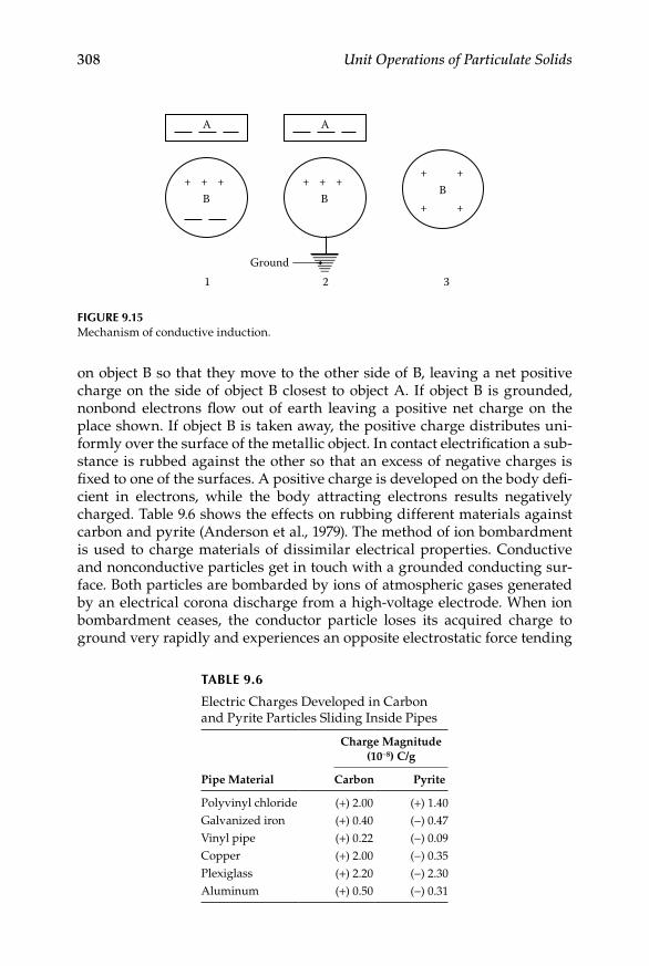
308 Unit Operations of Particulate Solids
on object B so that they move to the other side of B, leaving a net positive charge on the side of object B closest to object A. If object B is grounded, nonbond electrons flow out of earth leaving a positive net charge on the place shown. If object B is taken away, the positive charge distributes uni-formly over the surface of the metallic object. In contact electrification a sub-stance is rubbed against the other so that an excess of negative charges is fixed to one of the surfaces. A positive charge is developed on the body defi-cient in electrons, while the body attracting electrons results negatively charged. Table 9.6 shows the effects on rubbing different materials against carbon and pyrite (Anderson et al., 1979). The method of ion bombardment is used to charge materials of dissimilar electrical properties. Conductive and nonconductive particles get in touch with a grounded conducting sur-face. Both particles are bombarded by ions of atmospheric gases generated by an electrical corona discharge from a high-voltage electrode. When ion bombardment ceases, the conductor particle loses its acquired charge to ground very rapidly and experiences an opposite electrostatic force tending
Table 9.6
Electric Charges Developed in Carbon and Pyrite Particles Sliding Inside Pipes
Pipe Material
Charge Magnitude (10−8) C/g
Carbon Pyrite
Polyvinyl chloride (+) 2.00 (+) 1.40Galvanized iron (+) 0.40 (−) 0.47Vinyl pipe (+) 0.22 (−) 0.09Copper (+) 2.00 (−) 0.35Plexiglass (+) 2.20 (−) 2.30Aluminum (+) 0.50 (−) 0.31
B BB
+
+
+
+
A A
321Ground
+ ++ + ++
Figure 9.15Mechanism of conductive induction.

Solid Mixtures 309
to repel it from the conducting surface. The nonconducting particle side kept away from the conducting surface becomes coated with ions of charge oppo-site in electrical polarity to that of the surface, and it experiences an electro-static force tending to hold it to the surface. If the electrostatic force is larger than the force of gravity or other forces tending to separate the nonconduct-ing particle from the conducting surface, the particle is held in contact with the surface and is said to be “pinned.”
Particles can also be charged by comminution. It has been demonstrated that, in the millimeter range, charging by comminution does not produce particles with sufficient charge as to be influenced by an electrical field (Lawver, 1969). Within the micrometer range, however, it has been found that the resulting charge is high enough for the particles to show an electri-cal response, rather than a gravitational one, in an electric field. For homo-geneous substances, comminution will produce particles somewhat balanced in terms of electrical charges, so that electrostatic separation would not be a feasible option. Particles differing in chemical composition are satisfactorily charged by comminution, and electrostatic separation should give appropriate results.
9.3.2 equipment and applications
Table 9.7 gives a list of industrial applications of electrostatic separation (Lawver, 1969). The different types of equipment make use of either direct or alternating current sources in the range of 3 × 10³–3 × 10⁶ V/m. The high- tension sources used in commercial electrostatic separators cover a range as high as 250 × 103 V, but the power used is really lower, with a maximum value of 0.5 kW/h per ton of feed. Direct current is used to produce charge by conductive induction and ion bombardment, while alternating current is used to produce charge by polarization.
Table 9.7
Typical Industrial Applications of Electrostatic Separators
Minerals Combination Surface Treatment Usual Charge Mechanism
Hematite-quartz Drying Ion bombardmentLimenite-rutile Washing and drying Ion bombardmentZirconium-ilmenite Drying Ion bombardmentCassiterite-scheelite Drying Ion bombardment
Conductive inductionFeldspar-quartz Drying Contact electrificationHalite-silvanite Heating to 340°C Contact electrificationPyrite-carbon Drying Ion bombardment
Conductive inductionCarbon-chalkboard Moisture control Conductive inductionDiamond-silicon Washing and drying Conductive induction
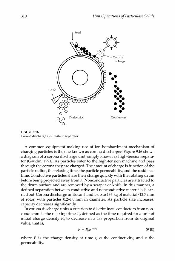
310 Unit Operations of Particulate Solids
A common equipment making use of ion bombardment mechanism of charging particles is the one known as corona discharger. Figure 9.16 shows a diagram of a corona discharge unit, simply known as high-tension separa-tor (Gaudin, 1971). As particles enter to the high-tension machine and pass through the corona they are charged. The amount of charge is function of the particle radius, the relaxing time, the particle permeability, and the residence time. Conductive particles share their charge quickly with the rotating drum before being projected away from it. Nonconductive particles are attracted to the drum surface and are removed by a scraper or knife. In this manner, a defined separation between conductive and nonconductive materials is car-ried out. Corona discharge units can handle up to 136 kg of material/12.7 mm of rotor, with particles 0.2–1.0 mm in diameter. As particle size increases, capacity decreases significantly.
In corona discharge units a criterion to discriminate conductors from non-conductors is the relaxing time Tr, defined as the time required for a unit of initial charge density P0 to decrease in a 1/e proportion from its original value, that is,
P P= −0e t/σ ε
(9.10)
where P is the charge density at time t, σ the conductivity, and ε the permeability.
ConductorsDielectrics
Coronadischarge
Feed
Knife
Figure 9.16Corona discharge electrostatic separator.

Solid Mixtures 311
Relaxing time for pyrite is approximately 10−3 s, while that for quartz is about 106 s. Quartz is, therefore, considered a nonconductor due to its long relaxing time, while pyrite is considered a conductor because of its short relaxing time.
Apart from the corona discharge unit, two common types of electrostatic separators are the plate separator and the screen–plate separator, illus-trated in Figure 9.17. Induction is used in both units to charge the feed
Feed
(a)
(b)
Plate (+)Electrode (–)
Conductors
Nonconductors
Plate (+)Electrode (–)
Feed
Screen
Nonconductors
Conductors
Figure 9.17Electrostatic separators: (a) plate type and (b) screen–plate type.
312 Unit Operations of Particulate Solids
particles. Efficiency of separation is lower for plate and screen–plate separators than that for corona discharge separators. For this reason, these types of units are mounted in series, with as much as five separation stages (Anonymous, 1976).
9.3.3 applications in Fine Particulate Systems
In order to attain satisfactory results when using electrostatic separations for finely pulverized materials, some alternatives have been suggested. It has been reported a fluidized bed design specially modified to avoid drag of particles within the gas stream (Kiewlet et al., 1978). It was found that a combination of low gas flow and mechanical vibration may fluidize effi-ciently a bed of fine particles minimizing the drag problem. Results for a synthetic mixture of glass and iron powders, sized between 15 and 55 μm, are given. Effects of temperature, moisture, and voltage were investigated for a mixture 50/50, by weight, of the mentioned materials. Three important conclusions were found: vibration along with fluidizing action may extend the use of electrostatic separation to mixtures of fine powders difficult to fluidize by gas stream only; vibration does not minimize the extracting effect, since recovering efficiencies well over 60% were observed for the steel component; temperature and voltage are the most determinant variables of the operation.
Another method to separate fine particles by electrostatic separation is the case of a dilute phase closed electrostatic circle (Inculet et al., 1977), devel-oped to eliminate the drag normally associated when handling particles below 40 μm in size. Due to the electric field influence, particles are deflected from the main stream trajectory and are extracted by central collectors. Particles are suspended in a gas stream, introduced to the loop by gas induc-tors consisting of two concentric rotating cylinders. The corona charging sec-tions include high-voltage corona wires, while the electrostatic separation section is located within a segment of the loop 1.2 m long, in which the high-voltage electrodes produce a horizontal electric field. The feed system con-sists on a fluidized bed mounted laterally to the continuous loop.
9.4 Laboratory Exercise: Efficiency of Separation on Single-Stage Screening
9.4.1 introduction
Screening is a separation of materials on the basis of size as a means of preparing a product for subsequent operation. Screening is performed

Solid Mixtures 313
using equipment with one or two sieving surfaces. A single sieve provides two products. The product from the top is called the oversized or plus product while the one which passes through the screen is the undersized or minus product. Material passing one sieve surface but remaining on the next one in a double deck screen is an intermediate product. During ideal screening, the plus product contains only particles greater than the size of openings of the screen surface while minus product consists of particles smaller than the opening. Efficiency of screening, measured as the quan-tity of misplaced material in any of the streams, can be affected by many factors. Clogging is a serious problem that may have a tremendous impact in efficiency. Apart from particle size and shape, that may directly cause clogging, some other characteristics of the feed material, such as its mois-ture content, may also cause clogging diminishing efficiency of the separa-tion process. The objective of the experiment is to evaluate the effect of moisture content of the material fed to a screening process, in clogging and efficiency of the separation.
9.4.2 equipment and Materials
US standard test sieves series, or laboratory size oscillating round screen unit. Two batches of 5–10 kg of coarse sand, and fine sand.
9.4.3 instruments or apparatuses
Granatary scale and moisture balance.
9.4.4 Screening Procedure
Mix thoroughly two equal parts of coarse and fine sand. If using •standard test sieves, combine 100 g of coarse sand with 100 g of fine sand. If using screen equipment, prepare a sample according to the size of the unit. Separate a sample to determine the moisture content using the moisture balance.Use, for any of the cases above, a 0.355 mm sieve (45-mesh), and •establish it as the cut diameter Dpc. Operate the testing setup for the recommended time accordingly.Collect the underflow and overflow samples, weigh them, and ana-•lyze them for their particle size distributions using the set of sieves required and following the procedure given in Section 2.7. ( Labora tory exercise: particle size analysis by different methods.)Collect data and elaborate table and plots, like those derived for •Examples 9.1 and 9.2.
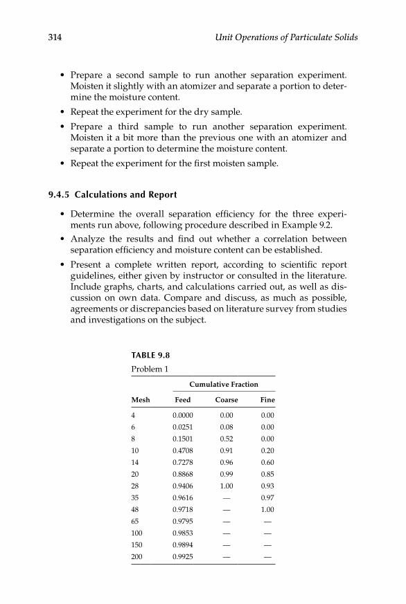
314 Unit Operations of Particulate Solids
Prepare a second sample to run another separation experiment. •Moisten it slightly with an atomizer and separate a portion to deter-mine the moisture content.
Repeat the experiment for the dry sample.•
Prepare a third sample to run another separation experiment. •Moisten it a bit more than the previous one with an atomizer and separate a portion to determine the moisture content.
Repeat the experiment for the first moisten sample.•
9.4.5 Calculations and report
Determine the overall separation efficiency for the three experi-•ments run above, following procedure described in Example 9.2.Analyze the results and find out whether a correlation between • separation efficiency and moisture content can be established.
Present a complete written report, according to scientific report •guidelines, either given by instructor or consulted in the literature. Include graphs, charts, and calculations carried out, as well as dis-cussion on own data. Compare and discuss, as much as possible, agreements or discrepancies based on literature survey from studies and investigations on the subject.
Table 9.8
Problem 1
Mesh
Cumulative Fraction
Feed Coarse Fine
4 0.0000 0.00 0.00
6 0.0251 0.08 0.00
8 0.1501 0.52 0.00
10 0.4708 0.91 0.20
14 0.7278 0.96 0.60
20 0.8868 0.99 0.85
28 0.9406 1.00 0.93
35 0.9616 — 0.97
48 0.9718 — 1.00
65 0.9795 — —
100 0.9853 — —
150 0.9894 — —
200 0.9925 — —

Solid Mixtures 315
PROBLEMS
1. A mixture of crushed stone with the particle size distribution given in Table 9.8 is sieved through a 10-mesh screen (Tyler). Calculate the overall efficiency of the operation.
2. Determine the efficiency of a screening operation of a catalyst treated to increase reaction kinetics of a specific chemical process. Data from screening of the streams resulting from the operation are presented in Table 9.9. The separation operation was carried out using a 0.425 mm sieve.
3. A blend of crystals is to be separated intro three fractions: a coarse one retained on a 8-mesh sieve, an intermediate one retained on a 14-mesh sieve, and a fine one passing through the 14-mesh sieve. The results from the screen analyses are listed in Table 9.10. Calculate the efficiency for each sieve in the fractionation of the crystals.
Table 9.9
Problem 2
Mesh
Cumulative Fraction
Feed Coarse Fine
20 0.75 2.00 0.0540 50.80 76.25 5.0560 86.92 95.95 41.6580 96.32 98.50 79.75100 97.96 99.25 88.25120 98.96 99.80 96.50200 99.55Pan 100.0 100.0 100.0
Table 9.10
Problem 3
Mesh
Differential Analysis (Fraction)
Feed Coarse Intermediate Fine
3 0.035 0.144 0.150 0.50 0.0426 0.275 0.24 0.3588 0.235 0.08 0.308 0.20019 0.160 0.04 0.183 0.26714 0.091 0.102 0.20220 0.034 0.007 0.19628 0.013 0.08935 0.007 0.04648 0.000
316 Unit Operations of Particulate Solids
References
Anderson, J. M., Parobek, L., Bergougnou, M. A., and Inculet, I. I. 1979. Electrostatic separation of coal macerals. IEEE Transactions on Industry Applications IA-15: 291–293.
Anonymous. 1976. Electrostatic separation system. Australian Mining (December 1976): 27–29.
Beddow, J. K. 1980. Particulate Science and Technology. New York, NY: Chemical Publishing Company.
Foust, A. S., Wenzel, L. A., Clump, C. W., Maus, L., and Anderson, L. B. 1960. Principles of Unit Operations. New York, NY: John Wiley & Sons.
Gaudin, A. M. 1974. Progress in magnetic separation using high intensity, high gradi-ent separators. Mining Congress International (Jan, 1974): 18–21.
Gaudin, A. M. 1971. Principles of electrical processing. Minerals Science and Engineering (April 1971): 46–57.
Iannicelli, J. 1976. New developments in magnetic separation. IEEE Transactions on Magnetics 12: 436–443.
Inculet, I. I., Bergougnou, M. A., and Brown, J. D. 1977. Electrostatic separation of particles below 40 μμ in a dilute phase continuous loop. IEEE Transactions on Industry Applications IA-13: 370–373.
Kiewlet, C. W., Bergougnou, M. A., Brown, J. D., and Inculet, I. I. 1978. Electrostatic separation of fine particles in vibrated fluidized beds. IEEE Transactions on Industry Applications IA-14: 526–530.
Kolm, H. H. 1975. Tackling the sixth state. The Physics Teacher 13: 73–79.Lawver, J. E. 1969. State of the art of electrostatic separation of minerals. Journal of the
Electrochemical Society 116: 57C-60C.Nakajima, Y. N., Whiten, W. J., and Withe, M. R. 1978. Method for measurement of
particle size distribution by sieves. Transactions of the Institute of Mining and Metallurgy 87: C194–203.
Strumpf, D. M. 1986. Selected particle size determination techniques. Manufacturing Confectioner 66: 111–114.
Sun, J. J. 1976. Magnetic barrier—A new concept in magnetic separation. IEEE Transactions on Magnetics 12: 483–485.
Watson, J. H. P. 1979. Aplications and improvements in high gradient magnetic sepa-ration. Filtration and Separation 16: 70–72, 74–75, 78.

317
10Solid–Fluid Systems
10.1 Introduction: Simultaneous Flow of Fluids and Solids
Practically, in most operations relevant to process engineering numerous fluids are handled. Fluids of all sorts constitute raw materials and finished products in industries as diverse as the chemical industry, the biotechnology industry, the mining industry, and the food industry. Therefore, the study of fluid mechanics is a fundamental support for practicing engineers in the materials processing industry. Consequently, the subject is relevant in pro-grams of study of chemical engineering, mechanical engineering, biosystems engineering, and related engineering disciplines. Not all the fluids handled in the mentioned industries are pure fluids; as previously discussed, suspen-sions, emulsions, dispersions, and many other two-phase and multiphase systems are also encountered in a number of industrial processes. Finely divided solids in a continuous liquid phase represent, for example, common suspensions and slurries in diverse operations that need to be handled and processed in different manners. A deep understanding of two-phase and multiphase systems is not normally covered in basic courses of study of fluid mechanics and, yet, many flow problems that a process engineer will face in day-to-day duties involve some type of nonpure fluid. Slurries and suspen-sions may behave as non-Newtonian fluids even at lower solids concentra-tions. Their study may be considered a specific topic of fluid mechanics known as flow through porous media or flow past immersed bodies. It may also be considered a specific topic of rheology or of particle technology. As titled in this chapter, simultaneous flow of fluids and solids presents an insight of the main characteristics of suspensions behavior. Particle–fluid interactions and rheology of suspensions are of utmost importance for an understanding of the phenomena governing relevant solid–fluid separations in materials processing industries.
10.1.1 Classification of Fluids
According to rheology, which embraces the study of flow behavior in very general way, there are two main types of flow: viscous and elastic. The first

318 Unit Operations of Particulate Solids
occurs in fluids, whereas the second is common to solids. An intermediate behavior of flow in between is also found. Thus, perhaps the most useful classification that, in terms of flow behavior, can be made is by means of a spectrum extending from elastic solids on one extreme to viscous flow on the other. Because the laws governing solids flow differ totally from those describing fluids flow, viscous and viscoelastic flow are normally studied together. Table 10.1 presents a summary of the main types of fluids.
Newtonian theory provides the simplest cases of viscous behavior, in which the stresses are related to the velocity gradients existing at time of the observation. For an incompressible fluid in a simple shear, such theory may be stated, according to Figure 10.1, by the first function in Table 10.1. In the most general sense, any fluid response not explainable by Newtonian theory may be termed non-Newtonian. In practice, however, non-Newtonian fluids, as opposed to Newtonian, are those in which the viscosity is not a constant value, but is a function of the imposed shear rate. The dispersions resultant of dissolving solids in liquids, are normally of non-Newtonian characteris-tics. In the same manner, the suspensions of finely divided solids into con-tinuous liquid phases are usually non-Newtonian.
A wide variety of nonlinear relationships between stress and shear rate have been used. Possibly, the most common one known as the power-law, also appearing in Table 10.1, representing the shear thickening and shear thinning fluids as described there. If the exponent n is less than one, the material flows more easily the faster it is sheared, and the apparent viscosity
Table 10.1
Classification of Fluids
FluidCharacteristic
Function Examples
I. Newtonian τ = μ γ Air, water, steam, all gases, milk, vegetable oil, honey
II. Non-Newtonian 1. Time independent (a) Bingham plastic τ = τo + μo γ Toothpaste, peanut butter, butter, potter’s
clay, mustard, mayonnaise (b) Shear thickening
(dilatant)τ = K γ n
n > 1Quick sand, thick starch solutions, wet beach sand, fine powders in suspension
(c) Shear thinning (pseudo plastic)
τ = K γ n
n < 1
Paper pulp, paint, apple sauce, banana puree, orange juice concentrate
2. Time dependent nonelastic (a) Rheopectic No unique Bentonite clay (b) Thixotropic No unique Paints, printing inks, tomato ketchup, oil
drilling mud 3. Viscoelastics No unique Saliva, nearly all-biological fluids,
concentrated tomato soup, bread dough, many polymeric solutions

Solid–Fluid Systems 319
decreases with increasing shear rate. If, on the other hand the exponent n is greater than one, the apparent viscosity increases with the increasing shear rate. Because they follow the power law, dilatant and pseudo-plastic fluids are also known as power-law fluids. Another case of flow behavior can be considered when a solid like material does not flow initially at all (or hardly at all), until some critical stress have been reached, and then it flows in a Newtonian manner. Such a behavior characterizes the so-called Bingham plastic fluids, as can be described by the second equation on Table 10.1. Graphically, all the above-mentioned models can be represented as illus-trated in Figure 10.2.
There is a further approach to describe the flow behavior of systems in which the viscosity varies with time as well as with shear rate. A material
τ
yd /dy
Figure 10.1Definition of viscosity: τ = shear stress; v = fluid velocity; dv/dy = γ (shear rate).
Shea
r str
ess (τ)
Shear rate (γ)
Bingham plastic
Shear thickening(dilatant)
Newtonian (reference)
Shear thinning (pseudo plastic)
Figure 10.2Rheograms for different types of fluids.
320 Unit Operations of Particulate Solids
whose viscosity thins out with time is said to be thixotropic, while one whose viscosity thickens with time is said to be rheopectic. Finally, viscoelastic behavior refers to wide variety of effects that are somewhere between solid and fluid responses. With viscoelastics, the τ versus γ diagram only covers part of the whole behavior, and so transient experiments are needed to char-acterize their elastic properties.
By far, the most understood behaviors are those of Newtonian fluids and time-independent non-Newtonian suspensions. A series of flow equations and charts have been developed in order to predict their flow characteristics. For other types of non-Newtonians the flow equations, if they can be devel-oped at all, are much more complicated. However, under certain assump-tions, for example, steady-state flow without acceleration (flow in straight pipes without nozzles, bends, orifices, etc.), these fluids can often be treated as time independent too.
All the above-mentioned models have been usually developed for the nonturbulent region. There is a dearth of information about non-Newtonian behavior at the turbulent level, mainly perhaps due to the fact that most of the practical applications (pumping, flow and mixing of slurries, etc.) lie in laminar flow regime.
10.1.2 Dynamics of Particles Submerged in Fluids
If a particle moves relative to the fluid in which it is suspended, the force act-ing on the particle is the gravity force Fg, while the forces opposing the motion are the buoyant force Fb and the drag force FD. The resultant of forces acting on the particle may be represented by
ΣF F F F= − −g b D (10.1)
The external gravity force is defined as
F mgg = (10.2)
where m is the mass of the particle and g the acceleration due to gravity.The buoyancy force equals the mass of the displaced fluid due to the accel-
eration of the particle, based on the Archimedes principle, that is,
F
mVb
ss
gg= =
ρρ ρ
(10.3)
where ρ is the fluid density, ρs is the particle density, and Vs is the volume of the particle.

Solid–Fluid Systems 321
The drag force is conventionally expressed as
F C
uAD D
2
p2=
ρ
(10.4)
where u is the particle–fluid relative velocity, ρ is the fluid density, Ap is the area of the particle projected in direction of the motion, and CD is a coeffi-cient of proportionality known as the drag coefficient.
The resultant force in Equation 10.1 equals the acceleration as the particle accelerates on its way down. Since acceleration du/dt is due to the mass of the particle, the resultant force can also be expressed as
m
ut
F F Fdd g b D= − −
(10.5)
Substituting Equations 10.2 through 10.4 into Equation 10.5 and transposing for acceleration the following relation is obtained:
dd
s
s
D2
put
gC u A
m= −
−ρ ρρ
ρ2
(10.6)
In settling under influence of gravity g is constant while the drag always increases with velocity. Equation 10.6 shows that the acceleration decreases with time and approaches zero. The particle quickly reaches constant veloc-ity, which is the maximum attainable, and which is called the terminal veloc-ity. The equation for terminal velocity ut is found, for settling under gravity, by taking du/dt = 0 and transposing for the particle–fluid relative velocity from Equation 10.6, so as to obtain:
u
g( )mA C
/
ts
p s D=
−
21 2
ρ ρρ ρ
(10.7)
For spherical particles m = (πx3ρs)/6, and Ap = (πx4)/4, being x an equivalent diameter. Substituting these values into Equation 10.7:
u
( )gxC
/
ts
D=
−
43
1 2ρ ρρ
(10.8)
Assuming that the drag force is due to the inertia of the fluid, CD would be constant and dimensional analysis shows that CD is generally a function of the particle Reynolds number Rep. The form of the function depends on the regime of the flow. This relationship for rigid spherical particles is shown in

322 Unit Operations of Particulate Solids
Figure 10.3. At low Reynolds number under laminar flow conditions when viscous forces prevail, CD can be determined theoretically form Navier–Stokes equations and the solution is known as Stokes’ law and represented by
F uxD = 3πµ (10.9)
where μ is the viscosity of the fluid.This is an approximation, which gives the best results for Rep → 0; the
upper limit of its validity depends on the error that can be accepted. The usu-ally quoted limit for the Stokes region of Rep = 0.2 is based on an error of about 2% in the terminal settling velocity. Equations 10.4 and 10.9, combined with the definition of the particle Reynolds number, that is, Rep = (xuρ)/μ, give another form of Stokes’ law as follows:
CD
ppRe 2= <( )24
0Re
.
(10.10)
shown in Figure 10.3 as a straight line. For Rep > 1000 the flow is fully turbu-lent with inertial forces prevailing, and CD becomes constant and equal to 0.44 (the Newton region). The region in between Rep = 0.2–1000 is known as the transition region, and CD is either described in a graph or by one or more empirical equations. A generally accepted value for this region can be taken as CD = 18/(Rep)0.6.
10–4 10–2
10–1
101
103
100 102 104 106 108
Particle Reynolds number (Rep)
Dra
g co
effic
ient
(CD
)
24/Rep
Figure 10.3Drag coefficient versus particle Reynolds number for spherical particles.

Solid–Fluid Systems 323
Substituting Equation 10.10 into Equation 10.8, for the Stokes region, the terminal settling velocity is represented by
u
x gt
2s( )
18=
−ρ ρµ
(10.11)
For the transition region, substituting CD = 18/(Rep)0.6 into Equation 10.8, the solution gives
u
x gt
1.6s
0.6 0.4
1/1.4( )
13.875=
−
ρ ρµ ρ
(10.12)
Finally, substituting CD = 0.44, for the Newton region the following relation is obtained:
u
x gt
s1/2
1.74( )
=−
ρ ρρ
(10.13)
Direct quantitative use of Equation 10.8 is not feasible in practice because numerical values of CD should be required, and CD depends on ut. Since par-ticles settle on definite ranges according to Figure 10.3, the selection of any of the Equations 10.11, 10.12, or 10.13 ought to be determined for any given particle size and settling conditions. If the terminal velocity of a particle of known diameter is required, the particle Reynolds number is unknown and a choice of equation cannot be made. For example, if Equation 10.11 is to be used to determine the terminal velocity of a given particle size, Rep should not exceed the limiting value of 0.2, but the calculated value of ut will be used to verify whether that limiting Rep value was not exceeded. A method has been suggested (McCabe et al., 2005) to avoid the use of successive approximations when determining terminal settling velocities of particles in a fluid.
In many solid–fluid systems concerned with separation of fine particles, which are all most difficult to separate, the Reynolds numbers are low, often less than 0.2, due to the low values of x and u. Therefore, in many applications in industry, only the Stokes region has to be considered. Variations in particle shape can be accounted for by obtaining separate curves of CD against Rep for each shape. Graphs of this sort are presented in classical text and reference books (Green and Perry, 2008; McCabe et al., 2005). The curves for shapes differing greatly from spherical shape, for example, disks and other plate-like particles, apply only to a specified ori-entation of the particle. In the free motion of nonspherical particles through a fluid the orientation is constantly changing, and such change consumes energy. The effective drag on the particle increases, and CD is greater than

324 Unit Operations of Particulate Solids
for the motion of the fluid past a stationary particle. As a result, the termi-nal velocity is less than would be predicted from curves for particles with a fixed orientation. For very small particles, the effect of the Brownian movement has to be taken into account. Brownian movement is a random motion imparted to the particle by collisions between the particles and the molecules of the surrounding fluid. The effect becomes appreciable at a particle size of approximately 2 μm and predominates over the force of gravity with a particle size of 0.1 μm or less. The random movement of the particle tends to suppress the effect of gravity and the settling does not occur.
example 10.1
Oil drops 20 μm in diameter are to be settled in air at a temperature of 37.8°C and a pressure of 101.3 kPa. The density of the oil is 900 kg/m3. Calculate the terminal sedimentation velocity of the oil drops.
SoluTion
The density of the oil drops is very high compared to that of air, and so, they will settle in the same way a solid particle would do. At the given conditions of air, con-sulting values on Appendix 3, the density and viscosity of air are 1.137 kg/m3, and 1.9 × 10⁻⁵ kg/m s, respectively. Supposing that settling would occur in the Stokes region, substituting values into Equation 10.11:
ut
2 3 2m kg/m m/skg/ms
= × − =−( ) ( . ) ( . )
( . )2 10 900 1 137 9 81
18 0 000019
5 2
00 0103. m/s
In order to verify whether the appropriate selling regime was chosen, the particle Reynolds number is determined as
Re
( ) ( . ) ( . )( . )
.p
3kg/m m/skg/ms
= × =−2 10 1 137 0 0103
0 0000190 0123
5 m
The value of Rep is below the limiting figure of 0.2, and so the first approach was correct and the terminal velocity of oil drops through air is ut = 0.0103 m/s.
10.2 Separation Efficiency
10.2.1 evaluation of efficiency
The imperfection of separation generally observed in any device performing a solid–fluid separation operation, can be characterized evaluating some

Solid–Fluid Systems 325
kind of separation efficiency. The problem for expressing such efficiency is particularly relevant in some areas of particle technology such as cleaning of gases, solid–liquid separations, and particle classification. In this section, several procedures and criteria to evaluate separation efficiency are dis-cussed. There are some differences according to the specific application, but basic rules and principles are common to a number of solid–fluid separation techniques. Due to the complexity of most of the solid–fluid systems differ-ent efficiencies can be defined, such as the total gravimetric efficiency derived from a mass balance, or several partial efficiencies referred to specific com-ponents in a mixture. A very useful concept for separators in which no phys-ical barrier exists to retain particles is the grade efficiency related to the cut size or cut point.
10.2.2 Total gravimetric efficiency
The first and most obvious definition of separation efficiency is simply the overall mass recovery as a fraction of the feed flow rate. In solid–gas separa-tions the general purpose is to eliminate fine solids from a gas stream, although there is also the case of separating gas trapped in a bed of granular solids. In terms of solid–liquid separations, the efficiency can be related not only to the quantity of solids retained in the concentrated stream, but also to the quantity of solids leaving the clarified stream. In solid classification, a way of evaluating efficiency is by looking at the misplaced material in a spec-ified fraction, that is, fines in coarse fraction or coarse material in fines frac-tion. All these cases can be generally expressed as a mass balance. According to Figure 10.4, the overall efficiency equivalent to mass recovery or retention of particles is defined as
E
MMt
c=
(10.14)
where all the components are as defined in the mentioned figure.If there is no accumulation of solids in the separator, then
M M M= +c f (10.15)
and there is a choice of three possible combinations of the material streams for the total efficiency testing. It can be shown (Trawinski, 1977) that if all the operating conditions are equal, the most accurate estimation of the local effi-ciency comes from the two leaving streams.
The total, or overall efficiency Et, can also be calculated from gravimetric analyses of particle size distributions of the solids in all the streams, because the mass balance may also be referred to any given fraction of particles of the

326 Unit Operations of Particulate Solids
total particle size distribution. This type of efficiency can be represented mathematically by
d d dt c t fF x E F x E F x( ) ( ) ( ) ( )= + −1 (10.16)
A disadvantage of this way of expressing efficiency is due to the fact that errors in measuring particle size distributions are usually greater than those involved in measuring mass flow rates.
In some solid–liquid separation equipment, such as hydrocyclones, disk self-cleaning centrifuges, or settling tanks, when the underflow keeps sig-nificant amount of liquid the total efficiency defined in Equation 10.14 includes a flow partition effect. This effect refers to the fact that, since these devices divide the feed flow into two streams, some solids would follow any of the streams simply by inertia. The ratio of solids partition can be related to the partition coefficient described by the volumetric underflow (U) rate and the volumetric feed rate (F or Q). The relation U/Q is known as underflows-to-throughput ratio Rf. The underflow-to-throughput ratio describes a sort of “guaranteed efficiency” regardless of whether the separation device is operating properly or not. It is sometime desirable to subtract the effect of the solids partition by referring to a “net” efficiency. Numerous definitions for a net efficiency have been reported (Van Ebbenhorst Tengbergen and
Separator
M, F(x), Q Mf, Ff (x), O
Mc, Fc(x), U
Figure 10.4Diagram of mass balance in a separator: M: mass flow rate of solids in the feed, Mc: mass flow rate of separated solids, Mf: mass flow rate of nonseparated solids, F(x): cumulative percentage oversize of feed solids, Fc(x): cumulative percentage oversize of separated solids, Ff(x): cumulative percentage oversize of nonseparated solids, Q: volumetric flow rate of feed suspension, U: volumetric flow rate of underflow suspension, O: volumetric flow rate of over-flow suspension.
Solid–Fluid Systems 327
Rietema, 1961) but, possibly, the most widely employed is that known as the “reduced efficiency” (Kelsall, 1966) defined by
′ = −
−EE R
Rtt f
f1 (10.17)
where Rf is the underflow-to-throughput ratio U/Q.Equation 10.17 satisfies the basic requirements for a definition of efficiency
as it takes the extreme values of zero for null separation and unity for com-plete separation. It is important to note that the reduced efficiency is equivalent to the “clarification number” sometimes employed in liquid filtration (Purchas, 1971).
On occasion, either for mathematical convenience or for interest in the remaining fines in the overflow, a net efficiency of fines Ef is defined as
E
MMf
f=
(10.18)
or else, in terms of total efficiency Et:
E Ef t1= − (10.19)
For some applications, in which the fines mentioned represent the product, for example, powder classification or mineral beneficiation, the net effi-ciency of fines is referred to as the confusing term of “recovery.”
An alternative way of expressing efficiency is by means of the degree of separation α, defined as the relation between the total efficiency and the fines efficiency, that is,
α = −
EE
t
t1 (10.20)
Some other types of gravimetric efficiency have been reported in the litera-ture. Although some of them would be quite specific, a general knowledge would be important due to the complexity of solid–fluid separation techniques. Svarovsky (1979) has given an exhaustive review of the general topic of separation efficiency in process engineering.
10.2.3 Partial gravimetric efficiency
The total efficiency defined by Equation 10.14 includes all particle sizes pres-ent in the feed solids. If only a narrow range of particle sizes is of interest,

328 Unit Operations of Particulate Solids
another efficiency of separation particular to that range can be defined. A mathematical expression of such partial efficiency is
E
MM
x xp
c=
1 2/ (10.21)
where x1 and x2 represent the particle size limits of a definite range.A typical example of partial efficiency is the so-called “hygienic efficiency”
used as a criterion to verify ambient air quality, which includes particles in the range of 0.5–5 μm considered harmful for the human respiratory system.
Two usual definitions of partial efficiency are the “rejection efficiency” and the “acceptance efficiency” or recovery index. The rejection efficiency, rele-vant in classification of powders, is considered as the mass of coarse product greater than the cut size (the limiting size dividing a particle size distribu-tion into fines and coarse fractions) related to the mass of feed solids greater than the same cut size. According to this, in Equation 10.21 x1 would repre-sent the cut size (x50) and x2 would be the maximum particle size in the feed. The rejection efficiency Er can be expressed as a function of cumulative over-size (coarse) percentage Fc and the cumulative percentage of coarse fraction in the feed F, as
E E
F xF xr t
c 50
50
( )( )
=
(10.22)
With regard to the acceptance efficiency, it may be considered opposite to the rejection efficiency in the sense that the undersized particles are those con-sidered as the reference for defining such efficiency. In this case, x1 in Equation 10.21 would represent zero, while x2 would be taken as the cut point. The acceptance efficiency Ea can be expressed as a function of cumulative under-sized (fines) percentage Ff and the cumulative percentage of fines fraction in the feed F, as
F E
F xF xa t
f 50
50(1 )
1 ( )1 ( )
= − −−
(10.23)
A special case of acceptance efficiency is the one known as screen or sieve efficiency Es, which assumes a perfectly formed screen so that the underflow is free from particles larger than the equivalent screen diameter xA. According to this criterion, Equation 10.23 can be reexpressed as
E
F x F xF x F xs
c A A
c A A
( ) ( )( ) 1 ( )
= −−[ ]
(10.24)

Solid–Fluid Systems 329
Considering that in agreement with the integrated version of Equation 10.16: Ff(xA) = 0, and Et = [F(XA)]/[Fc(XA)], the screen efficiency can be measured without knowing the total efficiency avoiding, thus, the need to measure the solids flow rate. If the recovery index is determined for any particle size, and not only for the cut size, a curve known as probability cumulative partition curve is obtained. Such curve is used in determining the recovery index in classification of powders.
10.2.4 grade efficiency and Cut Size
If the particle size range on Equation 10.21 becomes infinitesimal, the obtained efficiency corresponds to a single particle size x and it is known as the grade efficiency, defined by
G x
MM
x
( ) =
c
(10.25)
The grade efficiency has become a very useful definition, since most indus-trial powders consist of an infinite number of differently sized particles. Thus, a single particle size really corresponds to a range of particles having almost similar sizes. Therefore, the grade efficiency of most separation equip-ments is a continuous function of x. This function is seldom expressed ana-lytically but graphically. An S-shaped curve is usually obtained for separators in which inertial or gravity body forces perform the separation.
As the value of the grade efficiency has the character of probability, plot-ting the probability for any given size fraction against particle size would give a curve as shown in Figure 10.5a. This sort of curve is known as a grade efficiency curve, or Tromp curve, and is derived from screen analysis data on the feed, overflow and underflow streams. It can be shown (Trawinsky, 1977) that the grade efficiency curve is, really, derived from a step-wise calculation drawing a line through the midpoints of size intervals. The derivation of the grade efficiency curve can be carried out graphically using tabulated data, or by computing means. The basic equations for deriving the grade efficiency curve, one for every stream involved in solid–fluid separations, are worked out from the definition in Equation 10.25 and the mass balance shown in Equation 10.16 as follows:
G x E
F xF x
( )( )( )
=
tcd
d (10.26)
G x E
F xF x( ) 1 (1 )
d ( )d ( )t
f= − −
(10.27)
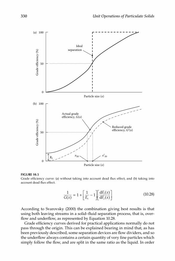
330 Unit Operations of Particulate Solids
1( ) 1
11
d ( )d ( )t
f
G x EF xF x= + −
c
(10.28)
According to Svarovsky (2000) the combination giving best results is that using both leaving streams in a solid–fluid separation process, that is, over-flow and underflow, as represented by Equation 10.28.
Grade efficiency curves derived for practical applications normally do not pass through the origin. This can be explained bearing in mind that, as has been previously described, some separation devices are flow dividers, and so the underflow always contains a certain quantity of very fine particles which simply follow the flow, and are split in the same ratio as the liquid. In order
Particle size (x)
Particle size (x)
Gra
de ef
ficie
ncy (
%)
0
100
50
Rf
Reduced grade efficiency, G′(x)
Actual gradeefficiency, G(x)
x50 x′50
Gra
de ef
ficie
ncy (
%)
50
100(a)
(b)
0
Idealseparation
Figure 10.5Grade efficiency curve: (a) without taking into account dead flux effect, and (b) taking into account dead flux effect.

Solid–Fluid Systems 331
to account for the partition effect (also called “dead flux”) of some solid–fluid separators, the reduced grade efficiency, similar to the reduced efficiency represented by Equation 10.17, can then be obtained as
G x
G x RR
’( )( )= −
−f
f1 (10.29)
As can be seen in Figure 10.5b, the correspondent curve to this definition does cross the origin.
Solid–fluid separators are among those equipments whose separation per-formance is highly dependent on particle size. Thus, according to this, an overall efficiency of separation is not the best way to evaluate their perfor-mance. For this reason, it is advisable to express their efficiency for each size of particle in the range measured. As experience has shown, the only single num-ber, which in some way gives the separation power of a solid–fluid separator, is the cut size. This cut size or cut point (xc, x50) is the particle size at which the grade efficiency curve shows a value of 50%. In other words, particle with such a size will have a probability of 50% of being separated or, most practically, all particles above the cut size will be generally going to the underflow, whereas those below the cut size will be normally reported to the overflow.
As can be concluded, the cut size is derived from a grade efficiency curve. As the calculation and plotting of a full grade efficiency curve is a time con-suming task, alternative ways of determining the cut size have been pro-posed (Trawinski, 1976, 1977). The main drawback of these methods is the need of plotting limited data, and so the advantageous feature is greatly reduced. On the other hand, depending on specific applications, empirical equations of regression models can be consulted to have a rough estimate of cut size in defined equipment units. Doheim et al. (1985), for example, pres-ent a model for prediction of cut size in hydrocyclones using empirical equations.
The sharpness of separation can be related to the shape of the curve in a number of manners. Knowing the grade efficiency curve, comparisons of classification sharpness of different equipments can be made by plotting G(x) against dimensionless size relation x/x50, and comparing the resultant normalized curves. To define the curve steepness, a ratio of two sizes corre-sponding to two different percentages on the grade efficiency curve on either side, and 50% equidistant, can be used. This parameter is called the sharpness index and is represented by
H
xx25/75 =
25
75 (10.30)
It was previously stated that the grade efficiency curve does not go through the origin. The cut size as has been defined is derived from this curve.

332 Unit Operations of Particulate Solids
If, in order to practically assess the performance of solid–fluid separators, a reduced grade efficiency curve is used, the particle size which gives 50% effi-ciency in such a curve is called the reduced cut size and is represented by x50
′ .The maximum attainable efficiency related to particle size would be that
minimum particle size with 100% probability of being reported to the under-flow. Graphically, by extrapolating the end part of the curve to the horizontal axis, such size will be obtained. It has been proved that in practice, the maxi-mum of the efficiency is around 98%, and the minimum size corresponding to this efficiency is represented by x98 and known as the approximate limit of separation.
As a final note is important to bear in mind that solid–fluid separations are governed by mechanical forces, such as the gravity force, and so it is impor-tant that the screen analysis data on the relevant streams used to derive a grade efficiency curve had been measured avoiding transformations. The use of a particle sizer that measures the relevant particle size directly, that is, any method measuring directly the Stokes diameter xst, should be preferred over a method relying on transforming size distributions from number to surface, or surface to mass, and so on.
example 10.2
A hydrocyclone, 44 mm in diameter, is used to separate a suspension of limestone in water. The density of the limestone is 2885 kg/m3 and the gravimetric sepa-ration efficiency was 28.34% while the partition coefficient was determined as 11.62%. Derive a grade efficiency curve to find out the reduced cut size, from the data given in Table 10.2.
Table 10.2
Example 10.2
Particle Size (μm) Fc (%) Ff (%)
15 20.06 69.3520 25.62 79.7325 31.51 86.8130 37.60 91.5735 43.75 94.7240 49.83 96.7745 55.73 98.0850 61.35 98.8955 66.63 99.3860 71.50 99.6765 75.92 99.8370 79.88 99.9275 83.38 99.9680 86.42 99.98

Solid–Fluid Systems 333
SoluTion
Table 10.2 presents the particle size distributions for the overflow and underflow through the hydrocyclone. Therefore, Equation 10.28 would be the appropriate to derive the grade efficiency. Since the separation was carried out in a hydro-cyclone, and this type of device normally presents a dead flux effect previously described, Equation 10.29 should be used to derive the reduced grade efficiency. Carrying out the proper computations using the tabulated data and the equations mentioned, Table 10.3 is obtained.
Plotting the data in Table 10.3, the following graph (see Figure 10.6) can be drawn.
Finally, taking the reading from the above graph in the 50% point of the G′(x) axis an approximate reduced cut size x50
′ = 40 μm is obtained.
10.3 Solid–Gas Separations
10.3.1 introduction
Two-phase systems of fine dispersed solids in a continuous gas stream are quite common in many processing industries dealing with dry solids opera-tions. In diverse processes such as the dry milling of grains, some combustion reactions, or the grinding of raw materials in the cement industry, fine solids may be released to the surrounding air as part of their normal operation. Tiny solid particles (dust) produced in many processes may become airborne and carried out by air currents. There are many problems associated with dust emissions, such as health hazards, abrasion damage to equipment, impaired
Table 10.3
Example 10.2
Particle Size (μm) G(x) (%) G′(x) (%)
15 12.92 2.6820 18.87 9.3325 26.42 17.7730 35.44 27.8535 45.54 39.1340 56.02 50.8545 66.09 62.1050 75.05 72.1255 82.47 80.4160 88.23 86.8465 92.44 91.5570 95.36 94.8275 97.29 96.9880 98.51 98.33

334 Unit Operations of Particulate Solids
visibility, unpleasant odors, material loss, and risk of dust explosions. Another common situation of two-phase (solid–gas) system is when such system results from a specific operation, like in pneumatic conveying or in spray drying. In all these described cases, it becomes necessary to separate the dispersed or suspended solids from the airstream (or any other gas).
Two types of solids dispersoids causing problems in diverse processes have been recognized: dust consisting on particles larger than 1 μm, and fume formed by particles smaller than 1 μm. Fumes are also defined as par-ticles that, once settled, do not normally return to an airstream, while dusts can be considered particles that even after settling may become airborne again as an effect of an air draft or blast.
A number of solid–gas separation techniques, such as cyclonic separation, gas filtration, or scrubbing, can be used to purify dust-laden gases or recover particulate solids from streams carrying them.
10.3.2 use of Cyclones
An inert force commonly employed in separating solids particles from a gas stream is the centrifugal force. Cyclones and air classifiers represent tech-niques that make use centrifugal force as a means of performing separation. Air classification may be considered an analytical technique with some industrial applications, while cyclonic separation constitutes one of the most useful industrial operations to treat dust-laden air and gases in a number of processes and applications.
10.3.2.1 Description of the Process
Cyclones are by far the most common type of gas–solids separation device used in diverse industrial processes. They have no moving parts, are
0102030405060708090
100
0 10 20 30 40 50 60 70 80 90Equivalent stokes diameter (μm)
Gra
de ef
ficien
cy (%
)G(x)G′(x)
Figure 10.6Example 10.2.

Solid–Fluid Systems 335
inexpensive compared to other separation devices, can be used at high tem-peratures, produce a dry product, have low energy consumption, and are extremely reliable. Cyclone operation obeys fundamental physical laws and there are certain limitations in particle size to be successfully captured in a given unit. However, high-efficiency cyclones can be designed to collect a great proportion of any industrial dust, down to the smaller particle sizes and approaching the borderline between dust and fumes.
As illustrated in Figure 10.7, a cyclone consists of a vertical cylinder with a conical bottom, a tangential inlet near the top, and outlets at the top and the bottom, respectively. The top outlet pipe protrudes into the conical part of the cyclone in order to produce a vortex when a dust-laden gas (normally air) is pumped tangentially into the cyclone body. Such a vortex develops centrifu-gal force and, because the particles are much denser than the gas, they are projected outward to the wall flowing downward in a thin layer along this in a helical path. They are eventually collected at the bottom of the cyclone and separated. The inlet gas stream flows downward in an annular vortex, reverses itself as it finds a reduction in the rotation space due to the conical shape, creates an upward inner vortex in the center of the cyclone, and then exits through the top of the cyclone. In an ideal operation in the upward flow
Dust discharge
Feed
Gas outlet
Figure 10.7Schematic diagram of a cyclone.

336 Unit Operations of Particulate Solids
there is only gas while in the downward flow there are all the particles fed with the stream. Cyclone diameters range in size from less than 0.05 m to 10 m, feed concentrations cover values from 0.1 kg/m3 to approximately 50 kg/m3, while gas inlet velocities may be in the order of 15–35 m/s.
10.3.2.2 Theoretical Aspects
A cyclone is in fact a settling device in which a strong centrifugal force, acting radially, operates instead of the relatively weak gravity force, acting vertically. Due to the small range of particles involved in cyclone separation (the smallest particle that can be separated is about 5 μm), it is considered that Stokes law primarily governs the settling process. Substituting, thus, the expression for centrifugal acceleration g = ω2r into Equation 10.11, the resul-tant equation is
v
x rr
2s g( )18
=−ρ ρ ω
µ
2
g (10.31)
where vr is the terminal velocity of the particle covering the radius r, x is the equivalent particle diameter, ρs the density of the particle, ρg the density of the gas, and μg the viscosity of the gas.
Also, the centrifugal acceleration is a function of the tangential component of the velocity according to the following expression:
ω = v
rtan
(10.32)
where vtan is the tangential velocity of the particle in the radius r. Substituting Equation 10.32 into Equation 10.31:
v
x vrr
s g
g=
−2 2
18( ) tanρ ρ
µ (10.33)
Multiplying Equation 10.33 by g/g, the resultant equation gives
v
x g vgr
uvgrtt
s g
g=
−
=
2 2 2
18( )
( )tan tanρ ρµ
(10.34)
where ut is the terminal settling velocity defined by Equation 10.11. As can be implied, and according to Equation 10.34, the higher the terminal velocity, the easier it is to “settle” a particle within a cyclone.

Solid–Fluid Systems 337
10.3.2.3 Operating Variables
For a given particle size, the terminal velocity is a maximum in the inner vortex, where r is small, so that the finest particles separated from the gas are eliminated in the inner vortex. These particles migrate through the outer vortex to the wall of the cyclone and drop passing the bottom outlet. Smaller particles that do not have time to reach the wall are retained by the air, and carried to the top outlet. Although the chance of a particle for sepa-ration decreases with the square of the particle diameter, the fate of a par-ticle depends also on its position in the cross section of the entering stream and on its trajectory in the cyclone. Thus, the separation according to size is not sharp. For cyclones the cut diameter or cut size, can be defined as that diameter for which one-half of the inlet particles, by mass, are separated while the other half are retained by the gas. The cut size is a very useful variable to determine separation efficiency of a cyclone. Since a given pow-der to be separated in a cyclone would have an extremely fine half of its distribution, such half may not be easily separated using conventional pressure drops. Therefore, it is advisable to make it the cut size to coincide with the mean size of a powder particle size distribution to guarantee sepa-ration of the coarse part of such distribution, as the fine one may unattain-able due to the small range involved. According to this criterion, the cut size would represent the size to be captured inside the cyclone to guaran-tee a 50% collection of the fed particles. Substituting such size in Equation 10.34 would fix a velocity to carry out the desired separation. Since in prac-tice evaluation of radial velocity is difficult as it depends on the terminal gravitational velocity, the tangential velocity, and the radial and axial position of the cyclone, empirical relations alternative to Equation 10.34 have been suggested. An alternative equation that has been used for this purpose is the following:
v
x brnt
2s g( )
18=
−ρ ρµ
1
g (10.35)
where b1 and n are empirical constants.Experience and theory have shown that there are certain relationships
among cyclones dimensions that should be observed for efficient cyclone performance (Geldart, 1986), and which are generally related to the cyclone diameter. There are several different standard cyclone “designs” and a very common is called the “Stairmand” design, whose dimensions are shown in Figure 10.8. Using standard geometries of cyclones is much easier to predict effects on variables changes and scale-up calculations are greatly reduced. Such calculations may be carried out by means of dimensionless relation-ships. Selection and operation of cyclones can be described by the relation-ship between the pressure drop and the flow rate, and the relationship

338 Unit Operations of Particulate Solids
between separation efficiency and flow rate (Svarovsky, 1981). The funda-mental equations to apply the dimensionless scale-up model are
Eu
2g
= =∆Pv
kρ 2
(10.36)
Stk
41850
502
s
g c3= =Qx
Dk
ρµ π
(10.37)
where Eu is the Euler number for a given pressure drop ΔP of a gas of density ρg flowing through the cyclone at a velocity v. Stk50 is the Stokes number for a cut size x50 of a solid of density ρs suspended in a gas of viscosity μg passing through the cyclone of diameter Dc at a volumetric flow rate Q. The cyclone body velocity v is the characteristic velocity that can be defined in various
0.5 Dc
0.5 Dc0.5 Dc
1.5 Dc
2.5 Dc
Dc/3
Dc
Figure 10.8Dimensions of standard Stairmand cyclone.

Solid–Fluid Systems 339
ways, but the simplest one is based on the cross section of the cylindrical body so that
v
QD
= 4π c
2
(10.38)
As can be implied by inspecting Equations 10.36 through 10.38, for given values of ΔP, ρs, ρg, and μg: X50 ~ (Dc)0.5, whereas for a given value of X50: ΔP ~ (Q)2/3; ΔP ~ (Dc)2; and Q ~ (Dc)3.
When designing cyclone systems, it is essential for optimum results to have full process data available, as there are a number of variable factors that will determine the final performance.
Cyclone inlet velocity not only affects efficiency of separation but also reflects in pressure loss and possible erosion. Gas viscosity has an important effect on particle efficiency, and so it is advisable to check its dependency with temperature and consider those cases in which a gas different from air is involved in the process. Smaller cyclone diameters increase overall efficiency, but also promote erosion. In addition to this, it is sometimes necessary to con-sider possible attrition of solids in the cyclone, which will result in production of fines and considerable losses. Erosion occurs primarily where the particles first impact the cyclone wall, but also occur at the bottom of cyclones too short to accommodate the length of the naturally occurring vortex.
In order to remove as much as the dust from a gas stream as possible, cyclones are often placed in series with each other to increase the overall col-lection efficiency relative to a single unit. Although this is theoretically true, the efficiency is increased at the expense of pressure drop, and so extreme care should be taken to consider whether great efficiency will render a costly process. There is also a great complexity when trying to improve collection efficiency using many small cyclones in parallel to replace a large cyclone. A disadvantage of parallel cyclones is that equal gas distribution to each cyclone can be difficult to achieve. If this occurs, collection efficiency is reduced with the advantages of parallel cyclones being greatly negated.
There is an increasing trend toward using cyclones for final cleaning for environmental purposes in processes where it is becoming economically impractical to use other methods. There are many applications where this can be done subject to certain limitations, by the use of one, two, or even three stages of separation. In many cases a first-stage cyclone can be used to deal with high inlet loadings and will produce excellent results at the expense of reasonable pressure loss. The addition of a second stage to deal with the first-stage losses can then often achieve required results, but where further cleaning is necessary a third-stage cyclone may provide the answer. The use of a third-stage cyclone invariably means that a high degree of clean-up is necessary and, therefore, the third stage should give the best possible efficiency and be capable of maintaining this efficiency for a long time. The use of several stages to try to improve efficiency or remove very fines particles

340 Unit Operations of Particulate Solids
may become impractical by employing only cyclones. This difficulty can be alleviated by combining methods so that, for environmental purposes when certain particles need to be removed regardless of their fineness, bag filters may be coupled with cyclones.
10.3.2.4 Applications
As mentioned before, cyclones are extensively used in the processing indus-try to reduce particle load to safe levels in dry milling, as well as in classifica-tion of particles in closed-circuit grinding operations. They are also employed in recovering fines from spray drying and fluidized bed drying processes. Another important application is in pneumatic conveying of diverse food products, such as grains and flours.
example 9.3
Calculate the cut size for particles suspended in air and treated in a cyclone 1.48 m in diameter operating at a pressure drop of 1200 Pa. The density of the particles id 2.6 g/cm3, the density of the suspending air is 1.2 kg/m3, while its viscosity is 1.825 × 10⁻⁵ N s/m2. The pressure drop coefficient is 320 and the Stokes number is 0.00012.
SoluTion
As can be deducted, the pressure drop coefficient refers to the Euler number. Substituting, thus, Equation 10.38 into Equation 10.36 and transposing for Q, and substituting values on the resulting equation, that is,
Q
P D m m= = =∆ πρ
π2c4
g
2 4
38 Eukg/s
kg/m
( ) ( ) ( . )( . ) ( )
1200 1 488 1 2 320
2 4
44 3 m /s3.
Using the above flow rate, and transposing for the cut size in Equation 10.37, it is substituted along with the other values to obtain the cut size as
x
DQ
50
5184
0 0001218 1 825 10 1 48= = × −Stk kg/ms50 c3
s
( ) . ( )( . ) ( ) .µπρ
π 33
4 4 3 2600m
m /s kg/m
3
3 3( . ) ( )
The cut size is, therefore: x50 = 2.99 × 10⁻⁶ m ~ 3 μm.
10.3.3 air Classifiers
10.3.3.1 Description of the Technique
Air classification is a method of separating powdery, granular, or fibrous materials in accordance with the settling velocity and combined with the

Solid–Fluid Systems 341
influence of particle size, particle density, and particle shape. The procedure of winnowing or aspiration is a traditional way of separating chaff from grain after threshing and is one of the simplest forms of air classification. Ideally, the separation effect of an air classifier should be such that all parti-cles that exceed the cut point are transported into the coarse fraction and the smaller particles are transported to the fines fraction. In this sense, air clas-sification basically consists of dividing particle size distributions of given powders and, as such, is a technique commonly used in combination with size reduction equipment, normally to eliminate fines that may affect prop-erties like wettability and dispersibility. The major interest in air classifica-tion is that it provides a means for separating small particles, in a dry manner, which cannot be readily achieved by sieving, that is, below 50 μm. Ortega-Rivas and Svarovsky (2000) report a successful sharp split of the particle size distribution of calcium carbonate, into a fine fraction with mean particle size as fine as 6 μm.
10.3.3.2 Theoretical Aspects
The mode of operation of a typical air classifier is as follows. The inlet air is mixed with the material being separated. The feed particles are subjected to a centrifugal force operating from a revolving rotor and a drag force pro-duced by the air current, which moves in a spiral direction toward the cen-tral shaft. As previously mentioned, the separation is based on differential mass, density, and shape. The larger and more dense particles are influenced by the mass-dependent centrifugal forces and move toward the outside of the chamber, where they are removed by a screw conveyor or some alterna-tive means. The smaller, lighter particles are more subjected to the frictional forces of the air current moving, therefore, with the airstream and leaving from the center of the classifying chamber to be separated by a cyclone from the airstream. The relative magnitude of these two forces can be changed by altering the rotational speed of the disc and the air velocity. By varying either of these, there will be an effect on the cut size. A common design of air clas-sifier consists of a rotating wheel with zigzag channels over its surface, each of them comprising six components. A diagram of this type of classifier is shown in Figure 10.9.
Classifiers with the facility to change rotational speed and air velocity independently will be very flexible in operating terms. Although the separa-tion mainly takes place within the classifying chamber, some preliminary removal of the coarsest particles may be achieved outside the chamber. The disc or turbine can be mounted on a horizontal or vertical axis. The latter produces a centrifugal force in the horizontal plane, favoring high through-puts but low precision in cut size (Fedoc, 1993). Air classifiers are categorized by reference to a number of factors such as the presence or absence of a rotor, the drag force on the air, the relative velocity and direction of the air and particles, the use of directional devices such as vanes or cones, and the

342 Unit Operations of Particulate Solids
location of the fan and fines collection devices. Other important features include the capacity of the classifier and the energy utilization. A comprehen-sive treatise of classifier types has been presented by Klumpar et al. (1986).
The obvious method of characterization of separation capability of air clas-sifiers is by using the cut size concept. Ideally, all particles below the cut size would end up in the fines stream while all particles above the cut size would follow the coarse stream. However, there will be always misplaced material, that is, a small fraction of particles smaller than the cut size would be in the coarse stream and an equally small proportion of particles larger than the cut size would appear in the fines stream. The extent of the overlap due to misplaced material, as well as the cut size, can be determined by measuring the particle size distributions of both streams, and presenting their data as a weight frequency distribution. The yields of fines Yf and coarse Yc streams need to be identified. When they are equal, the point of overlap gives the cut size. When they are not equal, which is most likely, the frequency distribution for the fines stream must be multiplied by the yield for the fines stream, while the yield for the coarse stream must be multiplied by the yield for the coarse stream. The cut size is, thus, given by the point of intersection of these curves.
In air classifiers a solid-state element in a rotor is radially affected by two forces: a centrifugal force toward the outside and the frictional force of the air toward the inside. Since particles quite fine are of interest, assuming
Classifyingair
Fineproduct
Driveshaft
Dosingscrew
Feed
Classifierwheel
Classifying air
Coarseproduct
Figure 10.9Diagram of an air classifier.

Solid–Fluid Systems 343
Stokes law applicability, the resulting equilibrium between the two men-tioned forces for a certain grain size would be the so-called cut size. Particles larger than the cut size are centrifugally extracted as oversized toward the outside, while smaller particles are carried inside by the airstream. Assuming a constant air throughput, the fineness of the separation in the classifier depends on the peripheral speed of the particle, which in turn is in confor-mity with the peripheral speed of the rotating wheel. With the speed remain-ing constant, an increasing air throughput changes the cut point within the coarser range. In principle, any cut point can be attained by combining two matching values of speed and air throughput.
By equating the above-mentioned forces when they are in equilibrium, a relation for the cut size x50 based on Stokes law can be derived as follows:
x
v rv
t502
2
18=
−µρ ρ
g
s g( )tan (10.39)
where vt is the radial speed of air, r is the radius of the classifier wheel, and vtan is the peripheral speed of particle. Equation 10.39 is useful in predicting how airflow and rotational speed may influence the cut size. Basically, it pre-dicts that increasing the airflow rate would increase the cut size, whereas increasing the rotational speed would decrease this cut size.
10.3.3 operation and applications
Due to the complicated flow conditions in air classifiers, the classifying results with the given values of speed and air throughputs cannot be prede-termined. For this reason, the assignment of cut point and operating data of the classifier are determined by experiments with a calibration curve. The various particle sizes of a given material of known distribution are used to plot the calibration plot. These particle sizes are separated under certain con-ditions of speed and air throughput. The coarse fraction is weighed at the same time. The particle size corresponding to the coarse grain proportion and legible from the fineness characteristics is the cut point according to the operating conditions of the individual classifier, also known as analytical cut point. For inert materials with densities of the order of 2600 kg/m3, cut points between 1 and 100 μm are obtained with a “normal” air throughput (0.5–3 kg/h) and by varying the speed between 2500 and 20,000 rpm. Figure 10.10 shows a calibration curve for these variables. Within these ranges, the volumetric flow rate of air V is related to the peripheral velocity N by the following expression:
V
N= −551000
(10.40)
where V is expressed in m3/h and N in rpm.

344 Unit Operations of Particulate Solids
For materials different to the one used for obtaining the graph, if proper-ties are not radically different it can be shown that the equation below will give possibility of evaluating a new cut size:
( )( )
50 1
50 2
2
1
xx
= ρρ
(10.41)
where (x50)1 and ρ1 are the characteristics of the material being evaluated, while (x50)2 and ρ2 correspond to the calibration curve material (calcium car-bonate for Figure 10.10).
Air classification is used in a number of industries in important applica-tions. For example, it is used in the pharmaceutical industry to determine the absorbing capacity of drugs and active substances, which is a function of their fineness. In grain processing, an application is the wheat flour fraction-ation to separate the coarse, low protein fraction, from the fine, high protein fraction. Other food-related applications include classification of confection-ery products, soy flour, potato granules, rice flour, lactose, and oleaginous fruits, removal of shells or hulls from disintegrated peanuts, cottonseed, rapeseed, or cocoa beans, preparation of oat-bran, and separation of gossypol from cottonseed protein. Air classifiers are widely used in many comminu-tion processes in the mining, chemical, and other types of industries, for separation of specific fraction for diverse purposes and applications.
Cut s
ize (
μm)
100
50
10
5
11000 5000 10,000 50,000
Rotor speed (rpm)
Figure 10.10Calibration curve for an air classifier.

Solid–Fluid Systems 345
10.3.4 gas Filters
10.3.4.1 Description of the Process
Gas–solids separations can be performed using filtration means. Gas filters are used for final particulate removal in many processes of the chemical and related industries. These filters can capture particles much smaller in diameter than a cyclone so they are commonly placed downstream of a cyclone in diverse applications. A gas filter generally consists of a porous fabric, which can be woven to conform to the shape of a cylinder or may be supported in a frame. The former is called a bag filter while the latter is known as an envelope filter. The main difference of both designs is in the way solids are accumulated. In bag filters dust may accumulate inside, whereas in envelope filters it would form a cake outside. The filtering arrangements are placed in a matrix so that their total area will result in a low gas velocity through the bags and, therefore, a low pressure drop through the filter. Gas velocities through the filtering media are of the order of 0.005–0.02 m/s. Particulate loadings to these filters generally lie in the range of 0.2–250 g/cm3. Diagram of the two main types of gas filters are given in Figures 10.11 and 10.12. Filters used in gas–solids separations may be woven or felted fabrics of natural or synthetic fibers. There are tables list-ing properties of filtering media to determine whether they are suitable for applications at diverse conditions, such as high temperatures, corrosive and chemical resistance, and so on (Green and Perry, 2008). Table 10.4 presents properties of some fabrics and fibers used in air filtration, while Table 10.5 gives resistance and permeability factors for some air filtration fabrics.
Solids out
Air
Reverse flow Clean air
Feed
Filtering elements
Filtration cycle Cleaning cycle
Figure 10.11Bag filter with internal accumulation of solids.
346 Unit Operations of Particulate Solids
Filtrations may also be made with granular solids in the form of stationary or moving beds. Many other types of materials porous in nature, or capable of providing a screening effect after weaving or fabrication, may be found suitable for certain filtration applications.
In gas filtration, the collected particles build up on the surface of the filter-ing medium and cause a gradual increase in the pressure drop through the
Clean air
Feed
Solids out
Envelope
Figure 10.12Bag filter with external accumulation of solids.
Table 10.4
Physical Properties of Some Fabrics and Fibers Used in Air Filtration
FiberWeight (g/m2)
Thickness (mm)
Rupture Force
(N/mm)
Elongation (% to
Rupture)
Air Permeability [(m3/s)/m2 a
Δpf = 0.12 kPa] Kc
Wool 859.3 3.43 0.138 1.03Wool 788.7 3.28 0.151 0.93Orlon 405.5 1.14 11.38 18 0.102–0.127 1.11–1.39Orlon 665.9 2.24 14.89 18 0.076–0.102 1.39–1.85Orlon 892.8 3.18 19.26 60 0.051–0.102 1.39–2.78Acrylic 665.9 1.91 17.51 22 0.076–0.102 1.39–1.85Dynel 892.8 3.18 10.51 80 0.152–0.203 0.70–0.93Dacron 665.9 2.03 21.89 22 0.076–0.102 1.39–1.85Dacron 368.3 6.35 3.50 150 1.016–1.143 0.11–0.14Dacron 892.8 3.18 30.65 80 0.102–0.152 0.93–1.39Nylon 892.8 3.18 17.51 100 0.152–0.203 0.70–0.93Arnel 892.8 3.18 10.51 80 0.152–0.203 0.70–0.93Teflon 580.3 1.35 0.419 0.34
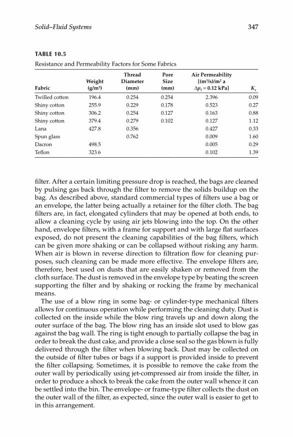
Solid–Fluid Systems 347
filter. After a certain limiting pressure drop is reached, the bags are cleaned by pulsing gas back through the filter to remove the solids buildup on the bag. As described above, standard commercial types of filters use a bag or an envelope, the latter being actually a retainer for the filter cloth. The bag filters are, in fact, elongated cylinders that may be opened at both ends, to allow a cleaning cycle by using air jets blowing into the top. On the other hand, envelope filters, with a frame for support and with large flat surfaces exposed, do not present the cleaning capabilities of the bag filters, which can be given more shaking or can be collapsed without risking any harm. When air is blown in reverse direction to filtration flow for cleaning pur-poses, such cleaning can be made more effective. The envelope filters are, therefore, best used on dusts that are easily shaken or removed from the cloth surface. The dust is removed in the envelope type by beating the screen supporting the filter and by shaking or rocking the frame by mechanical means.
The use of a blow ring in some bag- or cylinder-type mechanical filters allows for continuous operation while performing the cleaning duty. Dust is collected on the inside while the blow ring travels up and down along the outer surface of the bag. The blow ring has an inside slot used to blow gas against the bag wall. The ring is tight enough to partially collapse the bag in order to break the dust cake, and provide a close seal so the gas blown is fully delivered through the filter when blowing back. Dust may be collected on the outside of filter tubes or bags if a support is provided inside to prevent the filter collapsing. Sometimes, it is possible to remove the cake from the outer wall by periodically using jet-compressed air from inside the filter, in order to produce a shock to break the cake from the outer wall whence it can be settled into the bin. The envelope- or frame-type filter collects the dust on the outer wall of the filter, as expected, since the outer wall is easier to get to in this arrangement.
Table 10.5
Resistance and Permeability Factors for Some Fabrics
FabricWeight (g/m2)
Thread Diameter
(mm)
Pore Size (mm)
Air Permeability [(m3/s)/m2 a
Δpf = 0.12 kPa] Kc
Twilled cotton 196.4 0.254 0.254 2.396 0.09Shiny cotton 255.9 0.229 0.178 0.523 0.27Shiny cotton 306.2 0.254 0.127 0.163 0.88Shiny cotton 379.4 0.279 0.102 0.127 1.12Lana 427.8 0.356 0.427 0.33Spun glass 0.762 0.009 1.60Dacron 498.5 0.005 0.29Teflon 323.6 0.102 1.39
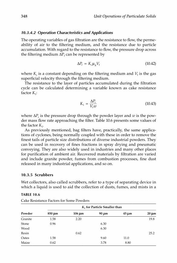
348 Unit Operations of Particulate Solids
10.3.4.2 Operation Characteristics and Applications
The operating variables of gas filtration are the resistance to flow, the perme-ability of air to the filtering medium, and the resistance due to particle accumulation. With regard to the resistance to flow, the pressure drop across the filtering medium ΔPf can be represented by
∆P K Vf c g f= µ (10.42)
where Kc is a constant depending on the filtering medium and Vf is the gas superficial velocity through the filtering medium.
The resistance to the layer of particles accumulated during the filtration cycle can be calculated determining a variable known as cake resistance factor K1:
K
PV w1 = ∆ c
f (10.43)
where ΔPc is the pressure drop through the powder layer and w is the pow-der mass flow rate approaching the filter. Table 10.6 presents some values of the factor K1.
As previously mentioned, bag filters have, practically, the same applica-tions of cyclones, being normally coupled with these in order to remove the finest tails of particle size distributions of diverse industrial powders. They can be used in recovery of fines fractions in spray drying and pneumatic conveying. They are also widely used in industries and many other places for purification of ambient air. Recovered materials by filtration are varied and include granite powder, fumes from combustion processes, fine dust released in many industrial applications, and so on.
10.3.5 Scrubbers
Wet collectors, also called scrubbers, refer to a type of separating device in which a liquid is used to aid the collection of dusts, fumes, and mists in a
Table 10.6
Cake Resistance Factors for Some Powders
Powder
K1 for Particle Smaller than
850 μm 106 μm 90 μm 45 μm 20 μm
Granite 1.58 2.20 19.8Stone 0.96 6.30Wood 6.30Resin 0.62 25.2Oates 1.58 9.60 11.0Maize 0.62 3.78 8.80
Solid–Fluid Systems 349
number of industrial operations. There are numerous designs of scrubbers commercially available that have been devised over the years, but they operate basically on the same principle in which solid particles may be often scrubbed from a gas stream by spraying a jet of a liquid, usually water, into that stream. Depending on their design and operating condi-tions, particle scrubbers can be adapted to collect fine or coarse particles that are intercepted by the droplets of the water spray and are removed by the scrubber in the form of slurry. The predominant mechanism of particle entrapment by the liquid appears to be inertial deposition. Flow-line inter-ception is only a minor mechanism in the collection of the finer dust par-ticles by liquid droplets of the sizes encountered in scrubbers. Diffusion is indicated to be a relatively minor mechanism for the particles larger than 0.1 μm that are of principal concern. Although scrubbers are normally more efficient than cyclones, they have the disadvantage of collecting the solids wet instead of dry. If this feature is unacceptable or impractical for processing reasons, the solids must be separated from the liquid. In such a way, the gas–solids collection problem would be replaced by a solid–liquid separation difficulty.
10.3.5.1 Process Description
The predominant separation mechanism in scrubbing is impact due to the inertia of a particle with density relatively higher than that of the liquid. In such a way, the relative velocity between the particle and the liquid droplet is an important factor and the process may depend on the acceleration of, both, the particle and the droplet in relation to the point of impact. The process may be controlled by varying the droplet velocity, in order for the particle to collapse with it. The efficiency of the scrubbers is normally expressed as the fraction of particles collected from a volume of gas, deter-mined by the projected area of the receiving body. To achieve this, a separation number Se (Maas, 1979), may be defined as
Se t
L b= u V
g D0
(10.44)
where ut is the Stokes terminal velocity, V0 is the mean gas velocity, gL is the local gravity acceleration, and Db is the liquid droplet diameter. The effi-ciency of separation η can be correlated to the separation number Se using graphs like the one shown in Figure 10.13.
10.3.5.2 Equipment and Applications
A typical device, known as spray cyclonic scrubber, consists on a cylindrical chamber with a conical bottom as illustrated in Figure 10.14. The scrubber

350 Unit Operations of Particulate Solids
operation is countercurrent with the feed entering by a tangential port at the bottom and traveling upward through a water layer formed by the spray fall-ing on the swirl vanes mounted on paddles. After the gas current passes through the water layers toward the internal center of the vanes, it changes direction crossing the paddles. An upper vane is used to separate the
0.001 0.1 1.0 10 100
0.2
0.8
1.0
0.4
0.6
0
Separation number (Se)
Effic
ienc
y (η)
Figure 10.13Efficiency of separation versus separation number for spherical droplets in scrubbers.
Feed air
Washingwater
Clean air
Washing water
Swirl vanes
Paddles
Dragseparator
Figure 10.14Diagram of spray cyclone scrubber.

Solid–Fluid Systems 351
remaining droplets and allow the air to come out clean from the top outlet, as shown in Figure 10.14. This equipment combines the cyclonic action with the scrubbing of the liquid.
Other types of equipment used for scrubbing include plate towers, self-induced spray scrubbers, venturi scrubbers, mechanical scrubbers, and fiber-bed scrubbers. The principle of operation of all these units is, practically, similar. Their operating principles can be consulted in reference textbooks (Green and Perry, 2008).
Gas scrubbers have the same sort of applications of the previously described solid–gas separators. They are particularly useful in the separation of fumes from combustion reactions and to eliminate mists in production of different acids in many industrial processes.
10.3.6 other Techniques
10.3.6.1 Settling Chambers
Gravity collectors are generally built in the form of long, empty, horizontal, rectangular chambers with an inlet at one end and an outlet at the side or top of the other end (Figure 10.15). Inside that chamber the gas velocity is reduced to enable dust to settle out by the action of gravity. Its simplicity lends it to almost any type of construction. Practically, however, its industrial utility is limited to removing particles larger than 43 mm diameter. For removing smaller particles, the required chamber size is generally excessive. By assum-ing a low degree of turbulence relative to the settling velocity of the dust particle in question, the performance of a gravity settling chamber expressed as efficiency of separation η may be given by
η = u L
H Vt s
s s (10.45)
Feed
Clean air
Settledparticles
Figure 10.15Dust-settling chamber.
352 Unit Operations of Particulate Solids
where ut is the terminal settling velocity of the particle, Ls is the length of the chamber, Hs is the height of the chamber, and Vs is the superficial velocity of the gas through the chamber.
Since the pressure drop through a settling chamber is small, and because low gas velocities are used, the chamber is not subject to abrasion and may therefore be used as a precleaner to remove very coarse particles and thus minimize abrasion on subsequent equipment.
10.3.6.2 Electrostatic Separators
This type of equipment separate solids, or liquids, from a gas stream by pass-ing it through a strong, high-voltage field produced between two electrodes of opposite polarity. The field imposes a charge on the particles so that they migrate toward the collecting electrode. The particles are usually removed from the electrode by periodic rapping. The advantage of an electrostatic precipitator is that it can collect solids of very small size in a dry form. Electrostatic precipitators are generally large units of equipment, because collection efficiency is proportional to the area of the collecting electrodes. For this reason, capital costs are very high, although operating costs are low and may justify the use of a precipitator instead of a filter for some particular applications (Svarovsky, 1981).
Electrostatic separators can be selected according to the following funda-mental equation:
η = − −1 e ( )w A / V (10.46)
where η is the efficiency of separation, w is the migration velocity, A is the area of the collecting electrodes, and V is the volumetric flow rate of gas.
Theoretically, the migration velocity w can be evaluated from
w
aE E= 0 p
6πµg (10.47)
where a is the radius of the dust particle, E0 is the strength of the electrical field where the particle is charged, Ep is the strength of the field in the set-tling point, and μg is the gas viscosity.
Electrostatic precipitators have been used successfully to eliminate fine dusts in many types of waste gases. They have been employed in settling of fine powders of lead oxide, arsenic, and foundry gases. Other applications include settling of dust from gases produced in cement ovens, and in the recovery phosphorous pentoxide from gases produced in phosphorous ovens.

Solid–Fluid Systems 353
10.4 Solid–Liquid Separation Techniques
As previously mentioned, solid–liquid separations constitute an important number of operations in diverse processing industries. Solid–liquid separation is an important industrial process used for recovery of solids from suspen-sions and/or purification of liquids. Dense, concentrated, and dilute suspen-sions handled in many of these industries need to be depurated or purified by separating phases, and the desired product can be the clarified liquid or the dried solid. The different theoretical aspects needed to understand the operat-ing principles of all the mechanical operations employed in separating compo-nents in two-phase and multiphase systems can be facilitated by, first, dealing with the general aspects of properties of suspensions. Properties and pretreat-ment of suspensions will be studied in the first part of this section, prior to get involved in the study if the different solid–liquid separation techniques. Many slurries and suspensions treated in the materials processing industry behave as non-Newtonian liquids but the current theory describing the solid–liquid separation process normally applies to Newtonian suspensions only. The reviewing part dealing with properties of suspensions will therefore include a component dealing with non-Newtonian suspensions.
10.4.1 Properties of Suspensions: rheology and Flow
The rheological properties of suspension have been studied since the begin-ning of last century. The first research was done by Einstein (1906, 1911), in his classical study of the viscosity of dilute suspension of rigid spheres. His approach is purely hydrodynamic, and his model consists of an isolated sphere situated in a simple shear flow field in an infinite fluid. A number of workers have been extending Einstein’s analysis (Frisch and Simha, 1956). Three approa ches have been presented: the theoretical basis of viscosity com-putation, the effect of particle texture and shape, and the effect of concentra-tion. Some relationships have been developed for correction of viscosity of suspensions in which nearest-neighbor interactions cannot be neglected. Guth and Simha (1936) considered the first-order effect of spheres interacting with one another. They found that
µµo
214.1= + +1 2 5. ø ø
(10.48)
where μ is the viscosity of the suspension, μo is the viscosity of the pure solvent, and ø is the volume fraction of spheres in the suspension. A later correction gave a value of 12.6 for the last constant (Simha, 1952).
For more concentrated systems other approaches have been given. Several authors have made experimental studies of the effects of concentration on the

354 Unit Operations of Particulate Solids
viscosity of suspension of spheres. The data they have proposed are considerably scattered. Thomas (1963) has tried to find the sources of scatter in the data. He found that it is caused in large part by variations in particle size. For small particle sizes (diameters <1–10 μm) colloidal forces become important and the viscosity begins to increase as particle size decreases. The viscosity is also shear rate dependent in this case. For particles larger than 1–10 μm, the particle Reynolds number becomes significant. The inertial effects results in an increase in relative viscosity with increasing particle size. Thomas has developed a unique curve, by eliminating diameter and shear rate effects. For low-concentration data, such a graph can be represented by
µµo
211.4= + +1 2 5. ø ø
(10.49)
Equations 10.48 and 10.49 would be used for correcting the viscosity of concentrated suspensions following a Newtonian behavior.
Many concentrated suspensions follow non-Newtonian behavior and con-siderations ought to be made as the viscosity is not a constant anymore, and such fluids should be characterized properly to use their parameters of charac-terization instead of viscosity in calculations using some dimensionless groups. Most of the theory developed for non-Newtonian fluid flow through tubes, apply to laminar flow round smooth tubes. The most studied non-Newtonian fluids are the power-law fluids and there are some relationships available for pressure-loss-flow rate in purely viscous and viscoelastics flows principally. Relations for thixotropic and rheopectic systems appear not to be available.
Under the assumptions that purely viscous behavior prevails and that no slip occurs at the tube wall, the power-law equation for laminar flow is in the form (Geankoplis, 2003):
τw = =
D PL
Kv
D
n∆4
8’
’
(10.50)
where τw is the shearing stress at the wall of the tube, D is the tube diameter, ΔP is the pressure drop, L is the length of the tube, v the mean velocity, n′ is the slope of the line when the data are plotted on logarithmic coordinates. For n′ = 1, the fluid is Newtonian; for n′ < 1, pseudo plastic, or Bingham plas-tic if the curve does not go through the origin; and for n′ > 1, dilatant. The term K′ is the consistency index; as the name suggest, the larger its value the thicker or more viscous the fluid.
It may be shown (Dodge and Metzner, 1959) that the constant K′ may be related to the analogous power-law constant K (Table 10.1) as follows:
K K
nn
vD
n n n
’’
’
’
= +
−3 14
8
(10.51)

Solid–Fluid Systems 355
if the fluid obeys the power law, n = n′ and
K K
nn
n
’ = +
3 14
(10.51b)
Since Equation 10.50 rigorously portrays the laminar flow behavior of the fluid (provided n′ and K′ are evaluated at the correct shear stress), it may be used to define a Reynolds number applicable to all purely viscous fluids under laminar flow conditions. This dimensionless group can be derived simply by the substitution of (DΔP/4L) from Equation 10.50 into the usual definition of the fanning friction factor, that is,
f
D P Lv
=∆ /
/422ρ
(10.52)
such substitution leads to
f
D vn n= −16
2
γρ’ ’
(10.53)
where γ = K′8n′−1 and all the remaining components as already defined.By letting f = 16/Re as for Newtonian fluids in laminar flow, the above-
mentioned generalized Reynolds number can be obtained as
Re*
’ ’
=−D vn n2 ρ
γ (10.54)
If the equation is desired in terms of K instead of K′, Equation 10.51b may be substituted into Equation 10.54 and
Re* =+( )−
−
D v
K n n
n n
n n
2
18 3 1 4
ρ
(10.55)
For Newtonian fluids n′ = 1 and K′ = μ, so γ reduces to μ and Re* in Equation 10.55 transforms to the familiar Dvρ/μ showing that this traditional dimen-sionless group is merely a special restricted form of the more general described here.
By far, most of the study of the flow behavior of non-Newtonian suspen-sions has been devoted to monosized and monoshaped systems, mainly of spherical particle geometry. In reality, however, solid–liquid mixtures usu-ally consist of dissolved solids with a variety of particle sizes, shapes, and concentrations. The available theory for the behavior of non-Newtonian

356 Unit Operations of Particulate Solids
suspensions is, therefore, of a limited application, and when dealing with real systems, empirical corrections are necessary to fully explain the sus-pension properties. Studies of some real applications such as slurry trans-port are also encountered in the literature. The slurry to be transported may have settling or nonsettling characteristics. Sand in water, salt in benzene and clay in drilling mud are typical examples of settling slurries, while paper pulp is a good example of nonsettling slurry. The law governing the settling rate of particles at low Reynolds numbers is the well known Stokes law. Settling phenomena of slurries in pipelines, as well as modifications of original Stokes law for flocculated suspensions and particles of odd shapes, have been studied by Thomas (1961, 1962). Metzner and Whitlock (1958) have found non- Newtonian viscosity effects at high volume fractions in the lami-nar regime. Such effects are mainly of the shear thinning type if the parti-cles are large, although shear thickening is sometimes the type. The effects of shear rate and particle diameter in concentrated suspensions have been also investigated. For monodispersed suspension the relative viscosity decreases with increasing shear rate for concentrations less than about 0.5, and increases with increasing particle size. The turbulent regime is some-times preferred to transport slurries within pipe in order to prevent set-tling, and to provide high throughputs. In this case, the viscosity of the suspension has been normally used to correlate the turbulence friction factors (Shaver and Merrill, 1959).
For the case of settling of non-Newtonian suspensions, it has been reported (Ortega-Rivas and Svarovsky, 1993) that the Stokes number Stk50 can also be expressed in terms of the parameters of characterization of non-Newtonian suspensions, using a procedure similar to that described above for the Reynolds number. A generalized Stokes number (Stk*)50 for settling of power-law suspensions can be expressed as follows:
Stk rx r v
K n n D
ns
n
n n5050
1 2
118 3 2 1 3*
’ ’
( )( )
( )=
−( )+
+ −
−
ρ ρ
c
(10.56)
where x50(r) represents the “reduced” cut size including the dead flux effect previously described, ρs is the solid density, ρ is the liquid density, v is the superficial characteristic velocity of the separator, and Dc is the characteristic linear dimension of the equipment.
Non-Newtonian fluids in turbulent flow generally show lower friction fac-tors and, consequently, lower pressure drops than do Newtonian fluids at corresponding Reynolds number. A detailed analysis of non-Newtonian flow at turbulent regime began with two papers published by Dodge and Metzner (1959) and Shaver and Merrill (1959). Dodge and Metzner used solu-tions of carboxymethylcellulose and carbopal (a B. F. Goodrich soluble thick-ener), as well as clay suspensions. They presented a viscous correlation in terms of parameters from shear-stress–shear-rate data and concluded that
Solid–Fluid Systems 357
except for the carboxymethylcellulose, the behavior of this material could be correlated with the following generalization of the Newtonian friction factor:
11
1 0 5
f A f Cnn
n= ( )
+ ′
−log Re* . ’
(10.57)
where A1n and ′Cn are parameters dependent on the flow behavior index n. While the choice of power-law equation in the derivation requires that the Reynolds number used in Equation 10.57 be the power-law special case of Equation 10.54, it has been shown (Dodge and Metzner, 1959) that any errors due to this approximation are less important under turbulent flow condi-tions than in the laminar region.
The utility of Equation 10.57 and of Reynolds number outside the lami-nar region has been shown diagrammatically in the above-mentioned paper. They found excellent agreement between experimental and extrapo-lated data. Furthermore, deviations from smooth curves were no greater for those fluids, which did not obey the power law than for those that did. The parameters A1n and ′Cn in Equation 10.57 must be evaluated empirically, just as in the simpler case of Newtonian behavior. An alternative way of presenting the Dodge and Metzner relation above described based on the conventional Reynolds number and an apparent viscosity, evaluated at the wall, has also been proposed (Shaver and Merrill, 1959). Velocity profiles of certain non-Newtonian suspensions have been compared with Newtonian profiles, and are somewhat similar except at high solid concentrations, where they tend to be steeper and laminar like (Bogue and Metzner, 1963). Correlations in terms of viscous parameters have also been reported (Brodkleg et al., 1961). Other works showing non-Newtonian velocity pro-files are reported by Seyer and Metzner (1969) and Nicodemo et al. (1969). All these reviews emphasize the need of additional parameters to com-pletely characterize materials in turbulent flow. This can be done either by using a time constant from independent rheological measurements, or by means of molecular properties such as molecular weight, concentration, and the nature of the monomer units. If a variety of materials are going to be treated, the most useful correlating variable is an elastic property. Metzner and Park (1964) used a shear stresses ratio evaluated at the wall shear stress while Seyer and Metzner (1967) used the Deborah number.
example 10.4
Table 10.7 shows results from testing a suspension of calcium carbonate in a rota-tional viscometer. Identify the fluid behavior of the suspension and the corre-sponding parameters of characterization of such fluid.

358 Unit Operations of Particulate Solids
SoluTion
In order to identify the behavior of the suspension fluid, the data in Table 10.7 can be plotted to verify resemblance to the typical fluids represented in Figure 10.2. The parameters of characterization can be determined from a logarithmic plot, where n would represent the flow behavior index and the intercept of the line on the y-axis the fluid consistency index. Plotting data from Table 10.7, Figure 10.16 is obtained.
Comparing the above plot with those in Figure 10.2, it can be concluded that the suspension is a shear thickening or dilatant fluid. Transforming the plot in Figure 10.16 to a logarithmic plot, Figure 10.17 is obtained.
The mathematical function fitting plot in Figure 10.17 is
log log( ) logτ γ= +n K
The slope of the line in Figure 10.17 is 1.3953, while at the interception of the line, the values of log τ and log γ are –2.4485 and 1.6232, respectively. Using loga-rithms laws, the value for K can be transposed as
− = +− = +
= −
2 4485 1 39531 6232
2 4885 2 2684
2 4485
. log . ( . )
. log .
log .
K
K
K −−= −
= × −
2 2648
4 7133
1 9 10 5
.
log .
.
K
K
The values of the characterization parameters of the fluid are: n ~ 1.39, K ~ 0.000019 kg/m s2−n.
Table 10.7
Example 10.4
Shear Rate (1/s) Shear Stress (Pa)
42.21 0.026859.70 0.050484.48 0.0670119.40 0.0892168.95 0.1394238.80 0.2144337.31 0.3082477.60 0.5896674.61 0.8040995.20 1.71521349.22 2.41201910.40 4.5560

Solid–Fluid Systems 359
10.4.1.1 Laboratory Exercise: Rheograms of Suspensions
10.4.1.1.1 Introduction
The rheological parameters of non-Newtonian fluids can be estimated by using any type of coaxial viscometer. In these instruments a bob or spindle rotates within a test fluid contained into a cup. The torque necessary to over-come the viscous resistance is measured while the degree to which the spring
0
0.5
1.0
1.5
2.0
2.5
3.0
3.5
4.0
4.5
5.0
0 500 1000 1500 2000 2500Shear rate (1/s)
Shea
r str
ess
(Pa)
Figure 10.16Example 10.4.
1.5 2.0 2.5 3.0 3.5 log(shear rate)
log(
shea
r str
ess)
–2.5
–1.5
–2.0
–1.0
–0.5
1.0
–3.0
Figure 10.17Example 10.4.
360 Unit Operations of Particulate Solids
is wound is detected by a rotational transducer, which is proportional to the viscosity of the test fluid. From these measurements data are generated to estimate the shear stress versus shear rate relationship of the fluid. The graph of shear stress against shear rate is called a flow behavior curve or rheogram, and is used to determine the behavior of a testing fluid. The objective of the exercise is to determine rheograms for power-law suspensions using a coaxial cylinder viscometer.
10.4.1.1.2 Instruments and Materials
Any rotational viscometer, such as the Brookfield® model DV, or the Anton-Paar® Rheolab QC, can be used. The suggested test fluids of the pseudoplas-tic type can be paper pulp or orange juice concentrate, while the dilatant type can be concentrated starch or limestone suspensions.
10.4.1.1.3 Procedure
Turn on the instrument and attach, carefully the appropriate spindle •to the viscometer shaft avoiding any side thrust.Insert the spindle into the test fluid up to the immersion groove cut •in the spindle shaft.Set the desired spindle speed by rotating the spindle control knob or •by any control system for that end in the specific instrument.Run the test and record the shear stress data at various spindle •speeds or shear rates.Record the generated data for all the fluid tests run.•
10.4.1.1.4 Calculations and Report
Plot the rheograms for all the test fluids, from the shape of the curves •decide which type of behavior was followed for every fluid.Plot log shear stress against log shear rate curves for the graphs •derived above. Estimate their power-law parameters, as done for Example 10.4. Write the specific power-law equations for each fluid.Present a complete written report, according to scientific report •guidelines, either given by an instructor or consulted in the litera-ture. Include graphs, charts, and calculations carried out, as well as discussion on own data. Compare the obtained power-law parame-ters from data based on literature survey from studies and investiga-tions on the subject, and discuss the results accordingly.
10.4.2 Pretreatment of Suspensions: Coagulation and Flocculation
An important aspect of solid–liquid separation is the pretreatment or condi-tioning of the feed stream. Several treatments can be applied to the feed suspension including coagulation, flocculation, pH adjustment, freezing,
Solid–Fluid Systems 361
heating, or crystallization. Coagulation and flocculation could be considered the most widely used methods for conditioning the feed going into several solid–liquid separation techniques.
Coagulation and flocculation are often used interchangeably since both processes conduce to increase in particle size but there is, however, a subtle difference between these two terms. Coagulation is the process that brings together particles into contact to form agglomerates. The suspension is added with chemical hydrolyzing coagulants, such as alum, ferric salts, or lime, in order to produce agglomerates up to 1 mm in size. Some coagulants neutral-ize the surface charges on the primary particles, while others suppress the double layer or some even combine with particles through hydrogen bridg-ing or complex formation. Flocculation, on the other hand, makes use of agents usually in the form of synthetic polyelectrolytes of high molecular weight, which interconnect and enmesh the particles into huge flocs up to 10 mm in size. Flocculation agents underwent rapid development in the past, which led to remarkable performance of many of the separation equipment in different industries. Flocculating agents are relatively expensive so that correct dosage is critical, not only in terms of cost but also because overdos-ing may inhibit the flocculation process by coating completely with the sub-sequent restabilization of the suspension. It can also cause operating problems, such as blinding of filter media or mud-balling and under-drain constriction in sand filters. Optimum dosage corresponds to the situation of having about one-half of the area of the particles covered with polymer.
In-line mixers or paddle-type flocculators are normally placed in front of some types of separation equipment, such as gravity clarifiers. The aim of using these mixers or flocculators is to assist the natural process of bringing together particles and polyelectrolytes by Brownian motion, increasing par-ticle collision by orthokinetic flocculation through the motion of the fluid and velocity gradients in the flow. The rate of flocculation in clarifiers is also increased by recycling of the flocs, as to increase the rate of particle–particle collisions through the increase in solids concentration.
The specific type of floc needed depends on the particular solid–liquid separation that such flocs are supposed to enhance. Rotary vacuum filters require, for example, evenly sized, small, strong flocs, with capture of ultra-fine particles within the floc to prevent cloth blinding. The flocs should not be subjected to sedimentation in the vat or breakage by the agitator, and should not be likely to cause localized air breakthrough, cake collapse, shrinkage, or cracking, in the dewatering stage. Large and loosely packed flocs are required in filtration operations preceded by a gravity selling step, such as belt presses. The resulting free-draining sediment can then be subjected to a controlled breakdown over a period of time conducing, ultimately, to a complete collapse of the cake due to its mechanical squeez-ing between the belts. In gravity thickening, large and relatively fragile flocs are necessary as to allow higher settling rates and fast collapse in the compression zone.

362 Unit Operations of Particulate Solids
The optimum flocculant type and dosage depend on many factors, such as solid concentration, particle size distribution, surface chemistry, electro-lyte content, and pH value. The flocculant selection and the optimization of its dosage therefore require extensive experimentation with only some gen-eral guidance as the ionic change or molecular weight taken as initial crite-rion. Anionic flocculants, for example, are known to perform well for coal slurries as the relatively high levels of calcium ions and hydrogen bonds, provide salt linkages for anchoring polymer anionic groups to the coal surface.
As the process of selecting flocculant type and dosage are a function on many factors, such as those mentioned above, the critical assessment of all of them for a particular choice would be a rather complex matter. A quick test to determine the optimum flocculant type and dosage consists on letting to settle samples of the suspension to be treated in one liter measuring cylin-ders, and add different doses of the potential flocculant to each of them. After an initial vigorous shaking for 1 min, gentle mixing is carried out for 5 min, and then the samples are left in repose until settling is visually evident. Two aliquots of the clarified liquid are extracted taking care of not disturbing the precipitate. The first aliquot is filtered through a Whatman® filter paper No. 2, while the second one is kept untreated. Both aliquots are assayed for turbidity, suspended solids, pH, and any other variable relevant to clarity of the decanted. When the results obtained from both aliquots are approximately similar, the optimum type and concentration of flocculant or coagulant have been determined.
10.4.3 Selection of Specific Techniques
The great number of applications of solid–liquid separation techniques in many industries, along with the diversity of equipment available for use in few or many of these applications, has made the process of choosing solid–liquid separation techniques and equipment a difficult one. Selecting a solid–liquid separator for a particular duty faces complexity because of the interaction of conflicting demands and criteria involved in the process. Numerous attempts have been made to devise selection charts, concise guidelines, and any other type of material to help in the decision of selecting processing equipment for a particular solid–liquid separation application. A selection system, and not just some form of superchart, would be required to take an account of the many factors implicit in the complicated task of separators selection in the materials processing industry.
Purchas (1981) has suggested a selection system consisting of three selec-tion steps to produce a shorthand profile of the application from a combina-tion of desk study to define the required duty, and some simple laboratory testing to characterize the separation properties of the solid–liquid mixture. The profile is expressed as a sort of code formed from a group of alphabetic letters (e.g., bdh-BEG-K), and is used in a fourth step to select suitable

Solid–Fluid Systems 363
Table 10.8
Classification of Solid–Liquid Separation Equipment Based on Suitability for Duty and Slurry Type
EquipmentSuitable for Duty
Specification
Slurry Characteristics
Settling Filtration
Batch pressure filters with vertical elements
a, b, cDf, g, h, i
A, BD, EF, G
I, J
Batch pressure filters with horizontal elements
b, cDg, h
A, BD, EF, G
J, K
Continuous vacuum filter with bottom-fed drum
a, b, cEf, g, h, i
A, BD, EF, G, H
I, J, K
Deep bed filters a, bEF
ADF
Filter press a, b, cDf, g, h, i
A(B)D, EF, G, H
I, J
Worm screen filtering centrifuge
AEG
CEH
K, L
Pendulum filtering centrifuge
b, cDg, h
A, B, CD, EG, H
J, I, L
Gravity settlers a, b, cd, ef, g, h
B, CFF, G
Hydrocyclones a, bEf, g, h
B, CFF, G
Microfiltration and ultrafiltration
a, b(c)d(e)F
ADF
I
Screw and hydraulic press
a, bd, eG
AD, EH
I, J
Tubular and bowl centrifuges
b(c)Df, g
A, BD, EF
Disc centrifuge a, b, cd, ef, g
A, BD, EF, G
Source: Adapted from Purchas, D. B. 1981. Solid/Liquid Separation Technology. Croydon, UK: Uplands Press.
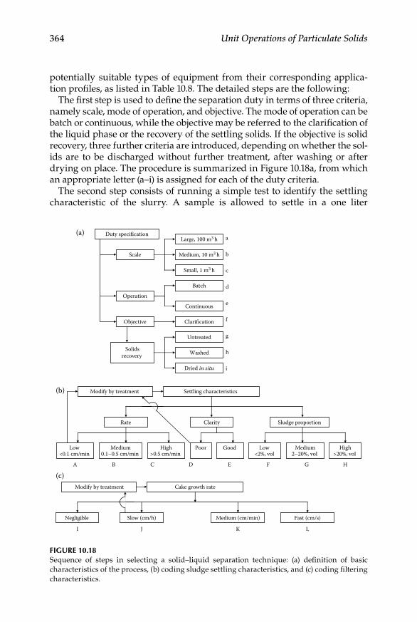
364 Unit Operations of Particulate Solids
potentially suitable types of equipment from their corresponding applica-tion profiles, as listed in Table 10.8. The detailed steps are the following:
The first step is used to define the separation duty in terms of three criteria, namely scale, mode of operation, and objective. The mode of operation can be batch or continuous, while the objective may be referred to the clarification of the liquid phase or the recovery of the settling solids. If the objective is solid recovery, three further criteria are introduced, depending on whether the sol-ids are to be discharged without further treatment, after washing or after drying on place. The procedure is summarized in Figure 10.18a, from which an appropriate letter (a–i) is assigned for each of the duty criteria.
The second step consists of running a simple test to identify the settling characteristic of the slurry. A sample is allowed to settle in a one liter
Cake growth rate
Negligible Slow (cm/h) Medium (cm/min) Fast (cm/s)
Modify by treatment
Modify by treatment
LKJI
(c)
Settling characteristics
Rate Clarity Sludge proportion
Low <0.1 cm/min
Medium0.1–0.5 cm/min
High>0.5 cm/min
Low <2%, vol
Medium2–20%, vol
High>20%, vol
Poor Good
A B C D E F G H
(b)
Duty specification
Scale
Operation
Objective
Large, 100 m3 h
Medium, 10 m3 h
Small, 1 m3 h
Batch
Continuous
Clarification
Untreated
Washed
Dried in situ
Solidsrecovery
a
b
c
d
e
f
g
h
i
(a)
Figure 10.18Sequence of steps in selecting a solid–liquid separation technique: (a) definition of basic characteristics of the process, (b) coding sludge settling characteristics, and (c) coding filtering characteristics.

Solid–Fluid Systems 365
measuring cylinder from about an hour and observations are made for the rate of settling, the clarity of the supernatant layer, and the depth of settling sludge relatively to the total sample depth. The observations are expressed as the corresponding code letters (A–H) giving in the summarized diagram shown in Figure 10.18b. When slurry is found to have poor settling character-istics, pretreatment adding coagulants or flocculants should be considered, and the process should be repeated.
The third step quantifies the filtration characteristic of the slurry from a sec-ond simple test, in which the speed of cake formation is roughly assessed. Using a laboratory Buchner funnel or any other simple suction filter, a small sample of about 200 mL of slurry is filtered and the time is recorded. The observed time and the cake thickness provide a basis to identify the filtration character-istic and assign a code letter (I–L) from those listed in Figure 10.18c. The possi-bility of pretreatment could be contemplated, again, if considered appropriate.
The fourth and final step is used to compare the separation duty profile derived from the three previous steps, with the equipment application profiles listed in Table 10.8 as to identify the most likely equipment for the solid–liquid separation duty.
10.4.3.1 Laboratory Exercise: Settling Tests to Select a Proper Technique
10.4.3.1.1 Introduction
Solid–liquid separations fall into two general categories: those involving clarification, and those dealing with cake formation and separation. Clarification is, generally, an operation to be carried out in equipment other than filters and involving, often, centrifugal forces. Cake formation or recov-ery of solids is a typical operation that may be performed in any type of fil-tering device. The objective of the experiment is to determine the suitability of a filter or a centrifugal device to carry out a separation task at laboratory scale, focusing on the important factor of the concentration of solids.
10.4.3.1.2 Instruments and Materials
The routine laboratory material and glassware to carry out gravimetric test-ing, such as analytical balance, oven, desiccator, and sample containers, would be sufficient for the experiments. There will be need of six to eight one liter measuring cylinders, also. Any type of laboratory centrifuge and a setup to perform filtering consisting of a filter flask, a Buchner funnel, and avail-able vacuum, will complete the supplies needed. Suspensions of a fine pow-der, such as limestone, in water prepared at various concentrations with narrow range, but including both the dilute and concentrated suspension category, that is, 6%, 8%, 10%, 12%, and 14% solids, by volume.
10.4.3.1.3 Procedure
Proceed as described in the previous section, by consulting first •the chart in Figure 10.18a and assign the appropriate letters code.
366 Unit Operations of Particulate Solids
As a first approach, consider clarification for the most dilute sus-pensions and recovery for the concentrated suspensions. The choice of batch or continuous operation may be arbitrary but, again, the most dilute suspensions tend to be treated in continuous equip-ment while the most concentrated tend to be directed to batch equipment.Carry out the first suggested in the previous section testing, that is, •allow samples to settle in a one liter measuring cylinder from about an hour and observe the rate of settling, the clarity of the superna-tant layer, and the depth of settling sludge relatively to the total sam-ple depth. Assign the corresponding code letters using chart in Figure 10.18b.Take on the second suggested test by using a laboratory Buchner •funnel to filter a small sample of about 200 mL of slurry. By using the filtration time and the cake thickness as criteria, identify the filtration characteristic and assign a code letter from those listed in Figure 10.18c.Identify the most likely equipment from the profiles listed in Table •10.8 for the solid–liquid separation duty.From all the choices made, use the results that may considered two •options, one filtering option and another centrifugation-based option, and run tests in a laboratory centrifuge, and in the filtering setup. Compare the quality of the supernatant for both techniques, and choose the one that provides the lowest concentration of sus-pended solids. If the concentration of suspended solids is some-what similar for both techniques, use discriminative criteria, such as the cost of the operation, the time in completing the task, and the labor-demanding feature of each technique. A rough esti-mate of the cost can be worked out by looking at the power of the electric motors of the centrifuge and the vacuum pump used in filtration, in relation to the time they operated to complete the task.
10.4.3.2 Calculations and Report
Present all calculations, if done, for the discriminative criteria of •cost, convenience, and so on, made in choosing one technique over another.Write a complete written report, according to scientific report guide-•lines, either given by an instructor or consulted in the literature. Include graphs, charts, and calculations carried out. Justify the choices made, as scientifically as possible.

Solid–Fluid Systems 367
10.4.4 Sedimentation
10.4.4.1 Introduction
Sedimentation can be defined as a unit operation to perform separation of a suspension into a supernatant clear fluid and dense slurry containing higher concentration of solids. In a more convenient manner, it should be estab-lished that the settling of solids of a suspension in sedimentation is due to gravity force, and industrial sedimentation can be described as the gravita-tional settling of solids suspended in liquids. The uses of sedimentation in industry fall into the categories of solid–liquid separations, solid–solid sepa-rations as in particle classification, and other operations such as mass trans-fer or washing. In solid–liquid separations the solids are removed from the liquid because any, or both, of the phases are more valuable separated or because they have to be separated before disposal. When the primary pur-pose is to produce the solids as highly concentrated slurry the process is called thickening, whereas if the purpose is to clarify the liquid the process is referred to as clarification. Usually, the feed concentration to a thickener is higher that that to a clarifier. Some types of equipment can accomplish both thickening and clarification in a single stage, provided that they are correctly designed and operated.
Sedimentation can be used for size separation, that is, classification of solids, being one of the simplest ways to remove coarse or dense solids from a feed suspension. Successive decantation in a batch system produces closely controlled size fractions of the product. Classification by sedimentation, however, does not produce a sharp separation.
Apart from the above-described applications, sedimentation is also used for other purposes. Relative motion of particles and liquid increases the mass-transfer coefficient. This motion is particularly useful for solvent extraction in immiscible liquid–liquid systems. Another important commer-cial application of sedimentation is in continuous countercurrent washing, where a series of continuous thickeners is used in a countercurrent mode in conjunction with returning of slurry, with the purpose of removing mother liquor or washing soluble substances from the solids.
As settling of solids in sedimentation is caused by the effect of gravity, difference of density between the solids and the suspended liquid is a nec-essary prerequisite. Also, it may be implied that the governing equations describing the process will be those derived in Section 10.1.2, that is, the Stokes law equation (Equation 10.11) and the related equations for sedimen-tation in the different settling regime regions (Equations 10.12 and 10.13). Predicting the settling behavior of particles within a liquid in real sedi-mentation system is, however, rather complicated because there are many factors involved in the process. Among these factors, the distance from the boundaries of the container and from other particles, can be mentioned as critical in affecting settling. Both of these mentioned factors are directly related to the concentrations of solids of the feed stream taken to a given

368 Unit Operations of Particulate Solids
sedimentation unit. It has been suggested that if the relation of the diame-ter of particle to the diameter of the sedimentation vessel is over 1:200 or if the solids concentration by volume is less than 0.2%, any given particle is at sufficient distance from the boundaries of the vessel or from other particles so that its fall is not affected by them. In this case the process is called free settling. Contrastingly, when the motion of the particle is impeded by other particles, which will happen if the particles are near each other even they may not actually be colliding, the process is called hindered settling. The drag coefficient in hindered settling is greater than that in free settling.
10.4.4.2 Free Settling
As previously mentioned, the theory described in Section 10.1.2 including discussion on Equations 10.11 through 10.13 and the need of successive approximations in conjunction with Figure 10.3 to employ them properly, should be applied for calculation of industrial sedimentation within the free-settling regime. There are several cases in which such approximation is possible, for example, in measurement of particle size distribution by sedi-mentation or in particle classification. The approach, however, tends to be theoretical, since complete noninterference of particles settling within a liquid could be only possible for the case of these (the particles) being solitary. Experience has shown that in many real applications of industrial sedimentation correcting factors, mainly for suspension concentration, are needed in order to minimize calculation errors.
10.4.4.3 Hindered Settling
As described above, in concentrated suspensions particles get closer together and interfere with each other. If the particles are not disturbed uniformly, the overall effect is a net increase in settling velocity since the return flow caused by volume displacement predominates in particle-sparse regions. This is the well-known effect of cluster formation which is significant only in nearly monosized dispersions. With most practical widely dispersed sus-pensions clusters do not survive long enough to affect the settling behavior and, as the return flow is more uniformly distributed, the settling rate steadily declines with increasing concentration. This phenomenon of hin-dered settling and can be theoretically approached in three different man-ners: as a Stokes’ law correction by introduction of a multiplying factor, by adopting effective fluid properties for the suspension different from these of the pure fluid, and by determination of bed expansion with a modified ver-sion of the well-known Carman–Kozeny equation. All the approaches can be shown to yield essentially identical results.
Svarovsky (1984) reviewed some important correlations accounting for the hindered settling effect and demonstrated that their differences are minimal.
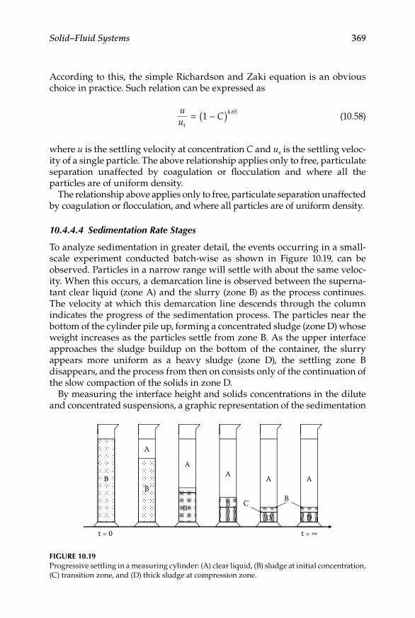
Solid–Fluid Systems 369
According to this, the simple Richardson and Zaki equation is an obvious choice in practice. Such relation can be expressed as
uu
Ct
= −( )1 4 65.
(10.58)
where u is the settling velocity at concentration C and us is the settling veloc-ity of a single particle. The above relationship applies only to free, particulate separation unaffected by coagulation or flocculation and where all the particles are of uniform density.
The relationship above applies only to free, particulate separation unaffected by coagulation or flocculation, and where all particles are of uniform density.
10.4.4.4 Sedimentation Rate Stages
To analyze sedimentation in greater detail, the events occurring in a small-scale experiment conducted batch-wise as shown in Figure 10.19, can be observed. Particles in a narrow range will settle with about the same veloc-ity. When this occurs, a demarcation line is observed between the superna-tant clear liquid (zone A) and the slurry (zone B) as the process continues. The velocity at which this demarcation line descends through the column indicates the progress of the sedimentation process. The particles near the bottom of the cylinder pile up, forming a concentrated sludge (zone D) whose weight increases as the particles settle from zone B. As the upper interface approaches the sludge buildup on the bottom of the container, the slurry appears more uniform as a heavy sludge (zone D), the settling zone B disappears, and the process from then on consists only of the continuation of the slow compaction of the solids in zone D.
By measuring the interface height and solids concentrations in the dilute and concentrated suspensions, a graphic representation of the sedimentation
t = 0
BB
A
B
AA
B
A
D
A
D
C
t = ∞
B
Figure 10.19Progressive settling in a measuring cylinder: (A) clear liquid, (B) sludge at initial concentration, (C) transition zone, and (D) thick sludge at compression zone.

370 Unit Operations of Particulate Solids
process can be prepared as shown in Figure 10.20. The plot shows the differ-ence in interface height plotted against time, which is proportional to the rate of settling as well as to concentration.
As follows from an earlier discussion on spheres falling through a fluid medium, sedimentation is faster in liquids having low viscosities. Thus, sedimentation rates are higher at elevated temperatures. As also mentioned, an increase in the process rate may be achieved by increasing particle sizes through the use of coagulation or agglomeration, or by adding an electrolyte in the case of colloidal suspensions.
10.4.4.5 Operating Principles: Design and Selection Factors
Sedimentation equipment can be divided into batch-operated settling tanks and continuously operated thickeners or clarifiers. The operation of the former is very simple and their use has recently diminished. They are still used, however, when small quantities of liquids are to be treated. Most sedi-mentation processes operate in continuous units.
The conventional thickeners are constructed of steel in sizes less than 25 m diameter, or concrete in larger tanks that usually range up to 100 m diameter. The floor is often sloped toward the underflow discharge in the center. The tanks usually include a raking mechanism, which turns slowly around the center column in order to promote solids consolidation in the compression zone while aiding the underflow discharge. The rake arms are driven by fixed connections or dragged by cables or chains suspended from a drive arm that is rigidly connected to the drive mechanism. The rake arms are also con-nected to the bottom of the central column by a special arm hinge that allows both horizontal and vertical movements. This arrangement lifts the rakes automatically if the torque becomes excessive. The drive arm can be attached below the suspension level or, if scaling is a problem, above the basin. Figure 10.21 shows a diagram of a conventional circular section thickener.
Time
Clea
r liq
uid
inte
rface
hei
ght
Constant rate
Ultimate height
C
Figure 10.20Sedimentation rate graph.
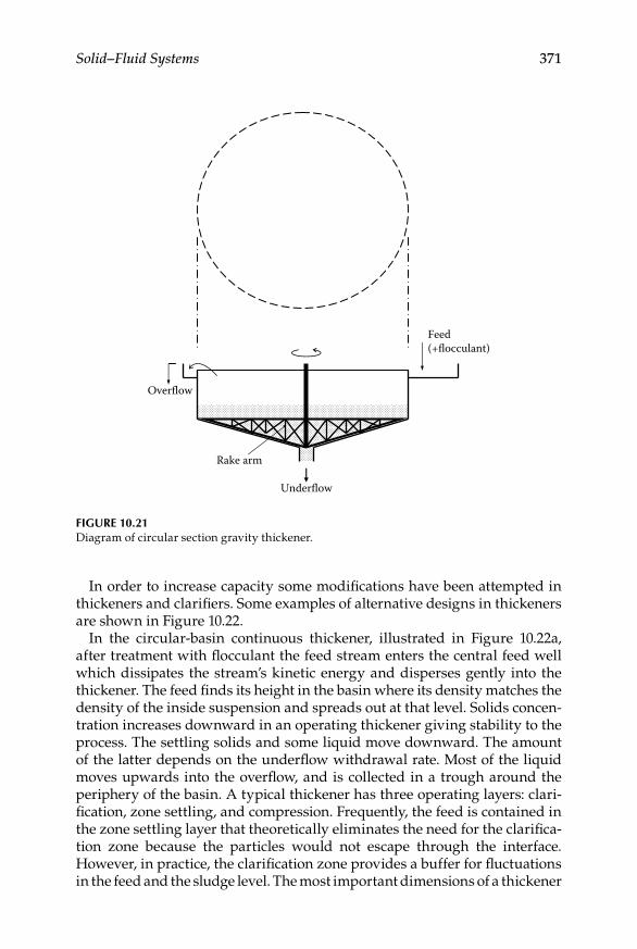
Solid–Fluid Systems 371
In order to increase capacity some modifications have been attempted in thickeners and clarifiers. Some examples of alternative designs in thickeners are shown in Figure 10.22.
In the circular-basin continuous thickener, illustrated in Figure 10.22a, after treatment with flocculant the feed stream enters the central feed well which dissipates the stream’s kinetic energy and disperses gently into the thickener. The feed finds its height in the basin where its density matches the density of the inside suspension and spreads out at that level. Solids concen-tration increases downward in an operating thickener giving stability to the process. The settling solids and some liquid move downward. The amount of the latter depends on the underflow withdrawal rate. Most of the liquid moves upwards into the overflow, and is collected in a trough around the periphery of the basin. A typical thickener has three operating layers: clari-fication, zone settling, and compression. Frequently, the feed is contained in the zone settling layer that theoretically eliminates the need for the clarifica-tion zone because the particles would not escape through the interface. However, in practice, the clarification zone provides a buffer for fluctuations in the feed and the sludge level. The most important dimensions of a thickener
Feed(+flocculant)
Underflow
Overflow
Rake arm
Figure 10.21Diagram of circular section gravity thickener.
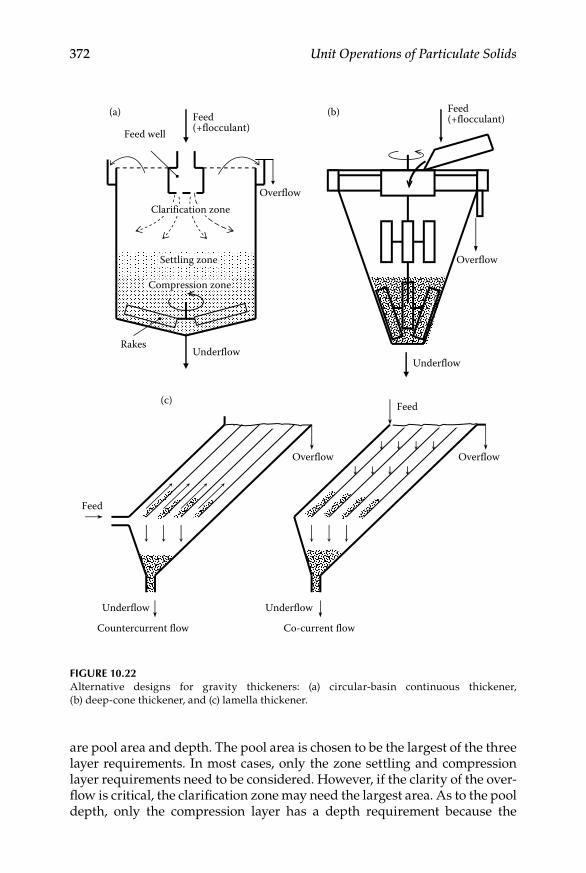
372 Unit Operations of Particulate Solids
are pool area and depth. The pool area is chosen to be the largest of the three layer requirements. In most cases, only the zone settling and compression layer requirements need to be considered. However, if the clarity of the over-flow is critical, the clarification zone may need the largest area. As to the pool depth, only the compression layer has a depth requirement because the
Feed
Underflow
Overflow
Underflow
Overflow
Feed
Countercurrent flow Co-current flow
Feed(+flocculant)Feed well
(a) (b)
(c)
Settling zone
Compression zone
Underflow
Overflow
Rakes
Underflow
Overflow
Feed(+flocculant)
Clarification zone
Figure 10.22Alternative designs for gravity thickeners: (a) circular-basin continuous thickener, (b) deep-cone thickener, and (c) lamella thickener.

Solid–Fluid Systems 373
concentration of the solids in the underflow is largely determined by the time detention and, sometimes, by the static pressure. Thickness of the other two layers is governed only by practical considerations. The deep-cone thick-ener (Figure 10.22b), based on the deep-cone vessel used for the processing of coal and metallurgical ores, is equipped with a slow-turning stirring mecha-nism, which enhances flocculation in the upper part and acts as a rake in the lower section. The unit is used for densification of froth-flotation tailings at overflow rates from 6.5–10 m/h to a final discharge containing 25–35% moisture by weight. Other commercial deep-cone thickeners are of particu-lar advantage where the final underflow density is increased by the large static head above the discharge point, for example, with flocculated clays. Another development is the Swedish Lamella thickener shown in Figure 10.22c. It consists of a number of inclined plates stacked closely together. In the countercurrent design, the flocculated feed enters the stack from a side feed box. The flow moves upward between the plates while the solids settle onto the plate surfaces and slide down into the sludge hopper underneath where they are further consolidating by vibration or raking. In theory, the effective settling area is the sum of the horizontal projected areas of all plates. In practice, however, only about 50% of the area is utilized. When treating sticky sludges, the whole lamella pack can be vibrated intermittently con-tinuously to assist the sliding motion of the solids down the plates. In some instances, the plates are corrugated instead of flat, or they are replaced by tube bundles becoming what is known as a tube settler.
Thickeners are designed by the traditional Coe and Clevenger, or Talmage and Fitch procedures (Fitch, 1975), which use batch-settling data to evaluate the whole concentration range right up to the underflow concentration, even though a batch-settling test cannot possibly simulate the continuous- thickener process. The design procedures are based on plotting total flux versus concentration, as shown in Figure 10.23a. The concentration of the solids continuously increases from the feed value Cf, to the underflow concentration Cu. The total flux plot goes through a minimum (the critical flux Gc) on which the design area A is based, according to a mass balance, on the following relation:
A
QCG
= f
c (10.59)
where Q is the mass flow rate of particles by volume.The total flux plot depends not only on the settling characteristics of the
solids, but also on the selected underflow concentration because total flux includes the transport flux, or dead flux, contributed by movement of particles downward as underflow is withdrawn. The plot can be made independent of Cu by subtracting the transport flux contribution from Gc, and plotting the resultant settling flux Gs, as done in Figure 10.23b. A line drawn tangentially
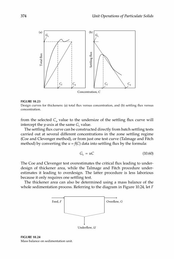
374 Unit Operations of Particulate Solids
from the selected Cu value to the undersize of the settling flux curve will intercept the y-axis at the same Gc value.
The settling flux curve can be constructed directly from batch settling tests carried out at several different concentrations in the zone settling regime (Coe and Clevenger method), or from just one test curve (Talmage and Fitch method) by converting the u = f(C) data into settling flux by the formula:
G uCs = (10.60)
The Coe and Clevenger test overestimates the critical flux leading to under-design of thickener area, while the Talmage and Fitch procedure under-estimates it leading to overdesign. The latter procedure is less laborious because it only requires one settling test.
The thickener area can also be determined using a mass balance of the whole sedimentation process. Referring to the diagram in Figure 10.24, let F
Gc
Tota
l flu
x Gc
(a) (b)
Cf Cu Cf Cu
Settl
ing
flux
Concentration, C
Figure 10.23Design curves for thickeners: (a) total flux versus concentration, and (b) settling flux versus concentration.
Feed, F
Underflow, U
Overflow, O
Figure 10.24Mass balance on sedimentation unit.

Solid–Fluid Systems 375
be the mass flow rate of solids in the feed, U the mass flow rate of solids in the underflow, O the mass flow rate of solids in the overflow, XF the fraction of solids in the feed, XU the fraction of solids in the underflow, 1 – XF the frac-tion of liquid in the feed, and 1 – XU the fraction of liquid in the underflow.
The mass balances of liquid and solids in the process can be represented by
F X O X( ) ( )1 1− = + −F U (10.61)
F X U X( ) ( )F U= (10.62)
It can be demonstrated that
O
F X XX
= −( )U F
U (10.63)
For the limiting conditions of producing a clear overflow, the terminal set-tling velocity of the particles ut should be equal to the ascending velocity of the liquid u↑, so that
u u
OAt
Flowrate (volumetric)Area= = =↑ ρ
(10.64)
Substituting Equation 10.64 into Equation 10.63, transposing for A and call-ing it minimum area Amin:
A
F X XX umin = −( )U F
U tρ (10.65)
With regard to clarifiers, the conventional one-pass unit employs horizontal flow in circular or rectangular vessels. Figure 10.25 shows a schematic dia-gram of a rectangular basin with feed at one end and overflow at the other. The feed can be preflocculated in an orthokinetic flocculator that may form part of the unit. Settled solids are pushed to a discharge trench by paddles or blades on a chain mechanism or suspended from a traveling bridge. Circular basin clarifiers are most commonly fed through a centrally located feed well; the overflow is led into a trough around the periphery of the basin. The bot-tom gently slopes to the center and the settled solids are pushed down the slope by a number of motor-driven scraper blades that revolve slowly around a vertical center shaft. Like thickeners, circular clarifiers can be stacked in multitray arrangements to save space.
Clarifier performance depends on area, which is determined by the flocculation nature of the feed suspension. When the overflow clarity is

376 Unit Operations of Particulate Solids
independent of overflow rate and depends only on detention time, the required time is determined by simple laboratory testing of residual solid concentrations in the supernatant versus detention time under the condi-tions of mild shear. This determination is sometimes called the second-order test procedure because the flocculation process follows a second-order reaction rate. In most cases, clarifying performance depends on detention time and overflow rate. Tests are conducted in a vertical tube that is as long as the expected depth of the clarifier, under the ideal assumption that a verti-cal element of a suspension, which has been clarified, maintains its shape as it moves across the tank.
If the suspension is nonflocculant, or if flocculation takes place prior to settling, the overflow clarity is independent of detention time and depends only on the overflow rate Q according to the relation:
Q A umax ( )= t (10.66)
in this case the settling velocity ut is expressed by
u
Htt =
(10.67)
where ut is the maximum particle settling velocity that yields a satisfactory clarity in a simple laboratory sedimentation test, H is the height of the laboratory container, and t is the time in which the supernatant liquid becomes clear.
Feed
Overflow
Underflow
Sludge dragging paddles
Figure 10.25Diagram of rectangular-basin clarifier.

Solid–Fluid Systems 377
For nonflocculant suspensions, gravity clarifiers are sometimes used as for solids classification. The theoretical grade efficiency curve G(x) of the clari-fier can be predicted, assuming laminar flow and no end effects, by
G x
A uQ
( )( )= t
(10.68)
where ut is a function of particle size and can be found from Equation 10.11 if Stokes law applies.
example 10.5
A 25% solids concentrated suspension contains particles of approximate spheri-cal shape of an insoluble food powder. The mean size of the particles is 50 μm and their density is 2002 kg/m3. Calculate the settling velocity of such particles in water at room temperature.
SoluTion
Due to the size and density of particles, a reasonably assumption would be settling within the Stokes law region. Properties of water can be consulted in Appendix 2. Using, thus, Equation 10.11, the terminal settling velocity is
ut
2 3 2m kg/m m/skg/m s
136 m= × =−( ) ( ) ( . )
( . ).
5 10 1002 9 8118 0 001
0 005 2
//s
Verifying the applicability of the chosen sedimentation region, by calculating the particle Reynolds number:
Re
( ) ( ) ( . ).
.p
3m kg/m m/skg/m s
= × =−5 10 1000 0 00136
0 0010 06
5
The approximation was correct and the settling time is valid. Finally, due to the high concentration of solids, correction due to this factor is in order. Transposing for the corrected settling velocity from Equation 10.58 and substituting values, the real settling velocity is
u u C= − = − =t 357 m/s( ) ( . )( . ) .. .1 0 00136 1 0 25 0 0004 65 4 65
10.4.4.6 Laboratory Exercise: Acceleration of Settling Rates by Coagulants
10.4.4.6.1 Introduction
Coagulation and flocculation are used to increase the effective particle size, thereby improving sedimentation settling rates. Coagulation produces

378 Unit Operations of Particulate Solids
particles up to 1 mm in diameter, while flocculation renders flocs up to 1 cm in size. The objective of the exercise is to verify the advantage of adding a coagulant to a concentrated suspension, by comparing settling rates with and without the coagulant addition.
10.4.4.6.2 Instruments and Materials
Five or six 1-L measuring cylinders are required. A concentrated suspension of a fine powder, for example, limestone or starch in water, is also necessary. Any known coagulant agent, such as Al2(SO4)3 or Fe2(SO4)3.
10.4.4.6.3 Procedure
Shake the suspension well and allow it to settle in the one-liter mea-•suring cylinder.Record the clear liquid interfase height related to time, until it stabi-•lizes. Make replicates to give statistical meaning to the exercise.Repeat the procedure adding Al• 2(SO4)3 or Fe2(SO4)3 as the coagulant agent.
10.4.4.6.4 Calculations and Report
Construct graphs of rate of sedimentation (Figure 10.20) for both •sedimentation processes.Locate the point of inflexion (critical point) for each graph.•If critical points appear distant in both graphs, run a statistical test •to determine whether they are significantly different.Write a complete written report, according to scientific report guide-•lines, either given by instructor or consulted in the literature. Include graphs, charts, and calculations carried out.
10.4.5 Centrifugation
10.4.5.1 Introduction: Centrifugal Techniques
As previously discussed, apart from gravity, centrifugal force can also be used to separate solids in suspension. Centrifugal sedimentation is a tech-nique in which the suspension is subjected to a centrifugal field, to cause the solid particles to move radially apart from the center of rotation and lead to separation. A significant density difference between solid and liquid is a necessary prerequisite in sedimentation of any kind. Centrifugal sedimenta-tion can be carried out in two types of equipment: rotated wall devices and fixed wall devices. Rotating wall devices are also known as centrifuges. The most popular fixed wall device is the hydrocyclone. The term “centrifuga-tion” has been traditionally used to imply the operation of centrifugal sedimentation in rotating wall devices.

Solid–Fluid Systems 379
10.4.5.2 Applications of Centrifugation
Centrifugation presents varied and diverse applications in different process-ing industries. Many types of separations can be carried out through cen-trifugation, as long as a significant density difference between solid and liquid exists. The most common applications of centrifugation in processing industries are: (a) liquid–liquid separations, (b) centrifugal clarification, (c) sludge separation, and (d) centrifugal filtration.
Within the context of particle technology, the most relevant application of centrifugation is centrifugal clarification since it follows theoretical princi-ples of dynamics of particles submerged in fluids as discussed in this book. Those principles are used to describe centrifugal clarification as a unit operation.
10.4.5.3 Centrifugal Clarification
Centrifugal clarification is the term used to describe the removal of small quantities of insoluble solids from a fluid by centrifugal means. If a dilute suspension containing solids with a greater density than the liquid is fed to a rotating cylindrical bowl, the solids will move toward the bowl wall. If an outlet is provided for the liquid near the center of rotation, then those parti-cles of solid which reach the bowl wall will remain in the bowl. Those par-ticles that do not reach the bowl wall will be carried out in the liquid. The fraction remaining in the bowl and the fraction passing out in the liquid will be controlled by the feed rate, that is, the dwell time, in the bowl. If a solid particle of diameter x moves radially in a liquid within a rotating bowl, at its terminal velocity under laminar flow conditions the radial velocity of the particle will be represented by Equation 10.31. The time required for a particle to travel an elemental radial distance, dR, is
d
d dr
2s
tR
v xR
R= =
−⋅18
2
µω ρ ρ( )
(10.69)
Assuming that half of all those particles present in the feed with a particular diameter xc are removed during their transit through the bowl, those parti-cles with diameters greater than xc will be mostly removed from the liquid, whereas those particles with diameters smaller than xc will be likely to remain in the liquid. In this context xc as here defined is known as the “cut-point” or “critical” diameter.
If clarification takes place in a simple cylindrical centrifuge with cross sec-tion as shown in Figure 10.26, all particles of diameter xc contained in the outer half of the cross-sectional area of the ring of liquid will reach the bowl wall and will be removed from the liquid. The maximum distance that a particle in this zone has to travel to reach the bowl wall is R R R2 1
222 1 22− +[( )/ ] ,/

380 Unit Operations of Particulate Solids
as indicated in Figure 10.26. The time required for a particle of diameter xc to travel this distance is
tx
RR
R R
R
= − ∫18µω ρ ρ2
s c2
+ )/2]
d
12
22 1/2
2
( )[(
(10.70)
Integrating Equation 10.70 and substituting limits the following relation is obtained:
t
R R R
x=
( )−
182
µ
ω ρ ρ
ln
( )2 1
222 1/2
2s c
( )/2+
(10.71)
The minimum residence time for a particle in the bowl is V/Q, where V is the volume of liquid held in the bowl at any time and Q is the volumetric flow rate of liquid through the bowl. Thus, for a particle of diameter xc to be separated out
VQ
R R R
x=
( )−
18µ
ω ρ ρ
ln
( )2 1
222 1/2
2s c
2
( )/2+
(10.72)
R12 + R2
2
2
R1
R2
Figure 10.26Schematic diagram of radial separation zones in the cross section of a centrifugal clarifier.

Solid–Fluid Systems 381
Equation 10.72 may be written in the form:
Qg x V
g R R R=
−
⋅ ( )
2 18 2
( )
ln
ρ ρµ
ωs c2 2
2 12
22 1/2
( )/2+
(10.73)
The first term of Equation 10.73 includes the previously discussed expression for Stokes’ law, that is, Equation 10.11. Thus, another way of expressing Equation 10.73 is as follows:
Q u= 2 gΣ (10.74)
where ug is the terminal settling velocity of a particle of diameter xc in a gravitational field and Σ is a characteristic parameter of any given centrifuge; equivalent to the area of a gravity settling tank with similar settling characteristics to the centrifuge, that is, one which will remove half of all particles of diameter xc. Different values of Σ are given in the literature (McCabe et al., 2005). For a simple cylindrical bowl centrifuge:
Σ ≈ +πω2b R R
g( )3
222
12
(10.75)
where b is the height of the bowl. Also, for a disc-bowl centrifuge:
Σ Ω=
− −2 13
2πω ( )( )tan
S R Rg
x y3 3
(10.76)
where S is the number of discs in stack, Rx and Ry are the outer and inner radii of stack, respectively, and Ω is the conical half-angle of discs (Trowbridge, 1962).
10.4.5.4 Centrifugal Filtration
The term describes the separation of solids from a liquid by filtration for the case of the filtrate flow being induced by centrifugal means. The general principle of the filtering centrifugal is shown in Figure 10.27. As can be observed, a suspension is fed into a rotating bowl with a perforated wall, which is lined with a suitable filter medium. The solids are forced onto the bowl wall giving rise to a filter cake through which the filtrate passes, under the influence of centrifugal force. The filtrate makes its pass through the filter medium and perforated wall also and, finally, into an outer casing and out a discharge port. Wash liquid may be sprayed through the solids to remove
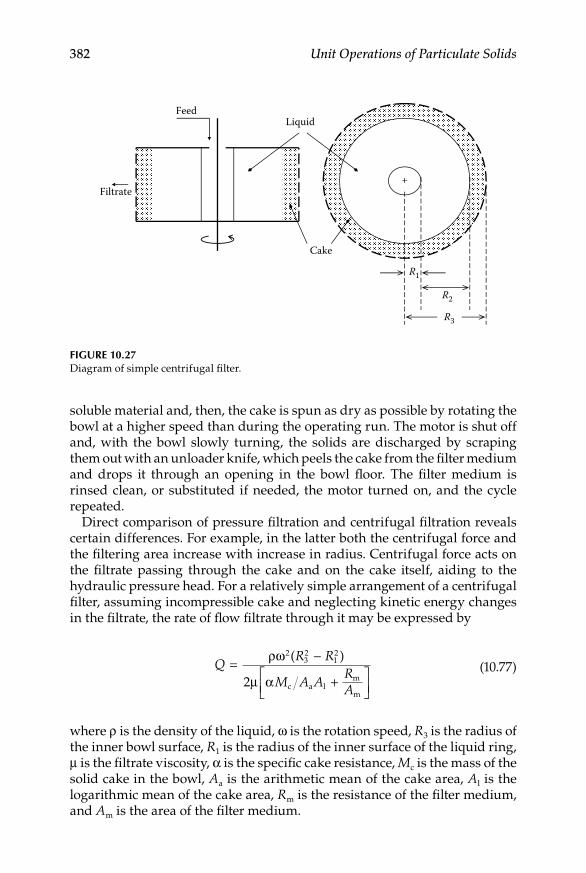
382 Unit Operations of Particulate Solids
soluble material and, then, the cake is spun as dry as possible by rotating the bowl at a higher speed than during the operating run. The motor is shut off and, with the bowl slowly turning, the solids are discharged by scraping them out with an unloader knife, which peels the cake from the filter medium and drops it through an opening in the bowl floor. The filter medium is rinsed clean, or substituted if needed, the motor turned on, and the cycle repeated.
Direct comparison of pressure filtration and centrifugal filtration reveals certain differences. For example, in the latter both the centrifugal force and the filtering area increase with increase in radius. Centrifugal force acts on the filtrate passing through the cake and on the cake itself, aiding to the hydraulic pressure head. For a relatively simple arrangement of a centrifugal filter, assuming incompressible cake and neglecting kinetic energy changes in the filtrate, the rate of flow filtrate through it may be expressed by
QR R
M A ARA
= −
+
ρω
µ α
2
2
( )32
12
c a lm
m
(10.77)
where ρ is the density of the liquid, ω is the rotation speed, R3 is the radius of the inner bowl surface, R1 is the radius of the inner surface of the liquid ring, μ is the filtrate viscosity, α is the specific cake resistance, Mc is the mass of the solid cake in the bowl, Aa is the arithmetic mean of the cake area, Al is the logarithmic mean of the cake area, Rm is the resistance of the filter medium, and Am is the area of the filter medium.
R1
R2
R3
Feed Liquid
Filtrate
Cake
+
Figure 10.27Diagram of simple centrifugal filter.

Solid–Fluid Systems 383
Equation 10.77 is applicable only for cakes of uniform thickness. In many practical cases cakes are thicker near the bottom than at the top of bowl. Such systems will give a filtration rate 5–20% greater than a cake of constant thickness of similar volume and permeability (Green and Perry, 2008).
example 10.6
A viscous suspension contains particles of a solid of 1461 kg/m3 density, and is to be clarified by centrifugation. The liquid has a density of 801 kg/m3 and a viscos-ity of 100 cp. A clarifying centrifuge with bowl 44.5 diameter and 197 mm height is used. During operation an annular air core of 14.23 mm diameter is formed. Calculate the cut point for a capacity of 169.92 L/h, when the centrifuge runs at 23,000 rpm speed.
SoluTion
To facilitate calculation, it is recommended to transform all the data to SI units. The viscosity is 0.1 kg/m s in SI units. Pertaining geometrical features, according to diagram in Figure 10.26: R2 = 0.0225 m, R1 = 0.00761 m, and b = 0.197 m. Finally, the capacity is 4.7245 × 10⁻⁵ m3/s, and the rotation speed is 2410 rad/s (2410 L/s), from the relation ω = (2πN)/60, where N is rotational speed in rpm. With all the data in SI units, from Equation 10.75, the value of Σ is
Σ =
+ 3 14 2410 0 197 3 0 02225 0 00716
2 9
2 2 2. ( ) ( )( . ) ( . ) ( . )
(
1/ m m2 2s
.. ).
81281 5
m/sm2
2=
Finally, transposing for the cut point xc from Equation 10.74 and solving:
xc
3
2 3
kg/m s m /sm/s kg/m
= ×−
=−18 0 1 4 725 10
2 9 81 1461 801
5( . ) ( . )( . ) ( )
44 83 10 6. × − m
Thus, the cut point is 4.8 μm, approximately.
10.4.5.5 Fixed Wall Devices: Hydrocyclones
The use of hydrocyclones is another possibility to separate suspended solids from a liquid taking advantage of the centrifugal force. The operating prin-ciple of a hydrocyclone is similar to that of a cyclone (Figure 10.7), differing only in the geometrical proportions due to the difference in magnitudes of properties between gases and liquids. Since liquids possess densities and viscosities proportionally much higher than gases, in hydrocyclones Δρ is much narrower than in cyclones. Also, for the same reason of properties of phases, the viscous forces opposing settling of particles within a liquid are much greater than those within a gas. Hydrocyclone units have, therefore, proportionally much smaller diameters than cyclones. In such a manner the liquid flow, proportionally more dense and viscous than a gas flow, would
384 Unit Operations of Particulate Solids
give origin to a vortex within the hydrocyclone with centrifugal force sufficient to separate solid particles.
Similar to cyclones and centrifuges, hydrocyclones may be evaluated in terms of separation efficiency by means of the cut size or cut point (xc or x50). The criteria to define and interpret efficiency, along with definitions and use-fulness of the cut point concept, have been discussed in Section 10.2. Numerous analytical expressions to calculate the cut point for hydrocy-clones have been suggested (Ortega-Rivas, 1989), but the most convenient way of evaluating it is, arguably, using the grade efficiency curve also dis-cussed in Section 10.2. Due to the effect of concentration of suspensions, than will be normally much higher for hydrocyclones than for cyclones, the grade efficiency curve should be derived taking into account the dead flux effect as to obtain reduced grade efficiency curves (Section 10.2.4) like the example given in Figure 10.5 from calculations using Equation 10.29.
Since hydrocyclones do not have any rotating parts and the vortex action to produce centrifugal force is obtained by pumping the feed suspension tangentially into the cono-cylindrical body, the literature is full of studies of the effects of the relative geometric proportions on pressure drop or capacity and separation efficiency. Using this information hydrocyclone geometry could be selected to obtain an optimum performance in terms of cut size. In this sense, possibly the best opportunity to predict hydrocyclone perfor-mance is the use of a dimensionless scale-up model well described elsewhere (Ortega-Rivas and Svarovsky, 1993). Three dimensionless groups can be used to describe hydrocyclone operation and performance: the Euler number Eu, the Reynolds number Re, and the Stokes number Stk50. For best application of the relationships among dimensionless groups, certain proportions must be unchanged. Such proportions are generally reported as a function of the diameter of the hydrocyclone. There are several different standard hydro-cyclone designs in which proportions remain the same regardless of size. One of the most efficient designs for separation is called the Rietema (1961) cyclone, whose proportions are illustrated in Figure 10.28.
The Euler number, which is a pressure loss factor, is defined as the limit of the maximum characteristic velocity v obtained by a certain pressure drop ΔP across the hydrocyclone. It can be expressed as
Eu = 2
2
∆Pvρ
(10.78)
where ρ is the liquid density and v is the superficial velocity in the hydrocy-clone body.
The Reynolds number defines flow features of the system and, in the case of hydrocyclones, the characteristic dimension may be taken as the cyclone body diameter Dc:
Re = D vc ρ
µ (10.79)

Solid–Fluid Systems 385
where ρ is the liquid density and μ is the average viscosity.The Stokes number may be derived from basic fluid mechanics theory and
is defined as follows:
Stk50
s
c= −x v
D502
18( )ρ ρ
µ (10.80)
where x50 is the cut size, ρs is the solids density, and Dc is the hydrocyclone diameter.
It can be demonstrated (Svarovsky, 1984) that, similar to the case of cyclones, the most appropriate characteristic velocity to describe hydro-cyclone operation is the superficial velocity in the hydrocyclone body des cribed by Equation 10.38.
Owing to the effect of the suspension concentration that has an influence in the dead flux effect, sufficiently discussed in previous sections, the concentration as a fraction C and the underflow-to-throughput ratio Rf are
0.34 Dc
20°
0.28 Dc 0.4 Dc
Dc
5 Dc
0.2 Dc
Figure 10.28Rietema’s optimum standard geometry hydrocyclone.

386 Unit Operations of Particulate Solids
included in the dimensionless scale-up of hydrocyclone operation as addi-tional dimensionless groups. The underflow-to-throughput is defined as
R
UQf =
(10.81)
where U is the underflow rate and Q is the feed rate.The dimensional analysis gives basic relationships between the above-
mentioned dimensionless groups, which are useful to describe hydrocyclone operation and are the basis for scale-up calculations aimed at adapting results from laboratory experimentation to an industrial scale for a number of processes in diverse industries. For example, for feed suspensions up to 10% by volume Medronho and Svarovsky (1984) proposed the following relations, for hydrocyclones following Rietema’s optimum proportions and treating inert solids suspensions:
Stk Eu e50 ( ) . ln
.
( . )rR
C=
0 047
10 74
8 96
f (10.82)
Eu ei
c=
−−
71 0 1161 3
2 12(Re) ..
( . )DD
C
(10.83)
R
DDf
u
cEu=
−−1218
4 750 30
..( )
(10.84)
where Di, Dc, and Du are the inlet, body, and underflow diameters of the hydrocyclone, respectively. The term (r) accompanying Stk50 is included to indicate that the “reduced” grade efficiency was used to determine the “reduced” cut size x50, in order to account for the dead flux effect.
For concentrations higher than 10% by volume, many practical slurries show non-Newtonian behavior and it can be shown (Ortega-Rivas and Svarovsky, 1993) that Reynolds and Stokes numbers can be reexpressed to consider such behavior. The correlations derived under this mentioned consideration are the following:
Stk Eu e50
*
f( ) . ln
.
( . )r R=
0 006
12 37
6 84C
(10.85)
Eu e= − −1686 0 035 3 39(Re )* . ( . )C (10.86)
R
DD
Cf
u
ce=
−32 81 53
0 34 3 70. (Re ).
* . ( . )
(10.87)

Solid–Fluid Systems 387
where Stk50* and Re* are the “generalized” Stokes and Reynolds numbers,
meaning that they include the parameters of characterization of non- Newtonian suspensions, that is, the fluid consistency index K′ and the flow behavior index n, instead of the medium viscosity (Ortega-Rivas and Svarovsky, 1993). The term generalized is used to imply that, for Newtonian suspensions, Stokes and Reynolds numbers above would reduce to the common forms normally found in the literature. The term (r) accompanies, again, (Stk )*
50 for the same reasons already given.
example 10.7
Determine the cut size obtained when treating 1 L/s of a suspension of inert solids in water, with concentration of 5% by volume, in a Rietema’s standard geom-etry hydrocyclone 1 in. in diameter and 5 mm in underflow opening. The solids density is 2150 kg/m3 and the available pressure drop of operation is 2 × 10⁵ Pa.
SoluTion
The low-suspension concentration will allow use of the properties of the suspend-ing medium in calculations. Reasonable values for density and viscosity of water at approximate room temperature are 1000 kg/m3 and 0.001 kg/m s, respec-tively. The feed rate F(Q) is 0.001 m3/s and the pressure drop 2 × 10⁵kg/s2 m, both expressed in fundamental SI units. The characteristic velocity within the hydro-cyclone can be calculated from Equation 10.38:
v = =4 0 001
3 1416 0 02541 972
( . ). ( . )
.m /s
mm/s
3
2
Using the above-calculated velocity, Eu can be calculated from Equation 10.78, that is,
Eu
kg/s mkg/m m/s
2
3= × =2 2 101000 1 97
102 75( )
( ) ( . ).
once having the value of Eu, since the suspension concentration is low, Equation 10.84 can be used to calculate Rf as
Rf
mm
=
=−12180 005
0 0254102 7 0 1346
4 75
0 3..
( . ) ..
.
the calculated values of Eu and Rf, can then be substituted into Equation 10.82 to transpose for the Stokes number and calculating it, that is,
Stk50( )
ln( / . ) exp . ( . )
..
.
r = [ ] =
1 0 1346 8 96 0 05
102 70 0019
0 74

388 Unit Operations of Particulate Solids
Finally, from the original definition of the Stokes number given in Equation 10.80, and transposing for x50:
x50
0 0019 18 0 001 0 02542150 1000 1 97
=−
( . )( )( . ) ( . )( ) ( .
kg/ms mkg/m3 ))
.m/s
m
= ×1 55 105
The cut point is: x50 ~ 15 μm.
10.4.5.6 Centrifugation Equipment
Generally, the main types of equipment to carry out centrifugation duties in industry coincide in a way with the classification of centrifugation modes described in this book. Regardless of the criteria used to categorize centrifu-gation equipment, it is reasonably to classify centrifuges into: centrifugal clarifiers (tubular and disc bowl) used not only for clarification but for liquid–liquid separation, sludge or decanting centrifuges, and filtering cen-trifuges. Regarding hydrocyclones, apart from Rietema’s geometry already defined there are some other designs available like the Bradley’s hydrocy-clone (Bradley, 1965), but geometric proportions really do not vary much. The alternatives in terms of hydrocyclone manufacturing relate to arrangements in series to provide the best possible efficiency at the highest attainable capacity.
Tubular and disc-bowl centrifuges are designs normally used for clarifi-cation. Figure 10.29 illustrates a tubular-bowl centrifuge consisting on a long and narrow cylindrical bowl rotating at high speed in an outer sta-tionary casing. The feed is introduced through a stationary pipe at the bot-tom of the bowl, and quickly accelerated to the bowl speed by means of vanes or baffles. The two liquids are removed from the annular layers formed through a circular weir system, as shown in Figure 10.29. The con-trol over the neutral zone radius is exercised by fitting rings with different internal diameters to the dense phase outlet. The solids capacity of a tubu-lar bowl machine is seldom more than 2–5 kg and for economical operation the solids content of the feed should normally not exceed about 1% by weight. Disc-bowl centrifuges (Figure 10.30) comprise a relatively shallow, wide cylindrical bowl, rotating at moderate speed in a stationary casing. The bowl contains closely spaced metal cones, or discs, which rotate with the bowl and are placed one above the other with fixed clearance between them. The discs have one or more sets of matching holes in order to form channels through which the feed material flows. Under the influence of centrifugal force the dense phase, traveling toward the bowl wall, streams down the undersides of the discs while the light phase, displaced toward the center, flows over the upper faces of the discs. The liquids are thus divided into thin layers and the distance any drop of the liquid must travel to get caught up the appropriate outgoing stream is very small. The separated

Solid–Fluid Systems 389
liquids are removed by a weir system and, like in the case of tubular centrifuges, different gravity discs on the dense phase outlet need to be used to control the neutral zone position. Disc-bowl centrifuges have solids capacities in the range of 2–20 kg and are usually only suited to clarifying feeds with less than a few percent by weight of solids. Both, tubular and disc-bowl centrifuges, are useful for removing small traces of solids to produce clear liquids, especially if the solids are gelatinous in nature and unsuited to filtration.
Feed
Dense phase
Lightphase
Light liquid Heavy liquid
Gravity disc
Figure 10.29Diagram of tubular-bowl centrifuge.

390 Unit Operations of Particulate Solids
The nozzle-discharge (self-cleaning) and the valve-discharge (self- opening) centrifuges are sophisticated pieces of equipment designed to give continuity to the solid–liquid centrifugation process. A diagram of a nozzle-discharge centrifuge is given in Figure 10.31. As can be seen this centrifuges have a biconical bowl with a number of holes (approximately 0.3 cm in diam-eter) spaced around it at its largest diameter. The solids removed from the liquid are continuously discharged, in the form of thick slurry, into an outer casing. Feeds containing up to 25% solids can be handled in this type of clarifiers. The valve-discharge centrifuge has valves fitted in the solids dis-charge ports in the bowl which can be opened at desired intervals to get rid of the solids. Such valves may be controlled by timers or, alternatively, be automatically opened by hydrostatic control.
In order to handle concentrated suspensions, basket centrifuges, screening centrifuges, and decanter centrifuges, among others, have been employed. Decanter or scroll centrifuges are conventionally used for the continuous separation of solids from liquids. They consist of a solid horizontal bowl tapered at one end and enclosed within a cylinder (Figure 10.32). Thick slurry is pumped into the bowl along the central axis, and it is projected against the cylinder wall near the tapered section. A screw, revolving at a higher speed close to the bowl wall, conveys the solids along the tapered surface to the
Heavy liquid
Feed
Gravity disc
Light liquid
Figure 10.30Diagram of disc-bowl centrifuge.
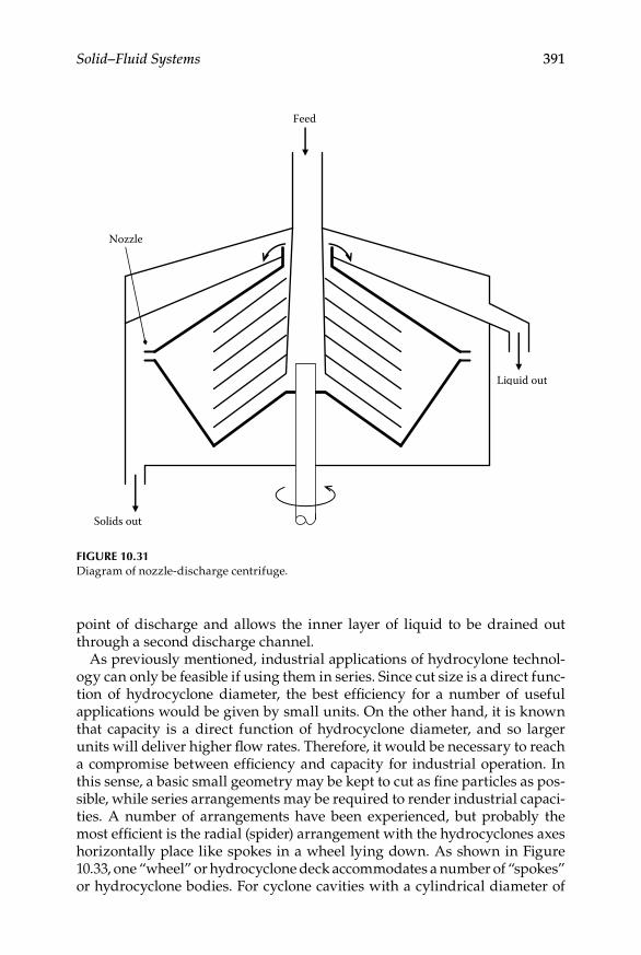
Solid–Fluid Systems 391
point of discharge and allows the inner layer of liquid to be drained out through a second discharge channel.
As previously mentioned, industrial applications of hydrocylone technol-ogy can only be feasible if using them in series. Since cut size is a direct func-tion of hydrocyclone diameter, the best efficiency for a number of useful applications would be given by small units. On the other hand, it is known that capacity is a direct function of hydrocyclone diameter, and so larger units will deliver higher flow rates. Therefore, it would be necessary to reach a compromise between efficiency and capacity for industrial operation. In this sense, a basic small geometry may be kept to cut as fine particles as pos-sible, while series arrangements may be required to render industrial capaci-ties. A number of arrangements have been experienced, but probably the most efficient is the radial (spider) arrangement with the hydrocyclones axes horizontally place like spokes in a wheel lying down. As shown in Figure 10.33, one “wheel” or hydrocyclone deck accommodates a number of “spokes” or hydrocyclone bodies. For cyclone cavities with a cylindrical diameter of
Solids out
Liquid out
Feed
Nozzle
Figure 10.31Diagram of nozzle-discharge centrifuge.

392 Unit Operations of Particulate Solids
10 mm the diameter of the deck is 300 mm. The whole cyclone deck can be molded by injection in one piece. The feed zone is the annular space closest to the periphery. The overflow is through peripheral screw-in-vortex finders. The underflow leaves via the central circular space where the small apex openings enter.
10.4.5.7 Laboratory Exercise: Efficiency of Hydrocyclone Separations
10.4.5.7.1 Introduction
Hydrocyclones can compete with centrifuges in clarification duties in diverse applications of the materials processing industries. Advantages of hydrocy-clone technology are: low cost, small space requirement, no moving parts, easy cleaning, and no need to use any aid for separation. Hydrocyclones are easily manufactured and modified and have been well tested in thickening, clarification, classification, and other operations in many industries. The best way to define efficiency of hydrocyclones is by determining the cut size at given conditions. The aim of the exercise is to evaluate the cut size in separating a suspension using a hydrocyclone.
10.4.5.7.2 Equipment and Materials
A hydrocyclone test rig comprising a sump, a small hydrocyclone unit (10–20 mm in diameter), recirculating piping system, valves, pressure gauge, and a centrifugal pump, can be used for the experiment. Routine laboratory material and glassware to carry out gravimetric testing, such as analytical balance, oven, desiccator, and sample containers, will be
Solids out Liquid out
Feed
Rotating conical drum
Rotating screw
Figure 10.32Principle of conveyor-bowl centrifuge.

Solid–Fluid Systems 393
sufficient for the test. The suggested material is fine limestone powder (median size 5–10 μm) to prepare a dilute suspension in water.
10.4.5.7.3 Instruments and Apparatuses
An instrumental particle size analyzer, such as a laser diffraction or electro sensing zone counter, will be appropriate options for measuring particle size distributions. A rotational viscometer will be used to measure apparent viscosity if the suspension results are non-Newtonian.
Feed
Collected overflows
Drain forunderflows
Collected underflows
Top view
Side view
“Spider” ofhydrocyclones
Drain for overflows
Figure 10.33Diagram of radial (spider) arrangement of hydrocyclones for industrial scale.

394 Unit Operations of Particulate Solids
10.4.5.7.4 Procedure
Prepare a suspension with a concentration of about 5% by volume of •fine calcium carbonate or similar powder in water.Run a test following the procedure described in Section 10.4.1.1. •Determine whether the suspension is Newtonian or not. If the sus-pension is non-Newtonian, derive the rheograms to determine parameters of characterization of the fluid.Determine the particle size distribution of feed using an instrumen-•tal particle sizer.Operate the hydrocyclone rig by filling the tank with the suspen-•sion. Start the pump with the recirculating valve fully open. Allow the suspension to recirculate for a few minutes to stabilize.Determine the flow rate of feed.•Open fully the valve for feed of the hydrocyclone. Slowly close the •recirculating valve until all the feed stream goes to the cyclone. With the recirculating valve fully closed and the hydrocyclone feeding valve fully open, the maximum pressure gauge reading will be the maximum pressure drop attainable. Register such pressure when is as stable as possible.Determine the flow rate of leaving streams from the hydrocyclone.•Carefully take a sample of the overflow and underflow simultane-•ously. Make two replicates of sampling.Determine gravimetrically the total efficiency of the separation •process.Determine the particle size distribution of overflow and underflow •streams with an instrumental particle sizer.
10.4.5.7.5 Calculations and Report
Following a procedure like the one described in Example 9.2, derive •the reduced grade efficiency curve for the separation process.From the curve, read off the cut size attained in the test.•Present a complete written report, according to scientific report •guidelines, either given by an instructor or consulted in the litera-ture. Include graphs, charts, and calculations carried out. Include analysis from own data and, as much as possible, discussion based on literature survey from studies and investigations on the subject.
10.4.6 Filtration
Filtration may be defined as the unit operation in which the insoluble solid component of a solid–liquid suspension is separated from the liquid

Solid–Fluid Systems 395
component by passing the suspension through a porous barrier which retains the solid particles on its upstream surface, or within its structure, or both. The solid–liquid suspension is known as the feed slurry or prefilt, the liquid component that passes through the membrane is called the filtrate and the barrier itself is referred to as the filter medium. The separated solids are known as the filter cake, once they form a detectable layer covering the upstream surface of the medium. The flow of filtrate may be caused by sev-eral means. Pressure and vacuum are two conventional ways of driving the suspension across the medium. Gravity and centrifugal forces may also be used for suspension medium crossing. In general terms, filtration theory applies to cases where cake buildup occurs.
10.4.6.1 Filtration Theory
In the initial stages of filtration the first particles of solid to encounter the filter medium become enmeshed in it, reducing its open surface area and increas-ing the resistance it offers to the flow of the filtrate. As filtration proceeds a layer of solids builds up on the upstream face of the medium and this layer, or cake, increase in thickness with time. Once formed, this cake in fact becomes the primary filtering medium. Filtrate passing through the filter encounters three types of resistance: a first resistance offered by channels of the filter itself, a second one because of the filter medium presence, and a third one due to the filter cake. The total pressure drop across the filter is equivalent to the sum of the pressure drops resulting from these three resistances. Usually, the pressure drop due to the channels of the filter is neglected in calculations. If −ΔP is the total pressure drop across the filter and −ΔPc and −ΔPm the pressure drops across the cake and medium respectively, then:
−ΔP = − ΔPc − ΔPm (10.88)
The pressure drop across the filter cake may be related to the filtrate flow by the expression (McCabe et al., 2005):
−∆ =
PwV
AVtc
dd
αµ2
(10.89)
where α is the specific resistance of the cake, μ is the viscosity of filtrate, w is the mass of solids deposited on the medium per unit volume of filtrate, V is the volume of filtrate, and A is the filter area normal to the direction of filtrate flow.
Alpha, α, physically represents the pressure drop necessary to give unit superficial velocity of filtrate of unit viscosity through a cake containing unit mass of solid per unit filter area. It is related to the properties of the cake by
α ε
ε ρ= −k S( )1 02
3s
(10.90)

396 Unit Operations of Particulate Solids
where k is a constant, ε is the porosity of the cake, S0 is the specific surface area of the solid particles in the cake, and ρs is the solids density.
If a cake is composed of rigid nondeformable solid particles α is indepen-dent of −ΔPc and does not vary throughout the depth of the cake, and is known as incompressible cake. However, if the cake contains nonrigid, deformable solid particles or agglomerates of particles the resistance to flow will depend on the pressure drop and will vary throughout the depth of the cake. In this case the cake is called compressible and an average value of the specific resis-tance for the entire cake must be used in Equation 10.89. This average specific resistance must be measured experimentally for any particular slurry.
By analogy with Equation 10.89 the filter medium resistance may be defined by the following relation:
− =
∆PR
AVtm
m dd
µ
(10.91)
where Rm is a constant known as the filter medium resistance.It is reasonable to assume that Rm is constant during any filtration cycle
and that it includes the resistance to filtrate flow offered by the filter channels. This being the case, Equations 10.88, 10.89, and 10.91 can be combined to give
dd m
Vt
A PwV A R
= −+
( )∆µ α
(10.92)
Equation 10.92 is a general expression for the filtrate flow rate.
10.4.6.2 Constant Pressure Filtration
When the pressure drop is maintained constant, Equation 10.92 may be integrated thus
d d dm
V V
tA P
wA
V V R Vt
= − +
∫ ∫ ∫µ α
( )∆0 0 0
(10.93)
or, substituting limits and transposing for time t:
t
Pw V
AR
VA
= −
+
µ α( )∆ 2
2
m
(10.94)
Equation 10.94 is a general expression for the filtration time during constant pressure filtration. In order to use it, values of α and Rm must
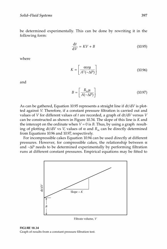
Solid–Fluid Systems 397
be determined experimentally. This can be done by rewriting it in the following form:
dd
tV
KV B= +
(10.95)
where
K
wA P
=−
α µ2 ( )∆
(10.96)
and
B
RA P
= −
mµ( )∆
(10.97)
As can be gathered, Equation 10.95 represents a straight line if dt/dV is plot-ted against V. Therefore, if a constant pressure filtration is carried out and values of V for different values of t are recorded, a graph of dt/dV versus V can be constructed as shown in Figure 10.34. The slope of this line is K and the intercept on the ordinate when V = 0 is B. Thus, by using a graph result-ing of plotting dt/dV vs V, values of α and Rm can be directly determined from Equations 10.96 and 10.97, respectively.
For incompressible cakes Equation 10.94 can be used directly at different pressures. However, for compressible cakes, the relationship between α and −ΔP needs to be determined experimentally by performing filtration runs at different constant pressures. Empirical equations may be fitted to
Filtrate volume, V
dt/d
V
B
Slope = K
Figure 10.34Graph of results from a constant pressure filtration test.
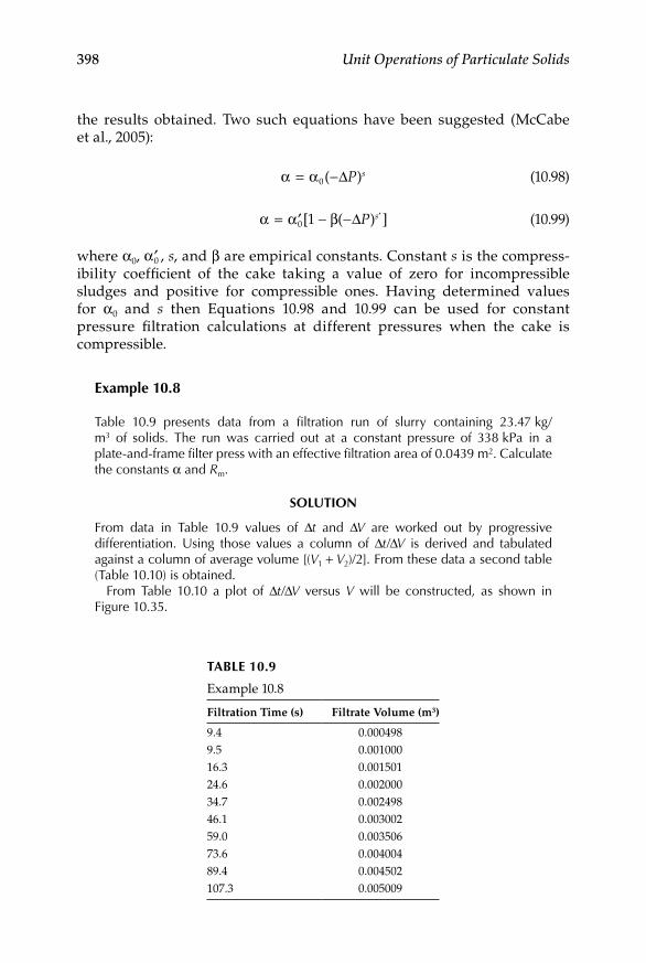
398 Unit Operations of Particulate Solids
the results obtained. Two such equations have been suggested (McCabe et al., 2005):
α α= −0( )∆P s (10.98)
α α β= ′ − − ′0 1[ ( ) ]∆P s
(10.99)
where α0, ′α0 , s, and β are empirical constants. Constant s is the compress-ibility coefficient of the cake taking a value of zero for incompressible sludges and positive for compressible ones. Having determined values for α0 and s then Equations 10.98 and 10.99 can be used for constant pressure filtration calculations at different pressures when the cake is compressible.
example 10.8
Table 10.9 presents data from a filtration run of slurry containing 23.47 kg/m3 of solids. The run was carried out at a constant pressure of 338 kPa in a plate-and-frame filter press with an effective filtration area of 0.0439 m2. Calculate the constants α and Rm.
SoluTion
From data in Table 10.9 values of Δt and ΔV are worked out by progressive differentiation. Using those values a column of Δt/ΔV is derived and tabulated against a column of average volume [(V1 + V2)/2]. From these data a second table (Table 10.10) is obtained.
From Table 10.10 a plot of Δt/ΔV versus V will be constructed, as shown in Figure 10.35.
Table 10.9
Example 10.8
Filtration Time (s) Filtrate Volume (m3)
9.4 0.0004989.5 0.00100016.3 0.00150124.6 0.00200034.7 0.00249846.1 0.00300259.0 0.00350673.6 0.00400489.4 0.004502107.3 0.005009

Solid–Fluid Systems 399
The graph in Figure 10.35 is a straight line with a correlation coefficient 0.997. The slope of such line (K) is 6 × 10⁶ s/m6, while the intercept with the y-axis (b) is 6352.4 s/m3. Transposing for α and Rm from Equations 10.96 and 10.97 respectively, the values of such constants are calculated as
α = ×( ) ( . ) ( )( . ) ( . )
6 10 0 0439 33800023 47 0 001
6 2s/m m kg/s mkg/m k
6 4 2
3 gg/ms1665267 1 m/kg
s/m m kg
11
m
3 2
= ×
=
.
( . ) ( . ) ( )
0
6352 4 0 0439 338000R
//s mkg/ms
9 4258 1 L/m2
1
( . ).
0 0010 0= ×
Table 10.10
Example 10.8
t (s) V (m3) Δt ΔV Δt/ΔV [(V1 + V2)/2]
0 09.4 0.000498 4.4 0.000498 8835 0.0002499.5 0.001000 5.1 0.000502 10159 0.00074916.3 0.001501 6.8 0.000501 13573 0.00125024.6 0.002000 8.3 0.000499 16633 0.00175034.7 0.002498 10.1 0.000498 20281 0.00224946.1 0.003002 11.4 0.000504 22619 0.00275059.0 0.003506 12.9 0.000504 25595 0.00325473.6 0.004004 14.6 0.000498 29317 0.00375589.4 0.004502 15.8 0.000498 31727 0.004253107.3 0.005009 17.9 0.000507 35306 0.004755
0
5000
10,000
15,000
20,000
25,000
30,000
35,000
40,000
0 0.001 0.002 0.003 0.004 0.005Filtrate volume (m3)
Λt/Λ
V (s/
m3 )
Figure 10.35Example 10.8.
400 Unit Operations of Particulate Solids
10.4.6.3 Constant Rate Filtration
If filtration is carried out at constant rate, then
ddVt
kVt
= =
(10.100)
Equation 10.100 may be rewritten as follows:
− =
+
∆PwV
A tV
VRAt
µα µ2
m
(10.101)
or
− = ′ + ′∆P K V B (10.102)
where
′ =
KwV
A tµα
2
(10.103)
and
′ =
BVRAt
µ m
(10.104)
Once again it can be seen that Equation 10.102 represents a straight line if −ΔP is plotted against V. The slope of the line is K′ and the intercept to the y-axis when V = 0 is B′. Thus, for incompressible cakes α and Rm can again be determined by experimental means.
For compressible cakes, the relationship between α and −ΔPc must, again, be experimentally determined. If a relationship of the form shown in Equation 10.98 is assumed to apply, then Equation 10.89 may be modified to
( ) [ ( )]− = − − =− −∆ ∆ ∆P P P
wVA
Vt
s sc m
01 12
µα
(10.105)
which, in turn may be written as
[ ( )]− − = ′′−∆ ∆P P K tsm
1 (10.106)

Solid–Fluid Systems 401
where
′′ =
Kw
AVt
µα02
2
(10.107)
If it is assumed that −ΔPm is constant throughout a constant-rate filtration then by plotting t versus −ΔP and passing a smooth curve through the points and extrapolating the curve to the y-axis, an approximate value for −ΔPm can be obtained. If −(ΔP − ΔPm) is then plotted against t on log–log paper and a straight line is obtained, the slope of this line is (1 – s). Thus, s can be calculated and K″ and α0 can be derived from Equations 10.106 and 10.107. When the first log–log plot of −(ΔP − ΔPm) is not a straight line; further approximations for −ΔPm need to be made (McCabe et al., 2005).
example 10.9
Calculate the volume obtained, and the time required in reaching such volume, in a constant-rate filtration process keeping a rate of 0.05 m3/min until the pressure drop reaches 250 kN/m2, according to data in Table 10.11.
SoluTion
For constant rate filtration, plotting directly −ΔP versus V, the graph shown in Figure 10.36 is obtained.
The correlation parameters of the slope line represented in Figure 10.36 are: K′ = 490 and B′ = 15.5, with a correlation coefficient of 0.9971. The equation rep-resenting the particular straight line in Figure 10.36 is, thus
− = +∆P V490 15 5.
Substituting the value of 250 kPa in the above equation and transposing for V, the volume at that maximum attained pressure is: V = 0.4878 m3.
Since time in Table 10.11 shows the same linear trend than pressure drop and volume, for the pressure drop of 250 kPa the approximate time is t = 8.92–9 min.
Table 10.11
Example 10.9
t (min) −ΔP (kN/m2) V (m3)
0 0 0.001 40 0.052 65 0.103 90 0.154 110 0.205 140 0.25

402 Unit Operations of Particulate Solids
10.4.6.4 Filtration Media and Filter Aids
Filtration equipment is adapted with consumable materials for every partic-ular duty. The main consumables in diverse filtration operations are the fil-tering medium and the filter aids. Filter media are selected, primarily, in function of the pore size that will be appropriate for retention of the solids in suspension. Other important functions of the filtering medium are the promotion of cake formation and the support of cake once formed. The medium should offer minimum resistance to flow accordingly to the need of a rapid formation of the filter cake. It must be strong enough to support the cake and retain its strength under the extreme conditions that may occur during operation. The surface characteristics of the filtering medium should facilitate cake removal. It must be nontoxic and chemically compatible with materials being filtered, and also it should be cost effective. Filter media may be rigid or flexible. Rigid media may be loose or packed. Examples of loose rigid media are sand, gravel, diatomaceous earths, and charcoal. Packed or fixed rigid media include porous carbon, porcelain, fused alumina, perfo-rated metal plates, or rigid wire mesh. Flexible media may comprise woven fabrics of cotton, silk, wool, and jute. Flexible media made out of synthetics include nylon, polypropylene, polythene, polyvinylchloride, and copoly-mers. Glass fiber and flexible metal meshes are also used as filter media, as well as nonwoven materials, such as cotton fibers, wool fibers, and paper pulp. These materials may be available in preformed pads of various shapes. Table 10.12 summarizes different filtering materials along with their main features. Some other characteristics, such as the woven pattern and the geometric dimensions of the fibers, are considered selection criteria and can be presented in tabular form (Clark, 1990).
0
20
40
60
80
100
120
140
160
0 0.05 0.1 0.15 0.2 0.25 0.3Filtrate volume (m3)
Pres
sure
dro
p (k
Pa)
Figure 10.36Example 10.9.
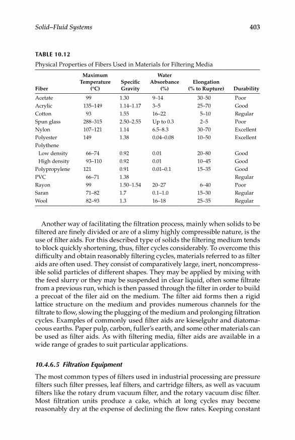
Solid–Fluid Systems 403
Another way of facilitating the filtration process, mainly when solids to be filtered are finely divided or are of a slimy highly compressible nature, is the use of filter aids. For this described type of solids the filtering medium tends to block quickly shortening, thus, filter cycles considerably. To overcome this difficulty and obtain reasonably filtering cycles, materials referred to as filter aids are often used. They consist of comparatively large, inert, noncompress-ible solid particles of different shapes. They may be applied by mixing with the feed slurry or they may be suspended in clear liquid, often some filtrate from a previous run, which is then passed through the filter in order to build a precoat of the filer aid on the medium. The filter aid forms then a rigid lattice structure on the medium and provides numerous channels for the filtrate to flow, slowing the plugging of the medium and prolonging filtration cycles. Examples of commonly used filter aids are kieselguhr and diatoma-ceous earths. Paper pulp, carbon, fuller’s earth, and some other materials can be used as filter aids. As with filtering media, filter aids are available in a wide range of grades to suit particular applications.
10.4.6.5 Filtration Equipment
The most common types of filters used in industrial processing are pressure filters such filter presses, leaf filters, and cartridge filters, as well as vacuum filters like the rotary drum vacuum filter, and the rotary vacuum disc filter. Most filtration units produce a cake, which at long cycles may become reasonably dry at the expense of declining the flow rates. Keeping constant
Table 10.12
Physical Properties of Fibers Used in Materials for Filtering Media
Fiber
Maximum Temperature
(°C)Specific Gravity
Water Absorbance
(%)Elongation
(% to Rupture) Durability
Acetate 99 1.30 9–14 30–50 PoorAcrylic 135–149 1.14–1.17 3–5 25–70 GoodCotton 93 1.55 16–22 5–10 RegularSpun glass 288–315 2.50–2.55 Up to 0.3 2–5 PoorNylon 107–121 1.14 6.5–8.3 30–70 ExcellentPolyester 149 1.38 0.04–0.08 10–50 ExcellentPolythene
Low density 66–74 0.92 0.01 20–80 GoodHigh density 93–110 0.92 0.01 10–45 Good
Polypropylene 121 0.91 0.01–0.1 15–35 GoodPVC 66–71 1.38 RegularRayon 99 1.50–1.54 20–27 6–40 PoorSaran 71–82 1.7 0.1–1.0 15–30 RegularWool 82–93 1.3 16–18 25–35 Regular

404 Unit Operations of Particulate Solids
rate filtration is costly as the pressure drop must be increased during the cycle.
A commonly used design of filter press is the plate-and-frame filter press. The components of a plate-and-frame filter press are the frames and the two types of grooved plates, filter plate and wash plate, shown in Figure 10.37a. The grooved plates covered on both sides with filter medium and alterna-tively assembled with frames, as illustrated in Figure 10.37b, are mounted in a rack. The whole assembly can be squeezed tightly together by a screw driven manually or by a hydraulic or pneumatic mechanism, to form a liquid tight unit (Figure 10.38). Both plates and frames are provided with openings
Filtrate out
FPFP F FWPM M M
Feed
FPFP FF WPM M M
Wash liquid
Closed outlet Washings out Washings out
Wash plate Frame Filter plate
(a)
(b)
(c)
FP: Filter plateF: Frame M: Medium WP: Wash plate
Figure 10.37Description and arrangements of filter press components: (a) detail of plates and frames, (b) arrangement for the filtration cycle, and (c) arrangement for the washing cycle.

Solid–Fluid Systems 405
at one corner, so that when the press is closed these openings form a channel through which the feed is introduced. Slurry is fed into the frames and the cake builds up in the hollow center of the frames. The filtrate passes through the medium and to the grooved surfaces of the filter plates to be removed via an outlet channel in each plate. Filtration continues until the flow of filtrate drops below a practical level, or when accumulation of cake in the frames elevates pressure to an extremely high level. Washing of the cake can be car-ried out by replacing the flow of feed slurry with wash liquid or by the use of special wash plates mounted in the arrangement so that every second plate is a wash plate. On running a filtration cycle these wash plates act as filter plates, while during washing their outlets are closed and the wash liquid is introduced to their surfaces through a special inlet channel. The flow path for both filtration and washing cycles using wash plates is illustrated in Figure 10.37b and c, respectively.
Another alternative of pressure filtration are pressure-vessel filters that make use of filter leaves as the basic filter element. A filter leaf consists on a wire mesh screen or grooved drainage plate over which the filter medium is stretched. The leaf may be suspended from the top or supported from the bottom or center. The supporting element is usually hollow and forms an outlet channel for the filtrate. Several designs of pressure-vessel filters with filter leaves elements are commercially available. Two of them are the hori-zontal-leaf filter and the vertical-tank vertical-leaf filter, both shown in Figure 10.39. Vertical-tank vertical-leaf filters (Figure 10.39a) are the cheapest of the pressure leaf-filters and have the lowest volume-to-area ratio. Cake discharge is accomplished by sluicing, either manually or by vibration. Horizontal-leaf
FeedFixed plate Filter medium
Plates and frames
Supporting rail
Screw
Filtrate out
Figure 10.38Schematic diagram of a plate-and-frame filter press assembled and mounted.

406 Unit Operations of Particulate Solids
filters (Figure 10.39b), in either a horizontal or vertical tank, are advantageous when the flow is intermittent. Filtration takes place only on the upper size of the horizontal leaves, and so filtration area is limited compared with other pressure-vessel designs. Horizontal-leaf filters are most suitable when thor-ough cake washing is necessary. Cake discharge may be accomplished by rotation of the leaves.
In vacuum filters a subatmospheric pressure is maintained downstream of the medium while an atmospheric one is kept upstream. Because the pres-sure drop across the filter is limited to one atmosphere, they are not suited to batch operations. Some types of leaf filters, tube filters, or edge filters can be operated under vacuum, but continuous vacuum filters are far most com-mon. Since the upstream pressure is atmospheric, cake discharge is facili-tated thus favoring continuous operation. The rotary drum vacuum filter is, perhaps, the most common type of vacuum equipment used in an important number of applications. As can be seen in Figure 10.40a, vacuum is applied to the inside of a revolving drum covered with reinforced wire mesh and filtering cloth or medium. The surface of the drum consists of a number of shallow compartments formed between dividing strips running the length of the drum. Each compartment is connected by one or more pipelines to an
Feed
Filtrate
FiltrateDrain
Wash liquid
Vertical leaf filters
Horizontal leaf filters
Collectingplates
(a) (b)
Figure 10.39Pressure-vessel leaf filters: (a) vertical-tank, vertical-leaf filter, and (b) horizontal-leaf filter.

Solid–Fluid Systems 407
automatic rotary valve situated centrally at one end of the drum. Filtering medium covers the entire drum surface and is supported by perforated plates, grids, or wire mesh to provide drainage space between the medium and the floor of each shallow compartment. The drum dips into slurry and rotates, a vacuum is drawn on its surface and filtrate flows through the medium and out through the drain pipe from the compartment and is directed to the filtrate receiver by means of the valve. A layer of cake builds up on the outer surface of the medium and the cake is sucked free from the filtrate as the drum turns becoming dryer near the end of the turn. Prior to be submerged again in the slurry tank in completing a drum revolution, a knife removes the cake in the form of a continuous layer. Rotary vacuum
Feed slurry
Suction
Trunnion
Hollowdrum
Internal piping
Support and filtering medium
Drumsurface
Cake
Knife
(a)
(b)
Feed slurry
Suction
Filter discs
Scraper knives
Figure 10.40Equipment for vacuum filtration: (a) continuous rotary drum, and (b) rotary disc.

408 Unit Operations of Particulate Solids
precoat filters may produce filtrates which would contain 0.1% or less suspended solids. Rotary vacuum disc filters (Figure 10.40b) consist of a number of circular filter leaves mounted on a horizontal axis about which they rotate. Each disc is fitted with a cake removal device and is divided into sectors, each of which has an individual outlet to the central shaft. These outlets form a continuous channel through which the filtrate flows from all sectors at the same angle. All the channels terminate in a rotary valve like the one used in drum filters. In operation each disc operates as a drum filter, with the cycle being controlled by the rotary valve.
10.4.6.6 Laboratory Exercise: Filtration Curves Using a Filter Press
10.4.6.6.1 Introduction
Filtration is a unit operation with diverse applications in the materials pro-cessing industries. The mode normally used in industrial filtration is cake filtration in which solids build up on the surface of a filtering medium, its accumulation known as cake. The factor used to make pass the filtrate through the cake and the medium can be pressure force or vacuum force. Pressure is used in an important number of equipment. The pressure drop is maintained constant in the filtration mode referred to as constant pressure filtration. In this mode of filtration the flow rates decline as the filtration cycle progresses. Another mode of filtration is constant rate filtration, in which the flow rates do not decline for a given cycle. Constant pressure filtra-tion is, normally, more convenient because constant rate filtration is costly as the pressure drop must be increased during the cycle. A common piece of filtration equipment in numerous processing applications is the plate-and-frame filter press. Any type of pressure-vessel filter normally requires filter aids to facilitate cake formation and a trouble-free operation. Some types of biological slurries, such as nonclarified fruit juices, tend to form a cake rela-tively easy without need of filter aids due to the pectinaceous nature of the suspended solids.
The objective of the experiment is to run a plate-and-frame filter press in constant pressure mode in order to determine the filtration plot describing a filtration cycle, and calculate the empirical constants of cake resistance and filter medium resistance.
10.4.6.6.2 Equipment and Materials
A laboratory size filter press rig comprising tank, pipeline, centrifugal pump, filter plates, valves, and pressure gauges. Domestic juice extractor and uten-sils of a food processing plant, such as knives, apple corer, containers, and so on. Routine laboratory material and glassware to carry out gravimetric testing, such as analytical balance, oven, desiccator, and sample containers, will be sufficient for the test. A batch of second-grade apples suitable for juice extraction is the suggested raw material.
Solid–Fluid Systems 409
10.4.6.6.3 Procedure
Use a batch of apple sufficient to prepare about 10 L of nonclarified •juice.Weigh the apples, wash them, core them, and peel them.•Extract the juice until obtaining the approximate 10-L sample.•Take an aliquot of the juice sample and determine, gravimetrically, •its total solids content.Mount the filter press arrangement checking for leaks.•Fill up the filter tank, record the volume.•Open the filter feeding and the recirculating valves.•Recirculate the suspension for 10 min.•Stabilize the pressure gauge reading at 150 kPa, approximately.•Open the valve of filtrate and close the valve of recirculation •simultaneously.Take filtrate samples for 10 min, until the volume in the tank comes •to a minimum.Verify the total volume of filtrate obtained.•Drain the remaining liquid and clean the rig rigorously.•
10.4.6.6.4 Calculations and Report
Analyze the data collected following the procedure of Example 10.8, •that is, derive a table like Table 10.10.Plot the data from the table obtained, and verify if they fit a straight •line. If the linearity is confirmed, obtain the equation fitting the data from the regression model and determine the parameters.Calculate • α and Rm from the obtained values of the slope K and the intercept B.Present a complete written report, according to scientific report •guidelines, either given by instructor or consulted in the literature. Include graphs, charts, and calculations carried out. Include analysis from own data and, as much as possible, discussion based on litera-ture survey from studies and investigations on the subject.
10.4.7 other Techniques: Membrane Separations
Membrane separations are techniques used industrially for removal of sol-utes and emulsified substances from solutions by application of pressure onto a very thin layer of a substance with microscopic pores, known as a membrane. Membrane separation processes include reverse osmosis (RO), ultrafiltration (UF), microfiltration (MF), dialysis, electrodialaysis, gas
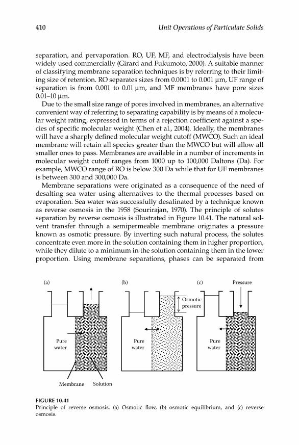
410 Unit Operations of Particulate Solids
separation, and pervaporation. RO, UF, MF, and electrodialysis have been widely used commercially (Girard and Fukumoto, 2000). A suitable manner of classifying membrane separation techniques is by referring to their limit-ing size of retention. RO separates sizes from 0.0001 to 0.001 μm, UF range of separation is from 0.001 to 0.01 μm, and MF membranes have pore sizes 0.01–10 μm.
Due to the small size range of pores involved in membranes, an alternative convenient way of referring to separating capability is by means of a molecu-lar weight rating, expressed in terms of a rejection coefficient against a spe-cies of specific molecular weight (Chen et al., 2004). Ideally, the membranes will have a sharply defined molecular weight cutoff (MWCO). Such an ideal membrane will retain all species greater than the MWCO but will allow all smaller ones to pass. Membranes are available in a number of increments in molecular weight cutoff ranges from 1000 up to 100,000 Daltons (Da). For example, MWCO range of RO is below 300 Da while that for UF membranes is between 300 and 300,000 Da.
Membrane separations were originated as a consequence of the need of desalting sea water using alternatives to the thermal processes based on evaporation. Sea water was successfully desalinated by a technique known as reverse osmosis in the 1958 (Sourirajan, 1970). The principle of solutes separation by reverse osmosis is illustrated in Figure 10.41. The natural sol-vent transfer through a semipermeable membrane originates a pressure known as osmotic pressure. By inverting such natural process, the solutes concentrate even more in the solution containing them in higher proportion, while they dilute to a minimum in the solution containing them in the lower proportion. Using membrane separations, phases can be separated from
Solution Membrane
(a) (b) (c)
Purewater
Purewater
Purewater
Osmotic pressure
Pressure
Figure 10.41Principle of reverse osmosis. (a) Osmotic flow, (b) osmotic equilibrium, and (c) reverse osmosis.

Solid–Fluid Systems 411
two-phase and multiphase systems without the need of any phase state change, that is, without requiring thermal energy. The osmotic pressure π for dilute solutions can be established as a function of pressure and tempera-ture, using fundamental thermodynamics, as follows:
π = MRT (10.108)
where M is the molar concentration of the solution, R the universal gas constant, and T the absolute temperature.
UF is often compared with RO although the mechanism of separation is quite different. This difference is illustrated in Figure 10.42. As can be seen, in RO a rejection is based on electrostatic repulsion due to formation of a pure layer of water over the membrane, and the virtual charges on this layer reject charges of ionic free species of salt solutions (Figure 10.42a). Simultaneously, by a complex mechanism of sorption, diffusion, and desorp-tion, pure water passes through the membrane performing the separation
+AnionCation
Water monolayer
Nonporousmembrane
+-+-+-+-+-+-+-+-+-+-+-+-+-+-+-+-+-+-+-+-+-+-+-+-+-+-+-+-
–
Water
(a)
+ Macromolecule
H2O H2O
Porousmembrane
__Anion
Cation
(b)
Figure 10.42Rejection mechanisms for (a) reverse osmosis and (b) ultrafiltration.
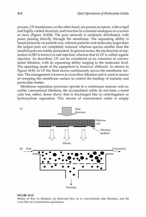
412 Unit Operations of Particulate Solids
process. UF membranes, on the other hand, are porous in nature, with a rigid and highly voided structure, and function in a manner analogous to a screen or sieve (Figure 10.42b). The pore network is randomly distributed, with pores passing directly through the membrane. The separating ability is based primarily on particle size, wherein particles and molecules larger than the largest pore are completely retained, whereas species smaller than the smallest pore are totally permeated. In general terms, the mechanism of sep-aration in RO is known as salt rejection, whereas that in UF is called organic rejection. As described, UF can be considered as an extension of conven-tional filtration, with its separating ability ranging to the molecular level. The operating mode of the equipment is, however, different. As shown in Figure 10.43, in UF the fluid moves continuously across the membrane sur-face. The arrangement is known as cross-flow filtration and is used as means of sweeping the membrane surface to control the buildup of foulants and particulate matter.
Membrane separation processes operate in a continuous manner and so, unlike conventional filtration, the accumulated solids do not form a moist cake but, rather, dense slurry that is discharged like in centrifugation or hydrocyclone separation. This stream of concentrated solids is simply
Feed Concentrate
Permeate
Flow direction
Filtrationcake
Filtration medium
Filtrate
(a)
(b)
Figure 10.43Modes of flow in filtration: (a) dead-end flow as in conventional cake filtration, and (b) cross-flow as in membrane separations.

Solid–Fluid Systems 413
known as concentrated while the clarified stream is called permeate. A schematic flow diagram of UF and some other membrane separations is shown in Figure 10.44. The flow rate Q through a membrane separation process may be represented by
Q kA P= −( )∆ ∆π (10.109)
where k is a membrane permeability coefficient, A is the membrane super-ficial area, ΔP is the pressure drop, and Δπ the difference in osmotic pressure between the feed and the permeate. Equation 10.109 is more suitable for RO applications, due to the osmotic pressure exerted by solutes in such a pplications. For UF applications Δπ is negligible in relation to ΔP and the membrane thickness causes an effect in the process, and so it should be included as a variable. Under these considerations, Equation 10.109 can be reexpressed as
Q
kAP=
δ ∆
(10.110)
where δ is the membrane thickness.The pressure drop ΔP in Equation 10.110 is, really, an average pressure or
pressure gradient due to the cross-flow arrangement of membrane separa-tion processes. Referring to Figure 10.40, a feed stream containing differently size solids is pumped across the membrane surface at a velocity determined by the feed side pressure gradient (P1 – P2). This gradient, known as hydrody-namic pressure gradient, causes the continuous movement of fluid across the membrane that is referred to as cross-flow. As the feed stream flows across the membrane surface, smaller particles may be able to pass through the membrane and exit in the permeate stream (Figure 10.43) at a pressure P3, which is usually atmospheric. The rate of permeate flow is generally reported as flux, that is, flow rate per unit area of membrane. The driving force for
Feed:Q(F )
XFP1
Concentrate:CXcP2
Permeate(Filtrate):
FXpP3
Figure 10.44Mass balance in a membrane separation process.

414 Unit Operations of Particulate Solids
permeate flow is also a pressure gradient, but is not the hydrodynamic pres-sure gradient defined above. Instead, is the pressure gradient that exits through the membrane, from feed size to permeate size, at each point along the membrane surface. This pressure gradient is known as the transmem-brane pressure gradient or simply transmembrane pressure (TMP). Clearly, TMP varies along the membrane surface being a maximum at the inlet and a minimum at the outlet. An average TMP, according to the diagram in Figure 10.40, can be defined as
TMP = + −P P
P1 232
(10.111)
The permeate pressure P3 is negligible as compared with the pressure gradi-ent between feed and concentrate and, thus
TMP = +P P1 2
2 (10.112)
A way of expressing efficiency of a membrane separation process is by deter-mining a recovery percentage as the relation of the permeate flow rate to the feed flow rate (Figure 10.44), that is,
% ( )Recovery = F
Q 100
(10.113)
Recovery percentages depend on the feed concentration, being higher at lower concentrations of feed solids. A fraction of liquid, approximately equal to that of solids, should remain in the concentrate to make it flow. Therefore, as illustrated in Figure 10.45, the most diluted the feed, the higher the per-centage of recovery.
Membranes for UF and similar processes are made out of a very thin film with microperforations of 0.1–1 μm size. Such tiny perforation on quite a thin film would be easily damaged by the applied pressures needed to perform separation in actual operation. The ultrathin skin or film is, therefore, sup-ported on a relatively thick (100–200 μm thick) substructure. The retention is performed over the thin film, on which the pore sizes may vary due to the manufacturing technique. Two common membrane structures are the plane membrane and the hollow fiber membrane, illustrated in Figure 10.46.
Over the years, four generations of membrane materials have been appeared in the market. The first generation comprised cellulosic materials, the second included polymeric materials, the third was mainly from inor-ganic materials, and the fourth is based on carbon fibers. Conventional nomenclature of UF membranes includes two prefix letters (e.g., UM, PM, and XM) that refer to different polymers, and two last digits which indicate
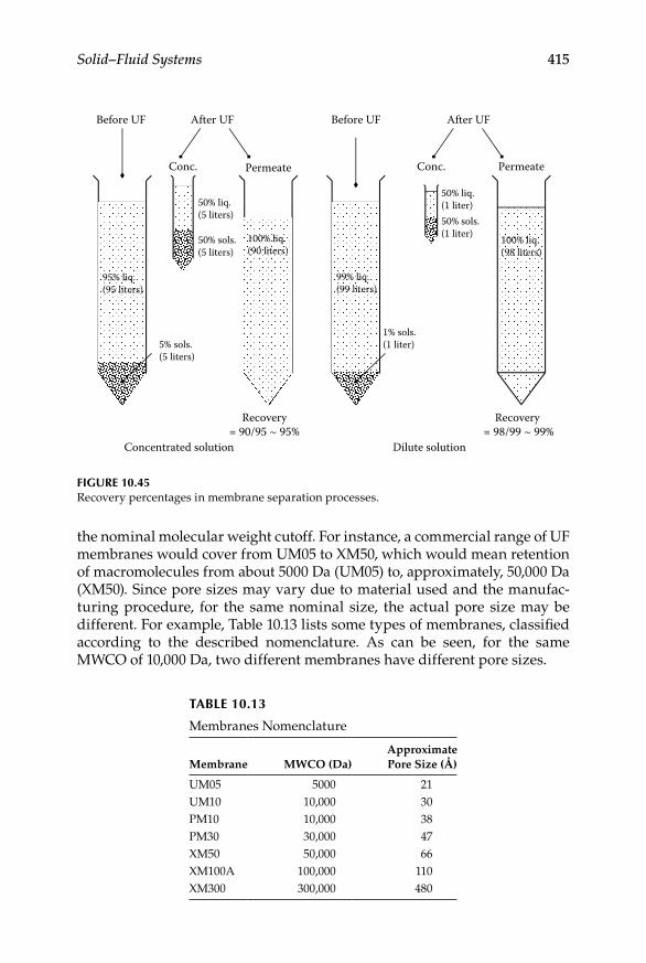
Solid–Fluid Systems 415
the nominal molecular weight cutoff. For instance, a commercial range of UF membranes would cover from UM05 to XM50, which would mean retention of macromolecules from about 5000 Da (UM05) to, approximately, 50,000 Da (XM50). Since pore sizes may vary due to material used and the manufac-turing procedure, for the same nominal size, the actual pore size may be different. For example, Table 10.13 lists some types of membranes, classified according to the described nomenclature. As can be seen, for the same MWCO of 10,000 Da, two different membranes have different pore sizes.
Before UF
95% liq.(95 liters)
5% sols.(5 liters)
50% liq. (5 liters)
50% sols. (5 liters)
After UF
Conc.
100% liq. (90 liters)
Recovery = 90/95 ~ 95%
Recovery = 98/99 ~ 99%
100% liq. (98 liters)
Before UF After UF
Conc. Permeate
99% liq. (99 liters)
1% sols. (1 liter)
50% liq. (1 liter) 50% sols. (1 liter)
Dilute solution Concentrated solution
Permeate
Figure 10.45Recovery percentages in membrane separation processes.
Table 10.13
Membranes Nomenclature
Membrane MWCO (Da)Approximate Pore Size (Å)
UM05 5000 21UM10 10,000 30PM10 10,000 38PM30 30,000 47XM50 50,000 66XM100A 100,000 110XM300 300,000 480
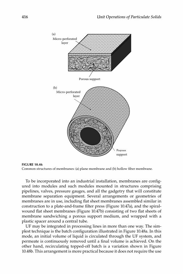
416 Unit Operations of Particulate Solids
To be incorporated into an industrial installation, membranes are config-ured into modules and such modules mounted in structures comprising pipelines, valves, pressure gauges, and all the gadgetry that will constitute membrane separation equipment. Several arrangements or geometries of membranes are in use, including flat sheet membranes assembled similar in construction to a plate-and-frame filter press (Figure 10.47a), and the spiral-wound flat sheet membranes (Figure 10.47b) consisting of two flat sheets of membrane sandwiching a porous support medium, and wrapped with a plastic spacer around a central tube.
UF may be integrated in processing lines in more than one way. The sim-plest technique is the batch configuration illustrated in Figure 10.48a. In this mode, an initial volume of liquid is circulated through the UF system, and permeate is continuously removed until a final volume is achieved. On the other hand, recirculating topped-off batch is a variation shown in Figure 10.48b. This arrangement is more practical because it does not require the use
Micro-perforatedlayer
Porous support
orated
Micro-perforated layer
Poroussupport
perforatedlayer
Poroussupport
(a)
(b)
Figure 10.46Common structures of membranes: (a) plane membrane and (b) hollow fiber membrane.

Solid–Fluid Systems 417
of a large feed tank and allows the specification of a smaller prefilter prior to the system.
example 10.10
Calculate the pressure drop needed to maintain a water flow rate of 15 mL/cm2 min in a process of desalting sea water by RO at room temperature. The water contains 35 g/L of solids and the coefficient of permeability of the membrane can be taken as 1.125 × 10⁻⁴ cm/mm Hg min.
Feed
Permeate
Concentrate
(a)
PermeateCollect pipe
Feed
Feed
Cover
Feed flow
Spacer
Spacer
Membrane
Concentrate
Concentrate
(b)
Figure 10.47Membrane modules for assembly into equipment: (a) plate-and-frame arrangement and (b) spiral-wound arrangement.

418 Unit Operations of Particulate Solids
SoluTion
The osmotic pressure of the solution can be calculated using Equation 10.108, where molarity of salt is approximately 0.6 and at room temperature (298 K) the value of the universal gas constant is R = 0.08205 l atm/K mol. Substituting, thus, into Equation 10.108:
π = = ≈( . )( . )( ) .0 6 0 08205 298 14 67 atm 11172 mm Hg
The water flow rate is, indeed, a flux of water since it includes the area. Flux can be defined as: J = Q/A. On the other hand, since the osmotic pressure of the per-meate approaches zero, Δπ is, simply, the osmotic pressure π, calculated above. Taking into account these arguments, transposing for ΔP in Equation 10.109, and substituting values:
∆PJk
= + = + = ×π 15 cm /cm min0.0001125 cm/mmHgmin
mmHg 14451 13 2
11172 . 005 mmHg
Concentrate
Permeate
Membranemodules
(a)
Concentrate
Membranemodules
(b)
Figure 10.48Diagram of membrane separation operation modes: (a) standard batch configuration and (b) topped-off batch system with recirculation loop.

Solid–Fluid Systems 419
The pressure drop needed to maintain the required capacity is, thus: ΔP ~ 19,400 kPa.
10.4.8 Dimensionless Scale-up of equipment
Optimization, adaptation, and innovation of industrial operations involving solid–liquid separations are based, like many other industrial processes, in laboratory experimentation followed by pilot plant testing and finishing with scale-up of equipment to establish a production line. Selection and sizing of equipment for solid–liquid separations is still a complex process requiring expert knowledge and expertise, and supported on testing on the actual system to be processed. Fundamentals play, also, an important role in the overall exercise of scaling-up procedures and, along with the expertise and testing, should render satisfactory results as to adjust theoretical calculations with real processing. This section reviews some basic theoreti-cal principles useful for preliminary selection and sizing of solid–liquid separation equipment, in the most frequently employed categories.
Sizing of dynamics separators whose separation principle is governed by gravity or centrifugal forces may be easily scaled using dimensionless groups, providing the feed suspension is nonflocculating or the flocculation is completed prior to feeding of the suspension to the separator. The most relevant dimensionless groups for separators using gravitational or centrifu-gal forces that have been already described, discussed, and utilized in this book are the Reynolds number Re relating the inertial and viscous forces in a pocket of fluid, the Euler number Eu describing the resistance of a separa-tor to flow, the Stokes number Stk relating the inertial and viscous forces on a particle, and the Froude number Fr relating the inertial and gravitational forces in a particle. In a form, more generic than the one used in this book, the Stokes number is represented by
Stk = τv
D (10.114)
An expression for the Froude number is
Fr
gDv
= 2 (10.115)
In the Stokes number relationship τ is the particle relaxation time defined as
τ ρ ρ
µ= −x2
18( )s
(10.116)
In Equations 10.114 through 10.116 the components have already been defined, that is, v is the characteristic velocity of flow in the separator, D is
420 Unit Operations of Particulate Solids
the characteristic linear dimension of the separator, g is the acceleration due to gravity, x is the equivalent Stokes diameter, ρs is the solids density, ρ is the liquid density, and μ is the liquid viscosity.
In gravity settling tanks, assuming low feed solids concentration and plug flow through a vessel of plan area A, the following relationship for its grade efficiency can be derived:
G x( ) = ⋅Stk Fr (10.117)
where the characteristic velocity is: v = Q/A, while Q is the volumetric flow rate and D is the height of the settling tank.
If x is the cut size x50, then G(x) = 0.5, and the above equation becomes
Q u A= 2 g (10.118)
where ug is the terminal settling velocity under gravity, of the cut size x50 from Stokes law:
u
x gg
s=−50
2
18( )ρ ρ
µ (10.119)
Equation 10.119 represents the very best performance of a settling tank. Such performance should be considered theoretical or ideal, and so it may not be totally applicable due to nonideal distribution of the flow, end effects, turbu-lence, and some others effects. However, it can be used as a preliminary approach to select the minimum area of the tank required to obtain a given cut size.
The sedimentation process in centrifugal devices is somewhat similar to sedimentation under gravity, except that the settling is radial and not paral-lel. A plug-model for the flow through the wall of the centrifuge leads to an exponential equation for the grade efficiency. For the cut size x50, this men-tioned equation would reduce to Equation 10.118 but with the area A replaced by a factor Σ. Such an equation is, in fact, Equation 10.74, the so-called Sigma theory equation. As mentioned when presenting such equa-tion, factor Σ has a dimension of area and is calculated for the geometry of a particular centrifuge, so that each type of centrifuge has its own equation. Extensive work on the Sigma theory has shown that, while experimental results differ from calculated values when different centrifuges are consid-ered, the scale-up between centrifuges of the same type is fairly reliable. This is based on a simple application of Equation 10.74 when a laboratory experi-ment with a small centrifuge 1 is compared with a larger scale operation on a larger centrifuge 2, of the same type and with the same slurry. For a case such as this, the following relation may apply:
Q Q1
1
2
2Σ Σ=
(10.120)

Solid–Fluid Systems 421
When Equation 10.120 holds, the cut size and the overall separation efficiency, in both cases, should be the same. Equation 10.120 can be used for sizing centrifuges from laboratory tests, or for predicting capacities of existing machines.
example 10.11
A centrifugal clarification system is used to eliminate settling solids from liquor resulting after a fermentation process. The solids have a density of 2650 kg/m3 and are suspended in water at a very low concentration. In laboratory tests it has been found that a satisfactory clarity with a sigma value of 220 m2 and a capacity of 8 × 10⁻⁶ m3/s. If a larger centrifuge is used, with a sigma value of 2500 m2 for large-scale operation: Which capacity will the new operation have? Which will be the effective cut size for that new capacity?
SoluTion
Taking the values from laboratory testing as Σ1 and Q1, substituting directly into Equation 10.120, and transposing for Q2:
Q Q2
2
11
62500220
8 10 0 0=
= × = ×− −Σ
Σm
mm /s 9 9 1 m /s
2
23 5 3( ) .
The cut point can be obtained by substituting either set of values, that is, Q1 and Σ1 or Q2 and Σ2, into Equation 10.74 and transposing for xc. Using, thus, Q1 and Σ1 values and substituting in Equation 10.74, transposed for xc:
xc
3
3 2 2
kg/ms m /skg/m m/s m
= × −18 0 001 8 1021650 9 81 220
6( . ) ( )( ) ( . ) ( )
= × −
1 2
71 42 10/
. m
Therefore, the industrial capacity is 9 × 10⁻⁵ m3/s, approximately and the cut size is about 0.14 μm.
For the case of centrifugal separation using hydrocyclones, at low solids concentrations (<1 or 2% by volume) the flow pattern in them is practically unaffected by the presence of particles, and so particle–particle interaction is negligible. The volume of the particles being separated into the underflow is small and the underflow-to-throughput ratio Rf is usually assumed to have no effect on the cut size x50. The minimum effect of flow splitting can be easily compensated by using the reduced efficiency concept, as previously discussed. Dimensional analysis, coupled with fundamental theories of separation in hydrocyclones, gives two relationships between the three dimensionless groups Re, Eu, and Stk:
Stk Eu constant′ =50 (10.121)

422 Unit Operations of Particulate Solids
Eu = k n(Re) (10.122)
where k and n are empirical constants for a family of geometrically similar hydrocyclones, while Stk′50 is the Stokes number for the reduced cut size ′x50 determined from the reduced grade efficiency G′(x) in Equation 10.29. The characteristic linear dimension is the diameter of the cylindrical part of the hydrocyclone and the characteristic velocity is the fluid linear velocity inside the cyclone defined by Equation 10.81. Constants k and n are determined for specific geometries of hydrocyclones, taking values as those given for Equations 10.78 through 10.80 and Equations 10.82 through 10.84. Scale-up calculations are particularly valuable for hydrocyclones, because efficiency and capacity are inversely proportional. Industrial operations normally require series of hydrocyclones, so that each unit will give the desired cut size while the complete arrangement will produce the needed capacity.
example 10.12
It is required to clarify 8 L/s of the suspension in Example 10.4 using hydrocy-clones of Rietma’s optimum geometry. The concentration of the suspension is 15% by volume and its density has been measured as 1250 kg/m3. The maximum pumping capacity available for performing the separation is 315 kPa. Find out the optimum cyclone diameter and the number of units, if necessary, in order to obtain a cut size of 8 μm. Small-scale experimentation has determined values of some dimensionless relationships as follows: Stk50 Eu = 0.0625, and Eu = 720. The density of the suspended solids is 2800 kg/m3.
SoluTion
The suspension is highly concentrated, and resulted to be non-Newtonian (shear thickening type) as determined in solution of Example 10.4. The use of Equations 10.82 through 10.84 would be, therefore, most appropriate. The parameters of characterization n and K, from the rheogram of the suspension are: 1.39 and 2 × 10⁻⁵ kg/m s2−n, respectively.
Combining the definitions of Re* and Stk′50 (r) from Equations 10.55 and 10.56, with the definition of superficial velocity in the cyclone body (Equation 10.81), and considering the density of the suspension due to its high concentration, the following relations for the hydrocyclone diameter and the cut size are obtained:
DQ
P
x rKn
n
cm
50*
Eu
Stk
=
=+−
( )( )( )( . )( )
( )( )( )( ) (
24
501
1
1 23
18 3
ρ∆
′′ ′′ ′ ′
′
) ( )/( ) ( )
( . ) ( )
2 1 3
1 27
5 2
2
n n D
Q
n n
n
+ −
−
−c
sρ ρ
As previously stated, the cut size is directly proportional to the hydrocyclone diameter, while this (hydrocyclone diameter) is inversely proportional to the flow

Solid–Fluid Systems 423
rate. It would be, therefore, necessary to verify whether the required cut size could be obtained in a single hydrocyclone whose diameter would match the capacity needed. If both variables do not coincide (cut size and flow rate with a single unit) iterations would be needed until a number of units are found, each of them separating the required size, while processing the appropriate fraction of the total capacity. A first approximation would consist in calculating the hydrocyclone diameter, using the first equation derived above, which will handle the 8 L/s of slurry to be treated. Once having that diameter, with the second equation, the cut size that the single unit separates, will be known. If such diameter is coarser than 8 μm, the volumetric flow rate will be fractioned in equal parts to recalculate hydrocyclone diameter until a match, of number of units and cut size, is found. The first approximation leads to the following values:
Dc
2 6 2 3
2
m /s kg/mkg/s m
= =( . ) ( )( )( . )( )
.0 008 720 1250
1 23 3150000 114 mm
and
x
n
50
5 5 28 68 10 18 1 53 2 10 0 872 0 007445* ( . )( )( . )( ) ( . )( .= × ×− − −kg/ms ))( . ) ( ) ( )
.m
m /s kg/m3 3
5 2
22 39
0 0608 1800
−
−
n
n
x50* = 15 μm
So it is found that a 0.11 m diameter cyclone will separate particles much coarser than the required cut size. By performing iterations, if fractioning the rate 4 times, that is, when Q = 0.002 m3/s, a diameter of hydrocyclone Dc = 0.055 m and a cut size of 7.8 × 10⁻⁶ m are found. Therefore, the election would be the use of 4 units, 5.5 cm in diameter, to handle the capacity required and get the cut size needed.
Finally, for the case of filtration, conventional theory relates the pressure drop −ΔP to the flow rate Q through a porous bed by
QA
PR
= −( )∆µ
(10.123)
where R is known as the bed resistance. In cake filtration the bed resistance con-sists of the medium resistance in series with the resistance of the deposited cake so that the general filtration equation is written as
QA
PwV A R
= −+
( )( )
∆αµ µ m
(10.124)
where Rm is the medium resistance.The feed solids concentration has a profound effect on the performance of any
cake filtration equipment. It affects the capacity and the cake resistance, as well

424 Unit Operations of Particulate Solids
as the penetration of solids into the cloth. Thicker feed leads to improved per-formance of most filters, through higher capacity and lower cake resistance. The effects on solids yield can be demonstrated (Svarovsky, 1985) using the following equation:
Y
P fwt
= −
21 2
( )/
∆ρµ c
(10.125)
where Y is the solids yield, that is, dry cake production in kg/m2 s, f is the ratio of filtration and cycle times (submergence in continuous filters) and tc is the cycle time. For the same cycle time (the same speed if the filter is continuous), if the concentration is increased by a factor of 4, production capacity is doubled. In other words, filtration area can be halved for the same capacity. For given opera-tion conditions and submergence the dry cake production rate increases with the speed of rotation, accordingly to Equation 10.125, so the limiting factor is normally the cake thickness that can be successfully discharged by the method used in the filter.
PROBLEMS
1. Calculate the diameter of a cyclone, and the number of units if necessary, to recover particles of 6 μm from dust-laden air. The density of the particles is 2600 kg/m3. The flow rate to be treated is 2.5 m3/s, and the maximum pressure drop attainable by the pumping capacity is 1200 N/m2. Determined values of some dimensionless relationships by small-scale experimentation are the following: Stk50 = 0.006, and Eu = 46.
2. Determine the free-settling time through a depth of 2 m of water at 20°C, for the particles listed in Table 10.14. All the particles may be considered spherical.
3. Calculate the rising velocity of an oil droplet 4 μm in diameter, within an emulsion comprising an oily phase of 0.930 g/cm3 den-sity and an aqueous phase 1.036 g/cm3 density. The viscosity of the aqueous phase is 1.6 × 10⁻³ N s/m2.
4. A suspension of calcium carbonate in water is to be settled in a continuous sedimentation unit. The size of the particles is rea-sonably uniform of 50 μm and the shape can be considered fairly spherical. The suspension has a temperature of 25°C and the specific gravity of the particles is 2.93. Calculate the concentration of the suspension if the settling velocity, determined experimen-tally, is 1.5 × 10⁻³ m/s.
Table 10.14
Problem 2
Substance Specific Gravity Diameter (mm)
Galena 7.5 0.250Carbon 1.3 6.000

Solid–Fluid Systems 425
5. Calculate the capacity of a centrifugal clarifier separating particles 2 μm in size and higher. The clarifier is 2 in diameter and 9 in height. The particles are suspended in water, have a density of 1620 kg/m3, and form a layer on the centrifuge wall 0.1 in thick. The rotational speed of the centrifuge is 15,000 rpm.
6. Estimate the cut point when treating 1 L/s of suspension in a hydrocyclone of 2 in diameter. The concentration of the suspen-sion is 15% by volume, its density is 1250 kg/m3, and behaves as non-Newtonian with determined values of the flow behavior index of 1.28 and the fluid consistency index of 2.03 × 10⁻⁴. The density of the suspended solids is 2800 kg/m3.
7. Table 10.15 was obtained during an experimental run in a labora-tory filter operating at constant pressure. Calculate the values of specific resistances of cake and medium, and the time to produce 5 kg of filtrate under the following operation conditions: pressure 100 kN/m2, filtration area 0.05 m2, feed solids content 25 kg/m3, density of filtrate 1000 kg/m3, and viscosity of filtrate 8.84 × 10⁻⁴ N s/m2.
8. The values of specific cake resistance shown in Table 10.16 were calculated from the results of a number of experiments operating at different constant pressures. Determine the cake compression coefficient.
Table 10.16
Problem 8
α (m/kg) ΔP (kN/m2)
1.10 × 10¹¹ 46.2
1.44 × 10¹¹ 117.2
1.68 × 10¹¹ 194.5
1.79 × 10¹¹ 318.6
2.01 × 10¹¹ 338.5
Table 10.15
Problem 7
Produced Filtrate (kg) Time (s)
0 00.25 7.00.50 20.00.75 35.01.00 53.01.25 76.01.50 102.0
426 Unit Operations of Particulate Solids
References
Bogue, D. C. and Metzner, A. B. 1963. Velocity profiles in turbulent pipe flow, Newtonian and non-Newtonian fluids. Industrial and Engineering Chemistry Fundamentals 2: 143–149.
Bradley, D. 1965. The Hydrocyclone. Oxford: Pergamon Press.Brodkleg, R. S., Lee, J., and Chase, R. C. 1961. A generalised velocity distribution for
non-Newtonian fluids. AIChE Journal 7: 392–393.Chen, W., Parma, F., Parkat, A., Elkin, A., and Sen, S. 2004. Selecting membrane filtra-
tion systems. Chemical Engineering Progress 100: 22–25.Clark, J. G. 1990. Select the right fabric for liquid–solid separation. Chemical Engi-
neering Progress 86: 45–50.Dodge, D. W. and Metzner, A. B. 1959. Turbulent flow of non-Newtonian systems.
AIChE Journal 5: 189–204.Doheim, M. A., Ibraheim, G. A., and Ahmed, A. A. 1985. Rapid estimation of cor-
rected cut point in hydrocyclone classification units. International Journal of Mineral Processing 14: 149–159.
Einstein, A. 1906. Eine neue bestimmung der moleküldimensionen. Annalen der Physik 324: 289–306.
Einstein, A. 1911. Berichtigung zu meiner arbeit: eine neue bestimmung der molekül-dimensionen. Annalen der Physik 339: 591–592.
Fedoc, P. 1993. Air Classification, Encyclopedia of Food Science and Technology. London: Academic Press.
Fitch, B. 1975. Current theory and thickening design, Parts 1–3. Filtration and Separation 12: 355–359, 480–488, 636–638.
Frisch, H. L. and Simha, R. 1956. The viscosity of colloidal suspensions and macromo-lecular solutions. In Rheology, Vol. 1, Eirich, F. (ed.). Nueva York, NY: Academic Press.
Geankoplis, C. J. 2003. Transport Processes and Separation Process Principles. Upper Saddle River, NJ: Pearson Education Inc.
Geldart, D. 1986. Gas Fluidization Technology. London: John Wiley and Sons.Girard, B. and Fukumoto, L. R. 2000. Membrane processing of fruit juices: A review.
Critical Reviews in Food Science and Nutrition 40: 91–157.Green, D. W. and Perry, R. H. 2008. Perry’s Chemical Engineers’ Handbook, 8th Ed. New
York, NY: McGraw-Hill.Guth, E. and Simha, R. 1936. Untersuchungen ubre die viskositat von suspensionen
und losungen 3. Ubre die viskositat von kugel suspensionen. Kolloid 2 74: 266–275.
Kelsall, D. F. 1966. The theory and applications of the hydrocyclone. In Solid–Liquid Separation, Poole, J. B. and Doyle, D. (eds.). London: Her Majesty Stationary Office (HMSO).
Klumpar, I. V., Currier, F. N., and Ring, T. A. 1986. Air classifiers. Chemical Engineering 93: 77–92.
Maas, J. H. 1979. Gas-solid separations. In Handbook of Separation Techniques for Chemical Engineers, Schweitzer, P.A. (ed.). New York, NY: McGraw-Hill.
McCabe, W. L., Smith, J. C., and Harriot, P. 2005. Unit Operations in Chemical Engineering. 7th Ed. New York, NY: McGraw-Hill.
Solid–Fluid Systems 427
Medronho, R. A. and Svarovsky, L. 1984. Test to verify hydrocyclone scale-up proce-dure. In Proceedings of the 2nd International Conference on Hydrocyclones, pp. 1–14. Cranfield, UK: BHRA The Fluid Engineering Centre.
Metzner, A. B. and Park, M. G. 1964. Turbulent flow characteristics of viscoelastic fluids. Journal of Fluid Mechanics 20: 291–303.
Metzner, A. B. and Whitlock, M. 1958. Flow behaviour of concentrated (dilatant) sus-pensions. Transactions of the Society of Rheology 2: 239–254.
Nicodemo, L., Acierno, D., and Astarita, G. 1969. Velocity profiles in turbulent pipe flow of drag-reducing liquids. Chemical Engineering Science 24: 1241–1246.
Ortega-Rivas, E. 1989. Dimensionless Scale-up of Hydrocyclones for Separation of Concentrated Suspensions. PhD Thesis Bradford, UK: University of Bradford.
Ortega-Rivas, E. and Svarovsky, L. 1993. On the completion of a dimensinless scale-up model for hydrocyclone separation. Fluid/Particle Separation Journal 6: 104–109.
Ortega-Rivas, E. and Svarovsky, L. 2000. Centrifugal air classification as a tool for nar-rowing the spread particle size distributions of powders. In Processing Part I, Wöhlbier, R. H. (ed.). Clausthal-Zellerfeld, Germany: Trans Tech Publications.
Purchas, D. B. 1971. Industrial Filtration of Liquids. London: Leonard Hill Books.Purchas, D. B. 1981. Solid/Liquid Separation Technology. Croydon, UK: Uplands Press.Rietema, K. 1961. Performance and design of hydrocyclones. Parts I to IV. Chemical
Engineering Science 15: 198–325.Seyer, F. A. and Metzner A. B. 1969. Turbulent phenomena in drag reducing systems.
AIChE Journal 15: 426–434.Seyer, F. A. and Metzner, A. B. 1967. Turbulent flow properties of viscoelastic fluids.
Canadian Journal of Chemical Engineering 45: 121–126.Shaver, R. G. and Merrill, E. W. 1959. Turbulent flow of pseudoplastic polymer solu-
tions in straight cylindrical tubes. AIChE Journal 5: 181–188.Simha, R. 1952. A treatment of the viscosity of concentrated suspensions. Journal of
Applied Physics 23: 1020–1024.Sourirajan, S. 1970. Reverse Osmosis. New York, NY: Academic Press.Svarovsky, L. 1979. The efficiency of separation processes. In Progress in Filtration and
Separation, Wakeman, R. J. (ed.). Amsterdam: Elsevier Science.Svarovsky, L. 1981. Solid–Gas Separation. Amsterdam: Elsevier Science.Svarovsky, L. 1984. Hydrocyclones. London: Holt Reinhold and Winston.Svarovsky, L. 1985. Solid–Liquid Separation Processes and Technology. Amsterdam:
Elsevier Science.Svarovsky, L. 2000. Efficiency of separation of particles from fluids. In Solid–Liquid
Separation, Svarovsky, L. (ed.). London: Butterworths-Heinemann.Thomas, D. G. 1961. Transport characteristics of suspension II: Minimum transport
velocity for flocculated suspension in horizontal pipes. AIChE Journal 7: 423–430.
Thomas, D. G. 1962. Transport characteristics of suspension IV: Minimum transport velocity for large particles size suspension in round, horizontal pipes. AIChE Journal 8: 373–378.
Thomas, D. G. 1963. Non-Newtonian suspensions. Part I: Physical properties and laminar transport characteristics. Industrial and Engineering Chemistry 55: 18–29.
Trawinski, H. F. 1976. Die mathemat formulierung der Trump-kurve. Aubereitungs-Technik 17: 449–459.

428 Unit Operations of Particulate Solids
Trawinski, H.F. 1977. Hydrocyclones. In Solid/Liquid Separation Equipment Scale-up, Purchas, D. B. (ed.). Croydon, UK: Uplands Press Ltd.
Trowbridge, M. E. O’ K. 1962. Problems in the scaling-up of centrifugal separation equipment. Chemical Engineering 40: 73–86.
Van Ebbenhorst Tengbergen, H. J. and Rietema, K. 1961. Efficiency of phase separa-tion. In Cyclones in Industry, Rietema, K. and Verver, C. G. (eds.). Amsterdam: Elsevier Science.

429
Appendix 1: International (SI) System of Units
The system is based on the following seven fundamental units: meter (m), kilogram (kg), second (s), ampere (A), Kelvin (K), candela (cd), and mole (mol).
In addition, the following derived units are relevant in engineering appli-cations: Newton (N) = kg m/s2, joule (J) = N m, watt (W) = J/s.
The following multiples and submultiples of each unit are also relevant: 109, giga (G); 106, mega (M); 103, kilo (k); 102, hecto (h): 10, deca (da); 10−1, deci (d); 10−2, centi (c); 10−3, milli (m); 10−6 micro (m); 10−9, nano (n).
Useful Conversion Factors
Quantity Non-SI Unit Conversion Factor SI Unit
Length 1 foot (ft) = 0.3048 mMass 1 pound (lb) ≈ 0.454 kgVolume 1 ft3 ≈ 2.83 × 10⁻² m3
1 gallon (gal) ≈ 3.78 × 10⁻³ m3
Specific volume 1 ft3/lb ≈ 6.24 × 10⁻² m3/kgForce 1 pound force (lb force) ≈ 4.45 NPressure, stress 1 lb force/in2 (psi) ≈ 6.90 kN/m2
1 in. Hg ≈ 3.39 kN/m2
1 mm Hg (≈1.00 Torr) ≈ 0.133 kN/m2
1 ft H2O ≈ 2.99 kN/m2
1 bar (bar) = 1 × 10⁻² kN/m2
Density 1 ton/yd3 = 1328.94 kg/m3
1 lb/ft3 ≈ 16.02 kg/m3
1 lb/gal ≈ 99.78 kg/m3
Dynamic viscosity 1 lb/ft s ≈ 1.49 kg/m s1 poise (P) = 0.1 kg/m s
Energy 1 kWh = 3.6 MJ1 erg (erg) = 0.1 J
Power 1 horsepower (hp) = 745.700 W


431
Appendix 2: Density and Viscosity of Water at Different Temperatures and 101.325 kPa
Temperature (°C) Density (kg/m3) Viscosity [(Pa s)103]
0 999.87 1.79214 1000.00 1.567410 999.73 1.307720 998.23 1.005030 995.68 0.800740 992.25 0.6560


433
Appendix 3: Density and Viscosity of Air at Different Temperatures and 101.325 kPa
Temperature (°C) Density (kg/m3) Viscosity [(Pa s)105]
−17.8 1.379 1.620 1.293 1.7210 1.246 1.7837.8 1.137 1.9065.6 1.043 2.0393.3 0.964 2.15121.1 0.895 2.27148.9 0.838 2.37176.7 0.785 2.50204.4 0.740 2.60232.2 0.700 2.71260.0 0.662 2.80

435
Appendix 4: Dimensional Analysis
Any physical quantity comprises a number giving its magnitude, and a unit representing its physical meaning. Dimensional analysis is an algebraic treatment of the symbols for units considered independently of magnitude. Dimensional analysis facilitates fitting experimental data to design equa-tions where a completely mathematical treatment is not possible. It is a very useful tool for verifying consistency of units in equations, for converting units, and for scale-up of data obtained in physical models to predict the performance of full-scale equipment. As an example, derivation of dimen-sionless groups describing operation of fluid mixers is presented.
As the performance characteristics of fluid mixers involve a great number of variables, the use of dimensionless groups in this method is an obvious advantage. The basic concepts underlying dimensionless analysis and scale-up procedures have been used since a long time in classical mechanics prin-cipally. Perhaps, the most common method of dimensional analysis is that attributed to Lord Raleigh known as the Pi theorem. The basic steps of dimensional analysis can be found elsewhere, but it is known that the proce-dure is based on the combination of possible variables of the problem together into groups in order to find the least number of dimensionless groups. Then, by the use of physical arguments and experimental data, relationships between the dimensionless groups are derived.
In the particular case of fluids mixing, if linear dimensions such as the depth of liquid in the tank, the diameter of the tank, as well as the number, dimensions, and position of baffles are all in a definite geometrical ratio with the impeller diameter, then the power input to the agitator can be expressed as a function of the following variables:
P f g N D= ( , , , , )µ ρ (A1)
where μ is the viscosity of the liquid, g is the acceleration due to gravity, ρ is the density of the liquid, N is the rotational speed of the impeller, and D is the diameter of the impeller.
Dimensional analysis indicates that Equation A1 may be reexpressed to include powers in all the variables as follows:
P k g N Da b c d e= ( )µ ρ (A2)
where k is a constant.
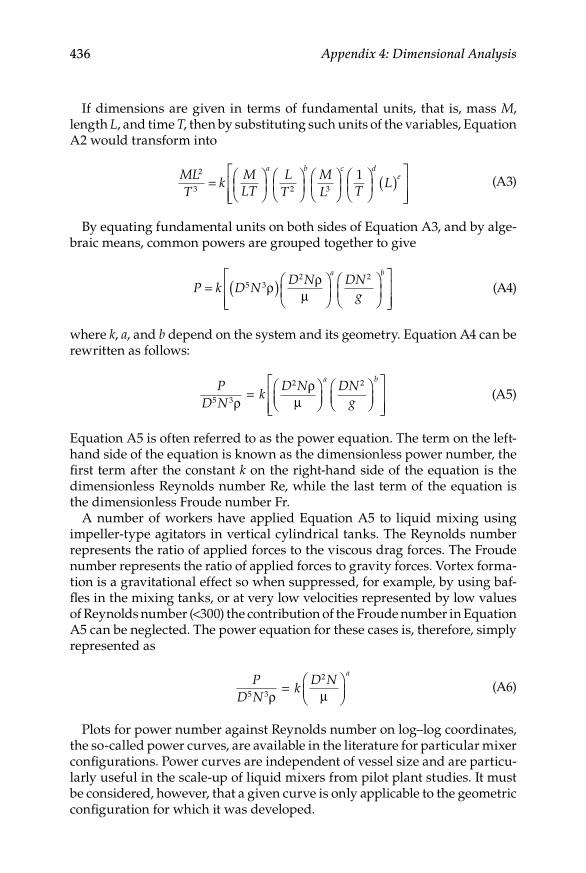
436 Appendix 4: Dimensional Analysis
If dimensions are given in terms of fundamental units, that is, mass M, length L, and time T, then by substituting such units of the variables, Equation A2 would transform into
MLT
kMLT
LT
ML T
La b c d
e2
3 2 3=
( )
1
(A3)
By equating fundamental units on both sides of Equation A3, and by alge-braic means, common powers are grouped together to give
P k D ND N DN
g
a b
= ( )
5 32 2
ρ ρµ
(A4)
where k, a, and b depend on the system and its geometry. Equation A4 can be rewritten as follows:
PD N
kD N DN
g
a b
5 3
2 2
ρρ
µ=
(A5)
Equation A5 is often referred to as the power equation. The term on the left-hand side of the equation is known as the dimensionless power number, the first term after the constant k on the right-hand side of the equation is the dimensionless Reynolds number Re, while the last term of the equation is the dimensionless Froude number Fr.
A number of workers have applied Equation A5 to liquid mixing using impeller-type agitators in vertical cylindrical tanks. The Reynolds number represents the ratio of applied forces to the viscous drag forces. The Froude number represents the ratio of applied forces to gravity forces. Vortex forma-tion is a gravitational effect so when suppressed, for example, by using baf-fles in the mixing tanks, or at very low velocities represented by low values of Reynolds number (<300) the contribution of the Froude number in Equation A5 can be neglected. The power equation for these cases is, therefore, simply represented as
PD N
kD N
a
5 3
2
ρ µ=
(A6)
Plots for power number against Reynolds number on log–log coordinates, the so-called power curves, are available in the literature for particular mixer configurations. Power curves are independent of vessel size and are particu-larly useful in the scale-up of liquid mixers from pilot plant studies. It must be considered, however, that a given curve is only applicable to the geometric configuration for which it was developed.
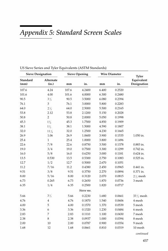
437
Appendix 5: Standard Screen Scales
US Sieve Series and Tyler Equivalents (ASTM Standards)
Sieve Designation Sieve Opening Wire DiameterTyler
Equivalent Designation
Standard (mm)
Alternate (in.) mm in. mm in.
107.6 4.24 107.6 4.2400 6.400 0.2520101.6 4.00 101.6 4.0000 6.300 0.248090.5 3 1
2 90.5 3.5000 6.080 0.2394
76.1 3 76.1 3.0000 5.800 0.228364.0 2 1
2 64.0 2.5000 5.500 0.216553.8 2.12 53.8 2.1200 5.150 0.202850.8 2 50.8 2.0000 5.050 0.199845.3 13
4 45.3 1.7500 4.850 0.190938.1 1 1
2 38.1 1.5000 4.590 0.180732.0 11 1
4 32.0 1.2500 4.230 0.166526.9 1.06 26.9 1.0600 3.900 0.1535 1.050 in.25.4 1 25.4 1.0000 3.800 0.149622.6 7/8 22.6 0.8750 3.500 0.1378 0.883 in.19.0 3/4 19.0 0.7500 3.300 0.1299 0.742 in.16.0 5/8 16.0 0.6250 3.000 0.1181 0.624 in.13.5 0.530 13.5 0.5300 2.750 0.1083 0.525 in.12.7 1/2 12.7 0.5000 2.670 0.105111.2 7/16 11.2 0.4380 2.450 0.0965 0.441 in.9.51 3/8 9.51 0.3750 2.270 0.0894 0.371 in.8.00 5/16 8.00 0.3120 2.070 0.0815 2 1
2 mesh6.73 0.265 6.73 0.2650 1.870 0.0736 3 mesh6.35 1/4 6.35 0.2500 1.820 0.0717
Sieve no.
5.66 3 12 5.66 0.2230 1.680 0.0661 33 1
2 mesh
4.76 4 4.76 0.1870 1.540 0.0606 4 mesh4.00 5 4.00 0.1570 1.370 0.0539 5 mesh3.36 6 3.36 0.1320 1.230 0.0484 6 mesh2.83 7 2.83 0.1110 1.100 0.0430 7 mesh2.38 8 2.38 0.0937 1.000 0.0394 8 mesh2.00 10 2.00 0.0787 0.900 0.0354 9 mesh1.68 12 1.68 0.0661 0.810 0.0319 10 mesh
continued

438 Appendix 5: Standard Screen Scales
British Standard Sieves
Nominal Aperture Size (mm)
Nominal Wire Diameter (mm)
Nearest Mesh Number
16.0 3.1513.2 2.8011.2 2.509.50 2.248.00 2.006.70 1.805.60 1.60 34.75 1.60 3 1
2
4.00 1.40 4
(continued)
US Sieve Series and Tyler Equivalents (ASTM Standards)
Sieve Designation Sieve Opening Wire DiameterTyler
Equivalent Designation
Standard (mm)
Alternate (in.) mm in. mm in.
1.41 14 1.41 0.0555 0.725 0.0285 12 mesh1.19 16 1.19 0.0469 0.650 0.0256 14 mesh1.00 18 1.00 0.0394 0.580 0.0228 16 mesh
Micrometers841 20 0.841 0.0331 0.510 0.0201 20 mesh707 25 0.707 0.0278 0.450 0.0177 24 mesh595 30 0.595 0.0234 0.390 0.0154 28 mesh500 35 0.500 0.0197 0.340 0.0134 32 mesh420 40 0.420 0.0165 0.290 0.0114 35 mesh354 45 0.354 0.0139 0.247 0.0097 42 mesh297 50 0.297 0.0117 0.215 0.0085 48 mesh250 60 0.250 0.0098 0.180 0.0071 60 mesh210 70 0.210 0.0083 0.152 0.0060 65 mesh177 80 0.177 0.0070 0.131 0.0052 80 mesh149 100 0.149 0.0059 0.110 0.0043 100 mesh125 120 0.125 0.0049 0.091 0.0036 115 mesh105 140 0.105 0.0041 0.076 0.0030 150 mesh88 170 0.088 0.0035 0.064 0.0025 170 mesh74 200 0.074 0.0029 0.053 0.0021 200 mesh63 230 0.063 0.0025 0.044 0.0017 250 mesh53 270 0.053 0.0021 0.037 0.0015 270 mesh44 325 0.044 0.0017 0.030 0.0012 325 mesh37 400 0.037 0.0015 0.025 0.0010 400 mesh
continued

Appendix 5: Standard Screen Scales 439
(continued)
British Standard Sieves
Nominal Aperture Size (mm)
Nominal Wire Diameter (mm)
Nearest Mesh Number
3.35 1.25 52.80 1.12 62.36 1.00 72.00 0.90 81.70 0.80 101.40 0.71 121.18 0.63 141.00 0.56 16
Micrometers
850 500 18710 450 22600 400 25500 315 30425 280 36355 224 44300 200 52250 160 60212 140 72180 125 85150 100 100125 90 120106 71 15090 63 17075 50 20063 45 24053 36 30045 32 35038 30 400


441
Appendix 6: Guidelines for the Preparation of Laboratory Reports
The most common means of technical communication within and among organizations of all sorts, including industry, educational institutions, and professional societies, is the written technical report or article. In any profes-sional activity, the writing and submission of reports is most certainly required. The technical report gives an insight into the writer’s competences, abilities, and skills. It also reflects the writer’s work habits and productivity. Regardless of the quality of the work reported, a poorly written report will reflect unfavorably on the writer.
Introductory Aspects
It is impossible to describe a standard format for the organization and con-tents of a given report. High-quality well-written reports contain, however, the following common components:
Clearness of development•
Conciseness of expression•
Completeness of information•
Accuracy of details•
Correctness of form•
Convenience of layout•
The details of format and content should be selected in full consideration of the reader’s point of view and the purpose of the report. This criterion generally applies to classroom reports, as well as those expected to be produced after graduation in all types of arenas and scenarios.

442 Appendix 6: Guidelines for the Preparation of Laboratory Reports
The Importance of Neatness
From the days when typewriters were used, or even handwriting, the key characteristic of a written report has been its neatness and readability. In earlier days, decisions had to be made on whether to correct or amend parts of a document in the best possible way without sacrificing neatness, or rewrite a whole page or part. Nowadays, the ease of resourcing to the famous “copy–paste” practice, and some other similar alternatives, has created a trend to abuse of such routines so as to present bulky and appar-ently complete reports. Regardless of the audience to whom the document is written, reports are to be read by panels of experts in their fields of interest. Direct copy–paste inserts and some other editorial anomalies, in content as well as in format, will be detected by the trained eye. It is advisable to prepare figures and inserts with the text processor being used in writing, as well as to give uniformity of style to imported ideas from other texts.
Use of the English Language
The triumph of the Allies in World War II, along with a series of social and cultural events mainly in the twentieth century, has made English the undis-putable recognized international language. Thus, writing skills in English are paramount since business, culture, and among all, science interchange, are made based on English written reports, articles, books, media presenta-tions, and so on. Students in higher education programs all over the world may need to write technical reports in their own language, but after gradua-ting, the importance of acquiring abilities to write in English increases sig-nificantly in order to gain access to more opportunities for professional development.
In technical and scientific reports it is good practice to use short, precise sentences and make sure that the text is written in sentences and not in phrases. Principles for punctuation and abbreviations should be used at all times. It is important to pay particular attention to spelling, sentence struc-ture, agreement between subject and verb, and the use of consistent tense. It is also relevant to make sure that misinterpretation and unintended meanings are minimized. Once completed, the report is to be read thoroughly several times for assessing content and organization, as well as to perform a proof-reading. It is advisable to ask a classmate to read and criticize the report. Even the most professional authors usually have to rewrite parts of a written document.

Appendix 6: Guidelines for the Preparation of Laboratory Reports 443
Report Organization and Content
Title Page
The title page should be the first page of a formal report. The title should state briefly and completely the subject of the report. The name or organization or person for whom the report was prepared, the name of the individual or organization submitting the report, and the date should appear on the title page. Short or informal reports do not require a separate title page. In this instance, the title, the name of the writer, and the organization recipient of the report, should appear on the first page together with the abstract.
Table of Contents
Lengthy and formal reports require a table of contents, while short and infor-mal reports do not. Most of the reports to be written by students will fall some-where between these two extremes and, thus, the decision on whether or not to include a table of contents will be a matter of judgment. Whenever a table of contents will significantly clarify and demonstrate the continuity of the report, help the reader understanding the scope, or make it more convenient for the reader to find any point of interest, such a table should be included.
A table of contents should list, by title and page number, the divisions and subdivisions of the report in the order they appear, including all appendices. Tables and figures should be identified by number, title, and page in separate lists immediately following the table of contents. Page numbers, titles, and all the components of each item shown in the table of contents should be double-checked in a proofreading against the title, page, and so on, where the item occurs in the report.
abstract
This section of the report is the most important individual section. The objec-tive of the abstract is to provide the reader with a concise, overall statement of the high points of the report. Normally, the abstract should be no more than one written page. More than any other section of the report, the abstract should be prepared in consideration of the reader and the purpose of the own report. A reasonable assessment of the abstract will be, therefore, to read it from the reader’s point of view and determine if is sufficiently clear and concise and conveys the appropriate information on the purpose, scope, and extent of the report. A good abstract will include a brief statement of the objectives of the study, experiment, or design, and results in the form on concise conclusions and/or recommendations for further work. Often, other information, such as important assumptions, alternatives analyzed, or procedures will be included depending on the purpose of the report and the reader’s profile.

444 Appendix 6: Guidelines for the Preparation of Laboratory Reports
introduction
The purpose of the introduction is to give the reader the minimum amount of information needed to understand the result, conclusions, and recommen-dations. Such information normally includes purpose (problem statement), scope, and nature of the study. A formal introduction may not be required for short reports where minimal background is required for understanding. A simple introductory statement will be sufficient in cases such as this.
objectives
This section of the report should itemize in a brief, but clear manner, all the objectives of the work performed. No detailed description of each objective is required at this point and the best format is probably a simple listing of line items.
background
The contents of this section, depends upon the nature of the work being reported. In general, theoretical principles related to the subject under study are to be explained and briefly discussed. A literature survey, as current as possible but balanced with classical references if appropriate, is a funda-mental part of this section. Any derivations and equations used in the devel-opment of the work reported should be included in this part of the report. If alternate approaches were performed, a justification should be also given in this section. Assumptions made in the development of the work, should be stated and sufficiently supported.
Materials and Methods
A description of the equipment, instruments, and apparatuses used to per-form the work should be included in this section. Raw materials used, rou-tine procedures employed, and glassware along with consumables utilized, may be simply listed. Quite often, neat schematic diagrams of equipment and instruments will greatly enhance the clarity of the written text. The experimental methods should be clearly described, with reference given to standard methods like those reported in analytical chemists handbooks. The aim is for the reader to understand fully how the raw data were collected.
results and interpretation of Data
The result obtained from the work should be presented in this section. It is important to point out that these results are not the raw data collected from the methods described in the previous section, but the final values resulting from the computational analysis based on the raw data collected. When

Appendix 6: Guidelines for the Preparation of Laboratory Reports 445
possible, the results should be presented in tabular or graphical form. Table and/or figures cannot constitute, however, this section on their own. Some explanatory text must be incorporated to lead the reader through the results. Whenever possible, a statistical analysis on the data collected should be performed and the results included in this section.
Discussion
This section of the reports should include a critical analysis of the results obtained. It is appropriate at this stage to discuss items such as accuracy of the data, limitations imposed by the assumptions, comparisons with results available in the literature, operating problems due to availability of equip-ment, instruments, and infrastructure, and so on. Compatible comparisons with results in the literature are important in this section, so that few or several references will be appropriate.
Conclusions
The logical deduction of conclusions from the results should be clearly demonstrated. An itemization of conclusions from the work performed may be an appropriate format for this section.
recommendations
A list of specific suggestions on how to improve the quality of the work reported is appropriate after the section of conclusions. These recommendations should address items such as experimental design, equipment modifications, sample collection systems, need for further work, and so on. Conclusions and Recommendations may conform into a single section.
references, literature Cited
Use of cited references is an important part of a technical report. Cited litera-ture is a basic foundation for the reader to realize that the report makes sense within the state-of-the-art of the related discipline. For this reason, normally all the literature is cited in a technical report and, as such, the proper denominations should be References or Literature Cited. Bibliography is usually not an appropriate title for this section. Some textbooks and encyclo-pedias often refer to suggested readings or bibliography, that have not been cited in the text, for the reader to get further information on some topics discussed. In this section, each reference cited in the body of the report should be listed in detail, so that an interested reader can find the article, book, or report. There are several references styles used in scientific litera-ture, such as the American Chemical Society style or the Harvard style. As long as the references listed are consistent, any scientific style can be used.

446 Appendix 6: Guidelines for the Preparation of Laboratory Reports
appendices
The body of the report should contain only those data, equations, drawings, or calculations, which pertain directly to results of the work. This informa-tion is often the result of much detailed data, computations, derivations, and so on, and it is usually desirable to place the latter in appendices to the main report. Specific examples of information that should be placed in appendices are raw data from experiments, detailed derivation of an equation, example computations, statistical tables of data interpretation such as analyses of variance, and so on. It is good practice to include sufficiently detailed infor-mation in appendices to allow the reader to check computations or conclu-sions of the report.
illustrative aids
Tables, charts, graphs, drawings, and photographs are valuable aids for presenting technical information and should be considered an integral part of the report. As such, they must be planned and prepared in rough form as the text itself is planned and developed. Illustrative aids, while based on the text, should be as nearly self-explanatory as possible, and reliance upon the text for clarification of illustrations should be kept to a minimum. Every illustration should be accompanied by a caption, which makes clear the nature of the contents and the meaning or significance of the information. Tables and figures should be identified by number and title. Reference to a particular table or figure in the text should be properly accomplished as, for example: Table 4 or Figure 5.
Tables
Tables should be prepared so that the arrangement maximizes clarity. Only relevant data should be included. Titles should be clear and complete, and placed at the top of the tables. It is permissible to use footnotes, which apply to specific portions of the table, immediately below it. Column headings should clearly identify the data in the column and include units in which the numbers are expressed. Columns and rows should be placed to facilitate ease of reading.
Drawings and Diagrams
It is important to make sure that all drawings and diagrams have a figure number and an appropriate caption or title. All pertinent parts of these figures should be clearly labeled and dimensioned. Overcrowding of draw-ings is to be avoided, so neatness and readability are satisfactory. As stated earlier, crude paste of imported figures is noticeable, while it demerits the quality of the report. It is preferable to make use of the available tool for

Appendix 6: Guidelines for the Preparation of Laboratory Reports 447
graphics in the word processor, or to insert figures prepared in a compatible graphics elaboration system.
Charts and graphs
Data, numerical results, and some other information should be presented in charts and graphs when possible. This type of presentation is usually superior to a tabular presentation because trends, comparisons, and relationships are more easily identified. Charts and graphs should be presented on a grid. The scale of the ordinate and the abscissa should be clear. It is recommended practice to measure the independent variable on the abscissa and the depen-dent variable on the ordinate. Both axes should be clearly labeled with the variable name, symbol, and units. If more than one curve is plotted, the con-ditions for each one should be identified. It is usually best to use different symbols and/or different types of lines for different curves. Colored lines or markers are not recommended because of problems in reproduction of reports. It is advisable to plot measured data at discrete points and reserve the use of continuous curves for theoretical or best-fit relations. Bar graphs are very useful in presenting data for which the relationship between variables is discontinuous.
equations
Formulas and equations are often a very important component of a technical report. It is essential that all variables, exponents, parameter, and so on, be clearly defined immediately following the equation. The units of each com-ponent of an equation should be stated. Use of SI units is preferred. If the formula is written so that it is valid for any consistent set of units, then the fundamental dimension, for example, length or force, of each symbol should be listed. For lengthy reports including many equations, a list of nomencla-ture placed normally right after the list of tables and figures or right before the references, is recommended.

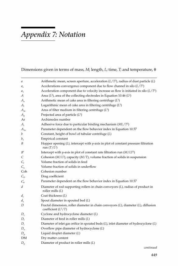
449
Appendix 7: Notation
Dimensions given in terms of mass, M; length, L; time, T; and temperature, θ
a Arithmetic mean, screen aperture, acceleration (L/T2), radius of dust particle (L)ac Accelerations convergence component due to flow channel in silo (L/T2)av Acceleration component due to velocity increase as flow is initiated in silo (L/T2)A Area (L2), area of the collecting electrodes in Equation 10.46 (L2)Aa Arithmetic mean of cake area in filtering centrifuge (L2)Al Logarithmic mean of cake area in filtering centrifuge (L2)Am Area of filter medium in filtering centrifuge (L2)Ap Projected area of particle (L2)Ar Archimedes numberAi Adhesive force due to particular binding mechanism (ML/T2)A1n Parameter dependent on the flow behavior index in Equation 10.57b Constant, height of bowl of tubular centrifuge (L)b1 Empirical constantB Hopper opening (L), intercept with y-axis in plot of constant pressure filtration
run (T/L3)B′ Intercept with y-axis in plot of constant rate filtration run (M/LT2)C Cohesion (M/L2), capacity (M/T), volume fraction of solids in suspensionCf Volume fraction of solids in feedCu Volume fraction of solids in underflowCoh Cohesion numberCD Drag coefficient
Cn' Parameter dependent on the flow behavior index in Equation 10.57
d Diameter of rod supporting rollers in chain conveyors (L), radius of product in roller mills (L)
dc Coat thickness (L)ds Spout diameter in spouted bed (L)D Fractal dimension, roller diameter in chain conveyors (L), diameter (L), diffusion
coefficient (L2/T)Dc Cyclone and hydrocyclone diameter (L)Df Diameter of feed in roller mills (L)Di Diameter of inlet gas orifice in spouted beds (L), inlet diameter of hydrocyclone (L)Do Overflow pipe diameter of hydrocyclone (L)Dp Liquid droplet diameter (L)DM Dry matter contentDp Diameter of product in roller mills (L)
continued

450 Appendix 7: Notation
(continued)
Dpc Cut diameter (L)Dr Diameter of roll in roller mills (L)Dt Pipe diameter (L)Du Underflow diameter of hydrocyclone (L)E Energy (ML2/T2), overall screen efficiencyEa Acceptance efficiencyEc Coating efficiencyEfb Friction energy due to flow round bends expressed as pressure drop in
pneumatic conveying (M/LT2)Efg Friction energy due to gas flow expressed as pressure drop in pneumatic
conveying (M/LT2)Efp Friction energy due to particle flow expressed as pressure drop in pneumatic
conveying (M/LT2)Ef Net efficiency of finesEi Bond work index (ML2/T2)Ek Kinetic energy expressed as pressure drop in pneumatic conveying (M/LT2)EO Oversize screen efficiencyEp Potential energy expressed as pressure drop in pneumatic conveying (M/LT2),
partial efficiency, strength of electrical field in settling point (Va/T)Er Rejection efficiencyEs Screen efficiencyEt Total efficiency
Et' Reduced total efficiency
Eu Euler numberEU Undersize screen efficiencyE0 Strength of electrical field (Va/L)f Frequency (dimensionless) frequency (1/T), fanning friction factor, ratio of
filtration to cycle time in Equation 10.125fa Size fraction of one component of average weight wa
fb Bend friction factorfg Gas friction factorfp Particle friction factorff Flow factorffa Actual flow factor based on the actual opening dimensionfam(x) Modified beta distribution given by Equation 2.27fpv Purely viscous fanning friction factorf(x) Frequency or occurrence related to sizefL(x) Size distribution function by lengthfM(x) Size distribution function by mass (volume)fN(x) Size distribution function by numberfS(x) Size distribution function by surfacef(δ) Constant related to angle of contact of particles in agglomeratesF Mass flow rate of solids in feed (M/T), force (ML/T2), cumulative percentage of
coarse fraction in the feed
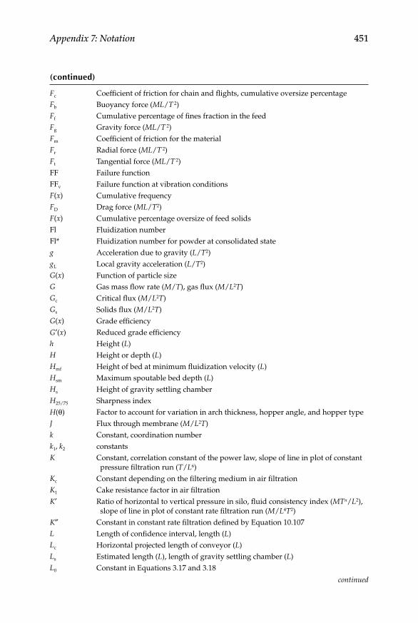
Appendix 7: Notation 451
(continued)
Fc Coefficient of friction for chain and flights, cumulative oversize percentageFb Buoyancy force (ML/T 2)Ff Cumulative percentage of fines fraction in the feedFg Gravity force (ML/T 2)Fm Coefficient of friction for the materialFr Radial force (ML/T 2)Ft Tangential force (ML/T 2)FF Failure functionFFv Failure function at vibration conditionsF(x) Cumulative frequencyFD Drag force (ML/T2)F(x) Cumulative percentage oversize of feed solidsFl Fluidization numberFl* Fluidization number for powder at consolidated stateg Acceleration due to gravity (L/T2)gL Local gravity acceleration (L/T2)G(x) Function of particle sizeG Gas mass flow rate (M/T), gas flux (M/L2T)Gc Critical flux (M/L2T)Gs Solids flux (M/L2T)G(x) Grade efficiencyG′(x) Reduced grade efficiencyh Height (L)H Height or depth (L)Hmf Height of bed at minimum fluidization velocity (L)Hsm Maximum spoutable bed depth (L)Hs Height of gravity settling chamberH25/75 Sharpness indexH(θ) Factor to account for variation in arch thickness, hopper angle, and hopper typeJ Flux through membrane (M/L2T)k Constant, coordination numberk1, k2 constantsK Constant, correlation constant of the power law, slope of line in plot of constant
pressure filtration run (T/L6)Kc Constant depending on the filtering medium in air filtrationK1 Cake resistance factor in air filtrationK′ Ratio of horizontal to vertical pressure in silo, fluid consistency index (MTn/L2),
slope of line in plot of constant rate filtration run (M/L4T2)K″ Constant in constant rate filtration defined by Equation 10.107L Length of confidence interval, length (L)Lc Horizontal projected length of conveyor (L)Ls Estimated length (L), length of gravity settling chamber (L)L0 Constant in Equations 3.17 and 3.18
continued
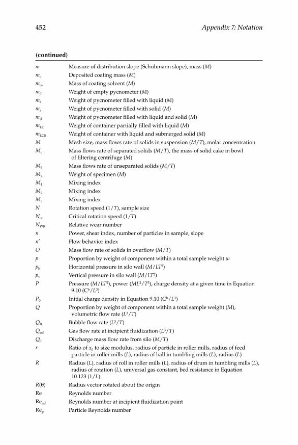
452 Appendix 7: Notation
(continued)
m Measure of distribution slope (Schuhmann slope), mass (M)
mc Deposited coating mass (M)
mcs Mass of coating solvent (M)
m0 Weight of empty pycnometer (M)
ml Weight of pycnometer filled with liquid (M)
ms Weight of pycnometer filled with solid (M)
msl Weight of pycnometer filled with liquid and solid (M)
mLC Weight of container partially filled with liquid (M)
mLCS Weight of container with liquid and submerged solid (M)
M Mesh size, mass flows rate of solids in suspension (M/T), molar concentration
Mc Mass flows rate of separated solids (M/T), the mass of solid cake in bowl of filtering centrifuge (M)
Mf Mass flows rate of unseparated solids (M/T)
Ms Weight of specimen (M)
M1 Mixing index
M2 Mixing index
M3 Mixing index
N Rotation speed (1/T), sample size
Ncr Critical rotation speed (1/T)
NWR Relative wear number
n Power, shear index, number of particles in sample, slope
n′ Flow behavior index
O Mass flow rate of solids in overflow (M/T)
p Proportion by weight of component within a total sample weight w
ph Horizontal pressure in silo wall (M/LT2)
pv Vertical pressure in silo wall (M/LT2)
P Pressure (M/LT2), power (ML2/T3), charge density at a given time in Equation 9.10 (Cb/L3)
P0 Initial charge density in Equation 9.10 (Cb/L3)
Q Proportion by weight of component within a total sample weight (M), volumetric flow rate (L3/T)
QB Bubble flow rate (L3/T)
Qmf Gas flow rate at incipient fluidization (L3/T)
Q0 Discharge mass flow rate from silo (M/T)
r Ratio of x0 to size modulus, radius of particle in roller mills, radius of feed particle in roller mills (L), radius of ball in tumbling mills (L), radius (L)
R Radius (L), radius of roll in roller mills (L), radius of drum in tumbling mills (L), radius of rotation (L), universal gas constant, bed resistance in Equation 10.123 (1/L)
R(θ) Radius vector rotated about the origin
Re Reynolds number
Remf Reynolds number at incipient fluidization point
Rep Particle Reynolds number
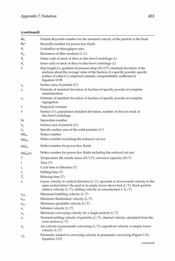
Appendix 7: Notation 453
(continued)
Ret Particle Reynolds number for the terminal velocity of the particle in the fluidRe* Reynolds number for power-law fluidsRf Underflow-to-throughput ratioRm Resistance of filter medium (1/L)Rx Outer radii of stack of discs in disc-bowl centrifuge (L)Ry Inner radii of stack of discs in disc-bowl centrifuge (L)S Step length (L), gradient of pressure drop (M/LT2), standard deviation of the
analyses about the average value of the fraction of a specific powder, specific surface of solid (L2), empirical constant, compressibility coefficient in Equation 10.98
sp Surface area of particle (L2)sr Estimate of standard deviation of fraction of specific powder at complete
randomizations0 Estimate of standard deviation of fraction of specific powder at complete
segregations′ Empirical constantS Surface (L2), population standard deviation, number of discs in stack in
disc-bowl centrifugeSe Separation numberSp Surface area of particle (L2)S0 Specific surface area of the solid particles (L2)Stk50 Stokes number
Stk50′ Stokes number including the reduced cut size
Stk50* Stokes number for power-law fluids
Stk50* (r) Stokes number for power-law fluids including the reduced cut size
T Temperature (θ), tensile stress (M/LT2), conveyor capacity (M/T)t Time (T)tc Cycle time in filtration (T)ts Settling time (T)Tr Relaxing time (T)u Linear velocity in vertical direction (L/T), upwards or downwards velocity in the
open section below the grid or in empty tower above bed (L/T), fluid–particle relative velocity (L/T), settling velocity at concentration C (L/T)
umb Minimum bubbling velocity (L/T)umf Minimum fluidization velocity (L/T)ums Minimum spoutable velocity (L/T)us Saltation velocity (L/T)uss Minimum conveying velocity for a single particle (L/T)ut Terminal settling velocity of particles (L/T), channel velocity calculated from the
cross section (L/T)u0 Air velocity in pneumatic conveying (L/T), superficial velocity or empty-tower
velocity (L/T)
uss∗ Parameter related to conveying velocity in pneumatic conveying (Figure 3.33,
Equation 3.27)continued
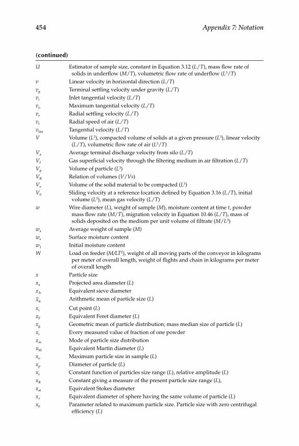
454 Appendix 7: Notation
(continued)
U Estimator of sample size, constant in Equation 3.12 (L/T), mass flow rate of solids in underflow (M/T), volumetric flow rate of underflow (L3/T)
v Linear velocity in horizontal direction (L/T)vg Terminal settling velocity under gravity (L/T)vi Inlet tangential velocity (L/T)vo Maximum tangential velocity (L/T)vr Radial settling velocity (L/T)vt Radial speed of air (L/T)vtan Tangential velocity (L/T)V Volume (L3), compacted volume of solids at a given pressure (L3), linear velocity
(L/T), volumetric flow rate of air (L3/T)Va Average terminal discharge velocity from silo (L/T)Vf Gas superficial velocity through the filtering medium in air filtration (L/T)Vp Volume of particle (L3)VR Relation of volumes (V/Vs)Vs Volume of the solid material to be compacted (L3)V0 Sliding velocity at a reference location defined by Equation 3.16 (L/T), initial
volume (L3), mean gas velocity (L/T)w Wire diameter (L), weight of sample (M), moisture content at time t, powder
mass flow rate (M/T), migration velocity in Equation 10.46 (L/T), mass of solids deposited on the medium per unit volume of filtrate (M/L3)
wa Average weight of sample (M)ws Surface moisture contentw1 Initial moisture contentW Load on feeder (M/LT2), weight of all moving parts of the conveyor in kilograms
per meter of overall length, weight of flights and chain in kilograms per meter of overall length
x Particle sizexa Projected area diameter (L)xA Equivalent sieve diameter
xa Arithmetic mean of particle size (L)
xc Cut point (L)xF Equivalent Feret diameter (L)xg Geometric mean of particle distribution; mass median size of particle (L)xi Every measured value of fraction of one powderxm Mode of particle size distributionxM Equivalent Martin diameter (L)xo Maximum particle size in sample (L)xp Diameter of particle (L)xr Constant function of particles size range (L), relative amplitude (L)xR Constant giving a measure of the present particle size range (L),xst Equivalent Stokes diameterxv Equivalent diameter of sphere having the same volume of particle (L)x0 Parameter related to maximum particle size. Particle size with zero centrifugal
efficiency (L)

Appendix 7: Notation 455
(continued)
x50 Cut size (L)x98 Approximate particle size fully separated (L)
xp∗ Parameter related to particle size in pneumatic conveying (Equation 3.26)
x50′ Reduced cut size (L)
X FractionXF Mass fraction of coarse particles in feedXi Assayed valueXO Mass fraction of coarse particles in the overflowXr Value of particular amplitude defined in Equation 3.13 (L)XU Mass fraction of coarse particles in the underflow
X Sample arithmetic average
y Probability densityY Cumulative weight fraction undersize, solids yield in Equation 10.125 (M/L2T)Z(1–α)/2 (1–α)/2 percentile of standard Normal variable
Greek letters
α Angle of repose, half the angle of nip in roller mills, surface tension of liquid (M/LT2), degree of separation, specific cake resistance (L/M)
αs Surface factor defined in Equation 1.3
αv Volume factor defined in Equation 1.2
α0 Empirical constant in Equation 10.98α0
′ Empirical constant in Equation 10.99β Empirical constant in Equation 10.99
β′ Parameter in Equation 3.50
γ Viscosity coefficient for power-law fluids (M/LT2–n)
γn Volume reduction fraction
γ Shear rate (1/T)
δ Effective angle of internal friction, membrane thickness (L)
ΔP Pressure drop (M/LT2), pressure drop across fixed bed (M/LT2)
ΔPB Pressure drop across fluidized bed (M/LT2)
ΔPc Pressure drop through powder layer in air filtration (M/LT2)
ΔPeq Pressure drop equal to buoyant weight of particles per unit area of bed (M/LT2)
ΔPf Pressure drop across the filtering medium of air filter (M/LT2)
ΔPSB Total spouting pressure drop at maximum spoutable bed depth (M/LT2)
–ΔP Total pressure drop across the filter (M/LT2)
–ΔPc Pressure drops across the cake (M/LT2)
–ΔPm Pressure drops across the medium (M/LT2)
ε Porosity or voidage, permeability in Equation 9.10
εB Fraction of bed occupied by bubbles
εmf Voidage of bed at minimum fluidization velocity
η Efficiency of separation in gravity settling chamber
θ Hopper half-angle, hydrocyclone cone angle
continued
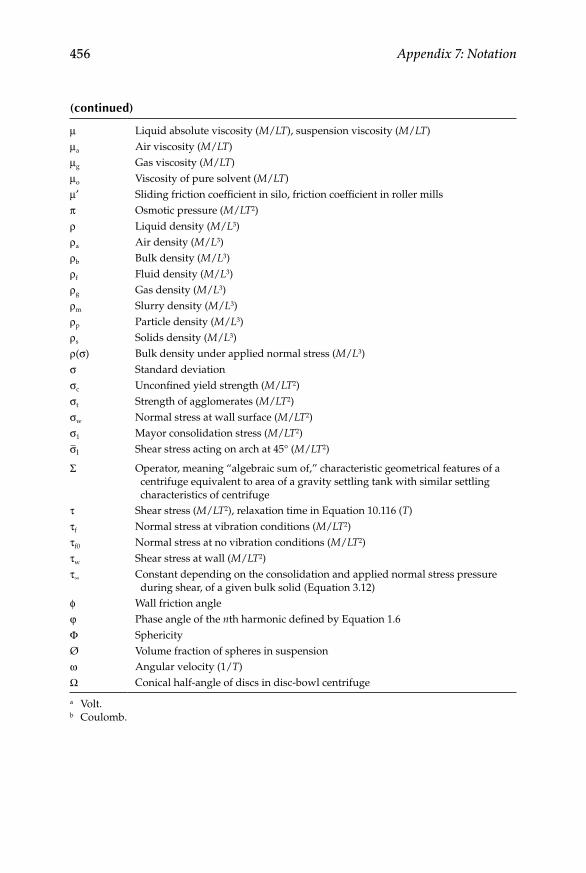
456 Appendix 7: Notation
(continued)
μ Liquid absolute viscosity (M/LT), suspension viscosity (M/LT)
μa Air viscosity (M/LT)
μg Gas viscosity (M/LT)
μo Viscosity of pure solvent (M/LT)
μ′ Sliding friction coefficient in silo, friction coefficient in roller mills
π Osmotic pressure (M/LT2)
ρ Liquid density (M/L3)
ρa Air density (M/L3)
ρb Bulk density (M/L3)
ρf Fluid density (M/L3)
ρg Gas density (M/L3)
ρm Slurry density (M/L3)
ρp Particle density (M/L3)
ρs Solids density (M/L3)
ρ(σ) Bulk density under applied normal stress (M/L3)
σ Standard deviation
σc Unconfined yield strength (M/LT2)
σt Strength of agglomerates (M/LT2)
σw Normal stress at wall surface (M/LT2)
σ1 Mayor consolidation stress (M/LT2)
σ1 Shear stress acting on arch at 45° (M/LT2)
Σ Operator, meaning “algebraic sum of,” characteristic geometrical features of a centrifuge equivalent to area of a gravity settling tank with similar settling characteristics of centrifuge
τ Shear stress (M/LT2), relaxation time in Equation 10.116 (T)
τf Normal stress at vibration conditions (M/LT2)
τf0 Normal stress at no vibration conditions (M/LT2)
τw Shear stress at wall (M/LT2)
τ∞ Constant depending on the consolidation and applied normal stress pressure during shear, of a given bulk solid (Equation 3.12)
ϕ Wall friction angle
φ Phase angle of the nth harmonic defined by Equation 1.6
Φ SphericityØ Volume fraction of spheres in suspensionω Angular velocity (1/T)
Ω Conical half-angle of discs in disc-bowl centrifuge
a Volt.b Coulomb.
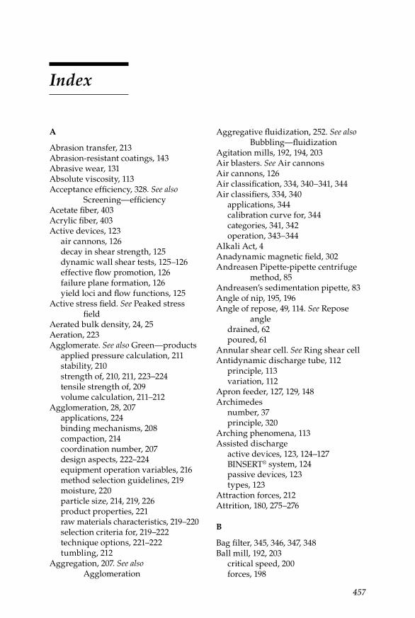
457
A
Abrasion transfer, 213Abrasion-resistant coatings, 143Abrasive wear, 131Absolute viscosity, 113Acceptance efficiency, 328. See also
Screening—efficiencyAcetate fiber, 403Acrylic fiber, 403Active devices, 123
air cannons, 126decay in shear strength, 125dynamic wall shear tests, 125–126effective flow promotion, 126failure plane formation, 126yield loci and flow functions, 125
Active stress field. See Peaked stress field
Aerated bulk density, 24, 25Aeration, 223Agglomerate. See also Green—products
applied pressure calculation, 211stability, 210strength of, 210, 211, 223–224tensile strength of, 209volume calculation, 211–212
Agglomeration, 28, 207applications, 224binding mechanisms, 208compaction, 214coordination number, 207design aspects, 222–224equipment operation variables, 216method selection guidelines, 219moisture, 220particle size, 214, 219, 226product properties, 221raw materials characteristics, 219–220selection criteria for, 219–222technique options, 221–222tumbling, 212
Aggregation, 207. See also Agglomeration
Aggregative fluidization, 252. See also Bubbling—fluidization
Agitation mills, 192, 194, 203Air blasters. See Air cannonsAir cannons, 126Air classification, 334, 340–341, 344Air classifiers, 334, 340
applications, 344calibration curve for, 344categories, 341, 342operation, 343–344
Alkali Act, 4Anadynamic magnetic field, 302Andreasen Pipette-pipette centrifuge
method, 85Andreasen’s sedimentation pipette, 83Angle of nip, 195, 196Angle of repose, 49, 114. See Repose
angledrained, 62poured, 61
Annular shear cell. See Ring shear cellAntidynamic discharge tube, 112
principle, 113variation, 112
Apron feeder, 127, 129, 148Archimedes
number, 37principle, 320
Arching phenomena, 113Assisted discharge
active devices, 123, 124–127BINSERT® system, 124passive devices, 123types, 123
Attraction forces, 212Attrition, 180, 275–276
B
Bag filter, 345, 346, 347, 348Ball mill, 192, 203
critical speed, 200forces, 198
Index

458 Index
Bar screens. See GrizzliesBasket
centrifuge, 390extruder, 216
Belt, 137conveyor, 136, 138, 142separator, 303thickness, 142
Belt conveyors, 136characteristics of solid, 142–143components, 136, 137idler, 138–139power for, 140–142, 143pulley transmission relations, 142tension devices, 138, 139thickness of, 142tripper, 139–140
Belt feeder. See Apron feederBinder, 212, 220, 225. See also WaterBingham plastic fluids, 318, 319Bins, 102. See also Hopper; Silos
design considerations, 103funnel flow, 104–107mass-flow, 104stress fields, 108–109wall load prediction, 108
Binsert® system, 123, 124. See also Passive devices
Blake crushers, 185, 186Blending
indices determination, 244–245mechanism, 230–231quality, 229, 233uniformity, 242
Bond Work Index, 184Bond’s law, 184Breakage stages, 182Bridging phenomena. See Arching
phenomenaBriquetting roller press, 217British standard sieves, 438–439Bubble, 249, 252
air, 20behavior, 262in gas-fluidized bed, 261powder effect, 34in solid–gas systems, 262
Bubblingfluidization, 261
phase, 262in solid–gas systems, 262
Bubbling fluidized bedbubbling phase, 262particulate phase, 262, 263
Bucket elevators, 148, 149buckets, 149horsepower, 150–151spacing of buckets, 19–150
Bulk, 24density, 23, 24, 250
Bulk solid, 31failure properties, 48, 65flow types, 104handling plants, 104, 131, 132particle size analysis, 67, 89powder classification, 32sampling, 37
Bulk solid, storage, 101confined storage, 102outdoors storage, 101storage alternatives, 101wall loads in silos evaluation, 134
Bulk solid conveying, 135belt conveyors, 136–143capacity calculation, 155chain conveyors, 143–151conveyer selection, 153–155pneumatic conveying, 155, 171screw conveyors, 151–155
Buoyancy force, 320
C
Cake, 403, 408discharge, 405, 406formation, 365resistance factor, 348
Capillary force aggregation, 208Carman–Kozeny equation, 22, 254, 258Cartridge filters, 403Central Limit Theorem, 40Centrifugal clarification, 379, 383
capacity determination, 425cut size, 421–422disc-bowl centrifuges, 388, 389, 390radial separation zones, 380radial velocity, 379Tubular centrifuges, 388, 389
Index 459
Centrifugal filtration, 381–383. See also Pressure filtration
Centrifugation, 82, 285, 378. See also Centrifugal clarification; Hydrocyclone; Sedimentation
applications, 379cut size, 387–388equipment, 388–392pipette centrifuge, 84Stokes’ law, 84
Centrifuge, 378characteristic parameter, 381conveyor-bowl, 392decanter, 390disc-bowl, 390nozzle-discharge, 391pipette, 32, 84valve-discharge, 390
Chain conveyors, 143apron conveyors, 145bucket elevators, 148–151capacity of, 147links for, 144scraper conveyors, 145–148
Characteristic sample size. See Scale of scrutiny
Chemical reaction hardening binders aggregation, 208
Choking velocity, 163Chute sample splitter. See
Sample—dividersCircular-basin continuous thickener,
371, 372Clarification, 365Clarification number, 327
gravity, 377one-pass unit, 375, 376performance, 375–376
Clogging, 313mill, 202shape–size effect, 287–288
Cluster formation, 368Coagulant, 361, 378Coagulant agent. See CoagulantCoagulation, 361, 377–378Coalescence, 212
free moisture, 220random, 213
Coarse, 288bulk solids, 116particles, 9, 10reduction, 180, 182
Coating, 272attrition, 275–276efficiency evaluation, 273. See also
Attritionequipments for, 272–273thickness estimation, 275
Coefficient of friction, 8, 146force, 196between particle and screen,
287–288screw conveyor power
requirement, 153Cohesion
number, 37powder, 50
Comminution, 75, 179, 309. See also Size reduction
Bond’s law, 184energy requirements in, 182–183feed pretreatment, 201–202Kick’s law, 183–184moisture, 202paramount factors, 201reduction mechanism, 180Rittniger’s law, 183Rosin–Rammler function, 74screen aperture size, 182work index, 184
Compacting roller press, 217Compaction. See Pressure
agglomerationCompartment mill, 193Compressibility, 26–27Compressive force, 180, 188Concentrate, 413
magnetic, 302test fluids, 360
Conductive induction, 307–308by direct current, 309
Confidence interval, 40–41length, 42U and L, 44
Confined storage, 102assisted discharge, 123design factors, 130

460 Index
Confined storage (Continued)feeders, 127general considerations, 103natural discharge, 112silos types, 104wall stresses, 108–112
Conical mill, 193Coning and quartering, 46Construction industry, 3Contact electrification, 307, 308Continuous mixing, 242
ribbon-type mixer, 242screw conveyors, 151
Convective mixing, 230Conventional magnetic separation, 303Conversion factors, 429Conveying angle, 62Conveyor
belt, 127, 136, 143features, 137selection guide, 138
Conveyor-bowl centrifuge, 392Coordination number, 207
of monosized particles, 208Corona discharge electrostatic
separator, 310Cotton fiber, 403Critical diameter. See Cut—pointCritical speed, 197
in revolution, 200trommel, 299
Cross-flow filtration, 412, 413Crushers, 184, 185–187Crushing and layering, 213Crushing rolls, 195
forces and angle of nip in, 196Crystallization
agglomerate binding, 207solutions, 285
Cubic particle, 208, 209Cut
diameter, 288force, 180point, 343, 379size, 331, 342, 337–388
Cuttingforces, 180–181machines, 194
Cyclone, 334, 335. See also Dilute-phase conveying; Hydrocyclone
applications, 340cut size, 337diameter determination, 422–424operating variables, 337–340process description, 334–336separation, 285Stairmand design, 337–338
Cylindrical-die extruder, 216
D
Da. See Daltons (Da)Daltons (Da), 410Davis, George E., 4Dead flux. See Partition effectDead-end flow filtration, 412Decantation, 285, 367Decanter centrifuge, 390Deep-cone thickener, 372, 373Degree of separation, 327Dense-phase conveying, 157
blow tank system, 159fluidized systems, 158–159plug-phase conveying, 157–158
Density, 7, 18, 429aerated, 24aerated bulk, 24, 25air, 433bulk, 24compacted bulk, 26particle, 18poured, 25pycnometry, 19, 21–23solid, 24tap bulk, 26, 28top-loading platform scale, 20water, 431
Denver crushers, 185, 186Diamagnetic materials, 301Diameter, 10
equivalent circle, 11equivalent sphere, 10mean, 71of nonspherical particles, 12projected and equivalent, 15statistical, 11

Index 461
Stokes’, 12surface-to-volume, 12
Diatomaceous earth, 403Dieresis and electro dialysis, 285Diffusion, 349
isothermal, 272mixing, 230pure, 230separation techniques, 285
Dilute phase closed electrostatic circle, 312
Dilute-phase conveying, 157, 159. See also Cyclone
air-solid two-phase flow, 159–160blower, 160closed-loop system, 162, 163combined system, 162, 163feeders, 160operating variables of, 161–162pressure system, 162, 163vacuum system, 162, 163
Dilute-phase conveying system, 161–162
Dimensional analysis, 321, 435power equation, 436relationships between dimensionless
groups, 386, 421Disc agglomerator operation. See Pan
agglomerator operationDisc-bowl centrifuge, 381, 390
for clarification, 388solids capacities, 389
Disperse diphasic system, 32Dispersed-phase conveying. See
Dilute-phase conveyingDispersibility, 28–29Distillation, 268, 285Dodge crushers, 185, 186Double cone, Tumbler mixers, 240Drag coefficient, 321
in hindered settling, 368vs. particle Reynolds number, 322
Drag force, 321Drum
agglomerator operation, 225concentric, 299, 300continuous rotary, 407inclined rotating, 214magnetic separator, 304
revolving screen, 299separator, 303
Drying, 271, 285in fluidized beds, 269–272periods, 272
Dustcollection, 347emission, 333explosion, 275. See also Attritionformation, 242settling chamber, 351
Dwell time, 215, 379
E
Economics, modern, 3Electric charges, developed, 308Electromagnetic separation, 285, 301
applications of, 304diamagnetic materials, 301ferromagnetic materials, 301–302high-gradient magnetic separation,
303, 307magnetic behavior, 301magnetic field types, 302magnetic force vs. ferromagnetic
wire diameter, 306paramagnetic materials, 302selection criteria, 306separators, 303superconductors, 305
Electrostatic, 307plate separators, 309, 311screen–plate separators, 311separators, 352
Electrostatic separation, 285, 307applications, 309, 312comminution, 309conductive induction, 307–308contact electrification, 307, 308corona discharge electrostatic
separator, 310dilute phase closed electrostatic
circle, 312ion bombardment, 307, 308polarization, 309
Empty-tower velocity. See Superficial velocity
Emulsion phase, 262
462 Index
Encapsulation. See CoatingEnergy, 429
efficiency, 179requirements in comminution,
182–183sources, 3vibration, 126
Envelope filter, 345, 347Equivalent spheres, 13
diameter, 10Erosive wear, 131Error function, 75Evaporation, 285
F
Failure function (FF), 50, 118critical stress, 122device scheme, 59direct measurement, 57powders, 34, 57–58
Falling rate drying period, 272Feed slurry, 395Feeders, 127. See also Bulk solid—
handling plants; Bulk solid, storage
charge and power calculations, 128discharge control in, 127, 130flowability, 132gates, 132, 133level gauges, 133load on, 130selection guide, 129solid buildup, 131wall friction angle, 131
Feret’s diameter, 11, 91Ferrofilter Franz, 303Ferromagnetic materials, 301–302FF. See Failure function (FF)ff. See Flow factor (ff)Field scanning, 87Filter
aids, 403cake, 395filtration curves, 408–409medium, 395, 402–403presses, 403, 404, 405, 408–409properties of fiber, 403
Filtrate, 395
Filtration, 285, 394–395, 408constant pressure, 396–399constant rate, 400–402cross-flow, 412curves using filter press, 408–409dead-end flow, 412equipment, 403–408feed slurry, 395resistance, 425theory, 395–396
Fine material, 120, 288. See also Powder
Flat-die extruder, 216Flocculant. See Flocculation—agentsFlocculation, 361, 378
agents, 361, 362clarifier performance, 375second-order test procedure, 376uses, 377
Flocculators, 361Flocs, 361Flotation, 285Flow
angle of repose, 114coefficient of kinetic friction, 114granular material, 115partition effect, 326promotion, 126, 123regions, 115theories, 113–116
Flow behavior curve. See RheogramFlow factor (ff), 33, 118
angle of internal friction, 119for conical hopper, 119hopper half angle, 122
Flowability, 132Fluid
classification of, 317–320displacement methods, 18energy (jet) mills, 194flow through solid beds, 250–251mixing, 230particle dynamics in, 320–324Rheograms for, 319and solid flow, 317
Fluid and solid separation, 324acceptance efficiency, 328clarification number, 327cut size, 329, 331
Index 463
degree of separation, 327drag coefficient vs. Reynolds
number, 322evaluation, 324–325grade efficiency curve, 329, 330,
332–333hygienic efficiency, 328net efficiency, 326, 327partial efficiency, 328partial gravimetric efficiency,
327–329partition effect, 331sharpness index, 331total gravimetric efficiency, 325–327underflows to-throughput ratio, 326
Fluidization, 250applications, 267–269bulk density, 250fluid flow through solid beds, 250–251mass balance, 250mechanism of, 251–253porosity, 250spiralling helix, 273void fraction calculation, 278
Fluidization, point of incipient, 255Fluidized bed, 249
agglomeration equipment, 214air velocity requirement, 278bubble behavior, 262coating, 272combustion, 268–269determinants, 257drying in, 269–272expansion, 263fluid flow rate, 251–252Galileo number, 258, 259heat and mass transfer, 254height calculation, 278nonfluidized regions in, 256operation of, 276packed, 263in petroleum and chemical
industries, 268porosity of, 250, 251preferential flow, 255pressure drop, 254, 257, 258,
260–261, 278pressure gradient in, 253properties, 249
Reynolds number, 258, 259Fluidized regimes, 253
bubbling fluidization, 261Carman–Kozeny equation, 254incipient fluidization and minimum
fluidizing velocity, 256pressure drop–velocity relationship,
254–256spouted beds, 264–267
Fluidized-bed coating, 273advantage, 275bottom-spray, 274calculations and report, 277equipments, 276food particulates, 276–277friability test, 277tangential-spray, rotor, 275thickness estimation, 275, 277top-spray, 274
Fluidized-bed drying, 269design equation, 271, 272limiting kinetic factor, 272multichamber, 270–271single-chamber, 270types, 269
Fluxof air, 167dead, 331design curves for thickeners 374of solids, 165total, 373
Force, 429centrifugal, 273compression, 34friction, 113–114shear, 51, 53, 54twisting top, 51
Fractal dimension, 17Fragility, 8Free-settling time determination, 424Friability test, 276
fluidized-bed coating, 277tumbling agglomeration, 226
Friction, 8, 113coefficient, 8, 147force, 113–114influence, 130
Froude number, 252, 419, 436Fuller’s earth, 403

464 Index
G
Gasabsorption, 285filtration, 285fluidized systems, 261separation, 409–410
Gas filters, 345applications, 348bag filter, 345, 346, 347, 348blow ring, 347cake resistance factor, 348envelope filter, 345, 347fabric properties, 346, 347operation characteristics, 348pressure drop, 348process description, 345
Gate, 132, 133Gates–Gaudin–Schuhmann
function, 74Gaudin–Meloy functions,
modified, 74Geldart’s classification, 33, 34
cohesion number, 37dimensionless representation, 38limit of behavior, 36–37
Grab sampling, 45. See also SamplingGrade efficiency curve, 329, 330,
332–333clarifier, 377cut size, 331equations, 329
Grain silos, 101. See also SilosGranular
material flow property, 115products, 221
Grate separator, 303Gravity, 320
and centrifugal forces, 395and centrifugal sedimentation, 85methods, 285sedimentation, 82. See also
Sedimentationthickener, 371, 372
Greenagglomerates, 223products, 213
Grinders, 185Grinding, 183
Grizzlies, 296Growth agglomeration. See Tumbling
agglomerationGyratory crusher, 187
H
Hammer mills, 189, 190. See also Rotary knife cutters
reduction relation determination, 204–205
for ultrafine grinding, 192Hand-slide gate, 132Hardness, 7
glass, 8impact wear, 131with Mohs’ scale, 201
Hausner ratio, 28Heterogeneous fluidization. See
Bubbling—fluidizationHigh-gradient magnetic
separation, 303separator, 305
High-pressure agglomeration, 215, 216Hollow fiber membrane, 414, 416Homogeneous fluidization. See
Non-bubbling fluidizationHopper, 102, 130. See also Bins; Silos
coarse bulk solids, opening for, 116–120
design considerations, 103expanded-flow, 107fine bulk solids, opening for, 120–123flow channel and equilibrium of
forces, 117flow factor, 118, 119flow in, 103, 105, 115flow regimes, 116funnel flow, 104–107geometries, 106, 118half-angle, 117, 120types, 104vibrating, 123
Horizontalcylinder tumbler mixer, 240trough mixers, 241–242
Humidification, 285Hydrocyclone, 383, 393. See also Cyclone
bodies, 391

Index 465
Bradley’s, 388cut point estimation, 425cut size, 391deck, 391, 392efficiency, 392–394Rietema’s, 384–385separation, 285underflow-to-throughput, 386
Hydrodynamic pressure gradient, 413Hydrometallurgical extraction, 285Hygienic efficiency, 328
I
IChemE. See Institution of Chemical Engineers (IChemE)
Idler, 138–139Impact force, 180Imperfect fluids, 113. See also
Bulk solidIncipient fluidization point
Galileo number, 258, 259Reynolds number, 258, 259
Inclined rotating disc, 214Inclined rotating drum, 214Inserts. See Passive devicesInstitution of Chemical Engineers
(IChemE), 6Instrumental
particle counters, 85–86particle sizer, 90techniques, 95
Interlocking bond aggregation, 208Intermediate product. See Middling
streamIntermediate reduction, 180Intermeshing-gears extruder, 216Internal friction effective angle, 50, 53
conical hopper and, 119crushed limestone, 173grooved plate method, 55, 56hoppers dependency, 115
Ion bombardment, 307, 308. See also Corona discharge electrostatic separator
by direct current, 309Ionic exchange, 285Irregular particle, 68
Isodynamic magnetic field, 302Isotropic material, 60
J
Janssenequation, 110–111theory, 109
Jaw crushers, 185, 186Jenike, Andrew W., 103Jenike shear cell, 50, 51
alternatives, 66disadvantages, 65, 66problem, 54wall friction angle, 53
Jenike’s classification, 33–34. See also Geldart’s classification
K
Katadynamic magnetic field, 302Kick’s law, 183–184kieselguhr earth, 403Kinetic friction coefficient, 114
L
Laboratory report preparation guidelines, 441
abstract, 443appendices, 446background, 444charts and graphs, 447components, 441conclusions, 445discussion, 445drawings and diagrams, 446–447equations, 447illustrative aids, 446introduction, 444language, 442materials and methods, 444neatness, 442objectives, 444recommendations, 445references, literature cited, 445results and interpretation, 444–445tables, 443, 446title page, 443
466 Index
Lamella thickener, 372, 373Laser diffraction particle counter, 86Law of Large Numbers, 40Leaching and extraction, 285Leaf filters, 403, 405–406Length, 429Level gauges, 133Lever-operated quadrant gate, 132, 133Light diffraction, 85Liquid bridges hardening binder,
208, 210Liquid extraction, 285Little, Arthur D., 5
M
Mag stream, 302Magnetic
behavior, 301field types, 302separation, 302separators, 303, 304susceptibility, 301
Manufacturing industry, 3Martin’s diameter, 11, 91Mass, 429
balance, 325, 326median size, 73
Massachusetts Institute of Technology (MIT), 4
Materials processing industry, 3–4mixtures, 283particulate systems, 101
Maximum angle of rise. See Conveying angle
Mean, 70diameters, 71population, 40
Mechanical separations, 285Mechanized reclaiming systems, 102Median, 70
particle size, 73Membrane, 409Membrane separation, 285, 409
arrangements of, 416, 417concentrate, 413cross-flow filtration, 412, 413flow rate, 413hydrodynamic pressure gradient, 413
mass balance, 413MWCO, 410operation modes, 416–417, 418permeate, 413pressure drop, 413, 417, 418–419recovery, 414, 415
MF. See Microfiltration (MF)Microfiltration (MF), 409Microscopy counting, 77
calculations and report, 92particle size measurement, 91procedure, 91–92slide preparation, 91
Middling stream, 302, 313Mikro-Atomizer, 193Minimum bubbling velocity, 34, 262Minimum fluidizing velocity, 34, 253,
255, 256, 257as free falling velocity, 259Galileo number, 259ratio of terminal falling to, 260Reynolds number, 259
Minimum spouting velocity, 266Minus material, 288, 313MIT. See Massachusetts Institute of
Technology (MIT)Mixing, 229
blending, 230degree of, 235density impact on, 230–231equipment, 239indexes, 233, 234, 246principle, 239rate evaluation, 233, 242sampling, 232sand and clay, 235–237statistical approach of, 231–232time, 235–239
Mixing equipment, 239design and selection factors, 241–244dust minimization, 243horizontal trough mixers, 240–241ribbon mixer, 240tumbling mixers, 239vertical screw mixers, 241
Mode, 70Modified beta function, 75Modified Gaudin–Meloy functions, 74Mohs’ scale, 201
Index 467
Moisture, 202agglomerate stability, 210in agglomeration, 219, 220bulk solid flow, 132consolidating stress against
unconfined yield stress, 173in drying, 295in electrostatic separators, 309in fluidized-bed drying, 272wall friction angle, 172–173
Molecular force aggregation, 208Molecular weight cutoff (MWCO), 410Monosized particles, 208–209Multicomponent separation, 285MWCO. See Molecular weight cutoff
(MWCO)
N
Natural discharge, 112flow theories, 113hopper opening, 116, 120
Net efficiency, 326of fines, 327
Newtonianfluid, 318friction factor, 357
Non-bubbling fluidization, 261Non-Newtonian fluid, 318
mixtures, 113rheological parameters, 359settling of, 356suspensions, 354, 387in turbulent flow, 356velocity profiles of, 357
Nonsuspension conveying. See Dense-phase conveying, 17
Normal distribution function, 74–75Notations, 449–456Nozzle-discharge centrifuge, 390, 391Nucleation, 213Number median size, 73Nylon fiber, 403
O
Online measurement, 86–87Open-yard storage, 102
Organic rejection, 412. See also Ultrafiltration (UF)
Orthorhombic particle, 208, 209Oscillating screens, 296, 298Osmotic
equilibrium, 410flow, 410pressure, 410, 411. See also Reverse
osmosis (RO)Outdoors storage, 101–102Oversize particle, 288, 313
cumulative frequency of, 289
P
Packed fluidized bed, 263Pan agglomerator operation, 225Paramagnetic substances, 301Partial melting sinter bridge
aggregation, 208Particle, 8
density, 18particle outline shape, 13perimeter and convex
perimeter, 14properties, 9shape, 14, 15–16single-particle characteristics, 9
Particle counters, 85–86Particle friction factor, 167Particle size analysis, 67
accessories, 90central tendency measures, 69–71centrifugation, 82characteristic linear dimension, 68data presentation, 71by different methods, 89distribution types, 68–69frequency and cumulative
distributions, 73instrumental method, 95laboratory techniques, 76light diffraction, 85materials and instruments, 90measurement, 76, 86microscopy, 77, 91–92particle counters, 85screening, 77, 92–93sedimentation, 81, 93–94

468 Index
Particle size distribution, 69instrumental techniques, 95mean, 70measurement, 67median, 70mode, 70types, 68, 73
Particle technology, 6Particle Technology Forum, 6Particle-free voids. See BubbleParticulate
fluidization, 252. See also Non-bubbling fluidization
material, 49phase, 262–263
Partition effect, 331Passive devices, 123Peaked stress field, 108, 128Permeability, 301Permeate, 413Pervaporation, 410Phase equilibrium, 285Photosedimentometer, 85Plane membrane, 414, 416Plate-and-frame membrane, 417Plus material, 288, 313Pneumatic conveying, 155, 171, 172–173
applications, 156, 159conveyor types, 155dense-phase systems, 157–159design and selection, 163dilute-phase systems, 157, 159–163drawbacks, 156frictional energy loss, 166–167granules characteristics, 171–172minimum conveying velocity, 164particle friction factor, 167power requirement, 167-pressure drop, 165
Point of incipient fluidization, 255Polyester fiber, 403Polypropylene fiber, 403Polythene fiber, 403Polyvinyl chloride (PVC), 171Porosity, 23, 221
beds, 50of monosized particles, 208
Positive-pressure system, 162. See Dilute-phase conveying system
Powder, 8, 32beds behavior, 35characteristics, 31cohesion, 52flow, 48, 49, 120fluid-related properties, 32Geldart’s classification, 34industrial, 10Jenike’s classification, 33–34and particle technology, 6, 7pressure–density, 27standard sieves apertures, 9
Powder failure properties, 48, 58angle of repose, 61calculations and report, 67cohesion, 50corrected failure function
measurement, 59description, 50direct measurement, 57experimental determinations,
50, 65instrument and materials, 66Jenike yield locus, 52properties, 61shear cells, 50shear tester operation, 66tensile strength measurement, 60Warren–Spring equation, 52yield loci, 52
Powder rheometer, 66. See also Rotational shear cell
Power, 429equation, 436law fluids, 319, 354
Preferential flow, 255Prefilt. See Feed slurryPressure, 429
dilute-phase conveying system, 162, 163
filter, 403vessel filters, 405, 406
Pressure agglomeration, 214, 218equipments, 216, 217, 221mechanism of, 215speed limitation, 215
Pressure filtration. See also Centrifugal filtration
alternative, 405
Index 469
comparison, 382constant, 396–399, 408
Process engineering literature, 31Push system dilute-phase conveying.
See also Pressure—dilute-phase conveying system
PVC. See Polyvinyl chloride (PVC)Pycnometry, 18
air, 21–23liquid, 19
Q
Quartz, 8, 311Feldspar-quartz, 309Hematite-quartz, 309nonconductive materials, 307relaxing time for, 311
R
Rack-and-pinion gate, 132, 133Radial separation zones, 380Radial velocity, 337, 379Raleigh, Lord, 435Random coalescence, 213Random mixture, 231Random variable, 39. See also Sampling
sample size, 40unknown population mean, 40
Rathole, 103Rayon fiber, 403Reciprocating screens, 297Reconstitutability, 28
attrition, 275tumbling agglomeration, 224
Reduced efficiency, 327. See also Net efficiency
flow splitting effect compensation, 421Reduction Relation Determination
calculations and report, 205equipment and materials, 204hammer mill operation, 205instruments, 205introduction, 204screen analysis, 205
Reels, 298Rejection efficiency, 328Relative density. See Specific gravity
Relative Wear Number, 131–132Repose angle, 61
drained, 62poured, 61
Resultant force, 321Reverse osmosis (RO), 409, 410
desalting, 410–411rejection mechanisms, 411, 412retention limit, 410
Revolving cylindrical screens, 298–300Rheogram, 360
for different fluids, 319of suspensions, 359
Rheology, 317–318Rheopectic, 318, 320Rhombohedral particle, 208, 209Ribbon
continuous, 197mixer, 240–241, 242powder blender, 214screws, 151stainless-steel filtration, 303type mixer, 242
Richardson and Zaki equation, 369Ring shear cell, 50Rittniger’s law, 183RO. See Reverse osmosis (RO)Rod mills, 199Roller and Svenson functions, 73Rosin–Rammler functions, 73Rotary
crushers, 186drum vacuum filter, 403, 406, 407knife cutters, 180, 194lobe blower, 160sample divider, 48tangential-spray method, 273vacuum disc filter, 403, 407vacuum precoat filters, 407–408
Rotary knife cutters, 194. See also Hammer mills
Rotary valve feeder. See Star valve feeder
Rotational shear box. See Ring shear cell
Rotational shear cell, 50, 55. See also Powder rheometer; Shear cell
instrument, 66Rubbing wear. See Abrasive wear

470 Index
S
Salt rejection, 412. See also Reverse osmosis (RO)
Saltation velocity, 163, 164, 168Sample
dividers, 46, 47, 48reducer, 47size, 43, 233
Sampling, 37, 232confidence interval, 40–41, 42coning and quartering, 46grab, 45methods, 45population standard deviation
estimation, 41random variable, 39rules, 38segregation, 45statistical theory, 39stopped belt, 46theory of, 232thief, 45
Saran fiber, 403Scale of scrutiny, 232Schuhmann slope, 74Schulze ring shear tester, 54Scraper conveyors, 145, 146
capacity of, 147material friction coefficient, 147power requirement, 146, 148
Screen, 296aperture size, 182British Standard sieves, 438–439extruder, 216Grizzlies, 296oscillating, 296, 298reciprocating, 297reels, 298revolving cylindrical, 298–300shaking, 296US sieve, 437–438vibratory, 296
Screening, 77, 312–313calculations and report, 93, 314centrifuge, 390clogging, 287–288efficiency of, 289–296, 315equipments, 296
mesh size, 77procedure, 93, 313–314ratio of aperture, 77–78sieve choice, 92sieve dimensions, 78sieving analysis, 78solid mixtures, 287
Screw conveyors, 151capacity calculation, 155components, 152material factors for, 154power requirement, 153
Screw feeder, 127, 128, 129Scroll centrifuge, 390, 392Scrubbers, 348. See also Solid–liquid
separationapplications, 351equipment, 349–351process description, 349separation number, 349separation vs. separation number
efficiency, 350spray cyclone scrubber, 351
Scrubbing, 285Second-order test procedure, 376Sedimentation, 81, 285, 367
Andreasen’s sedimentation pipette, 83
application of, 367calculations and report, 94–95centrifugal, 82, 378, 420equipment principles, 370factors affecting settling, 367–368free settling, 368gravity, 82, 371, 420hindered settling, 368mass balance on, 374–375pipette centrifuge, 84procedure, 94rate stages, 369–370Richardson and Zaki equation, 369sample preparation, 94second-order test procedure, 376settling rate acceleration, 377–378
Segregation, 230, 239Separation
mechanism, 68number, 349techniques, 7, 284–285

Index 471
Separation, approximate limit of, 332Settling
flux vs. concentration, 374progressive, 369rate acceleration, 377–378test, 365–366velocity, 376
Shaking screens, 296Sharpness index, 331Shear
angle of internal friction, 53comminution, 190diameter, 11mixing, 230on powder, 32rate of, 113, 319strength, 124stress, 52testing, 65thickening, 318, 319, 356thinning, 318, 356
Shear cellannular, 54Jenike shear cell, 50rotational, 55, 56, 66tester, 33types, 50
Shear thinning and thickening, 318non-Newtonian viscosity effects, 356rheograms, 319
Sieves, 287choice of, 92dimensions of, 78mesh size, 77standard sieves apertures, 9Tyler sieves, 78
Sieving, 285. See also ScreeningSigma theory equation, 420Silhouettes
as closed curve, 17at different amplitudes, 16polar coordinates in irregular, 16
Silos, 101. See also Bins; Hopperdesign considerations, 103flow limits, 115flow problems in, 103grain, 101Janssen equation, 110natural discharge, 112
stress distribution in, 109types, 104wall load, 110, 134–135
Sinkability, 28Size enlargement, 207. See also
AgglomerationSize reduction, 179. See also
ComminutionBond Work Index, 184Bond’s law, 184comminuted materials
properties, 181energy requirements in, 182equipment selection guide, 203forces involved, 180–181Kick’s law, 183processes selection criteria, 200–203Rittniger’s law, 183
Size reduction equipment, 184, 185, 206agitation mills, 194angle of nip, 195Ball mill, 192, 198, 200characteristics, 184classification, 184crushers, 185–187, 194–195crushing rolls, 195–197, 203–204, 206cutting machines, 194disc attrition mills, 189–191fluid-energy (jet) mills, 194hammer mill, 189, 190, 192, 204–205Mikro-atomizer, 193operation of, 195–199rod mills, 199rollers mills, 188–189, 199–200tumbling mills, 191–192, 197ultrafine grinding, 192
Slurry, 356. See also Decanter centrifuge; Filter—presses; Vacuum filters
Solidbulk density, 23fluid separators, 331free-flowing, 112, 115hardness scale, 7–8mixing, 239, 244mixtures separation, 287packing properties, 23, 26particle density, 18particle size and shape, 9

472 Index
Solid (Continued)particles characterization, 67primary properties, 8sampling, 232in suspension, 113
Solid–gas separation, 333air classifiers, 334, 340–344analytical cut point, 343bag filter, 345, 346, 347, 348blow ring, 347cake resistance factor, 348cyclones, 334–340devices, 242–243electrostatic separators, 352envelope filter, 345, 347fabric properties, 346, 347gas filters, 345–38scrubbers, 348–351separation vs. separation number
efficiency, 350settling chambers, 351–352spray cyclone scrubber, 351
Solid–liquid separation, 334, 353. See also Sedimentation; Settling—test; Suspensions—rheograms of
cake formation, 365clarification, 365colloidal forces, 354dimensionless scale-up of
equipment, 419equipment, 326, 363fanning friction factor, 355laminar flow, 354, 355Newtonian friction factor, 357non-Newtonian flow, 354, 356–357power-law constant, 354rheology and flow of, 353shear thinning and thickening, 356slurry, 356
Solubility, 29Specific gravity, 18Sphericity, 13Spinning riffler, 46, 48. See also
Sample—dividersSpiral-wound membrane, 417Spokes. See Hydrocyclone—bodiesSpouted bed, 264
application, 265
pressure drop, 265, 266stability, 266
Spray cyclone scrubber, 351Spun glass fiber, 403Stairmand Cyclone design, 337–338Star feeder, 127, 128, 129Star valve feeder, 160, 161Statistical diameters, 11, 91Stokes
diameter, 10, 12, 81, 85, 90, 334. See also Diameter
law, 84, 322, 367number, 385, 386, 387, 419number relationship, 419
Stopped belt sampling, 46. See also Sampling
Stream scanning, 87in size measurement, 76
Stress, 429. See also Yield locusarched, 128, 130compacting, 60consolidation, 33, 34, 58, 173critical, 122distribution in silos, 109peaked, 108, 128powder compressibility, 247shear, 51, 53, 103tensile, 53wall, 108yield stress, 33, 57
Structured storage. See Open-yard storage
Superconductors, 305Superficial velocity, 251
pressure drop, 395Surface. See also Coefficient of friction
active agents, 28angle of friction, 50area-to-mass ratio, 28bubble eruption, 262conducting, 308equivalent diameter, 210green strength, 220idler pulley, 138moisture transfer, 272of particles, 14Rittinger’s constant, 183screen, 287, 297for storage, 102
Index 473
to-volume diameter, 12, 68to-volume ratio, 10, 13treatment, 309
Suspension. See also Dense-phase conveying; Fluidization; Sedimentation
concentration determination, 424dead flux effect, 385dolomite, 94non-Newtonian mixtures, 113, 317pretreatment, 360–361procedure, 360properties, 353–357rheograms of, 359–360sampling, 38sedimenting, 253settling of non-Newtonian, 356solid–liquid separation technique
selection, 362, 364–365stable, 32stream, 202
T
Tailing stream, 302Tenacity, 8Tension devices, 138, 139Terminal velocity, 321Tetragonal-spheroidal particle, 208, 209Theoretical density, 24. See also
DensityThickeners, 370. See also Sedimentation
circular-basin continuous, 371, 372deep-cone, 372, 373design curves for, 374designed by, 373gravity, 371, 372lamella, 372, 373operating layers of, 371–373
Thickening, 367, 392gravity, 361
Thixotropic, 318, 319–320TMP. See Transmembrane pressure
(TMP)Toothed-roll crushers, 185, 188Transition region, 322Translational shear box. See Jenike
shear cellTransmembrane pressure (TMP), 414
Transmembrane pressure gradient. See Transmembrane pressure (TMP)
Transmission relations, 142Tripper, 139–140
power to operate, 141Trommels. See ReelsTromp curve. See Grade efficiency
curveTrunnion overflow mill, 192, 193Tubular centrifuge, 388, 389Tumbler mixer, 239
agitation device, 243in food powder blending, 240
Tumbler mixers, Y-cone, 239, 240capacity factor, 243
Tumblingagglomeration, 210, 212–214in friability tester, 276green agglomerates, 223mills, 185, 191–192, 197mixers, 239, 240, 244–246vessels, 242
Tumbling agglomeration, 212. See also Attrition
equipment for, 214in food processing, 224kinetics of, 213method comparison, 224–226quantity of bonding liquid, 216
Tumbling agglomeration of powders, 224calculations and report, 226drum agglomerator operation, 225equipment and materials, 225friability test, 226instruments, 225pan agglomerator operation, 225particle size distribution
measurement, 225Tyler sieves, 78. See also Screening
U
UF. See Ultrafiltration (UF)Ultrafiltration (UF), 409
nomenclature of, 414–415perforation, 414in processing industry, 416rejection mechanisms, 411, 412retention limit, 410
474 Index
Ultrafinegrinders, 185, 202grinding, 180, 192particles in floc, 361powders, 24, 95, 182
Unconfined yield stress, 57. See also Failure function (FF)
stress against, 173yield locus, 33
Underflows to-throughput ratio, 326Undersize particle, 288, 313Unit operations, 3–6
heat transfer, 5traditional operations, 5
Unit process, 4US sieve series, 437–438
V
Vacuum filters, 403, 406–408Valve-discharge centrifuge, 390V-cone tumbler mixers, 240Venturi feeder, 160, 161
injector, 194scrubbers, 351
Vibratory. See also Abrasive wearfeeder, 127, 128, 129screens, 296
Viscoelastic fluid, 318, 320Viscometer, rotational, 360Viscosity, 319. See also Shear—thinning
absolute, 113air, 433dynamic, 429Geldart’s classification, 36shear rate dependence, 354water, 431
Voidage. See Porositymean bed, 263
Volume, 429. See also Densitycalculation, 14equivalent sphere diameters, 10
pycnometry, 19, 21surface-to-volume diameter, 13of voids, 23
W
Wall friction angle, 53, 131of crushed limestone of, 172–173hopper half angle, 115
Wall stressesin axisymmetrical bins, 108–112in other vessel types, 112
Warren–Spring equation, 52Water. See also Moisture;
Reconstitutability; Wettingabsorbents, 132dust suppression, 202, 243fiber water absorbance, 403layer in membrane, 411sea water desalting, 410spray cyclone scrubber, 350in ultrafine grinding, 202
Wet collectors. See ScrubbersWettability, 28
in agglomeration method selection, 220
Wetting, 28Wheel. See Hydrocyclone—deckWool fiber, 402Wurster process. See Fluidized-bed
coating
Y
Y-cone, tumbler mixers, 239, 240capacity factor, 243
Yield locus, 33angle of internal friction, 53bulk solid strength, 124–125failure properties, 64Jenike, 52shear stress, 55


