arX

iv:0

908.

0779

v3 [

gr-q

c] 2

1 Fe

b 20

11

Anisotropic dark energy stars

Cristian R. Ghezzi

Abstract A model of compact object coupled to inho-mogeneous anisotropic dark energy is studied. It is as-sumed a variable dark energy that suffers a phase tran-sition at a critical density. The anisotropic Λ−Tolman-Oppenheimer-Volkoff equations are integrated to knowthe structure of these objects. The anisotropy is con-centrated on a thin shell where the phase transitiontakes place, while the rest of the star remains isotropic.The family of solutions obtained depends on the cou-pling parameter between the dark energy and thefermionic matter. The solutions share several featuresin common with the gravastar model. There is a criticalcoupling parameter that gives non-singular black holesolutions. The mass-radius relations are studied as wellas the internal structure of the compact objects. Thehydrodynamic stability of the models is analyzed us-ing a standard test from the mass-radius relation. Foreach permissible value of the coupling parameter thereis a maximum mass, so the existence of black holes isunavoidable within this model.

Keywords sample article;

1 Introduction

A star that consumed its nuclear fuel, if massiveenough, will end its life as a compact object or a blackhole. The black holes described by the Einstein the-ory of gravity contain singularities. However quantumeffects must be taken into account at high curvaturevalues, or short distances compared with the Plancklength scale (Novikov & Frolov 1989). The quantum

Cristian R. Ghezzi

Departamento de Fısica, Universidad Nacional del Sur,Av. Alem 1253, 8000 Bahıa Blanca, Buenos Aires, Argentina.email: ghezzi@uns.edu.ar

effects can render an inner portion of the black hole

as a de Sitter spacetime. This was considered by

several researchers, see for example: Gliner (1966);Gliner & Dymnikova (1975); Poisson & Israel (1988),

and references therein. Recently, Nicolini (2009), and

Nicolini et al. (2006), obtained regular black hole so-lutions with an inner de Sitter portion through a non-

commutative geometric approach to quantum gravity.

Analogous concepts were extended to a set of mod-

els which replace the whole black hole region witha de Sitter spacetime (see Chapline et al. 2001, 2003;

Mazur & Mottola 2001, 2004)). In fact, Chapline et al.

(2001), built a model of dark energy stars based on

the analogy between a superfluid condensate near itscritical point with the neighborhood of an event hori-

zon. The dark energy stars have a de Sitter spacetime

matched with a Schwarzschild exterior spacetime. The

surface of phase transition is closely located above theSchwarzschild radius.

The model of Mazur & Mottola (2001) (MM) is con-

ceptually different from the dark energy stars, but pos-

sess several common features inspired in it. Their modelis called “gravitational vacuum stars” (gravastars).

They considered that independently of the matter

that composes the gravitating object, as some criticallimit is reached, the interior spacetime suffers a gravi-

tational Bose-Einstein condensation Mazur & Mottola

(2001, 2004). The general relativity is not valid in the

zone of coexisting phases, but it is valid macroscopi-cally out of the transition zone (Chapline et al.; and

Mazur & Mottola). The net effect of the condensation

is that the mean value of the vacuum stress-energy ten-

sor changes from a nearly zero value to a non-zero value.The mean value of the vacuum stress-energy tensor has

the form: < Tµν >=< ρvac > gµν (see Weinberg 1989;

Dymnikova 2000), which behaves like a cosmological

constant term with Λ = 8πGc−2 < ρvac >. This isequivalent to dark energy of the cosmological constant

2

type, and behaves like a fluid with an equation of state:

P = −ρ c2. The MM model is a static, spherical sym-metric, five layer solution of the Einstein equations. It

was built cutting and pasting three different exact solu-

tions to the Einstein field equations. It has an interior

de Sitter spacetime, while the exterior is Schwarzschild.The intermediate zone is a thick shell of matter that sat-

isfies all the energy conditions. The three solutions are

matched by two thin anisotropic layers with distribu-

tions of surface tension and surface energy density, that

violate the strong energy conditions. The solution doesnot possess an event horizon, but has a compactness

that is close to one (the black hole compactness).

Several researchers have analyzed the gravastar so-

lutions using semi-analytic or analytic methods. Forexample, Cattoen et al. (2005) proposed a thick shell

anisotropic gravastar model which has the advantage of

smoothing out the large pressure jump present in the

original MM model. Dymnikova (2000) found new an-

alytic solutions of the gravastar type, G-lumps, and Λ-black holes. Related new solutions of nonsingular black

holes were also found by Mbonye & Kazanas (2005).

Their solutions have an interior de Sitter geometry con-

taining matter. Chirenti & Rezzolla (2007) found thickand thin shell gravastar solutions and studied their

stability. Chan et al. (2009) studied anisotropic phan-

tom energy stars; while Lobo (2006) studied gravas-

tar solutions with a quintessence-like equation of state.

Nicolini et al. (2006) obtained “mini-gravastar” andregular black hole solutions.

Due to the large compactness of the gravastars it

could be difficult to distinguish a gravastar from a black

hole. Some arguments against the existence of gravas-tars, that could be verifiable through observations, were

given by Broderick & Narayan (2007). On the other

hand, positive detection features must include high en-

ergy particles emitted from the surface of the dark

energy stars, as pointed out by Barbieri & Chapline(2004). The model of dark energy stars, or gravastars,

is an interesting model which could alleviate the black

holes singularities and it is worth to explore its charac-

teristics.A fluid of the cosmological constant type has nec-

essarily a constant density in the absence of matter or

other fields (Dymnikova 2000). The reason is that for

a source of the type Tµν = (8πG)−1Λgµν , the conserva-

tion equation T µν;ν = 0, implies a constant Λ. Thus,

in order to form a condensate the dark energy must

be coupled to the matter. On one hand, this can be

achieved by a direct proportionality between the dark

energy and matter. Another possibility is to consider apure inhomogeneous anisotropic vacuum like term (see

Mazur & Mottola 2001; Dymnikova 2000). In this work

these two possibilities are combined. Thus, a set of

compact objects made of fermionic matter coupled toinhomogeneous, anisotropic, dark energy is studied in

this paper.

The obtained solutions form a one-parameter fam-

ily, where the parameter is the proportionality con-stant between the dark energy and matter. The so-

lutions converge on a model of the gravastar type as

the parameter approaches a finite value. In addition, a

new method is reported for the numeric integration of

the anisotropic Tolman-Oppenheimer-Volkoff equationswith cosmological constant (Λ-TOV) over the whole

star.

In the gravastar and dark energy star models the

shell is located above the event horizon. The exact po-sition of the shell can not be given as a boundary con-

dition of the Λ-TOV equations (without relaxing some

other boundary condition), because the coordinates of

the Schwarzschild radius are determined by the full so-

lution. In this work, the position of the thin shell isobtained self-consistently as a result of the numeric in-

tegration. The mass-radius relation and structure of

the stable models are estimated and compared with the

Tolman-Oppenheimer-Volkoff neutron stars.The paper is organized as follows: in section 2 the

Einstein equations and the notation are introduced.

The Λ-TOV anisotropic equations are derived. In sec-

tion 3 the equation of state for the matter and dark

energy are given. In this section, a surface tensionat the shell is obtained as function of the anisotropy.

The junction and boundary conditions for the Λ-TOV

equations are discussed. In section 4, the numerical

algorithm is explained. In section 5, the results are dis-cussed. The paper ends in section 6 with some final

remarks.

2 Einstein equations

The Einstein equations are:

Rµν − 1

2gµνR =

8πG

c4T µν , (1)

where R denotes the scalar curvature, Rµν is the Ricci

tensor, and T µν is the energy momentum tensor.

Assuming spherical symmetry the line element in

standard coordinates (Weinberg 1972) is:

ds2 = −eν(r)dt2 + eλ(r)dr2 + r2(dθ + sin2θdφ2) . (2)

The energy-momentum tensor is composed of matter

with mass-energy density δ and pressure P , plus dark

3

energy with density ρde, radial pressure Pde(r), and tan-

gential pressure Pde(t):

T 00 = δc2 + ρde c

2 (3)

T 11 = −

(

P + Pde(r)

)

(4)

T 22 = −

(

P + Pde(t)

)

= T 33 (5)

T 01 = T 1

0 = 0 (6)

In terms of the (variable) cosmological constant the

dark energy density is: ρde = Λ c2/8πG. The energy

density is written as the rest mass density plus the in-

ternal energy density of the gas: δ = ρ (1 + ǫ/c2) (seeShapiro & Teukolsky (1983)).

The dark energy radial pressure is proportional to

the dark energy density:

Pde(r) = −ρde c2 . (7)

The variable dark energy density is assumed to be

proportional to the mass density ρde = αρ, where α is

a non-negative constant (see section 3). To sum up, the

subindex “de” (dark energy) will not be used from now

on: Pde(r) = Pr and Pde(t) = Pt, except for the darkenergy density ρde.

The components of the Einstein equations are (see

Weinberg 1972; Ghezzi 2005):

T 00 : 8π(δ + ρde)/c

2 = (8)

e−λ

(

λ′

r− 1

r2

)

+1

r2

T 11 : 8π(P + Pr)/c

4 = (9)

e−λ

(

ν′

r+

1

r2

)

− 1

r2

T 22 = T 3

3 : 8π(P + Pt)/c4 = (10)

e−λ

(

ν′′

2− 1

4λ′ν′ +

1

4(ν′)2 + (ν′ − λ′)/2r

)

An integral of equation (8) is :

e−λ = 1− 2mG

rc2, (11)

The mass-energy up to the radius r′ is:

m(r′) = 4π

∫ r′

0

(δ + ρde) r2dr, (12)

In the special case of a constant dark energy density:

m = m′ + 16 (

Λc2

G )r3 , where m′ is the integral (12)

performed over the mass-energy density of the matter

alone.Subtracting Eq. (9) from Eq. (8) it is

e−λ

r

d(λ+ ν)

dr= −8π

c2(

δ + P/c2)

. (13)

At the surface of the star the right side of the equation is

zero, so λ+ν is independent of r. To get an asymptotic

flat solution it should be λ, ν → 0 (so λ + ν → 0) asr → ∞, thus:

λ = −ν for r ≥ rs, (14)

implies gtt = g−1rr for r ≥ rs, where rs is the surface

radius. It can be seen from equation (11) that m(r) →0, as r → 0, in order to get a regular metric at the

center. So, an integration constant in equation (12)

was set to zero. The equation (9) can be cast as:

1

2ν

′

=4π(P + Pr)r

3/c2 +mG/c4

r(r − 2mG/c2). (15)

2.1 Hydrostatic equilibrium structure equations

The hydrostatic equilibrium equation can be obtained

from the Einstein equations:

P,r +a,ra(δc2 + P ) +

2

r(Pr − Pt) = 0 ,

where the notation a = eν, is used, and P = P + Pr is

the total radial pressure. Rearranging the terms theanisotropic Λ-Tolman-Oppenheimer-Volkov (Λ-TOV)

equation is obtained:

dP

dr= −(δc2 + P )

(

mGc2 + 4πG

c4 P r3)

r(

r − 2mGc2

)

+2∆P

r, (16)

where

∆P = Pt − Pr ,

is the anisotropic term. This equation and its solutions

were first studied by Bowers & Liang (1974). Only

for completeness, it is possible to rewrite the equation

above for matter and uncoupled dark energy:

dP

dr= 2

∆P

r+

−(δc2 + P )

(

m′Gc2 + 4πG

c4 Pr3 − 8πG3c2 ρder

3)

r(

r − 2m′Gc2 − 8πG

3c2 ρder3) ,

4

or as function of the cosmological constant Λ =8πGρde/c

2 :

dP

dr= 2

∆P

r+

−(δc2 + P )

(

m′Gc2 + 4πG

c4 Pr3 − 13Λr

3)

r(

r − 2m′Gc2 − 1

3Λr3) .

This equation reduces to the well known Tolman-Oppenheimer-Volkov (TOV) equations when ∆P = 0,and Λ = 0 (see Oppenheimer & Volkoff 1939). In thispaper, equation (16) is numerically integrated.

3 Equation of State

The equations obtained above must be supplementedwith equations of state for the matter and for the darkenergy.

3.1 Equation of state for the matter

A gas of neutrons at zero temperature has been consid-ered here. This has led to a direct comparison of the re-sults with the Oppenheimer & Volkoff (1939) neutronstar model. The energy per unit mass of the matter isgiven by (Shapiro & Teukolsky 1983):

δ c2 =m4

nc5

~3

1

8π2

[

x√

1 + x2(

1 + 2x2)

− (17)

ln(

x+√

1 + x2)

]

,

This gives the total energy of the gas, including therest mass energy density ρ, measured in [erg cm−3].The Fermi x parameter is: x = p/mnc, where p =

(3h3

8π n)−1/3 is the momentum of the particles, and n isthe number density of neutrons. It can be written:

x =

(

ρ

ρ0

)1/3

, (18)

with:

ρ0 =m4

nc3

3π2~3= 6.106× 1015 [g cm−3] . (19)

The pressure is given by (Shapiro & Teukolsky1983):

P =m4

nc5

~3

1

8π2

[

x√

1 + x2(

2x2/3− 1)

+ (20)

ln(

x+√

1 + x2)

]

, (21)

measured in [dyn cm−2]. In this work the matter isassumed isotropic.

3.2 Equation of State for the dark energy

The dark energy is assumed to be proportional to the

rest mass if its density is above a certain critical valueρc, i.e.:

ρde = α ρ for ρ ≥ ρc (22)

0 for ρ < ρc,

where α is a non-negative proportionality constant

(here called “coupling parameter”).In this case the radial dark pressure is:

Pr = −ρde c2 for ρ ≥ ρc (23)

0 for ρ < ρc,

Observe that the equation of state of the matter plus

the dark energy is analogous to the MIT bag modelfor hadrons (see Glendenning 2000, pags. 323-324).

The dark energy equation of state given above, corre-sponds to the bag constant contribution of the MIT bag

model. The bag constant is taken as density dependentin this work. The MIT bag model is used in astrophys-

ical models of hybrid stars with a deconfined phase ofquarks at the core of the star. For isospin symmet-

ric nuclear matter the quark-hadron phase transitionmust occur at a critical mass density of about two to

five times the saturation nuclear density, although itscertain value is unknown. But recently was considered

that for isospin asymmetric nuclear matter and tem-

peratures of several MeV the onset of the transition toquark matter could happen already around saturation

nuclear density, or even smaller densities, dependingon the bag constant. This do not contradict acceler-

ator physics, mainly because dynamical timescales incollisions are very short (10−23 s), compared to weak

time processes (10−6 − 10−8 s), and much shorter thandynamical timescales in explosive events like supernova

explosions, which are of the order of ms. So strangenesscan be produced and maintained in weak equilibrium

in astrophysical enviroments (Sagert et al. 2009). Thismeans that it is possible to consider a sub-saturation

critical density for the deconfinement transition in acompact object.

The model studied here can be thought as an ex-trapolation of an hybrid star model, where the bag con-

stant takes arbitrarily large values. In the spirit of theoriginal gravastar model it is assumed that the vacuum

phase transition is induced (or enhanced) by a gravi-tational field condensation effect. As will be discussed

below, this lead to solutions that interpolate betweennormal neutron stars and gravastars.

According to this considerations, it is set the criticaldensity: ρc = 2 × 1014 g cm−3. The dependence of the

5

solutions on ρc will not be discussed here, for simplicity,

because the solutions are qualitatively similar but withlower maximum mass (if ρc is larger).

The transition in the vacuum energy density is as-

sumed as enhanced by the gravitational Bose-Einstein

condensation (Chapline et al. 2003). As the negativepressure of the dark energy helps to maintain a larger

mass compact object, the dark energy density will be

assumed without upper bound in order to get the max-

imum masses allowed by the present model.

The tangential dark energy pressure and the radialdark energy pressure differ only at the shell of phase

transition: Pr 6= Pt, at ρ = ρc. Thus, the dark energy

is in general anisotropic at the shell of phase transition.

The tangential pressure Pt is determined by the fieldequations.

0 5 10 15-15

-12

-9

-6

-3

0

0.55331 0.5533 0.5532 0.553 0.551 0.5 0.4 0.3 0.2 0.1 0

Pre

ssur

e

Radius [km]

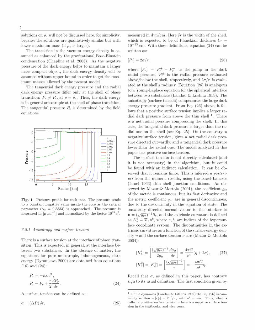
Fig. 1 Pressure profile for each star. The pressure tendsto a constant negative value inside the core as the criticalparameter (αc = 0.5533) is approached. The pressure ismeasured in [g cm−3] and normalized by the factor 1013 c2.

3.2.1 Anisotropy and surface tension

There is a surface tension at the interface of phase tran-

sition. This is expected, in general, at the interface be-tween two substances. In the absence of matter, the

equations for pure anisotropic, inhomogeneous, dark

energy (Dymnikova 2000) are obtained from equations

(16) and (24):

Pr = −ρdec2 ,

Pt = Pr +r

2

dPr

dr. (24)

A surface tension can be defined as:

σ = (∆P ) δr, (25)

measured in dyn/cm. Here δr is the width of the shell,

which is expected to be of Planckian thickness lP ∼10−33 cm. With these definitions, equation (24) can be

written as:

[Pr] = 2σ/r , (26)

where [Pr ] = P+r − P−

r , is the jump in the darkradial pressure, P±

r is the radial pressure evaluated

above/below the shell, respectively, and 2σ/r is evalu-

ated at the shell’s radius r. Equation (26) is analogous

to a Young-Laplace equation for the spherical interface

between two substances (Landau & Lifshitz 1959). Theanisotropy (surface tension) compensates the large dark

energy pressure gradient. From Eq. (26) above, it fol-

lows that a positive surface tension implies a larger ra-

dial dark pressure from above the thin shell 1. Thereis a net radial pressure compressing the shell. In this

case, the tangential dark pressure is larger than the ra-

dial one on the shell (see Eq. 25). On the contrary, a

negative surface tension, gives a net radial dark pres-

sure directed outwardly, and a tangential dark pressurelower than the radial one. The model analyzed in this

paper has positive surface tension.

The surface tension is not directly calculated (and

it is not necessary) in the algorithm, but it couldbe found with an indirect calculation. It can be ob-

served that it remains finite. This is inferred a posteri-

ori from the numeric results, using the Israel-Lanczos

(Israel 1966) thin shell junction conditions. As ob-

served by Mazur & Mottola (2001), the coefficient gttof the metric is continuous, but its first derivative and

the metric coefficient grr are in general discontinuous,

due to the discontinuity in the equation of state. The

outwardly directed normal vector to the interface isn = (

√grr)

−1∂r, and the extrinsic curvature is defined

as Kba = ∇an

b, where a, b, are indices of the hypersur-

face coordinate system. The discontinuities in the ex-

trinsic curvature as a function of the surface energy den-

sity η and the surface tension σ are (Mazur & Mottola2004):

[Ktt ] =

[

(√grr)

−1

2gtt

dgttdr

]

=4πG

c4(η + 2σ) , (27)

[Kθθ ] = [Kφ

φ ] =

[

(√grr)

−1

r

]

= −4πG

c4η.

Recall that σ, as defined in this paper, has contrary

sign to its usual definition. The first condition given by

1In fluid dynamics (Landau & Lifshitz 1959) the Eq. (26) is com-monly written − [Pr] = 2σ′/r , with σ′ = −σ. Thus, what iscalled a positive surface tension σ here is a negative surface ten-sion in the textbooks, and vice versa.

6

Eq. (27) is related to Eq. (26). An assumed jump in

the radial pressure gives a surface tension through Eq.(26), while Eq. (27) gives a jump in the first derivative

of gtt (there is no jump in grr, since it is assumed that

η = 0). Conversely a jump in the first derivative of gttis proportional to a surface tension, and this could becalculated after obtaining the numeric solution (see the

next section). The equation (26) is valid at the shell

even when the isotropic fermion matter is included. In

this case, the stress-energy tensor as a distribution val-

ued tensor is,

Tαβ = Θ(l)T+αβ +Θ(−l)T−

αβ + δ(l)Sαβ , (28)

where the symbols have the usual meaning, and l de-

notes the proper distance along geodesics from the hy-

persurface (see Poisson 2004, for definitions). The sur-face stress-energy tensor is:

Sab = η uaub − σ (hab + uaub) , (29)

in the present case is enough to set η = 0, and to choose

σ to cancel the term −c4 ([Kab]− [K]hab) /8π (the “left

hand side” of Einstein equations). Its components weregiven in Eq. (27). This is the standard procedure for

dealing with thin shells in general relativity Poisson

(2004).

A word of caution is worth mentioning. It is possi-ble to derive an expression, from equations (24) and

(24), for the tangential dark energy pressure at the

shell, analogous to that obtained by Poisson & Israel

(1988):

Pt = −ρde c2 θ(a− r) +

1

2ρde c

2 a δ(r − a) , (30)

where a is the radius of the shell. They pointed outthat this expression becomes singular at the event hori-

zon. In fact, as they showed, a change in variables gives

δ(r − a) = [grr(a)]1/2 δ(s), in terms of the proper dis-

tance s from the shell. So, if r = a is light-like thepressure becomes singular, “even when considered as a

distribution” (Poisson & Israel 1988). This means that

the thin shell of phase transition cannot be located ex-

actly at the event horizon, but can be located elsewhere.

Although this conclusion was originally obtained by aprecursor idea of the dark energy stellar models, it is of

course, applicable to the models studied here.

4 Numeric algorithm

The discontinuity in the dark pressure is managed as

follows: the radial derivative of the total pressure in

0 5 10 15 200

5

10

15

20

25

30

0.55331 0.5533 0.5532 0.552 0.551 0.5 0.4 0.3 0

Den

sity

Radius [km]

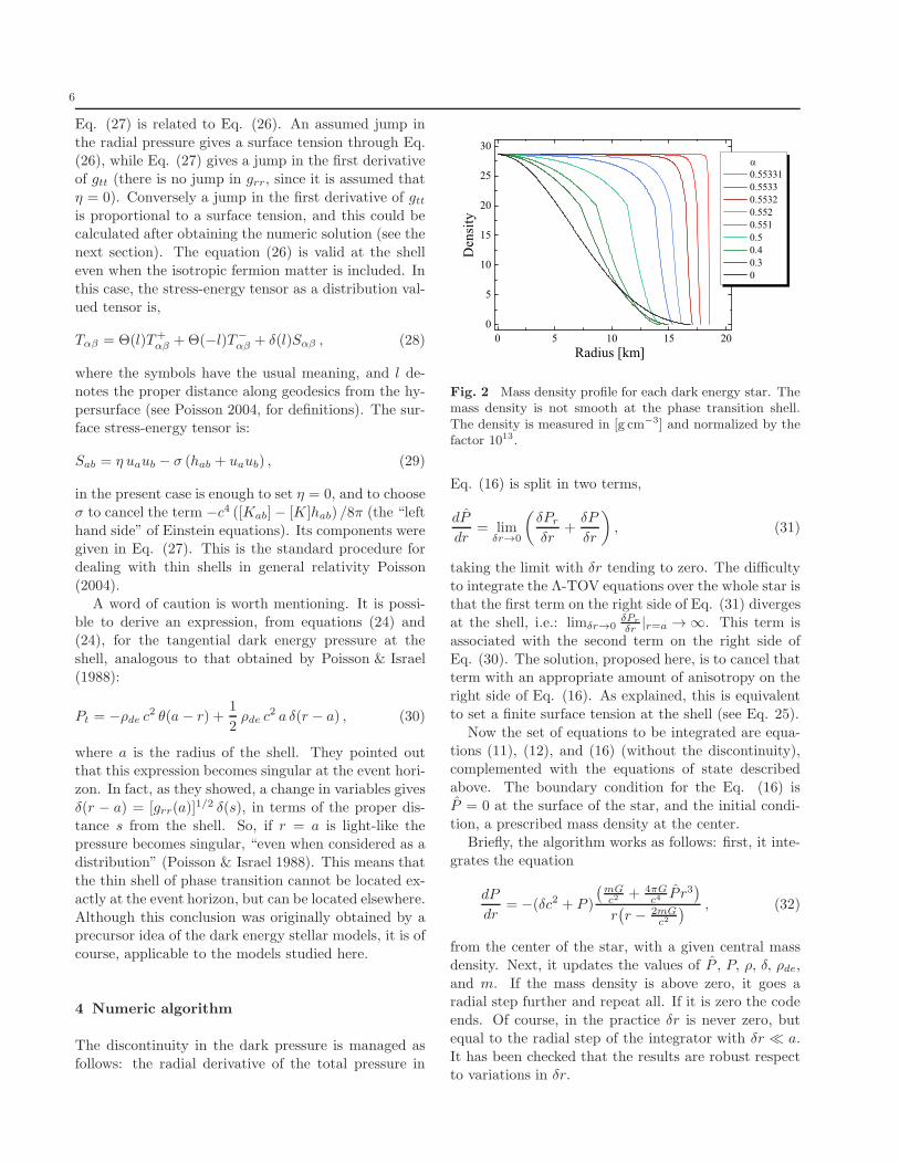
Fig. 2 Mass density profile for each dark energy star. Themass density is not smooth at the phase transition shell.The density is measured in [g cm−3] and normalized by thefactor 1013.

Eq. (16) is split in two terms,

dP

dr= lim

δr→0

(

δPr

δr+

δP

δr

)

, (31)

taking the limit with δr tending to zero. The difficulty

to integrate the Λ-TOV equations over the whole star isthat the first term on the right side of Eq. (31) diverges

at the shell, i.e.: limδr→0δPr

δr |r=a → ∞. This term is

associated with the second term on the right side of

Eq. (30). The solution, proposed here, is to cancel thatterm with an appropriate amount of anisotropy on the

right side of Eq. (16). As explained, this is equivalent

to set a finite surface tension at the shell (see Eq. 25).

Now the set of equations to be integrated are equa-

tions (11), (12), and (16) (without the discontinuity),complemented with the equations of state described

above. The boundary condition for the Eq. (16) is

P = 0 at the surface of the star, and the initial condi-

tion, a prescribed mass density at the center.Briefly, the algorithm works as follows: first, it inte-

grates the equation

dP

dr= −(δc2 + P )

(

mGc2 + 4πG

c4 P r3)

r(

r − 2mGc2

) , (32)

from the center of the star, with a given central mass

density. Next, it updates the values of P , P, ρ, δ, ρde,

and m. If the mass density is above zero, it goes aradial step further and repeat all. If it is zero the code

ends. Of course, in the practice δr is never zero, but

equal to the radial step of the integrator with δr ≪ a.

It has been checked that the results are robust respectto variations in δr.

7

Note that the Eq. (32) is different from the Eq. (16).The term dPr/dr was canceled by a surface tension σ

so that δPr = 2σ/r.

Equations (11), (12), and (16) are integrated with aRunge-Kutta algorithm of the fourth order. The em-

ployed code HE05v2 is an update of the previous code

HE05v1 (see Ghezzi 2005, for more details).

0 5 10 150,0

0,2

0,4

0,6

0,8

1,0

Radius [km]

g rr-1

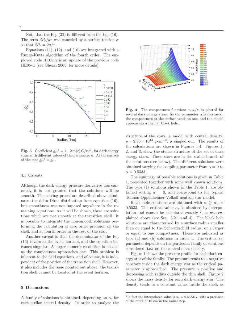
Fig. 3 Coefficient g−1rr = 1−2m(r)G/r c2, for dark energy

stars with different values of the parameter α. At the surfaceof the star g−1

rr = gtt.

4.1 Caveats

Although the dark energy pressure derivative was can-

celed, it is not granted that the solutions will be

smooth. The solving procedure described above elimi-nates the delta Dirac distribution from equation (16),

but smoothness was not imposed anywhere in the re-

maining equations. As it will be shown, there are solu-tions which are not smooth at the transition shell. It

is possible to integrate the non-smooth solutions per-

forming the calculation at zero order precision on theshell, and at fourth order in the rest of the star.

Another caveat is that the denominator of the Eq.

(16) is zero at the event horizon, and the equation be-comes singular. A larger numeric resolution is needed

as the compactness approaches one. This problem is

inherent to the field equations, and of course, it is inde-pendent of the position of the transition shell. However,

it also includes the issue pointed out above: the transi-

tion shell cannot be located at the event horizon.

5 Discussions

A family of solutions is obtained, depending on α, foreach stellar central density. In order to analyze the

04

812

1620 0.0

0.2

0.4

0.6

0.8

1.0

0.1 0.2 0.3 0.4 0.43 0.46 0.48 0.5 0.51 0.52 0.53 0.535 0.54 0.543 0.546 0.55 0.551 0.552 0.553 0.5531 0.5532 0.5533

compa

ctne

ss

radius

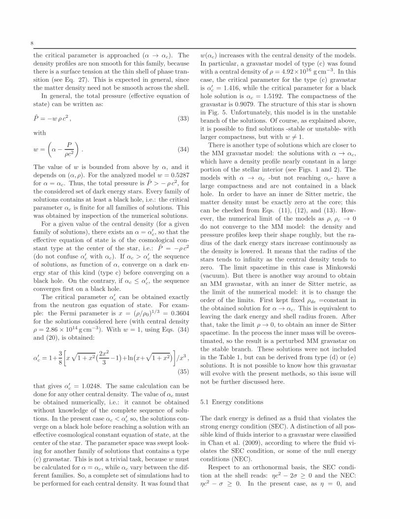
Fig. 4 The compactness function: rsch/r, is plotted forseveral dark energy stars. As the parameter α is increased,the compactness at the surface tends to one, and the modelapproaches a regular black hole.

structure of the stars, a model with central density:

ρ = 2.86× 1014 g cm−3, is singled out. The results of

the calculations are shown in Figures 1-4. Figures 1,

2, and 3, show the stellar structure of the set of darkenergy stars. These stars are in the stable branch of

the solutions (see below). The different solutions were

obtained varying the coupling parameter from α = 0 to

α = 0.5533.The summary of possible solutions is given in Table

1, presented together with some well known solutions.

The type (f) solutions shown in the Table 1, are ob-

tained setting α = 0, and correspond to the typical

Tolman-Oppenheimer-Volkoff neutron star model.Black hole solutions are obtained with α ≥ αc =

0.5533. The critical value αc is obtained by interpo-

lation and cannot be calculated exactly 2, as was ex-

plained above (see Sec. 3.2.1 and 4). The black holesolutions are characterized by a surface radius smaller

than or equal to the Schwarzschild radius, or a larger

or equal to one compactness. These are indicated as

type (a) and (b) solutions in Table 1. The critical αc

parameter depends on the particular family of solutionsconsidered, i.e.: on the central mass density.

Figure 1 shows the pressure profile for each dark en-

ergy star of the family. The pressure tends to a negative

constant inside the dark energy star as the critical pa-rameter is approached. The pressure is positive and

decreasing with radius outside the thin shell. Figure 2

shows the mass density for each dark energy star. The

density tends to a constant value, inside the shell, as

2In fact the interpolated value is αc = 0.553317, with a precisionof the order of 10 cm in the radial step.

8

the critical parameter is approached (α → αc). Thedensity profiles are non smooth for this family, becausethere is a surface tension at the thin shell of phase tran-

sition (see Eq. 27). This is expected in general, sincethe matter density need not be smooth across the shell.

In general, the total pressure (effective equation of

state) can be written as:

P = −w ρ c2 , (33)

with

w =

(

α− P

ρc2

)

. (34)

The value of w is bounded from above by α, and itdepends on (α, ρ). For the analyzed model w = 0.5287for α = αc. Thus, the total pressure is P > − ρ c2, for

the considered set of dark energy stars. Every family ofsolutions contains at least a black hole, i.e.: the criticalparameter αc is finite for all families of solutions. Thiswas obtained by inspection of the numerical solutions.

For a given value of the central density (for a givenfamily of solutions), there exists an α = α′

c, so that theeffective equation of state is of the cosmological con-

stant type at the center of the star, i.e.: P = −ρ c2

(do not confuse α′c with αc). If αc > α′

c the sequenceof solutions, as function of α, converge on a dark en-

ergy star of this kind (type c) before converging on ablack hole. On the contrary, if αc ≤ α′

c, the sequenceconverges first on a black hole.

The critical parameter α′c can be obtained exactly

from the neutron gas equation of state. For exam-ple: the Fermi parameter is x = (ρ/ρ0)

1/3 = 0.3604

for the solutions considered here (with central densityρ = 2.86 × 1014 g cm−3). With w = 1, using Eqs. (34)and (20), is obtained:

α′

c = 1+3

8

[

x√

1 + x2(2x2

3−1

)

+ln(

x+√

1 + x2)

]

/x3 ,

(35)

that gives α′c = 1.0248. The same calculation can be

done for any other central density. The value of αc mustbe obtained numerically, i.e.: it cannot be obtainedwithout knowledge of the complete sequence of solu-

tions. In the present case αc < α′c so, the solutions con-

verge on a black hole before reaching a solution with aneffective cosmological constant equation of state, at the

center of the star. The parameter space was swept look-ing for another family of solutions that contains a type(c) gravastar. This is not a trivial task, because w must

be calculated for α = αc, while αc vary between the dif-ferent families. So, a complete set of simulations had tobe performed for each central density. It was found that

w(αc) increases with the central density of the models.

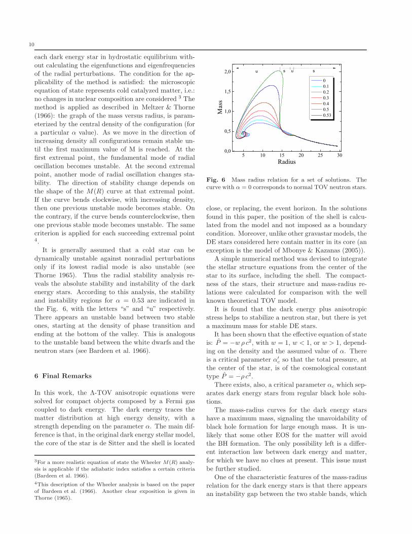
In particular, a gravastar model of type (c) was foundwith a central density of ρ = 4.92×1016 g cm−3. In this

case, the critical parameter for the type (c) gravastar

is α′c = 1.416, while the critical parameter for a black

hole solution is αc = 1.5192. The compactness of thegravastar is 0.9079. The structure of this star is shown

in Fig. 5. Unfortunately, this model is in the unstable

branch of the solutions. Of course, as explained above,

it is possible to find solutions -stable or unstable- withlarger compactness, but with w 6= 1.

There is another type of solutions which are closer to

the MM gravastar model: the solutions with α → αc,

which have a density profile nearly constant in a largeportion of the stellar interior (see Figs. 1 and 2). The

models with α → αc -but not reaching αc- have a

large compactness and are not contained in a black

hole. In order to have an inner de Sitter metric, thematter density must be exactly zero at the core; this

can be checked from Eqs. (11), (12), and (13). How-

ever, the numerical limit of the models as ρ, ρc → 0

do not converge to the MM model: the density andpressure profiles keep their shape roughly, but the ra-

dius of the dark energy stars increase continuously as

the density is lowered. It means that the radius of the

stars tends to infinity as the central density tends tozero. The limit spacetime in this case is Minkowski

(vacuum). But there is another way around to obtain

an MM gravastar, with an inner de Sitter metric, as

the limit of the numerical model: it is to change theorder of the limits. First kept fixed ρde =constant in

the obtained solution for α → αc. This is equivalent to

leaving the dark energy and shell radius frozen. After

that, take the limit ρ → 0, to obtain an inner de Sitterspacetime. In the process the inner mass will be overes-

timated, so the result is a perturbed MM gravastar on

the stable branch. These solutions were not included

in the Table 1, but can be derived from type (d) or (e)solutions. It is not possible to know how this gravastar

will evolve with the present methods, so this issue will

not be further discussed here.

5.1 Energy conditions

The dark energy is defined as a fluid that violates the

strong energy condition (SEC). A distinction of all pos-

sible kind of fluids interior to a gravastar were classified

in Chan et al. (2009), according to where the fluid vi-olates the SEC condition, or some of the null energy

conditions (NEC).

Respect to an orthonormal basis, the SEC condi-

tion at the shell reads: ηc2 − 2σ ≥ 0 and the NEC:ηc2 − σ ≥ 0. In the present case, as η = 0, and

9

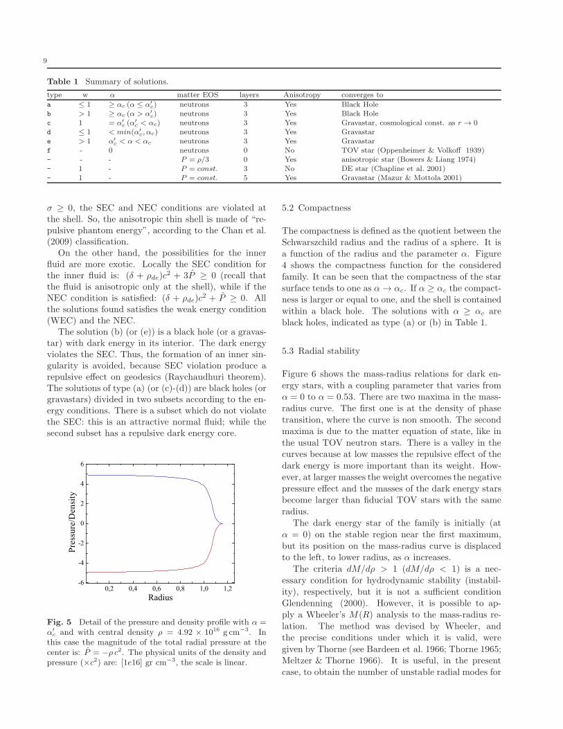
Table 1 Summary of solutions.

type w α matter EOS layers Anisotropy converges to

a ≤ 1 ≥ αc (α ≤ α′

c) neutrons 3 Yes Black Holeb > 1 ≥ αc (α > α′

c) neutrons 3 Yes Black Holec 1 = α′

c (α′

c < αc) neutrons 3 Yes Gravastar, cosmological const. as r → 0d ≤ 1 < min(α′

c, αc) neutrons 3 Yes Gravastare > 1 α′

c < α < αc neutrons 3 Yes Gravastarf - 0 neutrons 0 No TOV star (Oppenheimer & Volkoff 1939)- - - P = ρ/3 0 Yes anisotropic star (Bowers & Liang 1974)- 1 - P = const. 3 No DE star (Chapline et al. 2001)- 1 - P = const. 5 Yes Gravastar (Mazur & Mottola 2001)

σ ≥ 0, the SEC and NEC conditions are violated atthe shell. So, the anisotropic thin shell is made of “re-pulsive phantom energy”, according to the Chan et al.(2009) classification.

On the other hand, the possibilities for the innerfluid are more exotic. Locally the SEC condition forthe inner fluid is: (δ + ρde)c

2 + 3P ≥ 0 (recall thatthe fluid is anisotropic only at the shell), while if theNEC condition is satisfied: (δ + ρde)c

2 + P ≥ 0. Allthe solutions found satisfies the weak energy condition(WEC) and the NEC.

The solution (b) (or (e)) is a black hole (or a gravas-tar) with dark energy in its interior. The dark energyviolates the SEC. Thus, the formation of an inner sin-gularity is avoided, because SEC violation produce arepulsive effect on geodesics (Raychaudhuri theorem).The solutions of type (a) (or (c)-(d)) are black holes (orgravastars) divided in two subsets according to the en-ergy conditions. There is a subset which do not violatethe SEC: this is an attractive normal fluid; while thesecond subset has a repulsive dark energy core.

0,2 0,4 0,6 0,8 1,0 1,2-6

-4

-2

0

2

4

6

Pre

ssur

e/D

ensi

ty

Radius

Fig. 5 Detail of the pressure and density profile with α =α′

c and with central density ρ = 4.92 × 1016 g cm−3. Inthis case the magnitude of the total radial pressure at thecenter is: P = −ρ c2. The physical units of the density andpressure (×c2) are: [1e16] gr cm−3, the scale is linear.

5.2 Compactness

The compactness is defined as the quotient between the

Schwarszchild radius and the radius of a sphere. It isa function of the radius and the parameter α. Figure

4 shows the compactness function for the considered

family. It can be seen that the compactness of the star

surface tends to one as α → αc. If α ≥ αc the compact-ness is larger or equal to one, and the shell is contained

within a black hole. The solutions with α ≥ αc are

black holes, indicated as type (a) or (b) in Table 1.

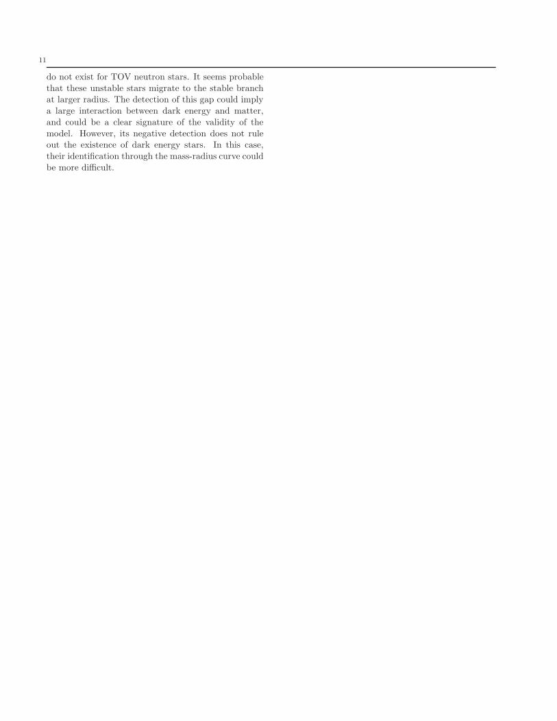
5.3 Radial stability

Figure 6 shows the mass-radius relations for dark en-

ergy stars, with a coupling parameter that varies fromα = 0 to α = 0.53. There are two maxima in the mass-

radius curve. The first one is at the density of phase

transition, where the curve is non smooth. The second

maxima is due to the matter equation of state, like in

the usual TOV neutron stars. There is a valley in thecurves because at low masses the repulsive effect of the

dark energy is more important than its weight. How-

ever, at larger masses the weight overcomes the negative

pressure effect and the masses of the dark energy starsbecome larger than fiducial TOV stars with the same

radius.

The dark energy star of the family is initially (at

α = 0) on the stable region near the first maximum,

but its position on the mass-radius curve is displacedto the left, to lower radius, as α increases.

The criteria dM/dρ > 1 (dM/dρ < 1) is a nec-

essary condition for hydrodynamic stability (instabil-

ity), respectively, but it is not a sufficient conditionGlendenning (2000). However, it is possible to ap-

ply a Wheeler’s M(R) analysis to the mass-radius re-

lation. The method was devised by Wheeler, and

the precise conditions under which it is valid, were

given by Thorne (see Bardeen et al. 1966; Thorne 1965;Meltzer & Thorne 1966). It is useful, in the present

case, to obtain the number of unstable radial modes for

10

each dark energy star in hydrostatic equilibrium with-

out calculating the eigenfunctions and eigenfrequenciesof the radial perturbations. The condition for the ap-

plicability of the method is satisfied: the microscopic

equation of state represents cold catalyzed matter, i.e.:

no changes in nuclear composition are considered 3 Themethod is applied as described in Meltzer & Thorne

(1966): the graph of the mass versus radius, is param-

eterized by the central density of the configuration (for

a particular α value). As we move in the direction ofincreasing density all configurations remain stable un-

til the first maximum value of M is reached. At the

first extremal point, the fundamental mode of radial

oscillation becomes unstable. At the second extremalpoint, another mode of radial oscillation changes sta-

bility. The direction of stability change depends on

the shape of the M(R) curve at that extremal point.

If the curve bends clockwise, with increasing density,then one previous unstable mode becomes stable. On

the contrary, if the curve bends counterclockwise, then

one previous stable mode becomes unstable. The same

criterion is applied for each succeeding extremal point4.

It is generally assumed that a cold star can be

dynamically unstable against nonradial perturbations

only if its lowest radial mode is also unstable (seeThorne 1965). Thus the radial stability analysis re-

veals the absolute stability and instability of the dark

energy stars. According to this analysis, the stability

and instability regions for α = 0.53 are indicated inthe Fig. 6, with the letters “s” and “u” respectively.

There appears an unstable band between two stable

ones, starting at the density of phase transition and

ending at the bottom of the valley. This is analogousto the unstable band between the white dwarfs and the

neutron stars (see Bardeen et al. 1966).

6 Final Remarks

In this work, the Λ-TOV anisotropic equations were

solved for compact objects composed by a Fermi gas

coupled to dark energy. The dark energy traces the

matter distribution at high energy density, with astrength depending on the parameter α. The main dif-

ference is that, in the original dark energy stellar model,

the core of the star is de Sitter and the shell is located

3For a more realistic equation of state the Wheeler M(R) analy-sis is applicable if the adiabatic index satisfies a certain criteria(Bardeen et al. 1966).

4This description of the Wheeler analysis is based on the paperof Bardeen et al. (1966). Another clear exposition is given inThorne (1965).

5 10 15 20 25 300,0

0,5

1,0

1,5

2,0

0 0.1 0.2 0.3 0.4 0.5 0.53

Mas

s

Radius

u

u s u su

Fig. 6 Mass radius relation for a set of solutions. Thecurve with α = 0 corresponds to normal TOV neutron stars.

close, or replacing, the event horizon. In the solutions

found in this paper, the position of the shell is calcu-lated from the model and not imposed as a boundary

condition. Moreover, unlike other gravastar models, the

DE stars considered here contain matter in its core (an

exception is the model of Mbonye & Kazanas (2005)).

A simple numerical method was devised to integratethe stellar structure equations from the center of the

star to its surface, including the shell. The compact-

ness of the stars, their structure and mass-radius re-

lations were calculated for comparison with the wellknown theoretical TOV model.

It is found that the dark energy plus anisotropic

stress helps to stabilize a neutron star, but there is yet

a maximum mass for stable DE stars.

It has been shown that the effective equation of stateis: P = −w ρ c2, with w = 1, w < 1, or w > 1, depend-

ing on the density and the assumed value of α. There

is a critical parameter α′c so that the total pressure, at

the center of the star, is of the cosmological constanttype P = −ρ c2.

There exists, also, a critical parameter αc which sep-

arates dark energy stars from regular black hole solu-

tions.

The mass-radius curves for the dark energy starshave a maximum mass, signaling the unavoidability of

black hole formation for large enough mass. It is un-

likely that some other EOS for the matter will avoid

the BH formation. The only possibility left is a differ-ent interaction law between dark energy and matter,

for which we have no clues at present. This issue must

be further studied.

One of the characteristic features of the mass-radius

relation for the dark energy stars is that there appearsan instability gap between the two stable bands, which

11

do not exist for TOV neutron stars. It seems probable

that these unstable stars migrate to the stable branchat larger radius. The detection of this gap could imply

a large interaction between dark energy and matter,

and could be a clear signature of the validity of the

model. However, its negative detection does not ruleout the existence of dark energy stars. In this case,

their identification through the mass-radius curve could

be more difficult.

12

References

Novikov, I. D., & Frolov, V. P. 1989, Physics of Black Holes,Kluwer Academic Publishers, Dordrecht.

Gliner, E. B. 1966, Sov. Phys. JETP, 22, 378.Gliner, E. B., & Dymnikova, I. G. 1975, Soviet Astronomy

Letters, 1, 93.Poisson, E., & Israel, W. 1988, Class. Quantum Grav., 5,

L201.Chapline, G., Hohlfield, E., Laughlin, R. B., & Santiago, D.

I. 2001, Philos. Mag. B, 81, 235-254.Chapline, G., Hohlfield, E., Laughlin, R. B., & Santiago, D.

I. 2003, “Quantum phase transitions and the breakdownof classical general relativity”, Int. J. Mod Phys. A, 18,3587-3590.

Mazur, P. O., & Mottola, E. 2001, Phys. Rev. D, 64, 104022.Mazur, P. O., & Mottola, E. 2004, Gravitational vacuum

condensate stars, Proc. Nat. Acad. Sci., 101, 9545-9550.Nicolini, P. 2009, “Noncommutative Black Holes, The Final

Appeal To Quantum Gravity: A Review”, Int. J. Mod.Phys. A, 24, 1229; arXiv: 0807.1939 [hep-th].

Nicolini, P., Smailagic, A., & Spallucci, E. 2006, “Noncom-mutative geometry inspired Schwarzschild black hole”,Phys. Lett. B, 632, 547; arXiv: gr-qc/0510112.

Weinberg, S. 1989, Rev. Mod. Phys., 61, 1.Dymnikova, I. G. 2002, “The cosmological term as a source

of mass”, Class. Quantum Grav., 19, 725-739Dymnikova, I. G., “The algebraic structure of a cosmolog-

ical term in spherical symmetric solutions” 2000, Phys.Letters B, 472, 33-38.

Hawking, S. W., & Ellis, G. F. R. 1973, “The Large ScaleStructure of Space-Time”, Cambridge University Press,Cambridge.

Cattoen, C., Faber, T., & Visser, M. 2005, Class. QuantumGravity, 22, 4189-4202.

Mbonye, M. R., & Kazanas. D. 2005, Phys. Rev. D, 72,024016.

Chirenti, C. B. M. H., & Rezzolla, L. 2007, “How to tell agravastar from a black hole”, Class. Quantum Grav.,24,4191-4206.

Chan, V., da Silva, M. F. A., Rocha, P., & Wang, A. 2009,JCAP, 3, 010.

Lobo, F. S. N. 2006, Class. and Quantum Grav., 23, 1525.Broderick, A. E., & Narayan, R. 2007, Class. Quantum

Grav., 24, 659.Barbieri, J., & Chapline, G. 2004, Physics Letters B, 590,

8.Weinberg, S. 1972, “Gravitation and Cosmology: Princi-

ples ans Applications of the General Theory of Relativ-ity”, JohnWiley & Sons, New York; Chichester; Brisbane;Toronto; Singapore.

Poisson, E. A. 2004, “A Relativist’s Toolkit: The Mathe-matics of Black-Hole Mechanics”, Cambridge UniversityPress.

Shapiro, S. L., & Teukolsky, S. A. 1983, “Black holes, whitedwarfs, and neutron stars: The physics of compact ob-jects”, Wiley-Interscience.

Ghezzi, C. R. 2005, Phys. Rev. D, 72, 104017.Bowers, R. L., & Liang, E. P. T. 1974, ApJ, 188, 657.Oppenheimer, J. R., & Volkoff, G. M. 1939, Phys. Rev. D,

55, 374.

Glendenning, N. K. 2000, “Compact Stars”, A&A Library,Springer-Verlag, New York.

Landau, L. D., & Lifshitz, E. 1959, “Fluid mechanics”, Perg-amon Press, Oxford.

Israel, W. 1966, “Singular hypersurfaces and thin shells ingeneral relativity”, Nuovo Cimento, B 44, 1, erratum Is-rael, W. 1967, B 48, 463.

Sagert, I., Fischer, T., Hempel, M., Pagliara, G., Schaffner-Bielich, J., Mezzacappa, A., Thielemann, F. -K., &Liebendorfer, M. 2009, “Strange quark matter in explo-sive astrophysical systems”, Phys. Rev. Lett., 102.

Bardeen, J. M., Thorne, K. S., & Meltzer, D. W. 1966, ApJ,145, 505.

Meltzer, D. W., & Thorne, K. S. 1966, ApJ, 145, 514.Thorne, K. S. 1965, Science, 150, 1671.

This manuscript was prepared with the AAS LATEX macros v5.2.