Computational Statistics & Data Analysis 51 (2007) 6488–6497www.elsevier.com/locate/csda

The Koul–Susarla–Van Ryzin and weighted least squares estimatesfor censored linear regression model: A comparative study

Yanchun Baoa,∗, Shuyuan Heb, Changlin Meic

aSchool of Mathematics, Manchester University, Manchester, M13 9PL, UKbSchool of Mathematical Sciences, Peking University, Beijing, People’s Republic of ChinacSchool of Science, Xi’an Jiaotong University, Xi’an 710049, People’s Republic of China

Received 19 November 2005; received in revised form 25 February 2007; accepted 25 February 2007Available online 5 March 2007

Abstract

The Koul–Susarla–Van Ryzin (KSV) and weighted least squares (WLS) methods are simple to use techniques for handling linearregression models with censored data. They do not require any iterations and standard computer routines can be employed for modelfitting. Emphasis has been given to the consistency and asymptotic normality for both estimators, but the finite sample performanceof the WLS estimator has not been thoroughly investigated. The finite sample performance of these two estimators is comparedusing an extensive simulation study as well as an analysis of the Stanford heart transplant data. The results demonstrate that theWLS approach performs much better than the KSV method and is reliable for use with censored data.© 2007 Elsevier B.V. All rights reserved.

Keywords: Censored data; Linear regression model; Weighted least squares; Stanford heart transplant data

1. Introduction

Let Y be a response variable and Z= (Z1, Z2, . . . , Zr)′ be a random vector of covariates. Assume that Y and Z follow

a linear regression model

Y = b′Z + �, (1)

where b = (b1, b2, . . . , br )′ is the vector of parameters and �, uncorrelated with Z, is the error term with mean zero and

variance �2� . When the response Y is subject to random right censoring, we only observe (Ui, Zi, �i ), i = 1, 2, . . . , n,

which are n replications of (U, Z, �), where U =min(Y, C), �=I [Y �C] and C is the censoring random variable whichis independent of the response Y. Note the censoring works both ways: if � = 0, then the response Y is censored by thecensoring variable C; if � = 1, on the other hand, the censoring variable C is censored by the response Y. The censoredregression problems focus on estimating the parameter vector b and investigating the related statistical properties ofthe estimators based on the observations (Ui, Zi, �i ), i = 1, 2, . . . , n.

Many techniques have been proposed for handling the above regression problems. One methodology in this aspectis based on the synthetic data and uses the ordinary least squares procedure to obtain an estimator of b. It includes

∗ Corresponding author.E-mail addresses: ybao@maths.man.ac.uk (Y. Bao), syhe@maths.pku.edu.cn (S. He), clmei@mail.xjtu.edu.cn (C. Mei).

0167-9473/$ - see front matter © 2007 Elsevier B.V. All rights reserved.doi:10.1016/j.csda.2007.02.025

Y. Bao et al. / Computational Statistics & Data Analysis 51 (2007) 6488–6497 6489

Miller’s estimator (Miller, 1976), Buckley and James’ estimator (Buckley and James, 1979; James and Smith, 1984;Jin et al., 2006), Leurgans’ estimator (Leurgans, 1987; Zhou, 1992a) and in this paper the so-called KSV estimator(Koul et al., 1981; Srinivasan and Zhou, 1994; Fygenson and Zhou, 1992, 1994; Lai et al., 1995). Another estimationmethod is the weighted least squares estimate (abbreviated as WLS in this paper) (Stute, 1993, 1996; He and Wong,2003). In the former methodology, the KSV approach is the easiest to be carried out because no iterations are requiredand standard least squares computer routines can be used once the observations of the response are transformed bythe censoring information. Similar advantages are also achieved by the WLS method. Although much work has beendevoted to the study of the statistical properties such as consistency and asymptotic normality, respectively, for thesetwo methods (see above references), it makes sense to compare their finite sample performance. This paper serves thispurpose by means of an extensive simulation study and an analysis of the Stanford heart transplant data.

The remains of this paper are organized as follows. In Section 2, both the KSV and WLS procedures for linearregression models with censored data are briefly described and some theoretical properties of the estimators such asconsistency and asymptotic normality are also summarized. Extensive simulations are conducted in Section 3 to comparethe finite sample performance of these two estimators under various censoring patterns and underlying distributions ofthe covariates and error term. In Section 4, the famous Stanford heart transplant data are analyzed by these two methodsand the results are compared with those obtained by Miller and Halpern (1982). The paper then concludes with a briefsummary and discussion.

2. The WLS and KSV estimates for censored linear regression models

2.1. Some notations

For any distribution function F(x), let F (x) = 1 − F(x) and (aF , bF ) be the range of F defined by

aF = inf{x : F(x) > 0} and bF = sup{x : F(x) < 1}.Let

F(x) = P(Y �x), G(x) = P(C�x) and H(x, z) = P(Y �x, Z�z) (2)

be the distribution functions of the response Y, censoring variable C and the joint distribution function of Y and thecovariates Z, respectively, where Z = (Z1, Z2, . . . , Zr)

′, z = (z1, z2, . . . , zr )′ and Z�z means that Zi �zi for all

i = 1, 2, . . . , r . Furthermore, we assume throughout the paper that

(i) P (Y �C|Y, Z) = P(Y �C|Y ),

(ii) bF �bG.(3)

As pointed out by Stute (1996), the assumption (i), together with the independence of Y and C, will guarantee that thejoint distribution of (Y, Z) can be theoretically derived from that of (U, Z, �) and consistently estimated from a sample(Ui, Zi , �i ), i = 1, 2, . . . , n. (ii) is a commonly used assumption in the literature of regression with censored data.

2.2. The WLS estimation

The WLS estimator of b and its consistency and asymptotic normality were proposed by Stute (1993, 1996). Fromthe moment estimation viewpoint, He and Wong (2003) obtained the WLS estimator of b as well as the estimator of �2

�and proved the asymptotic normality for both estimators. He and Wong (2003)’s method requires simpler conditionsfor the asymptotic normality of the estimators and provides a more concise form of limit covariance matrix in contrastto that derived by Stute, 1996. Here we briefly describe this method and the related results as follows.

Let

Z0 = Y, Z = (Z1, . . . , Zr)′, � = E(ZZ′) = (�ij )

ri,j=1 and r = (�01, . . . , �0r )

′, (4)

where �ij = E(ZiZj ), 1� i, j �r and �0j = E(YZj ), 1�j �r . Multiplying the two sides of Eq. (1) by Z′ and takingexpectations yields

r = �b. (5)

6490 Y. Bao et al. / Computational Statistics & Data Analysis 51 (2007) 6488–6497

It was derived by He and Wong (2003) that the elements of r and � in (5) can be estimated by

�ij = 1

n

n∑k=1

ZkiZkj�k

1 − Gn(Uk−), 0� i, j �r , (6)

where Zk0 = Uk is the censored observation of Yk , Zk = (Zk1, . . . , Zkr )′ is the observation of the covariate vector Z

corresponding to Yk , Gn(x) is the Kaplan–Meier (KM) estimator for G(x) and Gn(x−) denotes the left continuousversion of Gn(x). Recall that censoring works both ways therefore we can obtain the KM estimator of 1 − G(x) byapplying the KM algorithm to the censored response U, taking 1 − �k instead of �k throughout.

Let � = (�ij )ri,j=1 and r = (�01, . . . , �0r )

′. If we assume that � is invertible, then an estimator of b can be obtainedby

bWLS = �−1

r. (7)

It can easily be checked that the above estimator bWLS is such a vector that minimizes

Q(b) =n∑

k=1

�k

1 − Gn(Uk−)(Uk − b1Zk1 − · · · − brZkr)

2 (8)

and hence is the same WLS estimator as that proposed by Stute (1993). Furthermore, the error variance �2� can be

estimated by

�2� = �00 − b′

WLSr = 1

nQ(bWLS). (9)

We now summarize the strong consistency and asymptotic normality of the estimators bWLS and �2� in the following

two theorems. The first is due to Stute (1993) and the second is due to He and Wong (2003).

Theorem 1. Suppose that � = E(ZZ′) exists and is nonsingular. If Y and C are independent and F and G have nojumps in common, then

limn→∞ bWLS = b a.s.

Theorem 2. Suppose that bothF(x)andG(x)are continuous,� is nonsingular and E[G(Y )]=∫ (1/G(x))F (dx) < ∞.(i) If E[Z2

j �2/G(Y )] < ∞ for all j = 1, 2, . . . , r , then

√n(bWLS − b) converges in distribution as n → ∞ to a

multivariate normal distribution with mean zero and covariance matrix �−1�WLS�−1, where �WLS = (�(w)ij )ri,j=1 and

�(w)ij =

∫gi(y, z)gj (y, z)

G(y)H(dy, dz) −

∫ �i (x)�j (x)

F (x)G2(x)G(dx),

gj (y, z) = zj (y − b′z),

�j (x) =∫

y �x

gj (y, z)H(dy, dz).

(ii) If E[�4/G(Y )] < ∞, then√

n(�2� − �2

� ) converges in distribution as n → ∞ to a normal distribution with meanzero and variance �2

G, where

�2G =

∫h2(y, z)

G(y)H(dy, dz) − �4

� −∫

h2(x)

F (x)G2(x)G(dx),

h(y, z) = (y − b′z)2,

h(x) =∫

y �x

h(y, z)H(dy, dz).

Y. Bao et al. / Computational Statistics & Data Analysis 51 (2007) 6488–6497 6491

2.3. The KSV estimate

Koul et al. (1981) suggested a synthetic data method to handle linear regression models with censored data. Theyconsidered the linear equation

E

[�kUk

1 − G(Uk−)|Zk

]= b′Zk, k = 1, 2, . . . , n (10)

and then substituted G(x) by an estimator G(x), say the KM estimate Gn(x), to obtain the synthetic data

Y ∗k = �kUk

1 − Gn(Uk−), k = 1, 2, . . . , n.

Once Y ∗ are calculated, the standard least squares procedure is used to get the estimator of b as

bKSV =(

n∑k=1

ZkZ′k

)−1 ( n∑k=1

ZkY∗k

), (11)

where Zk = (Zk1, . . . , Zkr )′ is the observation of the covariates corresponding to Yk .

It can be seen that (1/n)∑n

k=1ZkY∗k = (�01, . . . , �0r )

′ = r. Therefore,

bKSV =(

1

n

n∑k=1

ZkZ′k

)−1

r =(

1

n

n∑k=1

ZkZ′k

)−1

�bWLS. (12)

According to the strong law of large numbers and the theorem in Stute (1993, p. 93), if the conditions in Theorem 1hold, then as n → ∞

1

n

n∑k=1

ZkZ′k → � a.s., � → � a.s.

Therefore, the strong consistency of bKSV is obtained.

Theorem 3. Under the assumptions of Theorem 1, we have as n → ∞bKSV → b a.s.

Some work has been devoted to the research of asymptotic normality of the estimator bKSV. Koul et al. (1981)studied the asymptotic normality for bKSV in the case of fixed designs. For random covariates, a similar result hasbeen obtained by Srinivasan and Zhou (1994). It should be noted, however, that these authors only established that√

n(bKSV − bn) has a limiting normal distribution for some bn that converges to b at an unspecific rate. This resultcannot be used, for example, to construct approximate confidence regions for b. Lai et al. (1995) obtained the asymptoticnormality of

√n(bKSV − b) under the more general sense of estimating equations. Nevertheless, their proof requires

some strong assumptions which are not easy to be verified in practice. Furthermore, their covariance matrix of thelimiting distribution is rather complicated.

In light of the relationship between bKSV and bWLS reflected in (12) and along the line of reasoning in He and Wong(2003), Bao (2002) has proved the asymptotic normality for

√n(bKSV − b) under rather simple conditions. This result

is described in the following theorem.

Theorem 4. Suppose that both F(x) and G(x) are continuous, � is nonsingular and E[G(Y )]=∫ (1/G(x))F (dx) < ∞.If for 1�j �r ,

E[Z2j Y

2/G(Y )] < ∞ and E(Z4j ) < ∞,

6492 Y. Bao et al. / Computational Statistics & Data Analysis 51 (2007) 6488–6497

then√

n(bKSV − b) converges in distribution as n → ∞ to a multivariate normal distribution with mean zero andcovariance matrix �−1�KSV�−1, where �KSV = (�(k)

ij )ri,j=1 and

�(k)ij =

∫[Vi(y, z)Vj (y, z)G(y) + fi(z)fj (z)G(y)]H(dy, dz)

−∫

Aj(x)Ai(x) − Aj (x)Ai(x)

F (x)G2(x)G(dx),

Vj (y, z) = gj (y, z)

G(y)+ fj (z),

Aj(x) =∫

y �x

[gj (y, z) + (fj (z) − �j )G(y)]H(dy, dz),

Aj (x) =∫

y �x

(fj (z) − �j )G(y)H(dy, dz),

fj (z) = −zj b′z, gj (y, z) = zj y, �j =∫

fj (z)H(dy, dz).

2.4. Comparison of KSV and WLS

If we let wk = �k/(1 − Gn(Uk−)), we can rewrite the KSV estimator bKSV in (11) and WLS estimator bWLS in (7)as follows:

bKSV =(

n∑k=1

ZkZ′k

)−1 ( n∑k=1

wkZkYk

), bWLS =

(n∑

k=1

wkZkZ′k

)−1 ( n∑k=1

wkZkYk

).

From the above expressions we can clearly see that the KSV estimator is based on the weighted responses whilstthe WLS estimator incorporates both the weighted responses and weighted covariates. Therefore when the censoringmechanism depends on covariates, a false result for the KSV estimator may arise because only the responses areweighted by censoring distribution estimates; the covariates remain unchanged. This situation may be avoided by theuse of the WLS estimator due to both responses and covariates being weighted by the censoring distribution estimates.This is also observed in the simulation study.

3. A simulation study

3.1. Motivation and schemes of simulation study

Although both the WLS and KSV methods provide parameter estimators with good asymptotic properties, an impor-tant aspect to take into consideration is their finite sample performances, which, in practice, may be different betweenthe two. We shall therefore conduct some simulations in this section to compare the finite sample performance of thetwo methods. In general, the estimates may be influenced by several factors, such as, sample size, censoring mecha-nism, distributions of covariates, number of parameters, different models, etc. Our aim is to compare WLS and KSVestimators under various situations by fixing some factors and changing other factors. The following four classes ofsimulations are performed:

(i) For a given model and some specific distributions of the covariates and the error term, the parameters of themodel are estimated by the WLS and KSV methods under various sample sizes and different types of censoringdistributions.

(ii) For a fixed sample size and specific distributions of the censoring variable and error term, the simulations areperformed for different dimensional parameters and different distributions of covariates in the model.

(iii) For a fixed sample size, the simulations are carried out under different censoring distributions and different modelswith the intercept term and/or correlated covariates.

Y. Bao et al. / Computational Statistics & Data Analysis 51 (2007) 6488–6497 6493

(iv) For a fixed sample size and a specific model as well as some specific distributions of the covariates and error term,the simulations are conducted under different censoring percentages, where the censoring variable is dependenton the covariates.

The above four classes cover almost all possible situations we may meet in practice. We also choose the absolutevalues of parameters which are either not too dissimilar such as in classes (i), (ii) and (iv) or extremely different as inclass (iii) (Models (e) and (f)) to check if the values of the parameters may influence the performance of the estimator.

3.2. Simulation results

For the first class of simulations, data were generated from

Model (a) : Y = 0.5Z1 + 2Z2 + �,

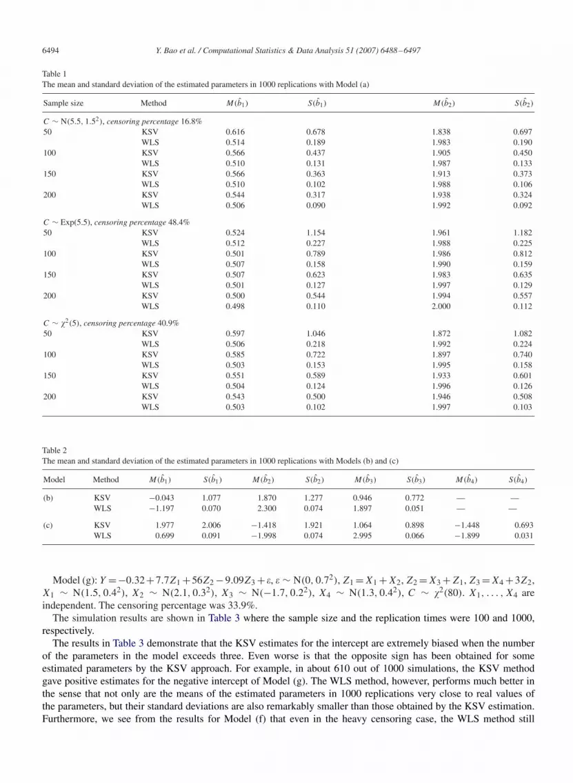
where Z1 ∼ N(1.5, 0.42), Z2 ∼ N(1.5, 0.42), cov(Z1, Z2)=0 and � ∼ N(0, 0.62). The same distribution for covariateswas chosen to check if the parameters can be properly identified. We took the sample size n to be 50, 100, 150 and200, respectively. The censoring distributions are normal N(5.5, 1.52), exponential Exp(5.5) and �2-distribution �2(5),respectively, in which the expectations are similar while the variances are different, yielding different censor percentages.m = 1000 replications were carried out and the mean as well as the standard deviation of the estimated values for eachparameter in the 1000 replications were computed. If we denote by M(bi) and S(bi) the aforementioned two quantities,respectively, then

M(bi) = 1

m

m∑k=1

bik and S(bi) =[

1

m − 1

m∑k=1

(bik − M(bi))2

]1/2

, (13)

which are the estimators of E(bi) and√

Var(bi). These quantities will be used to show how the WLS and KSV estimatorsperform. The results are presented in Table 1.

The results in Table 1 indicate that the WLS method outperforms the KSV method for each sample size and censoringdistribution specified in the simulations. Both the bias and the standard deviation for KSV estimator are generally muchlarger than those obtained by WLS method. And the standard deviations of the KSV estimator are generally five timesas large as those of the WLS estimator.

For the second class of simulations, we fixed the sample size n = 100, with C ∼ Exp(5.5) and � ∼ N(0, 0.52). Datawere generated from

Model (b): Y = −1.2Z1 + 2.3Z2 + 1.9Z3 + �, andModel (c): Y = 0.7Z1 − 2Z2 + 3Z3 − 1.9Z4 + �,where Z1, . . . , Z4 are independent random variables with distributions Z1 ∼ N(1.5, 0.42), Z2 ∼ U(−2, 2), Z3 ∼

Exp(3) and Z4 ∼ �2(3), respectively. The censoring percentages for Models (b) and (c) were 24–56% (on average40.0%) and 28–59% (on average 41.9%), respectively. m = 1000 replications were run and the results are shown inTable 2.

The results given by Table 2 once again show that the WLS estimator performs much better than the KSV estimatorunder the moderate censoring percentages. Compared to the results in Table 1, the KSV estimates are remarkably biasedand the standard deviations become considerably large as the number of the parameters increase. On the contrary, thestandard deviations of the WLS estimator seem very stable and much smaller than those of the KSV estimator.

The four models with related issues for the third class of simulations are listed as follows:Model (d): Y = −2 + 0.6Z1 + �, � ∼ N(0, 1.52), Z1 ∼ U(2.5, 7), C ∼ Exp(3.3). The censoring percentage

was 25.6%.Model (e): Y =72−1.21Z1−55Z2+0.11Z3+�, � ∼ N(0, 1.52), Z1 ∼ N(3.5, 0.32), Z2 ∼ Exp(1.1), Z3 ∼ U(8, 16),

C ∼ N(9, 0.62). Z1, Z2, Z3 are independent. The censoring percentage was 63.0%.Model (f): Y = 0.55 − 6.82Z1 + 13Z2 − 0.09Z3 + �, � ∼ N(0, 0.82), Z1 = X1, Z2 = 2X1 + X2, Z3 = X3,

X1 ∼ U(2.5, 7), X2 ∼ Exp(1.2), X3 ∼ U(−13, 5), C ∼ N(86, 1.52). X1, X2, X3 are independent. The censoringpercentage was 73.3%.

6494 Y. Bao et al. / Computational Statistics & Data Analysis 51 (2007) 6488–6497

Table 1The mean and standard deviation of the estimated parameters in 1000 replications with Model (a)

Sample size Method M(b1) S(b1) M(b2) S(b2)

C ∼ N(5.5, 1.52), censoring percentage 16.8%50 KSV 0.616 0.678 1.838 0.697

WLS 0.514 0.189 1.983 0.190100 KSV 0.566 0.437 1.905 0.450

WLS 0.510 0.131 1.987 0.133150 KSV 0.566 0.363 1.913 0.373

WLS 0.510 0.102 1.988 0.106200 KSV 0.544 0.317 1.938 0.324

WLS 0.506 0.090 1.992 0.092

C ∼ Exp(5.5), censoring percentage 48.4%50 KSV 0.524 1.154 1.961 1.182

WLS 0.512 0.227 1.988 0.225100 KSV 0.501 0.789 1.986 0.812

WLS 0.507 0.158 1.990 0.159150 KSV 0.507 0.623 1.983 0.635

WLS 0.501 0.127 1.997 0.129200 KSV 0.500 0.544 1.994 0.557

WLS 0.498 0.110 2.000 0.112

C ∼ �2(5), censoring percentage 40.9%50 KSV 0.597 1.046 1.872 1.082

WLS 0.506 0.218 1.992 0.224100 KSV 0.585 0.722 1.897 0.740

WLS 0.503 0.153 1.995 0.158150 KSV 0.551 0.589 1.933 0.601

WLS 0.504 0.124 1.996 0.126200 KSV 0.543 0.500 1.946 0.508

WLS 0.503 0.102 1.997 0.103

Table 2The mean and standard deviation of the estimated parameters in 1000 replications with Models (b) and (c)

Model Method M(b1) S(b1) M(b2) S(b2) M(b3) S(b3) M(b4) S(b4)

(b) KSV −0.043 1.077 1.870 1.277 0.946 0.772 — —WLS −1.197 0.070 2.300 0.074 1.897 0.051 — —

(c) KSV 1.977 2.006 −1.418 1.921 1.064 0.898 −1.448 0.693WLS 0.699 0.091 −1.998 0.074 2.995 0.066 −1.899 0.031

Model (g): Y =−0.32+7.7Z1 +56Z2 −9.09Z3 + �, � ∼ N(0, 0.72), Z1 =X1 +X2, Z2 =X3 +Z1, Z3 =X4 +3Z2,X1 ∼ N(1.5, 0.42), X2 ∼ N(2.1, 0.32), X3 ∼ N(−1.7, 0.22), X4 ∼ N(1.3, 0.42), C ∼ �2(80). X1, . . . , X4 areindependent. The censoring percentage was 33.9%.

The simulation results are shown in Table 3 where the sample size and the replication times were 100 and 1000,respectively.

The results in Table 3 demonstrate that the KSV estimates for the intercept are extremely biased when the numberof the parameters in the model exceeds three. Even worse is that the opposite sign has been obtained for someestimated parameters by the KSV approach. For example, in about 610 out of 1000 simulations, the KSV methodgave positive estimates for the negative intercept of Model (g). The WLS method, however, performs much better inthe sense that not only are the means of the estimated parameters in 1000 replications very close to real values ofthe parameters, but their standard deviations are also remarkably smaller than those obtained by the KSV estimation.Furthermore, we see from the results for Model (f) that even in the heavy censoring case, the WLS method still

Y. Bao et al. / Computational Statistics & Data Analysis 51 (2007) 6488–6497 6495

Table 3The mean and standard deviation of the estimated parameters in 1000 replications for Models (d), (e), (f) and (g) (b0 stands for the intercept)

Model Method M(b0) S(b0) M(b1) S(b1) M(b2) S(b2) M(b3) S(b3)

(d) KSV −1.891 0.867 0.571 0.186 — — — —WLS −1.927 0.726 0.579 0.150 — — — —

(e) KSV 21.138 21.650 −0.028 5.688 −36.698 3.501 0.047 0.753WLS 71.842 3.503 −1.203 0.909 −54.961 0.268 0.112 0.116

(f) KSV 118.817 31.308 −2.235 13.144 −8.027 5.951 −0.002 1.642WLS 0.829 1.442 −6.799 0.691 12.949 0.365 −0.091 0.034

(g) KSV 34.723 123.655 3.724 58.853 21.369 102.803 −3.519 29.047WLS −0.283 1.182 7.695 0.539 55.965 0.961 −9.085 0.261

yields very satisfactory estimates for each of the four parameters except for the estimated intercept which is a littlebit biased.

It has been found that the KSV method provides unreasonable estimates in the case where the censoring variable isdependent on the covariates (see, for example, Miller and Halpern, 1982; Leurgans, 1987; Fygenson and Zhou, 1994). Inorder to examine the performance of the WLS estimator in this case, we carried out some simulations especially designedto access the influence of dependency between the censoring mechanism and the covariates. Data were generated fromModel (a) and the distribution of the error term � is N(0,0.62). We assume Z1 ∼ Exp(5.5), Z2 ∼ N(1.5, 0.42) andthe censoring variable C = Z1 + Z2 + r , where r is a constant. We adjusted r to give different censoring percentages.The sample size was 100 and 1000 replications were run to compute M(bi) and S(bi). The KSV estimates were alsocalculated for comparison. The results are shown in Table 4.

The results in Table 4 confirm that the KSV method yields extremely unreasonable estimates when the censoringvariable is dependent on the covariates. Even in the light censoring cases, there is considerable bias in the estimatedparameters. When the censoring percentage becomes large, the biases and standard deviations of the estimated param-eters increase dramatically and totally misleading results are produced in the heavy censoring cases. The WLS method,however, performs much better than the KSV method. The biases and standard deviations of the WLS estimator areapparently much smaller than those of the KSV estimator. In addition, WLS method provides remarkably more stableestimates as the censoring percentage increases. Even in the heavy censoring cases, the satisfactory estimates are stillgiven by the WLS method.

In conclusion, our simulations indicate that the KSV method may be extremely biased when the censoring variableis dependent on the covariates as well as when the censoring times are i.i.d. and do not vary with the covariates. Thesame findings have also been reported by Fygenson and Zhou (1994). The WLS method, however, yields satisfactoryestimates under various situations although virtually the same weights as those in the KSV method are used. Thedifference between these two methods, as shown in Section 2.4, is that in the KSV method, the weights are only usedto obtain the synthetic data for the response with the corresponding observations of the covariates left unchanged.In the WLS method, however, the weights exert their influence on the observations of the response as well as on thecorresponding observations of the covariates simultaneously.

4. An example

The practical data from the Stanford heart transplant program will be analyzed in this section to further examinethe performance of the KSV and WLS methods. This data set has been used to illustrate many regression tech-niques for censored data, see for example, Miller and Halpern (1982), Hoover and Guess (1990), Zhou (1992b),Currie (1996), Jin et al. (2006). Among others, Miller and Halpern (1982) analyzed this data set using both thelinear regression method and Cox’s proportional hazards model and provided an extensive discussion of the fourregression techniques with censored data, which are due to Cox (1972), Miller (1976), Buckley and James (1979)and Koul et al. (1981).

The Stanford heart transplant program and the resulting data have been fully described in Miller and Halpern (1982). Inorder to compare theWLS technique with other methods, we follow Miller and Halpern (1982) to analyze the dependence

6496 Y. Bao et al. / Computational Statistics & Data Analysis 51 (2007) 6488–6497

Table 4The mean and standard deviation of the estimated parameters in 1000 replications with Model (a) and the censoring variable C = Z1 + Z2 + r

r Censoring percentage Method M(b1) S(b1) M(b2) S(b2)

10.00 0.0 KSV 0.500 0.011 2.001 0.052WLS 0.500 0.011 2.001 0.052

1.80 5.2 KSV 0.605 0.049 1.709 0.130WLS 0.507 0.011 1.951 0.053

1.40 10.5 KSV 0.698 0.065 1.476 0.157WLS 0.511 0.012 1.920 0.057

0.90 20.2 KSV 0.872 0.095 1.068 0.209WLS 0.515 0.013 1.882 0.066

0.45 30.3 KSV 1.073 0.127 0.606 0.261WLS 0.517 0.014 1.858 0.075

0.00 40.2 KSV 1.313 0.171 0.057 0.335WLS 0.518 0.015 1.842 0.088

−0.50 50.0 KSV 1.611 0.222 −0.650 0.425WLS 0.518 0.016 1.833 0.107

−1.15 60.5 KSV 2.066 0.315 −1.787 0.621WLS 0.517 0.019 1.820 0.138

−1.95 70.5 KSV 2.694 0.453 −3.415 0.922WLS 0.516 0.022 1.812 0.180

−3.05 80.2 KSV 3.690 0.734 −6.098 1.655WLS 0.515 0.026 1.802 0.249

−5.00 90.3 KSV 5.841 1.506 −12.165 3.689WLS 0.514 0.046 1.774 0.532

Table 5The estimated coefficients of Models (h) and (i) by the Buckley and James, the Miller, the KSV and the WLS methods

Method Intercept a0 Age a1 Mismatch score a2 Intercept b0 Age b1 Age2 b2

Buckley & James 3.23 −0.015 −0.003 1.35 0.107 −0.0017Millera 2.57 −0.001 0.072

2.54 0.000 0.040KSV 0.72 0.024 0.251 0.798 0.039 −0.0002WLS 2.36 −0.0014 0.091 0.904 0.098 −0.0013

aThe iterative sequences of the estimators trap in a loop with the two sets of values.

of the base 10 logarithm of the survival time T on age at transplant Z1 and on a mismatch score Z2. That is, we considerthe following two models:

Model (h): Y = a0 + a1Z1 + a2Z2 + �, andModel (i): Y = b0 + b1Z1 + b2Z

21 + �,

where Y = log10 T . Like the analysis in Miller and Halpern (1982), the first model was fitted with 157 cases and thesecond model was fitted with 152 cases where the five patients with survival time less than 10 days were omitted.Table 5 presents the estimated coefficients by the WLS and KSV methods together with other results obtained by Millerand Halpern (1982).

It has been pointed out by Miller and Halpern (1982) that the Buckley and James estimator for the heart transplantdata is more reliable than both the Miller and the KSV estimators in the sense that the Buckley and James methodyields a negative slope for the age which has been thought to be reasonable. Miller’s procedure does not converge

Y. Bao et al. / Computational Statistics & Data Analysis 51 (2007) 6488–6497 6497

and falls in a loop with two sets of values whilst the KSV method yields a positive slope for the age. The estimatedcoefficients obtained by the KSV method are also considerably different from those obtained by the other methods.The WLS method, however, yields similar estimates of the coefficients to those by the Buckley and James method, notonly in the signs of the estimated coefficients, but also in their absolute values.

For the quadratic age model, although the same sign for the estimated coefficients has been obtained by all of themethods except for the Miller’s approach, WLS estimates are much closer to Buckley and James estimates than theKSV estimates. The analysis of this empirical example also indicates that the WLS method is superior to the KSVmethod and is comparable to the Buckley and James method.

5. Summary and discussion

After briefly describing the procedures and some theoretical results for the KSV and WLS estimates for the linearregression model with censored data, an extensive simulation study together with an analysis of the Stanford hearttransplant data have been carried out in this paper to examine the finite sample performance of these two methods.Although the algorithm of the WLS estimate is almost as simple as that of the KSV estimate where standard least squarescomputer routines can be used, the above simulation study and the analysis of an empirical data set have indicated thatthe WLS method performs much better than the KSV method, especially when the number of parameters in the modelis large or the censoring is heavy. The empirical example has shown that the WLS method yields estimates as good asthat by the Buckley and James method, as well as being easier to compute compared to the Buckley and James methodbecause no iterations are required. Although the KSV and WLS estimators are all asymptotically normal when thesample size goes to infinity, they indicate very different performances in the case of finite sample size. Nevertheless,the theoretical comparison of these two methods is interesting.

Acknowledgements

The authors thank two anonymous referees as well as the Co-Editor and Associate Editor for their comments andsuggestions. This research was supported by NSFC 10231030 and RFDP.

References

Bao, Y., 2002. The KSV estimate for right censored linear regression. Master Degree Thesis (in Chinese), Peking University.Buckley, J., James, I., 1979. Linear regression with censored data. Biometrika 66, 429–436.Cox, D.R., 1972. Regression models and life-tables (with discussion). J. Roy. Statist. Soc. Ser. B 34, 187–202.Currie, I.D., 1996. A note on Buckley–James estimators for censored data. Biometrika 83, 912–915.Fygenson, M., Zhou, M., 1992. Modification of the Koul–Susarla–Van Ryzin estimator for linear regression models with right censoring. Statist.

Probab. Lett. 13, 295–299.Fygenson, M., Zhou, M., 1994. On using stratification in the analysis of linear regression models with right censoring. Ann. Statist. 22, 747–762.He, S., Wong, X., 2003. The central limit theorem under censoring when covariables are present. Sci. China Ser. A 46, 600–610.Hoover, D.R., Guess, F.M., 1990. Miscellanea response linked censoring: modelling and estimation. Biometrika 77, 893–896.James, I., Smith, P.J., 1984. Consistency results for linear regression with censored data. Ann. Statist. 12, 590–600.Jin, Z., Lin, D.Y., Wei, L.J., Ying, Z., 2006. On least-squares regression with censored data. Biometrika 93, 147–161.Koul, H., Susarla, V., Van Ryzin, J., 1981. Regression analysis with randomly right censored data. Ann. Statist. 9, 1276–1288.Lai, T.L., Ying, Z., Zheng, Z., 1995. Asymptotic normality of a class of adaptive statistics with applications to synthetic data methods for censored

regression. J. Multivariate Anal. 52, 259–279.Leurgans, S., 1987. Linear models, random censoring and synthetic data. Biometrika 74, 301–309.Miller, R., 1976. Least square regression with censored data. Biometrika 63, 449–464.Miller, R., Halpern, J., 1982. Regression with censored data. Biometrika 69, 521–531.Srinivasan, C., Zhou, M., 1994. Linear regression with censoring. J. Multivariate Anal. 49, 179–201.Stute, W., 1993. Consistent estimation under random censorship when covariables are present. J. Multivariate Anal. 45, 89–103.Stute, W., 1996. Distributional convergence under random censorship when covariables are present. Scand. J. Statist. 23, 461–471.Zhou, M., 1992a. Asymptotic normality of the ‘synthetic data’ regression estimator for censored survival data. Ann. Statist. 20, 1002–1021.Zhou, M., 1992b. M-estimation in censored linear models. Biometrika 79, 837–841.