Embed Size (px)
Citation preview
SIAM J. MATRIX ANAL. APPL. c© 2006 Society for Industrial and Applied MathematicsVol. 28, No. 2, pp. 477–502
FAST METHODS FOR ESTIMATING THE DISTANCE TOUNCONTROLLABILITY∗
M. GU† , E. MENGI‡ , M. L. OVERTON‡ , J. XIA† , AND J. ZHU†
Abstract. The distance to uncontrollability for a linear control system is the distance (in the2-norm) to the nearest uncontrollable system. We present an algorithm based on methods of Gu andBurke–Lewis–Overton that estimates the distance to uncontrollability to any prescribed accuracy.The new method requires O(n4) operations on average, which is an improvement over previousmethods which have complexity O(n6), where n is the order of the system. Numerical experimentsindicate that the new method is reliable in practice.
Key words. distance to uncontrollability, complex controllability radius, trisection, real eigen-value extraction, shifted inverse iteration, shift-and-invert Arnoldi, Sylvester equation, Kroneckerproduct
AMS subject classifications. 65F15, 93B05, 65K10
DOI. 10.1137/05063060X
1. Introduction. Given A ∈ Cn×n, B ∈ C
n×m, the linear control system
x = Ax + Bu(1.1)
is controllable if for every pair of states x0, xf ∈ Cn there exists a continuous control
function u(t) to steer the initial state x0 to the final state xf within finite time.Equivalently, according to a well-known result by Kalman [8], the system (1.1) iscontrollable if the matrix [A− λI B] has full row rank for all λ ∈ C.
To measure the conditioning of (1.1), the distance to uncontrollability was intro-duced in [12] as
τ(A,B) = min{‖ΔA ΔB‖ : (A + ΔA,B + ΔB) is uncontrollable},(1.2)
which was later shown to be equivalent to [4, 5]
τ(A,B) = minλ∈C
σn([A− λI B]),(1.3)
where ‖ · ‖ denotes the 2-norm or Frobenius norm1 and σn([A− λI B]) denotes thenth largest singular value of the n × (n + m) matrix [A − λI B]. This is a globalnonsmooth optimization problem in two real variables α and β, the real and imaginaryparts of λ. But note that σn([A − λI B]) is not convex and may have many localminima, so standard optimization methods, which are guaranteed only to converge toa local minimum, will not yield reliable results in general.
∗Received by the editors May 3, 2005; accepted for publication (in revised form) by N. MastronardiDecember 21, 2005; published electronically June 21, 2006.
http://www.siam.org/journals/simax/28-2/63060.html†Department of Mathematics, University of California at Berkeley, Berkeley, CA 94720
([email protected], [email protected], [email protected]). The research oftheseauthors was supported in part by the National Science Foundation grant DMS-0412049.
‡Courant Institute of Mathematical Sciences, New York University, New York, NY 10012 ([email protected], [email protected]). The research of these authors was supported in part by the Na-tional Science Foundation grant CCR-0204388.
1The definitions of τ(A,B) in terms of the Frobenius norm and the 2-norm are equivalent.
477
478 M. GU, E. MENGI, M. L. OVERTON, J. XIA, AND J. ZHU
Gu [6] proposed a bisection method which can correctly estimate τ(A,B) within afactor of 2 in time polynomial in n. Throughout the paper, when we refer to operationcounts we assume that the computation of the eigenvalues of a matrix or pencil is anatomic operation whose cost is cubic in the dimension. Burke, Lewis, and Overton[3] suggested a trisection variant to retrieve the distance to uncontrollability to anydesired accuracy. The methods in these two papers are based on a simultaneouscomparison of two estimates δ1 > δ2 with τ(A,B). More precisely, Gu derived ascheme that returns one of the inequalities
τ(A,B) ≤ δ1(1.4)
and
τ(A,B) > δ2.(1.5)
Even if both of the inequalities are satisfied, Gu’s scheme returns information aboutonly one of the inequalities. Gu’s method depends on the extraction of the realeigenvalues of a pencil of size 2n2 × 2n2 and the imaginary eigenvalues of matrices ofsize 2n×2n. Computationally the verification scheme is dominated by the extractionof the real eigenvalues of the generalized problem of size 2n2 × 2n2, which requiresO(n6) operations if the standard QZ algorithm is used.
In this paper we present an alternative verification scheme for comparisons (1.4)and (1.5). In the new verification scheme we still need to find real eigenvalues of2n2×2n2 matrices, so there is no asymptotic gain over Gu’s verification scheme whenwe use the QR algorithm. Nevertheless, we show that the inverse of these 2n2 × 2n2
matrices shifted by a real number times the identity can be multiplied onto a vectorefficiently by solving a Sylvester equation of size 2n with a cost of O(n3). Therefore,given a real number as the shift, by applying shifted inverse iteration or a shift-and-invert preconditioned Arnoldi method, the closest eigenvalue to the real number canbe obtained by performing O(n3) operations. Motivated by the fact that we needonly real eigenvalues, we provide two alternative ways to scan the real axis to findthe desired eigenvalues. Both of the approaches require an upper bound on the normof the input matrix (of size 2n2 × 2n2) as a parameter. For one of the approaches,which is based on a “divide and conquer” idea, choosing this parameter arbitrarilylarge does not affect the efficiency of the algorithm much. The efficiency of the otherapproach, which we name “adaptive progress,” depends not only on this parametersignificantly but also on another parameter that bounds the distance between theclosest pair of eigenvalues from below. For the divide and conquer approach, weprove that extracting all of the real eigenvalues requires O(n4) operations on averageand O(n5) operations in the worst case. For the adaptive progress approach suchneat results are not immediate because of the dependence of the performance of thealgorithm on the parameters. In practice we observe that the divide and conquerapproach is the more efficient and more reliable method.
In section 2 we will review the trisection method for estimating τ(A,B) and Gu’sscheme for verifying which one of (1.4) and (1.5) holds. In section 3 we presentour modified eigenvalue problem for the same purpose and fast methods based onthe shifted inverse iteration or shift-and-invert Arnoldi for solving it. Specifically,to extract all of the real eigenvalues, we discuss two search strategies: an adaptiveprogress approach and a divide and conquer approach. The effectiveness and reliabilityof the methods are demonstrated by the numerical examples in section 4.
FAST METHODS FOR DISTANCE TO UNCONTROLLABILITY 479
2. Trisection and Gu’s verification scheme.
2.1. Bisection and trisection. The problem of computing the distance to un-controllability is equivalent to the minimization of σn([A − λI B]) over the entirecomplex plane. Gu [6] proposed the first polynomial-time estimation scheme. Burke,Lewis, and Overton [3] later suggested a trisection version to retrieve the distance touncontrollability to an arbitrary accuracy. Given two real numbers δ1 > δ2, at eachiteration both of the algorithms alter an upper bound or a lower bound depending onwhich of the inequalities (1.4) and (1.5) holds. This test is based on the following the-orem [6], which is a consequence of the fact that singular values are well-conditioned(in the absolute sense).
Theorem 2.1 (see Gu [6]). Assume that δ > τ(A,B). Given an η ∈ [0, 2(δ −τ(A,B))], there exist at least two pairs of real numbers α and β such that
δ ∈ σ ([A− (α + βi)I,B]) and δ ∈ σ ([A− (α + η + βi)I,B]) ,(2.1)
where σ(·) denotes the set of singular values of its argument.We shall describe two alternative ways of verifying the existence of a pair α and β
satisfying (2.1) for a given δ and η in subsections 2.2 and 3.1. Suppose we set δ1 = δand δ2 = δ−η/2. The theorem above implies that when no pair satisfying (2.1) existsthe inequality η > 2(δ − τ(A,B)) is satisfied, so condition (1.5) holds. On the otherhand, when a pair exists, then by definition (1.3) we can conclude (1.4).
Gu’s bisection algorithm (Algorithm 1) keeps only an upper bound on the distanceto uncontrollability. It refines the upper bound until condition (1.5) is satisfied. Noticethat in Algorithm 1, δ = η = δ1. At termination the distance to uncontrollability lieswithin factor of 2 of δ1, with δ1/2 < τ(A,B) ≤ 2δ1.
Algorithm 1 Gu’s bisection estimation algorithm
Call: δ1 ← Bisection(A,B).Input: A ∈ C
n×n and B ∈ Cn×m with m ≤ n.
Output: A scalar δ1 satisfying δ1/2 < τ(A,B) ≤ 2δ1.
1. Initialize the estimate as δ1 ← σn([A B])/2.repeatδ2 ← δ1
2 .Apply Gu’s test.if (1.4) is verified thenδ1 ← δ2.done ← FALSE.
else% Otherwise (1.5) is verified.done ← TRUE.
end ifuntil done = TRUE
2. Return δ1.
To obtain the distance to uncontrollability with better accuracy, Burke, Lewis,and Overton [3] proposed a trisection variant. The trisection algorithm (Algorithm 2)bounds τ(A,B) by an interval [l, u] and reduces the length of this interval by a factorof 2
3 at each iteration. Thus it can compute τ(A,B) to any desired accuracy in O(n6)operations which is the cost of Gu’s test, as described next.
480 M. GU, E. MENGI, M. L. OVERTON, J. XIA, AND J. ZHU
Algorithm 2 Trisection variant of Algorithm 1
Call: [l, u] ← Trisection(A,B,ε).Input: A ∈ C
n×n, B ∈ Cn×m with m ≤ n, and a tolerance ε > 0.
Output: Scalars l and u satisfying l < τ(A,B) ≤ u and u− l < ε.
1. Initialize the lower bound as l ← 0 and the upper bound as u ← σn([A B]).repeatδ1 ← l + 2
3 (u− l)
δ2 ← l + 13 (u− l)
Apply Gu’s test.if (1.4) is verified thenu ← δ1.
else% Otherwise (1.5) is verified.l ← δ2.
end ifuntil u− l < ε
2. Return l and u.
2.2. Gu’s verification scheme. By means of Gu’s test we can numericallyverify whether a real pair of solutions to (2.1) exists. Equation (2.1) in Theorem 2.1implies that there exist nonzero vectors
(xy
), z,
(xy
), and z such that
(A− (α + βi)I B )
(xy
)= δz,
(A∗ − (α− βi)I
B∗
)z = δ
(xy
),(2.2a)
(A− (α + η + βi)I B )
(xy
)= δz,
(A∗ − (α + η − βi)I
B∗
)z = δ
(xy
).(2.2b)
These equations can be rewritten as⎛⎝ −δI A− αI B
A∗ − αI −δI 0B∗ 0 −δI
⎞⎠
⎛⎝ z
xy
⎞⎠ = βi
⎛⎝ 0 I 0
−I 0 00 0 0
⎞⎠
⎛⎝ z
xy
⎞⎠(2.3a)
and
⎛⎝ −δI A− (α + η)I B
A∗ − (α + η)I −δI 0B∗ 0 −δI
⎞⎠
⎛⎝ z
xy
⎞⎠ = βi
⎛⎝ 0 I 0
−I 0 00 0 0
⎞⎠
⎛⎝ z
xy
⎞⎠.
(2.3b)
Furthermore using the QR factorization(B−δI
)=
(Q11 Q12
Q21 Q22
)(R0
)(2.4)
these problems can be reduced to standard eigenvalue problems of size 2n× 2n, i.e.,the eigenvalues of the pencils in (2.3a) and in (2.3b) are the same as the eigenvaluesof the matrices (
A− αI BQ22 − δQ12
δQ−112 −Q−1
12 (A∗ − αI)Q12
)(2.5a)
FAST METHODS FOR DISTANCE TO UNCONTROLLABILITY 481
and (A− (α + η)I BQ22 − δQ12
δQ−112 −Q−1
12 (A∗ − (α + η)I)Q12
),(2.5b)
respectively. In order for (2.1) to have at least one real solution (α, β), these twomatrices must share a common pure imaginary eigenvalue βi. This requires a 2n2×2n2
generalized eigenvalue problem to have a real eigenvalue α (see [6]). For a given δ andη, we check whether the latter generalized eigenvalue problem has any real eigenvalueα. If it does, then we check the existence of a real eigenvalue α for which the matrices(2.5a) and (2.5b) share a common pure imaginary eigenvalue βi. There exists a pairof α and β satisfying (2.1) if and only if this process succeeds.
3. Modified fast verification scheme. It turns out that Gu’s verificationscheme can be simplified. In this modified scheme the 2n2 × 2n2 generalized eigen-value problems whose real eigenvalues are sought in Gu’s scheme are replaced by2n2 × 2n2 standard eigenvalue problems, and the 2n× 2n standard eigenvalue prob-lems (2.5a) and (2.5b) whose imaginary eigenvalues are sought are replaced by new2n × 2n standard eigenvalue problems that do not require the computation of QRfactorizations.
The simplification of the problem of size 2n2 × 2n2 is significant, as the inverse ofthe new matrix of size 2n2×2n2 (whose real eigenvalues are sought) times a vector canbe computed in a cheap manner by solving a Sylvester equation of size 2n×2n with acost of O(n3). As a consequence the closest eigenvalue to a given complex point can becomputed efficiently by applying shifted inverse iteration or shift-and-invert Arnoldi.We discuss how this idea can be extended to extract all of the real eigenvalues withan average cost of O(n4) and a worst case cost of O(n5), reducing the running timeof each iteration of the bisection or the trisection algorithm asymptotically.
3.1. New generalized eigenvalue problem. According to (2.2a)
y =1
δB∗z
and the two equations in (2.2a) can be rewritten as(B A− αI
A∗ − αI −δI
)(zx
)= βi
(I
−I
)(zx
),
where B = BB∗
δ − δI. That is
H(α)
(zx
)=
(−(A∗ − αI) δI
B A− αI
)(zx
)= βi
(zx
).(3.1a)
Similarly
H(α + η)
(zx
)=
(−(A∗ − (α + η)I) δI
B A− (α + η)I
)(zx
)= βi
(zx
).(3.1b)
Both of the eigenvalue problems above are Hamiltonian, i.e., JH(α) and JH(α + η)are Hermitian where
J =
(0 I−I 0
)(3.2)
482 M. GU, E. MENGI, M. L. OVERTON, J. XIA, AND J. ZHU
with n×n blocks. The Hamiltonian property implies that the matrices H(α+ η) and−H(α+ η)∗ have the same set of eigenvalues. For H(α) and H(α+ η) or equivalentlyH(α) and −H(α + η)∗ to share a common pure eigenvalue βi, the following matrixequation
(−(A∗ − αI) δI
B A− αI
)X + X
(−(A∗ − (α + η)I) δI
B A− (α + η)I
)∗
= 0(3.3)
or equivalently
(−A∗ δI
B A
)X + X
(−(A− ηI) B
δI A∗ − ηI
)= α
((−I 00 I
)X + X
(−I 00 I
))(3.4)
must have a nonzero solution X ∈ C2n×2n. Partition X =
(X11 X12
X21 X22
), and let
vec(X) denote the vector formed by stacking the column vectors of X. We will usethe following properties of Kronecker products:
vec(AX) = (I ⊗A)vec(X), vec(XA) = (AT ⊗ I)vec(X).
Now we can rewrite (3.4) as
⎛⎜⎜⎝−A∗
1 −AT2 δI δI 0
BT2 −A∗
1 + A2 0 δIB1 0 A1 −AT
2 δI0 B1 BT
2 A1 + A2
⎞⎟⎟⎠
⎛⎜⎜⎝
vec(X11)vec(X12)vec(X21)vec(X22)
⎞⎟⎟⎠ =
⎛⎜⎜⎝−2αvec(X11)
00
2αvec(X22)
⎞⎟⎟⎠,
(3.5)
where A1 = I ⊗A, A2 = (A− ηI) ⊗ I, B1 = I ⊗ B, B2 = B ⊗ I, and A2 denotes thematrix obtained by taking the complex conjugate of A2 entrywise.
The (1, 2), (2, 1) entries of both sides of (3.4) lead to
(BT
2 δI −A∗1 + A2 0
B1 δI 0 A1 −AT2
)⎛⎜⎜⎝
vec(X11)vec(X22)vec(X12)vec(X21)
⎞⎟⎟⎠ = 0.
We then have
(vec(X12)vec(X21)
)= −
(−A∗
1 + A2 00 A1 −AT
2
)−1 (BT
2 δIB1 δI
)(vec(X11)vec(X22)
)(3.6)
under the assumption that A does not have two eigenvalues that differ by η, in whichcase the matrix A1−AT
2 is invertible and therefore the inverted matrix in (3.6) exists.This assumption is generically satisfied in practice (numerical troubles that occurwhen η is small are discussed in section 5). On the other hand the (1, 1), (2, 2) entries
FAST METHODS FOR DISTANCE TO UNCONTROLLABILITY 483
of both sides of (3.4) give
(−A∗
1 −AT2 0 δI δI
0 A1 + A2 B1 BT2
)⎛⎜⎜⎝
vec(X11)vec(X22)vec(X12)vec(X21)
⎞⎟⎟⎠
= 2α
(−I 0 0 00 I 0 0
)⎛⎜⎜⎝
vec(X11)vec(X22)vec(X12)vec(X21)
⎞⎟⎟⎠,
which can be simplified with (3.6) to
[(−A∗
1 −AT2 0
0 A1 + A2
)−(
δI δIB1 BT
2
)(−A∗
1 + A2 00 A1 −AT
2
)−1 (BT
2 δIB1 δI
)](
vec(X11)vec(X22)
)= 2α
(−I 00 I
)(vec(X11)vec(X22)
),
i.e.,
Av = αv,(3.7)
where
A =1
2
[(A∗
1 + AT2 0
0 A1 + A2
)−(−δI −δIB1 BT
2
)(−A∗
1 + A2 00 A1 −AT
2
)−1(BT
2 δIB1 δI
)].
(3.8)
For the verification of a pair α and β satisfying (2.1), we first solve the eigenvalueproblem (3.7). If there exists a real eigenvalue α of this problem such that the matri-ces H(α) and H(α + η) share a common imaginary eigenvalue, then the verificationsucceeds.
3.2. Inverse iteration. The eigenvalue problem in (3.7) is a simplified versionof the generalized eigenvalue problem in [6]. This is a problem of finding the real eigen-values of a nonsymmetric matrix. The implementation2 of the trisection algorithmof [3] uses the Matlab function eig to compute the eigenvalues of that generalizedeigenvalue problem with a cost of O(n6) and therefore does not exploit the fact thatwe need only the real eigenvalues of the generalized problem. In section 3.3 we discusstwo strategies to extract the real eigenvalues of a given matrix X that is preferable toeig when the closest eigenvalue of X to a given point can be obtained efficiently.
In this section we show how one can compute the closest eigenvalue of A to a givenpoint in the complex plane in O(n3) time. This is due to the fact that given a shift ν
and a vector u ∈ C2n2
, the multiplication (A − νI)−1u can be performed by solvinga Sylvester equation of size 2n× 2n which is derived next. Therefore, shifted inverseiteration or shift-and-invert Arnoldi can locate the closest eigenvalue efficiently.
2http://www.cs.nyu.edu/faculty/overton/software/uncontrol/.
484 M. GU, E. MENGI, M. L. OVERTON, J. XIA, AND J. ZHU
3.2.1. Computing A−1u. We first derive the Sylvester equation whose solutionyields v = A−1u, where u =
(u1
u2
), v =
(v1
v2
), and u1, u2, v1, v2 ∈ C
n2
. We can alsowrite
A(v1
v2
)=
(u1
u2
).(3.9)
Let
w =
(w1
w2
)=
(−A∗
1 + A2 00 A1 −AT
2
)−1 (BT
2 δIB1 δI
)(v1
v2
).(3.10)
Then (3.9) can be rewritten as(A∗
1 + AT2 0
0 A1 + A2
)(v1
v2
)−(−δI −δIB1 BT
2
)(w1
w2
)= 2
(u1
u2
).(3.11)
Equations (3.10) and (3.11) can then be combined into one linear system⎛⎜⎜⎝A∗
1 + AT2 δI δI 0
BT2 A∗
1 − A2 0 δIB1 0 −A1 + AT
2 δI0 −B1 −BT
2 A1 + A2
⎞⎟⎟⎠
⎛⎜⎜⎝v1
w1
w2
v2
⎞⎟⎟⎠ = 2
⎛⎜⎜⎝u1
00u2
⎞⎟⎟⎠,(3.12)
which is analogous to (3.5). By introducing vector forms
u =
(vec(U1)vec(U2)
), v =
(vec(V1)vec(V2)
), w =
(vec(W1)vec(W2)
),
we get a matrix equation similar to (3.4),(A∗ δI
B −A
)Z + Z
(A− ηI B
δI −A∗ + ηI
)= 2
(U1 00 −U2
),(3.13)
where
Z =
(V1 W1
W2 V2
).(3.14)
Equation (3.13) is a 2n × 2n Sylvester equation. By using a Sylvester equationsolver (such as the lapack routine dtrsyl [1]) we can solve for Z at O(n3) cost andthus obtain v = A−1u.
3.2.2. Computing (A− νI)−1u. The derivation of the Sylvester equation forthe multiplication A−1u easily extends to the multiplication (A− νI)−1u for a givenshift ν. We alternatively rewrite the multiplication as
(A− νI)
(v1
v2
)=
(u1
u2
)(3.15)
and introduce w =(w1
w2
)as in the previous section. We end up with
⎛⎜⎜⎝A∗
1 + AT2 − 2νI δI δI 0
BT2 A∗
1 − A2 0 δIB1 0 −A1 + AT
2 δI0 −B1 −BT
2 A1 + A2 − 2νI
⎞⎟⎟⎠
⎛⎜⎜⎝v1
w1
w2
v2
⎞⎟⎟⎠ = 2
⎛⎜⎜⎝u1
00u2
⎞⎟⎟⎠,
(3.16)
FAST METHODS FOR DISTANCE TO UNCONTROLLABILITY 485
which is analogous to (3.12). In terms of a matrix equation, we obtain
(A∗ − νI δI
B −A + νI
)Z + Z
(A− (η + ν)I B
δI −A∗ + (η + ν)I
)= 2
(U1 00 −U2
),
(3.17)
where Z is as defined in (3.14). Equation (3.17) is identical to (3.13) except that Ais replaced by A− νI in (3.13) and thus can be solved at O(n3) cost.
3.3. Real eigenvalue searching strategies. In this section we seek the realeigenvalues of a given matrix X ∈ C
q×q. The iterative methods here are preferableto the standard ways of computing eigenvalues such as the QR algorithm when (X −νI)−1u for a given shift ν ∈ R and a given vector u ∈ C
q is efficiently computable. Inparticular, as discussed in the previous section, this is the case for A.
Throughout this section we will assume the existence of a reliable implementationof the shifted inverse iteration or a shift-and-invert Arnoldi method that returns theclosest eigenvalue to a given shift accurately. In practice we make use of the Matlab
function eigs (based on ARPACK [9, 10]). Additionally, we assume that an upperbound, D, on the norm of X is available and therefore we know that all of the realeigenvalues lie in the interval [−D,D]. A straightforward approach would be to par-tition the interval [−D,D] into equal subintervals and find the closest eigenvalue tothe midpoint of each interval. This approach must work as long as the subintervalsare chosen small enough. Nevertheless, partitioning [−D,D] into very fine subinter-vals is not desirable, since this will require an excessive number of closest eigenvaluecomputations. Next we present two viable approaches that are both reliable andefficient.
3.3.1. Adaptive progress. The first approach we present here is rather brute-force. In addition to the existence of an upper bound D on the norm of X , we assumethat a positive number
d ≤ minλi,λj :distinct eigenvalues
|λi − λj |(3.18)
is known a priori. We start from the right endpoint D as our initial shift. At eachiteration we compute the closest eigenvalue to the current shift and decrement thecurrent shift by an amount depending on the distance from the computed eigenvalueto the shift. We keep decrementing the shift until we reach the left endpoint.
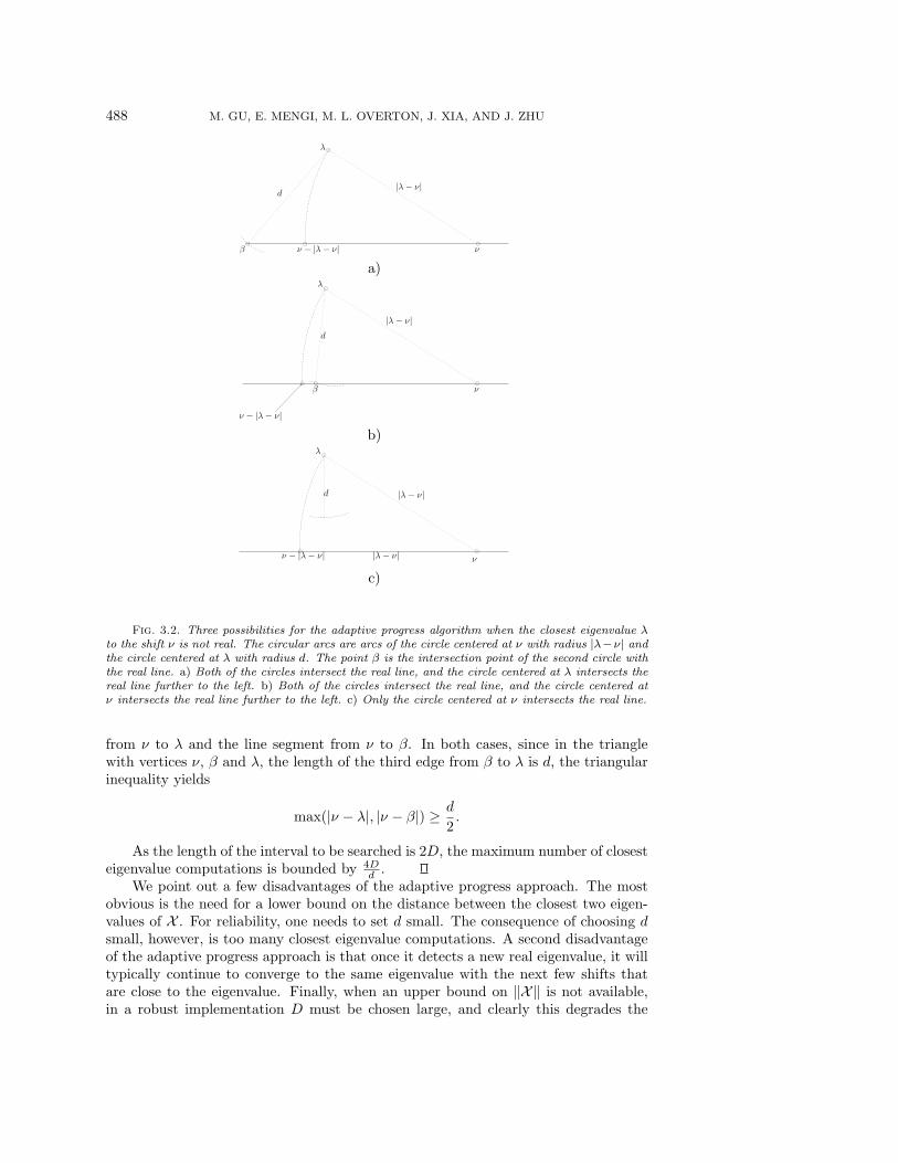
The way the shift ν is updated depends on the closest eigenvalue λ that is found.If λ is real and already discovered, then λ must be larger than ν. In this case thereis no real eigenvalue in the interval (ν − (λ − ν), ν]. Additionally there is no realeigenvalue in the interval (λ − d, λ]. The corresponding update rule in Algorithm 3combines these two conditions. When λ is real and not discovered, the shift ν is λ−d.Finally when the closest eigenvalue is not real, the new shift is set to the leftmost ofthe intersection points of two circles with the real line. One of the circles is centeredat ν and has radius |λ− ν|. The second circle is centered at λ and has radius d.
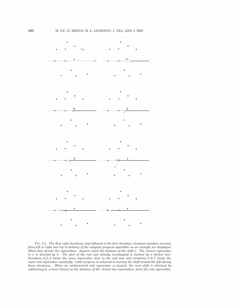
In Figure 3.1 the progress of Algorithm 3 on an example is shown. The algorithmiterates 10 times to investigate the part of the real axis where the eigenvalues areknown to lie. In particular notice that the algorithm locates the same eigenvalue nearthe real axis at the second, third, and fourth iterations and another on the real axisat the fifth, sixth, and seventh iterations. Locating the same eigenvalue a few timesis a deficiency of this algorithm.
486 M. GU, E. MENGI, M. L. OVERTON, J. XIA, AND J. ZHU
λ
νλ
ν
λ
ν
λ
ν
λ
ν
d
λν
λν λ
ν
Fig. 3.1. The first eight iterations (top leftmost is the first iteration; iteration numbers increasefrom left to right and top to bottom) of the adaptive progress algorithm on an example are displayed.Black dots denote the eigenvalues. Squares mark the location of the shift ν. The closest eigenvalueto ν is denoted by λ. The part of the real axis already investigated is marked by a thicker line.Iterations 2, 3, 4 locate the same eigenvalue close to the real axis and iterations 5, 6, 7 locate thesame real eigenvalue repeatedly. Little progress is achieved in moving the shift toward the left duringthese iterations. When an undiscovered real eigenvalue is located, the next shift is obtained bysubtracting d, a lower bound on the distance of the closest two eigenvalues, from the real eigenvalue.
FAST METHODS FOR DISTANCE TO UNCONTROLLABILITY 487
Algorithm 3 Adaptive progress real eigenvalue search algorithm
Call: Λ ← Adaptive Progress(X ,D,d).Input: X ∈ C
q×q, D, an upper bound on the norm of X , and d, a lowerbound for the distance between the closest two eigenvalues ofX .
Output: Λ ∈ Rl with l ≤ q containing all of the real eigenvalues of X
in the interval [−D,D].
1. Initially set the shift ν ← D and the vector of real eigenvalues Λ ← [ ].while ν ≥ −D do
Compute the closest eigenvalue λ to the shift ν.if λ is real then
if λ ∈ Λ then% λ is real and already discovered.ν ← ν − max(|λ− ν|, d− |λ− ν|).
else% λ is real but not discovered yet.Add λ to Λ.ν ← λ− d.
end ifelse
% Otherwise λ is not purely real. Choose the leftmost% intersection point of the circle centered at ν and with% radius |ν − λ| and the circle centered at λ and with% radius d with the real line as the new shift.if d ≥ Im λ then
% Both of the circles intersect the real line.ν ← min(Re λ−
√d2 − Im λ2, ν − |ν − λ|).
else% Only the circle centered at ν intersects the real line.ν ← ν − |ν − λ|.
end ifend if
end while2. Return the real eigenvalue list Λ.
From the description of the algorithm it is not clear whether it terminates. Thenext theorem shows that the adaptive progress algorithm indeed terminates.
Theorem 3.1. Let the shift of Algorithm 3 at a given iteration be ν. The nextshift will be no larger than ν− d
2 . Thus the number of closest eigenvalue computations
is O(Dd ).
Proof. Clearly when the closest eigenvalue λ is real, the shift is decremented byat least d/2. Therefore let us focus on the case when the eigenvalue λ is not real.
We will find a lower bound for the progress h such that the next shift is ν − h.When only the circle centered at ν intersects the real line (i.e., the imaginary part ofλ is greater than d), it is apparent from Figure 3.2c that the distance |λ−ν| is greaterthan or equal to d. Since the next shift is set to the intersection point ν − |λ− ν|, wehave h = |λ−ν| ≥ d. When both of the circles intersect the real line, as in Figure 3.2aand Figure 3.2b, the progress h is the maximum of the lengths of the line segment
488 M. GU, E. MENGI, M. L. OVERTON, J. XIA, AND J. ZHU
λ
β
d|λ − ν|
νν − |λ − ν|
a)λ
d
β
|λ − ν|
ν
ν − |λ − ν|
b)λ
d |λ − ν|
ν|λ − ν|ν − |λ − ν|
c)
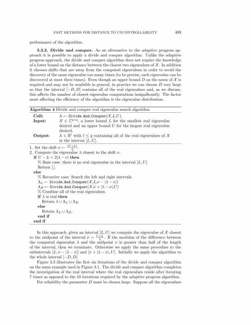
Fig. 3.2. Three possibilities for the adaptive progress algorithm when the closest eigenvalue λto the shift ν is not real. The circular arcs are arcs of the circle centered at ν with radius |λ−ν| andthe circle centered at λ with radius d. The point β is the intersection point of the second circle withthe real line. a) Both of the circles intersect the real line, and the circle centered at λ intersects thereal line further to the left. b) Both of the circles intersect the real line, and the circle centered atν intersects the real line further to the left. c) Only the circle centered at ν intersects the real line.
from ν to λ and the line segment from ν to β. In both cases, since in the trianglewith vertices ν, β and λ, the length of the third edge from β to λ is d, the triangularinequality yields
max(|ν − λ|, |ν − β|) ≥ d
2.
As the length of the interval to be searched is 2D, the maximum number of closesteigenvalue computations is bounded by 4D
d .We point out a few disadvantages of the adaptive progress approach. The most
obvious is the need for a lower bound on the distance between the closest two eigen-values of X . For reliability, one needs to set d small. The consequence of choosing dsmall, however, is too many closest eigenvalue computations. A second disadvantageof the adaptive progress approach is that once it detects a new real eigenvalue, it willtypically continue to converge to the same eigenvalue with the next few shifts thatare close to the eigenvalue. Finally, when an upper bound on ‖X‖ is not available,in a robust implementation D must be chosen large, and clearly this degrades the
FAST METHODS FOR DISTANCE TO UNCONTROLLABILITY 489
performance of the algorithm.
3.3.2. Divide and conquer. As an alternative to the adaptive progress ap-proach it is possible to apply a divide and conquer algorithm. Unlike the adaptiveprogress approach, the divide and conquer algorithm does not require the knowledgeof a lower bound on the distance between the closest two eigenvalues of X . In additionit chooses shifts that are away from the computed eigenvalues in order to avoid thediscovery of the same eigenvalue too many times (to be precise, each eigenvalue can bediscovered at most three times). Even though an upper bound D on the norm of X isrequired and may not be available in general, in practice we can choose D very largeso that the interval [−D,D] contains all of the real eigenvalues and, as we discuss,this affects the number of closest eigenvalue computations insignificantly. The factormost affecting the efficiency of the algorithm is the eigenvalue distribution.
Algorithm 4 Divide and conquer real eigenvalue search algorithm
Call: Λ ← Divide And Conquer(X ,L,U).Input: X ∈ C
q×q, a lower bound L for the smallest real eigenvaluedesired and an upper bound U for the largest real eigenvaluedesired.
Output: Λ ∈ Rl with l ≤ q containing all of the real eigenvalues of X
in the interval [L,U ].
1. Set the shift ν ← (U+L)2 .
2. Compute the eigenvalue λ closest to the shift ν.if U − L < 2|λ− ν| then
% Base case: there is no real eigenvalue in the interval [L,U ].Return [ ].
else% Recursive case: Search the left and right intervals.ΛL ← Divide And Conquer(X ,L,ν − |λ− ν|)ΛR ← Divide And Conquer(X ,ν + |λ− ν|,U)% Combine all of the real eigenvalues.if λ is real then
Return λ ∪ ΛL ∪ ΛR.else
Return ΛL ∪ ΛR.end if
end if
In this approach, given an interval [L,U ] we compute the eigenvalue of X closestto the midpoint of the interval ν = U+L
2 . If the modulus of the difference betweenthe computed eigenvalue λ and the midpoint ν is greater than half of the lengthof the interval, then we terminate. Otherwise we apply the same procedure to thesubintervals [L, ν − |λ − ν|] and [ν + |λ − ν|, U ]. Initially we apply the algorithm tothe whole interval [−D,D].
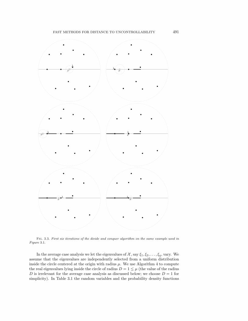
Figure 3.3 illustrates the first six iterations of the divide and conquer algorithmon the same example used in Figure 3.1. The divide and conquer algorithm completesthe investigation of the real interval where the real eigenvalues reside after iterating7 times as opposed to the 10 iterations required by the adaptive progress algorithm.
For reliability the parameter D must be chosen large. Suppose all the eigenvalues
490 M. GU, E. MENGI, M. L. OVERTON, J. XIA, AND J. ZHU
are contained in the disk of radius D′ with D′ D. To discover that there is no realeigenvalue in the interval [D′, D], at most two extra closest eigenvalue computationsare required. If the first shift tried in the interval [D′, D] is closer to D′ than D, thenthe distance from the closest eigenvalue to this shift may be less than half the lengthof the interval [D′, D], so a second closest eigenvalue computation may be needed.Otherwise the interval [D′, D] will be investigated in one iteration. Similar remarkshold for the interval [−D,−D′]. However, the larger choices of D may slightly increaseor decrease the number of shifts required to investigate [−D′, D′]. The importantpoint is that regardless of how large D is compared to the radius of the smallest diskcontaining the eigenvalues, the cost is limited to approximately four extra iterations.
Next we show that the number of closest eigenvalue computations cannot exceed2q + 1 (recall that X ∈ C
q×q).Theorem 3.2 (worst case for Algorithm 4). The number of closest eigenvalue
computations made by Algorithm 3.2 is no more than 2q + 1.Proof. We can represent the progress of the algorithm by a full binary tree,
i.e., a tree with each node having either two children or no children. Each node ofthe tree corresponds to an interval. The root of the tree corresponds to the wholeinterval [−D,D]. At each iteration of the algorithm the interval under considerationis either completely investigated or replaced by two disjoint subintervals that need tobe investigated. In the first case, the node corresponding to the current interval is aleaf. In the second case, the node has two children, one for each of the subintervals.
We claim that the number of leaves in this tree cannot exceed q+1. The intervalscorresponding to the leaves are disjoint. Each such interval has a closest left interval(except the leftmost interval) and a closest right interval (except the rightmost inter-val) represented by two of the leaves in the tree. Each interval is separated from theclosest one on the left by the part of a disk on the real axis in which an eigenvaluelies, and similarly for the closest interval on the right. Since the matrix X has q eigen-values, there can be at most q separating disks and therefore at most q + 1 disjointintervals represented by the leaves of the tree. A full binary tree with q+1 leaves hasq internal nodes. Therefore, the total number of the nodes in the tree, which is thesame as the number of closest eigenvalue computations, cannot exceed 2q + 1.
The upper bound 2q + 1 on the worst case performance of the algorithm is tight,as illustrated by the following example. Consider a matrix with the real eigenvalues2j−1−12j−1 , j = 1, . . . , q, and suppose we search over the interval [−1, 1]. Clearly, the
algorithm discovers each eigenvalue twice except the largest one, which it discoversthree times (assuming that when there are two eigenvalues equally close to a midpoint,the algorithm locates the eigenvalue on the right). Therefore, the total number ofclosest eigenvalue computations is 2q + 1.
Next we aim to show that the average case performance of the algorithm is muchbetter than the worst case. First we note the following elementary result that is animmediate consequence of the fact that the square-root function is strictly concave.
Lemma 3.3. Given l positive distinct integers k1, k2, . . . , kl and l real numbersp1, p2, . . . , pl ∈ (0, 1) such that
∑lj=1 pj = 1, the inequality
√√√√ l∑j=1
pjkj >
l∑j=1
pj√kj(3.19)
holds.
FAST METHODS FOR DISTANCE TO UNCONTROLLABILITY 491
λ
νλ
ν
λν
λν
λν
λν
Fig. 3.3. First six iterations of the divide and conquer algorithm on the same example used inFigure 3.1.
In the average case analysis we let the eigenvalues of X , say ξ1, ξ2, . . . , ξq, vary. Weassume that the eigenvalues are independently selected from a uniform distributioninside the circle centered at the origin with radius μ. We use Algorithm 4 to computethe real eigenvalues lying inside the circle of radius D = 1 ≤ μ (the value of the radiusD is irrelevant for the average case analysis as discussed below; we choose D = 1 forsimplicity). In Table 3.1 the random variables and the probability density functions
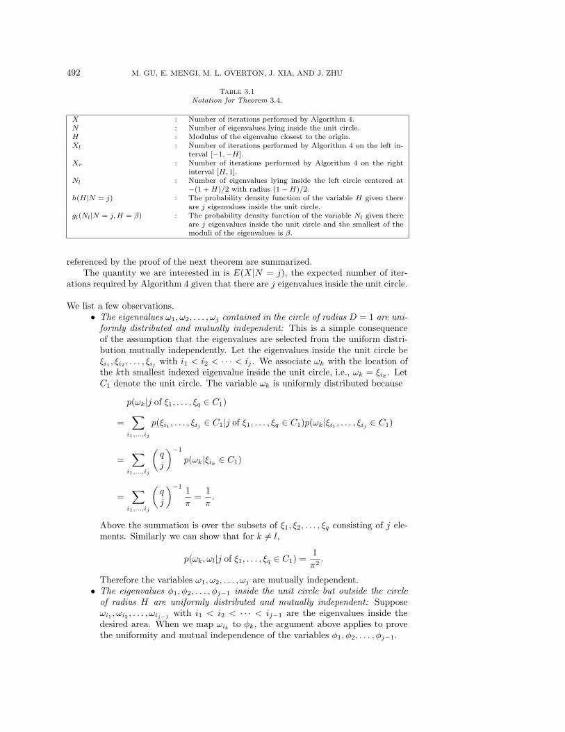
492 M. GU, E. MENGI, M. L. OVERTON, J. XIA, AND J. ZHU
Table 3.1
Notation for Theorem 3.4.
X : Number of iterations performed by Algorithm 4.N : Number of eigenvalues lying inside the unit circle.H : Modulus of the eigenvalue closest to the origin.Xl : Number of iterations performed by Algorithm 4 on the left in-
terval [−1,−H].Xr : Number of iterations performed by Algorithm 4 on the right
interval [H, 1].Nl : Number of eigenvalues lying inside the left circle centered at
−(1 + H)/2 with radius (1 −H)/2.h(H|N = j) : The probability density function of the variable H given there
are j eigenvalues inside the unit circle.gl(Nl|N = j,H = β) : The probability density function of the variable Nl given there
are j eigenvalues inside the unit circle and the smallest of themoduli of the eigenvalues is β.
referenced by the proof of the next theorem are summarized.The quantity we are interested in is E(X|N = j), the expected number of iter-
ations required by Algorithm 4 given that there are j eigenvalues inside the unit circle.
We list a few observations.• The eigenvalues ω1, ω2, . . . , ωj contained in the circle of radius D = 1 are uni-
formly distributed and mutually independent: This is a simple consequenceof the assumption that the eigenvalues are selected from the uniform distri-bution mutually independently. Let the eigenvalues inside the unit circle beξi1 , ξi2 , . . . , ξij with i1 < i2 < · · · < ij . We associate ωk with the location ofthe kth smallest indexed eigenvalue inside the unit circle, i.e., ωk = ξik . LetC1 denote the unit circle. The variable ωk is uniformly distributed because
p(ωk|j of ξ1, . . . , ξq ∈ C1)
=∑
i1,...,ij
p(ξi1 , . . . , ξij ∈ C1|j of ξ1, . . . , ξq ∈ C1)p(ωk|ξi1 , . . . , ξij ∈ C1)
=∑
i1,...,ij
(qj
)−1
p(ωk|ξik ∈ C1)
=∑
i1,...,ij
(qj
)−11
π=
1
π.
Above the summation is over the subsets of ξ1, ξ2, . . . , ξq consisting of j ele-ments. Similarly we can show that for k �= l,
p(ωk, ωl|j of ξ1, . . . , ξq ∈ C1) =1
π2.
Therefore the variables ω1, ω2, . . . , ωj are mutually independent.• The eigenvalues φ1, φ2, . . . , φj−1 inside the unit circle but outside the circle
of radius H are uniformly distributed and mutually independent: Supposeωi1 , ωi2 , . . . , ωij−1 with i1 < i2 < · · · < ij−1 are the eigenvalues inside thedesired area. When we map ωik to φk, the argument above applies to provethe uniformity and mutual independence of the variables φ1, φ2, . . . , φj−1.
FAST METHODS FOR DISTANCE TO UNCONTROLLABILITY 493
• Given c eigenvalues ϑ1, ϑ2, . . . , ϑc inside the left circle with radius 1−H2 cen-
tered at (−(1+H)2 , 0), each eigenvalue is uniformly distributed and mutually
independent: This again follows from the arguments above by mapping φik
to ϑk, where φi1 , φi2 , . . . , φic are the eigenvalues inside the desired region withi1 < i2 < · · · < ic.
• Assuming the number of eigenvalues contained in the circle of radius D isfixed, the expected number of iterations by the algorithm does not depend onthe radius D: Consider the variables ω1 denoting the locations of the j eigen-values all inside the circle of radius D1, and ω2 = D2ω1
D1denoting the locations
of the j eigenvalues inside the circle of radius D2. Let us denote the num-ber of iterations by Algorithm 4 with input ω1 over the interval [−D1, D1] byX1(ω1) and the number of iterations with input ω2 over the interval [−D2, D2]by X2(ω2). It immediately follows that X1(ω1) = X1(
D1ω2
D2) = X2(ω2). By
exploiting this equality we can deduce E(X1|N1 = j) = E(X2|N2 = j),
E(X1|N1 = j) =
∫CD1
X1(ω1)p(ω1) dω1
=
(1
πD21
)j ∫CD1
X1(ω1) dω1
=
(1
πD21
)j ∫CD2
X1
(D1ω2
D2
)D2j
1
D2j2
dω2
=
∫CD2
X2(ω2)p(ω2) dω2
= E(X2|N2 = j),
where N1 and N2 are the number of eigenvalues inside the circle of radiusCD1 of radius D1 and the circle of radius CD2 of radius D2, respectively.Note that the eigenvalues inside both the circle CD1 and the circle CD2 areuniformly distributed and independent, as we discussed above.
By combining these remarks we conclude the equality E(X|N = j) = E(Xl|Nl =j), since the eigenvalues are uniformly distributed and independent inside the circles,and the sizes of the circles do not affect the expected number of iterations given thatthere are j eigenvalues inside the circles.
The next theorem establishes a recurrence equation for E(X|N = j) in terms ofE(X|N = k), k = 0 . . . j − 1. Using the recurrence equation we will show E(X|N =j) = O(
√j) by induction. For convenience let us use the shorthand notation Ej(X)
for E(X|N = j).Theorem 3.4. Suppose the eigenvalues of the input matrices of size q are chosen
from a uniform distribution independently inside the circle of radius μ and Algorithm 4is run over the interval [−1, 1]. The quantity Ej(X) can be characterized by therecurrence equation
E0(X) = 1(3.20)
and for all 0 < j < q
Ej(X) = 2Fj−1(X) + 1,(3.21)
494 M. GU, E. MENGI, M. L. OVERTON, J. XIA, AND J. ZHU
where Fj−1(X) is a linear combination of the expectations E0(X), . . . , Ej−1(X),
Fj−1(X) =
∫ 1
0
(j−1∑k=0
Ek(X)gl(Nl = k|N = j,H = β)
)h(H = β|N = j) dβ.(3.22)
Proof. Equation (3.20) is trivial; when there is no eigenvalue inside the unitcircle, the algorithm will converge to an eigenvalue on or outside the unit circle andterminate.
For j > 0 at the first iteration of the algorithm, we compute the closest eigenvalueto the midpoint and repeat the same procedure with the left interval and with theright interval, so the equality
X = Xl + Xr + 1
and therefore the equality
Ej(X) = E(Xl|N = j) + E(Xr|N = j) + 1(3.23)
follow. Clearly the number of iterations on the left and right intervals depend on themodulus of the computed eigenvalue. By the definition of conditional expectations,we deduce
E(Xl|N = j) =
∫ 1
0
E(Xl|N = j,H = β)h(H = β|N = j) dβ(3.24)
and similarly
E(Xr|N = j) =
∫ 1
0
E(Xr|N = j,H = β)h(H = β|N = j) dβ.(3.25)
Now we focus on the procedures applied on the left and right intervals. Let themodulus of the eigenvalue computed at the first iteration be β. There may be upto j − 1 eigenvalues inside the circle centered at the midpoint of the left interval[−1,−β] and with radius 1−β
2 . The expected number of iterations on the left interval
is independent of the radius 1−β2 and the number of eigenvalues lying outside this
circle. Therefore given the number of eigenvalues inside this circle, by the definitionof conditional expectations, the equality
E(Xl|N = j,H = β) =
j−1∑k=0
E(Xl|Nl = k,N = j,H = β)gl(Nl = k|N = j,H = β)
=
j−1∑k=0
E(Xl|Nl = k)gl(Nl = k|N = j,H = β)
=
j−1∑k=0
Ek(X)gl(Nl = k|N = j,H = β)
(3.26)
is satisfied. A similar argument applies to the right interval to show the analogousequality
E(Xr|N = j,H = β) =
j−1∑k=0
Ek(X)gl(Nl = k|N = j,H = β).(3.27)
FAST METHODS FOR DISTANCE TO UNCONTROLLABILITY 495
By substituting (3.26) into (3.24), (3.27) into (3.25), and combining these with (3.23),we deduce the result.
Corollary 3.5 (average case for Algorithm 4). Suppose the eigenvalues of thematrices input to Algorithm 4 are selected uniformly and independently inside thecircle of radius μ. The expectation Ej(X) is bounded above by c
√j + f − 1 for all
c ≥√
12 and f ∈ [4/c2, 1/3].Proof. The proof is by induction. In the base case, when there is no eigenvalue
inside the unit circle, the algorithm iterates only once, i.e., E0(X) = 1 ≤ c√f − 1.
Assume for all k < j, that the claim Ek(X) ≤ c√k + f − 1 holds. We need
to show the inequality Ej(X) ≤ c√j + f − 1 is satisfied under this assumption. By
definition (3.22) in Theorem 3.4 we have
Fj−1(X) ≤∫ 1
0
(j−1∑k=0
(c√k + f − 1)gl(Nl = k|N = j,H = β)
)h(H = β|N = j) dβ.
(3.28)
As we argued before, the uniformity and independence of each of the j−1 eigenvaluesinside the unit circle but outside the circle of radius H = β is preserved. In otherwords gl(Nl|N = j,H = β) is a binomial density function, and we can explicitly writegl(Nl = k|N = j,H = β), the probability that there are k eigenvalues inside the leftcircle given that there are j − 1 eigenvalues contained in the unit circle and outsidethe circle of radius β, as
gl(Nl = k|N = j,H = β) =
(j − 1k
)(1 − β
4(1 + β)
)k (1 − 1 − β
4(1 + β)
)j−1−k
.
Now the expected value of the binomial distribution above is (j − 1) 1−β4(1+β) . From
Lemma 3.3, we deduce
√j + f
2≥
√j − 1 + 4f
2
≥
√(1 − β)(j − 1)
4(1 + β)+ f
=
√√√√j−1∑k=0
(k + f)gl(Nl = k|N = j,H = β)
>
j−1∑k=0
√k + f gl(Nl = k|N = j,H = β).
Substituting the upper bound√j+f2 for
∑j−1k=0
√k + f gl(Nl = k|N = j,H = β) in
(3.28) yields
Fj−1(X) ≤∫ 1
0
(c√j + f
2− 1
)h(H = β|N = j) dβ =
c√j + f
2− 1.(3.29)
Now it follows from (3.21) that
Ej(X) ≤ c√j + f − 1(3.30)
496 M. GU, E. MENGI, M. L. OVERTON, J. XIA, AND J. ZHU
as desired.
Recall that we intend to apply the divide and conquer approach to A which hassize 2n2×2n2. Assume that the conditions of Corollary 3.5 hold for the eigenvalues ofA and the circle of radius D contains all of the eigenvalues. Suppose also that for anyshift ν, convergence of the shifted inverse iteration or shift-and-invert Arnoldi methodto the closest eigenvalue requires the matrix vector multiplication (A − νI)−1u forvarious u only a constant number of times. Then the average running time of eachtrisection step is O(n4), since finding the closest eigenvalue takes O(n3) time (which isthe cost of solving a Sylvester equation of size 2n a constant number of times) and wecompute the closest eigenvalue O(n) times at each trisection step on average. Becauseof the special structure of the Kronecker product matrix A, even if the input matriceshave eigenvalues uniformly distributed and mutually independent, the eigenvalues ofA may not have this property. However, the numerical examples in the next sectionsuggest that the number of closest eigenvalue computations as a function of the size ofthe Kronecker product matrices is still bounded by O(
√q). According to Theorem 3.2,
in the worst case scenario, each trisection step requires O(n5) operations, which is animprovement over computing all of the eigenvalues of A.
4. Numerical experiments. We first compare the accuracy of the new algo-rithm with the divide and conquer approach, and Gu’s algorithm in [6] on a varietyof examples. Second, we discuss why in general we prefer the divide and conquerapproach over the adaptive progress approach. In our final example we aim to showthe asymptotic running time difference between the new method and Gu’s method.All the tests are run using Matlab 6.5 under Linux on a PC.
4.1. Accuracy of the new algorithm and the old algorithm. We presentresults comparing the accuracy of the new method using the divide and conquer ap-proach with Gu’s method in [6]. In exact arithmetic both the method in [6] and thenew method using the divide and conquer approach must return the same interval,since they perform the same verification by means of different but equivalent eigen-value problems. Our data set consists of pairs (A,B), where A is provided by thesoftware package EigTool [13] and B has entries selected independently from the nor-mal distribution with zero mean and variance one. The data set is available on theweb.3 In all of the tests the initial interval is set [0, σn([A B])] and the trisectionstep is repeated until an interval (l, u] with u− l ≤ 10−4 is obtained.
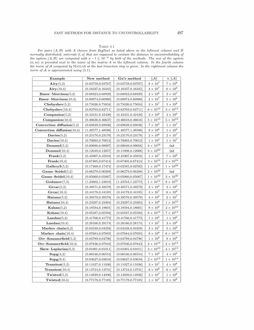
When the second and third columns in Table 4.1 are considered, on most of theexamples the methods return the same interval with the exception of the companion,Demmel, Godunov, and gallery5 examples. The common property of these matricesis that they have extremely ill-conditioned eigenvalues. As we discuss in section 5,when the matrix A has an ill-conditioned eigenvalue, the new method is not expectedto produce accurate small intervals containing the distance to uncontrollability. Onefalse conclusion that one may draw from Table 4.1 is that Gu’s method is alwaysmore accurate than the new method. Indeed for the Basor–Morrison, Grcar, or Lan-dau examples with n = 5 (for which the eigenvalues are fairly well conditioned) thenew method generates more accurate results than Gu’s method when one seeks in-tervals of length around 10−6. In terms of accuracy these two methods have differentweaknesses.
3http://www.cs.nyu.edu/∼mengi/robust stability/data dist uncont.mat.
FAST METHODS FOR DISTANCE TO UNCONTROLLABILITY 497
Table 4.1
For pairs (A,B) with A chosen from EigTool as listed above in the leftmost column and Bnormally distributed, intervals (l, u] that are supposed to contain the distance to uncontrollability ofthe system (A,B) are computed with u − l ≤ 10−4 by both of the methods. The size of the system(n,m) is provided next to the name of the matrix A in the leftmost column. In the fourth columnthe norm of A computed by Matlab at the last trisection step is given. In the rightmost column thenorm of A is approximated using (5.1).
Example New method Gu’s method ‖A‖ ≈ ‖A‖Airy(5,2) (0.03759,0.03767] (0.03759,0.03767] 8 × 10⁷ 7 × 10⁸
Airy(10,4) (0.16337,0.16345] (0.16337,0.16345] 4 × 10⁷ 6 × 10⁸
Basor–Morrison(5,2) (0.68923,0.68929] (0.68923,0.68929] 2 × 10⁶ 2 × 10⁷
Basor–Morrison(10,4) (0.60974,0.60980] (0.60974,0.60980] 2 × 10⁷ 5 × 10⁸
Chebyshev(5,2) (0.75026,0.75034] (0.75026,0.75034] 3 × 10⁷ 5 × 10⁸
Chebyshev(10,4) (0.82703,0.82711] (0.82703,0.82711] 6 × 10¹⁰ 3 × 10¹²
Companion(5,2) (0.42431,0.42438] (0.42431,0.42438] 2 × 10⁸ 4 × 10⁹
Companion(10,4) (0.46630,0.46637] (0.46610,0.46616] 5 × 10¹³ 5 × 10¹⁸
Convection diffusion(5,2) (0.69829,0.69836] (0.69829,0.69836] 7 × 10⁵ 1 × 10⁷
Convection diffusion(10,4) (1.48577,1.48586] (1.48577,1.48586] 9 × 10⁶ 1 × 10⁸
Davies(5,2) (0.23170,0.23176] (0.23170,0.23176] 2 × 10⁶ 2 × 10⁷
Davies(10,4) (0.70003,0.70012] (0.70003,0.70012] 1 × 10⁶ 1 × 10⁷
Demmel(5,2) (0.09090,0.09097] (0.09049,0.09056] 8 × 1049 Inf
Demmel(10,4) (0.12049,0.12057] (0.11998,0.12006] 9 × 1080 Inf
Frank(5,2) (0.45907,0.45916] (0.45907,0.45916] 1 × 10⁷ 7 × 10⁸
Frank(10,4) (0.67405,0.67414] (0.67405,0.67414] 3 × 10¹⁶ 2 × 10¹⁸
Gallery5(5,2) (0.17468,0.17474] (0.02585,0.02592] 1 × 10¹⁶ 1 × 1029
Gauss–Seidel(5,2) (0.06279,0.06288] (0.06279,0.06288] 2 × 10²⁰ Inf
Gauss–Seidel(10,4) (0.05060,0.05067] (0.05060,0.05067] 1 × 1030 3 × 1040
Godunov(7,3) (1.23802,1.23810] (1.23764,1.23773] 1 × 10¹⁴ 8 × 1031
Grcar(5,2) (0.49571,0.49579] (0.49571,0.49579] 2 × 10⁵ 3 × 10⁶
Grcar(10,4) (0.44178,0.44185] (0.44178,0.44185] 4 × 10⁷ 6 × 10⁸
Hatano(5,2) (0.39570,0.39578] (0.39570,0.39578] 4 × 10⁶ 2 × 10⁷
Hatano(10,4) (0.23297,0.23304] (0.23297,0.23304] 4 × 10⁸ 1 × 10¹⁰
Kahan(5,2) (0.18594,0.18601] (0.18594,0.18601] 8 × 10⁸ 2 × 10¹⁰
Kahan(10,4) (0.05587,0.05594] (0.05587,0.05594] 8 × 10¹³ 7 × 10¹⁴
Landau(5,2) (0.41766,0.41773] (0.41766,0.41773] 1 × 10⁵ 1 × 10⁶
Landau(10,4) (0.28166,0.28174] (0.28166,0.28174] 1 × 10⁷ 3 × 10⁸
Markov chain(6,2) (0.04348,0.04358] (0.04348,0.04358] 3 × 10⁷ 5 × 10⁸
Markov chain(10,4) (0.07684,0.07693] (0.07684,0.07693] 8 × 10⁸ 6 × 10¹⁰
Orr–Sommerfield(5,2) (0.04789,0.04796] (0.04789,0.04796] 1 × 10⁹ 8 × 10⁹
Orr–Sommerfield(10,4) (0.07836,0.07843] (0.07836,0.07843] 2 × 10¹⁰ 2 × 10¹²
Skew–Laplacian(8,3) (0.01001,0.01011] (0.01001,0.01011] 3 × 10¹⁰ 4 × 10¹³
Supg(4,2) (0.06546,0.06554] (0.06546,0.06554] 7 × 10⁸ 4 × 10⁹
Supg(9,4) (0.03627,0.03634] (0.03627,0.03634] 2 × 10¹³ 1 × 10¹⁴
Transient(5,2) (0.11027,0.11036] (0.11027,0.11036] 3 × 10⁷ 4 × 10⁸
Transient(10,4) (0.13724,0.13731] (0.13724,0.13731] 6 × 10⁸ 6 × 10⁹
Twisted(5,2) (0.14929,0.14936] (0.14929,0.14936] 2 × 10⁷ 1 × 10⁸
Twisted(10,4) (0.77178,0.77185] (0.77178,0.77185] 1 × 10⁷ 2 × 10⁸
498 M. GU, E. MENGI, M. L. OVERTON, J. XIA, AND J. ZHU
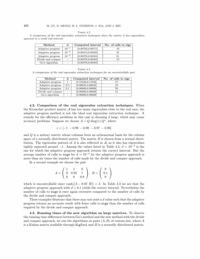
Table 4.2
A comparison of the real eigenvalue extraction techniques when the matrix A has eigenvaluessqueezed in a small real interval.
Method d Computed interval No. of calls to eigs
Adaptive progress 10−1 (0.00702,0.00711] 19
Adaptive progress 10−2 (0.00474,0.00483] 35
Adaptive progress 10−3 (0.00476,0.00484] 81Divide and conquer - (0.00476,0.00484] 13
Gu’s algorithm - (0.00476,0.00484] -
Table 4.3
A comparison of the real eigenvalue extraction techniques for an uncontrollable pair.
Method d Computed interval No. of calls to eigsAdaptive progress 1 (0.13538,0.13546] 17Adaptive progress 0.5 (0.00025,0.00033] 19Adaptive progress 0.1 (0.00000,0.00008] 50
Divide and conquer - (0.00000,0.00008] 12Gu’s algorithm - (0.00000,0.00008] -
4.2. Comparison of the real eigenvalue extraction techniques. Whenthe Kronecker product matrix A has too many eigenvalues close to the real axis, theadaptive progress method is not the ideal real eigenvalue extraction technique. Aremedy for the efficiency problems in this case is choosing d large, which may causeaccuracy problems. Suppose we choose A = Q diag(v) Q∗, where
v = [−1 − 0.99 − 0.98 − 0.97 − 0.96]
and Q is a unitary matrix whose columns form an orthonormal basis for the columnspace of a normally distributed matrix. The matrix B is chosen from a normal distri-bution. The eigenvalue pattern of A is also reflected in A, as it also has eigenvaluestightly squeezed around −1. Among the values listed in Table 4.2, d = 10−3 is theone for which the adaptive progress approach returns the correct interval. But theaverage number of calls to eigs for d = 10−3 by the adaptive progress approach ismore than six times the number of calls made by the divide and conquer approach.
In a second example we choose the pair
A =
⎛⎝ 1 1 0
0 0.95 10 0 0.9
⎞⎠, B =
⎛⎝ 0
0.10
⎞⎠,
which is uncontrollable since rank([A − 0.9I B]) = 2. In Table 4.3 we see that theadaptive progress approach with d = 0.1 yields the correct interval. Nevertheless thenumber of calls to eigs is once again excessive compared to the number of calls bythe divide and conquer approach.
These examples illustrate that there may not exist a d value such that the adaptiveprogress returns an accurate result with fewer calls to eigs than the number of callsrequired by the divide and conquer approach.
4.3. Running times of the new algorithm on large matrices. To observethe running time differences between Gu’s method and the new method with the divideand conquer approach, we run the algorithms on pairs (A,B) of various size, where Ais a Kahan matrix available through EigTool and B is a normally distributed matrix.
FAST METHODS FOR DISTANCE TO UNCONTROLLABILITY 499
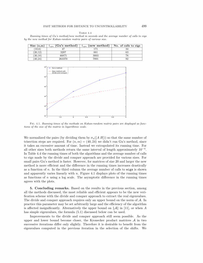
Table 4.4
Running times of Gu’s method/new method in seconds and the average number of calls to eigsby the new method for Kahan-random matrix pairs of various size.
Size (n,m) tcpu (Gu’s method) tcpu (new method) No. of calls to eigs(10,6) 47 171 34(20,12) 3207 881 63(30,18) 46875 3003 78(40,24) 263370 7891 92
1 1.5 2 2.5 3 3.5 410
1
102
103
104
105
106
Gu’s method New method with divide and conquer
Fig. 4.1. Running times of the methods on Kahan-random matrix pairs are displayed as func-tions of the size of the matrix in logarithmic scale.
We normalized the pairs (by dividing them by σn([A B])) so that the same number oftrisection steps are required. For (n,m) = (40, 24) we didn’t run Gu’s method, sinceit takes an excessive amount of time. Instead we extrapolated its running time. Forall other sizes both methods return the same interval of length approximately 10−4.In Table 4.4 the running times of both the algorithms and the average number of callsto eigs made by the divide and conquer approach are provided for various sizes. Forsmall pairs Gu’s method is faster. However, for matrices of size 20 and larger the newmethod is more efficient and the difference in the running times increases drasticallyas a function of n. In the third column the average number of calls to eigs is shownand apparently varies linearly with n. Figure 4.1 displays plots of the running timesas functions of n using a log scale. The asymptotic difference in the running timesagrees with the plots.
5. Concluding remarks. Based on the results in the previous section, amongall the methods discussed, the most reliable and efficient appears to be the new veri-fication scheme with the divide and conquer approach to extract the real eigenvalues.The divide and conquer approach requires only an upper bound on the norm of A. Inpractice this parameter may be set arbitrarily large and the efficiency of the algorithmis affected insignificantly. Alternatively the upper bound on ‖A‖ in [11], or when Ahas simple eigenvalues, the formula (5.1) discussed below can be used.
Improvements to the divide and conquer approach still seem possible. As theupper and lower bound become closer, the Kronecker product matrices A in twosuccessive iterations differ only slightly. Therefore it is desirable to benefit from theeigenvalues computed in the previous iteration in the selection of the shifts. We
500 M. GU, E. MENGI, M. L. OVERTON, J. XIA, AND J. ZHU
address further details of the new algorithm below.
5.1. Sylvester equation solvers. The Sylvester equations needed to performthe multiplication (A−νI)−1u are not sparse in general. We solve them by first reduc-ing the coefficient matrices on the left-hand side of (3.17) to upper quasi-triangularforms (block upper triangular matrices with 1 × 1 and 2 × 2 blocks on the diagonal).Then the algorithm of Bartels and Stewart can be applied [2]. In our implementationwe used the lapack routine dtrsyl [1], which is similar to the method of Bartels andStewart, but rather than computing the solution column by column it generates thesolution row by row, bottom to top. A more efficient alternative may be the recursivealgorithm of Jonsson and Kagstrom [7].
5.2. Difficulties in computing to a high precision. Gu’s method in [6]suffers from the fact that the matrix Q12 in (2.4) becomes highly ill-conditionedas δ → 0 and is not invertible at the limit. This is an issue if the input pair isuncontrollable or nearly uncontrollable.
For the new method instability is caused by small η. The accuracy of the algo-rithm depends on the ability to extract the real eigenvalues of A successfully. (Theimaginary eigenvalues of H(α) can be obtained reliably by using a Hamiltonian eigen-value solver.) A computed eigenvalue of A differs from the exact one by a quantitywith modulus on the order of ‖A‖εmach/|w∗z|, where w and z are the correspondingunit left and right eigenvectors, respectively. In general the more dominant factor inthe formation of this numerical error is the norm ‖A‖ rather than the absolute con-dition number of the eigenvalue (appearing in the denominator), since the invertedmatrix in the definition of A is the inverse of a matrix that is nearly singular for smallη, and therefore the norm of A is big. There is another numerical trouble caused bybig ‖A‖. We cannot expect to solve the linear system (A − νI)x = u accurately forA with large norm. This obviously has an effect on the convergence of shifted inverseiteration and shift-and-invert preconditioned Arnoldi especially considering the factthat the shift ν is not close to an eigenvalue in general. (Because of this, computingthe eigenvalues of A using the QR algorithm may be superior to computing themusing shifted inverse iteration or shift-and-invert preconditioned Arnoldi, as indeedwe observed in practice.) In our experience eigs has convergence problems typicallywhen the norm of A reaches the order of 1010. Smaller η contributes to the increasein the norm of A; however, it is not the only factor. Indeed for certain pairs (A,B)the norm ‖A‖ is large even when η is not small. Under the assumption that A isdiagonalizable, an upper bound on ‖A‖ is derived in [11]. Specifically when A hassimple eigenvalues, the upper bound on ‖A‖ in [11] simplifies to
2‖A‖ +(2‖BB∗/δ − δI‖ + δ)2
η infdet(A−λI)=0 |y∗λxλ|2(5.1)
with xλ and yλ denoting the unit right and unit left eigenvectors, respectively, cor-responding to λ. Notice that the upper bound given by (5.1) can be efficiently com-puted in O(n3) time, and therefore in an implementation it can be used to estimatethe length of the smallest interval containing the distance to uncontrollability thatcan possibly be computed accurately. Surprisingly the norm of A heavily depends onthe worst conditioned eigenvalue of A, but it has little to do with the norm of A. Forinstance, when A is normal and ‖B‖ is not very large, we expect that ‖A‖ exceeds1010 only when η is smaller than 10−10 unless the pair (A,B) is nearly uncontrollable.This in turn means we can reliably compute an interval of length 10−10 containing
FAST METHODS FOR DISTANCE TO UNCONTROLLABILITY 501
the distance to uncontrollability. On the other hand when A is far from being normalor the pair (A,B) is close to being uncontrollable and a small interval is required, thenew method performs poorly. The accuracy of the intervals generated on various ex-amples in Table 4.1 in the second column is also justified by (5.1). All of the examplesfor which the method performs poorly are highly nonnormal. In the fourth column inTable 4.1 the norms of A computed by calling Matlab’s norm at the last trisectionstep (approximately when η is the difference between the upper and lower bounds ofthe interval in the second column and δ is the upper bound of the interval) are listed.In the rightmost column the upper bounds on the norm of A using (5.1) are provided.For most of the pairs in Table 4.1 the upper bound on ‖A‖ in the rightmost columnis tight.
5.3. Alternative eigenvalue problem. To see whether there exists an α suchthat H(α) and H(α + η) share an eigenvalue, we extract the real eigenvalues of A.Alternatively we can solve the generalized eigenvalue problem
P − λM =
⎛⎜⎜⎝
−A∗1 −AT
2 δI δI 0BT
2 −A∗1 + A2 0 δI
B1 0 A1 −AT2 δI
0 B1 BT2 A1 + A2
⎞⎟⎟⎠− λ
⎛⎜⎜⎝
−I 0 0 00 0 0 00 0 0 00 0 0 I
⎞⎟⎟⎠.
(5.2)
The real eigenvalue extraction techniques are applicable to this problem as well, sincethe scalar λ is an eigenvalue of the pencil above if and only if 1
λ−ν is an eigenvalue of
the matrix (P −νM)−1M . The multiplication x = (P −νM)−1My can be performedefficiently by solving the linear system (P − νM)x = My. When we write this linearsystem in matrix form, we obtain the Sylvester equation (3.3) but with α replaced byν and with the matrix (
−Y11 00 Y22
)
replacing 0 on the right-hand side, where y = [vec(Y11) y12 y21 vec(Y22)]T with
equal sized block components. Notice that the fact that the eigenvalue problem (5.2)is of double size compared to the eigenvalue problem Ax = λx is not an efficiencyconcern. We still solve Sylvester equations of the same size. The real issue is thatthese two eigenvalue problems have different conditioning. Theoretically either ofthem can be better conditioned than the other in certain situations. In practice weretrieved more accurate results with the eigenvalue problem Ax = λx most of thetime, even though there are also examples on which the algorithm using (5.2) yieldsmore accurate results.
6. Software. By combining the new verification scheme and BFGS, it is possibleto come up with a more efficient and accurate algorithm. A local minimum of thefunction σn([A − λI B]) can be found in a cheap manner by means of the BFGSoptimization algorithm. Notice that the cost of this local optimization step is O(1),since we are searching over two unknowns, namely, the real and the imaginary partsof λ. Using the new verification scheme we can check whether the local minimum isindeed a global minimum as described in [3, Algorithm 5.3]. If the local minimumis not a global minimum, the new verification scheme also provides us with a pointλ′, where the value of the function σn([A − λI B]) is less than the local minimum.
502 M. GU, E. MENGI, M. L. OVERTON, J. XIA, AND J. ZHU
Therefore we can repeat the application of BFGS followed by the new scheme untilwe verify that the local minimum is a global minimum.
An efficient implementation of the new method is freely available.4 In this im-plementation, by setting an input parameter appropriately, one can either run thetrisection method or the hybrid method just described. Typically, the new scheme isfaster than the previous implementation of the trisection method of [3] for matricesof size larger than 20.
Acknowledgements. Many thanks to A. Yılmaz for carefully reading the aver-age case analysis for the divide and conquer approach. We are also grateful to twoanonymous referees for their invaluable suggestions.
REFERENCES
[1] E. Anderson, Z. Bai, C. Bischof, S. Blackford, J. Demmel, J. Dongarra, J. Du Croz,
A. Greenbaum, S. Hammarling, A. McKenney, and D. Sorenson, LAPACK Users’Guide, 3rd ed., SIAM, Philadelphia, 1999.
[2] R. H. Bartels and G. W. Stewart, Solution of the equation AX + XB = C, Comm. ACM,15 (1972), pp. 820–826.
[3] J. V. Burke, A. S. Lewis, and M. L. Overton, Pseudospectral components and the distanceto uncontrollability, SIAM J. Matrix Anal. Appl., 26 (2004), pp. 350–361.
[4] R. Eising, The distance between a system and the set of uncontrollable systems, in Mathe-matical theory of networks and systems, Lecture Notes in Control and Inform. Sci., 58,Springer, London, 1984, pp. 303–314.
[5] R. Eising, Between controllable and uncontrollable, System Control Lett., 4 (1984), pp. 263–264.
[6] M. Gu, New methods for estimating the distance to uncontrollability, SIAM J. Matrix Anal.Appl., 21 (2000), pp. 989–1003.
[7] I. Jonsson and B. Kagstrom, Recursive blocked algorithm for solving triangular systems,Part I: One-sided and coupled Sylvester-type matrix equations, ACM Trans. Math. Soft-ware, 28 (2002), pp. 392–415.
[8] R. E. Kalman, Mathematical description of linear dynamical systems, J. SIAM Control Ser.A, 1 (1963), pp. 152–192.
[9] R. B. Lehoucq, K. Maschoff, D. Sorensen, and C. Yang, ARPACK Software Package,http://www.caam.rice.edu/software/ARPACK/, 1996.
[10] R. B. Lehoucq, D. Sorensen, and C. Yang, ARPACK Users’ Guide, SIAM, Philadelphia,1998.
[11] E. Mengi, Measures for Robust Stability and Controllability, Ph.D. thesis, Courant Instituteof Mathematical Sciences, New York, NY, 2006.
[12] C. C. Paige, Properties of numerical algorithms relating to computing controllability, IEEETrans. Automat. Control, 26 (1981), pp. 130–138.
[13] T. G. Wright, EigTool: A graphical tool for nonsymmetric eigenproblems, Oxford Uni-versity Computing Laboratory, Oxford, UK, http://www.comlab.ox.ac.uk/pseudospectra/eigtool/, 2002.
4http://www.cs.nyu.edu/∼mengi/robust stability/dist uncont.html.