KATHOLIEKE UNIVERSITEIT

LEUVEN

OEPARTEMENT TOEGEPASTE ECONOMISCHE WETENSCHAPPEN

RESEARCH REPORT 0224

THE MULTIVARIATE LEAST TRIMMED SQUARES ESTIMATOR

by J. AGULLO C.CROUX

S. VAN AELST

0/2002/2376/24

The Multivariate Least Trimmed Squares Estimator

Jose Agu1l61, Christophe Croux,2 and Stefan Van Aelst,3

Abstract

In this paper we introduce the least trimmed squares estimator for multivariate

regression. We give three equivalent formulations of the estimator and obtain its

breakdown point. A fast algorithm for its computation is proposed. We prove Fisher­

consistency at the multivariate regression model with elliptically symmetric error dis­

tribution and derive the influence function. Simulations investigate the finite-sample

efficiency and robustness of the estimator. To increase the efficiency of the estimator,

we also consider a one-step reweighted version, as well as multivariate generalizations

of one-step GM-estimators.

Keywords: Multivariate Regression, Breakdown Point, Generalized M-estimator, Influence

Function, Minimum Covariance Determinant Estimator.

1 Introduction

Consider the multivariate regression model

i = 1, ... ,n with Xi = (Xil"",Xip)t E IRP and Yi = (Yil"",Yiq)t E IRq. The matrix

BE IRpxq contains the regression coefficients. The error terms El, .. , , En are i.i.d. with zero

center and as scatter a positive definite and symmetric matrix 2: of size q. Furthermore,

we assume that the errors are independent of the carriers. Note that this model generalizes

both the univariate regression model (q = 1) and the multivariate location model (Xi = 1).

Denote the entire sample Zn = {(Xi,Yi);i = 1, ... ,n} and write X = (Xl, ... ,Xn)t for the

1 Departamento de Fundamentos del An81isis Economico, University of Alicante, E-03080, Alicante, Spain 2Dept. of Applied Economics, KULeuven, Naamsestraat 69, B-3000 Leuven, Belgium. 3Dept. of Applied Mathematics and Computer Science, Ghent University, Krijgslaan 281 S9, B-9000

Gent, Belgium.

1

design matrix and Y = (Yl, ... , Yn)t for the matrix of responses. The classical estimator for

B is the least-squares (LS) estimator BLS which is given by

while ~ is unbiasedly estimated by

• 1 • t • ~LS = --(Y - XBLS ) (Y - XBLS).

n-p

(1.1)

(1.2)

Since the least squares estimator is extremely sensitive to outliers, we aim to construct a ro­

bust alternative. An overview of strategies to robustify the multivariate regression method

is given by Maronna and Yohai (1997) in the context of simultaneous equations models.

Koenker and Portnoy (1990) apply a regression M-estimator to each coordinate of the re­

sponses and Bai et al. (1990) minimize the sum of the euclidean norm of the residuals.

However, these two methods are not affine equivariant. Methods based on robust estima­

tion of the location and scatter of the joint distribution of the (x, y) variables have been

introduced by Ollila et al. (2001,2002) who use rank and sign based covariance matrices

and by Rousseeuw et al. (2000) who use the Minimum Covariance Determinant estimator

(Rousseeuw 1984). Our approach will be different from the latter, since it will be based

on the covariance matrix of the residuals, more than on the covariance matrix of the joint

distribution.

In Section 2 we give a formal definition of the multivariate least trimmed squares (MLTS)

estimator and derive two equivalent formulations allowing us to study more easily the prop­

erties of the estimator. In Section 3 we show that the estimator has a positive breakdown

point (BDP). A time efficient algorithm to compute the MLTS is presented in Section 4. In

Section 5 we give a functional version of the multivariate least trimmed squares estimator

and show that the estimator is Fisher-consistent at the multivariate regression model with

elliptically symmetric error distribution. Afterwards, in section 6 we derive its influence

function and compute asymptotic variances and corresponding efficiencies. In section 7 we

consider a one-step reweighted version of the estimator as well as a multivariate generaliza­

tion of one-step GM estimators with Mallows and Schweppe type weights using the MLTS

as initial estimator. Section 8 presents simulation results. Simulations have been done to

investigate the finite-sample efficiency and robustness of the MLTS estimator. Section 9

presents a real data example while Section 10 concludes. The Appendix contains all the

proofs.

2

2 Definition and properties

Our approach consists of finding the subset of h observations having the property that the

determinant of the covariance matrix of its residuals from a LS-fit solely based on this subset

is minimal. The resulting estimator will then be simply the LS-estimator computed from

the optimal subset. The definition of the estimator is reminiscent of that of the MCD

location/scatter estimator of Rousseeuw (1984), and reduces to it in case of a multivariate

regression model with only an intercept, where X = (1, ... , 1Y E /Rn . Indeed in the latter

case the multivariate regression model reduces to a multivariate location model. We will

show that our approach is equivalent to the selection of the value of B which minimizes the

determinant of the robust MCD scatter matrix of the residuals. Of course, one could also

think of minimizing the determinant of other robust covariance matrices of the residuals. As

such, Bilodeau and Duchesne (2000) used S-estimators as robust estimator of the covariance

of the residuals in the context of seemingly unrelated regression. We thus use the Minimum

Covariance Determinant estimator (MCD) as scatter matrix estimator of the residuals. The

main reason for this choice is that it turns out to be easy to develop a fast algorithm for

the resulting multivariate regression estimator. Moreover, the resulting estimator has a high

BDP and is ideally suited as initial estimator for one (or more) step procedures.

Consider a dataset Zn = {(Xi, Yi); i = 1, ... , n} C IRp+q and for any B E IRpxq denote

ri(B) = Yi - BtXi the corresponding residuals. Let 1{ = {H c {I, ... ,n}I#H = h} be the

collection of all subsets of size h. For any H E 1{ denote BLS(H) the least squares fit based

solely on the observations {(Xj,Yj);j E H}. Furthermore, for any H E 1{ and B E /Rpxq

denote cov(H,B) := k 2:jEH(rj(B) - TH(B))h(B) - TH(B))t, with TH(B) := k 2:jEH rj(B),

the covariance matrix of the residuals with respect to the fit B, belonging to the subset H.

Then the MLTS estimator is defined as follows:

Definition 1. With the notations above the multivariate least trimmed squares estimator

(MLTS) is defined as

BMLTS(Zn) = BLS(if) where if E argmin det tLs(H) HE1/.

(2.1)

with tLs(H) = cov(H, BLS(H)) for any H E 1{. The covariance of the errors can then be

estimated by

(2.2)

where e", is a consistency factor.

3

Note that if the minimization problem has more than one solution, in which case we look

at argminH det 'f:.Ls(H) as a set, we arbitrarily select one of these solutions to determine

the MLTS estimator. In Section 5 a consistency factor c'" will be proposed to attain Fisher­

consistency at the specified model. Note that for h = n we find back the classical least

squares estimator. Throughout the text we will suppose that the dataset Zn = {(Xi, Yi); i =

1, ... , n} C IRp+q is in general position in the sense that no h points of Zn are lying on the

same hyperplane of IRp+q. Formally, this means that for all f3 E IRP, 'Y E IRq, it holds that

(2.3)

unless if f3 and 'Yare both zero vectors. For datasets in general position we will now give

two equivalent characterizations of the MLTS estimator. First, we need the following lemma

which is a generalization of the characterization of Grubel (1988) of the mean and covariance

matrix of a multivariate distribution.

Lemma 1. Let z = (x, y) be a (p + q)-dimensional random variable having distribution K.

Suppose that EK[XXt] is a strictly positive definite matrix. Define BLS(K) = EK[xxt]-l EK[xyt]

and L:Ls(K) = Cova(c) := EK[cct] where c := y - (BLS(K))lx. Then among all pairs (b,6.)

with b E IRpxq and 6. a positive definite and symmetric matrix of size q such that

(2.4)

the unique pair which minimizes det6. is given by (BLS(K), L:Ls(K)).

Note that if not all points of a dataset are lying in a subspace of IRp+q, then Lemma 1

can be applied by taking for K the empirical distribution function associated to the data.

This results in a characterization of the sample least squares estimators for the multivariate

regression model.

Now we are ready to show that the MLTS estimator can also be obtained as the B

minimizing the determinant of the M CD scatter matrix estimate computed from its residuals.

Herefore, denote MCDq(B) the MCD-scatter matrix based on the residuals from B. Formally,

with iI E argmindet Cova(H, B) for any H E 1i and B E IRpxq. The residual covariance HE1i

matrices we consider are thus centered at zero. (If we work with a model with intercept it

can be shown that "Cova" may be replaced by the usual sample covariance matrix of the

residuals. )

4

Proposition 1. With the notations above, for datasets in general position, we have that

argmin det MCDq(B) = {r3Ls(iI) IiI E argmin det tLs(H)} (2.5) 13 HEH

Proposition 1 shows that any B which minimizes the determinant of the MCD scatter es­

timate of its residuals is also a solution of (2.1). In the case of unique solutions, which we

have almost surely if we sample from a continuous distribution, we can rewrite (2.5) as

r3MLTS (Zn) = argmin det MCDq(B). 13

For the residual scatter estimator we have

(2.6)

(2.7)

A third characterization of the MLTS is based on the distances of the residuals. For any

BE mpxq and 2: E PDS(g), the set of positive definite and symmetric matrices of size g, we

define the squared distances (for the 2: metric) of the residuals w.r.t. Bas

Denote d1:n(B,2:) ::; ... ::; dn:n(B,2:) the ordered sequence of distances of the residuals.

Then the MLTS estimator can also be obtained in the following way.

Proposition 2. Consider h

argmin l:>;:n(B, 2:) 13,2:;12:1=1 j=1

where the minimum is over all B E mpxq and 2: E PDS(g) with det 2:

12:1 = 1). Then for datasets in general position it holds that

(2.8)

1 (denoted as

{ r3 l(r3, f;) E argmin t d;:n(B, 2:)} = {r3Ls(iI) IiI E argmin det tLs(H)} (2.9) 13,2:;12:1=1 j=1 H

Proposition 2 shows that any 13 minimizing the sum of the h smallest squared distances of its

residuals (subject to det 2: = 1) is also a solution of (2.1). For any (13, f;) that minimizes (2.8)

denote iI := {j; d;(r3, f;) ::; d~:n(r3, f;)} E 7t the set of indices corresponding to the h smallest

squared distances of the residuals. In the case of unique solutions, Proposition 2 yields

h

r3MLTS (Zn) = argmin L d}n(B, 2:), 13,2:;12:1=1 j=1

5

(2.10)

so the MLTS estimator minimizes the sum of the h smallest squared distances of its resid­

uals (subject to the condition det2: = 1). Note that in the case q = 1 expression (2.8)

reduces to argmins 2:7=1 rJ,n(B) , with r1:n(B) :::; ... :::; rn:n(B) the ordered residuals w.r.t.

B. Hence in the case of univariate regression our estimator minimizes the sum of the h small­

est squared residuals, and thus corresponds to the Least Trimmed Squares estimator (LTS)

of (Rousseeuw 1984). This explains why we call our estimator the MLTS estimator. The

LTS is a well-known positive-breakdown robust estimator for regression which is frequently

used.

3 Breakdown point

To study the global robustness of the MLTS estimator we compute its finite-sample break­

down point. The finite-sample breakdown point c~ of an estimator Tn is the smallest fraction

of observations from Zn that need to be replaced by arbitrary values to carry the estimate

beyond all bounds (Donoho and Huber 1983). Formally, it is defined as

where the supremum is over all possible collections Z~ obtained from Zn by replacing m data

points by arbitrary values. For any dataset Zn C mp+q denote k(Zn) the maximal number

of observations of Zn lying on a same hyperplane of mp+q . Since we required that Zn is in

general position, we have k(Zn) < h. We now have the following theorem.

Theorem 1. For any dataset Zn C mp+q in general position with q > 1 it holds that

*(8 Z)_min(n-h+1,h-k(Zn)) Cn MLTS, n - n . (3.1)

It follows that if we take h = "In for some fraction 0 < "I :::; 1 then the corresponding

breakdown point equals C~(8MLTS, Zn) = min(l - "I + l/n, "I - k(Zn)/n). If the dataset Zn

comes from a continuous distribution F, then with probability 1, no p + q points belong

to the same hyperplane of mp+q . This implies k(Zn) = p + q - 1 and f~(8MLTS' Zn) =

min(n - h + 1, h - p - q + l)/n almost surely. Then for h = "In the breakdown point of

the MLTS tends to min(l - "1,"1). It follows that for data with k(Zn) = p + q - 1 any

choice [(n + p + q)/2] :::; h :::; [(n + p + q + 1)/2] yields the maximal breakdown point

([(n - p - q)/2] + l)/n ~ 50%.

6

Remark: In the case q = 1 the proof of Theorem 1 becomes much easier and yields the

following result for the breakdown point of the LTS estimator.

Corollary 1. Denote k'(Zn) the maximal number ofxj E {x;;i = 1, ... ,n} lying on a

hyperplane of IR? Then for any dataset Zn C IR?+I with k'(Zn) < h it holds that

*(8' Z) _ min(n-h+l,h-k'(Zn)) En LTS, n - .

n (3.2)

If Zn comes from a continuous distribution F then almost surely k'(Zn) = P - 1 yielding

E~(8LTS, Zn) = min(n - h + 1, h - p + 1)/n, as was already obtained by Hiissjer (1994). In

this case any [(n + p)/2] ::; h ::; [(n + p + 1)/2] gives the maximal breakdown point.

4 Algorithm

Recently, Rousseeuw and Van Driessen (1999) developed a fast algorithm to compute the

MCD location and scatter estimator. The basic tool for this algorithm was the so called

C-step which guaranteed to decrease the MCD objective function. Similarly, the following

theorem gives a C-step which can only decrease the MLTS objective function.

Theorem 2. Take HI E H with corresponding least squares estimates 81 := 8 Ls(Hr) and

tl := tLs(HI). If det(t I ) > 0 then denote by H2 the set of indices of the observations

corresponding with the h smallest residual distances dI :n (8I ,tI ) ::; ... ::; dh :n(8 I,tr). For

82 := 8 Ls (H2) and t2 := t Ls (H2), we have

with equality if and only if 82 = 81 and t2 = t l.

Constructing in this way from HI a new subsample H2 is called a C-step where, following

Rousseeuw and Van Driessen (1999), C stands for "concentration" because the new subsam­

pIe H2 is more concentrated than HI in the sense that det(t2 ) is lower than det(t I ).

The C-step of Theorem 2 forms the basis of our MLTS algorithm we will describe now. We

start by drawing m random p + q subsets Jm of {I, ... , n} and compute the corresponding

least squares estimators 8m := 8 Ls (Jm ) and tm := tLS(Jm ). If det(tm) = 0 for some

subset Jm then we draw additional points until det(tm ) > 0 or #Jm = h. For each subset

we compute the residual distances d;(8m , t m ) for i = 1, ... , n and denote HI the subset

corresponding to the h observations with smallest residual distances. Then we apply some

7

C-steps (e.g. two), lowering each time the value of the objective function. We then select

the 10 subsets Jm which yielded the lowest determinants and for them we carry out further

C-steps until convergence. The resulting subsample with lowest determinant among the 10

will be the final solution reported by the algorithm. For large datasets the algorithm can be

speed up by using nested extensions as proposed by Rousseeuw and Van Driessen (1999).

5 The Functional

The functional form of the MLTS estimator can be defined as follows. Let K be an arbitrary

(p + q) dimensional distribution which represents the joint distribution of the carriers and

response variables. Denote by 0 < a < 1 the mass not determining the MLTS estimator and

define

VIda) = {AI A c lRp +q measurable and bounded with PK(A) = 1 - a}. (5.1)

To define the MLTS estimator at the distribution K we require that

h((3tx = 0) < 1 - a for all (3 E mp \ {O}.

For each A E VK(a), the least squares solution over the set A is then given by

and EA(K) = JA(Y - BA(K)tx)(y - BA(K)tx)t dK(x, y).

1-a

(5.2)

(5.3)

(5.4)

Furthermore, a set A E VK(a) is called an MLTS solution if det(EA(K» ::; det(EA(K» for

any other A E VK(a). The MLTS functionals at the distribution K are then defined as

BMLTS(K) = BA(K) and EMLTS(K) = cnEA(K). (5.5)

The constant en can be chosen such that consistency will be obtained at the specified model.

If the distribution K is not continuous, then the definition of 'DK(a) can be modified as in

Croux and Haesbroeck (1999) to ensure that the set VK(a) is non-empty.

Now consider the multivariate regression model

8

where x = (Xl' ... ' Xp) is the p-dimensional vector of explanatory variables, Y = (Yl, ... , Yq)

is the q-dimensional vector of response variables and E: is the error term. We suppose that E:

is independent of X and has a distribution FE with density

where 2:: E PDS(q). The function g is assumed to have a strictly negative derivative g' such

that FE is a unimodal elliptically symmetric distribution around the origin. The distribution

of z = (x, y) is denoted by H. A regularity condition (to avoid degenerate situations) on the

model distribution H is that

(5.6)

for all (3 E IRP and I E IRq not both equal to zero at the same time. If a = 0 this regularity

condition means that the distribution H is not completely concentrated on a (p + q - 1)­

dimensional hyperplane. If a > 0 this general position condition says that the maximal

amount of probability mass of H lying on the same hyperplane must be lower than 1 - a.

We first give the following proposition which says that the MLTS solution can always be

taken as a cylinder.

Lemma 2. Consider a distribution H satisfying (5.6) and an MLTS solution A E DH(a).

For any (x, y) E IRp+q denote d2 (x, y) = (y-B A(H)tx)t(2::;JH))-1 (y- B A(H)tx). Define the

cylinder [; = {(x, y) E IRp+q; d2 (x, y) ::::; D~} where D~ is chosen such that PH([;) = 1 - a.

Then it holds that

We now show that the functionals BMLTS(H) and 2::MLTS(H) defined by (5.5) for some

well chosen constant c'" are Fisher-consistent for the parameters Band 2::.

Theorem 3. Denote I-a

c'" = ~luIl2:sqQ uI dFo(u)

where Fo = FIq is the central error distribution and q", = K-I(I-a) with K(t) = Ppo(UtU ::::;

t). Then the functionals BMLTS and 2::MLTS are Fisher-consistent estimators for the param­

eters Band 2:: at the model distribution H:

9

Note that for obtaining the above consistency result we only made an assumption on the

distribution of the errors, but not on the distribution of (x, y). For multivariate normal

errors we can take c'" = (1 - ex)/ Fx2 (q",) with q", = Xp2 1-"" the upper ex percent point of p+2 I

the X~ distribution.

6 The influence function and asymptotic variances

The influence function of a functional T at the distribution H measures the effect on T of

adding a small mass at z = (x, y). If we denote the point mass at z by .6.. and consider the

contaminated distribution He,. = (1 - c)H + c.6.. then the influence function is given by

fP( . T H) - r T(He,z) - T(H) - !i...T(H ) z" - ~W c - Be: e,. le=o'

(See Hampel et al. 1986.) It can easily be seen that the MLTS is equivariant for affine

transformations of the regressors and responses and for regression transformations which

add a linear function of the explanatory variables to the responses. Therefore, it suffices

to derive the influence function at a model distribution Ho for which B = 0 and the error

distribution Fo = Fl. with density fo(Y) = g(yty ). The following theorem gives the influence

function of the MLTS regression functional at Ho.

Theorem 4. With the notations from above, we have that

where C2 is given by

IF(z; BMLTS , Ho) = EHo [xxtrl x2yt f(lIyIl2::; q",)

- C2

7rq/ 2 1..jq; C2 = rq+1g'(r2) dr

r(q/2 + 1) 0

(6.1)

Note that the influence function is bounded in y but unbounded in x. Closer inspection

of (6.1) shows, however, that only good leverage points, which have outlying x but satisfy

the regression model, can have a high effect on the MLTS estimator. Bad leverage points

will give a zero influence. In the case of simple regression, the influence function of the LTS

slope has been plotted in Croux et al. (1994, Figure 3d).

Remark 1,' The influence function of the MCD location estimator Tq at a q-dimensional

spherical distribution Fo can be obtained from Butler, Davies and Jhun (1993) or Croux and

Haesbroeck (1999). With the notations as before it is given by

10

Therefore, it follows that the influence function of BMLTS can be rewritten as

(6.2)

Remark 2: In the case q = 1 we have C2 = J~g'(y2)y2dy = y7i;f(y7i;) - ((1- 0:)/2) so

we obtain

( t -1 xyI(y2 ::; qa) IF Zj BlvILTS, Ho) = EHo[xx] 1 _ 0: _ 2y7i;f( y7i;)

which is the expression for the influence function of the LTS estimator.

Remark 3: Similarly as in Theorem 4 it can be shown that

IF(Zj EMLTS , Ha) = IF(y, Cq, Fo)

where Cq is the q-dimensional MCD scatter estimator. The influence function of the MCD

scatter estimator at elliptical distributions can be obtained from Croux and Haesbroeck

(1999).

The asymptotic variance-covariance matrix of BMLTS can now be computed by means

of ASV(BMLTS , Ho) = EH[IF(zj BMLTS , Ho) @ IF(zj BMLTS , Ho)t] (see e.g. Hampel et al.

1986). Here A 0 E denotes the Kronecker product of a (d1 x d2) matrix A with a (d3 x d4 )

matrix E, which results in a (d1d3 x d2d4 ) matrix with d1d2 blocks of size (d3 x d4 ). For

1::; j ::; d1 and 1 ::; k ::; d2 the (j, k)-th block equals ajkE, where ajk are the elements of the

matrix A. Let us denote Ex ;= EHo [xxt], then expression (6.2) implies that

(6.3)

where the commutation matrix Dp,q is a (pq x pq) matrix consisting of pq blocks of size

(q x pl. For 1 ::; l ::; p and 1 ::; m ::; q the (l,m)th block of Dp,q equals the (q x p) matrix

/:::"ml which is 1 at entry (m, l) and 0 everywhere else.

From (6.3) it follows that for every 1 ::; i ::; p and 1 ::; j ::; q the asymptotic covariance

matrix of (BMLTS)ij is given by /:::"jiE;1 ASV((Tq)j, Fo)) which implies that the asymptotic

variance of (B M LTS )ij equals

For i =I i' we obtain the asymptotic covariances

EH[IF(Zj (BMLTS)ij, Ho)IF(zj (BMLTS)i'j, Ho)]

(E;l)ii,ASV((Tq)j, Fo)

11

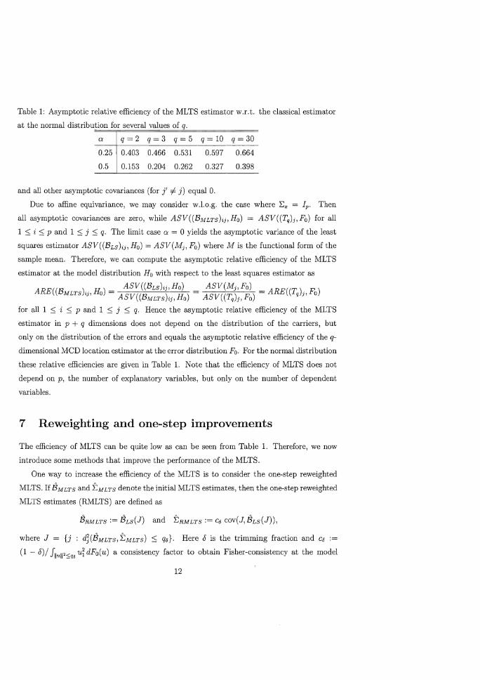
Table 1: Asymptotic relative efficiency of the MLTS estimator w.r.t. the classical estimator

at the normal distribution for several values of q.

a q=2 q=3 q=5 q= 10 q= 30

0.25 0.403 0.466 0.531 0.597 0.664

0.5 0.153 0.204 0.262 0.327 0.398

and all other asymptotic covariances (for j' =1= j) equal O.

Due to affine equivariance, we may consider w.l.o.g. the case where L;x = Ip. Then

all asymptotic covariances are zero, while ASV((BMLTS)ij,Ho) = ASV((Tq)j,Fo) for all

1 :S i :S p and 1 :S j :S q. The limit case a = 0 yields the asymptotic variance of the least

squares estimator ASV((BLS)ij, Ho) = ASV(Mj , Fo) where M is the functional form of the

sample mean. Therefore, we can compute the asymptotic relative efficiency of the MLTS

estimator at the model distribution Ho with respect to the least squares estimator as

ASV((BLS)ij, Ho) ASV(Mj, Fo) ARE((BMLTS)ij, Ho) = ASV((BMLTS)ij, Ho) = ASV((Tq)j, Fo) = ARE((Tq)j, Fo)

for all 1 :S i :S p and 1 :S j :S q. Hence the asymptotic relative efficiency of the MLTS

estimator in p + q dimensions does not depend on the distribution of the carriers, but

only on the distribution of the errors and equals the asymptotic relative efficiency of the q­

dimensional MCD location estimator at the error distribution Fo. For the normal distribution

these relative efficiencies are given in Table 1. Note that the efficiency of MLTS does not

depend on p, the number of explanatory variables, but only on the number of dependent

variables.

7 Reweighting and one-step improvements

The efficiency of MLTS can be quite low as can be seen from Table 1. Therefore, we now

introduce some methods that improve the performance of the MLTS.

One way to increase the efficiency of the MLTS is to consider the one-step reweighted

MLTS. If BMLTS and EMLTS denote the initial MLTS estimates, then the one-step reweighted

MLTS estimates (RMLTS) are defined as

BRMLTS := BLS(J) and ERMLTS:= C6 cov(J, BLS(J)),

where J = {j : d](BMLTS, EMLTS ) :S q6}. Here 8 is the trimming fraction and C6 .­

(1 - 8)/ ~luIl2::;q. urdFo(u) a consistency factor to obtain Fisher-consistency at the model

12

distribution. Following Rousseeuw and Leroy (1987) we used 0 = 0.01 and qo = X~,1-0

the corresponding quantile of the X2 distribution with q degrees of freedom. In the case of

multivariate normal errors we have Co = (1- O)/FX2 (qo). p+2

It has been shown that one-step GM estimators are highly efficient robust estimators for

univariate linear regression (see e.g. Simpson et al. 1992, Coakley and Hettmansperger 1993).

Therefore, as an alternative for the RMLTS, we also construct a multivariate generalization

of one-step GM estimators that use MLTS as initial estimator. With BMLTS and f:. MLTS

the initial MLTS estimates, the multivariate generalization of the one-step GM estimators

is given by

The diagonal matrix W = diag(wi) only depends on the explanatory variables Xi. Following

Simpson et al. (1992), for a model with intercept we put Wi = W(Xi) = min(l, xi(~:)i5) where

h(Xi) is the robust distance of Xi based on the MCD mean Tp _ 1(X) and scatter Cp _ 1(X) of

the explanatory variables, given by

The diagonal matrix V = diag(vi) depends on the robust distances of the residuals di(BMLTS, f:. MLTS )

and the weights Wi. The diagonal elements are given by Vi = wI-a1jJ'(di(BMLTs, f:.MLTS)/wf).

Finally, the matrix R = (i'!, ... , Tn)t is an adjusted residual matrix whose elements are given

by i'; := 1jJ(di(BMLTS' f:.MLTs)/wf)ri(BMLTS)/di(BMLTS, f:. MLTS ).

We will consider the choices a = 0 and a = 1 which correspond to the Mallows and

Schweppe type one-step M-estimators respectively. Simpson et al. (1992) showed that using

Mallows weights and Hampel's three part redescending psi function yields a robust, locally

stable one-step M-estimator. In the multivariate setting we use Hampel's psi function with

constants (a, b, c) = (VX~,O.80' JX~,O.997' 10).

To obtain a highly efficient estimator Coakley and Hettmansperger (1993) proposed to

use Schweppe type weights and the Huber psi function 1jJk(t) = min(ltl, k) sign(t). The

constant k is the cutoff point for outliers which we set equal to k = JX~,O.80' From now on,

the multivariate generalizations of the Mallows and Schweppe one-step M-estimators will be

denoted as MM1M and MS1M respectively.

13

8 Finite-sample simulations

8.1 Finite-sample performance

In this section we investigate the finite-sample performance of the MLTS estimator. There­

fore, we will compare the asymptotic efficiency obtained in the previous section with finite­

sample efficiencies obtained by simulation. To this end, we performed the following simula­

tions. For various sample sizes n, and for p = 3 and q = 3, we generated m = 1000 regression

datasets of size n. The response variables were generated from the multivariate standard

normal distribution N(O, Iq), and w.l.o.g. we took B = ° in the multivariate regression model.

We set the pth regressor equal to one, so we consider a regression model with intercept. The

remaining p - 1 explanatory variables were generated from the following distributions:

1. (NOR) The multivariate standard normal distribution N(O, Ip-d.

2. (EXP) The distribution of U = V -1, where V is a vector of p-1 independent variables

and each variable follows an exponential distribution with mean one.

3. (CAU) The multivariate Cauchy which is defined as the distribution of (V'v,)-lU,

where U ~ N(O,Ip-l) is independent of V ~ xi. (See e.g. Johnson and Kotz 1972, p.

134.)

In this simulation setup, the last row of B is the intercept vector and the matrix formed

by the p - 1 first rows of B, which we will denote by BO, is the slope matrix. For the subset

size h, we considered two typical choices, namely, h = [en + p + q + 1)/2] (corresponding

to a = 0.5) which yields the highest breakdown point and h ~ 0.75n (corresponding to

a = 0.25) which gives a better compromise between breakdown and efficiency.

For each simulated dataset Z(l), I = 1, ... ,m we computed the (p x q) regression matrix

BrJLTS' The Monte Carlo variance of a regression coefficient (BMLTS)jk is measured as , _ ' (I) . _ _ .

Var((BMLTS)jk) - n vyr((BMLTS)jk) for J - 1, ... ,p and k - 1, ... , q. The vanance of the

estimated slope matrix Bfj,1LTS is then summarized by ave(Var((BMLTS)jk)) for 1 ::; j ::; p-1 J.k

and 1 ::; k ::; q while its inverse measures the finite-sample efficiency of the slope. Similarly

we computed the finite-sample efficiency of the intercept vector.

Table 2 shows the finite-sample efficiencies of the MLTS estimator obtained by simulation

for sample size n equal to 100, 300, and 500. We see that the finite-sample efficiencies of the

MLTS converge to the corresponding asymptotic efficiencies which are listed under n = 00

14

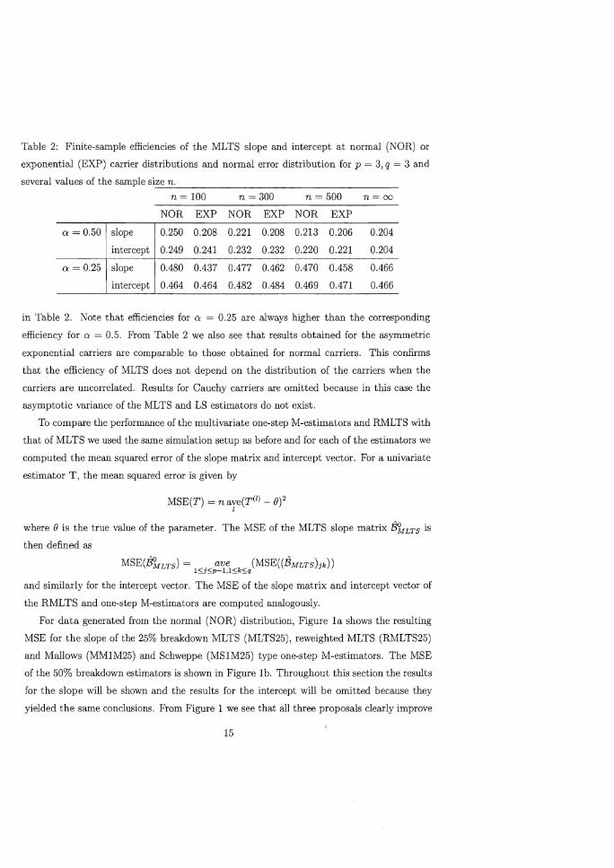
Table 2: Finite-sample efficiencies of the MLTS slope and intercept at normal (NOR) or

exponential (EXP) carrier distributions and normal error distribution for p = 3, q = 3 and

several values of the sample size n.

n = 100 n = 300 n = 500 n= 00

NOR EXP NOR EXP NOR EXP

a = 0.50 slope 0.250 0.208 0.221 0.208 0.213 0.206 0.204

intercept 0.249 0.241 0.232 0.232 0.220 0.221 0.204

a = 0.25 slope 0.480 0.437 0.477 0.462 0.470 0.458 0.466

intercept 0.464 0.464 0.482 0.484 0.469 0.471 0.466

in Table 2. Note that efficiencies for a = 0.25 are always higher than the corresponding

efficiency for a = 0.5. From Table 2 we also see that results obtained for the asymmetric

exponential carriers are comparable to those obtained for normal carriers. This confirms

that the efficiency of MLTS does not depend on the distribution of the carriers when the

carriers are uncorrelated. Results for Cauchy carriers are omitted because in this case the

asymptotic variance of the MLTS and LS estimators do not exist.

To compare the performance of the multivariate one-step M-estimators and RMLTS with

that of MLTS we used the same simulation setup as before and for each of the estimators we

computed the mean squared error of the slope matrix and intercept vector. For a univariate

estimator T, the mean squared error is given by

MSE(T) = n ave(T(l) - IW I

where e is the true value of the parameter. The MSE of the MLTS slope matrix BfJ..,fLTs is

then defined as

and similarly for the intercept vector. The MSE of the slope matrix and intercept vector of

the RMLTS and one-step M-estimators are computed analogously.

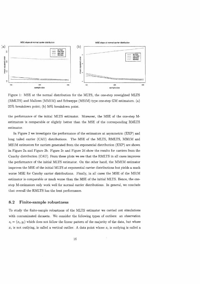
For data generated from the normal (NOR) distribution, Figure 1a shows the resulting

MSE for the slope of the 25% breakdown MLTS (MLTS25), reweighted MLTS (RMLTS25)

and Mallows (MM1M25) and Schweppe (MS1M25) type one-step M-estimators. The MSE

of the 50% breakdown estimators is shown in Figure lb. Throughout this section the results

for the slope will be shown and the results for the intercept will be omitted because they

yielded the same conclusions. From Figure 1 we see that all three proposals clearly improve

15

~a)

MSE slope at normal carrier distribution MSE slope at normal carrier distribution

(b)

--------"=--======_=_6

sample size sample size

Figure 1: MSE at the normal distribution for the MLTS, the one-step reweighted MLTS

(RMLTS) and Mallows (MMIM) and Schweppe (MSIM) type one-step GM estimators. (a)

25% breakdown point; (b) 50% breakdown point.

the performance of the initial MLTS estimator. Moreover, the MSE of the one-step M­

estimators is comparable or slightly better than the MSE of the corresponding RMLTS

estimator.

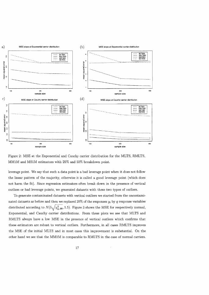
In Figure 2 we investigate the performance of the estimators at asymmetric (EXP) and

long tailed carrier (CAU) distributions. The MSE of the MLTS, RMLTS, MM1M and

MSIM estimators for carriers generated from the exponential distribution (EXP) are shown

in Figure 2a and Figure 2b. Figure 2c and Figure 2d show the results for carriers from the

Cauchy distribution (CAU). From these plots we see that the RMLTS in all cases improves

the performance of the initial MLTS estimator. On the other hand, the MM1M estimator

improves the MSE of the initial MLTS at exponential carrier distributions but yields a much

worse MSE for Cauchy carrier distributions. Finally, in all cases the MSE of the MSIM

estimator is comparable or much worse than the MSE of the initial MLTS. Hence, the one­

step M-estimators only work well for normal carrier distributions. In general, we conclude

that overall the RMLTS has the best performance.

8.2 Finite-sample robustness

To study the finite-sample robustness of the MLTS estimator we carried out simulations

with contaminated datasets. We consider the following types of outliers: an observation

Zi = (Xi, Yi) which does not follow the linear pattern of the majority of the data, but whose

Xi is not outlying, is called a vertical outlier. A data point whose Xi is outlying is called a

16

a)

c)

MSE slope at Exponential carrier distribution

------------------

. -----------., ------

sample size

MSE slope at Cauchy carrier distribution

sample size

(b)

(d)

MSE slope at Exponential carrier distribution

300

sample size

MSE slope at Cauchy carrier distribution

-----------------.O-------------_______ .a

·--· .. ···-.·· __ ··· .. ···•···•· .. ··•··········· •.• 0 .. ....•............•..........•................ c

sample size

Figure 2: MSE at the Exponential and Cauchy carrier distribution for the MLTS, RMLTS,

MMIM and MSIM estimators with 25% and 50% breakdown point.

leverage point. We say that such a data point is a bad leverage point when it does not follow

the linear pattern of the majority, otherwise it is called a good leverage point (which does

not harm the fit). Since regression estimators often break down in the presence of vertical

outliers or bad leverage points, we generated datasets with these two types of outliers.

To generate contaminated datasets with vertical outliers we started from the uncontami­

nated datasets as before and then we replaced 20% of the responses Yi by q response variables

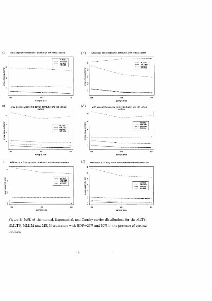
distributed according to N(5Jx~,.99' 1.5). Figure 3 shows the MSE for respectively normal,

Exponential, and Cauchy carrier distributions. From these plots we see that MLTS and

RMLTS always have a low MSE in the presence of vertical outliers which confirms that

these estimators are robust to vertical outliers. Furthermore, in all cases RMLTS improves

the MSE of the initial MLTS and in most cases this improvement is substantial. On the

other hand we see that the MMIM is comparable to RMLTS in the case of normal carriers.

17

It still improves the MSE of the initial MLTS in the case of exponential carriers and 50%

breakdown point, but in the other situations it is worse than the initial MLTS. Finally, the

MS1M in almost all cases gives a much worse result than the initial MLTS which shows

that the gain in efficiency obtained by MSIM leads to an increased bias in the presence of

outliers.

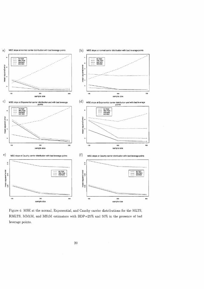
To generate contaminated datasets with bad leverage points we started from the uncon­

taminated datasets as before and then we replaced 20% of the data with observations for

which the p - 1 independent variables were generated according to N(5JX~-I .. 99' 1.5) and

the q dependent variables were generated from N(5.JX~ .. 99' 1.5). Figure 4 shows the MSE

for respectively normal, Exponential, and Cauchy carrier distributions. From these plots we

see that MLTS and RMLTS always have a low MSE in the presence of bad leverage points,

hence these estimators are also robust to bad leverage points. As before, we also have that

in all cases RMLTS improves the MSE of the initial MLTS. On the other hand, the MMIM

improves the MSE of the initial MLTS in case of normal or exponential carriers, and can even

be better than RMLTS, but it is much worse for the Cauchy carrier distribution. Finally,

as with vertical outliers, in most cases the MSE of MS1M is much worse than the MSE of

the initial MLTS. Note that for Cauchy carrier distributions we have omitted the MSE of

MSIM because it was even much bigger than the MSE of the initial MLTS.

To summarize, our simulations with contaminated datasets confirmed that vertical out­

liers and bad leverage points have a small influence on the MLTS and RMLTS estimators,

thus MLTS and RMLTS are robust to vertical outliers as well as bad leverage points. In all

cases the RMLTS improved the result of the initial MLTS. On the other hand we noted that

outliers can have a much higher influence on the one-step M-estimators which can perform

much worse than the initial MLTS in the presence of outliers.

9 Example

To illustrate the MLTS method in practice, we use a real dataset of Charnes et al. (1981).

This dataset consists of 70 observations on 5 explicative variables and 3 response variables.

For students of 70 school sites in the U.S. the following five inputs were measured: education

level of mother (Xl), highest occupation of a family member (X2), number of parental visits

to the school (X3), parent counseling concerning school-related topics (X4), and the number

of teachers at the school site (xs). The three outputs are the total reading score measured

18

a)

c)

~ )

MSE slope at normal carrier distribution with vertical outliers

sample size

MSE slope at Exponential carrier distribution and with vertical outliers

sample size

MSE slope at Cauchy carrier distribution and with vertical outliers

1-.------ MLTS25 1 - AMLTS25 --- MM1M25 ~ ... -.". MS1 M25

sample size

(b)

(d)

(f)

MSE slope at normal carrier distribution with vertical outliers

'====,--------------------,

sample size

MSE slope at Exponential carrier distribution and with vertical outliers

--------- -- 0--__________________ _

sample size

MSE slope at Cauchy carrier distribution and with vertical outliers

--------------------u--__________________ ~

.............. -............ -----......... -....... g ................................................. e

sample size

Figure 3: MSE at the normal, Exponential, and Cauchy carrier distributions for the MLTS,

RMLTS, MM1M and MS1M estimators with BDP=25% and 50% in the presence of vertical

outliers_

19

a)

c)

e)

MSE slope at normal carrier distribution with bad leverage points

~, ........... . 100 300

sample size

MSE slope at Exponential carrier distribution and with bad leverage points

'00 '" sample size

MSE slope at Cauchy carrier distribution with bad leverage points

'"

d ---------------_________ , _____________________ "

I······· MLTS" 1 - RML.TS25 --- MM1M25

. -~-. 5"

sample size

(b) MSE slope at normal carrier distribution with bad leverage pOints

,00 500

sample sIze

(d) MSE slope at Exponential carrier distribution and with bad leverage

6 ~.

" I m .. -E

(f)

points

a,:.:_~:~~,

'" "~""",,_ ·-n··························· .. ·······

~,,--------------------" " ,

"'" sample size

MSE slope at cauchy carrier distribution with bad leverage points

0----------___________ 0 ____________________ "

I······· MLTS2' 1 - RMLTS25 --- MM1M2S

g~g ......................... . ·········ii

"'" sample size

Figure 4: MSE at the normal, Exponential, and Cauchy carrier distributions for the MLTS,

RMLTS, MMIM, and MSIM estimators with BDP=25% and 50% in the presence of bad

leverage points.

20

Table 3: Estimates of the regression parameters for the school data obtained by RMLTS

with 25% BPD and trimming proportion 5 = 0.01 and by least squares. the last column are

the intercept estimates.

RMLTS-estimator

0.098 4.760 0.087 -0.750 -0.171 1.998

0.031 5.146 0.115 -0.713 -0.228 2.616

-0.013 1.575 0.270 0.003 0.035 0.176

LS-estimator

0.203 3.745 -0.283 -0.091 -0.181 -0.179

0.110 4.770 -0.529 0.143 -0.341 -0.366

-0.045 2.227 0.195 -0.056 0.011 -0.041

by the Metropolitan Achievement Test (Yl), the total mathematics score measured by the

Metropolitan Achievement Test (Y2), and the Coopersmith self-esteem inventory (Y3). We

consider a multivariate regression model with intercept, hence p = 6 and q = 3. We applied

the one-step reweighted MLTS regression with a = 0.25 and 5 = 0.99 to these school data

and we denote the resulting fit as BRMLTS. The estimate for the covariance of the errors

is denoted as t RMLTS. The estimates of the regression coefficients are reported in Table 3

together with the classical least squares estimates. We see that there are differences both

in magnitude and sign between the RMLTS and LS estimates indicating the presence of

outliers that influenced the classical estimates.

In order to detect outliers in multivariate linear regression we construct the following

diagnostic plot. First we compute the robust distances di(BRMLTS, tRMLTS) in the q­

dimensional residual space. Then we compute the one-step reweighted MCD mean T~_l (X)

and scatter C~_l (X) of the explanatory variables and obtain the corresponding robust dis­

tances h(Xi) in the space of explicative variables. Since, for outlier-free samples, h(Xi)2 and

d;(BRMLTS, tRMLTS) roughly have chi-squared distributions with p - 1 and q d.f., respec­

tively, we can classify the ith observation as a high leverage point if h(Xi)2 > X~,p-l' and

as a multivariate regression outlier if d~(BRMLTS' t RMLTS) > X~,q where X~,r denotes the

5 quantile of a Chi-square distribution with r d.f. Plotting the robust residual distances

di(BRMLTS, tRMLTS) versus the robust distances h(Xi) of the Xi and drawing the cutoff lines

h = J X~'P-l and d = ~ allows us to detect vertical outliers, good and bad leverage

points. This plot is a generalization to multivariate regression of the diagnostic plot pro-

21

Diagnostic plot based on RML TS

-59

_1221 -35

-44

_24-18 -20 -33 -52

- -54

--' .. -- --: ........... -68 -S7e46 -67 , -& •••• \ • 1 .. 66 -50 -3 -10

2 6 10 12

Robust distance of X

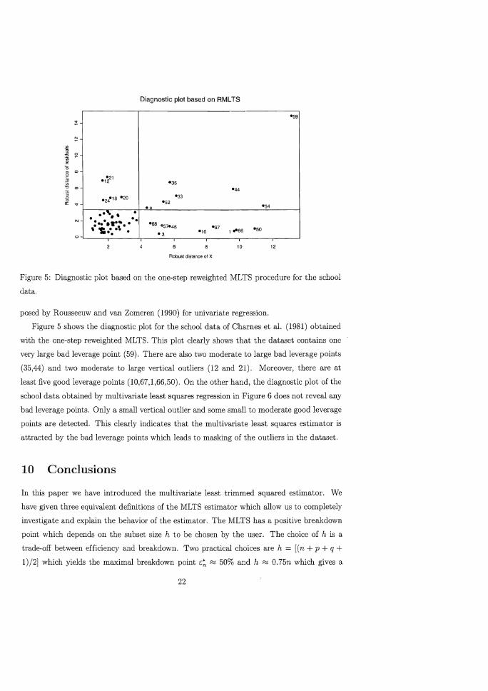
Figure 5: Diagnostic plot based on the one-step reweighted MLTS procedure for the school

data.

posed by Rousseeuw and van Zomeren (1990) for univariate regression.

Figure 5 shows the diagnostic plot for the school data of Charnes et al. (1981) obtained

with the one-step reweighted MLTS. This plot clearly shows that the dataset contains one

very large bad leverage point (59). There are also two moderate to large bad leverage points

(35,44) and two moderate to large vertical outliers (12 and 21). Moreover, there are at

least five good leverage points (10,67,1,66,50). On the other hand, the diagnostic plot of the

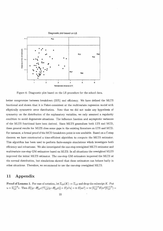
school data obtained by multivariate least squares regression in Figure 6 does not reveal any

bad leverage points. Only a small vertical outlier and some small to moderate good leverage

points are detected. This clearly indicates that the multivariate least squares estimator is

attracted by the bad leverage points which leads to masking of the outliers in the dataset.

10 Conclusions

In this paper we have introduced the multivariate least trimmed squared estimator. We

have given three equivalent definitions of the MLTS estimator which allow us to completely

investigate and explain the behavior of the estimator. The MLTS has a positive breakdown

point which depends on the subset size h to be chosen by the user. The choice of h is a

trade-off between efficiency and breakdown. Two practical choices are h = [(n + p + q + 1)/2] which yields the maximal breakdown point c~ "" 50% and h "" 0.75n which gives a

22

Diagnostic plot based on LS

"35

" " " " " "

" "" "33 "59

" " "44

" "" " " " " " ""

\. , " " " "" "

" " " " " : " " " "" " " ": " "67

" "66 ... ., "

" 4

Mahalanobis distance of X

Figure 6: Diagnostic plot based on the LS procedure for the school data.

better compromise between breakdown (25%) and efficiency. We have defined the MLTS

functional and shown that it is Fisher-consistent at the multivariate regression model with

elliptically symmetric error distribution. Note that we did not make any hypothesis of

symmetry on the distribution of the explanatory variables, we only assumed a regularity

condition to avoid degenerate situations. The influence function and asymptotic variances

of the MLTS functional have been derived. Since MLTS generalizes both LTS and MCD,

these general results for MLTS close some gaps in the existing literature on LTS and MCD.

For instance, a formal proof of the MCD breakdown point is now available. Based on a C-step

theorem we have constructed a time-efficient algorithm to compute the MLTS estimator.

This algorithm has been used to perform finite-sample simulations which investigate both

efficiency and robustness. We also investigated the one-step reweighted MLTS estimator and

multivariate one-step GM estimators based on MLTS. In all situations the reweighted MLTS

improved the initial MLTS estimator. The one-step GM estimators improved the MLTS at

the normal distribution, but simulations showed that these estimators can behave badly in

other situations. Therefore, we recommend to use the one-step reweighted MLTS.

11 Appendix

Proof of Lemma 1. For ease of notation, let ~Ls(K) := ~LS and drop the subscript K. Put

u = ~Llj2E:. Then E[(y-Bisx)t~L1(y-Bisx)] = E[utu] = tr E[uut] = tr (~L~/2 E[E:E:t]~L~/2) =

23

tr Iq = q, SO (BLS , I: LS ) satisfies condition (2.4). Take any bE mpxq and any b. a positive

definite symmetric matrix of size q such that (2.4) holds. There exists an orthogonal matrix

P and Al 2: .. , 2: Aq > 0 such that 6. = I:~;PAPtI:~; where A = diag(AI, ... ,Aq). Put

v = ptI:~~/2 (y - btx). Then we obtain

q

q = E[(y - bt4f:>. -I(y - btx)] = E[vtA -Iv] = L A;-I E[v?] i=l

On the other hand, since E[xct ] = 0, we have that

ptI:~~/2E[(E + (BLS - b)tX)(E + (BLS - W4]I:~~j2 P

pt(Iq + l'..~~/2(BLS - b)tE[xxt] (BLS - b)l'..~y2)p

Iq + ((BLS - b)l'..~~/2 P)tE[xxt] ((BLS - b)I:~y2 Pl.

Taking the diagonal elements of (11.2) and inserting them in (11.1) yields

q q q

(11.1)

(11.2)

q = L .\;-1 + L .\;-1 ((BLS - b)l'..~~/2 P);E[xxt]((BLS - b)I:~~/2 P)i 2: LA;-I, (11.3) i=l i=l i=l

with ((BLS - b)I:~y2p)i the i-th column of this matrix. Furthermore, by definition of b.

and the relation between an arithmetic and geometric mean, we have

(11.4)

From the last two inequalities (11.3) and (11.4) we see that detI:Ls ::::: detb., showing

already that (BLS , I: LS ) solves the minimization problem.

Moreover, equality in (11.3) only occurs if all ((BLS - b)I:~~/2 P)i = 0, thus if b = BLS . In

order to have det I: LS = det b., also (11.4) needs to become an equality, which can only occur

if all Ai are equal to one, implying b. = I:LS . Hereby, we have also proved the uniqueness

part. o

Proof of Proposition 1: Take H E argmin det tLs(H). We first prove that BLS(H) H

minimizes det MCDq(B). Take B E IRpxq arbitrarily, then by definition of the MCD there

exists a HE H such that MCDq(B) = Covo(H, B). Using properties of traces, it follows that

1 h L Tj(B)(Covo(H,B))-ITj(B)t = q. jEH

(11.5)

Since the data are in general position, Lemma 1 can be applied:

24

where we applied the definition of Hand MCDq. We conclude that BLs(H) E argmin det MCDq(B). B

On the other hand, take now 13 E argmindetMCDq(8) By definition of MCD, there B

exists a H E 1{ such that MCDq(B) = Cova(H,8) and in particular det CovaCH, B) ~

det CovaCH, BLs(H)). But since (11.5) also holds for the pair (H, 8), the uniqueness part of

Lemma 1 gives 8 = BLs(H). It then follows that for any other H E 1{ we have

Hence, we have that H E argmin det I:-Ls(H) which ends the proof. o H

Proof of Proposition 2: For any HE 1{ denote tLs(H) := (dettLs(H))-l/qtLS(H) such

that det tLs(H) = 1. We first give the following equations which will be useful to prove the

result. Using properties of traces, we find that

We also have that

1 "'- 1 - - t "htr L..J I:-Ls(H)- rj(BLs(H)h(BLS(H)) jEH

trtLs(H)-1tLS(H) = q. (11.6)

L d;(BLS(H), tLs(H)) = (det t Ls(H))-1/q L d;(BLS(H), tLs(H)) (11.7) jEH jEH

Combining (11.7) with (11.6) yields

L d;(BLS(H), tLS(H)) = hqdet t Ls(H))1/q. jEH

(11.8)

We first prove that for any H E argmin det tLs(H) we have that BLs(H) E {8 1(13, t) E H

h - -argmin 2:j =1 dJ,n(B, I:-)}. Take H E argmin det I:-Ls(H) and denote B,E;IEI=1 H

the set of indices corresponding to the first h ordered squared distances of the residuals.

Now suppose that

h

L dJ,n(BLS(H), tLs(H)) = L d;(BLS(H), tLs(H)) < L d;(BLS(H), tLS(il)). j=1 JEW jEff

Using (11.7) and (11.8), this yields * 2: jEHI dJ(BLs(H), tLs(H)) < q. Therefore, there

exists a constant 0 < c < 1 such that * 2:jEHI d;(BLs(H), ctLs(H)) = q. It then follows

25

from Lemma 1 that det tLs(H') < det ctLs(H) < det tLs(H) which is a contradiction, so

we conclude that h

L dJ,n (13Ls (iI), f'.LS(iI)) = L d] (BLS (iI), f'.Ls(H)). (11.9) j=l

Now suppose that there exists some B E IRpxq and L; E PDS(q) with det L; = 1 such that

h h

LdJ,n(B,2:) < LdJ,n(BLS(iI),f'.LS(H)) (11.10) j=l j=l

Denote HI := {jl dj(B, L;) :S dh:n(B, L;)} E 7i the set of indices corresponding to the first h

ordered squared distances of the residuals and suppose that

h ~2 ~2 ~2~ -L..- dj:n(B, 2:) = L..- dj(B, 2:) < L..- dj(BLS(H1), 2:Ls(H1)).

j=l jEH, jEH,

Using (11.8) this implies that ~ ~jEHl d;(B, det tLs(H1)ljqL;) < q. Hence, there exists a

constant 0 < c < 1 such that ~ ~jEHl d](B, cdet tLs(H1)ljqL;) = q. From Lemma 1 it follows

that det tLs(Hd < det (cdet tLs(H1)ljqL;) = cq det tLs(Hd which is a contradiction, so we

have that h

L d].n(B, 2:) 2: L d](BLS(Hd, f;LS(H1)). j=l jEH,

From (11.9) and (11.11) it follows that the inequality (11.10) implies that

L d](BLs(HIl, f'.Ls(H1)) < L d](BLS(iI), tLs(iI)). jEH,

(11.11)

(11.12)

But, using (11.8), this can be rewritten as hq det tLs(H1)ljq < hq det tLs(H)ljq. Hence, we

obtain det tLs(Hd < det tLs(H) which is a contradiction since H E argmin det tLs(H). H

Therefore, we conclude that

h h

LdJ,n(BLS(H),f'.LS(iI)):s Ld],n(B,L;) j=l j=l

for all B E IRpxq and L; E PDS(q) with det L; = 1 and thus we have ihs(H) E {8 1(8, t) E

argmin ~~=1 dJ,n(B, L;)}. B,E;IEI=l

- - h -We now prove that for any (B, L;) E argmin ~j=l d}n(B, L;) there exists a H E 7i such

B,E;IEI=l

that 8 = 8Ls(H) and H E argmin det tLs(H). Denote H := {jl dj(8, t) :S dh:n(8, t)} E 7i H

the set of indices corresponding to the first h ordered squared distances of the residuals, then

we have that h

L d].n(B, f;) = L d](B, f;) :S L d](BLS(iI), f;LS(H)). (11.13) j=l

26

Using (11.8) it follows that * L;jEH d;(B, det ELS(H)I/q E) ::; q. Hence, there exists a

constant 0 < c::; 1 such that * L;jEH d;(B, cdet ELS(H)I/q E) = q. From Lemma 1 we then

obtain that det ELS(H) ::; det (cdet ELS(H)I/q E) = cq det ELS(H) which is a contradiction

unless if c = 1 and by Lemma 1 (uniqueness) we then have that B = BLS(H) and E = ELS(H). For any H E 7-i we now have that

h

L 4n(13, t) = L d;(BLS(H), tLs(H)) ::; L d;(BLS(H), tLs(H)) j=1 jEH

By using (U.8) the inequality can be rewritten as hq det ELS(H)I/q ::; hq det ELS(H)I/q

which yields det ELS(H) ::; det ELS(H) for all H E 7-i. Therefore, we conclude that H E

argmin det ELS(H) which ends the proof. o H

Proof of Theorem 1: We first prove that f~(BMLTS, Zn) 2': min(n - h + 1, h - k(Zn))jn.

We will show that there exists a value M, which only depends on Zn, such that for every

Z~ obtained by replacing at most m = min(n - h + 1, h - k(Zn)) - 1 observations from Zn

we have that IIBMLTS(Z~)II ::; M. The matrix norm we use here is IIAII = sup IIAull where lIull=1

u E IR5 and A E IRpxq. Sometimes we will also use the L2-norm IIAI12 = (L;i,j laij 12)1/2. Since all norms on IRpxq are topologically equivalent there exist values 0:1,0:2 > 0 such that

O:lllAl1 ::; IIAlh::; 0:211AII for all A E IRpx q.

Let J be a subset of size k(Zn) + 1. Then there cannot be a hyperplane such that all Xj

with j E J are on it. Therefore

where "/ E IRP. Furthermore it is excluded that there exists a 8 E IRp+q such that Yj - 8 txj

for all j E J are lying on a (q - 1) dimensional hyperplane. Indeed, otherwise there exists

an 0: E IR5 such that for all j E J we have ol(Yj - 8 txj) = o:tyj - "/tXj = 0 where "/ = 80:. However, this contradicts the assumption #J = k(Zn) + 1. Since for all 8 E IRp+q the

Tj := Yj - stXj are not lying on a (q - 1) dimensional hyperplane, we have that

where Covo( {Tj; j E J}) = k(Z~)+l L;jEJ TjT} and Amin denotes the smallest eigenvalue of that

matrix. Denote

c = min (min(cl (J), C2(J))) > 0 J

27

(11.14)

where the minimum is over all subsets J of size k(Zn) + 1 and define

M = supI18LS(H)tll < 00 HE'H

(11.15)

since no h points of {Xi; i = 1, ... , n} are lying on the same hyperplane (k( Zn) < h). Let

Ny = max IIYil1 and Nx = max Ilxill. Put V = (Ny + M Nx )2q and l:S~.'Sn 1$1:Sn

(11.16)

Now take a dataset Z~ obtained by replacing m observations from Zn and suppose IIBMLTS(Z~) II > M. First of all, there exists a subset HI E 1t containing indices only corresponding to

data points of the original dataset Zn. Using lemma 5.1 of Lopuhaii. and Rousseeuw (1991,

page 244) and properties of norms it follows that

det(I:Ls(HI)) ::; Amdcov({rj(BLs(HI));j E HI})q 1"" A A t ::; (J; 6 Amax(rj(BLS(HI))rj(BLS(HI)) ))q

jEH,

1"" A 2 (J; 6 Ilrj(BLs(HI))11 )q jEH,

1"" A t 2 ::; (J; 6 (11Yjll + IIBLS(HI) xjll) )q jEH,

::; (Ny + M Nx )2q

V (11.17)

where Amax denotes the largest eigenvalue of a matrix. Now let H2 be the optimal subset

corresponding to BMLTS(Z~) such that BMLTS(Z~) = BLS(H2) := 8 2 . Since h-m ~ k(Zn)+

1 the set H2 contains a subset J of size k(Zn) + 1 corresponding to original observations of

Zn. Using lemma 5.1 of Lopuhaii. and Rousseeuw (1991, page 244) we obtain

(11.18)

On the other hand,

(11.19)

28

By definition of Cl (J) there exists at least one index ]0 E J C H2 such that

j=l

(11B2112 q(J))2

2': (QIIIB21Iq(J))2

which yields 118~xjoll > O'lAlc. Since by definition QIMc 2': Ny we obtain IIYjo - 8~xjoll 2': IIIYjoll-118~xjolll > O'lMc - Ny. By taking u = to=~~XjOII it follows from (11.19) that

YJO 2XJO

Amax(tLs(H2)) 2': IIYjo - B~xjol12 /h > (QIMc - Ny)2/h. (11.20)

Combining (11.20) and (11.18) yields

, 1 - 2 k( Zn) + 1 1 det(ELs(H2)) > y;(Q1Mc - Ny) ( h c)q- = V

by definition of M. Together with (11.17) this implies det(f:Ls(H2)) > det(tLs(H1)) which

contradicts the definition of BMLTS(Z~), so we conclude that IIBJVILTS(Z~)II ::; M. We now prove that also E:~(BMLTS, Zn) ::; min(n - h + 1, h - k(Zn))jn. First we show

that E:~(BMLTS' Zn) ::; (n - h + l)jn. Indeed, if we replace n - h + 1 points of Zn then the

optimal subset H2 of Z~ will contain at least one outlier and we know that least squares

can explode in the presence of even a single outlier. It then follows that also BMLTS(Z~)

explodes.

Now we show that E:~(BMLTS,Zn) ::; (h - k(Zn))jn. Denote j C {I, ... ,n} the set of

indices corresponding to the k(Zn) observations from Zn lying on a hyperplane of IRp+q.

Then there exist a 0' E IRq and, E IRP such that ciYj - ,tXj = 0 for all j E 1. If 0' of 0 then there exists a 8 E IRp+q such that BO' = , which implies O't(Yj - 8 txj) = 0

for j E 1. Therefore, for j E J we have that Yj - Btxj E S where S is a (q - 1) dimensional

subspace of IRq. Now take a D E IRpxq with IIDII = 1 such that {Dtx; x E IRP} c S. Now

replace m = h - k(Zn) observations of Zn, not lying on S, by (xo, (8 + AD)txo) for some

arbitrarily chosen Xo E IRP and A E IR. Denote Jo the set of indices corresponding to the

outliers. It follows that for the m outliers Tj(8 + AD) = 0 and for the k(Zn) points on S we

have that Tj(B + AD) = Yj - 8 txj - ADtxj E S. Therefore {Tj(8 + AD);] E J U Jo } belongs

to the subspace S, giving a zero determinant for the matrix covo( {Tj(B + XD); j E J U Jo })

Therefore, using Proposition 1 it follows that BMLTS(Z~) = 8 + AD which tends to infinity

when A -> 00.

29

If a = ° then we have that "'/Xj = 0 for all j E 1. Now replace m = h - k(Zn) other

observations of Zn by observations on the hyperplane "/x = 0. Denote H2 the set of indices

corresponding with observations of Z~ such that "-/x = 0. Since all these observations

belong to a hyperplane of IRp+q we have that det cov({Yj - HLS(H2)tXj;j E H2 }) = 0.

But since 'ylx = 0 is a vertical hyperplane we have IIHLs(H2) II IIHMLTs(Z~)11 = 00.

00 and it follows that

o

Proof of Corollary 1. Since for q = 1 we have det(tLs(H2)) = AmaxCtLS(H2)), we do not

need to establish the lower bound (11.18) and thus we do not need C2(J) > o. To obtain

C1(J) > 0 it suffices to consider datasets of size k'(Zn) + 1. Therefore, the result immediately

follows from the previous proof if we replace k(Zn) by k'(Zn). 0

Proof of Theorem 2. Using properties of traces we obtain

(11.21)

and similarly -k '2: iEHl d;(Hl , t l ) = q. By definition of H2 we have

(11.22)

and also c > 0 since det(t2) > O. Combining (11.21) and (11.22) yields

1", 't' 1,1",2" cq h L. rj(BIl (cEIl- rj(B1) = ch L. dj (B1 , E1) = ~ = q. jEH, jEH2

(11.23)

From Lemma 1 it follows that det(t2) ~ det(ctJ) and (11.22) implies det(ctJ) ~ det(t1),

hence det(t2) ~ det(t1). Moreover, from Lemma 1 we know that det(t2) = det(ct1) iff

H2 = Hl and t2 = ct1 . Furthermore, det(ctd = det(td iff c = 1. Therefore, det(t2) = det(td iff H2 = HI and t2 = t 1 . 0

Proof of Lemma 2. Clearly, we have that E E DH(a). Note that

_1_ j d2(x, y) dH = _l_tr j d2(x,y) dH = tr (EA(H)-lEA(H)) = trIq = q I-a A I-a A

30

On the other hand, we have that

( ,d2(x, y) dH + ( ,d2(x, y) dH lenA le\A

:S (, d2 (x, y) dH + D~PH(£ \ A) lenA

( ,d2(x, y) dH + D~PH(A \ £) lenA

:S ( ,d2(x, y) dH + f, d2 (x, y) dH lenA 1.4v L d2 (x,y)dH

Therefore, there exists a 0 < c ::; 1 such that

(11.24)

Since A is an MCD solution, we have that det (c L, AJ H)) ::; det L, AJ H) ::; det L,e (H) which

in combination with (11.24) contradicts lemma 1 unless if B;..(H) = Bc(H) and CL,;..(H) =

L,e(H). Then c should also be equal to 1. 0

Proof of Theorem 3. First of all, due to equivariance, we may assume that B = 0 and

L, = Iq, so y = c ~ F. It now suffices to show that BLTS(H) = O. Then we will have that

L,LTS(H) is the MCD functional at the distribution of y - BLTS(H)tx = Y = c. Since the

factor c" makes the MCD Fisher-consistent at elliptical distributions (see Butler et al. 1993,

Croux and Haesbroeck 1999) it will follow that L,LTS(H) = Iq. Lemma 2 shows that BLTS is

the least squares fit based solely on the cylinder C = {(x, y) E IRp+q; (y - BirSX)tL,L~S(Y­

Birsx) ::; D~}. Therefore,

(11.25)

Now suppose that BLTS =f O. Let A1, ... , Aq be the eigenvalues of L,LTS and V1," ., Vq the

corresponding eigenvectors. There will be at least one 1 ::; j :::; q such that BLTSVj =f O.

(Note that BLTS is not necessarily of full rank.) Fix this j. From (11.25) it follows that we

should have 1 v}(Birsx)(y - Birsx)tVj dF(y) dG(x) = 0

which can be rewritten as

with

( V} (Birsx)J(x) dG(x) = 0 lIRP

31

(11.26)

where Cx = {y E mql(x, y) E C}. Fix x and set d = (d1 , ... , dq)t := Birsx. Since y

is spherically symmetrically distributed, for computing lex) we may assume w.l.o.g. that

L,LTS = diag(Al, ... , Aq) as well as Vj = (1,0, ... ,0). For every d1 - ~ :::: Yl :::: d1 + ~ denote

C(Yl) = {(Y2"" ,Yq) E iRq-II t (Yj ~dj)2 ::; c _ (Yl ~ dd} j=2 J 1

where c := D;, > O. Then we can rewrite lex) as

Since C(d1 + t) = C(d1 - t) it follows that

If d1 > 0 we have (d1 + t)2 + y~ + ... + Y~ > (d1 - t)2 + y~ + ... + Y~ (for t > 0) and since

9 is strictly decreasing this implies lex) < O. Similarly, we can show that d1 < 0 implies

l(x) > 0 and that d1 = 0 yields lex) = O. Hence, we have shown that vj(Birsx) > 0 implies

lex) < 0 and if vj(Birsx) = 0, then lex) > O. Also, vj(B)irsx) = 0 implies lex) = O.

However, due to condition (5.6), the latter event occurs with probability less than 1 - a.

Therefore, we obtain fIRP vjBirsx lex) dG(x) < 0 which contradicts (11.26), so we conclude

that BLTS = O. 0

Proof of Theorem 4. Consider the contaminated distribution H. = (1- c)Ho +cL~,zo with

Zo = (xo, Yo) and denote B. := BLTS(R) and 2:. := L,LTs(H,J Then (5.3) results in

B. = (hE XXtdH.(x,y») -1 h, xytdH.(x,y)

where A. E VH,(a) is an MLTS solution. Differentiating w.r.t. c and evaluating at 0 yields

IF(zo; BLTS, Ho) = (h xxt dHo(z») -1 :0 h, xyt dH,(z)I,=o + :0 [ (h, xxt dH.(Z») -1] 1.=0 h xyt dHo(z)

Lemma 2 combined with Fisher-consistency yields that A = {(x, y) E m p+q ; yty :::: qaJ where qa. = (D})-I(l - a) with D}(t) = Pp(IIYI12 :::: t). Hence A = m p x {y E m q; liyl12 :::: qa.} =: mp x A. This implies

f,xytdHo(z) = f xdG(x) f ytdF(y)=O 1A JIRP JA

32

by symmetry of F and

j . xxt dHo(z) = ( xxt dG(x) j dF(y) = EG[xxt] (1 - a) A JIRP A

Therefore, we obtain

IF(zo; BLTS, Ho)

Similarly to Proposition 1 of Croux and Haesbroeck (1999), it can be shown that Lemma 2

still holds for contaminated distributions HE' Let us denote d;(x, y) = (y-B~x)tL;;I(y-B;x), then it follows that A£ = {(x, y) E IRp+q; d;(x, y) ::; q,,(f)} where q,,(f) = (D1J-l(1-a) with

Dk,(t) = PH,(d;(x,y) ::; t). For x fixed we define the ellipsoid [e,x := {y E IRq; d;(x, y) ::;

qa(f)}. Then it follows that

j. xyt dHo(z) = 11 xyt dF(y)dG(x) = r x (r y g(yty) dY) t dG(x). A£ JRF Ee,x JIRF J£e:;,x

(11.28)

Using the transformation v = L;;1/2(y - B;x), we obtain that

1(10) := 1 y g(yty) dy = det(l;£)1/2 r (l;!/2v + B~x)g((l;!/2v + B~x)t(l;!/2v + B;x)) dv. C'.X JllvIl 2 :Sqa(e)

Rewriting this expression in polar coordinates v = re({}) where r E [0, Vq,,(c)], e({}) E Sq-l

and {} = ({}l, ... , (}q-Il E e = [0, 7r[ X ... x [0, 7r[ X [0, 27r[, yields

where J( {}, r) is the Jacobian of the transformation into polar coordinates. Applying Leibniz'

formula to this expression and using the symmetry of F results in

~I(c)1 = r ~ ((l;!/2v + B;x)g((l;!/2v + B~x)t(l;;/2v + B;x))) dv & e=O invll2 :Sqa & le=o

(11.29)

The derivative on the right hand side becomes

() & {(l;!/2v + B~x)g((l;!/2v + B~x)t(l;!/2v + B~x))}I£=o =

{IF(zo; l;~is, Ho)v+IF(zo; BLTS, Ho)tx }g(vtv)+2 vg'(vtv){(vt IF(zo; l;~is' Ho)v+vt IF (zo; BLTS, Ho)t x }

(11.30)

33

Since ~lvll'SqQ vg(vtv) dv and ~lvll'SqQ vg'(vtv)vt IF(zo; r;Z';'s, Ho)v dv are zero due to sym­

metry of F, the terms in (11.30) including IF(zo; r;Z';'s, Ho) give a zero contribution to the

integral in (11.29). It follows that

(1- a)IF(zo; BLTS, Ho)tx + 2 { g'(vtv)vvt dv IF(zo; BLTS, Ho)tx Jllvll'SqQ

[(1 - a) + 2C2] IF(zo; BLTS , Ho)tx

where C2 = ~lvll'SqQ g'(vtv)vr dv can be rewritten in the form given in Theorem 4 by using

polar coordinates. From (11.28) we now obtain that

(11.31)

Substituting (11.31) in (11.27) yields

which results in

o

References

Bai, Z.D., Chen, N.R., Miao, B.Q., and Rao, C.R. (1990), "Asymptotic Theory of Least

Distance Estimate in Multivariate Linear Models," Statistics, 21, 503-519.

Bilodeau, M. and Duchesne P. (2000), "Robust Estimation of the SUR Model," The Cana­

dian Journal of Statistics, 28, 277-288.

Butler, R.W., Davies, P.L., and Jhun, M. (1993), "Asymptotics for the Minimum Covariance

Determinant Estimator," The Annals of Statistics, 21, 1385-1400.

Charnes, A., Cooper, W.W., and Rhodes, E., (1981), "Evaluating Program and Managerial

Efficiency: An Application of Data Envelopment Analysis to Program Follow Through,"

Management Science, 27, 668-697.

Coakley, C.W. and Hettmansperger, T.P. (1993), "A Bounded Influence, High Breakdown,

Efficient Regression Estimator," Journal of the American Statistical Association, 88, 872-

880.

34

Croux, C., and Haesbroeck, G. (1999), "Influence Function and Efficiency of the Mininmum

Covariance Determinant Scatter Matrix Estimator," Journal of Multivariate Analysis, 71,

161-190.

Croux, C., Rousseeuw, P.J., and Hossjer, O. (1994), "Generalized S-Estimators," Journal of

the American Statistical Association, 89, 1271-1281.

Donoho, D.L., and Huber, P.J. (1983), "The Notion of Breakdown Point," in A Festschriftfor

Erich Lehmann (P.J. Bickel, K.A. Doksum and J.L. Hodges, eds.), Belmont, Wadsworth,

pp 157-184.

Grubel, R (1988), "A Minimal Characterization of the Covariance Matrix," Metrika, 35,

49-52.

Hampel, F.R, Ronchetti E.M., Rousseeuw P.J., and Stahel W.A. (1986), Robust Statistics:

The Approach Based on Influence Functions, John Wiley and Sons, New York.

Hossjer, O. (1994), "Rank-Based Estimates in the Linear Model With High Breakdown

Point," Journal of the American Statistical Association, 89, 149-158.

Johnson, N.L., and Kotz, S. (1972), Distributions in Statistics: Continuous Multivariate

Distributions, John Wiley and Sons, New York.

Koenker, R, and Portnoy, S. (1990), "M Estimation of Multivariate Regressions," Journal

of the American Statistical Association, 85, 1060-1068.

Lopuhaii., H.P. and Rousseeuw, P.J. (1991), "Breakdown Points of Affine Equivariant Esti­

mators of Multivariate Location and Covariance Matrices," The Annals of Statistics, 19,

229-248.

Marrona, RA., and Yohai, V.J. (1997), "Robust Estimation in Simultaneous Equations

Models," Journal of Statistical Planning and Inference, 57, 233-244.

Ollila, E., Hettmansperger, T.P., and Oja, H. (2002), "Estimates of Regression Coefficients

Based on Sign Covariance Matrix," to appear in Journal of the Royal Statistical Society,

Series B.

Ollila, E., Oja, H., and Koivunen, V. (2001), "Estimates of Regression Coefficients Based on

Rank Covariance Matrix," submitted.

35

Rousseeuw, P.J. (1984), "Least Median of Squares Regression," Journal of the American

Statistical Association, 79, 871-880.

Rousseeuw, P.J., and Leroy, A.M. (1987), Robust Regression and Outlier Detection, Wiley­

Interscience, New York.

Rousseeuw, P.J., Van Aelst, S., Van Driessen, K., and Agull6, J. (2000), "Robust Multivari­

ate Regression," submitted.

Rousseeuw, P.J., and Van Driessen K. (1999), "A Fast Algorithm for the Minimum Covari­

ance Determinant Estimator," Technometrics, 41, 212-223.

Rousseeuw, P.J., and van Zomeren, B.C. (1990), "Unmasking Multivariate Outliers and

Leverage Points," Journal of the American Statistical Association, 85, 633-651.

Simpson, D.G., Ruppert, D., and Carroll, R.J. (1992), "On One-Step GM Estimates and Sta­

bility of Inferences in Linear Regression," Journal of the American Statistical Association,

87, 439-450.

36